
The Centre for Australian Weather and Climate Research A partnership between CSIRO and the Bureau of Meteorology
Verification of mesoscale NWP forecasts of abrupt wind changes CAWCR Technical Report No. 008 Xinmei Huang, Yimin Ma and Graham Mills December 2008


1 Centre for Australian Weather and Climate Research, Bureau of Meteorology, Melbourne GPO Box 1289,
Melbourne Victoria 3001, Australia. 2 Bushfire Cooperative Research Centre, Australia
Verification of mesoscale NWP forecasts of abrupt wind changes
CAWCR Technical Report No. 008
Xinmei Huang, Yimin Ma and Graham Mills

Enquiries should be addressed to: Dr Graham Mills Bureau of Meteorology GPO Box 1289K, Melbourne Victoria 3001, Australia [email protected]
Phone: 61 3 9669 4582
ISSN: 1836-019X ISBN: 978-1-921424-86-1 Series: Technical report (Centre for Australian Weather and Climate Research.) ; no. 8. Also issued in print.
Copyright and Disclaimer
© 2008 CSIRO and the Bureau of Meteorology. To the extent permitted by law, all rights are reserved and no part of this publication covered by copyright may be reproduced or copied in any form or by any means except with the written permission of CSIRO and the Bureau of Meteorology.
CSIRO and the Bureau of Meteorology advise that the information contained in this publication comprises general statements based on scientific research. The reader is advised and needs to be aware that such information may be incomplete or unable to be used in any specific situation. No reliance or actions must therefore be made on that information without seeking prior expert professional, scientific and technical advice. To the extent permitted by law, CSIRO and the Bureau of Meteorology (including each of its employees and consultants) excludes all liability to any person for any consequences, including but not limited to all losses, damages, costs, expenses and any other compensation, arising directly or indirectly from using this publication (in part or in whole) and any information or material contained in it.

Contents
1 Introduction 7
2 Wind Change Identification Algorithms 8
2.1 VRFC subjective wind changes . . . . . . . . . . . . . . . . . . . . . 9
2.2 Objective identification . . . . . . . . . . . . . . . . . . . . . . . . . . 9
2.2.1 Objective wind change timing and intensity . . . . . . . . . . 9
2.2.2 Pressure cycle identifications . . . . . . . . . . . . . . . . . . . 12
2.3 Meso-LAPS05 model wind changes . . . . . . . . . . . . . . . . . . . 12
3 Data and Verification Methods 13
3.1 Data . . . . . . . . . . . . . . . . . . . . . . . . . . . . . . . . . . . . 13
3.1.1 Observations . . . . . . . . . . . . . . . . . . . . . . . . . . . 13
3.1.2 Numerical model data . . . . . . . . . . . . . . . . . . . . . . 13
3.1.3 Verification stations . . . . . . . . . . . . . . . . . . . . . . . . 14
3.2 Objective verification comparisons . . . . . . . . . . . . . . . . . . . . 14
3.2.1 Matching VRFC changes with NWP model forecast changes . 15
3.2.2 Matching forecast wind changes to observation wind changes . 16
4 Verification Results 17
4.1 Model wind changes on VRFC wind change days . . . . . . . . . . . 17
4.2 Model forecasts versus observations . . . . . . . . . . . . . . . . . . . 19
5 Case Studies 20
5.1 Case 1: single cold front passage . . . . . . . . . . . . . . . . . . . . . 21
5.2 Case 2: multiple cold front/trough passages . . . . . . . . . . . . . . 23
5.3 Case 3: transitional trough . . . . . . . . . . . . . . . . . . . . . . . . 25
5.4 Case 4: distinguishable trough and cold front passages . . . . . . . . 26
6 Concluding Remarks 27
7 References 29
3


Abstract
In bush fire events, wind changes can cause abrupt changes in fire behaviour and ac-
tivity, thus endangering fire fighters. Predicting the timing of wind changes is therefore an
important aspect of fire weather forecasts. While subjective forecasts of wind change times
have been subjectively verified for some years now, there is a need to verify mesoscale NWP
forecasts of wind changes as these forecasts provide significant guidance to operational fore-
casters. Previous studies have proposed fuzzy-logic methods to objectively determine fire
weather wind changes from observations at a single surface observation station. These
methods are comprised of algorithms that diagnose the timing and the strength of the
wind changes from time series of wind direction, speed, gust, and of surface temperature,
dewpoint and pressure.
In this report, these methods are applied to both observation and NWP model forecast
time series to provide an objective verification of forecast wind change timing based on a
five-year fire season data-set over selected stations in Victoria. It is concluded that 70%
of wind changes identified with the method from model forecast are within 2.5 hours of
independent subjective wind change estimations issued from Victoria Regional Forecasting
Centre, while 93% of the subjective wind changes fall within the objective wind change
periods. Within 87% of the objectively determined major pressure trough passages, wind
change are identified from both observations and the model forecasts.
Case studies are discussed for the wind changes identified with the method under
transitional trough/cold front situations in Victoria, demonstrating the behaviour of the
algorithms in a range of situations, and also the complexities and uncertainties of deter-
mining a single wind change time.
5

1 Introduction
Wind change prediction is a crucial component of fire weather forecast services. For a
burning bush fire, a sudden wind change can turn a long fire flank into a wide fire front,
and rapidly spread the fire over a much larger area. Most dangerously, an unexpected wind
change could cause the new wide fire front to engulf the fire fighters if they are working
at what had been the previous fire flank. Fatalities have been reported on these days, and
this has led Cheney et al. (2001) to term this the “dead man zone”.
The importance of wind change forecasts to fire managers has led to the routine issu-
ing of a “Wind Change Forecast Chart” by weather forecast offices such as the Victorian
Regional Forecast Centre (VRFC) of the Bureau of Meteorology (the Bureau) “on days
when a significant (e.g. frontal) wind change is expected and the fire danger is expected
to be very high or extreme” (Bureau of Meteorology 2006). These forecasts have been
verified at the end of the fire season for recent years at selected stations in Victoria and
the results reported by Van Zetten et al. (2001) and Morgan (2002). The method used
to determine the time at which the wind change occurs relies on the skills of experienced
meteorologists and is based on spatial and temporal consistency of meteorological obser-
vations and analyses. In the remainder of this report we will refer to this method as
subjective identification. While very effective, it is a time-consuming task.
Wind changes are caused by many meteorological processes occurring on different
temporal and spatial scales. Thus there are slow and rapid, small and large, fluctuating
and persistent wind direction changes, along with a range of speed, temperature and
humidity variations. This large range of possible change structures make the development
of objective rules to identify a unique wind change time extremely challenging, yet there
are obvious benefits in being able to perform such a task. Huang and Mills (2006, 2007)
(hereafter HM06 and HM07) developed fuzzy-logic methods to determine wind change
timings at a location from single-station time-series of meteorological observations. While
the initial, and primary, aim of this algorithm was to provide a single time of maximum
wind change to be used in verification studies, it was found useful to also develop measures
of start time and end time of a wind change period, and also various measures of the
strength of the wind change. These studies showed that for some 85 percent of the wind
change forecasts issued by the VRFC, the objective and subjective wind change timings
were within 2.5 hours, and that for more than 95 percent of these changes the VRFC wind
change timing fell within the objective wind change period (HM06). Given the differences
in the two methodologies, this was considered to be a level of performance sufficient for the
objective timings to be incorporated into the VRFC verification practice for the 2005-6
and later fire seasons (Bureau of Meteorology 2008).
When applied to time series of data for all days in the fire season, rather than just
the VRFC wind change days, HM06 showed that many more wind change events were
identified, and suggested that some means of stratification of wind change days might
prove beneficial if these algorithms were to be used operationally. In southeast Australia
7

wind changes are closely linked with cold frontal passages. Such systems and their impact
on the weather and fire weather in southeast Australia have been extensively studied
(Mills 2007; Mills 2005a, b; Mills and Morgan 2006; Physick 1988; Reeder, 1986; Garratt
et al. 1989). In Western Australia, studies have shown that the transitional trough line
of the Australian west coast trough often alters the wind direction over the region in the
summer, affecting sea breezes or causing further weather change (Watson 1984; Ma and
Lyons 2000). In addition, easterly troughs extending southwards from inland Australia
can interact with mid-latitude synoptic scale troughs to bring wind changes as pre-frontal
troughs (Hanstrum et al., 1990). These associations led HM07 to develop a fuzzy-logic
algorithm to identify phases of a synoptic pressure cycle in order to stratify the objective
wind changes identified using the methods in HM06 into those occurring within synoptic-
scale trough or ridge passages, as it was found that most of the VRFC wind changes occur
during synoptic-scale trough passages (pressure minima). The combination of the HM06
and HM07 fuzzy-logic algorithms will be referred to in the remainder of this report as
objective identification.
To date the methods of HM06 and HM07 have only been applied to observation time
series. However, mesoscale numerical weather prediction (NWP) model forecasts are an
integral component of the forecast guidance used in preparing wind change forecasts, and
thus a systematic verification of the wind change forecasts from these models is of interest
to both model developers and to forecasters. As one of a series reports, following HM06
and HM07, this report first summarises the methodologies of objective and subjective wind
change timing, and then describes how HM06 and HM07 can be applied to mesoscale NWP
model forecasts to generate forecast wind change timings. Comparisons of objective wind
change identifications from model forecasts with the VRFC subjective identifications, and
with the objective identifications from the observations are presented to provide objective
verification of the operational mesoscale NWP model forecasts of wind change times on
the VRFC wind change days. Using only the VRFC wind change forecast days is a
restrictive, yet useful validation of the model forecasts, as it is on these days that forecasters
predicted significant wind changes to occur. However, it is also of interest to validate a
wider range of forecast wind changes. Using all model forecasts for several fire seasons
various other selection or stratification methodologies are employed to provide a more
general perspective on the accuracy of the NWP model wind change forecasts. Finally, a
number of case studies are presented to illustrate characteristics of objective wind change
identifications from model and observation time series, and provide a context for the
interpretation of the verification statistics.
2 Wind Change Identification Algorithms
In this section, we briefly describe all the wind change identification methods that were
used to generate the data upon which the verifications in this report are based.
8
2.1 VRFC subjective wind changes
The genesis of this project was based on the desire to verify NWP model forecasts of wind
changes on days when the VRFC issued Wind Change Forecast Charts. These are issued
on days when a significant (e.g. frontal) wind change is expected and the fire danger
is expected to be very high or extreme (Bureau of Meteorology, 2006). An example of
such a wind change forecast chart is shown in Fig. 1. At the end of each fire season
these forecasts are verified using a combination of observation and analysis time series,
and these data are referred to in this report as subjective wind change verification times.
Details of this verification process have been given in Van Zetten et al. (2001), Morgan
(2002), and Bureau of Meteorology (2006).
The VRFC subjective wind change provides only a single wind change time (tRFC)
and it is assumed that the wind change occurs instantly. It is recognised that some wind
changes are slower than are others, and that on a given day there may be more than one
significant wind change. In this case the most significant change, which is often considered
to be the final establishment of steady southwesterly post-frontal winds, will be selected as
the wind change time (Bureau of Meteorology 2006). It is routine practice for forecasters
to add comments describing the change as being shallow or deep, abrupt or gradual, etc
(Kevin Parkyn, personal communication).
2.2 Objective identification
Objective identifications use the fuzzy-logic techniques described in detail in HM06 and
HM07. There are several components of these that are described below. Using time series
of observed wind direction and speed at a single station, measures of wind change duration
and time of maximum wind change are determined, while similar approaches using wind
direction, speed, gust, and dewpoint depression are used to quantify the “strength” of
the change. Finally, applying fuzzy-logic methods to pressure time series defines phases
of the synoptic pressure cycle which allows wind changes identified with the first set of
algorithms to be classified into those occurring with major pressure trough passages etc.
The first set of timing algorithms provide an objective wind change time data set, while
the measures of strength and pressure cycle phase provide ways to select particular classes
or types of wind change.
2.2.1 Objective wind change timing and intensity
a. Wind change time
The objective timing algorithms are based on the simple conceptual model of a wind
change shown in Fig. 2. Wind direction is defined to exist in one of four states: calm,
steady, transition, and change states (HM06). A typical wind change is defined to com-
mence with a change from a steady to a transition state, with a starting time tsc, to pass
9

into a change state at time tds, pass back from change state to transition state at time
tde and then to a final steady state at tec. The “change time” (tmx) is defined to occur at
the time between tds and tde at which a Wind Change Rate Index (WCRI, see below) is
a maximum. This “objective maximum wind change timing” (tmx) is that which will be
compared with the VRFC subjective wind change time. A comprehensive description of
the way in which WCRI , tmx, tsc and tec are determined is found in HM06.
b. Wind change intensity
b1. Wind Change Rate Index
The WCRI is used to quantify the instantaneous wind change intensity at a given
time t.
Even on those days when a frontal wind change is forecast, a range of behaviour is
observed. This makes it difficult to select a single set of direction, speed or dewpoint
depression parameter thresholds that will uniquely determine the occurrence or timing
of any cold-frontal wind change. Accordingly HM06 developed fuzzy logic functions to
determine the change timing and strength. The basic idea of fuzzy logic is that instead of
a yes/no answer being based on whether a parameter is above or below a threshold value,
a continuous function is used to estimate the likelihood that a threshold is exceeded. Such
fuzzy rule-based methods have been used in meteorology, for example, by Bardossy et al.
(1995) to classify atmospheric circulation patterns and by Keenan (2003) in hydrometeor
classification.
Using fuzzy functions, WCRI is calculated from the wind direction change rate (rd),
the wind speed change rate (ru ) and gust wind speed (gu). Included in this index is
a component that allows for a direction change being more significant if the mean/gust
speed (gu) is greater, and that for some changes there is a significant speed change at
the “wind change time”, and that this can aid the discrimination of the most significant
wind change time. The Wind Direction Rate Index (WDRI) and Wind Speed Rate Index
(WURI) are first defined as
WDRI =
100 WDRI > 100
100 × [wgfz(rd) + fz(gu)]/(1 + wg)
0 WDRI < 0
and
WURI =
100 WURI > 100
100 × [wgfz(ru) + fz(gu)]/(1 + wg)
0 WURI < 0
where the weighting parameter wg (wg=2.0 in this application) gives greater weight to
rd (ru) than gu in the calculation of WDRI (WURI). When both rd (ru) and gu are very
10

high, the WDRI (WURI) is close to 100. The fuzzy function fz is fully described in HM06.
To reduce the effects of the different wind speed sampling times between METAR (the
scheduled observation data archive) and SPECI (the special observation data archive), the
gust speed (gu) is used instead of wind speed to determine WDRI and WURI.
The WCRI at a given time t is then defined as
WCRI(t) = max{WDRI(t),WURI(t)} (1)
and so incorporates the effects of both speed and direction change. Values of gust speed
gu ∼ 6 ms−1 and wind direction change rd ∼ 60 degree hr−1 will lead to a WCRI of ∼ 36.
b2. Wind Change Strength Index
The WCRI, a measure of “instantaneous” wind change strength is used to define the
“change time” for wind changes, and also defines the transition points in Fig. 2. While
appropriate for its application, it does not differentiate between what a meteorologist
might term synoptically weaker or stronger wind changes. A function that represents
the “wind change strength” over the entire change period - that is, the degree of change
from the start-time to the end-time of the wind change period, based on a combination of
direction range, wind speed change, wind speed, and dewpoint depression change across
the whole change period is the Wind Change Strength Index (WCSI, HM06). This function
is intended to lead to means of objectively stratifying the “significance” of wind changes
using the time series of observations from a station rather than using a subjective synoptic
classification, and is fully described in HM06. WCSI is estimated from
• the wind speed during the wind change period,
• change in wind direction/wind speed, defined as the difference between the direc-
tions/speeds at the start and end of the change period, and
• change in dew point depression, defined as the maximum hourly dewpoint depression
change during the change period.
b3. Wind Change Danger Index
It is not difficult to envisage circumstances where WCRI may be large and WCSI
small, or vice versa, yet it is those cases where both WCRI and WCSI are large that are
perhaps closest to the synoptic paradigm encapsulated in the VRFC Fire Weather Direc-
tive (Bureau of Meteorology 2006), and which calls for the identification of a “significant”
frontal wind change. Since the aim of this project is to develop a system whereby some
form of discrimination of change “significance” can be achieved without resorting to a
subjective synoptic typing paradigm, while still encompassing the essential components
of the synoptic paradigm of the southeastern Australian “cool change”, HM06 proposed
11

a Wind Change Danger Index (WCDI) that combines the WCSI and WCRI into a single
index, as shown in the schematic in Fig. 3. In Area 1 of that diagram, either the WCRI
or the WCSI is small, and the change is regarded as “weak”, Area 2 has either moderate
to large WCSI or moderate to large WCRI, and so the WCDI increases with increasing
WCSI and WCRI, while in Area 3 both WCSI and WCRI are large, and the change is
classed as “very significant”. The formulation on which Fig. 3 is based is presented in
Appendix D of HM06.
2.2.2 Pressure cycle identifications
In HM07, the synoptic pressure cycle, which in the mid-latitudes might be represented in
its simplest form by a cosine function of single-station pressure observation time series that
corresponds to the passage from a high pressure system through low pressure minimum
and back to high pressure, is classified objectively using fuzzy logic. Using this approach,
the general pressure cycle can be objectively classified into 6 phases: falling pressure, local
minima, major minima (trough/low passage), rising pressure, local maxima, and major
maxima (high pressure system passage) (Fig. 4). Fuzzy-logic algebra applied to the time
series of surface pressure at single station leads to the classification of any period as falling
within one of these 6 phases of the synoptic pressure cycle, with full details described in
HM07.
HM07 applied the method to two fire seasons at selected surface station in Victoria
and found that the overwhelming majority of VRFC wind changes occur in either Stage
3 (63%) or Stage 2 (24%) of the pressure cycle - that is, during trough passages. This is
consistent with the VRFC policy that wind change forecast charts will be issued on days
when a significant (frontal) wind change is expected, together with very high or extreme
fire danger index.
2.3 Meso-LAPS05 model wind changes
Meso-LAPS05 model wind changes are determined in basically the same way as objective
wind changes. Meso-LAPS05 is a mesoscale version of Bureau of Meteorology’s regional
atmospheric prognostic system at horizontal grid spacing of 0.05 degree. As the model
usually predicts wind speeds lower than observations, 20% is added the forecast speeds
to produce the WCRI and WCDI. In addition the model time series, available hourly, is
notably smoother than the observation time series so the algorithms are simplified and
the dependence of model forecast WCRI on rate of change of direction for different speed
ranges is shown in Fig. 5
A benefit of mesoscale NWP forecast fields is their spatial resolution and consistency,
and applying the WCRI algorithm to each model gridpoint allows the wind change rate
index, overlaid on forecast wind barbs, to be presented to forecasters as a single frame,
or as an animated loop, as shown for example in Fig. 6. Interpolated to the observation
sites, these time series then allow comparison of forecast and observed WCRI.
12
3 Data and Verification Methods
3.1 Data
3.1.1 Observations
The observations used in this study are extracted from the Australian Data Archive for
Meteorology (ADAM) database maintained by the Bureau. The observation time, surface
pressure, wind speed, wind direction, gust speed, screen level temperature, and dewpoint
are extracted from the METAR and SPECI database. The METAR data are observed at
half-hourly intervals at the stations used in this study, and special observations (SPECI)
are recorded when the weather conditions meet specified criteria. The wind speed and
wind direction are normally 10-minute averages for METAR and 2-minute averages for
SPECI observations. The gust is the maximum wind speed in the 10 minutes preceding
the observation time. Both METAR and SPECI data are used in this study. In the
analysis to follow no differentiation is made between METAR and SPECI data, in spite of
the potential inhomogeneities due to the difference in averaging periods used in the two
data types. This is to take advantage of the higher time resolution afforded by the use of
the SPECI data. The use of gust speed rather than wind speed ameliorates some of the
consequences of this choice. It is also important to note that if there has been a SPECI
issued shortly before a routine METAR is scheduled, then that METAR will not be sent,
thus significantly reducing the time resolution of the observation series at a critical time
if SPECI observations are not included.
3.1.2 Numerical model data
The Bureau’s operational high-resolution mesoscale NWP model (Meso-LAPS05) is used
for this study. The Meso-LAPS05 model is nested within the Limited Area Prediction
System (LAPS375) model which itself is nested within the Global Assimilation and Pre-
diction System (GASP). The LAPS375 model has 0.375-degree horizontal grid spacing and
produces 0-72 hour numerical forecasts over the Australian region. A detailed description
of the LAPS model and its physical processes can be found in Puri et al. (1998).
The Meso-LAPS05 model has 0.05-degree horizontal resolution, 29 vertical sigma lev-
els, and output is generated each hour. Meso-LAPS05 models run twice daily, initialised
at 0000 UTC and 1200 UTC, on a number of domains to 36 hours, including over Victoria.
The wind speed and wind direction at a height of 10 m, screen level temperature and dew
point from Meso-LAPS05 are used to diagnose model forecast wind change timings and
strengths.
The LAPS375 and Meso-LAPS05 models underwent a major upgrade at the start of
the year 2000 and hence only Meso-LAPS05 model outputs for the 2001-2002 to 2005-2006
fire seasons were used in this study. The Meso-LAPS05 model base times were 2300 UTC
and 1100 UTC before 18 March 2002, and 0000 UTC and 1200 UTC after that time. For
13

convenience in this report reference to a model base time of 0000 UTC includes the 2300
UTC base time for the earlier period and a model base time of 1200 UTC includes 1100
UTC. Only forecasts between 6 and 36 hours of the forecast time are used, in order to
exclude the effects of model spin-up in the early hours of the forecast.
3.1.3 Verification stations
The VRFC has subjectively verified the wind change forecasts at selected Automatic
Weather Stations (AWS) for days on which wind change forecasts were issued (Van Zetten
et al. 2001; Morgan 2002). The objective and subjective wind change verification times at
these selected stations are used to verify Meso-LAPS05 forecast wind changes in this study.
The Meso-LAPS05 forecast fields, available hourly, are interpolated to a station location
to provide time series of model parameters at that location, and the objective wind change
forecast times are determined from these time series. The locations of these stations and
the topography of southeastern Australia are shown in Fig. 7 and listed in Table 1. Among
the AWS stations, Albury (YMAY) only had half hourly data during the 2002-2003 fire
season, and no subjective wind changes were recorded there during that season, while only
one wind change was identified during the 2003-2004 fire season at Mt Hotham (HOTH)
(Morgan (2002) discusses the difficulties of identifying change passages across the higher
elevations of eastern Victoria). Accordingly these two stations are not included in this
study. Hence, seven stations in Victoria, Port Fairy (PTFA), Horsham (YHSM), Latrobe
Valley (YLTV), East Sale (YMES), Mildura (YMIA), Melbourne Airport (YMML) and
Shepparton (YSHT) are selected to verify the wind changes. Table 1 lists the full names
and locations of the stations.
The Victorian fire weather season generally commences in late Austral spring and
ends in early to mid autumn. Data from 9 November to 1 April for the five fire weather
seasons from 2001/2002 to 2005/2006 are selected for verification in this report.
All times used in this report are local time, which is either Australian Eastern Standard
Time (AEST) or Australian Eastern Daylight Time (AEDT), depending on the date in
the season.
3.2 Objective verification comparisons
Two sets of verifications are presented in Section 4 of this report. The first is the verifica-
tion of Meso-LAPS05 wind change forecasts for those days on which VRFC wind change
forecasts were issued. In each case, a match between the wind changes identified by the
observations and those from the NWP model forecasts is needed. We first describe the
specific problems of matching forecast wind changes and VRFC changes, and then discuss
the more general problem of matching observed and forecast objective wind changes for
all changes identified.
14

3.2.1 Matching VRFC changes with NWP model forecast changes
VRFC wind changes are issued during cold front passages in the Victorian region, and
the majority of these occur during stage 3 of the synoptic pressure cycle (HM07). In
order to simplify the change-matching decisions, the subset of the VRFC changes that
occurred during pressure cycle stage 3 are selected for verification, subject to the additional
condition that the objective wind change period overlaps the stage 3 pressure cycle.
As described in Section 2, the objective identification provides a wind change period
and a maximum wind change time, while the VRFC subjective identification provides only
a wind change time. To make a comparison between the two wind change identifications,
we define two parameters, the wind change period coverage and the wind change timing
error, or simply as the coverage and the timing error.
a. The coverage
This metric is designed to demonstrate the proportion of VRFC wind changes for
which a wind change period is forecast to overlap the VRFC wind change. We first select
those objective wind change periods that might be considered significant changes, using
both the WCDI and the WCRI. A change is considered a candidate for verification if, for
the observations, both the conditions of WCDI > 35 and WCRI > 35 are satisfied, and,
for the NWP model forecast time series, either of WCDI > 35 or WCRI > 35 is satisfied.
The conditions for the observation time series are more stringent because the observation
data contain more small scale or turbulent variations which cause greater fluctuations in
WCRI, while such variations are mostly smoothed out in the model forecast outputs.
Defining N as the total number of stage 3 pressure cycles for which both VRFC and
objective wind changes are identified, and Nc as the number of stage 3 pressure cycles
for which the VRFC wind change time (tRFC) is within what we will term the 2.5 hours
extended objective wind change period (tsc − 2.5 < tRFC < tec + 2.5) the coverage Rc can
be defined as
Rc =Nc
N(2)
Rc thus represents the proportion of VRFC wind changes for which either an observed
or forecast objective wind change period can be identified when a VRFC wind change
forecast verification time is also available. As such it can perhaps be considered a hit rate
for the change events.
b. Timing error
For the stage 3 pressure cycles where both VRFC and objective wind changes are
available, the timing error is defined as the time difference between the VRFC subjective
wind change time (tRFC) and the objective maximum wind change time (tmx) selected
15

from one or more objective wind change periods. Conditions to choose the ONE maximum
wind change are:
1. If there is any wind change period for which WCDI ≥ 35%, the objective maximum
wind change time (tmx) that is nearest to the VRFC wind change time (tRFC) is chosen;
2. If condition 1 is NOT valid, the wind change with maximum WCRI is chosen.
Condition 1 treats all the wind changes with the WCDI being greater than 35 as
equally dangerous fire weather wind changes. If condition 1 is not satisfied, then condition
2 sequentially selects the most significant of the weaker objective change periods.
3.2.2 Matching forecast wind changes to observation wind changes
In the previous section we described our methods of verifying wind change forecasts when
events are selected subject to a VRFC wind change forecast having been issued, and veri-
fication timing for that forecast having been produced. However, there can be more than
one wind change during a cold frontal passage as found, for example, in Mills (2005a, b).
In addition, sea breeze and local effects can also cause significant wind changes (HM06).
In order to verify all model predicted objective wind changes, we match them against
objective identifications from observations. However, this approach does identify a very
large number of wind changes, and in order to simplify the interpretation we group these
wind changes according to the pressure cycle stages following HM07. We further focus
primarily on those wind changes occurring during stage 3 (major pressure trough) of the
pressure cycle, as the majority of frontal wind changes occur during this stage of the syn-
optic pressure cycle, including 63% of VRFC wind changes (HM07).
A stage 3 pressure cycle is treated as wind change sub-cycle when one or more ob-
jective wind change periods occur either within, or overlap, the stage 3 sub-cycle period.
When objective wind change periods are identified from both observations and model fore-
casts within a stage 3 pressure sub-cycle identified from the observations, the model and
observed objective wind changes closest in time within that sub-cycle are selected as being
a verification pair. This assumes that the mesoscale NWP model is forecasting the same
wind change as is identified in the observation time series, and is not necessarily always
valid, but is based on the subjective forecaster impressions that realistic change struc-
tures are regularly forecast by the Meso-LAPS model. This assumption is not necessarily
true for all verified changes, but it does provide an objective selection rule. Examples
of changes that illustrate the consequences of this assumption are presented in the Case
Studies section later in this report.
Many of the results to be presented are in terms of contingency tables, where forecasts
are defined in terms of a hit, a false alarm, a missed forecast and a correct rejection, with
a hit being a forecast that predicts an observed wind change, a missed forecast is an ob-
served wind change that is not forecast, a false alarm is a forecast wind change that is not
observed, and a correct rejection represents a stage 3 pressure sub-cycle for which neither
16

a forecast or an observed wind change is identified. These terms are summarised in Table 2.
4 Verification Results
Table 3 shows the number of stage 3 pressure cycles identified at each verification station
and for each year, and in the same format the number of VRFC wind change forecasts
issued. There are around 20 major trough passages at each station per fire season, and
around half that number of VRFC wind change verifications at each station.
Applying the objective wind change identification algorithms to both observation and
model time series for the entire fire seasons identifies very many more changes (Table 4)
- around 400 per season - although average numbers per station range from an average
of 275 at Mildura to 446 at Melbourne. Gratifyingly, very similar numbers are identified
in model time series from both 0000 UTC and 1200 UTC base times. If these changes
are selected on the basis that the change period overlaps a stage 3 pressure cycle, then
this number per station per season reduces to some 75 ( Table 5), and still with nearly a
factor of two between the stations with the smallest (Mildura) and the largest (Melbourne)
number of changes.
Table 6 shows the number of wind changes during stage 3 pressure cycles when the
VRFC validations are available. The number of observed changes per year per station
then ranges from 20 at Mildura to 33 at Melbourne, with the number of modelled changes
being some 50% greater, although with similar station to station variation.
In order to present the verification results in some context, we will focus on the changes
that occur during stage 3, first comparing the VRFC verification times with those of the
objective verification times, and then verifying the model forecasts for those dates. Second,
all model forecast changes that occurred during stage 3 will be verified.
4.1 Model wind changes on VRFC wind change days
Figure 8 shows, in the upper pair of panels, the comparison between the VRFC verification
times and the objective verification times, sorted by verification station and by verification
season. Well over 90 % of the VRFC wind changes occur within the extended wind change
coverage period as defined in Section 3.2, and around 80 % of objective wind change times
within 2.5 hours of the VRFC verification time, with some station-to-station variation.
Mildura show the lowest proportion of verification times within 2.5 hours of each other,
possibly due to the longer wind change periods common at the more inland stations (HM06,
Mills 2005a). There are also some year-to-year variations in the proportions of extended
wind change period coverage, and of 2.5 hour differences. It is hard to attribute reasons
for this, as the VRFC practice may have been subtly different from year to year due to
personnel changes or subtle changes in practice. The objective verification data was used
by the VRFC in their verification for the 2005-6 season, and it may not be coincidental
17

that the highest proportion of matches are seen in that season. It is, of course, also entirely
possible that year to year variations in circulation patterns may mean that changes have
different characteristics from year to year.
A significant point, though, is that there are inherent degrees of uncertainty in the
definition of a unique change time, and this uncertainty must be remembered when the
model forecast verifications are presented below.
In the second row of Fig. 8 the comparison of the model forecasts with the VRFC
wind change times is presented, sorted according to station (left) and year (right). Overall,
around 70 % of the model forecast maximum wind change times are within 2.5 hours of
the VRFC wind change time, while around 93 % of VRFC wind change times lie within
the mesoscale NWP model forecast extended wind change period. The highest proportion
of forecast changes within 2.5 hours is at Port Fairy, while the lowest is at Shepparton.
Finally, in the third row of Fig. 8 the comparison of model forecast and verifying
objective wind change times is given. In this case a third comparison is presented, as both
sets of forecast and observed objective times determine wind change periods as well as the
maximum wind change time. The black bars show that the forecast and observed wind
change periods overlap on some 65−95 % of occasions, with Port Fairy showing the lowest
rate of overlap, or hit rate, while the greatest hit rate is at East Sale. The percentage
of forecast wind change times within the extended objective wind change verification
period ranges from 85 − 99 % (green bars) depending on station, and the proportion
of wind changes that are forecast within 2.5 hours of the objective wind change time
ranges from 70 % (Mildura) to 90 % (Horsham) (red bars). There is some interannual
variability, but less than the station to station variability. It is also notable that at
several stations (Horsham, East Sale and Shepparton in particular) a considerably larger
proportion of forecasts are within 2.5 hours of the objective wind change timings than they
are of the subjective wind change times. This perhaps reflects the different definitions
of a wind change time used in determining these times, but with the model and the
observation objective wind change times using similar processes, then apparently improved
model performance is achieved. The apparent anomaly between the smaller percentage
of overlapping forecast and observed wind change periods than the other two metrics in
these verifications is due to the number of occasions when the objective wind change
period is short, producing a lower hit rate for the event than might be interpreted from
the comparison of the objective wind change times.
In Fig. 9 we present the forecast errors in a manner similar to that presented by
Morgan (2002), with a scatterplot of forecast wind change timing error versus model lead
time in the upper panel, and mean and standard deviation of the forecast error versus lead
time in the lower panel. There is only a very weak trend in mean error with time, and
almost no trend in standard deviation of that error. Thus the numerical model forecasts for
the VRFC wind changes are essentially unbiased as far as timing error is concerned. While
the standard deviation of the forecasts is around 3 hours, these statistics are dominated by
the few large errors, a component of which is an artefact of our verification methodology
18
rather than what a forecaster might interpret subjectively as a model error. These aspects
will be discussed in the Case Studies section later in this report.
4.2 Model forecasts versus observations
In the preceding section the NWP model forecast wind changes were verified against the
objective timings from observations only for those days on which VRFC wind change fore-
casts were issued. Applying the objective wind change algorithms to the full observational
record for each fire season identifies a very large number of wind changes, and in principle
verification statistics for all these changes could be produced. However, the long duration
of some stages of the pressure cycles in which local effects dominate can allow for multiple
wind changes and long wind change periods within those stages, thus creating ambiguity
in matching observed and forecast wind changes.As the majority of frontal wind changes
occur during stage 3 (major trough passage) of thesynoptic pressure cycle, and because
the shorter duration of these stages (see HM07) makes the interpretation of the verifica-
tion matchupssimpler for these events, in this section we present a verification of NWP
forecasts for all objective wind changes that occur within stage 3 of the pressure cycle
during the fire season.
Based on the stratifications described in Tables 4-6 above, an average of approximately
75 observed wind change periods per year occur within stage 3 of the synoptic pressure
cycle at each station, and approximately similar numbers from the NWP forecasts. A
requirement of the verification is that there be an overlap of the observed and forecast
wind change periods. Fig. 10 shows the contingency table matching observed and forecast
wind change events, stratified again by verification station and by season. Overall 86.9%
of all pressure cycle stage 3 periods are identified with both an observed and forecast wind
change period, or hit as defined in section 3.2.2. Some 5.4% of the stage 3 periods include
an observed wind change period, but not a forecast wind change, or a missing forecast.
4.9% periods include a forecast wind change, but not one from the observations (a false
alarm). The stage 3 periods that contained no objective wind change identifications from
either the observation or the model forecast account for 2.7%, and are classed as correct
rejection. The total rate for a correctly forecast wind change events during stage 3 of the
pressure cycle is the sum of hit and correct rejection rates of 90%.
The lowest proportion of “hits” occurs at Mildura, but the number of “correct re-
jections” is largest at this station. In addition the number of stage 3 pressure cycles is
also lowest of all the stations at Mildura, where HM06 noted that wind changes tended
to be weaker and of longer duration, and HM07 showed had a greater number of stage 2
relative to stage 3 pressure cycles. As it is also seen that Mildura has the greatest number
of missed forecasts, the implication is that the weaker changes experienced well inland
(Mills 2005a) are both harder to identify and harder to forecast correctly. The other six
stations show similar performances in most criteria, but Port Fairy does show a larger
proportion of false alarms relative to missed forecasts than do the other stations. Year to
19

year variations are interesting, with the latter two seasons showing larger hit rates and
smaller numbers of missed forecasts than the previous years. Whether this is due to model
improvements or to the seasons being easier to forecast is unclear. These two years show
the smallest and the largest number of pressure cycles of the five verification years, so
perhaps in themselves the synoptic circulations are not similar for those two years.
Wind change timing errors for those forecasts identified as hits in Fig. 10, are shown
in Fig. 11. Overall some 78% of stage 3 pressure cycles have an overlapping forecast and
observed wind change period, although this ranges from 68% (Port Fairy) to 94% (East
Sale), 90% of forecast wind changes lie within the extended observed wind change period,
and some 75% of forecast times are within 2.5 hours of the observed time. Again, while
Port Fairy shows the lowest percentage of overlapping wind change periods, it also has the
highest proportion of forecast wind changes within 2.5 hours of observed. Year-to-year
variations show, as for the VRFC wind change events, that the model skill was highest for
the latter two years verified.
Fig. 12 shows the scatterplot of timing error versus model forecast lead time for all
stage 3 significant wind changes through the five verification seasons, together with the
mean error and standard deviation of that error in the lower panel. Changes with errors
greater than 18 hours have been excluded from the calculations of mean and standard
deviation as by the definitions made to match forecast and observed wind changes these
must be associated with extremely long wind change periods, and are probably not those
a forecaster would compare. While there is a slightly greater scatter than seen in the
scatterplot for the VRFC wind changes, as would be expected from the statistics shown
in Fig. 10, there is again a strong clustering around zero error, and mean and standard
deviation of the errors shows only a very slow trend towards a slow bias with time, and
essentially no trend in the variance of the forecast error.
5 Case Studies
There are two issues not addressed in the preceding sections. The first lies in the complex-
ity of the observation time series in many of the events for which wind change times are
determined (see the examples in HM06 and HM07), and the way in which these structures
affect the wind change times determined by the fuzzy functions described earlier. The
second issue is the relationship between these structures and the synoptic meteorology of
the event. The statistical verifications presented in the preceding sections were intention-
ally independent of any synoptic classification, partly because the difficulty of objectively
matching forecast and observed patterns led HM06 to use single-station time series of
observed and forecast wind temperature and humidity data to identify the wind change
times at those points. In this section we present a number of case studies that illustrate
different aspects of the wind change timing algorithm, particularly illustrating how subtle
variations in the observation time series can affect the selection of the maximum wind
20

change time for simple and more complex wind change structures. It is intended that
these examples aid the interpretation and understanding of our wind change verification.
Most of the examples to be presented are associated with dry cool changes associ-
ated with eastward propagating pressure troughs in the westerly wind flow south of the
Australian continent. While many of these are depicted on synoptic-scale surface anal-
yses as cold fronts, a large number of studies (Reeder, 1986; Reeder and Smith, 1987;
Physick, 1988; Garratt et al., 1989; Mills, 2002, 2005a, 2005b, 2007; Mills and Morgan,
2006) have shown that effects of land-sea heating contrast and of topographic blocking of
flows have a major effect on the exact morphology of a particular cool change. There are
other paradigms that differ from the simple cold frontal conceptual model, and one widely
used in southeastern Australia is that of the pre-frontal trough (Hanstrum et al. 1990)
where a trough associated with the pool of hot air over the continent interacts with the
pre-frontal airflow to generate a front, and this marks the first change from hot northerly
to cooler westerly winds, while the original front marks the final establishment of cooler
maritime air. In such situations a longer change time and multiple wind change periods
can be identified. There can also be considerable fluctuation in wind speed through a cool
change transition, with stronger winds before and after the wind change, but a period of
lighter winds during the trough transition when the pressure gradient can be weak (Ma
and Lyons 2000).
For each case study we present conventional synoptic-scale MSLP analyses, Meso-
LAPS05 forecasts of MSLP and low-level wind, and separately, the corresponding surface
potential temperature and wind speed forecasts. (Mills (2002, 2005b) has discussed the in-
timate dynamic relationship between thermal gradient discontinuities and wind changes).
In addition, we present in each case study for several of the verification stations me-
teograms of observed and forecast pressure, temperature and dewpoint, and wind speed
and direction. Overlaid on these are the observed and forecast objective wind change
times and periods, and where available the VRFC wind change time. While these figures
are complex, they encapsulate the information on which the verifications are made, and
so present a powerful set of examples of the strengths, weaknesses, and complexity of the
objective verification methodology.
5.1 Case 1: single cold front passage
Figure 13 shows the synoptic-scale mean sea level pressure (MSLP) analyses at 1200 UTC
10 March, and 0000 and 1200 UTC 11 March 2002. This is a typical synoptic sequence
for an abrupt dry cool change through Victoria in late summer, with a heat trough over
central Australia extending southwards, a mid-latitude cold front extending northwards,
and the two systems moving through southeast Australia in the cool region between two
ridges.
In this case, single objective wind changes were identified at Latrobe Valley, East Sale
and Mildura in both the observational and the forecast time series (Figs. 14 and 15). At
21
other stations multiple objective wind changes were identified, either or both from the
observations or the forecasts.
The wind change reached Port Fairy and Horsham relatively early in the day. At Port
Fairy (Fig. 15) the first observed wind change was identified at around 0730 EDST, the
same time as selected by the VRFC, and coinciding with an abrupt backing of the wind
and an increase in dewpoint. The observed wind change period was quite short. The
forecast wind change period was rather longer, although its start-time was the same as
that observed, and the time of maximum wind change was forecast at 0900 EDST, at the
time when the rate of change of wind direction was the greatest. At Horsham (Fig. 14),
the subjective (VRFC), objective, and second forecast wind change times were all around
1030-1100 EDST, towards the end of the objective wind change period. The forecast wind
change period was slightly longer than the observed, but essentially unbiased, with the
forecast maximum wind change time at 1100 EDST. In contrast to the meteogram at Port
Fairy, the wind direction backed relatively slowly. From the forecast model fields at 2300
UTC (1000 EDST) (Fig. 16) it can be inferred that the change at Port Fairy was associated
with the developing coast-parallel temperature gradient seen around longitudes 142-143E
(Fig. 16b2), and the sharp wind direction change across this gradient, while inland the
portion of the change that affected Horsham had a weaker temperature gradient and a
smoother backing of the wind. These patterns bear a striking resemblance to the structures
of the change diagnosed in Mills (2002), and physical arguments explaining these different
structures are discussed in that paper.
The observed change reached Melbourne at 1600 EDST (Fig. 14d), and the VRFC
diagnosed the same time. A very long objective wind change period was determined, chiefly
due to the variations in forecast wind speed through that period, with two maximum wind
change times diagnosed - the first at 1100 EDST associated with the sharp increase in
wind speed at that time, and the second with the abrupt backing of the wind and re-
strengthening of the wind at 1700 UTC. It is this latter forecast wind change that was
matched with the verifying wind change times. The NWP forecast (Fig. 16) shows that,
again with considerable similarity to the Mills (2002) event, the change had surged along
the coast between Cape Otway and Melbourne, bringing an abrupt change to this region.
According to the objective and subjective verification the change arrived at Sheppar-
ton at 2100 EDST (Fig. 15), when the wind shifted to the south and abruptly increased
in speed. The NWP model forecast wind change time was 2 hours earlier, at the time
of maximum forecast backing of the wind. Prior to 1700 and after 2100 the forecast and
observed wind directions are essentially identical, but during the wind change period the
observed winds veer from north to east, and at the same time weaken dramatically, before
shifting to the south and strengthening again.
While Latrobe Valley Airport and East Sale are not geographically far apart, the
differences in their locations relative to coast and ranges means that the diagnosed change
structures are different at the two stations, even though the subjective verification times
are only an hour apart. At Latrobe Valley Airport the observed wind change period
22

is from 0900-1730 EDST, while the forecast period is from 1000-1900 EDST. Greater
differences are seen the selection of maximum wind change timing. The objective time is
at approximately 1330 EDST, when the wind direction shifts sharply from a fluctuating
east-northeasterly to the west over the early part of the wind change period. The subjective
choice of wind change time is at the end of the objective period, coinciding with a final
backing to the southwest, and more importantly, a very sharp increase in wind speed. The
forecast maximum change time occurs at 1900 UTC, again associated with an increase in
wind speed and a final backing of the wind. In this case verifying the model time against
the observed time is harsh, as this would provide an error of 5.5 hours, while a more
appropriate error might be the 1.5 hour difference between forecast and subjective times.
To demonstrate the complexity of this process, though, if one were to identify the “frontal
timing” with the drop in temperature and increase in dewpoint seen at 1500 EDST in
the forecast and at 1700 EDST in the observation time series (both within the objective
wind change period, and the latter coincident with the subjective timing) then the model
forecast would be -2 hours (an early forecast) rather than +1.5 or +5.5 hours (a late
forecast). This case was also discussed in HM06, with the early wind change attributed to
the breaking of an inversion, and the latter with the passage of the frontal wind change.
The decisions are considerably simpler at East Sale. Both forecast and observed wind
change periods are quite short, with the observed and subjective times at 1830 EDST
associated with a sharp change from easterly to southwesterly winds. The forecast change
is 0.5 hours earlier, and shows very similar characteristics. The wind and temperature pat-
terns (Fig. 16) show a very strong change, with easterly winds along the Gippsland coast,
associated with the lee trough pattern typically present in synoptic-scale northwesterly
flows, shifting to strong southwesterly as the cool change surges along the coast associated
with strong coastal ridging.
At Mildura, smooth wind changes are diagnosed both from the observation and the
forecast with the objective method, while a VRFC subjective wind change was not iden-
tified, presumably due to the lack of any clearly identifiable trough passage there.
In Fig. 17 the 24-hour forecasts are compared with the initial state for the following
24-hour later model run. While the verifying fields are smoother, as they are interpolated
from the 0.375o LAPS analysis, the phase and structure of the MSLP, wind, and thermal
patterns are quite similar.
5.2 Case 2: multiple cold front/trough passages
This case is less extreme than that described in Case 1, as a trough had passed through
Victoria the previous day (see the analysis for 1200 UTC 1 November 2004 in Fig. 18),
and a second change, associated with a developing low pressure system in western Bass
Strait, passed through southern Victoria during the morning of 2 November 2004. Because
of the previous day’s change there was not as much thermal contrast across this front as
in many cases, and so some of the characteristics of the change are different to the case
23

above. In addition VRFC wind change timings were not determined for this case.
Meteograms are shown in Figs. 19 and 20. The change arrived earliest at Port Fairy,
with a sharp backing of the wind at about 0730 EDST. Only a very short observed wind
change period was diagnosed, but a much longer forecast wind change period due to the
varying wind direction coupled with varying wind speed. The diagnosed forecast wind
change time is at 0800 EDST. At Horsham two observed maximum wind change times
were diagnosed, at 1000 and 1300 EDST, both within the single wind change period,
while the single modelled maximum wind change time at 1200 EDST lay between the two
observed wind change times. The Meso-LAPS05 forecast fields (Fig. 21) are atypical for
summertime cool changes due to the effect of the previous day’s change, with the wind
change more clearly associated with the pressure trough than the discontinuity in thermal
gradient.
At Melbourne two observed wind change times, both around 1300 EDST, are diag-
nosed, within a very short wind change period. The numerical model-diagnosed wind
change period is quite long, with three maximum wind change times diagnosed. The first,
at 0800 EDST is more associated with the increase in forecast wind speed there. The
second at 1400 EDST is linked with the backing of the wind at that time, and the third
at 1500 EDST with the forecast strong increase in wind speed then. The association of
the second forecast change with a decrease in temperature and increase in dewpoint at
that time suggests that the matching by the verification decisions of this change with the
observed change is the correct choice.
At Shepparton three observed and two forecast wind change times are diagnosed.
There is a difference in timing of approximately 2 hours between the first observed and
forecast changes, while the second pair is considerably closer. However, it could be argued
from inspection of the temperature and dewpoint time-series that the correct verification
pairing should be the first observed change with the second forecast change, which would
increase the forecast error to 2.5 hours.
At Latrobe Valley a long forecast wind change period is diagnosed, with the maximum
wind change time diagnosed at 1000, the start of the forecast wind change period. The
observed wind change is diagnosed at 1515 EDST, chiefly on the basis of a sharp increase
in wind speed at that time. However, the forecast wind change time appears to be more
associated with the inversion breaking mechanism discussed earlier, and inspection of the
temperature and dewpoint traces suggests that the frontal wind change time is 1 hour later
than the observed. While there is a small backing of the forecast wind direction trace at
the same time, the amplitude was insufficient to diagnose a wind change time at this
point, although it is within the forecast wind change period. In this case the verification
has imposed a harsh judgement on the numerical model.
At Mildura overlapping observed and forecast wind change periods were diagnosed,
but the variation of the forecast variables is so small that this diagnosis is moot.
24
5.3 Case 3: transitional trough
The wind changes that affected Victorian stations on 26 January 2006 were complex and
weakly forced synoptically. The synoptic scale MSLP analyses (Fig. 22) show a very
weak easterly trough extending southwards from the interior of the continent, and a weak
trough in the westerlies. During the afternoon of 26 January, Victoria was essentially in
the weak pressure gradient region between two high pressure systems. Thus the land-sea
heating contrast produced a local pressure gradient along the Victorian coast, and the
effects on the wind flow can be seen in Fig. 23, where the NWP model forecasts show a
trough just inland from the coast, with convergent winds across this trough line, and only
weak inland penetration of the wind change in the west of the state.
The meteograms (Figs. 24 and 25) show long wind change periods in both the ob-
servation and the model forecast time series, with multiple change times. The extremely
variable time series plots make unambiguous attribution of model and observed maximum
wind change timings difficult.
At Port Fairy long wind change periods with multiple wind change times are diagnosed.
The first observed change time is associated with a sharp backing of the wind and a
temperature fall/dewpoint rise at around 1630 EDST. The second model wind change at
1600 EDST marks the same change, and so a forecast error of -30 mins is diagnosed.
At Horsham very long wind change periods are again diagnosed, with multiple wind
change times. The observed wind change near the start of the second observed wind
change period is matched with the third maximum wind change time from the forecast.
The later wind change time from the VRFC matches the second drop in temperature/rise
in dewpoint seen in the observed time series, and while there is also a marked backing of
the wind in the hour before that time the observed speed is very low, causing this wind
direction shift not to be objectively identified. Whether the objective or the subjective
timing is correct in this case is unclear, but the objective timings are associated with the
stronger wind speeds. This case at Horsham is one where a “wind change period” might
be a better product than a “wind change time”.
At Melbourne the first objective and the subjective wind changes are associated with
an increase in wind speed together with a small directional fluctuation, and second order
discontinuities in temperature and dewpoint, and so this pairing for verification purposes
is probably correct and also indicates a very accurate forecast.
East Sale and Latrobe Valley show the major observed wind change times at 1800
UTC and 2000 UTC respectively, associated with a shift from westerly to easterly winds
as the trough line moves inland (Latrobe Valley is further from the coast). In each case
the model forecasts are 1 hour early and correct verification decisions were made.
A pressure cycle stage 3 is not diagnosed at Shepparton and Mildura, both of which
are inland.
25
5.4 Case 4: distinguishable trough and cold front passages
Wind change events associated with long wind change periods, or where multiple wind
changes are identified on a given day, can make it difficult to unambiguously associate a
single wind change time determined from an observation time series with that determined
from a NWP model forecast time series. In this section we discuss such a case, which
was first discussed in HM06 addressing the lee trough effect in the Latrobe valley (HM06,
section 6.6.1). In this discussion we describe the change over all verification stations from
a model wind change verification perspective. The case is categorised to occur during
stage 2 of the pressure cycle (Fig. 4), in contrast to the previous three case studies which
all occurred during stage 3.
The synoptic MSLP analyses (Fig. 26) show a low and associated cold front moving
eastward south of southeast Australia, and a trough line passing through Victoria ahead of
this front. During the afternoon pressures fell significantly over western Victoria (see 0600
UTC analysis), but this was followed by strong coastal ridging, and the wind changes
experienced at the different stations occurred under rapidly evolving pressure patterns.
Thus the coastal stations further east (Melbourne, East Sale and Latrobe Valley) show
a very sharp pressure rise following minimum pressure in their observational time series
(Fig. 27 and 28) while the other stations show a more symmetric fall/rise sequence.
The mesoscale structures predicted by the Meso-LAPS05 model (Fig. 29) show a
coastal temperature gradient developing along the length of the Victorian coast at 2300
UTC. By 0200 UTC a low had formed over western Victoria and a coastal wind change
was developing (c.f. Mills 2002), while east of Melbourne a strong lee pressure trough
dominated, with sharp shear from northwest (inland) to easterly (offshore) winds. In the
far west of the domain cool-air advection was occurring west of a weak pre-frontal trough
of the type described by Hanstrum et al. (1990). By 0500 UTC the change had moved
inland and intensified, indicated by the stronger thermal gradient and wind shear at its
forward edge, while the coastal wind surge had reached Wilsons Promontory and coastal
ridging was developing west of Melbourne. In the final time shown in this sequence, at
1100 UTC, the southwesterly change had reached the west Gippsland stations, with a
marked coastal pressure ridge simulated.
Wind changes are identified at all stations except Mildura (farthest from the coast)
between 2200 EDST 28 December to 1000 EDST 29 December 2001 (Figs. 27 and 28).
A particular feature of this event is the long period of relatively steady backing of the
wind associated with the development and movement across the state of the low pressure
system which led to long diagnosed wind change periods at all stations except East Sale
and Latrobe Valley. At these locations the effects of the coastal ridging resulted in marked
changes later in the day.
At Port Fairy three short observed wind change periods are seen, with the second
coinciding with the VRFC wind change time. Because of the slow backing of the wind, and
the strong post-change wind speeds, a very long forecast wind change period is diagnosed,
26

but with only one maximum wind change time 30 mins earlier than the observed time.
The change is very clearly marked at Melbourne in the observation and model time
series, although the objective wind change time from the model is 2 hours after both
that of the VRFC and of that observed. Inspection of the temperature and dewpoint
meteograms, though, indicates much closer agreement between observed and modelled air
mass change.
At Horsham the model and the observation time series indicate overlapping wind
change periods, with that of the model 1 hour later than that from the VRFC. The
observations, though, indicate the maximum wind change time at the beginning of the
period, while from the model that time is at the end of the period. Thus the verification
process used gives a harsh assessment of the model forecast of 4 hours late. The VRFC
time is at the end of the observed maximum change time, and so is only 1 hour earlier than
the model time. At Shepparton both observations and VRFC identify the wind change
time at 2300 EDST, almost at the end of a very long wind change period. However the
model forecast suggests a shorter wind change period, although within that diagnosed from
observations, with a maximum wind change time some 1 hour earlier than the verification
times.
Latrobe Valley and East Sale are the stations that show different behaviour here.
Each shows a sharp change at around 1230 EDST with the wind shifting from northeast
to west-northwest. The numerical model only shows this shift very weakly, and so a
forecast wind change period is not diagnosed associated with this change. The associated
sharp drop in dewpoint suggests that this change is caused by the erosion of a surface
inversion. Each station also shows an observed and a forecast wind change time around
2000 EDST (Latrobe Valley) and 2100 EDST (East Sale) marking the frontal wind change,
and in each case the NWP model error is less than 1 hour.
6 Concluding Remarks
The fuzzy-logic methods of objective wind change timing and classification developed by
HM06 and HM07 have been applied to numerical model forecasts, and these forecasts ver-
ified at seven surface stations in Victoria over five consecutive fire seasons from 2001/2002
to 2005/2006. The objective verification times are compared with the subjective verifica-
tion times from the VRFC, and then two sets of model forecast wind changes are verified
against both sets of verification times.
For the VRFC wind change days, 70% of the forecast objective wind change times are
within ± 2.5 hours of the VRFC wind change time, and 93% of the VRFC wind change
times fall within the extended wind change period. That is, while the maximum wind
change time may differ from the VRFC wind change time, on the majority of occasions the
model forecasts a wind change period that covers the time of the VRFC wind change. This
is a consequence of the wide range of morphologies of wind changes - the “instantaneous”
27

wind change of, say, Ash Wednesday at Melbourne (see P60 of Bureau of Meteorology
1984) is not the norm, with many changes being considerable more gradual.
Stratifying objective wind changes by the various stages of the synoptic pressure cycle
indicates that, during the pressure cycle stage three when cold front passage wind changes
are most likely to happen, 86.9% are identified with wind changes both from the obser-
vations and the forecasts, or a hit. 5.4% sub-cycles are identified with changes from the
observations but not from the forecast, or a missing forecast. 4.9% sub-cycles are identified
with changes from the forecasts but not from the observations, or a false alarm. Those
sub-cycles that do not contain identifications from either the observations or the forecast,
or correct rejections, account for 2.7%.
During the pressure cycle stage three when both observation and forecast objective
wind changes are identified, around 78% of the sub-cycles contained overlapping wind
change periods both from the observation and the forecast, with clear differences in be-
haviour between coastal and inland stations. For these cases, and for the cases of objective
observed and forecast changes on the VRFC wind change days, there is little bias in the
forecast timing, and little trend in either bias or error with forecast lead time between 6
and 36 hours, with around 75 percent of forecast times within 2.5 hours of the verification
time.
Case studies show that the method is capable of tackling complex wind changes during
transitional trough/cold front episodes in Victoria. In clearly-defined cases the method
produces verification matches with observations that agree closely with subjective verifi-
cations. There are examples, however, where in more complex change types the objective
decisions may match the “wrong” changes, although examples were presented where this
may act to either increase or decrease the forecast error, and so perhaps “averages out”
in the longer term statistics. Most of these cases occur with rather longer change periods,
and it is perhaps moot whether a “wind change time” is the most appropriate verification
in these events.
Overall this study shows that the fuzzy-logic methods can be applied to objective
wind change forecast verification of NWP model forecasts, and that the operational Meso-
LAPS05 NWP model used in Australia shows a very sound level of accuracy, with little
timing bias. Further, the examples show the difficulty of defining a unique wind change
time to many of the southeast Australian cool changes, and so while it is not invalid to
verify such forecasts, the error statistics so generated must be interpreted in that light,
and also with consideration of the verification algorithms.
Acknowledgements
The research is under support from Bush Fire CRC and forms part of Project A2,
Fire Weather and Fire Danger. The authors are grateful to Kevin Parkyn, Stewart Allen
and Andrew Dowdy for their careful reviews and comments.
28

7 References
Bardossy, A., Duckstein, L., and Bogardi, I. 1995: Fuzzy Rule-based classification of at-
mospheric circulation patters. Int. J. Climate, 15, 1087-1097.
Bureau of Meteorology, 2006: Victoria Fire Weather Directive 2006.
http://aifsa-vic.bom.gov.au/rgn/vsevwx/web/website/firesoppage.html.
Bureau of Meteorology, 2008: Fire Weather Report: the 2006-2007 Victorian fire season.
Victorian Regional Office, Bureau of Meteorology. 26pp.
http://aifsa-vic.bom.gov.au/rgn/vsevwx/web/fires/event-reports/.
Cheney, P., J. Gould and L. McCaw, 2001: The dead-man zone - a neglected area of fire
figer safety. Australian Forestry, 64, 45-50.
Garratt, J. R., P. A. C. Howells and E. Kowalczyk, 1989: The behaviour of dry fronts
travelling along a coastline, Mon. Wea. Rev, 117, 1208-1220.
Hanstrum, B. N., K, J. Wilson and S. L. Barrell, 1990: Prefrontal troughs over southern
Australia. part I: a climatology, 5, 22-31.
Huang, X. and G. Mills, 2006: Objective identification of wind change timing from single
station observations, BMRC research report, No. 120.
Huang, X. and G. Mills, 2007: Classifying objectively identified wind changes using syn-
optic pressure cycle phases, BMRC research report, No. 128.
Keenan, T., 2003: Hydrometeor classification with a C-band polarimetric radar, Aust.
Met. Mag., 52, 23-31.
Ma, Y. and T. J. Lyons, 2000: Numerical simulation of a sea breeze under dominant syn-
optic conditions at Perth, Meteorol. Atmos. Phys., 73, 89-103.
Mills, G. A., 2002: A case of coastal interaction with a cool change, Aust. Met. Mag., 51,
203-221.
Mills, G. A., 2005a: On the subsynoptic-scale meteorologiy of two extreme fire weather
days during the Eastern Australian fires of January 2003, Aust. Met. Mag., 54, 265-290.
Mills, G.A., 2005b: A re-examination of the synoptic and mesoscale meteorology of Ash
Wednesday 1983. Aust. Meteor. Mag. 54, 35-55.
29

Mills, G. and E. Morgan, 2006: The Windchelsea convergence - using radar and mesoscale
NWP to diagnose cool change structure. Aust. Meteor. Mag. 55, 47-58..
Mills, G. 2007: On easterly changes over elevated terrain in Australias southeast. Aust.
Meteor. Mag. 56, 177-190...
Morgan, E., 2002: Wind change forecast accuracy in Victoria during the 1996-1997 to
2000-2001 fire seasons. Extended abstracts, 2002 Weather Services Scientific Conference,
66-67. Bureau of Meteorology, Box 1289, Melbourne, Australia. 117pp. ...
Physick, W. L., 1988: Mesoscale modelling of a cold front and its interaction with a diur-
nally heated land mass, J. Atmos. Sci., 45, 3169-3187.
Puri, K., G. D. Dietachmeyer, G. A. Mills, N. E. Davidson, L. Logan and R. Bowen, 1998:
The new BMRC limited area prediction system, LAPS, Aust. Meteor. Mag., 47, 203-223.
Reeder, M. J., 1986: The interaction of a surface cold front with a prefrontal thermody-
namically well-mixed boundary layer, Aust. Meteor. Mag., 34, 137-148.
Reeder, M. J. and R. K. Smith, 1987: A study of frontal dynamics with application to the
Australian summetime “cool change”, J. Atmos. Sci., 44, 687-705.
Van Zetten, E., Hoebert, W., and Bannister, T., 2001: Study of wind change accuracy in
Victoria, Australia, during fire seasons 1996-1997 to 1999-2000. Proceedings Australasian
Bushfire Conference 3-6 July 2001, Christchurch NZ.
Watson, I. D., 1984: Density change in an Australian west coast trough, Aust. Met. Mag.,
32, 123-129.
30

List of Tables
1 Names and locations of Automatic Weather Stations used in this study. . . 32
2 Defination of Contingency Table . . . . . . . . . . . . . . . . . . . . . . . . 33
3 Numbers of stage 3 of the pressure cycles (a), the number of subjective wind
changes during these cycles (b). . . . . . . . . . . . . . . . . . . . . . . . . . 33
4 Numbers of objective wind changes during the whole fire season over se-
lected stations. a is referred to the observation identifications and b is
referred to forecasts from 00UTC (b1) and 12UTC (b2). . . . . . . . . . . . 34
5 Same as Table 4 but restricted to periods of the pressure cycles listed in
Table 3. . . . . . . . . . . . . . . . . . . . . . . . . . . . . . . . . . . . . . . 35
6 Same as Table 4 but restricted to periods of the pressure cycles listed in
Table 3 when VRFC wind change validations are available. . . . . . . . . . 36
31

Station Abbreviation Station name Latitude Longitude
PTFA Port Fairy -38.3933 142.2317
YLTV Latrobe Valley Airport -38.2094 146.475
YMES East Sale Airport -38.1083 147.1300
YMML Melbourne Airport -37.675 144.8422
YHSM Horsham Aerodrome -36.6711 142.1719
YSHT Shepparton Airport -36.4303 145.3936
YMIA Mildura Airport -34.2306 142.0839
Table 1: Names and locations of Automatic Weather Stations used in this study.
32
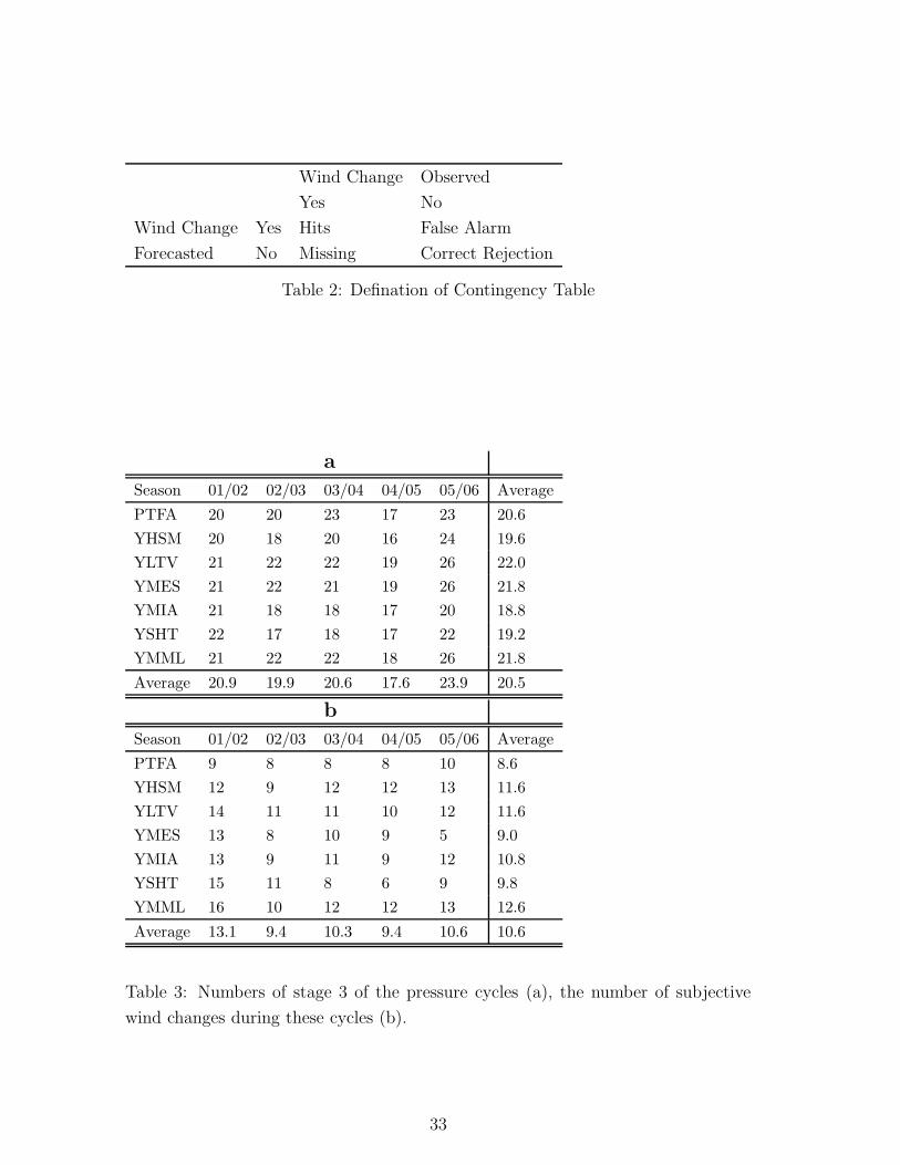
Wind Change Observed
Yes No
Wind Change Yes Hits False Alarm
Forecasted No Missing Correct Rejection
Table 2: Defination of Contingency Table
a
Season 01/02 02/03 03/04 04/05 05/06 Average
PTFA 20 20 23 17 23 20.6
YHSM 20 18 20 16 24 19.6
YLTV 21 22 22 19 26 22.0
YMES 21 22 21 19 26 21.8
YMIA 21 18 18 17 20 18.8
YSHT 22 17 18 17 22 19.2
YMML 21 22 22 18 26 21.8
Average 20.9 19.9 20.6 17.6 23.9 20.5
b
Season 01/02 02/03 03/04 04/05 05/06 Average
PTFA 9 8 8 8 10 8.6
YHSM 12 9 12 12 13 11.6
YLTV 14 11 11 10 12 11.6
YMES 13 8 10 9 5 9.0
YMIA 13 9 11 9 12 10.8
YSHT 15 11 8 6 9 9.8
YMML 16 10 12 12 13 12.6
Average 13.1 9.4 10.3 9.4 10.6 10.6
Table 3: Numbers of stage 3 of the pressure cycles (a), the number of subjective
wind changes during these cycles (b).
33
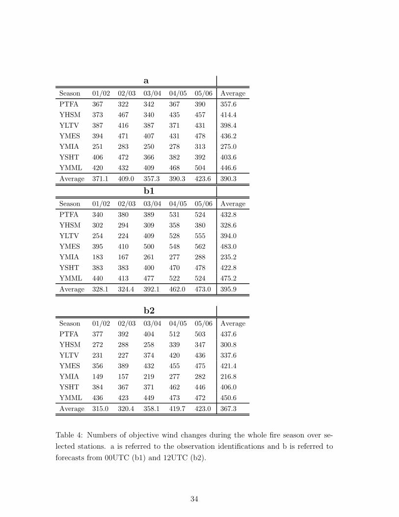
a
Season 01/02 02/03 03/04 04/05 05/06 Average
PTFA 367 322 342 367 390 357.6
YHSM 373 467 340 435 457 414.4
YLTV 387 416 387 371 431 398.4
YMES 394 471 407 431 478 436.2
YMIA 251 283 250 278 313 275.0
YSHT 406 472 366 382 392 403.6
YMML 420 432 409 468 504 446.6
Average 371.1 409.0 357.3 390.3 423.6 390.3
b1
Season 01/02 02/03 03/04 04/05 05/06 Average
PTFA 340 380 389 531 524 432.8
YHSM 302 294 309 358 380 328.6
YLTV 254 224 409 528 555 394.0
YMES 395 410 500 548 562 483.0
YMIA 183 167 261 277 288 235.2
YSHT 383 383 400 470 478 422.8
YMML 440 413 477 522 524 475.2
Average 328.1 324.4 392.1 462.0 473.0 395.9
b2
Season 01/02 02/03 03/04 04/05 05/06 Average
PTFA 377 392 404 512 503 437.6
YHSM 272 288 258 339 347 300.8
YLTV 231 227 374 420 436 337.6
YMES 356 389 432 455 475 421.4
YMIA 149 157 219 277 282 216.8
YSHT 384 367 371 462 446 406.0
YMML 436 423 449 473 472 450.6
Average 315.0 320.4 358.1 419.7 423.0 367.3
Table 4: Numbers of objective wind changes during the whole fire season over se-
lected stations. a is referred to the observation identifications and b is referred to
forecasts from 00UTC (b1) and 12UTC (b2).
34

a
Season 01/02 02/03 03/04 04/05 05/06 Average
PTFA 79 73 86 71 85 78.8
YHSM 85 78 67 67 100 79.4
YLTV 82 88 88 69 91 83.6
YMES 67 79 79 53 100 75.6
YMIA 51 53 48 52 67 54.2
YSHT 70 59 51 52 67 59.8
YMML 104 90 77 84 120 95.0
Average 76.9 74.3 70.9 64.0 90.0 75.2
b1
Season 01/02 02/03 03/04 04/05 05/06 Average
PTFA 73 88 91 87 115 90.8
YHSM 85 70 76 73 112 83.2
YLTV 59 61 81 92 129 84.4
YMES 71 85 90 78 105 85.8
YMIA 63 41 52 60 74 58.0
YSHT 83 53 72 81 111 80.0
YMML 87 78 85 88 117 91.0
Average 74.4 68.0 78.1 79.9 109.0 81.9
b2
Season 01/02 02/03 03/04 04/05 05/06 Average
PTFA 79 84 96 76 98 86.6
YHSM 70 64 52 58 91 67.0
YLTV 44 52 62 78 96 66.4
YMES 54 66 64 79 85 69.6
YMIA 46 41 36 51 59 46.6
YSHT 85 56 58 70 93 72.4
YMML 73 77 71 71 97 77.8
Average 64.4 62.9 62.7 69.0 88.4 69.5
Table 5: Same as Table 4 but restricted to periods of the pressure cycles listed in
Table 3.
35
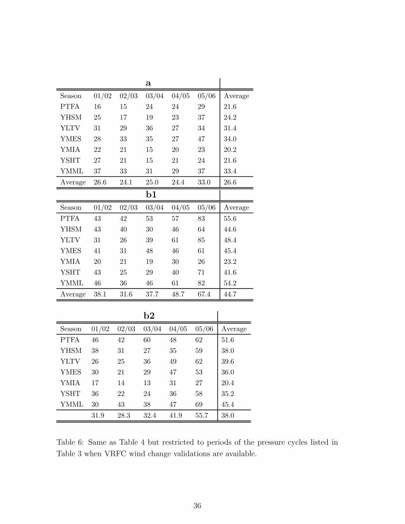
a
Season 01/02 02/03 03/04 04/05 05/06 Average
PTFA 16 15 24 24 29 21.6
YHSM 25 17 19 23 37 24.2
YLTV 31 29 36 27 34 31.4
YMES 28 33 35 27 47 34.0
YMIA 22 21 15 20 23 20.2
YSHT 27 21 15 21 24 21.6
YMML 37 33 31 29 37 33.4
Average 26.6 24.1 25.0 24.4 33.0 26.6
b1
Season 01/02 02/03 03/04 04/05 05/06 Average
PTFA 43 42 53 57 83 55.6
YHSM 43 40 30 46 64 44.6
YLTV 31 26 39 61 85 48.4
YMES 41 31 48 46 61 45.4
YMIA 20 21 19 30 26 23.2
YSHT 43 25 29 40 71 41.6
YMML 46 36 46 61 82 54.2
Average 38.1 31.6 37.7 48.7 67.4 44.7
b2
Season 01/02 02/03 03/04 04/05 05/06 Average
PTFA 46 42 60 48 62 51.6
YHSM 38 31 27 35 59 38.0
YLTV 26 25 36 49 62 39.6
YMES 30 21 29 47 53 36.0
YMIA 17 14 13 31 27 20.4
YSHT 36 22 24 36 58 35.2
YMML 30 43 38 47 69 45.4
31.9 28.3 32.4 41.9 55.7 38.0
Table 6: Same as Table 4 but restricted to periods of the pressure cycles listed in
Table 3 when VRFC wind change validations are available.
36

List of Figures
1 Example of wind change chart issued by the Victoria Regional Forecast
Center (From Kevin Parkyn, VRFC, personal communication). . . . . . . . 41
2 A schematic showing the conceptual structure of the cool change used in
the objective timing decisions. tsc is for wind change start time and tec is
for end change time. tds and tde are the time just before and after change
state. tmx is time when WCRI is maximum (after HM06). . . . . . . . . . . 41
3 Schematic showing the relationship between WCRI, WCSI, and WCDI (af-
ter HM06). The arrow in area 2 indicates the strengthening direction of
WCDI . . . . . . . . . . . . . . . . . . . . . . . . . . . . . . . . . . . . . . . 42
4 Schematic showing the conceptual model of 6 stages within a major pressure
change cycle. Stage 1: after high pressure; Stage 2: sub cycle after low
pressure; Stage 3: minimum low passage; Stage 4: rising pressure after
the lowest pressure; Stage 5: sub cycle high pressure; Stage 6: under the
influence of a major high-pressure system (after Huang and Mills, 2007). . . 43
5 Variations in WCRI with rate of change of direction for various speed
ranges, using the functions applied to numerical model data. . . . . . . . . 44
6 Example of the forecast WCRI, overlaid on the 10 m wind forecast, from
the Meso-LAPS05 forecast model. . . . . . . . . . . . . . . . . . . . . . . . 45
7 Map showing locations of Automatic Weather Stations in southeastern Aus-
tralia used in the study. The shading indicates the model topography. . . . 46
8 Verification statistics for VRFC wind change days. The left panels stratify
the data according to verification station, while the right panels stratify
according to fire season. The upper pair compare the observed objective
wind change times with the VRFC wind change times, with the green bars
showing the percentage of events for which the VRFC time is covered by
the extending observed wind change period, while the red bars show the
percentage of events for which the observed and subjective times are within
2.5 hours. Middle panels are in the same form, but comparing forecast
wind change periods and times with the VRFC times. Lower panels com-
pare model forecast and objective wind change periods and timings. Black
bars show the proportion of VRFC wind change days for which observed
and forecast wind change periods overlap, red bars show the proportion of
forecasts within 2.5 hours of the observed time, and the green bars show
the proportion of forecast wind change times that fall within the objective
wind change period. The numbers to the left of each set of 3 bars show
the number of events, and the sets of three numbers to the right show the
number of events in each of the three classes with the same colour codes. . 47
37
9 Scatterplots of wind change timing error versus forecast lead time for VRFC
wind change days, with the lower panels showing the smoothed mean and
standard deviation of error. In the right hand panel only those forecast
with errors less than 2.5 hours are shown. . . . . . . . . . . . . . . . . . . . 48
10 Contingency tables for all stage 3 pressure cycle changes. A hit means that
a wind change was diagnosed in both model and observations during that
pressure cycle stage. A missed forecast is counted if there is an observed
but not a forecast wind change, a false alarm if a change is forecast but
not observed, and a correct rejection if no change is either observed or
forecast in that stage. The numbers to the left of the bar show the total
number of stage 3 pressure cycles observed, and the numbers to the right
are colour-coded to indicate the numbers in each classification. . . . . . . . 48
11 Verification statistics for all matched forecast wind changes in stage 3 of
the pressure cycle. Black bars show the proportion of overlapped obser-
vation and forecast wind change periods, red bars show the proportion of
forecasts within 2.5 hours of the observed time, and the green bars show
the proportion of forecast wind change times that fall within the objective
wind change period. The numbers to the left of each set of 3 bars show
the number of events, and the sets of three numbers to the right show the
number of events in each of the three classes with the same colour codes. . 49
12 Scatterplot of wind change timing error versus forecast lead time for all
matched wind changes occurring in stage 3 pressure cycle phases, with the
lower panels showing the smoothed mean and standard deviation of error.
In the right hand panel only those forecast with errors less than 2.5 hours
are shown. . . . . . . . . . . . . . . . . . . . . . . . . . . . . . . . . . . . . 50
13 Case 1: mean sea level pressure analyses at 1200 UTC of 10 (a), 0000 UTC
of 11 (b) and 1200 UTC of 11 (c) March 2002. . . . . . . . . . . . . . . . . 51
14 Case 1: time series of meteorological variables at selected surface stations.
Vertical bars indicate the wind change identified from the observation (green
thin bar), the forecast (green thick bar) and the VRFC (blue bar). The
corresponding horizontal bars indicate the time spans of the wind change
period for the observation and forecast respectively. . . . . . . . . . . . . . . 52
15 Case 1: time series of meteorological variables at selected surface stations.
Vertical bars indicate the wind change identified from the observation (green
thin bar), the model forecast (green thick bar) and the VRFC (blue bar).
The corresponding horizontal bars indicate the time spans of the wind
change period for the observation and forecast respectively (continued). . . 53
16 Case 1: The forecasts of reduced sea surface pressure (a) and near surface
potential temperature (b) at 6 (1), 12 (2), 18 (3) and 21 (4) forecasting
hours, respectively. . . . . . . . . . . . . . . . . . . . . . . . . . . . . . . . . 54
38

17 Case 1: The 24-hour forecasts (1) and the corresponded analysis (2) of
reduced sea surface pressure (a) and surface potential temperature (b). . . . 55
18 Case 2: mean sea level pressure analyses at 1200 UTC, 1 NOV (a) and 0000
UTC, 2 Nov, 2004 (b). . . . . . . . . . . . . . . . . . . . . . . . . . . . . . . 56
19 Case 2: time series of meteorological variables at selected surface stations.
Vertical bars indicate the wind change identified from the observation (green
thin bar), the model forecast (green thick bar) and the VRFC (blue bar).
The corresponding horizontal bars indicate the time spans of the wind
change period for the observation and forecast respectively. . . . . . . . . . 57
20 Case 2: time series of meteorological variables at selected surface stations.
Vertical bars indicate the wind change identified from the observation (green
thin bar), the model forecast (green thick bar) and the VRFC (blue bar).
The corresponding horizontal bars indicate the time spans of the wind
change period for the observation and forecast respectively (continued). . . 58
21 Case 2: The second front passage. a is referred the reduced sea level pressure
and b is referred to the near surface potential temperature. The sequences
are shown at 1800 UTC (5 AM ADST) 1 Nov 2004 when the trough is off
the coast (1), 2200 UTC (9 AM ADST) when the trough first moves to
coast (2) and 2400 UTC (11 AM ADST) when the trough is further inland
(3). . . . . . . . . . . . . . . . . . . . . . . . . . . . . . . . . . . . . . . . . . 59
22 Case 3: mean sea level pressure analyses at 0000 UTC (a) and 1200 UTC
(b) 26 Jan, 2006. . . . . . . . . . . . . . . . . . . . . . . . . . . . . . . . . . 60
23 Case 3: a is referred the reduced sea level pressure and b is referred to the
near surface potential temperature. The sequences are shown at 1800 UTC
(5 AM ADST) 1 Nov 2004 when the trough is off the coast (1), 2200 UTC
(9 AM ADST) when the trough first moves to coast (2) and 2400 UTC (11
AM ADST) when the trough is further inland (3). . . . . . . . . . . . . . . 61
24 Case 3: time series of meteorological variables at selected surface stations.
Vertical bars indicate the wind change identified from the observation (green
thin bar), the model forecast (green thick bar) and the VRFC (blue bar).
The corresponding horizontal bars indicate the time spans of the wind
change period for the observation and forecast respectively. . . . . . . . . . 62
25 Case 3: time series of meteorological variables at selected surface stations.
Vertical bars indicate the wind change identified from the observation (green
thin bar), the model forecast (green thick bar) and the VRFC (blue bar).
The corresponding horizontal bars indicate the time spans of the wind
change period for the observation and forecast respectively (continued). . . 63
26 Case 4: mean sea level pressure analyses at 0000 UTC (a), 0600 UTC (b)
and 1200 UTC (c) on 29 Dec, 2001. . . . . . . . . . . . . . . . . . . . . . . . 64
39
27 Case 4: time series of meteorological variables. Vertical bars indicate the
wind change identified from the observation (green thin bar), the model
forecast (green thick bar) and the VRFC (blue bar). The corresponding
horizontal bars indicate the time spans of the wind change period for the
observation and forecast respectively. . . . . . . . . . . . . . . . . . . . . . . 65
28 Case 4: time series of meteorological variables. Vertical bars indicate the
wind change identified from the observation (green thin bar), the model
forecast (green thick bar) and the VRFC (blue bar). The corresponding
horizontal bars indicate the time spans of the wind change period for the
observation and forecast respectively (continued). . . . . . . . . . . . . . . . 66
29 Case 4: The forecasts of reduced sea surface pressure (a) and near surface
potential temperature (b) at 12 (1), 16 (2), 20 (3) and 24 (4) forecasting
hours, respectively . . . . . . . . . . . . . . . . . . . . . . . . . . . . . . . . 67
40
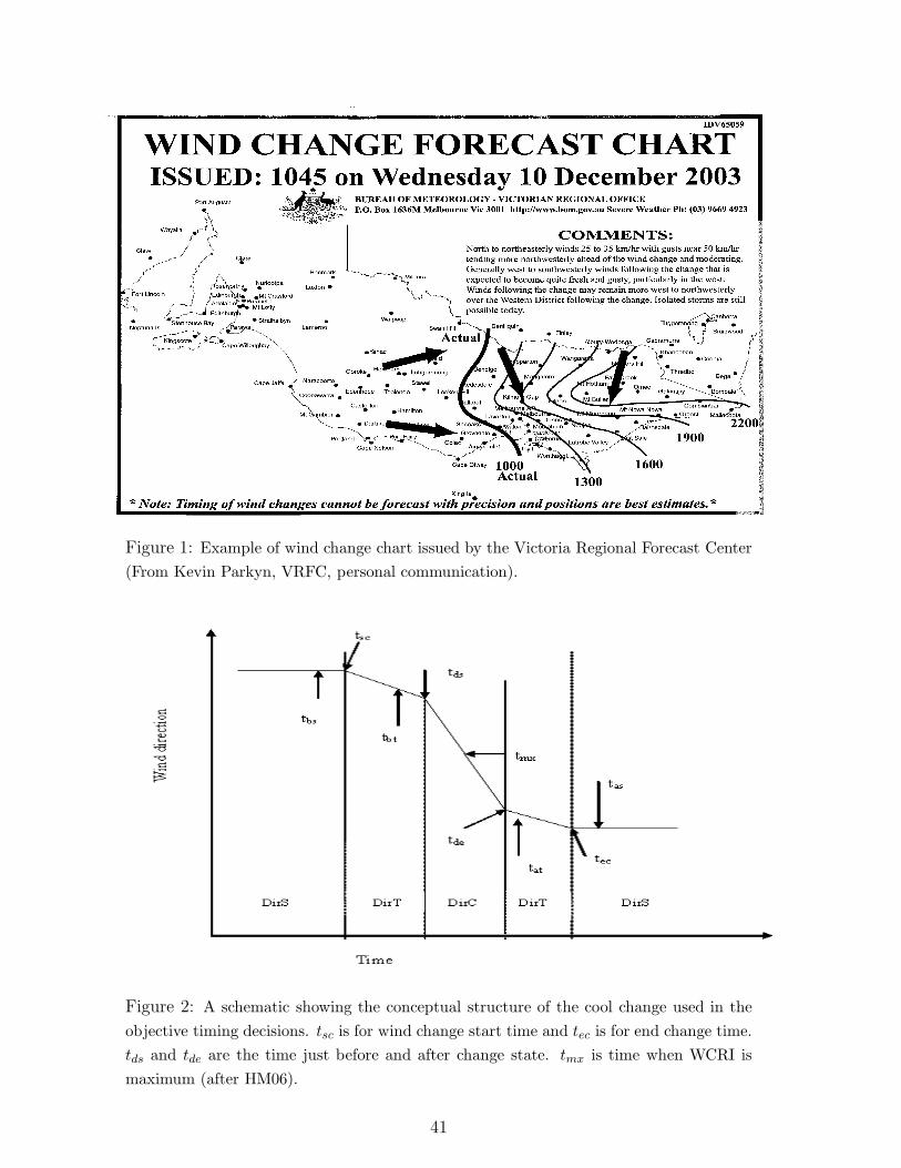
Figure 1: Example of wind change chart issued by the Victoria Regional Forecast Center
(From Kevin Parkyn, VRFC, personal communication).
Figure 2: A schematic showing the conceptual structure of the cool change used in the
objective timing decisions. tsc is for wind change start time and tec is for end change time.
tds and tde are the time just before and after change state. tmx is time when WCRI is
maximum (after HM06).
41
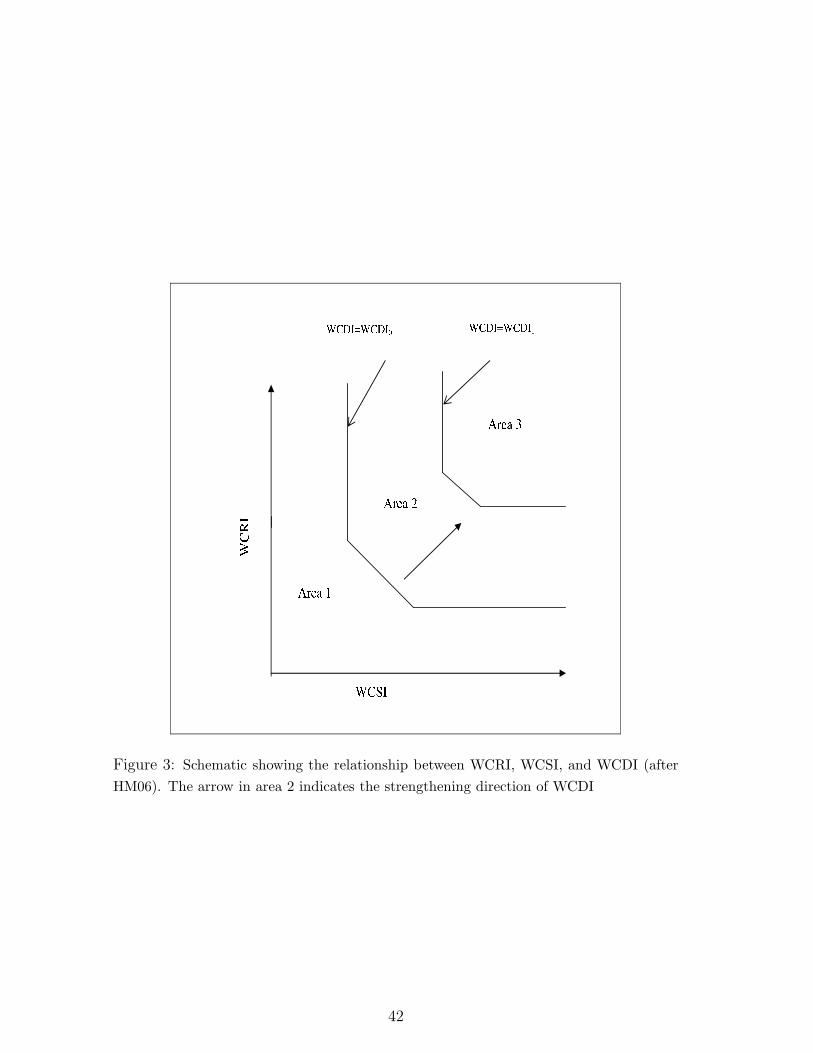
Figure 3: Schematic showing the relationship between WCRI, WCSI, and WCDI (after
HM06). The arrow in area 2 indicates the strengthening direction of WCDI
42

Figure 4: Schematic showing the conceptual model of 6 stages within a major pressure
change cycle. Stage 1: after high pressure; Stage 2: sub cycle after low pressure; Stage
3: minimum low passage; Stage 4: rising pressure after the lowest pressure; Stage 5: sub
cycle high pressure; Stage 6: under the influence of a major high-pressure system (after
Huang and Mills, 2007).
43
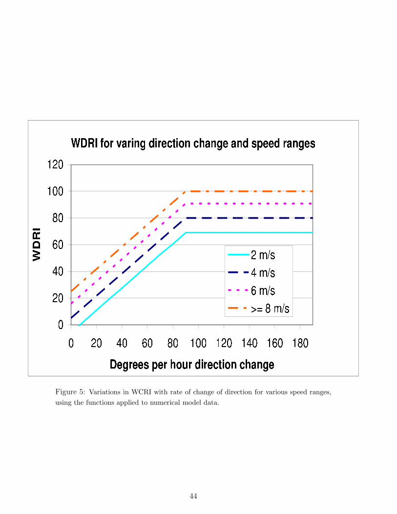
Figure 5: Variations in WCRI with rate of change of direction for various speed ranges,
using the functions applied to numerical model data.
44

Figure 6: Example of the forecast WCRI, overlaid on the 10 m wind forecast, from the
Meso-LAPS05 forecast model.
45

Figure 7: Map showing locations of Automatic Weather Stations in southeastern Australia
used in the study. The shading indicates the model topography.
46

1a, 2a
1b, 2b
3a 3b
Figure 8: Verification statistics for VRFC wind change days. The left panels stratify
the data according to verification station, while the right panels stratify according to fire
season. The upper pair compare the observed objective wind change times with the VRFC
wind change times, with the green bars showing the percentage of events for which the
VRFC time is covered by the extending observed wind change period, while the red bars
show the percentage of events for which the observed and subjective times are within 2.5
hours. Middle panels are in the same form, but comparing forecast wind change periods
and times with the VRFC times. Lower panels compare model forecast and objective wind
change periods and timings. Black bars show the proportion of VRFC wind change days
for which observed and forecast wind change periods overlap, red bars show the proportion
of forecasts within 2.5 hours of the observed time, and the green bars show the proportion
of forecast wind change times that fall within the objective wind change period. The
numbers to the left of each set of 3 bars show the number of events, and the sets of three
numbers to the right show the number of events in each of the three classes with the same
colour codes.
47
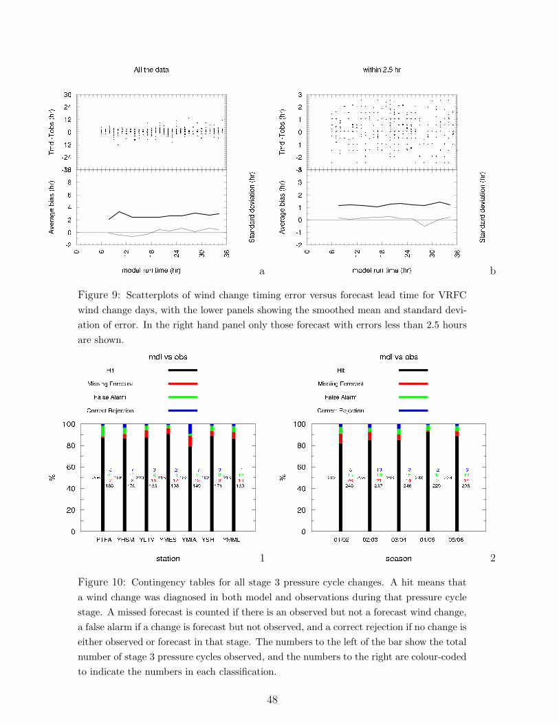
a b
Figure 9: Scatterplots of wind change timing error versus forecast lead time for VRFC
wind change days, with the lower panels showing the smoothed mean and standard devi-
ation of error. In the right hand panel only those forecast with errors less than 2.5 hours
are shown.
1 2
Figure 10: Contingency tables for all stage 3 pressure cycle changes. A hit means that
a wind change was diagnosed in both model and observations during that pressure cycle
stage. A missed forecast is counted if there is an observed but not a forecast wind change,
a false alarm if a change is forecast but not observed, and a correct rejection if no change is
either observed or forecast in that stage. The numbers to the left of the bar show the total
number of stage 3 pressure cycles observed, and the numbers to the right are colour-coded
to indicate the numbers in each classification.
48
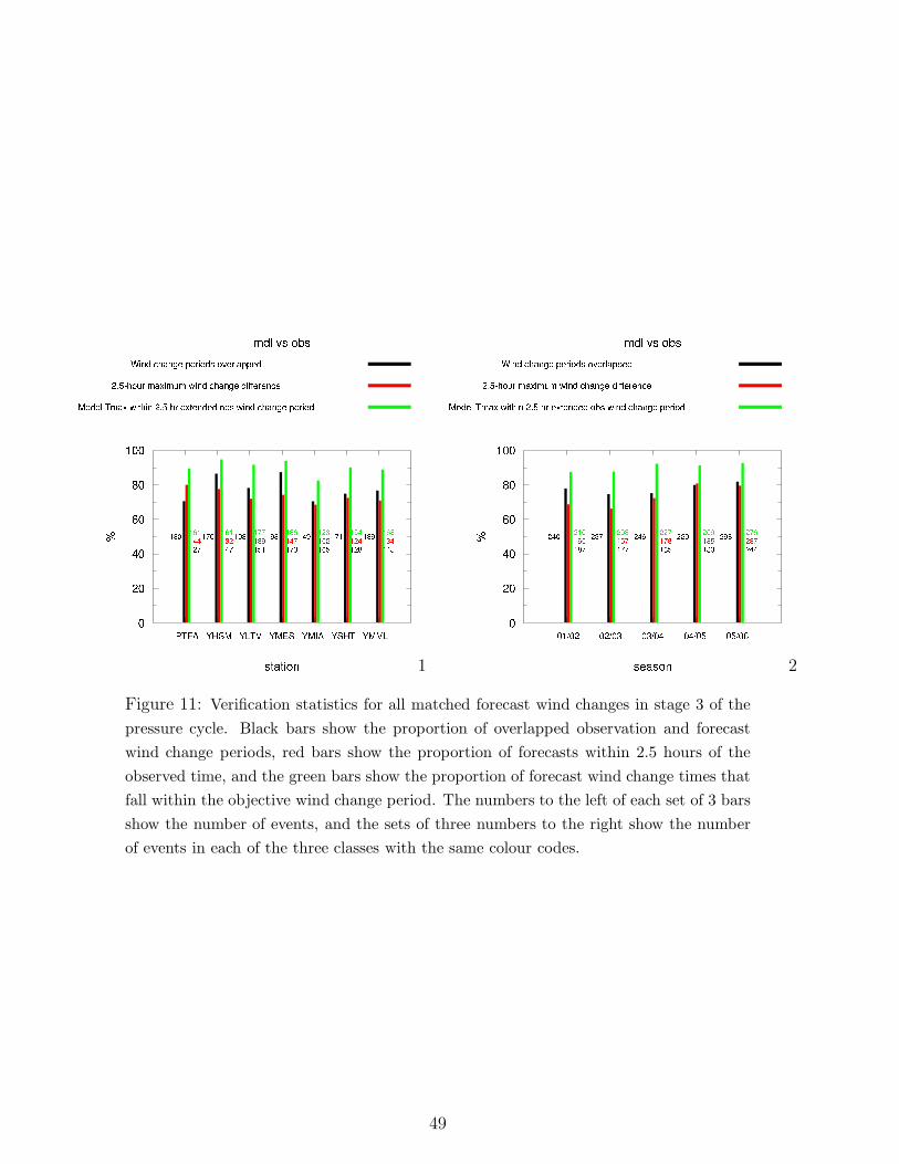
1 2
Figure 11: Verification statistics for all matched forecast wind changes in stage 3 of the
pressure cycle. Black bars show the proportion of overlapped observation and forecast
wind change periods, red bars show the proportion of forecasts within 2.5 hours of the
observed time, and the green bars show the proportion of forecast wind change times that
fall within the objective wind change period. The numbers to the left of each set of 3 bars
show the number of events, and the sets of three numbers to the right show the number
of events in each of the three classes with the same colour codes.
49
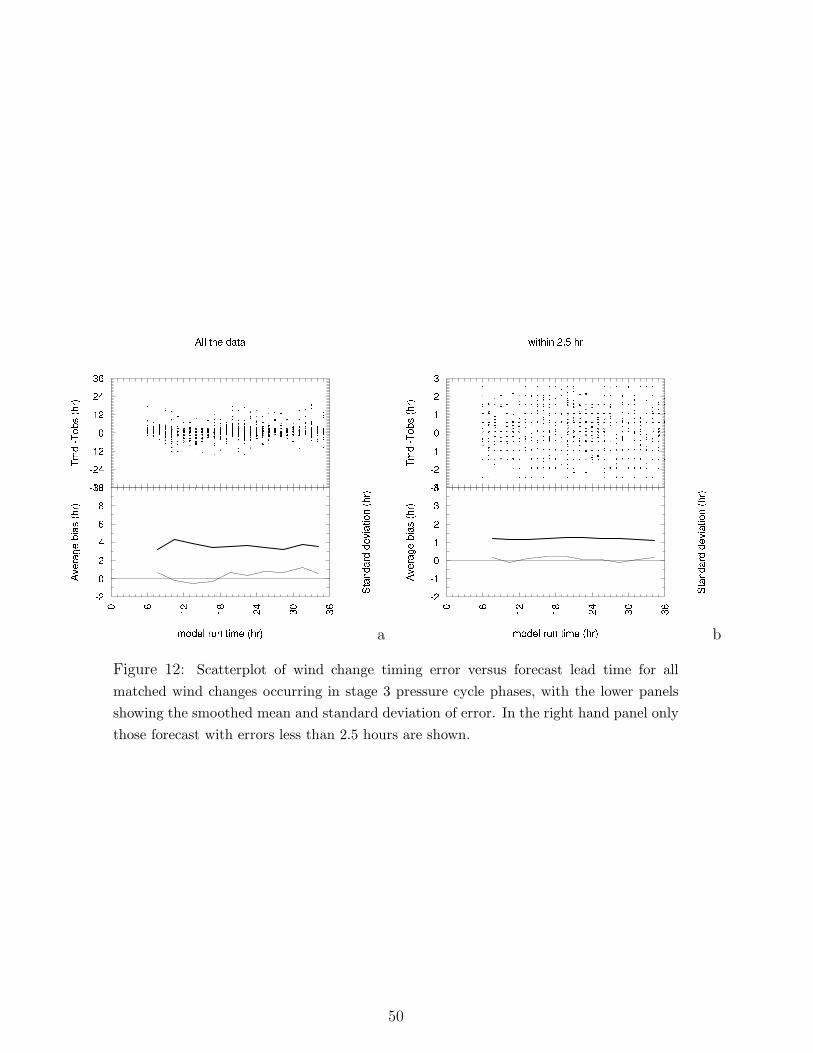
a b
Figure 12: Scatterplot of wind change timing error versus forecast lead time for all
matched wind changes occurring in stage 3 pressure cycle phases, with the lower panels
showing the smoothed mean and standard deviation of error. In the right hand panel only
those forecast with errors less than 2.5 hours are shown.
50
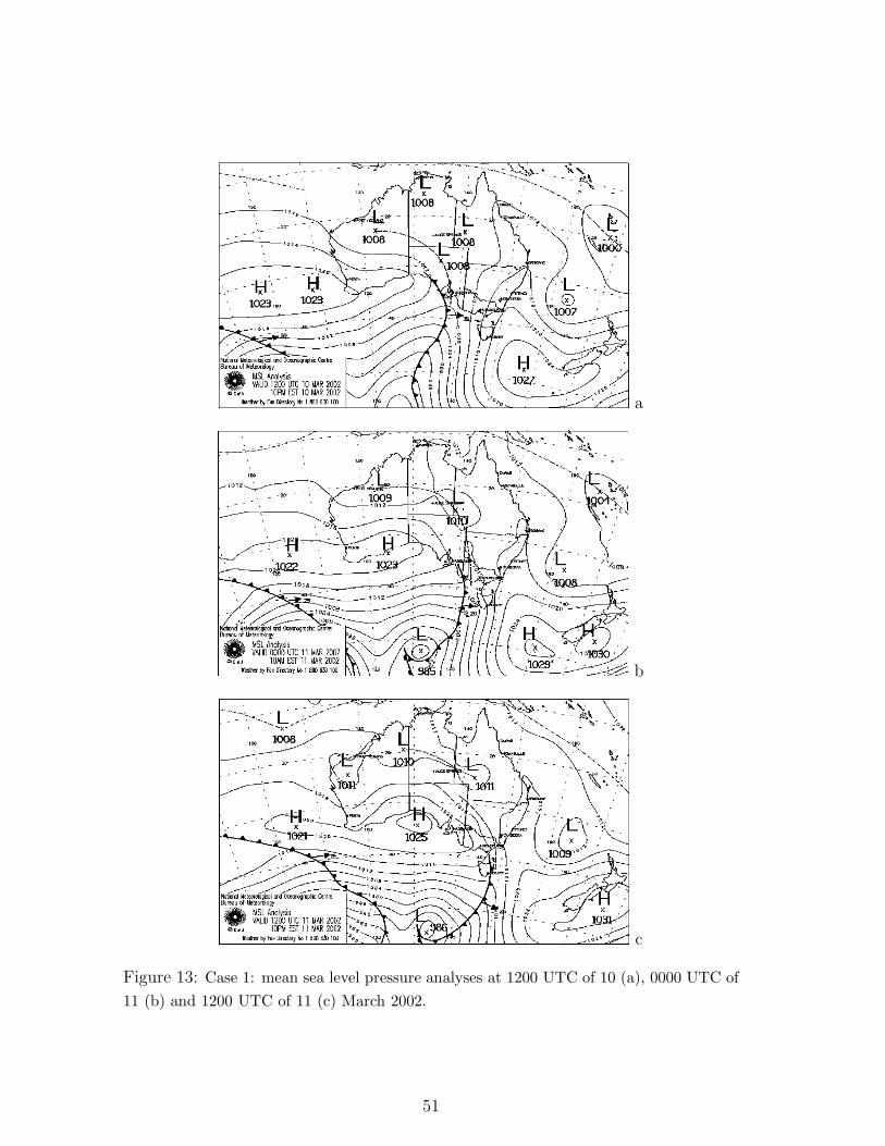
a
b
c
Figure 13: Case 1: mean sea level pressure analyses at 1200 UTC of 10 (a), 0000 UTC of
11 (b) and 1200 UTC of 11 (c) March 2002.
51
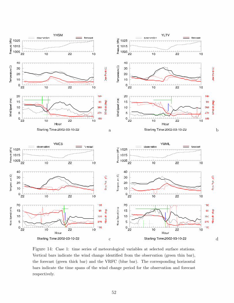
a b
c d
Figure 14: Case 1: time series of meteorological variables at selected surface stations.
Vertical bars indicate the wind change identified from the observation (green thin bar),
the forecast (green thick bar) and the VRFC (blue bar). The corresponding horizontal
bars indicate the time spans of the wind change period for the observation and forecast
respectively.
52

a b
c
Figure 15: Case 1: time series of meteorological variables at selected surface stations.
Vertical bars indicate the wind change identified from the observation (green thin bar), the
model forecast (green thick bar) and the VRFC (blue bar). The corresponding horizontal
bars indicate the time spans of the wind change period for the observation and forecast
respectively (continued).
53

a1 b1
a2 b2
a3 b3
a4 b4
Figure 16: Case 1: The forecasts of reduced sea surface pressure (a) and near surface
potential temperature (b) at 6 (1), 12 (2), 18 (3) and 21 (4) forecasting hours, respectively.
54

a1 a2
b1 b2
Figure 17: Case 1: The 24-hour forecasts (1) and the corresponded analysis (2) of reduced
sea surface pressure (a) and surface potential temperature (b).
55
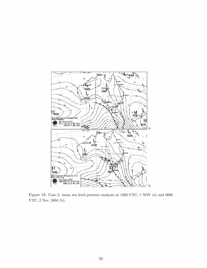
a
b
Figure 18: Case 2: mean sea level pressure analyses at 1200 UTC, 1 NOV (a) and 0000
UTC, 2 Nov, 2004 (b).
56

a b
c d
Figure 19: Case 2: time series of meteorological variables at selected surface stations.
Vertical bars indicate the wind change identified from the observation (green thin bar), the
model forecast (green thick bar) and the VRFC (blue bar). The corresponding horizontal
bars indicate the time spans of the wind change period for the observation and forecast
respectively.
57

a b
c
Figure 20: Case 2: time series of meteorological variables at selected surface stations.
Vertical bars indicate the wind change identified from the observation (green thin bar), the
model forecast (green thick bar) and the VRFC (blue bar). The corresponding horizontal
bars indicate the time spans of the wind change period for the observation and forecast
respectively (continued).
58

a1 b1
a2 b2
a3 b3
Figure 21: Case 2: The second front passage. a is referred the reduced sea level pressure
and b is referred to the near surface potential temperature. The sequences are shown at
1800 UTC (5 AM ADST) 1 Nov 2004 when the trough is off the coast (1), 2200 UTC (9
AM ADST) when the trough first moves to coast (2) and 2400 UTC (11 AM ADST) when
the trough is further inland (3).
59

a
b
Figure 22: Case 3: mean sea level pressure analyses at 0000 UTC (a) and 1200 UTC (b)
26 Jan, 2006.
60
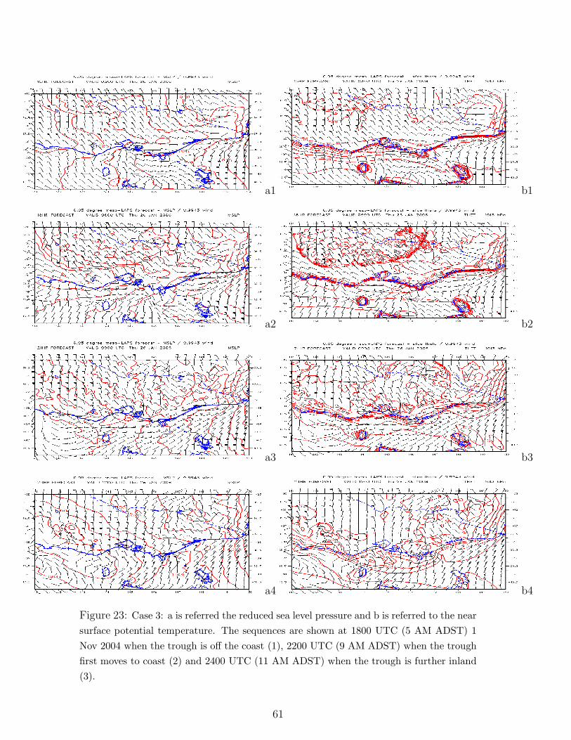
a1 b1
a2 b2
a3 b3
a4 b4
Figure 23: Case 3: a is referred the reduced sea level pressure and b is referred to the near
surface potential temperature. The sequences are shown at 1800 UTC (5 AM ADST) 1
Nov 2004 when the trough is off the coast (1), 2200 UTC (9 AM ADST) when the trough
first moves to coast (2) and 2400 UTC (11 AM ADST) when the trough is further inland
(3).
61

a b
c d
Figure 24: Case 3: time series of meteorological variables at selected surface stations.
Vertical bars indicate the wind change identified from the observation (green thin bar), the
model forecast (green thick bar) and the VRFC (blue bar). The corresponding horizontal
bars indicate the time spans of the wind change period for the observation and forecast
respectively.
62

a
Figure 25: Case 3: time series of meteorological variables at selected surface stations.
Vertical bars indicate the wind change identified from the observation (green thin bar), the
model forecast (green thick bar) and the VRFC (blue bar). The corresponding horizontal
bars indicate the time spans of the wind change period for the observation and forecast
respectively (continued).
63

a
b
c
Figure 26: Case 4: mean sea level pressure analyses at 0000 UTC (a), 0600 UTC (b) and
1200 UTC (c) on 29 Dec, 2001.
64

a b
c d
Figure 27: Case 4: time series of meteorological variables. Vertical bars indicate the wind
change identified from the observation (green thin bar), the model forecast (green thick
bar) and the VRFC (blue bar). The corresponding horizontal bars indicate the time spans
of the wind change period for the observation and forecast respectively.
65

a b
Figure 28: Case 4: time series of meteorological variables. Vertical bars indicate the wind
change identified from the observation (green thin bar), the model forecast (green thick
bar) and the VRFC (blue bar). The corresponding horizontal bars indicate the time spans
of the wind change period for the observation and forecast respectively (continued).
66
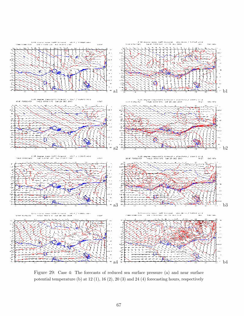
a1 b1
a2 b2
a3 b3
a4 b4
Figure 29: Case 4: The forecasts of reduced sea surface pressure (a) and near surface
potential temperature (b) at 12 (1), 16 (2), 20 (3) and 24 (4) forecasting hours, respectively
67


