
UNPACKING RURALITY Evaluating the impact of rural community characteristics and the built
environment on SNAP participation
Michele Walsh, Kara Tanoue & John Daws The Frances McClelland Institute for Children, Youth, and Families
The University of Arizona P.O. Box 210078
Tucson, AZ 85721-0078 Phone: 520-621-8739
Funded by a grant from the RIDGE (Research Innovation and Development Grants in Economics) Center for
Targeted Studies
December 2015

CONTENTS 1 Introduction .......................................................................................................................................... 1
2 Research Objectives .............................................................................................................................. 3
3 Methodology ......................................................................................................................................... 3
3.1 Study Area ..................................................................................................................................... 3
3.2 Data Sources ................................................................................................................................. 4
3.3 Data Processing ............................................................................................................................. 4
3.4 Variable Selection and Creation .................................................................................................... 5
3.5 Data Analysis ................................................................................................................................. 6
4 Results ................................................................................................................................................... 7
4.1 Cascade Analysis ........................................................................................................................... 7
4.2 Clustering ...................................................................................................................................... 9
5 Discussion ............................................................................................................................................ 10
5.1 Limitations and Future Directions ............................................................................................... 12
6 Tables and Figures............................................................................................................................... 13
7 References .......................................................................................................................................... 27
LIST OF TABLES Table 1. Six-Class Dasymetric Zone Classification ....................................................................................... 13
Table 2. Factors Used in Analysis ................................................................................................................ 14
Table 3. Cascade Analysis Results: Y1, Human Capital ............................................................................... 20
Table 4. Cascade Analysis Results: Y2, SNAP Drive Time ............................................................................ 21
Table 5. Cascade Analysis Results: Y3, Child SNAP Enrollment................................................................... 22
Table 6. Cascade Analysis Results: Y4, Relative Child SNAP Enrollment ..................................................... 23
Table 7. Cluster Descriptions ...................................................................................................................... 26
Table 8. Outcome variables by cluster ........................................................................................................ 26
LIST OF FIGURES Figure 1. Human Capital Factor .................................................................................................................. 16
Figure 2. Population-Weighted Mean Drive Time to a SNAP retailer ......................................................... 17
Figure 3. Estimated Percent of Children Enrolled in SNAP ......................................................................... 18
Figure 4.SNAP-Poverty Differential for Children (0-17) .............................................................................. 19
Figure 5. Cascade Analysis Direct Effects: Y1, Human Capital .................................................................... 20
Figure 6. Cascade Analysis Direct Effects: Y2, SNAP Drive Time ................................................................. 21
Figure 7. Cascade Analysis Direct Effects: Y3 Child SNAP Enrollment ........................................................ 22
Figure 8. Cascade Analysis Direct Effects: Y4, Relative Child SNAP Enrollment ......................................... 23
Figure 9.Total Cascade Analysis Effects ...................................................................................................... 24
Figure 10. Arizona Rural Clusters ................................................................................................................ 25

1
1 INTRODUCTION
A growing body of research has explored the impacts of the built environment on nutrition and health.
The built environment—human-constructed aspects of the physical environment such as transportation
infrastructure, land use and city design, and recreational facilities— has been shown to influence
physical activity, nutrition, and rates of obesity (Ball, K. et. al., 2005; Gordon-Larsen et al., 2006;
McKinnon et al., 2009; Sallis and Glanz, 2006; Simen-Kapeu et al., 2010). Many studies have focused
specifically on the availability of retail outlets selling healthy food within a certain “accessible”
geographic area as a significant determinant of healthy eating patterns (Burns et al., 2004, Hosler et al.,
2006; Larson et al., 2009; Walker et al., 2010). However, few studies have applied similar measures to
examine how participation in public assistance programs may be mediated by access.
Many of the earliest explorations of food environments and access arose out of the concept of a “food
desert,” a term first coined in the early 1990s (Cummins and Macintyre, 2002). The earliest definitions of
food deserts specified these regions as urban areas with few food retailers, in which access to healthy,
affordable food is highly limited (Cummins and MacIntyre, 2002; Hendrickson et al., 2006). The concept
of food deserts has since been expanded beyond the purely urban context to more generally denote
areas with poor access to food due to a general lack of food retailers or a lack of larger supermarkets
that provide a wider selection of more affordable food (Shaw, 2006; Ver Ploeg et al., 2009). However,
much of the newest and most innovative research regarding food access remains focused in urban
areas, due to ease of measurement and availability of data, despite the great needs for further research
in rural areas.
Rural areas and food access
Rural areas face special challenges in the realms of food access and health. Urban-rural health disparities
in obesity prevalence and nutrition have been widely acknowledged in the recent literature (Guy, 1991;
Larson et al., 2009; McKinnon et al., 2009; Simen-Kapeu et al., 2010). Simen-Kapeu et al. (2010) noted
that both Canadian and U.S. studies have found higher obesity and overweight prevalence in children
and youth living in rural environments (128). McKinnon et al. (2009), in a review of 137 articles
addressing food environments, similarly find that rural populations face higher risks of obesity and also
display greater sensitivities to environmental variables than non-rural populations, yet they found that
few instruments have been developed to measure food environments in strictly rural contexts (S129).
A number of the studies in rural areas have focused solely on the availability and cost of food in area
stores, reaching the same conclusion that food cost and availability are often compromised in rural
areas (Burns et al., 2004; Guy, 1991; Hosler et al., 2006; Liese et al., 2007; McEntee and Agyeman, 2010;
Yeager and Gatrell, 2014). Although studies of food availability across rural areas are important, few
studies of the built environment in rural regions consider variations within rural communities, instead
using rural as a monolithic identifier in opposition to urban communities (Boehmer et al., 2004; Burns et
al., 2004; Hosler et al., 2006; Liese et al., 2007; Sharkey and Horel, 2008; Simen-Kapeu et al., 2010). The
lack of exploration of intra-rural variation is problematic because knowing that an area is “rural” tells us
very little of the context of the community—the needs of a family in a small, well-established farming
town may have little in common with that of a family in a rather transient warm-winter haven along a
freeway. This project begins to fill the existing gap in studies of the rural built environment and food

2
access through the exploration of the impact of intra-rural cleavages and the built environment on
participation in Supplemental Nutrition Assistance Program (SNAP).
SNAP participation in rural areas
This project follows several recent explorations of social conditions surrounding SNAP participation and
health outcomes associated with program participation. Multiple studies have examined the impacts of
SNAP participation on childhood and adult obesity, finding that SNAP participation is often related to
high obesity and overweight prevalence across all age groups (Genser, 2009; Han et al., 2012; Leung et
al., 2013; Leung and Villamor, 2011; Simmons et al., 2012; Vartanian and Houser, 2012). Very few
studies have explored the impact of social and environmental factors on SNAP participation. Lacombe,
Michieka, and Gebremedhin (2012) use Bayesian spatial econometric modeling to study the influence of
key economic factors and immigration on SNAP participation in 417 Appalachian counties, finding that
poverty and employment exert the largest influence on SNAP participation. Leftin, Eslami, and Strayer
(2011), in a study of trends in SNAP participation by Mathematica Policy Research on behalf of the
USDA, found that SNAP participation remains highest among households with children and individuals
with the highest need and that participation rates were influenced by the economic downturn, changes
in benefits, and increased outreach. However, neither of these studies considered the influence of
additional social and community characteristics or the built environment on SNAP participation.
Addressing methodological challenges in studying rural areas
One of the continuing challenges of research into social and community characteristics in rural areas is
data acquisition and the need to move data between varyingly-defined spatial units. Commonly-termed
the “modifiable areal unit problem,” the arbitrary nature of the definitions of spatial units can confound
statistical analysis (Openshaw, 1984). Mennis (2003) notes the inherent problems associated with the
most commonly used small-area demographic datasets, such as the US Census, in that data are
aggregated to arbitrary areal units such as blocks, block groups, and census tracts (31). The use of such
units in geographic analysis assumes that the characteristics assigned to each unit are evenly distributed
across the area of that unit, when the true distribution may be quite uneven due to both natural and
built physical features such as lakes, mountain slopes, and patterns of land use (ibid.).
J.K. Wright (1936), an early 20th century cartographer, popularized a method of areal interpolation
termed “dasymetric mapping.” In dasymetric mapping, physical characteristics of a geographic surface,
such as land zoning and topographic terrain, are derived from ancillary datasets. These are then used to
guide areal interpolation (conversion of spatial data from one set of units to another) to develop a
continuous data surface that more accurately represents a population distribution than a choropleth
map based on administrative areal units could (Eicher and Brewer, 2001; Mennis, 2003). Both Mennis
(2003) and Eicher and Brewer (2001) found that use of dasymetric mapping, guided by ancillary land use
data, to generate surfaces for socioeconomic and demographic variable distributions from the US
Census produced highly accurate raster surfaces with finer detail than is often achieved through
choropleth mapping. Dasymetric mapping approaches to area interpolations and remodeling of Census
data have become widely used in geographic and urban planning literature, particularly since 2004
(Petrov, 2008; Wu et al., 2005). Shannon (2014) demonstrated the utility of a dasymetric approach to
the specific study of SNAP benefit usage and food access.

3
This project uses these dasymetric mapping approaches and other quantitative methods to build upon
prior research into the factors influencing SNAP participation through an exploration of the impact of
rural community characteristics and retailer access on SNAP participation.
2 RESEARCH OBJECTIVES
There were two primary aims of this project. The first was to explore the relationship between
theoretically-specified socio-geographical rural community characteristics and SNAP participation and
how this relationship is mediated by access to SNAP-authorized retailers. Through the use of an
exploratory technique, sequential canonical analysis, we attempted to identify factors that lead some
communities to under-utilize SNAP.
The second aim was to develop a typology that could differentiate among rural areas based on these
community characteristics. This approach follows from work done by Scholz and Herrmann (2010) on
behalf of the European Union Rural Future Networks project to develop a typology of rural regions in
Europe, and from geodemographic segmentation systems already used widely in commercial marketing
(Spielman and Thill, 2008). Through the use of cluster analysis, we aimed to identify multiple discrete
categories of rural communities that can be used to better understand the varying needs of different
rural populations across a state.
By identifying socio-geographical indicators of SNAP utilization, and the communities where they cluster,
we hope to be able to better develop and target outreach programs to rural communities with greatest
need.
3 METHODOLOGY
3.1 STUDY AREA This study examines data for the rural population of the state of Arizona. For the purposes of this study,
we define the rural population as any persons not living in a Census designated urban area. Urban
areas, as defined by the US Census, are Census-designated places with populations greater than or equal
to 50,000 (USDA, 2007). We have chosen to use the Census definition of rural and urban due to the
limitations of county-based definitions to accurately capture the rural and urban populations of Arizona.
Due to the large size of Arizona’s counties, many counties are classed as metropolitan counties despite
possessing sizable rural populations. For example, according to the 2010 US Census in Yavapai and
Cochise counties, both classified as metropolitan by the USDA definition, approximately 35 percent of
the population lives outside an urban cluster and 60 percent of the population live outside a cluster with
a population of more than 50,000. Using the broader Census definition of rural allowed us to capture
greater variability within rural areas in the state. Based on this definition of rural, our study looks at a
population of approximately 1.3 million people that accounts for about 20 percent of the population of
the state of Arizona.
We chose to study the rural population of the state of Arizona because of our team’s extensive
experience working in the state’s rural communities through partnerships with many agencies and

4
community organizations across the state. The extensive network our team has cultivated in the state of
Arizona assisted in data acquisition and contextualization of results.
3.2 DATA SOURCES We drew data for this project from three existing datasets. Community demographic and socioeconomic
data were obtained at the Census tract level from the 2010 US Decennial Census and the 2008-2012
American Community Survey (ACS) Five-Year Estimates. Select community health indicators were drawn
from the Arizona Department of Health Services 2012 Primary Care Area Statistical Profiles. SNAP
participation data were acquired from the Arizona Department of Economic Security, which administers
SNAP benefits within the state of Arizona, by zip code.1
3.3 DATA PROCESSING Spatial data are often collected and aggregated to a variety of geographic statistical units. In this study,
the data obtained came at three different geographic unit scales: Census tract, zip codes, and Primary
Care Areas (PCAs), a statistical unit created by the Arizona Department of Health Services. Holt, Lo, and
Hodler (2004) suggest that dasymetric methods can be applied to re-aggregated geographic data
between differing boundary definitions with a satisfactory level of accuracy. Following their approach,
we used dasymetric mapping to generate raster data surfaces for the demographic and socioeconomic
variables drawn from the 2010 Decennial US Census and the American Community Survey (ACS) 2008-
2012 5 year-estimates as well as health variables from the Primary Care Area (PCA) Statistical Profiles
and the 2012 SNAP enrollment dataset. All of these data surfaces were re-aggregated to the census tract
level to ensure a consistent unit of analysis.
For the dasymetric mapping, a six-class model was created using land ownership data from the Bureau
of Land Management, land cover data from the United States Geologic Service National Land Cover
Dataset, and hydrologic, topographic, and infrastructure data from the Arizona State Land Department.
The study area was classified into six land types: unpopulated, vegetated public land, vegetated private
land, agricultural land, low-density developed land, and high-density developed land (see Table 1, page
13). We followed Mennis (2003) in developing population density fractions. A population density surface
for each selected variable was created from the original source data at the geographic level provided
(tract, zip code, or primary care area). The unpopulated land type was assigned a zero population
density a priori, but density fractions for the other five land types were generated for each variable
through the use of zonal statistics within each of Arizona’s fifteen counties to determine the average
variable population density within that zone by county. Following Mennis (2003), these average
densities were converted to density fractions using overlay, raster calculator, and zonal statistics
functions in ESRI ArcGIS. First, identity functions were used to create a composite geography of areal
units of analysis (i.e., tracts, zip codes, PCAs), land class zones, and counties. For an area t of zone k in
county c the population fraction (d) equals the average population density of that zone in county c
1 We had initially planned to obtain health and nutritional outcomes from the 2012 Behavioral Risk Factor Surveillance Survey (BRFSS), obtained through the Arizona Department of Health Services. However, in the course of the research, the 2012 BRFSS was found to have insufficient coverage of Arizona’s rural areas, precluding it from inclusion in our analysis. Unfortunately, 2014 data were not available in time to be processed for this report, and will be included in subsequent iterations of the models.

5
divided by the sum of all average population densities in county c. For that same area t, the area fraction
(g) equals the portion of area t that falls into zone k divided by the total area t multiplied by the total
number of zones. The population density fraction (f) for area t of zone k in county c equals the
population fraction (d) multiplied by the area fraction (g) divided by the sum of the products of the
population fractions multiplied by the area fractions for all areas within area t.
Raster data surfaces with a 30m pixel resolution were generated for all 30 input variables selected as
well as their population denominators in addition to six outcome variables. All data were re-aggregated
to the 2012 census tract level for analysis. Six census tracts containing several military bombing ranges
and wildlife refuges with a total population of 0 were excluded from analysis. The total N for the study
was 399 census tracts.
3.4 VARIABLE SELECTION AND CREATION Variable selection for our analysis was based on previous work around rural typology development,
geodemographic segmentation, and socio-biogeographical analysis. Scholz and Hermann (2010) in their
work on European rural typologies used primarily economic indicators. Spielman and Thill (2008) in
their work on geodemographic segmentation used indicators having to do with population age and
ethnicity, housing characteristics, and economic and educational attainment characteristics. Cabeza de
Baca and Figueredo (2014) developed an integrated model of human ecology that takes into account
both life history and social privilege paradigms in examining social outcomes. Their model draws on the
idea that slow life history (indicated in our models by higher life expectancies, lower birth rates, and
lower infant mortality) is an indicator of a more stable and predictable environment, which helps
contribute to the development of human capital and associated positive social outcomes in
communities.
We created ten indicators, from 30 selected input variables theoretically suggested by these approaches
to be social and community factors likely to impact health-related outcomes, which could be mediated
by access to food assistance. These variables were drawn from the American Community Survey and
decennial Census and PCA statistical profiles, and included two derived access variables. Some were
single items and some were composite indicators. The indicators included were population density
(single item), slow life history (composite), median age (single item), work engagement (single item),
economic sector (composite), income equality (composite), linguistic isolation (single item), migration
(composite), ethnicity (composite), and resource access (composite) (see Table 2, page 14). As noted
above, all indicators were at the 2012 census tract level, for an N of 399.
The two access variables making up resource access were generated using ESRI ArcGIS. The first,
distance to urban centers, was a measure of driving time to the nearest urban area with a population
greater than 50,000. The second was a measure of driving time to the nearest SNAP-authorized
retailer. SNAP-authorized retailer locations were obtained from the USDA SNAP retail locator as of
September 2013, and locations were validated using satellite imagery in Google Earth.
To create the access surfaces, a road network for all roads within the state of Arizona and a 50 mile
buffer around the state was buffered by four meters and converted to a raster surface with values
determined by the speed limits assigned to those roads. This road surface was converted to a cost
surface by inverting those speed limits so that they represented minutes per mile traveled. This cost
surface was then used to create a path distance surface using the ArcGIS Path Distance tool, which
6
calculates the accumulated cost to traverse a surface given a set of origin points. The resulting two
surfaces provided a continuous raster surface showing the estimated driving time to an urban center or
to a SNAP retailer. This method of measuring access is limited as it does not account for traffic
congestion, one-way streets, or other more complex navigational challenges, but for this analysis we felt
it provided a sufficient measure of both retailer access and remoteness from a major urban center.
In addition to SNAP drive time, five other outcome variables were created for use in a series of multiple
regressions examining the direct and indirect effect of social and community characteristics on SNAP
enrollment (referred to below as the cascade analysis) (see Table 2, page 14). The first of these, human
capital, was a composite factor capturing educational attainment, material wealth (e.g., home
ownership, home value, vehicle ownership, etc.), and income. Because SNAP is a means-based
assistance program, socioeconomic status should affect SNAP enrollment, and we wanted to control for
this effect as a major causal factor. The distribution of human capital across the state is shown in Figure
1, page 16. The other four variables related to SNAP enrollment. Estimated percentages of adults
enrolled in SNAP and children enrolled in SNAP were created by dividing the average monthly
enrollment numbers for 2012 for adults and children by the census population numbers of children and
adults. SNAP enrollment differential variables for adults and children were created by subtracting the
percentage of adults and the percentage of children living at or below 200 percent of the poverty level
from the estimated percentage enrolled in SNAP. These variables allowed us to assess SNAP enrollment
relative to the low-income population. Preliminary analyses suggested that factors related to adult
enrollment were likely to be different than those related to child enrollment. Because this study was
conceived of as an initial examination of the feasibility and utility of these methodological approaches,
for the purposes of interpretability, we opted to focus on child SNAP enrollment in our analyses
3.5 DATA ANALYSIS We undertook a multi-phase analysis of the re-aggregated data with two primary goals: 1) to identify
the relation of key rural characteristics with access to SNAP retailers and impact on SNAP participation,
and 2) to develop a rural typology that captures the variations between communities with these key
characteristics.
Our first phase involved the exploration of the influence of the chosen rural factors on retailer access
and SNAP participation by structuring a pattern of regressions referred to as a cascade model in
cognitive psychology (Demetriou, Christou, Spanoudis, & Platsidou, 2002). In a cascade model, a series
of multiple regressions is performed in which the multiple criterion (outcome) variables are analyzed
sequentially according to a hypothesized causal order.
Because these criterion variables are expected to causally influence each other (that is, the identified
socio-geographic indicators are hypothesized to influence human capital in a community and human
capital is likely to influence access, which is likely to influence nutrition assistance participation), they
are entered sequentially into a system of multiple regression equations with each hierarchically prior
criterion variable entered as the first predictor for the next. In this way, each successive criterion
variable is predicted from an initial predictor variable, each time entering the immediately preceding
criterion variable as the first predictor, then entering all the ordered predictors from the previous
regression equation. Each successive regression enters all of the preceding criterion variables in reverse
causal order, to statistically control for any indirect effects that might be transmitted through them.

7
Within this analytical scheme, the estimated effect of each predictor is limited to its direct effect on
each of the successive criterion variables.
Analogous to a Sequential Canonical Analysis (SEQCA), this kind of cascade model has been proposed to
serve as an exploratory form of path analysis (Figueredo & Gorsuch, 2007) where the exact model
specification cannot be completely predicted by existing theory. Formal Structural Equation Modeling
(SEM) would be unsuitable for the current study because SEM requires a complete model specification
based on strong a priori theory, whereas this work, though theoretically based, is exploratory in nature.
A cascade model therefore provides a theoretically-guided exploration rather than a formal and
confirmatory test of a priori theory, which is very appropriate in the context of this early work.
The general schematic format for this system of multiple regressions for this study was:
Y(HumanCapital)= β1 Socio-geographic (SG) Indicators
Y(Access)= β2 Y(HumanCapital) + β1 SGIndicators
Y(SNAP Enrollment)= β3 Y(Access) + β2 Y(HumanCapital) + β1 SGIndicators
Y(SNAP Differential)= β4 Y(SNAP Enrollment)+ β3 Y(Access) + β2 Y(HumanCapital) + β1 SGIndicators
We then used cluster analysis of the factors in the model to develop community clusters that served as
the basis for our rural community typology. Our use of cluster analysis follows work done by Scholz and
Herrmann (2010) on behalf of the European Union Rural Future Networks project that used k-means
cluster analysis to develop a typology of rural development regions in the European Union. Similar
techniques have long been used in marketing as a key component of geodemographic segmentation
systems, which aim to develop discrete categories of consumers based on behavior, demographic, and
lifestyle data by which small geographic areas can be classified (Spielman and Thill, 2008). We used k-
means clustering, an unsupervised learning technique, to develop clusters of rural communities from
which our typologies were drawn.
4 RESULTS
4.1 CASCADE ANALYSIS We ran the cascade analysis with four outcome variables: human capital (Y1), mean drive time to a SNAP
authorized retailer (Y2), estimated percent of children enrolled in SNAP (Y3), and child enrollment in
SNAP relative to low-income status (Y4). The results, with each criterion variable statistically controlled
in reverse order, are shown in Table 3 to Table 6, on pages 20-23 The overall pooled multivariate effect
size for the model was large (V=1.428, E=.6, F60,1532=14.18, p <.001).
In the first cascade, we predicted human capital from indicators selected to be likely to influence
socioeconomic well-being in rural areas. Higher resource access (sR=.38), percent white (sR=.14), income
equality (sR=.13), housing health (sR=.09), primary (sR=.16) or secondary (sR=.09) sector employment2,
work engagement (sR=.19), and higher median age of the census tract population (sR.10) were all
2 Primary-sector employment includes agriculture and mining; secondary-sector employment includes manufacturing and construction; tertiary-sector employment includes the service industry.

8
associated with higher levels of human capital. Linguistic isolation (sR=-.42), percent Hispanic or Latino
(sR=-.26), and percent non-Hispanic non-white (sR=-.25) were associated with lower levels of human
capital. (The effect sizes presented are semi-partial correlations. See Table 3 for additional details. A
schematic representation of the statistically significant direct effects are presented in Figure 5.)
In the second cascade, we predicted access (driving time) to SNAP retailers using the same indicators,
controlling for their relation via human capital. Here, we found that human capital (sR=-.24) was
significantly negatively correlated with mean drive time to a SNAP retailer (that is, tracts with higher
human capital tended to have lower drive time to retailers). In addition to the indirect effects some
variables had through human capital, resource access (sR=-.52), linguistic isolation (sR=-.21), percent
Hispanic or Latino (sR=-.09), percent non-white non-Hispanic (sR=-.08), tertiary (sR=-.15)and secondary
(sR=-.14) sector employment, work engagement (sR=-.09), and population density (sR=-.21) were also
directly significantly negatively correlated with SNAP drive time. (See Table 4, page 21 for additional
details. A schematic representation of the statistically significant direct effects are presented in Figure
6.)
In the third cascade, we predicted Census tract levels of child SNAP enrollment, based on estimates
obtained via dasymetric mapping. Human capital (sR=-.53) was significantly negatively correlated with
child SNAP enrollment (tracts with lower levels of human capital had a higher proportion of children
enrolled in SNAP), but there was no statistically significant relationship between SNAP drive time and
child SNAP enrollment. Even controlling for the effects through human capital, linguistic isolation
(sR=.13), all employment sectors (primary sR=.20; secondary sR=.10; tertiary sR=.11), median age
(sR=.09), and population density (sR=.41) were positively correlated with child SNAP enrollment.
Resource access (sR=-.08), percent non-white, non-Hispanic (sR=-.11), and work engagement (sR=-.08)
were negatively correlated with child SNAP enrollment. (See Table 5, page 22 for more details. A
schematic representation of the statistically significant direct effects are presented in Figure 7.)
In the fourth cascade, child SNAP enrollment (sR=.67) had a positive relationship with relative child
SNAP enrollment, meaning that as overall child enrollment increases, the gap between the percent of
children that are low-income and the percent of children enrolled in SNAP decreases. Also, human
capital (sR=.46) had a direct positive correlation, after partialling out the negative indirect effect through
its relationship with child SNAP enrollment. However, SNAP drive time (sR=-.18) was significantly
negatively correlated with relative child SNAP enrollment, suggesting that access to SNAP retailers does
have a mediating role in SNAP enrollment. In communities with poor access to SNAP retailers (higher
driving times to retailers), there are greater percentages of low income children who are not enrolled in
SNAP, even though there is no direct relationship with child SNAP enrollment. Percent non-white non-
Hispanic (sR=.08), income equality (sR=.14), work engagement (sR=.16), median age (sR=.12), and slow
life history (sR=.07) were significantly positively correlated with parity in child SNAP enrollment, even
after partialling out the effect through human capital and percent of SNAP enrollment where there was
one. Linguistic isolation (sR=-.07), percent Hispanic or Latino (sR=-.05), percent white (sR=-.08),
migration(sR=-.13), and primary-sector employment (sR=-.18) were significantly negatively correlated
with relative child SNAP enrollment. (See Table 6, page 23 for more details. A schematic representation
of the statistically significant direct effects are presented in Figure 8.)

9
4.2 CLUSTERING To increase interpretability of this data in order to make these results more easily actionable, we used k-
means clustering to create a typology of rural communities in Arizona based on our input variables and
our human capital factor. Because k-means clustering is an unsupervised learning method that does not
produce an outcome measure of fit or error, it is left to the experimenter to choose appropriate
clusters. As such, we ran multiple cluster analyses with differing allowed numbers of clusters, and chose
an eight-cluster set that was both interpretable and that had face validity with those working in these
rural communities in Arizona.
The clusters were named based on their relative levels of the variables included, and on other
characteristics of the areas (see Figure 10, page 25).
Ag/Mining/Forestry: This cluster encompassed areas of the state known for mining and agriculture. It
had the highest primary-sector employment and lowest tertiary-sector employment as well as low
population density.
Border City: This cluster encompassed the smallest tracts at the center of towns straddling the US-
Mexico border. It was characterized by high population density, high linguistic isolation, high migration,
high Hispanic population, and low housing capital.
Border Periphery: This cluster encompassed the tracts surrounding the border cities. It was
characterized by high migration, high Hispanic population, high primary-sector employment, and high
linguistic isolation.
Mixed Migrant: This cluster encompassed tracts widely spread across Arizona. It was the most ethnically
diverse cluster, with high migration and high primary- and secondary-sector employment as well.
Suburb/Historically Mormon: This cluster encompassed many of the tracts closest to major cities in
Arizona as well as a number of areas that were historically founded by Mormon settlers. This cluster
possessed the highest resource access, the highest income equality, the highest work engagement,
highest human capital, and the lowest primary-sector employment.
Retirees: This cluster encompassed the belt across central Arizona known for its snowbird population as
well as some of the major retirement destinations in the state. It had the highest median age, highest
white population and the slowest life history, while also being characterized by high human capital and
low work engagement.
Scenic: This cluster encompassed much of northern Arizona, including many popular locations for
vacation homes. It was characterized by high median age, the highest housing capital, high work
engagement, high secondary-sector employment, and a high proportion of white residents.
Tribal: This cluster encompassed the majority of the reservation lands within Arizona. It possessed the
highest non-white and non-Hispanic population with low migration, low median age, fast life history,
and low income equality.
The means and standard deviations of the four outcome variables by cluster are shown in Table 8,
ordered by percentage of child SNAP enrollment relative to child low income. As might be expected, the
clusters with the highest mean human capital (Retiree, Scenic and Mormon/Suburb), have the lowest

10
proportion of child SNAP enrollment. Four clusters have a greater than 10 percent disparity between
enrollment and low income: Tribal, Mixed Migrant, Border Periphery, and the Ag/Mining and Forestry
tracts. The clusters with the two highest drive times to SNAP retailers are represented (Tribal &
Ag/Mining/Forestry), as is the cluster with the lowest human capital (Tribal). In spite of its low ranking
on human capital, and high levels of SNAP enrollment, the mean Border City relative SNAP enrollment
was high, suggesting that a relatively high proportion of low-income children are enrolled in SNAP.
MANCOVA results showed a statistically significant effect of cluster on the SNAP indicators (Λ = .480,
F(35,1630) = 8.89, p<.01)
Looking at each of the criterion variables separately (in ANOVAs), there were significant differences by
cluster on each of the four measures, though the variance explained by cluster for relative child SNAP
enrollment is less than 10 percent (see Table 8, Page 26).
5 DISCUSSION
The objectives of this study were to explore factors that are related to SNAP enrollment in rural areas,
and to attempt to aggregate those factors in ways that differentiated among rural areas and are
actionable.
Our analyses show that the variables we have identified as likely to have an influence on SNAP
enrollment, and ultimately on health outcomes, had explanatory power and are interrelated in
theoretically interesting ways. The cascade models show that there are complicated relationships
among many of the variables that predict whether low income children in any particular rural area are
likely to be enrolled in SNAP.
For instance, population density is typically used as a measure of rurality, and as a proxy for a number of
facets of rurality such as economic development or resource access. We have shown that using a direct
measure of remoteness, such as driving time to an urban center and length of work commute, has a
strong direct relation to the level of human capital in an area, and through indirect effects, a stronger
relation to relative SNAP enrollment, than population density, per se. However, population density does
predict both drive time to SNAP retailer and estimated child SNAP enrollment even when accounting for
remoteness and other predictors of human capital. Considering both remoteness and density captures
a more nuanced sense of what is important about rurality.
Although access to a SNAP retailer does not directly predict a higher proportion of children enrolled in
SNAP within a community, the driving distance to a SNAP retailer does predict that a relatively lower
proportion of low-income children will be enrolled in SNAP. This demonstrates that access may be a
significant factor in mediating SNAP enrollment. Enrollment and educational outreach efforts should
include awareness by staff of the likely drive time to SNAP retailers in a community.
About 14 percent of the variance in relative SNAP enrollment was predicted by the direct effect of
indicators that had originally been hypothesized to be likely to show an effect on SNAP enrollment only
indirectly, through human capital. For instance, primary-sector employment (mining, forestry,
agriculture) has a direct negative effect on relative SNAP enrollment for children, over and above
economic sector effects on human capital, drive time to SNAP retailer and estimated child SNAP

11
enrollment. Ethnicity also had direct effects even after effects through the previous criterion variables
and linguistic isolation have been partialled out. As our previous work has suggested (Walsh, Katz &
Sechrest, 2002; Walsh, et al., 2000), ethnicity is not itself a causal factor, but represents, and often can
be accounted for by better measuring, the many facets that underlie it. Efforts to better understand
and measure the meaning of ethnicity in rural areas could be fruitful in better targeting SNAP outreach.
Two of our indicators did not have an indirect effect at all but only showed a significant direct effect on
relative SNAP enrollment: our migration indicator (which captured both international and intra-national
migration) and our slow life history variable (which captured fertility and mortality, theoretically related
to harsher environments). These indicators had an effect even after controlling for human capital,
access to SNAP retailers and estimated child SNAP enrollment, suggesting unique effects of these factors
that would be worth exploring through additional qualitative and quantitative work. It may be that
migration effects reflect both eligibility and informational barriers to enrollment. Slow life history is
theoretically related to higher levels of parental effort to provide resources for their children (e.g.
Cabeza de Baca et al., 2012), which is consistent with the findings here.
Overall, the results of the cascade model help to illustrate how important it is to consider multivariate
models that account for many of the variables affecting relative SNAP enrollment simultaneously, rather
than relying on bivariate descriptions of relationships. Unfortunately, as we described in the
introduction, efforts to develop multivariate models in rural areas are stymied by the challenge of
including data from varyingly-defined spatial units. Dasymetric mapping allowed us to produce a
consistent level of analysis (Census tract) for each of these variables and so to include more
sociogeographic variables than are typically available. We believe that this is a promising approach for
more refined rural analysis. As the amount of intra-county variability shown in our maps demonstrates,
this type of small area analysis is likely to result in a better understanding of rural populations and their
needs than is the more typical county-level analyses, especially in western areas where the geographic
size of counties can be vast.
As our ANOVAs showed, we were able to use cluster analysis to capture the variability of rural areas
across the indicator variables. The eight clusters were able to account for a statistically significant
proportion of the variance in each of our criterion variables, ranging from 47 percent of the variance in
Human Capital down to 8 percent of the variance in Relative Child SNAP Enrollment. The four clusters
lowest on Relative Child SNAP Enrollment (the Tribal, Mixed Migrant, Border Periphery, and
Ag/Mining/Forestry) were more than 10 percent lower than the others. Better outreach or other
interventions in these particular areas might increase the proportions of low-income children enrolled in
SNAP. The relatively low enrollment of low-income children in SNAP in Tribal clusters may be a feature
of an alternative food assistance option for people residing on Indian reservations: the Food Distribution
Program on Indian Reservations (FDPIR). The FDIR was established, in part, as a recognition of the
barrier to benefit use that the long distances to SNAP (then food stamp) retailers placed on reservation
residents (Finegold, et al., 2009). Although eligibility requirements are similar, households cannot
participate in both FDPIR and SNAP in the same month. A report comparing FDPIR and SNAP (Finegold,
et al., 2009) found that the size of the benefit that would be received by participants was typically larger
with SNAP, but that program staff and participants reported that ease of enrollment and cultural
compatibility favored FDPIR.

12
Importantly, we have begun to use the typology which the clusters form to engage with Cooperative
Extension agents and staff in thinking about the counties they work in. We have been met with
excitement about this approach, and have been given feedback that this way of considering and
documenting variability is more meaningful to those working in rural areas.
5.1 LIMITATIONS AND FUTURE DIRECTIONS Although this work was theoretically driven, it is exploratory in nature, and uses methodologically
innovative approaches that will need confirmation through various other studies. Therefore, even
though this study is a good starting point for unpacking rurality as it relates to SNAP usage, it is only a
beginning.
In particular, we want to avoid reifying the typology we have developed so far, but rather refine it by
developing targeted model comparisons and conducting sensitivity analyses. In order to do so, we
intend to continue to engage with stakeholders around the face validity and utility of the typology, and
to solicit their input for variables to include that would better capture and differentiate among the areas
they work in. Qualitative data from program participants would be helpful in better understanding
some of the barriers to enrollment and redemption in different areas, which would allow us to further
refine our variable selection. As a step towards developing a more robust typology, it would be useful to
go beyond k-means clustering and to incorporate methods of multivariate aggregation that allow for
assessing goodness of fit, such as latent class analyses. Because a useful typology should capture
variation across a number of related phenomena, as we continue to develop the typology, we will
explore its relationship with other variables, including enrollment and use of other social benefit
programs (such as WIC) and health outcomes.
Although we have used enrollment estimates in the current model, it would be useful to extend the
model to include redemption data. We would anticipate that SNAP retailer access would have even a
stronger effect on SNAP redemption. In the current model, we have treated all SNAP retailer types as
equivalent. (Types of SNAP retailers include supermarkets, small grocery stores, convenience stores,
farmers markets, and others.) In the future, we would like to use these techniques to explore the
influence of SNAP retailer types and changes in SNAP retailer access, enrollment and redemption over
time. It would also validate the influence of SNAP retailer access on SNAP enrollment by conducting
intervention studies that improve access to SNAP benefit redemption in areas identified as having
limited access. It is also important to recognize the limitations of secondary data when exploring barriers
to SNAP enrollment. The integration of qualitative data gathered from SNAP enrollees could greatly
enhance our understanding of the role that physical access plays in SNAP enrollment and participation.
The primary benefit of the approaches we have laid out is in the utility they offer to stakeholders in rural
areas. Having a concrete way to better understand and describe the variability in rural areas would aid
in stronger advocacy for the differing needs across rural populations. Although these techniques do not
fully account for the rich variation in culture and experience in rural communities, these methods go
beyond the standard way of presenting rural as a monolithic identifier that can mask the great diversity
of needs and assets in rural America.

13
6 TABLES AND FIGURES
Table 1. Six-Class Dasymetric Zone Classification
Dasymetric Zone Description
Unpopulated Land areas within 4 meters of a body of water, within 2 meters of a road or
highway, with a slope of greater than 30 degrees, falling within the footprint
of airports, golf courses, or parks, or classified as barren
Vegetated Public Land Publicly owned land (state or federal) classified as covered by forest, shrubs, or
grasses
Vegetated Private Land Privately owned land classified as covered by forest, shrubs, or grasses
Agricultural Land Private or publicly owned land classed as agricultural
Low Density Developed Land Private or publicly owned developed at low density
Mid-High Density Developed Land Private or publicly owned developed at medium or high density

14
Table 2. Factors Used in Analysis
Type
Variable Used in
Analysis Operationalization Source
Input
Population
Density
Total population per square kilometer U.S. Census 2010
Slow Life History Composite factor of birth rate per 1,000 population, fertility rate per
1,000 females ages 15-44, teen birth rate per 1,000 females ages 14-
19, percent premature mortality
ADHS PCA Profiles
Median Age Median age ACS 2008-2012
Work
Engagement
Percent of population ages 16 and over in the labor force ACS 2008-2012
Economic Sector Three composite factors of the percent of population ages 16 and over
employed in the following economic sectors: PRIMARY (Mining,
agriculture, forestry, hunting), SECONDARY (Construction,
manufacturing), TERTIARY (Service, retail, management, scientific,
administration)
ACS 2008-2012
Housing Health Composite factor of the reverse coded mean of non-seasonal vacancy
rate and median year built.
ACS 2008-2012
Income Equality Reverse-coded Gini coefficient, which measures the degree of
inequality in the income distribution within the census tract.
ACS 2008-2012
Linguistic
Isolation
Percent of households in which no one over the age of 14 speaks
English "very well"
ACS 2008-2012
Migration Composite factor of the percent of the population that is foreign born,
percent reporting non-citizenship, percent that lived in a different city
or town one year ago
ACS 2008-2012
Ethnicity Three composite factors of the percent of the population that is non-
Hispanic white (WHITE), Hispanic or Latino (HL), or non-white non-
Hispanic (OTHER)
ACS 2008-2012
Resource Access Composite factor of mean drive time to urban center and percent of
the population that commutes an hour or more to work by private
vehicle
Derived; ACS
2008-2012
Human Capital Composite factor of median household income, education attainment
(ordinal), employment rate, percent of population above the poverty
line, median home value, homeownership rate, percent of homes that
are not overcrowded, percent of homes with phone service, percent of
households with access to a vehicle
ACS 2008-2012
15
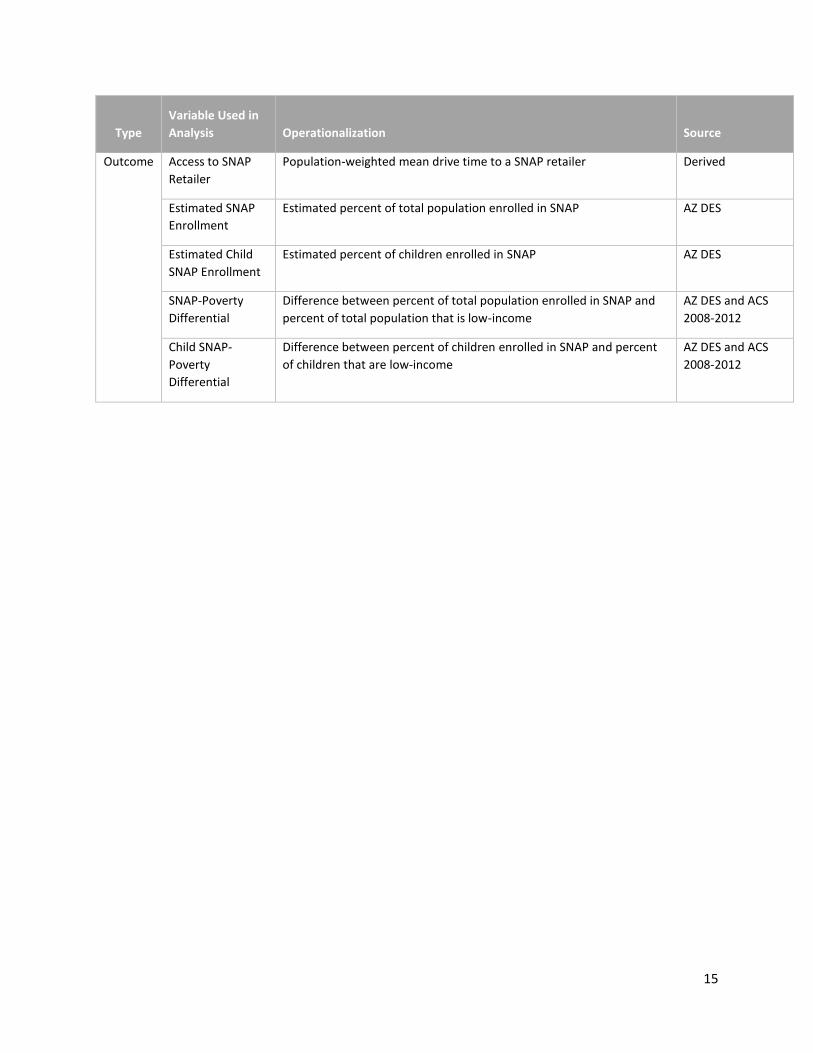
Type
Variable Used in
Analysis Operationalization Source
Outcome Access to SNAP
Retailer
Population-weighted mean drive time to a SNAP retailer Derived
Estimated SNAP
Enrollment
Estimated percent of total population enrolled in SNAP AZ DES
Estimated Child
SNAP Enrollment
Estimated percent of children enrolled in SNAP AZ DES
SNAP-Poverty
Differential
Difference between percent of total population enrolled in SNAP and
percent of total population that is low-income
AZ DES and ACS
2008-2012
Child SNAP-
Poverty
Differential
Difference between percent of children enrolled in SNAP and percent
of children that are low-income
AZ DES and ACS
2008-2012

16
Figure 1. Human Capital Factor

17
Figure 2. Population-Weighted Mean Drive Time to a SNAP retailer

18
Figure 3. Estimated Percent of Children Enrolled in SNAP

19
Figure 4.SNAP-Poverty Differential for Children (0-17)

20
Table 3. Cascade Analysis Results: Y1, Human Capital
Criterion Variable Prior Criterion Variables Predictor Variables Effect size F-ratio DF p
Human Capital Population Density -0.05 2.56 (1,383) 0.11
Slow Life History -0.03 .80 (1,383) 0.37
Median Age 0.10* 9.76 (1,383) 0.002
Work Engagement 0.19* 32.73 (1,383) <0.0001
Economic Sector 0.18* 9.88 (3,383) <0.0001
Primary 0.16* 22.10 (1,383) <0.0001
Secondary 0.09* 7.52 (1,383) 0.006
Tertiary 0.00 .01 (1,383) 0.92
Housing Health 0.09* 7.27 (1,383) 0.007
Income Equality 0.13* 16.42 (1,383) <0.0001
Migration 0.01 .19 (1,383) 0.66
Ethnicity 0.39* 45.96 (3,383) <0.0001
White 0.14* 18.54 (1,383) <0.0001
Hispanic/Latino -0.26* 62.11 (1,383) <0.0001
Other -0.25* 57.24 (1,383) <0.0001
Linguistic Isolation -0.42* 165.30 (1,383) <0.0001
Resource Access 0.38* 132.68 (1,383) <0.0001 Note: N=399. Where numerator df=1, the effect size is the semipartial correlation (sR); where numerator df>1, the effect size
is the multiple correlation (R), or, for the overall model, the eta/trace correlation (E).
*p<.05
Figure 5. Cascade Analysis Direct Effects: Y1, Human Capital

21
Table 4. Cascade Analysis Results: Y2, SNAP Drive Time
Criterion Variable Prior Criterion Variables Predictor Variables Effect size F-Ratio DF p
SNAP Drive Time Human Capital -0.24* 43.07 (1,382) <0.0001
Population Density -0.21* 31.37 (1,382) <0.0001
Slow Life History 0.03 0.66 (1,382) 0.42
Median Age 0.04 1.00 (1,382) 0.32
Work Engagement -0.09* 6.33 (1,382) 0.01
Economic Sector 0.20* 10.19 (3,382) <0.0001
Primary 0.01 0.08 (1,382) 0.78
Secondary -0.14* 14.49 (1,382) 0.0002
Tertiary -0.15* 15.99 (1,382) <0.0001
Housing Health -0.03 0.64 (1,382) 0.42
Income Equality 0.00 0.02 (1,382) 0.90
Migration -0.04 1.05 (1,382) 0.31
Ethnicity 0.13* 3.90 (3,382) 0.009
White 0.04 1.50 (1,382) 0.22
Hispanic/Latino -0.09* 5.86 (1,382) 0.02
Other -0.08* 4.36 (1,382) 0.04
Linguistic Isolation -0.21* 33.94 (1,382) <0.0001
Resource Access -0.52* 200.68 (1,382) <0.0001 Note: N=399. Where numerator df=1, the effect size is the semipartial correlation (sR); where numerator df>1, the effect size
is the multiple correlation (R), or, for the overall model, the eta/trace correlation (E).
*p<.05
Figure 6. Cascade Analysis Direct Effects: Y2, SNAP Drive Time

22
Table 5. Cascade Analysis Results: Y3, Child SNAP Enrollment
Criterion Variables Prior Criterion Variables Predictor Variables Effect Size F-Ratio DF p
Child SNAP Enrollment SNAP Drive Time -0.04 1.73 (1, 381) 0.19
Human Capital -0.53* 251.67 (1,381) <0.0001
Population Density 0.41* 147.65 (1, 381) <0.0001
Slow Life History -0.01 0.15 (1, 381) 0.70
Median Age 0.09* 6.42 (1, 381) 0.01
Work Engagement -0.08* 5.59 (1, 381) 0.02
Economic Sector 0.25* 17.83 (3, 381) <0.0001
Primary 0.20* 33.79 (1, 381) <0.0001
Secondary 0.10* 9.32 (1, 381) 0.002
Tertiary 0.11* 10.38 (1, 381) 0.001
Housing Health 0.04 1.59 (1, 381) 0.21
Income Equality -0.04 1.43 (1, 381) 0.23
Migration -0.04 1.44 (1, 381) 0.23
Ethnicity 0.12* 4.06 (3, 381) 0.007
White 0.02 0.40 (1, 381) 0.53
Hispanic/Latino 0.02 0.26 (1, 381) 0.61
Other -0.11* 11.52 (1, 381) 0.0008
Linguistic Isolation 0.13* 14.44 (1, 381) 0.0002
Resource Access -0.08* 5.59 (1, 381) 0.02 Note: N=399. Where numerator df=1, the effect size is the semipartial correlation (sR); where numerator df>1, the effect size
is the multiple correlation (R), or, for the overall model, the eta/trace correlation (E).
*p<.05
Figure 7. Cascade Analysis Direct Effects: Y3 Child SNAP Enrollment

23
Table 6. Cascade Analysis Results: Y4, Relative Child SNAP Enrollment
Criterion Variables Prior Criterion Variables Predictor Variables Effect Size F-Ratio DF p
Relative Child SNAP Enrollment Child SNAP Enrollment 0.67* 955.75 (1, 380) <0.0001
SNAP Drive Time -0.18* 69.64 (1, 380) <0.0001
Human Capital 0.46* 444.74 (1, 380) <0.0001
Population Density 0.03 2.34 (1, 380) 0.13
Slow Life History 0.07* 9.59 (1, 380) 0.002
Median Age 0.12* 28.76 (1, 380) <0.0001
Work Engagement 0.16* 54.82 (1, 380) <0.0001
Economic Sector 0.18* 22.72 (3, 380) <0.0001
Primary -0.18* 68.01 (1, 380) <0.0001
Secondary 0.01 0.14 (1, 380) 0.71
Tertiary 0.00 0.00 (1, 380) 0.90
Housing Health 0.04 2.84 (1, 380) 0.09
Income Equality 0.14* 41.57 (1, 380) <0.0001
Migration -0.13* 38.43 (1, 380) <0.0001
Ethnicity 0.12* 10.88 (3, 380) <0.0001
White -0.08* 14.33 (1, 380) 0.0002
Hispanic/Latino -0.05* 4.68 (1, 380) 0.03
Other 0.08* 13.62 (1, 380) 0.0003
Linguistic Isolation -0.07* 9.27 (1, 380) 0.002
Resource Access 0.01 0.23 (1, 380) 0.63 Note: N=399. Where numerator df=1, the effect size is the semipartial correlation (sR); where numerator df>1, the effect size
is the multiple correlation (R), or, for the overall model, the eta/trace correlation (E).
*p<.05
Figure 8. Cascade Analysis Direct Effects: Y4, Relative Child SNAP Enrollment

24
Figure 9.Total Cascade Analysis Effects

25
Figure 10. Arizona Rural Clusters

26
Table 7. Cluster Descriptions
CLUSTER KEY CHARACTERISTICS
Ag, Mining, Forestry Highest Primary-sector Employment, Low Population Density, Lowest Tertiary-sector Employment
Border City High Population Density, Highest Linguistic Isolation, Highest Migration, Highest Hispanic Population, Low Housing Capital
Border Periphery High Migration, High Hispanic population, High Primary-sector Employment, High Linguistic Isolation
Mixed Migrant High Migration, Most Ethnically Diverse, High Primary-sector Employment, High Secondary-sector Employment
Suburb/Historically Mormon Highest Resource Access, Highest Income Equality, Highest Work Engagement, Lowest Primary-sector Employment
Retirees Highest Median Age, Low Work Engagement, Slowest Life History, Highest White Population, High Human Capital
Scenic High Median Age, Highest Housing Capital, High Work Engagement, High Secondary-sector Employment, High White Population
Tribal Low Median Age, Fast Life History, Low Income Equality, Low Migration, Highest non-white and non-Hispanic population
Table 8. Outcome Variables by Cluster
HUMAN CAPITAL SNAP DRIVE
TIME SNAP ENROLLMENT
(CHILD) RELATIVE SNAP
ENROLLMENT (CHILD) Cluster N MEAN SD MEAN SD MEAN SD MEAN SD
Tribal 45 0.179 0.102 0.275 0.170 0.580 0.199 -0.196 0.216
Mixed Migrant 39 0.358 0.098 0.127 0.182 0.427 0.165 -0.194 0.243
Border Periphery 16 0.300 0.078 0.055 0.072 0.583 0.212 -0.130 0.224
Ag/Mining/Forestry 28 0.424 0.081 0.222 0.170 0.380 0.198 -0.124 0.251
Retiree 60 0.498 0.142 0.126 0.146 0.425 0.353 -0.086 0.367
Scenic 104 0.493 0.139 0.139 0.153 0.357 0.356 -0.066 0.314
Mormon/Suburb 100 0.489 0.107 0.057 0.096 0.331 0.235 -0.060 0.218
Border City 7 0.220 0.062 0.007 0.011 1.207 0.622 0.396 0.671
27
7 REFERENCES
Abarca, J., & Ramachandran, S. (2005). Using community indicators to assess nutrition in Arizona-Mexico border communities. Preventing Chronic Disease, 2(1), A06.
Alwitt, L. F., & Donley, T. D. (1997). Retail stores in poor urban neighborhoods. The Journal of Consumer Affairs, 31(1), 139-164.
Bader, M. D. M., Purciel, M., Yousefzadeh, P., & Neckerman, K. M. (2010). Disparities in neighborhood food environments: implications of measurement strategies. Economic Geography, 86(4), 409–30.
Bartfeld, J., Dunifon, R., & Chandran, R. (2005). State-Level predictors of food insecurity and hunger among households with children.
Bertrand, L., Thérien, F., & Cloutier, M. (2008). Measuring and mapping disparities in access to fresh fruits and vegetables in Montréal. Canadian Journal of Public Health / Revue Canadienne De Sante'e Publique, 99(1), 6-11.
Boehmer, T. K., Lovegreen, S. L., Haire-Joshu, D., & Brownson, R. C. (2006). What constitutes an obesogenic environment in rural communities? American Journal of Health Promotion, 20(6), 411–21.
Burns, C. M., Gibbon, P., Boak, R., Baudinette, S., & Dunbar, J. A. (2004). Food cost and availability in a rural setting in Australia. Rural and Remote Health, 4(311).
Cabeza de Baca, T., Figueredo, A.J., & Ellis, B.J. (2012). An evolutionary analysis of variation in parental effort: Determinants and assessment. Parenting: Science and Practice, 12, 94-104).
Cummins, S., & Macintyre, S. (2002). “Food deserts”--evidence and assumption in health policy making. BMJ (Clinical Research Ed.), 325(7361), 436–8.
Eicher, C. L., & Brewer, C. A. (2001). Dasymetric Mapping and Areal Interpolation: Implementation and Evaluation. Cartography and Geographic Information Science, 28(2), 125–138.
Demetriou, A., Christou, C., Spanoudis, G., Platsidou, M., Fischer, K. W., & Dawson, T. L. (2002). The development of mental processing: Efficiency, working memory, and thinking. Monographs – Society for Research in Child Development, 67(268), ALL.
Figueredo, A. J., & Gorsuch, R. L. (2007). Assortative mating in the jewel wasp. 2: Sequential canonical analysis as an exploratory form of path analysis. Journal of the Arizona-Nevada Academy of Science, 39(2), 59-64.
Finegold, K., Pindus, N., Levy, D., Tannehill, T. & Hillabrant, W. (2009). Tribal Food Assistance: A Comparison of the Food Distribution Program on Indian Reservations (FDPIR) and the Supplemental Nutrition Assistance Program (SNAP). Washington, D.C: The Urban Institute.
Genser, J. L. (2009). Diet Quality of Americans by SNAP (Food Stamp) Participation Status. Journal of Nutrition Education and Behavior, 41(4S), 2157.
Gordon-Larsen, P., Nelson, M. C., Page, P., & Popkin, B. (2006). Inequality in the built environment underlies key health disparities in physical activity and obesity. Pediatrics, 117(2), 417–424.
Guy, C. M. (1991). Urban and rural contrasts in food prices and availability—a case study in wales. Journal of Rural Studies, 7(3), 311–325.
Han, E., Powell, L. M., & Isgor, Z. (2012). Supplemental nutrition assistance program and body weight outcomes: the role of economic contextual factors. Social Science & Medicine (1982), 74(12), 1874–81.
Holt, J. B., Lo, C. P., & Hodler, T. W. (2004). Dasymetric estimation of population density and areal interpolation of census data. Cartography and Geographic Information Science, 31(2), 103-121.
Hosler, A. S., Varadarajulu, D., Ronsani, A. E., Fredrick, B. L., & Fisher, B. D. (2006). Low-fat milk and high-fiber bread availability in food stores in urban and rural communities. Journal of Public Health Management and Practice : JPHMP, 12(6), 556–62.
Jackson, R. J. (2003). The impact of the built environment on health: an emerging field. American Journal of Public Health, 93(9), 1382–4.
Kaufman, P. R. (1999). Rural Poor Have Less Access to Supermarkets, Large Grocery Stores. Rural Development Perspectives, 13(3), 19–26.
Lacombe, D. J., Michieka, N. M., & Gebremedhin, T. (2012). A Bayesian Spatial Econometric Analysis of SNAP Participation Rates in Appalachia. The Journal of Regional Analysis & Policy, 42(3), 198–209.

28
Larsen, K., & Gilliland, J. (2008). Mapping the evolution of 'food deserts' in a Canadian city: Supermarket accessibility in London, Ontario, 1961-2005. International Journal of Health Geographics, 7(1), 16-16.
Larson, N. I., Story, M. T., & Nelson, M. C. (2009). Neighborhood environments: disparities in access to healthy foods in the U.S. American Journal of Preventive Medicine, 36(1), 74–81.
Lefttin, J., Eslami, E., & Strayer, M. (2011). Trends in Supplemental Nutrition Assistance Program participation rates: Fiscal year 2002 to fiscal year 2009 (pp. 1–65). Washington, D.C.
Leung, C. W., Blumenthal, S. J., Hoffnagle, E. E., Jensen, H. H., Foerster, S. B., Nestle, M., … Willett, W. C. (2013). Associations of food stamp participation with dietary quality and obesity in children. Pediatrics, 131(3), 463–72. doi:10.1542/peds.2012-0889
Leung, C. W., & Villamor, E. (2011). Is participation in food and income assistance programmes associated with obesity in California adults? Results from a state-wide survey. Public Health Nutrition, 14(4), 645–52. doi:10.1017/S1368980010002090
Li, C., Balluz, L. S., Ford, E. S., Okoro, C. a, Zhao, G., & Pierannunzi, C. (2012). A comparison of prevalence estimates for selected health indicators and chronic diseases or conditions from the Behavioral Risk Factor Surveillance System, the National Health Interview Survey, and the National Health and Nutrition Examination Survey, 2007-2008. Preventive Medicine, 54(6), 381–7.
Liese, A. D., Weis, K. E., Pluto, D., Smith, E., & Lawson, A. (2007). Food store types, availability, and cost of foods in a rural environment. Journal of the American Dietetic Association, 107(11), 1916–23.
Lois, B., Morton, W., & Blanchard, T. C. (2007). Starved for Access: Life in Rural America’s Food Deserts, 1(4), 1–10. Lwin, K. K., & Murayama, Y. (2010). Development of GIS Tool for Dasymetric Mapping. International Journal of
Geoinformatics, 6(1), 11–18. Lytle, L. A. (2009). Measuring the food environment: state of the science. American Journal of Preventive Medicine,
36(4 Suppl), S134–44. Macintyre, S., Ellaway, A., & Cummins, S. (2002). Place effects on health: how can we conceptualise, operationalise
and measure them? Social Science & Medicine, 55(1), 125–139. McEntee, J., & Agyeman, J. (2010). Towards the development of a GIS method for identifying rural food deserts:
Geographic access in vermont, USA. Applied Geography, 30(1), 165-176. McKinnon, R., Reedy, J., Morrissette, M. a, Lytle, L. a, & Yaroch, A. L. (2009). Measures of the food environment: a
compilation of the literature, 1990-2007. American Journal of Preventive Medicine, 36(4 Suppl), S124–33. Mennis, J. (2003). Generating Surface Models of Population Using Dasymetric Mapping*. The Professional
Geographer, 55(1), 31–42. Nelson, D. E., Powell-Griner, E., Town, M., & Kovar, M. G. (2003). A comparison of national estimates from the
National Health Interview Survey and the Behavioral Risk Factor Surveillance System. American Journal of Public Health, 93(8), 1335–41.
Oliveira, V. (2014). Food Assistance Landscape: FY 2013 Annual Report, EIB-120. U.S. Department of Agriculture, Economic Research Services.
Openshaw, S. (1984). Ecological fallacies and the analysis of areal census data. Environment & Planning A, 16(1), 17 Pearce, J., Witten, K., & Bartie, P. (2006). Neighbourhoods and health: A GIS approach to measuring community
resource accessibility. Journal of Epidemiology and Community Health (1979-), 60(5), 389-395. Pierannunzi, C., Hu, S. S., & Balluz, L. (2013). A systematic review of publications assessing reliability and validity of
the Behavioral Risk Factor Surveillance System (BRFSS), 2004-2011. BMC Medical Research Methodology, 13(49).
Powell, L. M., Slater, S., Mirtcheva, D., Bao, Y., & Chaloupka, F. J. (2007). Food store availability and neighborhood characteristics in the United States. Preventive Medicine, 44(3), 189–95.
Rose, D., & Richards, R. (2004). Food store access and household fruit and vegetable use among participants in the US Food Stamp Program. Public Health Nutrition, 7(8), 1081–8.
Sallis, J. E., & Glanz, K. (2006). The role of built environments in physical activity, eating, and obesity in childhood. The Future of Children, 16(1), 89–108.
Scholz, J., & Herrmann, S. (2010). Rural regions in Europe. A new typology showing diversity of European rural regions. European Union FP 7 RUFUS (Rural Future Networks Project).
Sharkey, J. R. (2009). Measuring potential access to food stores and food-service places in rural areas in the U.S. American Journal of Preventive Medicine, 36(4 Suppl), S151–5.

29
Sharkey, J. R., & Horel, S. (2008). Neighborhood socioeconomic deprivation and minority composition are associated with better potential spatial access to the ground-truthed food environment in a large rural area. The Journal of Nutrition, 138(3), 620–7. Retrieved from http://www.ncbi.nlm.nih.gov/pubmed/18287376
Shaw, H. J. (2014). Food deserts: Towards the development of a classification. Geografiska Annaler. Series B, Human Geography, 88(2), 231–247.
Simen-Kapeu, A., Kuhle, S., & Veugelers, P. J. (2010). Geographic Differences in Childhood Overweight, Physical Activity, Nutrition and Neighbourhood Facilities: Implications for Prevention. Canadian Journal of Public Health, 101(2), ALL.
Simmons, S., Alexander, J. L., Ewing, H., & Whetzel, S. (2012). SNAP Participation in Preschool-Aged Children and Prevalence of Overweight. Journal of School Health, 82(12), 548–553.
Srinivasan, S., O’Fallon, L. R., & Dearry, A. (2003). Creating healthy communities, healthy homes, healthy people: initiating a research agenda on the built environment and public health. American Journal of Public Health, 93(9), 1446–50.
USDA (2007). Arizona rural definitions maps. Retrieved from http://www.ers.usda.gov/data-products/rural-definitions.aspx
Vartanian, T. P., & Houser, L. (2012). The effects of childhood SNAP use and neighborhood conditions on adult body mass index. Demography, 49(3), 1127–54. doi:10.1007/s13524-012-0115-y
Ver Ploeg, M., Breneman, V., Farrigan, T., Hamrick, K., Hopkins, D., Kaufman, P., Kim, S. (2009). Access to Affordable and Nutritious Food : Measuring and Understanding Food Deserts and Their Consequences- Report to Congress (pp. 1–150). U.S. Department of Agriculture, Economic Research Services.
Ver Ploeg, M., Dutko, P., & Breneman, V. (2015). Measuring food access and food deserts for policy purposes. Applied Economic Perspectives and Policy, 37(2), 205-225
Walker, R. E., Keane, C. R., & Burke, J. G. (2010). Disparities and access to healthy food in the United States: A review of food deserts literature. Health & Place, 16(5), 876–84.
Walsh, M., Katz, M., Sechrest, L. (2002). Unpacking cultural factors in adaptation to Type II diabetes mellitus. Medical Care, 40(1 Supp), 129-139.
Walsh, M., Smith, R., Morales, A. & Sechrest, L. (2000). Ecocultural Research: A Mental Health Researcher’s Guide to the Study of Race, Ethnicity, and Culture. Human Services Research Institute: Cambridge, MA.
Wang, M. C., Gonzalez, A. A., Ritchie, L. D., & Winkleby, M. A. (2006). The neighborhood food environment : sources of historical data on retail food stores. International Journal of Behavioral Nutrition and Physical Activity, 3(15), 1–5


