
Universita degli Studi di Milano
Facolta di Scienze Matematiche, Fisiche e Naturali
Laurea Triennale in Fisica
Plateau Dynamics of aLubricated Friction Model
Relatore: Dott. Nicola Manini
Correlatore: Prof. Giuseppe Santoro
Marco Cesaratto
Matricola n◦ 656734
A.A. 2005/2006
Codice PACS: 68.35.Af

2

Plateau Dynamics
of a Lubricated
Friction Model
Marco Cesaratto
Dipartimento di Fisica, Universita di Milano,
Via Celoria 16, 20133 Milano, Italia
Abstract
In this work we study a generalized Frenkel-Kontorova friction model
with two sliding periodic substrate potentials acting on a harmonic chain
representing the lubricant. We compare the dynamics of the lubricant
applying different boundary conditions: periodic, representing an infinite
chain, and open, simulating a lubricant of finite size, such as a hydrocar-
bon chain molecule would be. In particular, we investigate the velocity
quantization phenomena recently found in the motion of the infinite-size
lubricant chain: this quantization is due to one slider rigidly dragging the
kinks that the chain forms with the other slider. We extend these results
to the finite-size case, that (i) like the infinite-size chain permits the devel-
opment of robust velocity plateaus as a function of the lubricant stiffness,
and (ii) allows an overall chain-length re-adjustment which spontaneously
promotes single-particle periodic oscillations. These periodic oscillations
take the place of the quasi-periodic motion produced by generally incom-
mensurate periods of the sliders and the lubricant in the infinite-size model.
We also report the hysteretic behavior, analogous to that of static friction,
found as the dynamics of the chain leaves the plateau regime under the
action of an additional constant external driving force.
Advisor: Dr. Nicola Manini
Co-Advisor: Prof. Giuseppe Santoro

Contents
1 Introduction 5
2 The Model 6
3 Numerical Method 8
3.1 Periodic boundary conditions . . . . . . . . . . . . . . . . . . . . 9
3.2 Open boundary conditions . . . . . . . . . . . . . . . . . . . . . . 10
3.3 Initial conditions . . . . . . . . . . . . . . . . . . . . . . . . . . . 10
4 The plateau dynamics 14
4.1 Infinite-size lubricant chains . . . . . . . . . . . . . . . . . . . . . 14
4.2 Finite-size lubricant chains . . . . . . . . . . . . . . . . . . . . . . 22
4.2.1 Size dependence of the CM velocity . . . . . . . . . . . . . 28
4.2.2 Boundary effects on the fluctuations . . . . . . . . . . . . 30
5 Hysteresis 33
6 Conclusions 35
Bibliography 37
4

1 Introduction
We study an atomic-scale friction model derived from the classical Frenkel-Kon-
torova (FK) model. The standard FK model describes the dynamics of a chain
of particles interacting via harmonic springs, and subjected to the action of an
external periodic potential. Recently, on the FK model and related systems,
Braun and Kivshar published an extensive review book [1]. One of the most
interesting features in the standard FK model is the Aubry transition. When the
ratio between the period of the external potential and that of the free chain is
commensurate, for any spring stiffness K the chain is “pinned” to the substrate,
and a finite driving force is needed in order to start sliding. In the irrational case,
otherwise, a critical value of K exist, KAubry, so that for K > KAubry the system
is “unpinned”: sliding begins under any nonzero applied force. For K < KAubry
the system remains “pinned”, as in the commensurate case [2].
Variations of the standard FK model including multiple chains have been
studied and look promising for the simulation of inter-facial slip. Other applica-
tions have been found in several fields, including dislocation dynamics, adsorbed
atomic layers, incommensurate phases in dielectrics, lattice defects, magnetic
chain and hydrogen-bonded chains [1]. In recent years, more possible applica-
tions appeared in the study of vortex matter [3], novel topological defects [4]
and high-Tc superconductors. Due to the current hype on nanotechnologies, the
FK model as also been employed to explain the basic principles of atomic-scale
engines [5].
In this work we analyze the velocity quantization phenomena recently found
in the classical motion of an idealized 1D model solid lubricant, consisting of a
harmonic infinite chain interposed between two periodic sliding potentials [6, 7].
Previous studies addressed the infinite-size thermodynamical limit, where fixed
commensurate and incommensurate length ratios are imposed. We extend this
study to a lubricant 1D “island” of finite size; we continue to find velocity plateaus
due to kink dynamics, like in the infinite-size chain. The novelty of finite-size is
that the plateau dynamics shows a strong tendency to periodic oscillations, thanks
to a self-directed chain-length re-adjustment. Finally, we report the hysteretic
behavior found in the dynamics of the infinite-length chain, under the action of
an additional external driving force.
5

Figure 1: A sketch of the model with the two periodic sliders (periods a+ and
a−) and the lubricant harmonic chain of rest nearest-neighbor length a0.
2 The Model
We represent two solids touching each other as periodic (sine or cosine) poten-
tials with periodicity equal to the substrate lattice constants (Fig. 1). The lu-
bricant is composed by a chain of particles joined by springs. We consider only
nearest-neighbor coupling and interaction terms up to second order (harmonic
approximation). Our model differs from the usual FK model, which is based on a
single periodic potential acting on a spring chain, in being based on two periodic
potentials, one of which is shifting.
The Lagrangian is
L = T − U , (1)
T and U being the kinetic and potential energies. The classical kinetic energy is
T =∑
i
1
2mx2
i , (2)
where m is the particle mass and xi is the velocity of particle i, at position xi.
The potential energy U consists of two parts:
U = Usub + Uspring . (3)
The first term characterizes the interaction of the lubricant chain with the two
external periodic potentials representing the solid substrates:
Usub({xi}) = −1
2
∑
i
[u+ cos (k+xi) + u− cos (k−xi)] . (4)
In Eq. (4)
k± =2π
a±(5)
6

are the wave vectors associated to the (generally different) periodicities of the two
substrate potentials, of amplitudes u±. The second term accounts for the energy
of the springs:
Uspring({xi}) =K
2
∑
i
(xi+1 − xi − a0)2 . (6)
a0 is the equilibrium length of the isolated harmonic spring, of restoring constant
K.
Consider driving the two layers to move at constant velocities v±. The time-
dependent potential acting on the particles is then
Usub({xi}, t) = −1
2
∑
i
{u+ cos [k+(xi − v+t)] + u− cos [k−(xi − v−t)]} . (7)
We introduce a phenomenological friction force to account for the energy
loss of the moving masses, −γ∑
i(xi − vw). The γ term is meant to account for
all dissipative losses to electronic and phononic degrees of freedom of the two
substrates. A term −γ(xi − v+) refers to the first substrate, and analogously
−γ(xi − v−) refers to the second one, whence it is natural to choose vw = v++v−
2.
Accordingly, the classical equations of motion are
mxi = −1
2{F+ sin[k+(xi − v+t)] + F− sin[k−(xi − v−t)]} +
+K(xi+1 + xi−1 − 2xi) − 2γ(xi − vw) , (8)
where F± = k±u± are the force amplitudes representing the sinusoidal corrugation
of the two sliders.
Henceforth, we choose the reference frame in which v+ = 0 and v− = vext
(so that vw = vext/2). The three different periodicities a± and a0 define two
independent ratios:
r± =a±
a0
. (9)
We assume, without loss of generality, r− > r+.
In view of limiting the dimensionality of the parameters space, we use equal
substrate forces F− = F+ = F . We take a+ as length unit, the mass m of
lubricant particles as mass unit and F as force unit. This choice defines a set of
“natural” units for all physical quantities, which are henceforth implicitly defined
in terms of these units, and expressed as dimensionless numbers. To obtain a
physical quantity in its explicit dimensional form, one should simply multiply its
numerical value by the corresponding natural units shown in Table 1.
7

Physical quantity Natural units
length a+
mass m
force F
energy a+ F
velocity v a1/2+ F 1/2 m−1/2
time a1/2+ F−1/2 m1/2
spring constant K a−1+ F
viscous friction γ a−1/2+ F 1/2 m1/2
Table 1: Natural units for several physical quantities in a system where length,
force and mass are measured in units of a+, F , and m respectively.
This two-sliders model has already been introduced by Vanossi et al. [8, 9].
They considered (r+, r−) = (r, r2), and centered their works on the study of the
force needed in order to start sliding, finding that for both a commensurate and a
quadratic irrational r a finite force is required, while a cubic irrational r presents
an Aubry transition. In that version of the model, however, the chain was pulled
by a constant force between static substrates. A model similar to the one studied
here was treated in Ref. [10]: sliding of the top substrate was achieved through
the application of a constant driving, via an additional spring. We instead choose
to move one of the layers at a constant speed vext. Previous work [6, 7] on this
same model found robust, universal and exactly quantized asymmetric velocity
plateaus in the dynamics of an infinite-size chain.
3 Numerical Method
To solve the differential equations of motion (8) we use a standard adaptive
fourth-order Runge-Kutta algorithm [11]. The model described in Sect. 2 can be
addressed with as a target a chain of infinite length (as done in Ref. [6, 7]) or a
finite-size chain. In the first case, in practice a finite number N of particles must
be considered: finite-size effects are minimized by applying periodic boundary
conditions (PBC) and considering appropriate size scaling. In the second case,
instead, open boundary conditions (OBC) must be used. Notice that in the
equations of motion (8) no mention is made of the inter-particle equilibrium
length a0, which is only introduced in the dynamics by the boundary conditions.
8

3.1 Periodic boundary conditions
To represent the infinite-size model, PBC are taken: it is thus possible to enforce
a fixed-density condition for the chain, with a coverage r+ of chain atoms on
the denser substrate. In this case a0 does not enter explicitly the equations of
motion (8) and appears only via the boundary condition xN+1 = x1 + Na0.
PBC are straightforward for rational r±. In the irrational case, PBC may
be realized by approximating a−/a+ and r+ = a+/a0 with suitable rational num-
bers N+/N− and N/N+, obtained, e.g., by means of a continued fraction ex-
pansion. For example, convenient rational approximants of the Golden Mean
(GM) φ = (√
5 + 1)/2 (solution of φ2 = φ + 1) are provided by the Fibonacci
sequence Fn+1 = Fn + Fn−1, F0 = F1 = 1, so that taking a+/a0 = Fn+1/Fn and
a−/a+ = Fn/Fn−1 leads to a finite system with N = Fn+1 particles, occupying a
ring of length Na0 with PBC, subject to the two substrate potentials with, respec-
tively, Fn (+) and Fn−1 (−) minima. This method introduces a finite-size error
which is distributed uniformly through the system. Approaching a problem in
which incommensuration is one of the key features by employing rational approx-
imation might appear puzzling. However, by scaling the approximate sequence,
one realizes perfect PBC and produces a sequence of rational approximants con-
verging correctly to the appropriate irrational. Unfortunately, the method of the
continued fraction works efficiently only in few cases.
Alternatively, we rather choose to use the machine precision values of the
length ratios r+ and r− using a more literal implementation of PBC for Uspring.
Problem is that, in general, for arbitrary N , the first and last mass generally find
themselves in a shifted position relative to Usub with respect to their periodic
images. The PBC would be perfectly implemented only if the “(N + 1)-th” mass
was in the same static situation as the first one. Take the position of x1 at the
origin of the coordinate and let it correspond, say, to a minimum in the potential:
the “(N + 1)-th” mass is L = Na0 away from the origin. Its phase shifts relative
to the two oscillations in Usub potential minimum are
δ± = 2π
∣
∣
∣
∣
N± − N
r±
∣
∣
∣
∣
, (10)
with N± = [N/r±], where [ ] indicates rounding to the nearest integer. For PBC
to be implemented perfectly these two quantities should vanish exactly. This can
be done only with rational values of the length ratios r+ and r−. When simulating
irrational values we minimize the total shift error δtot = |δ−|+ |δ+| with respect to
the number of particles N : this error can be made arbitrarily small by choosing
9

suitably large integers N , N±. The finite-size error introduced by this method
remains concentrated where the boundary condition applies. We have checked
that the effects of this phase error become extremely small, and hardly visible,
as long as δtot < 0.1.
3.2 Open boundary conditions
In the case of a finite open-boundary chain (representing for example a hydro-
carbon chain, or a graphite flake interposed between two sliding crystal faces), a0
enters explicitly the equations of motion (8) of the first (i = 1) and last (i = N)
particle, where the restoring force terms are K(x2−x1−a0) and K(xN−1−xN +a0),
respectively.
The main difference between OBC and PBC is that, while in PBC the chain
length, and thus the length ratios r±, are fixed, in OBC the chain can stretch
or shorten with respect to its equilibrium size. We find that the chain does so
spontaneously: during sliding, the chain length gradually drifts toward a natural
attractor value and oscillates around it (see Fig. 2). This final stable length
defines a new effective inter-particle length and a corresponding length ratio
aeff0 =
L
N − 1, reff
+ =a+
aeff0
, (11)
where L = 〈xN − x1〉 is the average chain length after the initial transient. The
effective length ratio reff+ plays a central role in the understanding of the velocity
plateaus of the finite-size lubrication model.
3.3 Initial conditions
In our computations we integrate the equations of motion (8) starting from fully
relaxed springs, i.e. we impose a distance a0 between neighbor particles: xi = (i−1)a0. We also assume that the chain is initially shifting with speed vext/2. After
an initial transient, the system reaches its dynamical stationary state, at least so
long as γ is not exactly zero. As a consequence, the center-of-mass (CM) velocity
stabilizes, but it continues to execute small-amplitude oscillations. Figure 3 shows
the CM velocity as a function of time for open chains of different size, in the
stationary regime after the initial transient. First, observe that these oscillations
are perfectly periodic. Next, note that the amplitude of these oscillations is
clearly size-dependent: it decreases approximately as 1/N . In particular, detailed
10

-1.5-1
-0.50
0.51
1.5
v cm /
v ext
0.660.68
0.70.720.740.760.78
0 5000 10000 15000 20000t
0.660.68
0.70.720.740.760.78
(xN-x
1)/(N-
1)
N = 100
N = 200
N = 100
a0eff
effa0
Figure 2: CM velocity (upper panel) and mean inter-particle distance (central
and bottom panels) as a function of time, for an open chain of length N = 100
or 200, and (r+, r−) = (√
103100
+ 26100
,√
101) ' (1.2749, 10.050), K = 4, vext = 0.01,
γ = 0.1. With this choice of parameters, during the initial transient the chain
length gradually decreases. The CM velocity is chaotic while length relaxation
takes place, but eventually it becomes periodic when the stationary state is
reached. The final aeff0 and average velocity vcm reached is the same, irrespec-
tive of N : aeff0 = 0.664, vcm/vext = 0.337 (deviations from the calculated value of
aeff0 are explained in Sect. 4.2.2 below). Note however that the transient duration
is size-dependent: it is approximately twice longer for N = 200 than for N = 100.
11

1000 2000 3000 4000t - 100000
-0.5
0
0.5
1
1.5
2
2.5
3
3.5
4
v cm /
v ext
N=100
N=200
N=500
N=1000
Figure 3: CM velocity as a function of time, for different sizes of the chain:
N = 100, 200, 500 and 1000 (bottom to top) in the stationary regime past the
initial transient. The velocity performs periodic oscillations, whose amplitude ap-
proximately decreases as 1/N . Note the presence of larger-amplitude oscillation,
due to boundary effects (see Fig. 15 below). Velocity is shifted upward by 0, 2,
3, 3.6 respectively, for better clarity. Same parameters as in Fig. 2.
12

0 5000 10000t
0.7
0.8
0.9
1
1.1
1.2
1.3
1.4
1.5
(xN-x
1)/(N-
1)xi = (i-1) a0
xi = (i-1) 2a0
Figure 4: Mean inter-particle distance as a function of time, for two different
initial conditions: xi = (i − 1)a0 (relaxed springs, solid curve) and xi = (i −1)2a0 (stretched springs, dashed curve). In the second case the chain is initially
twice longer, but the mean interparticle length reaches the same attractor value
aeff0 = 0.664, approximately in the same time. Here N = 100 and the dynamical
parameters are the same as in Fig. 2.
analysis of the motion of the single particles shows that the larger-amplitude
spikes in the dynamics of finite-size chains are boundary effects, caused by the
kinks (see Sect. 4 below) forming at one end and going out from the chain at the
other end. These effects are of course not present when PBC are applied, or in
the infinite-size limit.
OBC allow length relaxation to take place during the initial transient. Fig-
ure 2 shows the time-evolution of the mean inter-particle distance xN−x1
N−1, for two
different sizes of the chain: N = 100 and N = 200. The relaxation that takes
place during this transient is not driven by the viscous term introduced in Eq. (8):
we checked that the length-relaxation (even its duration) is very weakly influenced
by γ, for wide ranges of this parameter in the underdamped regime. By changing
13

the initial conditions, we checked that the “dynamical stationary state” realized
after the transient is independent of the initial state considered (see for example
Fig. 4). As we are interested in the stationary state of the system, we do not
include the initial transient in all averages.
4 The plateau dynamics
We study here the driven two-substrate model introduced in Sect. 2, first in the
infinite-size case and then for chains of finite length. We focus our attention on
the exact velocity quantization phenomena reported in Ref. [6, 7]: we find that
the ratio vcm/vext of the chain center-of-mass (CM) velocity to the externally im-
posed relative velocity of the sliders stays pinned to exact plateau values for wide
ranges of parameters, such as slider corrugation amplitudes, external velocity,
chain stiffness, and dissipation, and is strictly determined by the commensura-
bility ratios alone. This phenomenon is explained by one slider rigidly dragging
the kinks (topological solitons) that the chain forms with the other slider. In
particular, OBC simulations show that the PBC used in Ref. [6, 7] are not cru-
cial to the plateau quantization, which occurs even for a lubricant of finite size
and not particularly large N , such as a hydrocarbon chain molecule would be. In
addition, OBC chains approach spontaneously such values of L as to implement
perfectly periodic orbits, even for incommensurate r+ and r− which would lead
to chaotic motion in PBC.
4.1 Infinite-size lubricant chains
We illustrate here the results obtained from simulations relative to the infinite-
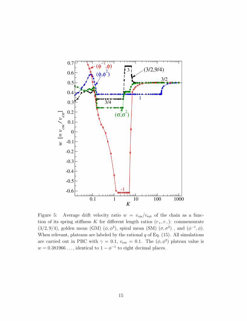
size model, i.e. with the boundary conditions described in Sect. 3.1. Figure 5
shows the time-averaged CM velocity vcm as a function of the chain stiffness K
for four representative (r+, r−) values, three with r+ > 1 and r− = r2+, and one
with r+ < 1. The velocity ratio w = vcm/vext is generally a complicated function
of K, with flat plateaus and regimes of continuous evolution, in a way which is
qualitatively similar for different cases. The main surprise is that all plateaus
show perfectly flat w that are constant (quantized) to all figures of numerical
accuracy, the precise value strikingly independent not only of K, but also of γ,
vext, and even of F−/F+.
To explore the origin of the universality of w, we analyze the dynamics for
14
-0.6
-0.5
-0.4
-0.3
-0.2
-0.1
0
0.1
0.2
0.3
0.4
0.5
0.6
0.7w
[= v
cm /
v ext]
0.1 1 10 100 1000K
(φ,φ2)(3/2,9/4)
13/4
3
3/2
-1
(φ−1,φ)
(σ,σ2)
Figure 5: Average drift velocity ratio w = vcm/vext of the chain as a func-
tion of its spring stiffness K for different length ratios (r+, r−): commensurate
(3/2, 9/4), golden mean (GM) (φ, φ2), spiral mean (SM) (σ, σ2) , and (φ−1, φ).
When relevant, plateaus are labeled by the rational q of Eq. (15). All simulations
are carried out in PBC with γ = 0.1, vext = 0.1. The (φ, φ2) plateau value is
w = 0.381966 . . . , identical to 1 − φ−1 to eight decimal places.
15

1.2 1.4 1.6 1.8 2r+
0.1
0.2
0.3
0.4
0.5
wpl
atea
u
1 - (r+)-1
r- = (r+)2
Figure 6: The main plateau velocity w as a function of r+, for (r+, r−) = (r+, r2+).
To produce an irrational value of r±, we set r+ =√
101100
+ i100
, with i = 0, 1, 2..., 99,
so that 1 < r+ < 2. All calculations were carried out for vext = 0.1, γ = 0.1.
The value of N for each calculation was set to the lowest N such that δtot < 0.1:
the values ranged from N ∼ 100 to N ∼ 5000. Each dot represents a value of
r+ for which at least 3 different values of the spring constant K yield the same
plateau value of vcm within 10−3. The numerical plateau velocity ratios (dots) are
compared to Eq. (12). Note that no plateaus are found for r+ close to unity: the
reason is that r− = r2+ ' 1 when r+ ' 1, so the periodicities of the two substrate
are too similar and the kink mechanism does not apply.
16

1 2 3 4r+
-0.5
-0.25
0
0.25
0.5
0.75
wpl
atea
u
1 - (r+)-1
φ
17/13-(10)-1/21031/1000
π/2
3/2
σ
φ−1
16/7
2+51/2
π
Figure 7: The main plateau velocity w as a function of r+, in the range 0.5 < r+ <
4.5. Labels refer to r+ values. Most calculations are carried out with r− = r2+,
except (r+ = φ−1, r− = φ), (r+ = 1713
− 1√10
, r− = 7), (r+ = 10311000
, r− =√
101),
and (r+ = π, r− =√
101 + 10). Other parameters are vext = 0.1, γ = 0.1. Note
that the plateau velocity follows Eq. (12) even for r+ < 1, leading to negative
values.
17

a large number of values of (r+, r−), commensurate and incommensurate, and
observe that:
• at least one velocity plateau as a function of K occurs for any (r+, r−),
unless r+ and r− are both very close to unity;
• additional narrower secondary plateaus often arise for stiffer lubricant, i.e.
for larger K (see Fig. 5);
• the “natural” symmetric limit w = 1/2 is always approached for large K;
• the velocity ratio w of the first plateau found for increasing K satisfies
w = 1 − r−1+ (12)
for a large range of (r+, r−).
This last observation is supported by the data of Fig. 6, where we report a
systematic study of the main-plateau velocity w as a function r+ in the range
1 < r+ < 2, for irrational choices of the length ratios r±. We have checked that
these results are very general and do not depend on the class of r± numbers: plots
analogous to that of Fig. 6 are obtained with rational, quadratic irrational (as
GM), cubic irrational (as SM) and non algebraic irrational (such as π2) choices of
r+. The main plateau velocity w follows the general functional dependence (12)
on r+ through a wide range of r+, including r+ < 1 and r+ ' 4 (i.e. ∼ 4 particles
in each minimum of the a+-substrate!), as illustrated in Fig. 7.
We can understand these results as follows. Consider initially the situation
of quasi-commensuration of the chain to the a+ substrate: r+ = 1+ δ, with small
δ. This induces a density
ρkink =δ
a+
=r+ − 1
a+
(13)
of kinks (or solitons, essentially local compressions of the chain with substrate po-
tential minima holding more than just one particle) [1]. The second, less oscillat-
ing a− slider, which moves at velocity vext, will drag the kinks along: vkink = vext.
If ρ0 = 1/a0 = r+/a+ is the linear density of lubricant particles, mass transport
will obey vcm ρ0 = vkink ρkink. This yields precisely
w =vcm
vext
=ρkink
ρ0
= 1 − 1
r+
. (14)
18

parti
cle
inde
x i
t = 500 t = 600 t = 700interparticle distance
t = 600 t = 700
(a)
t = 500
(b)
Figure 8: Snapshots of the distance between neighbor lubricant particles in the
chain xi−xi−1 at three successive time frames. All parameters as in Fig. 5, except
r− ' 10.36, and K = 10 (inside the main plateau). (a) r+ = 1.031 (kink density
δ/a+ = 0.031/a+); (b) r+ = 0.995 (anti-kink density |δ|/a+ = 0.005/a+).
Thus the exact plateaus arise because the smoother slider (whose exact periodicity
is irrelevant, as long as r− > r+) drags the kinks, of given density, at its own full
speed vext, as illustrated in Fig. 8a. Therefore the overall chain velocity is fixed by
the kinks density, which depends only on the length ratio r+: this ratio dictates
the inter-particle spacing, enforced by the PBC.
As shown in Fig. 7, this physics extends even to large |δ| ∼ 1, where no
individual kink can be singled out. This also works for δ < 0 (anti-kinks), where,
remarkably, the lubricant CM moves in the opposite direction with respect to
the driving vext (for example w < 0, see Fig. 5 for r+ = φ−1): exactly like
holes in a semiconductor, anti-kinks (carrying a negative “charge”) moving at
velocity +vext effectively produce a backward net lubricant motion. The motion
of the anti-kinks, i.e. regions of increased inter-particle separation, is illustrated
in Fig. 8b.
Solitons are defined by the lubricant incommensurancy relative to the nearer-
in-register substrate of period a+. The density (13) of kinks is such that they
can either be commensurate or incommensurate relative to the periodicity a−
of the second substrate. The soliton lattice is commensurate to the a− substrate
whenever the ratio of a− to the average inter-kink distance ρ−1kink is a rational
19

0.1 1 10 100K
0.3
0.4
0.5
0.6
w =
vcm
/ v ex
t
r+= φ
r+= π / 2r+= σ
r+= (π)1/2
r-= r+ / (r+- 1)
Figure 9: Average velocity ratio w as a function of K, for (r+, r+
r+−1), with
r+ =√
π (triangles down), r+ = φ (triangles up), r+ = π2
(circles) and r+ = σ
(diamonds). Comparison with Fig. 5 shows that, with this choice of r−, the SM
plateau gets much larger. The reason is that Eq. (15) is satisfied with q = 1:
this condition favors the formation of a broad main plateau. Here γ = 0.1 and
vext = 0.1.
20

number q, i.e. when:
r− =r+
r+ − 1q . (15)
We find that this condition for q = 1 is particularly beneficial to the main plateau.
Indeed (r+, r−) = (φ, φφ−1
) happens to equal (φ, φ2), and does therefore satisfy
Eq. (15) for q = 1. Indeed we find that in this case the plateau covers almost 3
decades of variation of K, as shown in Fig. 5. Likewise, we find similarly huge
plateaus for other cases (r+, r+
r+−1). For example, Fig. 9 illustrates these cases
for a few non-quadratic irrational values of r+, namely r+ = σ (σ ' 1.3247 . . . ,
the spiral mean, solution of σ3 = σ + 1), r+ = π2
and r+ =√
π. Of course, in
these cases (r+, r+
r+−1) 6= (r+, r2
+). Remarkably, the resulting plateaus are very
wide, especially that for r+ =√
π, which is numerically the closest one to the
symmetric speed w = 0.5.
As reported in Ref. [6], the single-particle motion is perfectly time-periodic in
all the plateaus of (r+, r−) satisfying Eq. (15), for arbitrary r+. On the contrary,
the motion in the (σ, σ2) main plateau, for example, is definitely not periodic.
The average frequencies of encounter of a generic particle with the two substrate
periodic corrugations are
f+ =vcm
a+
f− =vext − vcm
a−. (16)
When these two frequencies happen to be incommensurate, the single-particle
motion results not periodic, as in the (σ, σ2) case. However, a phase-cancellation
between the Fourier spectra of different chain particles yields strictly periodic CM
motion. Periodic CM oscillations around an exactly-quantized drift velocity is a
common feature of all plateaus in the chain dynamics. When the particle motion
occurs to be periodic for a a−-commensurate soliton lattice, i.e. when Eq. (15) is
satisfied, the frequencies ratio f+/f− becomes
f+
f−=
a−
a+
vcm
vext − vcm
=r−r+
1
w−1 − 1=
r−(r+ − 1)
r+
= q . (17)
This analysis attributes to the rational q the double significance of:
• the coverage fraction of solitons on the substrate of a− period;
• the ratio between the averages frequencies f+ and f− of encounter of the
features of the two substrates.
This twofold meaning of q has an important role in the interpretation of the
plateau dynamics in the finite-size case.
21

4.2 Finite-size lubricant chains
We now consider the finite-size model; we report the results of our simulations
of the dynamics of the lubricant chain when OBC are applied, as described in
Sect. 3.2. Figure 10 shows the resulting time-averaged CM velocity vcm as a
function of K, for an exemplifying irrational choice of (r+, r−), and two values
of N , defining a relatively short chain (N = 15) and one of intermediate length
(N = 100). We observe that also in these conditions w presents perfectly flat
K-plateaus, not unlike what is found in the infinite-size limit studied in Sect. 4.1
through PBC simulations.
To investigate the peculiarities brought about by finite size, we analyze the
dynamics for a large number of values of (r+, r−) and K, and observe that:
• one or more velocity plateaus as a function of K occur for large ranges of
(r+, r−);
• the velocity ratio w of most plateaus satisfies
w = 1 − 1
reff+
. (18)
This result should be compared with the relation (12) valid for the main
plateau of PBC calculations, where the length ratios are fixed. Unlike the infinite
chain, the open-boundary chain can elongate or shorten (see Fig. 2), at a cost
of some harmonic potential energy, effectively modifying its linear density, and
thus the kink density. Therefore in Eq. (18) the new effective length ratio reff+ of
Eq. (11) replaces r+. Figure 11 collects the observed plateau velocity ratios w
for a range of values of r+ and for fixed r− =√
101. Clear trends emerge: rather
unexpectedly, plateau velocities depend continuously on r+, thus indicating that
also the effective chain length ratio reff+ evolves continuously with r+, in finite
ranges. Several plateaus appear to follow different curves.
These data are conveniently organized and understood by plotting reff+ , rather
than w, as a function of r+, as is done in Fig. 12. For reasons of numerical stability,
this figure reports reff+ obtained by inversion of Eq. (18), but the same plot could
have been obtained directly by applying the definition (11). This equivalence is
confirmed by comparison of the two methods shown in Fig. 12 for 2 points. We
observe that all points fit perfect straight lines through (r+, r−) = (0, 1). Most
lines have slope q/r− with integer q. Occasional plateaus fit this relation with
half-integer q (−5/2, 7/2, and 9/2, in the calculations of Fig. 12).
22

0
0.2
0.4
0.6
0.8
1w
[= v
cm /
v ext] 2
35
6
1 10 100K
0
0.2
0.4
0.6
0.8
1
1122
33 346
65
N = 100
N = 15
r+ = (103/100)1/2 + 21/100
r- = (101)1/2
Figure 10: Average drift velocity ratio w = vcm/vext as a function of the lubricant
chain spring stiffness K for (r+, r−) = (√
103100
+ 21100
,√
101) ' (1.2249, 10.050) and
for two different finite sizes of the chain N = 15 and 100. OBC are applied,
and γ = 0.1, vext = 0.01. The plateau labeling refers to values of q, defined in
Eq. (19). Note the similar behavior for K < 10 in spite of the different chain size,
and the different limit for large K, due to finite-size effects.
23

0.7 0.8 0.9 1 1.1 1.2 1.3 1.4 1.5r+
-0.3
-0.2
-0.1
0
0.1
0.2
0.3
0.4
0.5
wpl
atea
u[=
vcm
/ v ex
t]
N = 100
Figure 11: The plateau velocity ratio w as a function of r+. Here we consider
r+ =√
103100
+ i100
with integer i, and r− =√
101, in order to have irrational choices
of the length ratios r±. Circles, diamonds and triangles represent respectively the
first, second and third plateau found for increasing |w|. With these parameters,
nontrivial plateaus are found only for 0.7 < r+ < 1.5. For comparison, we report
the plateau velocity ratio w = 1−r−1+ (dot-dashed curve) of the fixed-length PBC
calculations. Here γ = 0.1, vext = 0.01, and a finite chain of N = 100 particles
(OBC) is considered.
24

0.7 0.8 0.9 1 1.1 1.2 1.3 1.4 1.5r+
0.8
1
1.2
1.4
1.6
1.8
r +ef
f
q = 65432
10
-1-2
-3
N = 100
Figure 12: The effective length ratio reff+ = a+/aeff
0 , calculated from the velocity
data of Fig. 11 using reff+ = (1 − w)−1, the inverse of Eq. (18). The stars are reff
+
values obtained based on the definition (19) by time-averaging the chain length,
showing perfect agreement with the velocity-derived values. The dot-dashed line
represents the identity reff+ = r+ (undeformed chain length). Solid straight lines:
reff+ = 1 + q r+
r−
, for integer q.
25

Several calculations carried out with different values of r− confirm that in
general the ratio reff+ satisfies
reff+ = 1 + q
r+
r−(19)
with q taking simple fraction (often integer) values. This general behavior indi-
cates that the plateau dynamics leads the finite-size lubricant toward a dynamical
configuration where not only its velocity but also its length is quantized!
We can understand this phenomenology in terms of kinks, as described in
Sect. 4.1. Assume initially integer q. The basic hypothesis explaining relation
(19) are:
• the particles tend to occupy singly the a+-spaced minima of the bottom
potential, with occasional kinks to release the spring tension;
• kinks group in bunches, each one sitting in a period a− of the top substrate;
• kink bunches are q-fold, i.e. they collect q individual kinks (negative q in-
dicates the number of anti-kinks).
After the initial transient, the chain length becomes on average very close to
L = (N − Nkink − 1)a+. By definition, the number of kinks Nkink equals the
number q of kinks per bunch times the total number L/a− of bunches in the
chain: Nkink = qL/a−. By eliminating Nkink, we obtain
L =a+a−(N − 1)
a− + qa+
. (20)
This is consistent with an average inter-particle distance
aeff0 =
L
N − 1=
a+a−
a− + qa+
= a+
r−r− + qr+
= a+
1
1 + q r+
r−
, (21)
and thus with the effective length ratio of Eq. (19). In general, for non-integer
q = nk/n− values, this interpretation remains valid: bunches of a total of nk kinks
distribute themselves in n− minima of the a− lattice. Therefore, like in the PBC
case q indicates the density (coverage fraction) of kinks on the a− lattice.
As Fig. 13 reports, after the initial transient (when the new chain-length is
reached) individual particles move around their collective drift with a perfectly
time-periodic oscillation. This is not caused by the particular choice of the param-
eters, but is a general characteristic of the plateau dynamics in finite-size chains,
26

0 2000 4000 6000t - 100000
-10
-5
0
5
10v i /
v ext
i = 50
i = 10
Figure 13: Time evolution of the single-particle velocity vi after the initial tran-
sient, in a finite chain with N = 100, for two different particles: one near the
boundary (i = 10), and one in the middle of the chain (i = 50, velocity shifted
by 7 for better clarity). Same parameters as in Fig. 2. The single-particle mo-
tion is perfectly time-periodic (of period T = 1188 in the present case), even if
Eq. (15) is not satisfied, since the chain shrinks to satisfy Eq. (19). Note that the
amplitude-oscillations are larger near the end of the chain: this is caused by the
boundary effects described in Sect. 4.2.2 below.
27

and occurs even if Eq. (15) is not satisfied, thanks to the length re-adjustment
which implements Eq. (19) with rational q.
The simple theory sketched above allows us to conclude that the dynami-
cally stable plateau attractors of the open-boundary chain are characterized by a
lattice of kinks perfectly commensurate to the a− lattice. It is rather remarkable
that, unlike the infinite-size chain, the open-chain model realizes a self-organized
commensurate kink lattice automatically producing perfectly periodic single par-
ticle oscillations in a generally incommensurate context, without the necessity of
any careful fine tuning of (r+, r−). The likely reason behind this phenomenology
is as follows. Consider initially a single periodic slider of length ratio r+ and PBC.
The lubricant chain will then form a regular lattice of kinks, which repel each
other. When the second slider is introduced, the lattice of kinks will be generally
incommensurate with the period a−, and this brings an irregular distribution of
bunches of kinks, which on average reconstructs the correct density of kinks. An
open finite chain is able to relax in such a way as to enforce an optimal local
density of kinks which satisfies both periodic sliders, at a price of some extra
harmonic strain.
Note that the points of Fig. 12 lying along the q = 0 line indicate perfect
commensuration between the lubricant chain and the bottom substrate, to which
the chain remains pinned: this can be realized by paying a moderate harmonic-
energy cost only close to r+ ' 1. Indeed, no q = 0 plateau was observed for
r+ > 1.1 and r+ < 0.9. For the same reason, all plateaus arise close to the
reff+ = r+ line (dot-dashed line in Fig. 12).
For the parameters of Fig. 11, nontrivial plateaus are found only for 0.7 <
r+ < 1.5. Outside this range, relation (19) produces reff+ , for small integer q, very
much different from r+. This clustering of many-kinks bunches is signaled by
the slow deviation of the plateaus from the reff+ = r+ line, their shrinkage and
eventually their disappearance. Smaller values of r− ' 2 (rather than r− ' 10 as
in Fig. 11) generates an analogous set of plateaus for r+ > 1.5.
4.2.1 Size dependence of the CM velocity
As Fig. 10 suggests, strong size effects are observed, especially for large K. In
particular, the “natural” symmetric large-K limit w = 1/2 found with PBC is
rarely reached using OBC: for example, for N = 100 the chain remains pinned
to the bottom substrate (vcm = 0), while for N = 15 it moves at vcm = vext.
28

0
0.2
0.4
0.6
0.8
1w
[= v
cm /
v ext]
r- = (101)1/2 + 3
r- = (101)1/2
20 40 60 80 100 120N
0
0.2
0.4
0.6
0.8
1
Figure 14: Size dependence of the average drift velocity ratio w for r+ =√
5+12
=
φ, and two different values of the ratio r− =√
101 ' 10.05 and r− =√
101 + 3 '13.05. The number of particles N for which the chain is pinned to the a+ substrate
(w = 0) are close to integer multiples of r−. All calculations refer to γ = 0.1,
vext = 0.01, and K = 1000, a representative of the large-K limit.
29

Figure 14 shows the dependence of the velocity ratio w on the particle number
N , for a fixed length ratio r+ and two different values of r−, in the large-K
limit. Observe that the chain is pinned to the a+ substrate when N occurs to be
(nearly) a multiple of the length ratio r−. In all other cases, the chain follows the
a− substrate, at velocity vext.
This nontrivial behavior can be understood as follows. For large spring
stiffness K, the kink dynamics is suppressed, the lubricant particles arranging
themselves at nearly regular distances ' a0. It is energetically favorable for a
chain shorter than a− to sit in a minimum of the top potential and then stick
to it. Even if the chain is longer than a−, its length is generally not an exact
multiple of the periodicity of the top substrate. For this reason, a finite end part
of the chain remains similarly trapped in a minimum of the top substrate, with
resulting w = 1: this is what occurs for most N values in Fig. 14. On the other
hand, when Na0 is a multiple of the a− period (i.e. when N is close to a multiple
of r− = a−/a+), minima and maxima of the upper potential compensate each
other, so that there is no preferential relative position of chain and top substrate.
For such special sizes, the chain remains pinned to the bottom substrate, due to
the poor commensuration with that one, which causes a trapping at the boundary
of the same type as discussed above for the top substrate. The values N = 15
and N = 100 of Fig. 10 represent the two situations.
Other intermediate w values occur for specific sizes, but the finite-size scaling
for large N is obviously non-trivial. While Fig. 10 indicates that, for small and
moderate K, size effects, if any, are very small, at large K they affect the dynamics
substantially.
4.2.2 Boundary effects on the fluctuations
Coming back to Fig. 3, we now consider in more details the fluctuations of the
CM velocity that occur to the finite-size chains. To better illustrate this effect,
in Fig. 15 we enlarge a period of the CM velocity oscillations for a finite chain of
N = 100 particles. The parameters used lead to a q = 4 plateau, i.e. the chain
length re-adjust itself so that kinks bunch in groups of 4 in each period of the top
substrate. For this reason, in the time-evolution of the particles position reported
in Fig. 15 we find 4 steps: each one is caused by a kink entering or exiting the
chain. We observe that these steps correspond to the larger-amplitude oscillations
of the CM velocity, which are thus due to boundary effects. This is why Fig. 3
shows a total of 8 higher peaks for each period, regardless of the chain size: 4
30

1000 1500 2000t - 100000
-0.5
0
0.5
1
1.5
2v cm
/ v ex
t
last
first
Figure 15: Enlargement of the CM velocity oscillations of Fig. 3, in the case
N = 100 (solid). Comparison with the position of the first (dotted) and last
(dashed) particles shows that the higher peaks are boundary effects: there is a
correspondence between the larger-amplitude oscillations and the “step dynam-
ics” of the first particles at the edges of the chain. These are produced by the
overcoming of bottom-substrate potential maxima, in correspondence of kinks
entering or exiting the chain. The value of K = 4 used here puts the dynamics
inside a q = 4 plateau: this is why these steps are grouped in 4 (1 per each kink)
at each boundary, for a total of 8 prominent peaks in each complete period.
31

0 5000 10000 15000t
0.660.680.7
0.720.740.760.78
(x95
- x6) /
89 N=100
eff
0.660.680.7
0.720.740.760.78
(x10
0- x1) /
99 N=100
eff
a0
a0
Figure 16: Time-evolution of the mean inter-particle distance in a finite chain
with N = 100, calculated considering the positions of the first and last particles
(upper panel), and of the 6th and 95th particles (bottom panel). Same parameters
as in Fig. 2. Note that far better agreement with the calculated value of aeff0
(dotted line) is reached when the particles at the boundaries of the chain are
discarded.
are caused by the dynamics at the beginning of the chain, and 4 more at the
end. We also observe in Fig. 3 that 4 of these peaks (those that correspond to
the step dynamics at the beginning of the chain) are always in phase. Instead,
the location of the other 4 peaks is size-dependent, because the end of the chain
reaches different positions, depending on the value of N .
Consider now the systematic deviation of the mean inter-particle lengthxN−x1
N−1from the calculated value of aeff
0 , as can be seen in Fig. 2 for N = 100.
Figure 16 shows that this is another boundary effect. Indeed, by plotting xN−5−x6
N−11
instead of xN−x1
N−1(i.e. by discarding the particles near the chain edges), a far
better agreement is obtained: the mean inter-particle distance evaluated in this
way oscillates around the correct value of aeff0 .
32
0.01 0.1 1K - Kc
0.001
0.01
153 154 155 156 157K
0
10
20
30
40
F c / (1
0-6 F
+)
153 154 155 156 157K
0
0.01
0.02
0.03
(vcm
-vpl
atea
u) / v
ext
1 2 3Fext / (10-6 F+)
0.35
0.4
0.45
0.5
0.55
v cm /
v ext
K=154.8
(b)
(a) (c)
(d)
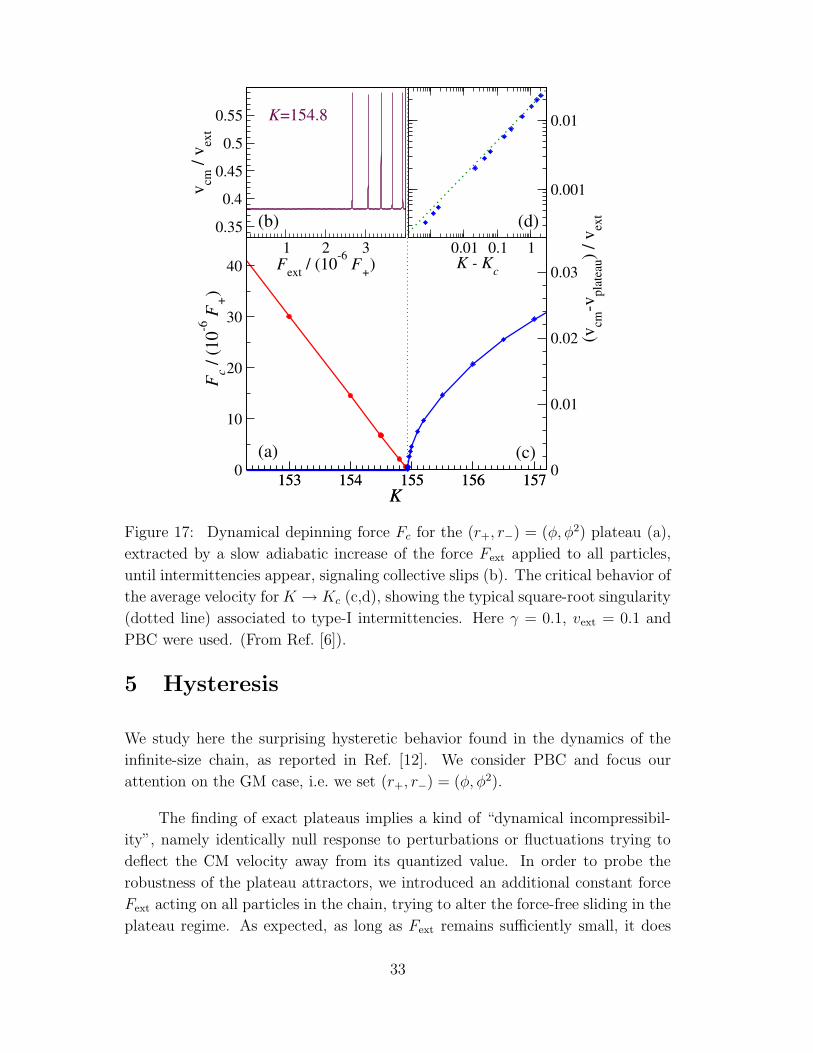
Figure 17: Dynamical depinning force Fc for the (r+, r−) = (φ, φ2) plateau (a),
extracted by a slow adiabatic increase of the force Fext applied to all particles,
until intermittencies appear, signaling collective slips (b). The critical behavior of
the average velocity for K → Kc (c,d), showing the typical square-root singularity
(dotted line) associated to type-I intermittencies. Here γ = 0.1, vext = 0.1 and
PBC were used. (From Ref. [6]).
5 Hysteresis
We study here the surprising hysteretic behavior found in the dynamics of the
infinite-size chain, as reported in Ref. [12]. We consider PBC and focus our
attention on the GM case, i.e. we set (r+, r−) = (φ, φ2).
The finding of exact plateaus implies a kind of “dynamical incompressibil-
ity”, namely identically null response to perturbations or fluctuations trying to
deflect the CM velocity away from its quantized value. In order to probe the
robustness of the plateau attractors, we introduced an additional constant force
Fext acting on all particles in the chain, trying to alter the force-free sliding in the
plateau regime. As expected, as long as Fext remains sufficiently small, it does
33

6.7 6.8 6.9Fext / (10-4 F+)
0.38
0.39
0.4
0.41
0.42
w =
vcm
/ v ex
tdecrease
increase
Figure 18: Hysteresis in the vcm-Fext characteristics for the GM case (r+, r−) =
(φ, φ2) and K = 120, inside the main plateau. Adiabatic increase and decrease
of Fext is denoted by triangles and circles, respectively. Here γ = 0.1, vext = 0.1
and PBC are applied.
perturb the single-particle motions but has no effect whatsoever on w, which
remains exactly pinned to the attractor (vcm ≡ vplateau). The plateau dynamics
is only abandoned above a critical force Fc. This picture is analogous to the
pinning-depinning transition in static friction, where a minimum force (the static
friction) is required in order to start the motion. Thus the sudden change of vcm
taking place at Fext = Fc can be termed a “dynamical depinning”: it takes place
through a series of type-I intermittencies [13], as shown in Fig. 17b, where vcm(t)
is plotted against a slow adiabatic ramping of Fext. The value of Fc is a nontrivial
function of the parameters, and vanishes linearly when K approaches from below
the upper border Kc of the plateau, as in Fig. 17a. The depinning transition line
Fc, ending at K = Kc, appears as a “first-order” line, with a jump ∆v in the
average vcm and an intriguing hysteretic behavior as Fext crosses Fc.
Fixing a value of the chain stiffness K inside the plateau of Fig. 9 and
34

considering a sufficiently small value of the damping coefficient γ (underdamped
regime), we investigate the hysteresis by applying an external force Fext to all the
chain particles through an adiabatic increase and decrease process. We choose an
initial value of the external force F inext below the critical value Fc, and increase it
by small steps ∆F . After each step, we leave sufficient time to the system in order
to reach its dynamical stationary state. In all calculations, the initial conditions
are obtained from the final conditions of the previous step. The same procedure is
used for the decrease process, starting with a value of F inext above Fc. The results
for K = 120 are shown in Fig. 18, where a clear hysteretic loop emerges: when
the applied force is decreased, the systems returns to the quantized sliding state
at a lower value of Fext with respect to the critical value Fc for which a jump ∆v
occurs in the increase process.
As can be expected, the jump ∆v and the force-width of the hysteresis
decrease to 0 as K increases towards Kc. Thus K = Kc represent a sort of non-
equilibrium critical point, where the sliding chain enters or leaves a dynamical
orbit. The precise value of Kc depends on parameters such as vext and γ; however,
its properties do not. As K approaches Kc from above (no external force), vcm
approaches vplateau in a critical manner, as suggested in Figs. 5 and 9. This is
detailed in Fig. 17c and 17d, where the critical behavior is shown to be ∆v ∝(K−Kc)
1/2, the value typical of intermittencies of type I [13]. In fact, for K & Kc
the chain spends most of its time moving at vcm(t) ' vplateau, except for short
bursts at regular time-intervals τ , where the system as a whole jumps ahead by
a0, i.e. by an extra chain lattice spacing (collective slip). The characteristic time
τ between successive collective slips diverges as τ ∝ (K − Kc)1/2 for K → Kc,
consistent with the critical behavior of w.
6 Conclusions
In this work, the velocity quantization phenomena recently found in the classical
motion of an idealized 1D solid lubricant have been related to the dynamics of
topological solitons (kinks). The plateau dynamics is explained by one slider
rigidly dragging the kinks that the chain forms with the other slider. We show
specifically that chains of finite and even small size, driven in between two periodic
sliders, move with characteristic quantized velocities, much like the infinite-size
ones do. Moreover, we find that a finite-size chain length re-adjusts in such a way
as to realize a lattice of kinks commensurate to the period of the smoother slider.
A consequence of this self-commensuration is a periodic single-particle oscillation,
35

even for incommensurate initial choices of the period ratios. We have also pointed
out that, in the finite-size model, size effects and boundary effects must be taken
into account with due care. In addition, we have shown that starting from the
quantized vcm sliding state, the layer sliding dynamics exhibits a clear hysteresis
under the action of an additional external driving force Fext, which attempts to
displace vcm away from its quantized value.
The phenomena reported for a model 1D system are quite extraordinary,
and it would be interesting if they could be observed in real systems. Nested
carbon nanotubes [14] are one possible arena for the phenomena considered here.
Though speculative at this stage, one obvious question is what aspects of the
phenomenology described might survive in two-dimensions (2D), where tribolog-
ical realizations, such as the sliding of two hard crystalline faces with, e.g., an
interposed graphite flake, are conceivable. Our results suggest that the lattice of
discommensuration (a Moire pattern), formed by the flake on a substrate, could
be dragged by the other sliding crystal face, in such a manner that the speed of the
flake as a whole would be smaller, and quantized. Dienwiebel et al. [15] demon-
strated how incommensurability may lead to virtually friction-free sliding in such
a case, but no measure was obtained for the flake relative sliding velocity. Real
substrates are, unlike our model, not rigid, subject to thermal expansion, and
defected. Nevertheless, the ubiquity of plateaus (see Fig. 5 and Fig. 10), their
topological origin, their continuous dependence on the length ratios, and their
persistence in finite-size samples suggest that these effects would not remove the
phenomenon, which should therefore be accessible experimentally.
The results of the present thesis are partially included in Ref. [12], and
mainly in Ref. [16].
36

References
[1] O.M. Braun and Y.S. Kivshar, The Frenkel-Kontorova Model: Concepts,
Methods, and Applications (Springer-Verlag, Berlin, 2004).
[2] M. Peyrand, and S. Aubry, J. Phys. C: Solid State Phys. 16, 1593 (1983).
[3] R. Besseling, R. Niggebrugge, and P.H. Kes, Phys. Rev. Lett. 82, 3144 (1999).
[4] L. Trallori, Phys. Rev. B 57, 5923 (1998).
[5] M. Porto, M. Urbakh, and J. Klafter, Phys. Rev. Lett. 84, 6058 (2000).
[6] A. Vanossi, N. Manini, G. Divitini, G.E. Santoro, and E. Tosatti, Phys. Rev.
Lett. 97, 056101 (2006).
[7] G.E. Santoro, A. Vanossi, N. Manini, G. Divitini, and E. Tosatti, Surf. Sci.
600, 2726 (2006).
[8] A. Vanossi, J. Roeder, A.R. Bishop, and V. Bortolani, Phys. Rev. E 63,
017203 (2001).
[9] A. Vanossi, J. Roeder, A.R. Bishop, and V. Bortolani, Phys. Rev. E 67,
016606 (2003).
[10] O.M. Braun, A. Vanossi, and E. Tosatti, Phys. Rev. Lett. 95, 026102 (2005)
[11] W.H. Press, S.A. Teukolsky, W.T. Vetterling, and B.P. Flannery, NUMER-
ICAL RECIPES in C++. The Art of Scientific Computing (Cambridge Uni-
versity Press, 2002).
[12] A. Vanossi, G.E. Santoro, N. Manini, M. Cesaratto, and E. Tosatti, cond-
mat/0609117, submitted to Surf. Sci.
[13] P. Berge, Y. Pomeau, and C. Vidal, Order within Chaos (Hermann and John
Wiley & Sons, Paris, 1984).
[14] X.H. Zhang, U. Tartaglino, G.E. Santoro, and E. Tosatti, submitted to
Surf. Sci.
[15] M. Dienwiebel, G.S. Verhoeven, N. Pradeep, J.W.M. Frenken, J.A. Heim-
berg, and H.W. Zandbergen, Phys. Rev. Lett. 92, 126101 (2004).
[16] M. Cesaratto, N. Manini, A. Vanossi, E. Tosatti, and G.E. Santoro, cond-
mat/0609116, submitted to Surf. Sci.
37


