IV. CUMULATIVE DAMAGE LEADING TO FATIGUE AND CREEP FAILURE FOR
GENERAL MATERIALS
Of the various headings under mechanics of materials, failure is usually
considered to be the most difficult one. Then proceeding further to the sub-
fields under failure, probably fatigue is considered to be its most difficult one.
The concept of damage comes into play with fatigue, but deducing useful and
reasonably general damage forms has been a taxing and uncertain exercise.
The organized attempts to quantify damage usually fall under the subject of
cumulative damage with the understanding that the damage leads to and
terminates with materials failure.
Quantifying damage relative to failure allows the optimization of stress
loading programs and allows the means for including overload type damage
events. Although this website is not aimed as a literature survey, this section
will be used to examine several different approaches for cumulative damage.
The possible applications are to isotropic or anisotropic materials (including
composites) with the proviso that in either case the conditions of proportional
loading apply.
Creep rupture also comes under the heading of cumulative damage. Creep
rupture is the time dependent damage growth leading to failure in polymers
and in metals at high temperature. As developed here, fatigue conditions and
creep rupture conditions admit the same general formulation. Both will be
treated and with suitable notational changes either form can be found from the
other.
There are considered to be two main approaches for cumulative damage.
One is that of the direct postulation of lifetime damage forms such as Miner’s
rule and the other is that of residual strength. Residual strength is the reduced
(instantaneous) static strength that the material can still deliver after being
subjected to loads causing damage. Of course both are relevant to the general
problem and a well founded cumulative damage theory must contain both
descriptions in a compatible form. The overall objective of both and of all
approaches is to secure a life prediction methodology.
In the area of the fatigue of metals, a common approach is to assume a pre-
existing crack that grows according to a power law form with regard to the
stress level. This is often called the Paris law. When the crack reaches a
certain pre-specified size, the service life is considered to be completed.
While this is certainly a useful approach it cannot be considered to be a life
prediction methodology based upon the approach to failure. Accordingly it
will not be followed here.
The general topics of fatigue or of damage are covered in many self
contained, inclusive books such as Suresh [1] and Krajcinovic [ 2]. As part of
a general damage approach, constitutive relations are often taken for damage
involving scalar or tensor valued damage variables and a whole framework of
behavior is built up. In a considerably different direction to be followed here,
cumulative damage leading to failure is more akin to failure criteria, but with
the capability to characterize damage as the prelude to failure. The first
credible damage form was that of Miner’s rule [3]. Broutman and Sahu [4]
and Hashin and Rotem [5] much later produced other damage forms that
with the passage of time have gained credibility. Reifsnider [6] initiated a
different damage formalism which has been further developed by him and
others in other papers. Other also notable efforts have been given by Adam et
al [7] and by many other workers. Christensen [8] recently developed a new
and different approach. Post, Case, and Lesko [9] have recently given a
survey of many different cumulative damage models and applied them to
situations of spectrum type loadings for composites.
Due to the complexity of the topic many approaches and models contain
adjustable parameters, sometimes many parameters. In the coverage
undertaken here only models without any adjustable parameters will be
considered. That is to say, the damage formulations to be considered will be
based solely upon the properties contained within a database of constant
amplitude fatigue or creep testing and the static strength. Then the damage
forms will be used to predict life under variable amplitude programs of load
application. This circumstance is analogous to viscoelastic behavior where
mechanical properties of creep or relaxation function type are inserted into
convolution integrals to predict general behavior. Materials with memory
could encompass viscoelastic effects at one extreme, and damage memory
effects at the other extreme. The four damage models to be examined here are
those of Miner’s rule, Hashin-Rotem, Broutman-Sahu, and then the recently
developed one by Christensen. The Broutman-Sahu form is representative of
a large class of models, as will be explained later.
In terms of evaluating damage models, there does not appear to be any
definitive set or sets of experimental data. The problem is the lack of
repeatability and in a more general sense the great variability in the data. This
places even more emphasis on the need for a careful theoretical evaluation,
looking for physical consistency in the predictions and conversely examining
aspects of inconsistency in important special cases.
Three main problems will be used to evaluate the four models. These
include examples of prescribed major damage followed by the predicted life at
a lower, safer stress level. Another problem is that of the ability to predict
residual instantaneous strength after a long time load application that
nevertheless is shorter than that time which would cause fatigue or creep
failure. Thirdly is the problem of residual life. In this situation a load is
applied right up to the time of, but just an instant before, fatigue or creep
failure. At that time the load is removed and replaced by one of a lower, less
stringent level. The additional life that results at the lower stress level is
designated as the residual life.
All of these models and methods are taken from the peer reviewed literature.
The new dimension which is added here is that of a more inclusive theoretical
evaluation than appears to have been previously given.
Four Alternative Approaches
The general concept of damage that would or could lead to failure was
rather vague and nebulous until Miner gave it a specific form and it became
recognized. With background from Palmgren, Miner [3] postulated the
damage form for fatigue as
!
ni
Nii
" = 1 (1)
where ni is the number of applied cycles at nominal stress !i and Ni is the
limit number of cycles to failure at the same stress and for the same cycle
type. Thus each value ni/Ni is viewed as a quanta of damage, the sum of
which specifies failure. As with all cumulative damage forms, when the left
hand side of (1) is less than one, it still quantifies the damage level but does
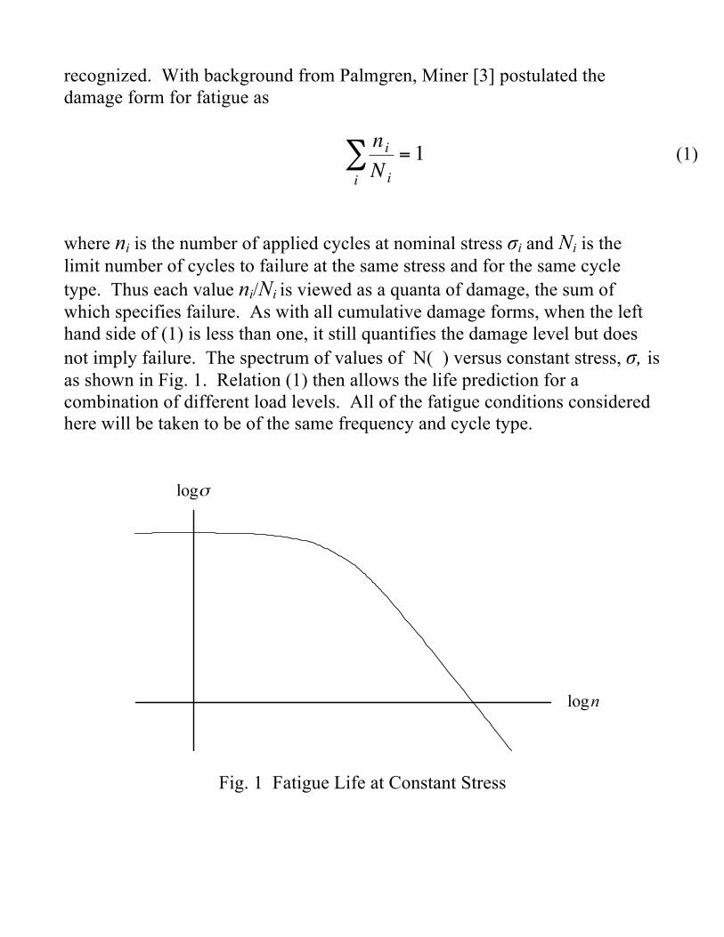
not imply failure. The spectrum of values of N( ) versus constant stress, !, is
as shown in Fig. 1. Relation (1) then allows the life prediction for a
combination of different load levels. All of the fatigue conditions considered
here will be taken to be of the same frequency and cycle type.
Fig. 1 Fatigue Life at Constant Stress
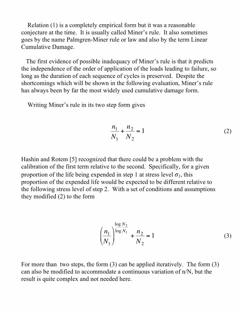
Relation (1) is a completely empirical form but it was a reasonable
conjecture at the time. It is usually called Miner’s rule. It also sometimes
goes by the name Palmgren-Miner rule or law and also by the term Linear
Cumulative Damage.
The first evidence of possible inadequacy of Miner’s rule is that it predicts
the independence of the order of application of the loads leading to failure, so
long as the duration of each sequence of cycles is preserved. Despite the
shortcomings which will be shown in the following evaluation, Miner’s rule
has always been by far the most widely used cumulative damage form.
Writing Miner’s rule in its two step form gives
!
n1
N1
+n2
N2
= 1 (2)
Hashin and Rotem [5] recognized that there could be a problem with the
calibration of the first term relative to the second. Specifically, for a given
proportion of the life being expended in step 1 at stress level !1, this
proportion of the expended life would be expected to be different relative to
the following stress level of step 2. With a set of conditions and assumptions
they modified (2) to the form
!
n1
N1
"
# $
%
& '
log N2
log N1+n2
N 2
= 1 (3)
For more than two steps, the form (3) can be applied iteratively. The form (3)
can also be modified to accommodate a continuous variation of n/N, but the
result is quite complex and not needed here.
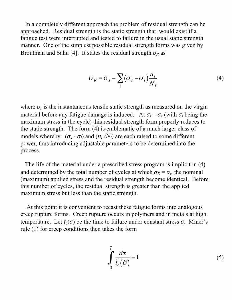
In a completely different approach the problem of residual strength can be
approached. Residual strength is the static strength that would exist if a
fatigue test were interrupted and tested to failure in the usual static strength
manner. One of the simplest possible residual strength forms was given by
Broutman and Sahu [4]. It states the residual strength !R as
!
"R
="s# "
s#"
i( )i
$ni
Ni
(4)
where !s is the instantaneous tensile static strength as measured on the virgin
material before any fatigue damage is induced. At !i = !s (with !i being the
maximum stress in the cycle) this residual strength form properly reduces to
the static strength. The form (4) is emblematic of a much larger class of
models whereby (!s - !i) and (ni /Ni) are each raised to some different
power, thus introducing adjustable parameters to be determined into the
process.
The life of the material under a prescribed stress program is implicit in (4)
and determined by the total number of cycles at which !R = !i, the nominal
(maximum) applied stress and the residual strength become identical. Before
this number of cycles, the residual strength is greater than the applied
maximum stress but less than the static strength.
At this point it is convenient to recast these fatigue forms into analogous
creep rupture forms. Creep rupture occurs in polymers and in metals at high
temperature. Let tc(!) be the time to failure under constant stress !. Miner’s
rule (1) for creep conditions then takes the form
!
d"
˜ t c
˜ # ( )=1
0
˜ t
$ (5)
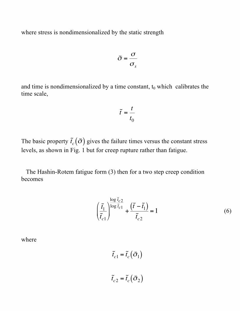
where stress is nondimensionalized by the static strength
!
˜ " ="
"s
and time is nondimensionalized by a time constant, t0 which calibrates the
time scale,
!
˜ t =t
t0
The basic property
!
˜ t c
˜ " ( ) gives the failure times versus the constant stress
levels, as shown in Fig. 1 but for creep rupture rather than fatigue.
The Hashin-Rotem fatigue form (3) then for a two step creep condition
becomes
!
˜ t 1
˜ t c1
"
# $
%
& '
log ˜ t c2
log ˜ t c1+
˜ t ( ˜ t 1( )˜ t c2
=1 (6)
where
!
˜ t c1
= ˜ t c
˜ " 1( )
!
˜ t c2
= ˜ t c
˜ " 2( )
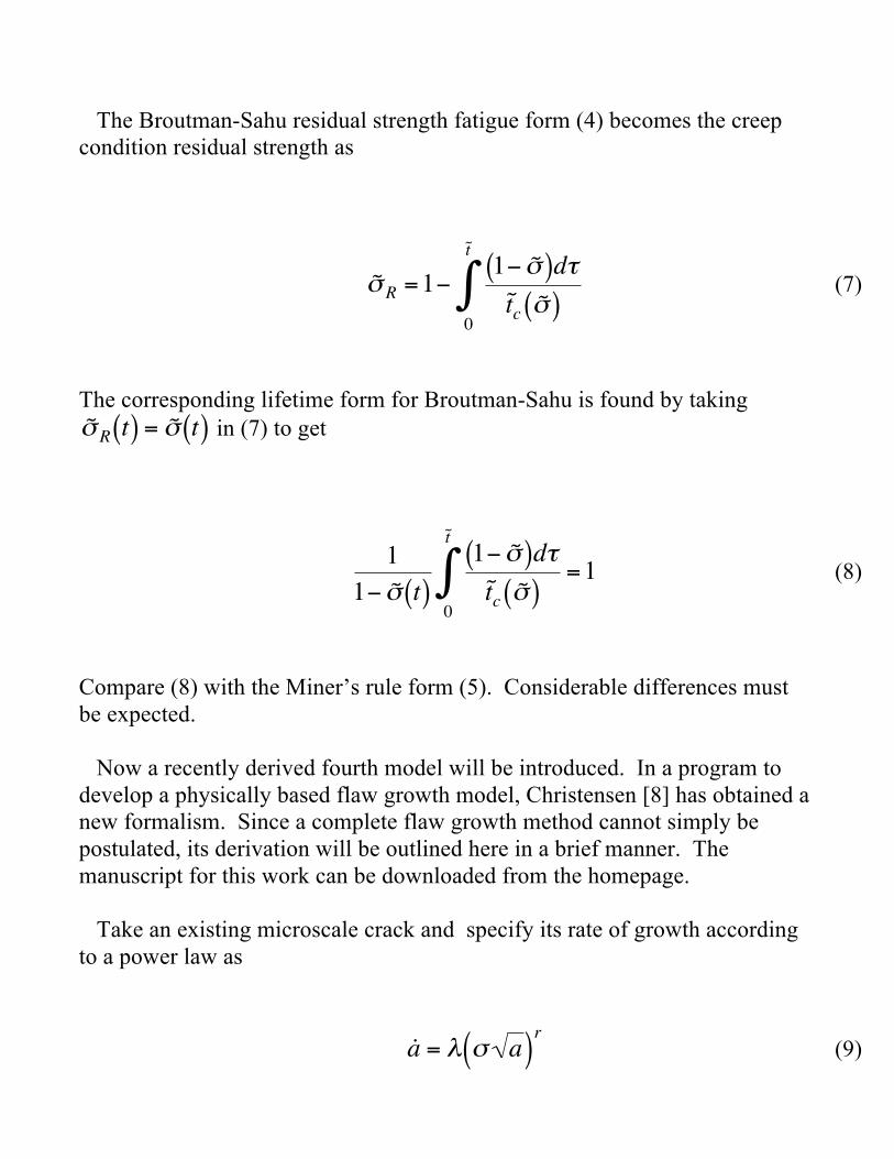
The Broutman-Sahu residual strength fatigue form (4) becomes the creep
condition residual strength as
!
˜ " R
=1#1# ˜ " ( )d$
˜ t c
˜ " ( )0
˜ t
% (7)
The corresponding lifetime form for Broutman-Sahu is found by taking
!
˜ " Rt( ) = ˜ " t( ) in (7) to get
!
1
1" ˜ # t( )
1" ˜ # ( )d$˜ t c
˜ # ( )=1
0
˜ t
% (8)
Compare (8) with the Miner’s rule form (5). Considerable differences must
be expected.
Now a recently derived fourth model will be introduced. In a program to
develop a physically based flaw growth model, Christensen [8] has obtained a
new formalism. Since a complete flaw growth method cannot simply be
postulated, its derivation will be outlined here in a brief manner. The
manuscript for this work can be downloaded from the homepage.
Take an existing microscale crack and specify its rate of growth according
to a power law as
!
˙ a = " # a( )r
(9)
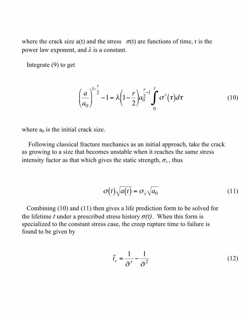
where the crack size a(t) and the stress !(t) are functions of time, r is the
power law exponent, and " is a constant.
Integrate (9) to get
!
a
a0
"
# $
%
& '
1(r
2
(1= ) 1(r
2
"
# $
%
& ' a0
r
2(1
* r
0
t
+ ,( )d, (10)
where a0 is the initial crack size.
Following classical fracture mechanics as an initial approach, take the crack
as growing to a size that becomes unstable when it reaches the same stress
intensity factor as that which gives the static strength, !s , thus
!
" t( ) a t( ) = "sa0
(11)
Combining (10) and (11) then gives a life prediction form to be solved for
the lifetime t under a prescribed stress history !(t). When this form is
specialized to the constant stress case, the creep rupture time to failure is
found to be given by
!
˜ t c
=1
˜ " r#
1
˜ " 2 (12)
where nondimensional stress and nondimensional time will be used from this
point on. Relation (12) has a behavior as shown in the first case of Fig. 2
below on log-log scales. At long time there is a power law behavior
controlled by the exponent r and at short time it approaches the static strength
asymptote. That much is perfectly acceptable. However, the form (12)
exhibits a rather sharp transition from one asymptote to the other. Most data
show a more gradual transition. Thus a more general approach is required ,
although the form (12) could remain as a special case. The single, isolated,
ideal crack is of limited value in understanding the explicit failure of
homogeneous materials. It gives useful, qualitative guidelines but not the
concrete, quantitative results that can be used in applications.
Going back to relation (11) which gives the criterion for unstable growth of
the crack, it must be considered as being inadequate. Instead, replace (11) by
the more general form
!
˜ a = F ˜ " ( ) (13)
where
!
˜ a = a t( ) /a0
and F( ) is a function of stress yet to be determined. The necessity for this
generalization beyond the behavior of a single ideal crack relates to more
complex matters such as the possible interaction between cracks, crack
coalescence and many other non-ideal types of damage and damage growth.
The basic flaw growth relation (9) will be retained, but now a(t) represents
some more general measure of flaw size as it grows.
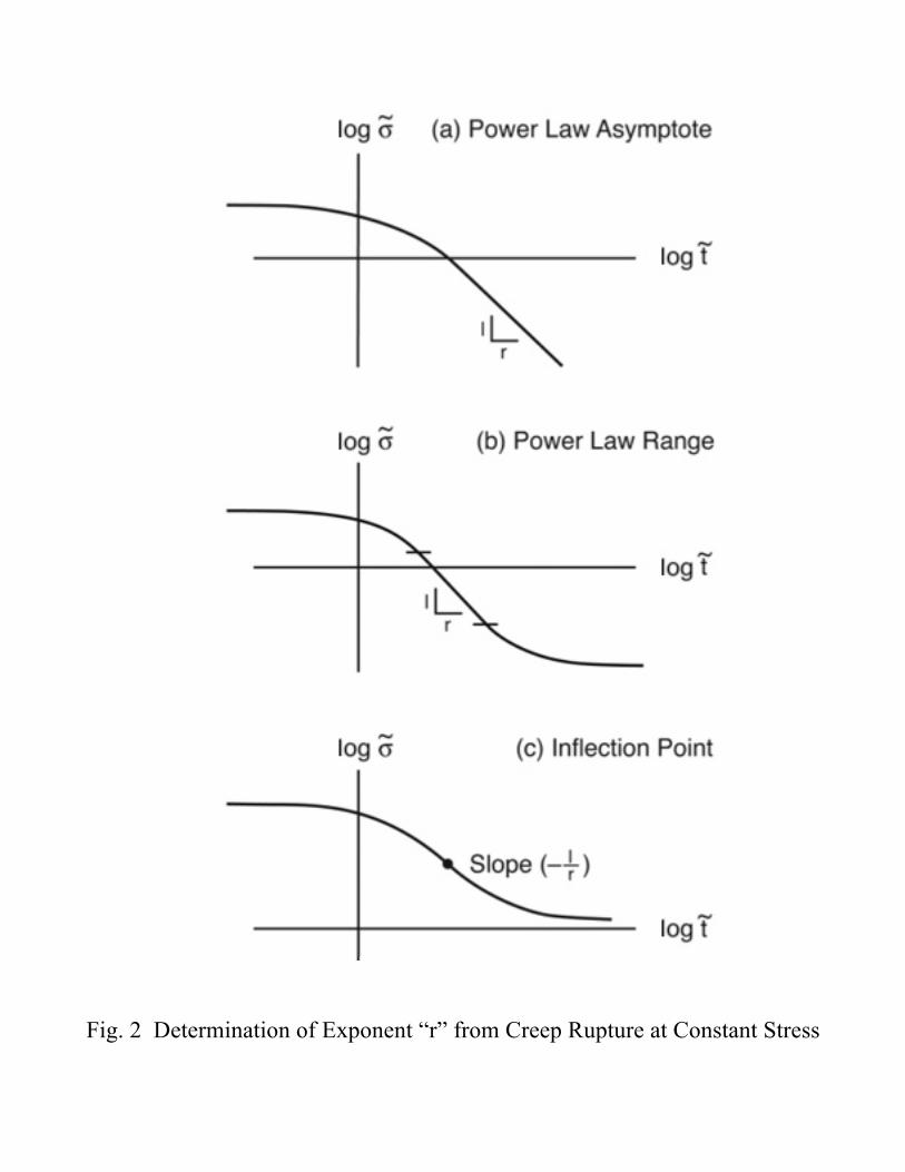
Fig. 2 Determination of Exponent “r” from Creep Rupture at Constant Stress
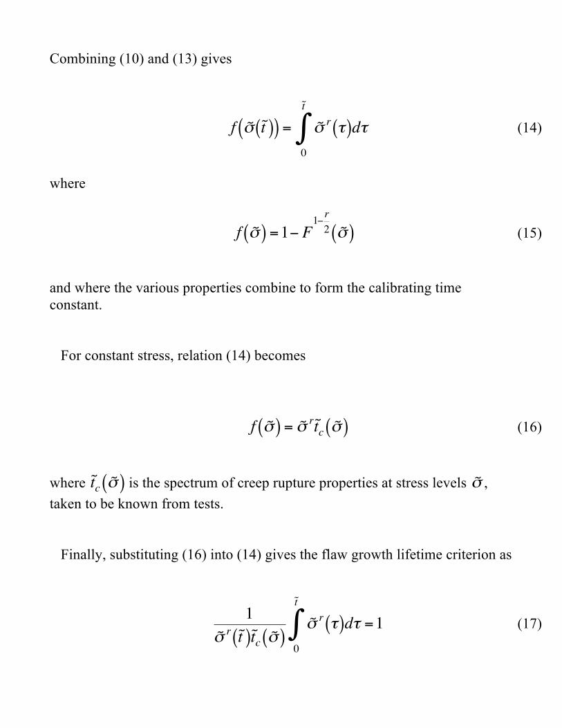
Combining (10) and (13) gives
!
f ˜ " ˜ t ( )( ) = ˜ " r
0
˜ t
# $( )d$ (14)
where
!
f ˜ " ( ) =1# F1#r
2 ˜ " ( ) (15)
and where the various properties combine to form the calibrating time
constant.
For constant stress, relation (14) becomes
!
f ˜ " ( ) = ˜ " r ˜ t c ˜ " ( ) (16)
where
!
˜ t c
˜ " ( ) is the spectrum of creep rupture properties at stress levels
!
˜ " ,
taken to be known from tests.
Finally, substituting (16) into (14) gives the flaw growth lifetime criterion as
!
1
˜ " r ˜ t ( )˜ t c
˜ " ( )˜ " r
0
˜ t
# $( )d$ =1 (17)
For a given stress history
!
˜ " #( ) , relation (17) determines the lifetime,
!
˜ t , of
the material. The exponent r is determined from the basic creep rupture
forms as shown in Fig. 2. The creep rupture properties and its specific
property r calibrate the theory behind the life prediction form (17). It is not
surprising that the property
!
˜ t c
˜ " ( ) in (17) is at current time,
!
˜ t , rather than
being inside the integral as in the other models. This relates to the method
whereby the flaw grows until it reaches a critical size at the then existing
current stress. This present approach also admits a full statistical
generalization, see Christensen [8]. The manuscript of this published work
can be downloaded from the www.FailureCriteria.com homepage.
The four basic forms under consideration here, Miner’s rule, Hashin-Rotem,
Broutman-Sahu, and the present form are respectively given by (5), (6), (8),
and (17), It is important to observe that all of these are completely calibrated
by and determined by only the basic experimentally determined creep rupture
property
!
˜ t c
˜ " ( ) and the static strength. There are no additional parameters to
be adjusted or fine tuned. Apparently these four are the only forms that have
been proposed or derived that do not involve additional parameters beyond the
mechanical properties.
It is interesting to note that there is a special case in which two of these
basic forms become identical. Specifically for a creep rupture property of the
power law type, as in
!
˜ t c
=A
˜ " r (18)
then Miner’s rule (5) and the present form (17) reduce to the same form. This
is shown directly by substituting (18) into each of these. Otherwise these two
forms make completely different predictions, sometimes extremely different
predictions. In this power law special case, (18), the creep rupture conforms
to the limiting (degenerate) case show in Fig. 3.
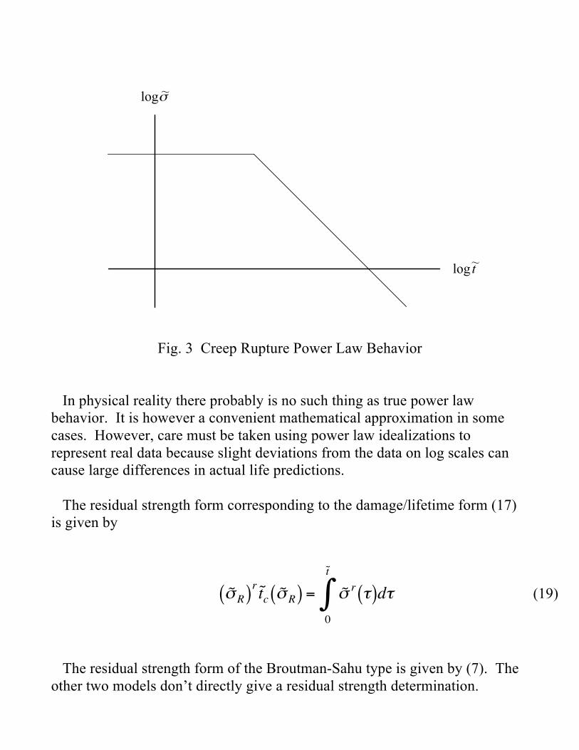
Fig. 3 Creep Rupture Power Law Behavior
In physical reality there probably is no such thing as true power law
behavior. It is however a convenient mathematical approximation in some
cases. However, care must be taken using power law idealizations to
represent real data because slight deviations from the data on log scales can
cause large differences in actual life predictions.
The residual strength form corresponding to the damage/lifetime form (17)
is given by
!
˜ " R( )
r˜ t c
˜ " R( ) = ˜ " r
0
˜ t
# $( )d$ (19)
The residual strength form of the Broutman-Sahu type is given by (7). The
other two models don’t directly give a residual strength determination.
The fatigue life forms for the first two models are given by Miner’s rule (1)
and Hashin-Rotem (3). The Broutman-Sahu form for fatigue life is given
from (4) by setting !R = !i . The fatigue life form from the present derivation
is given by
!
1
"K( )
rN "
K( )"i( )r
i=1
K
# ni=1 (20)
where exponent r is given by the basic fatigue property envelope at constant
amplitude, the same as in the creep rupture curves of Fig. 2.
This completes the background and specification of the four basic forms
under consideration. Now a comparative evaluation of these forms will be
given using the creep failure notation.
Residual Strength
When a general program of stress history is interrupted and suddenly tested
for static strength, Fig. 4, the residual strength, !R , is determined.
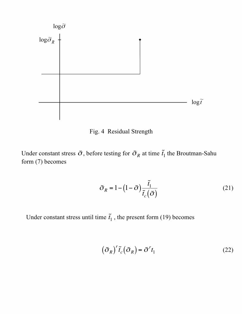
Fig. 4 Residual Strength
Under constant stress
!
˜ " , before testing for
!
˜ " R
at time
!
˜ t 1 the Broutman-Sahu
form (7) becomes
!
˜ " R
=1# 1# ˜ " ( )˜ t 1
˜ t c
˜ " ( ) (21)
Under constant stress until time
!
˜ t 1 , the present form (19) becomes
!
˜ " R( )
r˜ t c
˜ " R( ) = ˜ " rt
1 (22)
To determine
!
˜ " R
from (22) requires knowledge of the range of values for
!
˜ t c
˜ " R( ) . In contrast (21) only requires knowledge of the value of
!
˜ t c at one
value of stress. This difference has important implications as will be seen
next.
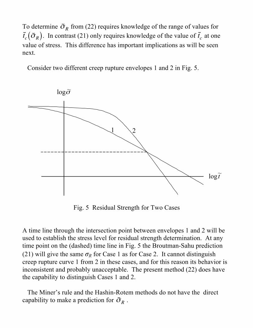
Consider two different creep rupture envelopes 1 and 2 in Fig. 5.
Fig. 5 Residual Strength for Two Cases
A time line through the intersection point between envelopes 1 and 2 will be
used to establish the stress level for residual strength determination. At any
time point on the (dashed) time line in Fig. 5 the Broutman-Sahu prediction
(21) will give the same !R for Case 1 as for Case 2. It cannot distinguish
creep rupture curve 1 from 2 in these cases, and for this reason its behavior is
inconsistent and probably unacceptable. The present method (22) does have
the capability to distinguish Cases 1 and 2.
The Miner’s rule and the Hashin-Rotem methods do not have the direct
capability to make a prediction for
!
˜ " R
.
Damage/Life Examples
Another useful way to compare the models is to consider the remaining life
after a major damage event. To simulate this, a two step loading program will
be taken with the first step, of specified duration, being at a high stress
overload, and the second step consisting of the service level stress up to
failure.
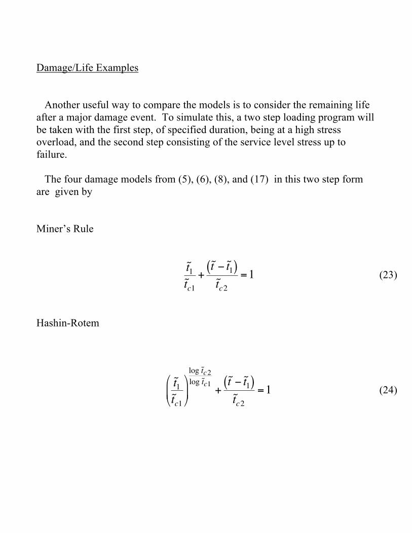
The four damage models from (5), (6), (8), and (17) in this two step form
are given by
Miner’s Rule
!
˜ t 1
˜ t c1
+˜ t " ˜ t
1( )˜ t c2
=1 (23)
Hashin-Rotem
!
˜ t 1
˜ t c1
"
# $
%
& '
log ˜ t c2
log ˜ t c1+
˜ t ( ˜ t 1( )˜ t c2
=1 (24)
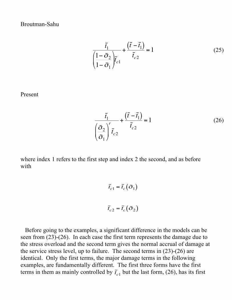
Broutman-Sahu
!
˜ t 1
1" ˜ # 2
1" ˜ # 1
$
% &
'
( ) ̃ t
c1
+˜ t " ˜ t
1( )˜ t c2
=1 (25)
Present
!
˜ t 1
˜ " 2
˜ " 1
#
$ %
&
' (
r
˜ t c2
+˜ t ) ˜ t
1( )˜ t c2
=1 (26)
where index 1 refers to the first step and index 2 the second, and as before
with
!
˜ t c1
= ˜ t c
˜ " 1( )
!
˜ t c2
= ˜ t c
˜ " 2( )
Before going to the examples, a significant difference in the models can be
seen from (23)-(26). In each case the first term represents the damage due to
the stress overload and the second term gives the normal accrual of damage at
the service stress level, up to failure. The second terms in (23)-(26) are
identical. Only the first terms, the major damage terms in the following
examples, are fundamentally different. The first three forms have the first
terms in them as mainly controlled by
!
˜ t c1
but the last form, (26), has its first
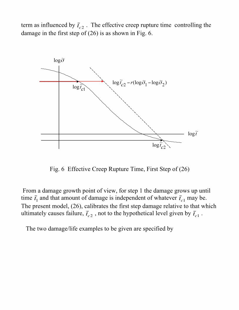
term as influenced by
!
˜ t c2
. The effective creep rupture time controlling the
damage in the first step of (26) is as shown in Fig. 6.
Fig. 6 Effective Creep Rupture Time, First Step of (26)
From a damage growth point of view, for step 1 the damage grows up until
time
!
˜ t 1 and that amount of damage is independent of whatever
!
˜ t c1
may be.
The present model, (26), calibrates the first step damage relative to that which
ultimately causes failure,
!
˜ t c2
, not to the hypothetical level given by
!
˜ t c1
.
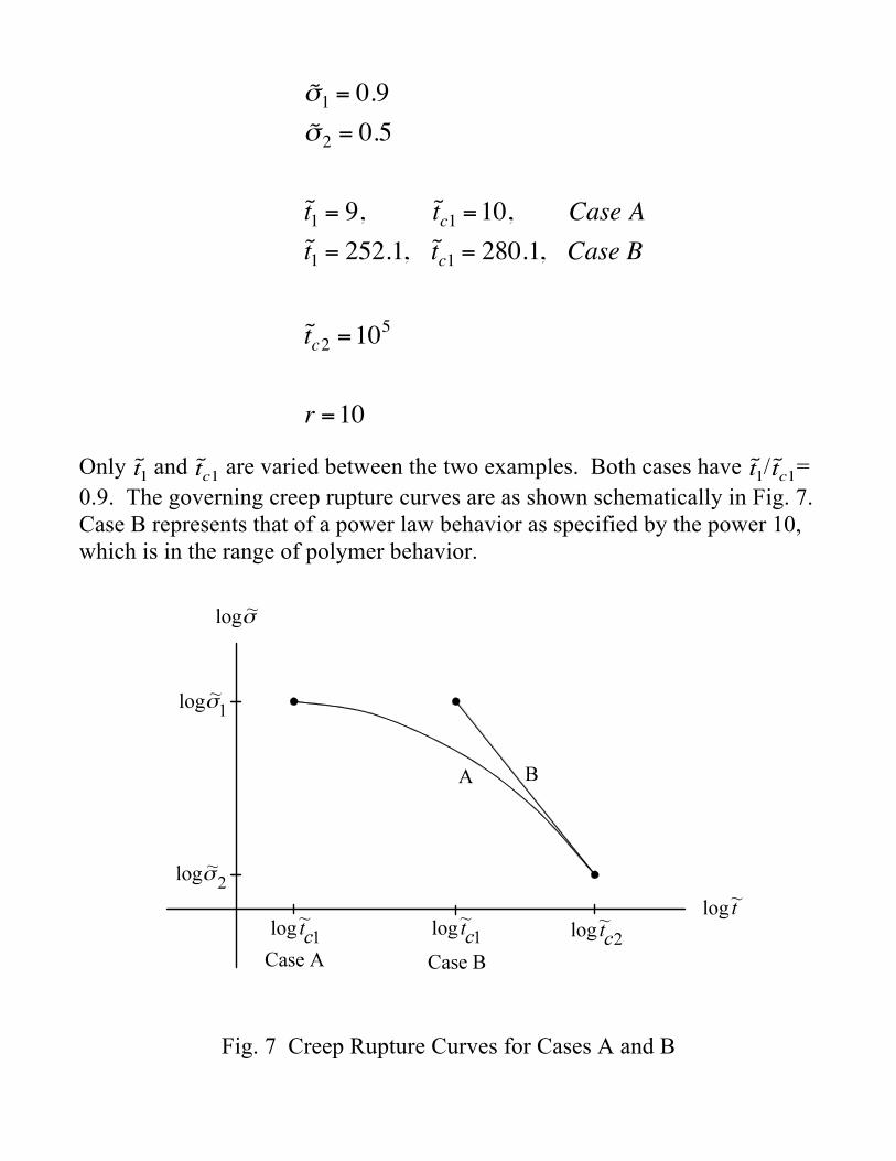
The two damage/life examples to be given are specified by
!
˜ " 1 = 0.9
˜ " 2 = 0.5
˜ t 1 = 9, ˜ t c1 =10, Case A
˜ t 1 = 252.1, ˜ t c1 = 280.1, Case B
˜ t c2 =10
5
r =10
Only
!
˜ t 1 and
!
˜ t c1
are varied between the two examples. Both cases have
!
˜ t 1/
!
˜ t c1
=
0.9. The governing creep rupture curves are as shown schematically in Fig. 7.
Case B represents that of a power law behavior as specified by the power 10,
which is in the range of polymer behavior.
Fig. 7 Creep Rupture Curves for Cases A and B
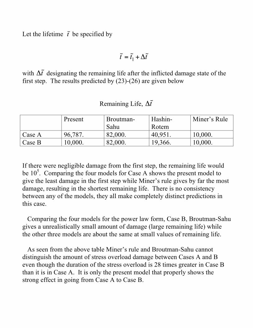
Let the lifetime
!
˜ t be specified by
!
˜ t = ˜ t 1+"˜ t
with
!
"˜ t designating the remaining life after the inflicted damage state of the
first step. The results predicted by (23)-(26) are given below
Remaining Life,
!
"˜ t
Present Broutman-
Sahu
Hashin-
Rotem
Miner’s Rule
Case A 96,787. 82,000. 40,951. 10,000.
Case B 10,000. 82,000. 19,366. 10,000.
If there were negligible damage from the first step, the remaining life would
be 105. Comparing the four models for Case A shows the present model to
give the least damage in the first step while Miner’s rule gives by far the most
damage, resulting in the shortest remaining life. There is no consistency
between any of the models, they all make completely distinct predictions in
this case.
Comparing the four models for the power law form, Case B, Broutman-Sahu
gives a unrealistically small amount of damage (large remaining life) while
the other three models are about the same at small values of remaining life.
As seen from the above table Miner’s rule and Broutman-Sahu cannot
distinguish the amount of stress overload damage between Cases A and B
even though the duration of the stress overload is 28 times greater in Case B
than it is in Case A. It is only the present model that properly shows the
strong effect in going from Case A to Case B.
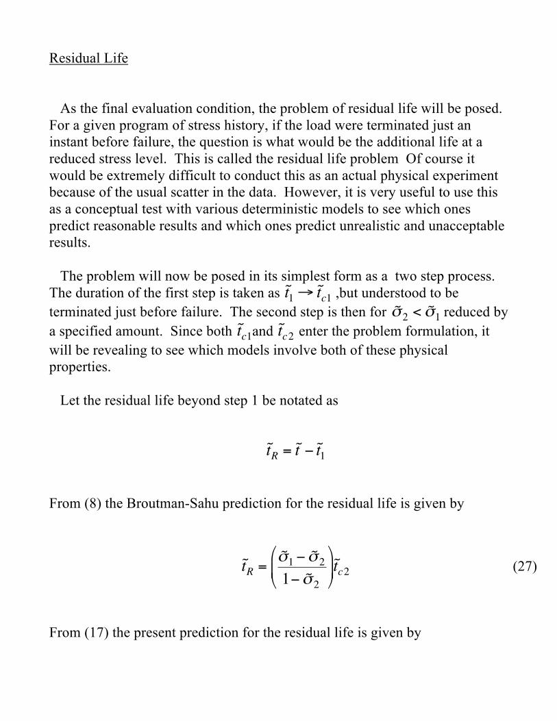
Residual Life
As the final evaluation condition, the problem of residual life will be posed.
For a given program of stress history, if the load were terminated just an
instant before failure, the question is what would be the additional life at a
reduced stress level. This is called the residual life problem Of course it
would be extremely difficult to conduct this as an actual physical experiment
because of the usual scatter in the data. However, it is very useful to use this
as a conceptual test with various deterministic models to see which ones
predict reasonable results and which ones predict unrealistic and unacceptable
results.
The problem will now be posed in its simplest form as a two step process.
The duration of the first step is taken as
!
˜ t 1" ˜ t
c1 ,but understood to be
terminated just before failure. The second step is then for
!
˜ " 2
< ˜ " 1 reduced by
a specified amount. Since both
!
˜ t c1
and
!
˜ t c2
enter the problem formulation, it
will be revealing to see which models involve both of these physical
properties.
Let the residual life beyond step 1 be notated as
!
˜ t R
= ˜ t " ˜ t 1
From (8) the Broutman-Sahu prediction for the residual life is given by
!
˜ t R
=˜ "
1# ˜ "
2
1# ˜ " 2
$
% &
'
( ) ̃ t
c2 (27)
From (17) the present prediction for the residual life is given by
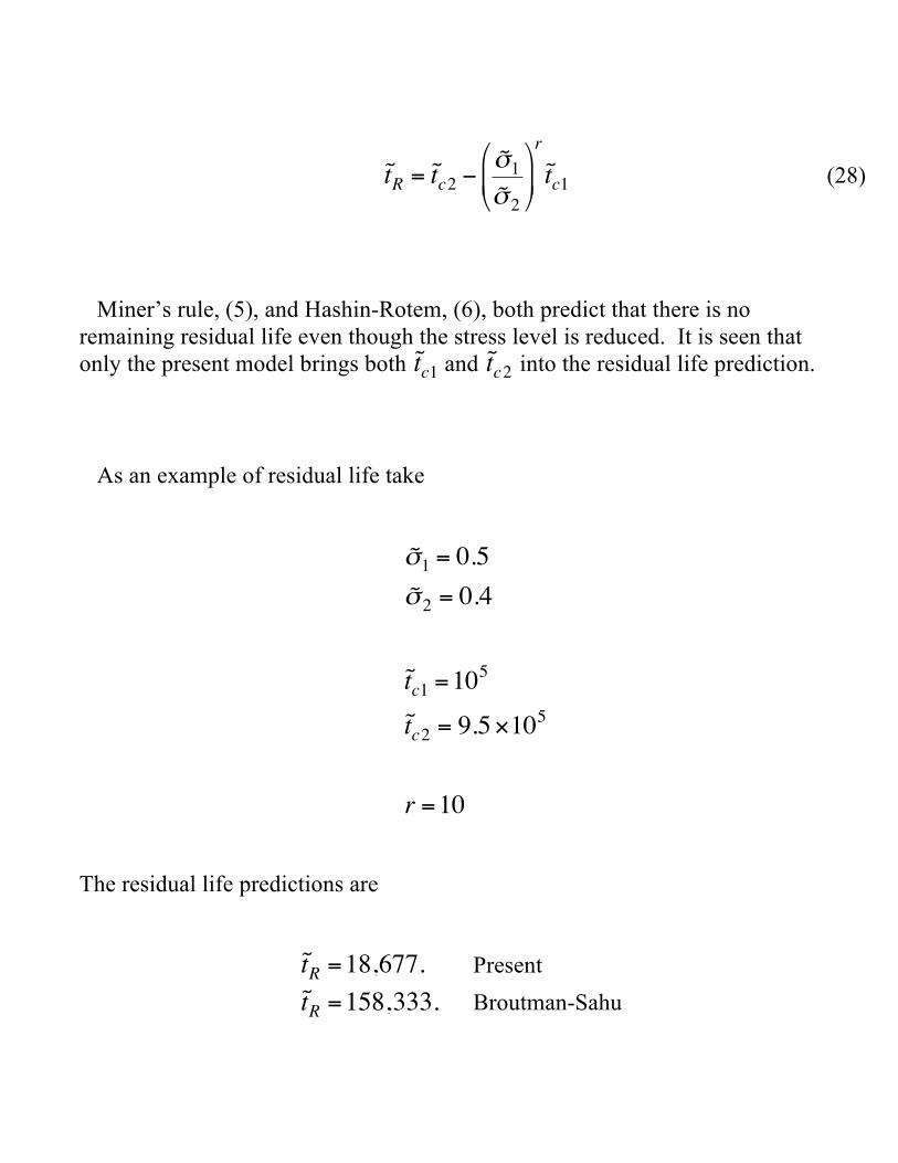
!
˜ t R
= ˜ t c2"
˜ # 1
˜ # 2
$
% &
'
( )
r
˜ t c1
(28)
Miner’s rule, (5), and Hashin-Rotem, (6), both predict that there is no
remaining residual life even though the stress level is reduced. It is seen that
only the present model brings both
!
˜ t c1
and
!
˜ t c2
into the residual life prediction.
As an example of residual life take
!
˜ " 1
= 0.5
˜ " 2
= 0.4
˜ t c1
=105
˜ t c2
= 9.5#105
r =10
The residual life predictions are
!
˜ t R
=18,677. Present
!
˜ t R
=158,333. Broutman-Sahu
Conclusion
The three model testing conditions: damage/life, residual strength, and
residual life, show that the present model is the only one of the four that
satisfies these consistency tests. More specifically, the damage/life examples
reveal the importance of the maximum slope of the creep rupture-life
envelope on log-log scales, Fig. 2. Only the present model includes this
characteristic, as property r in (17). This property is important because it
calibrates the kinetics of the flaw growth process. Without this defining
property, two points on a stress versus life envelope cannot distinguish power
law behavior from anything else. It is analogous to trying to define curvature
by only two points. With this property included, it can be shown from (17)
that in general for two step programs of loading, the high stress to low stress
sequence produces longer lifetimes than does the low to high sequence.
General observations usually confirm this specific sequence effect, Found and
Quaresimin [10]. Miner’s rule says there is no sequence effect. Interested
readers could examine other models and deduce other conditions of evaluation
in addition to those considered here.
References
[1] Suresh, S., 1998, Fatigue of Materials, 2nd
ed., Cambridge Univ. Press.
[2] Krajcinovic, D., 1996, Damage Mechanics, Elsevier.
[3] Miner, M. A., 1945, “Cumulative Damage in Fatigue,” J. Applied
Mechanics, 12, A159-A164.
[4] Broutman, L. J. and Sahu, S., 1972, “A New Theory to Predict
Cumulative Damage in Fiberglass Reinforced Composites,” in Composite
Materials Testing and Design, ASTM STP 497, 170-188.
[5] Hashin, Z., and Rotem, A., 1978, “A Cumulative Damage Theory of
Fatigue Failure, Mats. Sci and Eng., 34, 147-160.
[6] Reifsnider, K. L., 1986, “The Critical Element Model: A Modeling
Philosophy,” Eng. Frac. Mech., 25, 739-749.
[7] Adam, T., Dickson, R. F., Jones, C. J., Reiter, H., and Harris, B., 1986,
“A Power Law Fatigue Damage Model for Fibre-Reinforced Plastic
Laminates,” Pro. Inst. Mech. Engrs., 200, 155-165.
[8] Christensen, R. M., 2008, “A Physically Based Cumulative Damage
Formalism,” Int. J. Fatigue, 30, 595-602.
[9] Post, N. L., Case, S. W., and Lesko, J. J., 2008, “Modeling the Variable
Amplitude Fatigue of Composite Materials: A Review and Evaluation of the
State of the Art for Spectrum Loading,” Int. J. Fatigue, 30, 2064-2086.
[10] Found, M. S. and Quaresimin, M., 2003, “Two-Stage Fatigue Loading
of Woven Carbon Fibre Reinforced Laminates,” Fatigue Fract. Engng. Mater.
Struct., 26, 17-26.
Richard M. Christensen
October 18th 2008
Copyright © 2008 Richard M. Christensen


