
JOURNAL OF RESEARCH of the Notional Bureau of Standards Volume 83, No. 1, January-February 1978
Tubular Flow Reactors With First-Order Kinetics
R. L. Brown
Institute for Materials Research , National Bureau of Standards, Washington, D.C. 20234
(September 19, 1977)
A method is presented for automatically ca lculating true first orde r rat e co ns tants for gas phase and wa ll reactions from expe rimentally obse,·ved decal' paramete rs in tubular flo w reactors. It includes th e effec ts of axial and radi al diffu s ion and Poiseuille fl ow.
Key words : First-orde r kine tics; now reac tor; gas phase kinetics ; lami nar n ow reactor; reac tor; wall reacti ons.
1. Introduction
Steady-s tate tubular flow reac tors are widely used in chemical kinetics s tudies as a means of conveliing the reaction time into a distance measurement. One way of usi ng this reactor is to injec t one reactant into a flowin g carrier gas which contains a seco nd reac tant whose conce ntration is much greater than that of the first. The concentration of the firs t reactant is then measured as a fun ction of dis ta nce down the tube. If distance is assumed to be equal to the product of the reac tion time and the average linea r flow velocity of the carrie r gas, then the concentration of the first species will be s imply
( 1)
where k is the firs t-orde r rate constant , (u) is the ave rage carri er flow veloc ity, and Co is the value of C when the distance z is ze ro. The pos ition used for the z origin is arbitrary si nce (1) shows that k can be de termined from the relat ive concentration of C. Howe ver, it must be fixed at some distance dow nstream from the injection point so th at the measurements s tart onl y after the reac tants are well mixed.
Unfortunately (1) is only approximate. Laminar flow exists in most experiments so that the carrier ve loc ity will have a parabolic profile. Reactants near the tube ce nter will travel faster th an those near the wall. Thi s will create a radial gradient in the concentration ofC. The exte nt of this gradient is a co mplex function of the flow velocity, reaction rate , and molecular diffusion effects. An add itional co mplication will arise if C can also be destroyed by a reaction on the tube wall. This is a common occu rence if C is an atomic spec ies. In spite of these complications , C still ex hibits an ex ponential decay along the tube, as long as the observations a re made suffic iently far downstream from the mixi ng region. Instead of (1), we now have
(2) (downstream from the mixing region)
Here, the observed decay parameter k* is a fun ction of (u), the diffusion coefficient D c of species C in the carrier gas, the true first-ord er rate constant k, and a rate constant k w for
1
a firs t-order wall reaction ; r is the dis tance from the tube ce nter. Thi s equati on will hold at all points suffi c ientl y far downstream from the mixing region. How far downstream is suffi cient will be discussed la te r. The conce ntration in this region ex hibits a radi al distribution whi ch remains co nstant along the tube. To de termine k* correc tly, it is of co urse necessary to measure C over th e same range of r values at eac h particular pos ition along the tube.
Once k* has been de termined it must be related to k , the ac tual first-ord er rate co nstant. Thi s problem has been solved by Walke r (1].' Unfortunate ly, the va lue of k* is given by the firs t posit ive root of a polynomial hav ing a fairly large number of non-negligibl e terms. Thus, it is not possible to give a closed ex press ion for k or k* in te rms of the other parame te rs. Walke r has tabul a ted a few arrays of k* values co rresponding to a number of ex pe rimental conditi ons. To use hi s res ults, however, to con-ec t ex perim ental k* values is tedious since interpolation is required. Furthe rmore, the accurary of the inte rpolati on has not bee n ver ified. The purpose of the present work is to make hi s me thod eas ier to use . To do this a s imple computer program has been written in the form of a FORTRAN subroutine called ROOT which will calculate k or k* when give n the values of the other parame ters. A number of plots are prese nted of k* versus k from which other values can be obta i ned by a lineal' interpolation whose acc uracy has bee n verified. The program can also be used to dete rmine hi gher order decay terms. Fro.m these it is possible to es tima te the extent of th e mixing regIOn.
Actually , Walker's solution need be used only if a wall reaction is present. When kw can be neglected , there exists [2-4] a very s imple, and excellent approximate formula fOI' k*.ltis
A* = 112 (V(1 + 4A) - 1) (3)
where A* = Gk* j(U)2 , A = Gk j(U)2 , and G = Dc + a2(u)2j 48Dc; a is the radius of the reactor tube. Late r, a brief discussion regarding the origin of thi s formula will be given.
A simplified derivation of Walker's solution is presen ted next. This will provide the basi s for the discussion of the computer program. Following that an example demonstrating its use will be presented .
I Figures in brac kets indicate the literature references at the end of this ptl pcr.

2. Solution of Diffusion Equation With First-Order Kinetics
The partial differential equation which describes the tubular reactor with first-order kinetics under laminar flow conditions in the steady-state is
2 (u) (1
(4) - kC.
The first-order rate constant kw for the wall reac tion appears in the boundary condition ,
Dc (aaCr) r=a
-kwCr~a· (5)
From elementary kine tic theory, k10 = 1/4yc, where "I is the fraction of molec ules of C which are destroyed on striking the surface, and c is the mean molec ular speed of spec ies C. (A more accurate formula for k 10 is given in ref. 5 . )
With the following dimensionless paramete rs, R = ria, Z = z/a, D = Dc /2a(u), K = ak/(u), Kw = kw /(u), (4) and (5) become
(6)
D (:~) R~l
(7)
In terms of these parameters, Walker's dimensionless paramete rs are r* = R, z* = Z, u = 1/ 2 D, B2 = K/2 D, 0 = 2D/Kw
The solution of (6) for the region downstream from the mixing point is
C = L A;g;(R)e - KTZ. (8) i= l
Values of the decay parameters Kt are fixed by the boundary condition (7). The appropriate mixture of the radial functions g;(R) could be determined if the radial concen tra tion profile at the mixing point were known. However, if the measurement of C is begun at az value such that exp (-Kt) » exp (-Kt), for i ~ 2, then only the first term in (8) will be significant. The tm first-order rate parameter K can thus be determined from the observed decay parameter Kt provided the functional relationship between the two can be determined.
To establish thi s relationship, begin by eq uating (2) to the first term in (8). This gives C(r) = Co(r) exp (-k*z/(u) = A1g1(R) exp (-KtZ) = A g(R) exp (-K*Z), which defines the dimensionless decay parameter K* = k*a/(u). Substituting this into (6) and (7) yields a differential equation and boundary condi tion which must be sati sfied by g(R) . These are,
2
(9)
(~~) R~l
2D (10)
This function can be expressed as a power series III even powers of R .
g(R) = L BnR2n. (11) n~O
The coeffi c ien ts Bn are given by
(12)
where
0' = K*t + K*/D - K/2D.
When R = 0 , we have g = Bo, so that Bo is proportional to the concentration at the tube axis. Since only the relative concentration is of interest here, Bo will be arbi trarily given the value unity. To de rive (12) simply insert (11) into (9) and write out a few terms having differen t values of n starting with It = 0 , and set th e coeffi cients of like powers of R equal to zero. (If the more general power series containing both even and odd powers of R is used instead of (11), this proced ure will show that only even powers of R have non-zero coeffi cients.)
Equation (11) must also satisfy the boundary condi ti on (10). Subs titutin g it into (10) gives
F(K* ,K,Kw,D) = L Bn(2 n + K1O/2D) = F(x) = 0. n~O (13)
F is a funct ion of K*, K, K W' and D. If the latter three quantities are spec ified , then the K* value of interest will be the first positive root of F conside red to be a function of K*. Alternatively, if K*, Kw , and D are given, then K will be a positive root of F , but not necessarily the smallest one. In ex periments where C is destroyed on the wall , K 10 can be determined by measuring K* in the absence of the second reactant. Then K = ° and (13) can be solved direc tly for K 10
in terms of K* and D to give
-2D L Bn(2n) Kw = __ -'.:nc-~':"'o _ _ _ (14)
The subroutine ROOT uses the Newton-Raphson method [6] to determine the roots of (13). If Xj is an approximate
value of x, then a better valuex j+1 is given by the rec unence relation
(15)
where F'(xj) is the derivative of F with res pect to x at the value x = Xj. The sequence Xo, Xl> •.• wi ll co nverge to the correct root if the initial value is reasonably c lose to the correct value.
The subroutine ROOT , shown in the appendix, requires the following calling statement, CALL ROOT(ZS,Z,ZW,D,IOPT,F, B,NB,IFLAG)
where
ZS = K* , the observed first order decay parame ter. Z = K, the true first-ord er gas phase rate co nstant , ZW = K lL' the first-order wall decay co nstant, D = D, th e diffus ion coeffi c ient of ::;pecies C in the
carn e r gas, IOPT = 1,2,3,4
If [OPT = 1, ROOT evaluates the fun ction F(K* ,K,Kw,D) If IOPT = 2, then K* is calculated starting from an
approx ima te value. If IOPT = 3, K is calculated from an approximate
value . If lOPT = 4, Kw is calculated.
F = F(K* ,K,Kw, D), de fined by (13), B = B n th e coeffic ients defined by (12). It is an array
whi ch must be dimensioned to 30 in the calling program.
NB = the number of te rms in (13) or (14) used by ROOT for a particular calculation.
IFLAG = 1 if the number of iterations in th e NewtonRaphson procedure exceeds the number IMAX. IFLAG = 0 othe rwise.
To implement th e Newton-Raphson me thod , ROOT calculates the derivative of F from the formula
F' = 2: B~(2n + Kw/2D). (16) n~O
For IOPT = 2 , we want the derivative with respect to K*; here, the B~ are given by
B~ = 0
B~ = ~)2 (Bn- 2/D + K*B;'_2/D - ex'Bn_1 (17) (2n
ex' = 2K* + l/D.
For IOPT = 3, the derivative of F with respect to K IS
needed; in thi s case, the B ' n are
3
B~ = 0
B' - _ 1_ (K*B' /D - 'B - B' ) n - (2 n)2 n- 2 ex n-1 ex n-[
(18)
ex' = - 1fill .
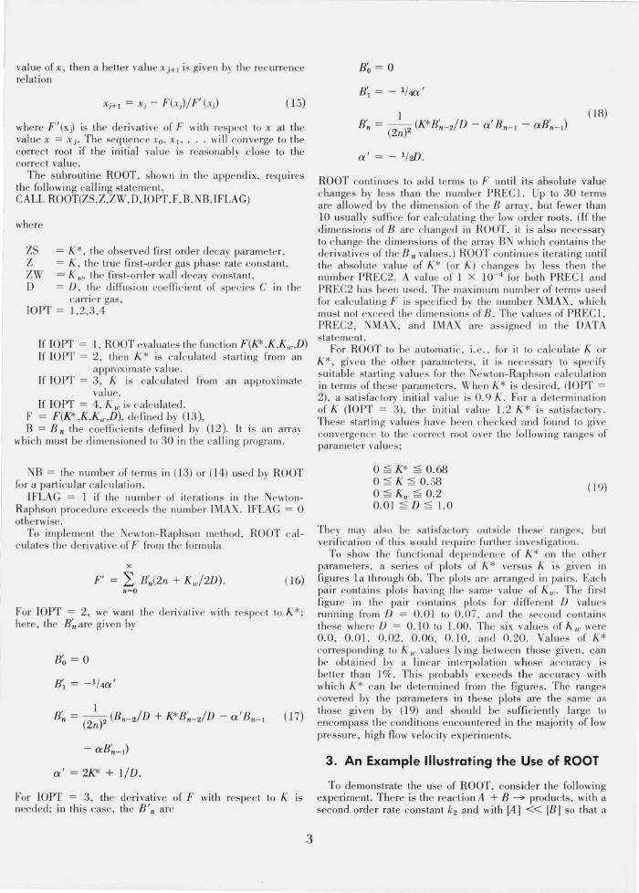
ROOT continues to add terms to F until its absolute value changes by less than the number PREC1. Up to 30 terms are allowed by the dimens ion of the B array, but fewer than 10 usually s uffi ce for calculating the low mder roots . (If the dimens ions of B are changed in ROOT, it is also necessary to change the dimens ions of the array BN wh ich contains the derivat ives of the B n values .) ROOT co ntinues iterating until the absolute value of K* (or K) changes by less then the number PREC2. A value of 1 X 10- 4 for both PRECI and PREC2 has been used. The maximum number of te rms used for calc ulating F is spec ified by the number NMAX, whi ch must not exceed the dimensions of B. The values of PRECl , PREC2, NMAX. and IMAX are assigned in the DATA statement.
For ROOT to be automatic, i.e., for it to calculate K or K* , given th e othe r paramete rs, it is necessa ry to spec ify su itable starting values for the Newton-Raphson cal culation in te rms of these paramete rs. When K* is desired, (IOPT = 2), a sati sfac tory initial value is 0 .9 K. For a dete rmination of K (lOPT = 3), the ini tial value 1.2 K* is sati sfactory. These starting values have been chec ked and found to give co nverge nce to the correc t root over the followin g ranges of parame te r values;
o ~ K* ~ 0.68 0 ~ K ~ 0. 58 o ~ Kw ~ 0.2 O.OJ ~ D ~ 1.0
(19)
They may also be sati sfac tory outs ide these ranges, but verification of thi s would req uire furth er investigation.
To s how the fun ctional de pendence of K* on the other paramete rs, a series of plots of K* vers us K is give n in figures la through 6b. The plots are arranged in pairs. Each pair contains plots having the same value of Kw. The firs t figure in the pair co ntains plots for different D values running from D = 0.01 to 0.07 , and the second co ntains these where D = 0 . 10 to 1.00. The s ix values of K w were 0.0, 0 .01 , 0 .02, 0.06, 0.10, and 0.20. Values of K* correspondin g to Kw values lying be tween those given, can be obtained by a linear inte rpolation whose accuracy is beller than 1%. Thi s probably exceeds th e accuracy with which K* can be determined from the figures. The ranges covered by the parameters in these plots are the same as those given by (19) and should be suffi ciently large to encompass the cond itions encoun tered in the majority of low pressure, high f10w velocity experiments.
3. An Example Illustrating the Use of ROOT
To demonstrate the use of ROOT, consider the following experiment. There is the reaction A + B -7 products, with a second order rate constant k2 and with [A] « [B ] so that a

L
first order rat e constant k = k2 [B] can be defin ed. The reactants are conta ined in a carrier gas flowing through a 2 cm I.D . tube wi th an average linear velocity of 200 cm/s. The measurement of the concentration of A is begun 5 cm downstream from its injection point and is found at 20 cm to have decayed exponentially to 0.1 of its value at 5 cm. When species B is removed from the carri er, A is observed at 20 cm to have decayed to 0.3 of its value at 5 cm. Since A decays in the absence of B, it is assumed to be und ergo ing a first order wall reaction. Thus, k* (total) = 30.7 S - I , and k* (wall) = 16.05 S - I. If the diffusion coefficient of A in the carri er gas at the prevai ling pressure is 20 cm2 S - I , then the values of the dimensionless parameters used by ROOT are, K* (total) = 0.1535, K* (wall) = 0.0803, and D = 0.05.
The first task is to use ROOT to determine K w from the value of K* observed in the absence of B. The following calling program will acco mpli sh thi s.
PROGRAM CALL DIME NSION B(30) ZS = 0.0803 Z = 0.0 D = 0.05 IOYI' = 4 CALL ROOT(ZS,Z,ZW,D, IOPT,F ,B,NB,IFLAG) PRINT ZW END
In this case ROOT wi ll return a value of 0.05 for ZW (=Kw)'
To determine K from K* (total) , use K w = 0.05, and use 1.2 K* = 0.1842 as an approximate vallle of K. Then use ROOT with IOPT = 3 to determine the correct value of K.
0.60
Kw = 0.0 ° 0.07
~ ~ ~ ~ /' 0.01
~ Y /'
~ ,/
0.40
KlIi
~ ~ V
.#. ~ ~ V
0.20
~ :;r
/ V la)
o o 0.20 040 0.60
F IGURE lao Plots oj K* versus KJor D = 0.01, 0.02, 0.03, 0.04, 0.05, 0.06,0.07.
K. ~ 0.0.
The following program accomplishes this.
PROGRAM CALL DIMENSION B(30) ZS = 0.1535 Z = 1.2*ZS (approximate value) ZW = 0.05 D = 0.05 IOPT = 3 CALL ROOT(ZS,Z,ZW,D,IOPT,F, 8 ,NB, IFLAG) PRINT Z END
For this example, ROOT gives 0.0842 for the accurate value ofK.
From these results . the values, k = 16.84 S- I, and kw = 10.00 c m S - I are obta ined for the laboratolY parameters.
It has been assumed in this experimen t tha t the reac tan ts are well mixed 5 cm downstream from the injec tion point of A. This is equivalent to assum ing that only the lead ing term in (8) is being observed. ROOT can be used to determine the higher order decay parameters in (8) . To do this for the above example, the values K = 0.0842, K w = O. OS , a nd D = 0.05 are used with rOPT = 1 to calculate F as a fun ction of K*. From thi s the zero crossing points which correspond to higher roots of (13) can be located and used with IOPT = 2 to get acc urate values. For the present example, the next decay parameter is K~ = 1.3144, which yields k~ = 263 S- I . Therefore, a t 5 c m downstream from the mixing point , the second term in (8) would have decayed to 0.0014 of its I
initial value. Thi s observation does not guarantee that only the lead ing term in (8) is being observed. If the coefficient A2 were much larger than A I then the second term in (8)
0.60
Kw 0.0 001
/. / ~ ~ ~
~ ~ ~ ~ 0.40
~ ~ ~ §:? :;;.---- 10
A ~ ~ ~ 0.20 ~~
/ / (b)
° ° 0.20 0.40 0.60 K
f IGURE lb. Plots oj K* versus KJor D = 0.1, 0.2, 0.3, 0.4, 0.5, 0.6, 0.7, 0.8, 0.9, 1.0.
K .~ 0.0.
4
--- - --- ----
0.60
D -Kw = 0.01
~ 0 .07
~ ~ /' ~ V ../
0.01
A. (3 /" V ./
0.40
~ ~ / A V ../ V
~ V ~ /"
0.20
~ V
V 101 o
o 0.20 040 0.60
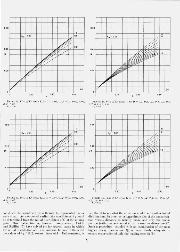
FIG URE 2a. Plols oj K* versus KJor D = 0.01 , 0.02, 0.03 , 0.04 , 0.05 , 0.06,0.07.
K •. = 0.01.
0.60
0 t--Kw = 0.02 Ld
0.07
~ r;: A ~ V ../
0.01
~ ~ V V ./
0.40
~ ~ V ~ ~ V
~ V ~e ,/
0.20
~ ~ L-V ~
101 o
o 0.20 0.40 0.60
FIGURE 3a. Plots oj K* versus KJor D = 0 .01 , 0 .02, 0 .03, 0.04, 0 .05, 0.06,0.07.
K .. = 0.02.
could still be s ignificant even though its exponential factor were small. As mentioned earlier, the coeffic ients A i could be de termined from the radial distriubtion of C at the mixing point. This distriubtion is, however, rarely known. Pirkle and Sigi llito [7] have solved (4) for several cases in which the initial distribution of C was uniform. In none of them did the values of Ai, i ~ 2, exceed those of A l' Unfortunately , it
5
I--
I Kw 0.01 ./ 1 0 '
~ ~ .40 ~ ~ ~
L ~ ~ ~ ~ 1.0
~ ~ ~ ~ ~ IA ~ ~ V
)Ir ~ .20
V V lei
0 o 0.20 K 0.40 0.60
FIGU RE 2b. Plots oj K* versus KJor D = 0. 1, 0 .2 , 0.3, 0.4, 0.5, 0.6, 0.7,0.8, 0.9, 1. 0.
K .. = 0.01.
. ~n
0
Kw k::: 0.1
~ t2 .40 /.. ~ ~ ~.
~ ~ ~ ~ ~ 1.0
~ ~ ~ ~ V
~ ~ ~ p-
.20 ;)It ~ ~
/ ~
Ibl 0
0.20 040 0.60
FIGURE 3b. Plots oj K* versus Kfor D = 0.1 , 0.2 , 0.3, 0.4, 0.5, 0.6, 0.7, 0.8, 0.9, J .0.
K .. = 0.02.
is difficult to say what the si tuation would be for other initial distributions. In practice , a logarithmic plot of the concentration versus distance is usually made and only the linear portion (within experimental error) is used to determine k*. Such a procedure, coupled with an examination of the next higher decay parameters Iq is most likely adequate to ensure observation of only the leading term in (8).

,-
0.60 0 - -h 0.07
Kw = 0.0 ~ ~ ~ V V
A-~ V; V /' 0.01
A ~ V /,V 0.40
~ ~ v V f3 Y /' v
~ ~ /' / A ~ /
0.20
~ ~ V r;/
13)
o o 0.20 0.40 0.60
K
F IGURE 4a. Plols oj K* versus KJor D = 0.01, 0.02, 0.03, 0.04, 0.05, 0.06, 0.07.
K, ~ 0.06
0.60 0
,;; 0.07
Kw = 0.1 ~ ~ /' /'
d: /:: V' V h ~ ~ ./'V V
/' 0.01
d-~ V V/ ./'
V 0.40
~ ~ / V /
~ v:: V / V
A-~ ~ V V /'
A ~ /' / 0.20
~ /'/' V
/ 13)
o o 0.20 0.40 0.60
FIGURE 5a. Plots oj K* versus KJor D = O.OJ, 0 .02, 0.03, 0.04, 0.05, 0.06, 0.07.
K . ~ 0.10.
------
0.60 0 -
/' 0.1
Kw = 0.06 ~ ~ ~ ~ ~ C
~ ~ ~ ~ k:: V
~ ~ ~ ~ ~ r:--- 1.0 0.40
~ ~ ~ ~ A ~ ~ ~
~ p
0.20
~
Ib) o
o 0.20 0.40 0.60
FIGU RE 4b. Plots oj K* versus K (or D = 0. 1, 0.2, 0.3 , 0.4 , 0 .5, 0.6, 0.7, O.B, 0.9, 1.0.
K ,,~ 0.06.
0
0.60 0.1
fl :;:/
-'
Kw = 0.1 ~ V /
/ ~ t::::: ~ ~ ~ ~ ~ ~ ~ :;::: 1.0
~ ~ ~ t§: ~ 0.40
-d ~ ~ ~ ::/'"
~ ~ ~ p-
0.20 ~~
Ib) o
o 0.20 K 0.40 0.60
F IGURE 5b. Plots of K* versus Kfor D = 0 .1 , 0.2 , 0.3 , 0.4, 0.5, 0.6 , 0.7, O.B, 0.9, J .0.
K . ~ 0.10.
6
0
0 .60 :;; 0.07
./-~ ~ Kw = 0.2 ~ :/: :/ /
~ 0 ;/ ./' ./ /
~ /; '/ :/ :/ /' 0.01
/. ~ ~ / /' ./'
/' ./'
0.40
W ~ v V / :/
~ r:/ v L V :/
t% V v V /' V
~ v V V / 0.20
V / V
V (al
o o 0.20 0.40 0.60
K
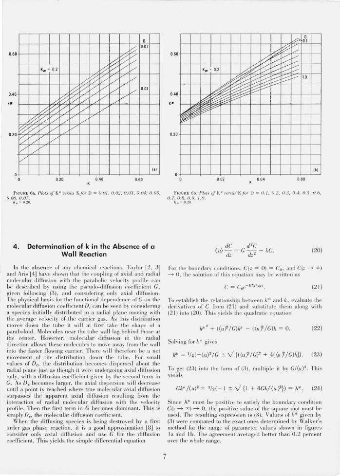
FICURE 6a. Plol.s oj K* versus KJur D = 0.0 / , 0.02, 0.03, 0 .04 , 0 .05 , 0.06, 0.07.
K . = 0. 20.
4. Determination of k in the Absence of a Wall Reaction
In th e absen ce of a ny c he mi ca l reac tions, Tay lor [2, 31 and Aris [4] have s hown th at the couplin g of axial and rad ia l molec ular diffus ion with the paraboli c ve loc ity profi le can be described by using th e pse udo-diffus ion coe ffi c ie nt C , given following (3), and conside ring only ax ial diffus ion. The physical basis for the fun ctional de pe nde nce of C on the molec ular d iffus ion coeffi c ie nt Dc can be seen by cons iderin g a s pec ies initially di s tributed in a rad ial plane moving with the average veloc ity of the carrie r gas. As thi s di s tributi on moves down the tube it will a t first ta ke the shape of a paraboloid. Molecules near th e tube wall lag be hind those at the ce nte r. However, mol ec ul ar diffusion in the radial direction allows th ese mol ec ules to move away from the wall into the faster flowing ca rrie r. T here wi ll the re fore be a net move ment of the dis tribution down th e tube. For s mall values of Dc> the dis tribution beco mes d ispersed abou t the radial plane just as though it were und e rgo ing ax ia l diffu s ion only, with a diffusion coeffi c ie nt give n by the seco nd term in C. As Dc becomes larger , the ax ial di spe rsion will decrease until a point is reac hed where true mol ec ul a r ax ia l d iffu s ion su rpasses the apparent axial diffusion resulting from the intel'action of radial molec ular diffus ion with the veloci ty profile. Then the firs t term in C becomes dominant. Thi s is simpl y Dc, the molec ular diffusion coeffi cien t.
When the diffus ing species is being destroyed by a first order gas phase reac tion , it is a good approximation [8] to co ns ide r only axial diffusion and use C for the diffus ion coeffi c ient. This yields the simple differe ntial equatio n
7
~. 0
0.1
0.60 ~ ./
~ ,./
~ ~ ~ -:::: Kw = 0.2 ~ ~ ::::::: V ~ :::::
h~ % ::;::: ::::--::: k ~ :::..--- 1.0 :::-.-:::
lA ~ ~ ~ ~ -:;:/
~ ~ ~ p ---0.40
A ~ ~ ~ ~ ~
0.20
(bl o
o 0.02 K 0.04 0.60
FI GU R E 6b. Plo/.., q( K* lIersus KJor D = 0./ , 0.2. 0.3, 0.4, 0.5, 0.6, 0.7,0 .8, 0.9, /. 0.
K . = 0.20.
dC d 2C ( u) - = C - - kC.
dz dz 2 (20)
For the boundary co nditions, C(z = 0) = Co, a nd C(z ~ 00) ~ 0 , the so lution of thi s equation may be wrillen as
(21)
To establi sh the rela ti onshi p between k* and k, evalua te the derivatives of C from (2 1.) and subs titute the m along with (21) into (20). Thi s yields the quadra ti c equation
k*2 + ((u'f/CW - ((u1!C)k = 0. (22)
Solving fo r k* gives
k* = Ih(-(U)2/C ± V {((u'f/C)2 + 4((u';C)k}). (23)
To ge t (23) into th e form of (3), multiple it by C/(U)2. Thi s yie lds
Ck* /( U)2 = th( -1 ± V {I + 4Ck/ (u )2}) = A*. (24)
Since A* must be pos itive to sati sfy the boundary condition C(z ~ 00) ~ 0, the pos itive value of the square root must be used. The resulting expression is (3). Values of k* given by (3) were compared to th e exac t ones determined by Walker's method for the range of parameter values s hown in figures l a and lb. The agreement ave raged beller than 0.2 percent over the whole range.
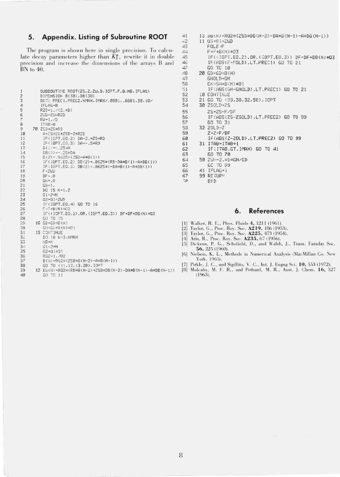
5. Appendix. Listing of Subroutine ROOT
The program is s hown here in single prec ision. To cal c ulate decay parameters higher than K~, rewrite it in doubl e precision and inc rease the dimensions of the arrays Band BN to 40.
I SUSgOUTI NE ROOTCZS.Z.ZW.D. IOPT.F.B.NB. IFLAG ) 2 DI ME NSIoti B(30).DBC30l 3 D~, TC, PREC1.PREC2.NMAX.IMAX/.0013i •. 08131.313. \£l/ 4 lFLAG=0 5 R2D-I./C2.*D) b ZI.JD-Zl,h'R2D 7 RD-!,/D 8 lTH8=fl 9 70 ZSD=ZS,"RD 10 A = <~:3*ZS +ZSD-Z*R2D 11 IF (IC PT . EO . 2) DA~2.*ZS+RD 12 iF ': ;OPT.[O.3) DA=- .5*RD 13 B( I) =-' .25*A 14 D8 C1.l=- . 25'1,J:,A 15 B(2)= . 9625*( ZSD -A>I<B (I)) 16 iFCiOPT.EO.2) DS (2)= . 0525*CRD-DA*8C I)-A*D8(1)) 17 IF ( lO?T.EQ.3 ) D8(2)=.0625*(-DA*BCll-A*D8(\)) 18 F=Z lJD 19 DF=.1'i 20 GH= .8 21 GD-!. 22 DO 15 N=L2 23 QI=2*N 24 Q2 =Q I '·ZlJD 25 Ic (IDPT .EQ . 4 ) GO TO 16 26 27 28 29 30 31 32 33
35 36 37 38 39 413
r ",'+8 ( N) 'KQ2 II' ( !cPT . EO. 2) .OR. C IOPT . EO .3)) DF=DF+DBCN)*02 GO TO ~5
16 GD-GD+8(H ) Gti=GI; +8 (N) "'0 1
15 C1H-'- lN0E DO 10 h~3.NMAX N8=I'j
02=Ql*!J~ RQ2:: 1. /Q2 8 CH) 'RQ2"< (Z5D*8 (N-2) -A '"B ( fl-l)) GO TO (1 L 12. 13,2(3). IOPT
12 DS (N; -RQ2,,(RD*8 (N-2) +ZSD"'DB CN -2 ) -DA>I<B (N-I) -R*D8 (N-I )) GO TO 11
41 ~2 43 44 45 4i; 47 48 49 50 '; 1 52 53 54 55 56 57 53 59 60 61 62 63 64 65 66 f'i7 ~p
13 V~lN)-RQ2*(ZSD*DB(N-2)-DA*B(N-l)-A*D8CN-l)) 11 Q,\-O i +ZUD
FOLD "P F·F +B<r~) *03 IF((IGPT .EQ. 2).OR . (iOPT .EQ.3)) DF-DF+DBCN1*Q3 IF CABS(F-FOLD).LT. PREC1) GO TO 21 GO TO 10
213 GD-GD+BCNI GHOLD-GN G~; -GH+8 ( ~l ) *Q 1 IF (ABS( GN- GNOLD).LT.PREC1) GO TO 21
, 0 CONTlH~E 21 GO TO (:39.30.32,50 I , IOPT 30 2S0LD:::2S
ZS-ZS-F/DF IF (~BS(ZS-ZSOLD).LT.PREC2) GO TO 99 GO TO 31
32 ZOLD"Z Z-Z-F/DF IF(HBS(Z-ZOLD).LT.PREC2) GO TO 99
31 !TAB - !TAB+ 1 IF ( !TAB. GT. IMAX) GO TO 41 GO TO 70
50 ZU--·2. ,,'D*G N/GD GO TO 99
41 IFU1G-j 99 RE ,-U",I~
E~~D
6. References
[IJ Walker, R. E., Phys . Fluids 4,1211 (1961). [2] Tay lor, G., Proc. Roy. Soc. A219, 186 (1953) . [.3] Tay lor, G. , Proc. Roy. Soc. A225, 473 (1954). [4] Ari s, R. , Proc. Roy. Soc. A235, 67 (J956). [5] Dickens, P. G. , Schofield, D. , alld Walsh, J. , TrailS. Faraday Soc.
56, 225 (1960). r6] Nielson , K. L. , Methods in Nume ri cal Anal ysis (MacMillan Co. New
York , 1965). [7] Pirkle, 1. C, and Sigillito. V. C . lnt. J. Engng Sci. 10, 553 (1972). [8] Mu lcahy, M. F. R .. and Pet hard , M. R. , AusL 1. Chem. 16, 527
(1963).
8


