
1
Transpiration of Eucalyptus woodlands across a natural gradient 1
of depth-to-groundwater 2
SEPIDEH ZOLFAGHARA,B
, RANDOL VILLALOBOS-VEGAA,B
, MELANIE ZEPPELC, 3
JAMES CLEVERLYA, RIZWANA RUMMAN
A,B, MATTHEW HINGEE
A, NICOLAS 4
BOULAINA, ZHENG LI
A, DEREK EAMUS
A,B 5
6
A School of Life Sciences, University of Technology Sydney, PO Box 123, Broadway, 7
Sydney, NSW, 2007, Australia 8
B National Centre for Groundwater Research and Training, University of Technology 9
Sydney, Australia 10
C Department of Biological Sciences, Macquarie University, Balaclava road, North Ryde, 11
NSW, 2107, Australia 12
13
Corresponding author: SEPIDEH ZOLFAGHAR 14
Email: [email protected] 15
16
17
Running head: Impact of groundwater depth on transpiration 18
19

2
Abstract 1
Water resources and their management present social, economic and environmental 2
challenges, with demand for human consumptive, industrial and environmental uses 3
increasing globally. However environmental water requirements, that is, the allocation of 4
water to the maintenance of ecosystem health, are often neglected or poorly quantified. 5
Further, transpiration by trees is commonly a major determinant of the hydrological balance 6
of woodlands but recognition of the role of groundwater in hydrological balances of 7
woodlands remains inadequate, particularly in mesic climates. 8
In this study we measured rates of tree water use and sapwood 13
C discrimination in a 9
mesic, temperate Eucalypt woodland along a naturally-occurring gradient of depth-to-10
groundwater (DGW), to examine daily, seasonal and annual patterns of transpiration. We 11
found that: 12
a) the maximum rate of stand transpiration was observed at the second shallowest site 13
(4.3 m) rather than the shallowest (2.4 m); 14
b) as DGW increased from 4.3 m to 37.5 m, stand transpiration declined; 15
c) the smallest rate of stand transpiration was observed at the deepest (37.5 m) site; 16
d) there was a strong (r2 = 0.98) negative linear correlation between average monthly 17
stand transpiration and the δ13
C of current year’s sapwood, indicative of increasing 18
water-use-efficiency with decreasing availability of groundwater; and 19
e) there was no evidence of convergence in rates of water use for co-occurring species at 20
any site. 21

3
We conclude that even in mesic environments groundwater can be utilised by trees. We 1
further conclude that these forests are facultatively groundwater dependent when 2
groundwater depth is < 9 m and suggest that during drier-than-average years the 3
contribution of groundwater to stand transpiration is likely to increase significantly at the 4
two shallowest groundwater sites. 5
Key words: Groundwater depth; tree water-use; transpiration; groundwater 6
dependent ecosystems; 13
C stable isotopes 7
8

4
1. Introduction 1
Demand for freshwater is increasing globally in line with increasing population size, 2
with water being required especially for human consumptive use, irrigation and other 3
industrial applications (Gleick et al., 2006). To manage limited fresh water resources 4
sustainably, demand by all sectors (e.g., environmental, municipal, agricultural; Cleverly et 5
al. 2002)) needs to be quantified and managed (Cleverly et al., 2002). However, 6
environmental water requirements have traditionally received little attention and are often 7
neglected or underestimated (Eamus et al. 2005). Allocation of water to the environment has 8
frequently been limited to an allocation of water to ensure river flows (Murray et al. 2003). It 9
is now understood, though, that environmental water requirements should include allocations 10
to wetlands, woodlands, mound springs and a myriad of ecosystems that require groundwater 11
to maintain their current structure and function (Eamus et al. 2006b). 12
Transpiration by trees can be the major pathway for discharge of water from 13
woodlands and consequently determines the hydrological balance of woodlands, exceeding 14
transpiration by grasses and shrubs (Dragoni et al. 2009; Eamus et al. 2006b; Zeppel and 15
Eamus 2008). Spatial and temporal variation in tree water-use and differences among species 16
can be explained by variation in micro-climate, and species-specific physiological and 17
structural properties, including rooting depth, hydraulic architecture, leaf area and tree size 18
(O'Grady et al. 2007; Rossatto et al. 2012; White et al. 2002; Zeppel and Eamus 2008). 19
Trees have access to two or three sources of water: a) recent rainfall in the upper soil 20
profile; b) water deeper in the profile from past rainfall events; and in some locations, c) 21
groundwater and its associated capillary fringe (Eamus et al. 2006b; Naumburg et al. 2005). 22

5
Access to groundwater can affect plant growth, survival, rate of water-use and local water 1
budgets (Carter and White 2009; Miller et al. 2010; Zencich et al. 2002). In semi-arid 2
Western Australia, for example, increased depth to the shallow, unconfined Gnangara aquifer 3
over the past several decades has resulted in floristic changes including widespread mortality 4
of native woodlands (Groom et al., 2000; Canham et al., 2009; Stock et al., 2012). However 5
detailed assessment of seasonal and inter-annual variability in tree water-use at sites with 6
differential access to groundwater has not been made for this or any other important 7
municipal water source in Australia. This is in contrast to numerous studies quantifying 8
water use in riparian forests of semi-arid south-western America (Cleverly et al., 2002; Scott 9
et al., 2004; Nagler et al., 2005). In fact groundwater use by trees growing over shallow water 10
tables is extensive across arid and semi-arid regions (Cleverly et al. 2006; Scott et al. 2006; 11
Smith et al. 1998). Where groundwater-use has been identified and quantified, differences in 12
rates of stand water-use can be explained by differences in groundwater availability, which 13
can be inferred from groundwater depth (Baird et al. 2005; Carter and White 2009; O'Grady 14
et al. 2007). 15
Generally it is assumed that transpiration decreases monotonically with increasing 16
depth-to-groundwater (DGW) (Butler et al. 2007; Landmeyer 2012; McDonald and Harbaugh 17
1988). However, it is more likely that transpiration is maximised at an optimal DGW that 18
varies by plant functional type and rooting depth (Baird et al. 2005; O'Grady et al. 2011; 19
Zeppel 2013), but this has rarely been tested in the field. While there is little question that 20
transpiration is smallest where groundwater is deepest (Carter and White 2009), counter-21
intuitive reductions in transpiration rates as groundwater becomes shallower than the optimal 22
depth may arise from anoxia in the root zone. Altogether, groundwater-use by trees is 23
dictated by DGW, plant functional type, and climate variability, and this results in variation 24
in the timing and amount of groundwater dependence (Eamus et al. 2006a) at any given site. 25

6
In contrast to the many studies undertaken in arid and semi-arid regions, few have 1
compared rates of tree water-use along a naturally occurring gradient of DGW in mesic 2
regions (Carter and White 2009; Gazal et al. 2006; Lamontagne et al. 2005). Consequently 3
we examined spatial and temporal patterns of transpiration in a mesic, temperate Eucalypt 4
woodland across a naturally occurring gradient in DGW. Groundwater-use by vegetation at 5
these same sites has been established through multiple data sets, including step changes in 6
structural attributes (e.g. basal area, leaf area index and tree height; Zolfaghar et al., 2014), 7
hydraulic architecture and water relations (Zolfaghar et al., 2015a, b). A single, normalised 8
response function using 16 multiple-scale (leaf, branch, tree, stand) traits has been developed 9
for this site which describes the impact of differences in groundwater depth on ecosystem 10
structure and function (Eamus et al., 2015). 11
Our objectives in the current study were to: 12
1) Quantify spatial and temporal patterns in rates of stand water-use at multiple sites differing 13
in DGW; 14
2) Determine whether variation in intra-specific stand water-use can be explained by 15
variation in DGW; 16
3) Determine whether variation in 13
C:12
C ratios of stem wood can provide insight to 17
variation in water-use-efficiency across sites differing in DGW; 18
4) Determine whether, during relatively dry periods, rates of transpiration will decline more 19
at the deepest DGW sites than at shallower sites; and, 20
5) Compare rates of tree water use for co-occurring species at a number of sites, to establish 21
whether convergence to a common rate of water use is apparent. 22

7
2. Material and Methods 1
2.1. Site description 2
This study reports on a detailed assessment of daily and seasonal transpiration over 16 3
months at four sites located across an 8.5 km transect in remnant native Eucalyptus woodland 4
within the Kangaloon bore-field of the Upper Nepean catchment; 110 km south-west of 5
Sydney, New South Wales, Australia (between 34o29’ S 150
o34’ E and 34
o32’ S 150
o37’ E). 6
These four sites were chosen to span a range of average DGW (2.4 m, 4.3 m, 9.8 m and 37.5 7
m) within the same climate regime (Fig. 1). DGW in this area has been monitored by the 8
Sydney Catchment Authority (SCA) on a daily basis since 2006. Each experimental site was 9
centred around a single groundwater monitoring bore, with all measurements of sapflow and 10
leaf area index (LAI) conducted within 50 m of this bore. During the drought period 2006 – 11
2010 inclusive, DGW was typically 1-3 % deeper at the deepest site (37.5 m DGW) 12
compared to the study period of 2011-2012. However for the remaining three shallower sites, 13
DGW was 8 to 37 % deeper during the drought years than during the two wet years of this 14
study. Nevertheless average DGW fluctuated minimally (<10%) across all sites for the period 15
2006 – 2012. 16
The study area receives a long-term average annual rainfall of 1067 mm 17
(http://www.bom.gov.au 2000-2010). On average February is the wettest month (186 mm), 18
while August is the driest month (51 mm). Average (2000-2012) minimal and maximal 19
temperatures occur in July (2.7 oC) and January (24.3
oC), respectively. During the study 20
period (2011–2012), reference evapotranspiration (ET0) was estimated using the Penman-21
Monteith method (Allen et al. 1998). ET0 was parameterised with local meteorological 22

8
measurements of daily net radiation (NRLite, Kipp and Zonen, Delft, The Netherlands), 1
vapour pressure deficit (VPD; HMP45C, Vaisala, Helsinki, Finland), LAI and wind speed 2
(wind sentry 03001, R.M. Young Company, MI, USA) at two metres height. 3
The dominant tree species were defined during field surveys of basal area as those 4
that, when summed, accounted for > 80% of total standing tree basal area. Overall there were 5
five dominant Eucalyptus species across four sites: E. radiata, E. piperita, E. globoidea, E. 6
sieberi and E. sclerophylla (Table 1). Each site contained 2–3 dominant tree species. 7
Structural characteristic of all four sites are presented in Table 2. 8
2.2.Soil moisture measurements 9
Volumetric soil moisture content was measured with -1 which were installed in all four sites 10
that were instrumented with sapflow sensors (see below). These probes were buried 11
horizontally at depths of 10 cm, 30 cm and 50 cm in sites having 2.4 m and 4.3 m DGW and 12
at 10 cm and 30 cm in sites having 9.8 m and 37.5 m DGW. Limited numbers of sensors were 13
available and hence there we no sensors at 50 cm in the two deeper groundwater sites (9.8 m 14
and 37.5 m DGW). 15
2.3. Sapflow measurements 16
At each site, 10 healthy trees across two or three dominant species (Table 1) were 17
instrumented with sapflow sensors (see below) to determine whole-tree rates of water-use. 18
Trees were selected across a representative range of DBH (Diameter at Breast Height) to 19
allow scaling from individual to stand scales. Measurements commenced in January 2010 20
(summer) at the 37.5 m DGW site and continued until December 2012 (summer). Sensors 21
were installed at the three remaining sites between mid-2010 and September 2011 such that 22
9
sapflow was measured concurrently at all four sites for a 16-month period (Sept 2011–Dec 1
2012 inclusively). 2
Heat dissipation sapflow sensors (Granier 1985) were used to measure rates of tree 3
water-use. Sensors were manufactured in the laboratory of the terrestrial ecohydrology 4
research group (TERG) at the University of Technology Sydney (UTS). Three independent 5
laboratory calibrations of these sensors against transpiration rates measured in weighing 6
lysimeters were conducted and confirmed that the estimates of sapflow velocity were within 7
the accepted range of accuracy (Zolfaghar 2014). 8
Two probes were inserted radially into the stem sapwood with a vertical separation of 9
a minimum of 10 cm, wherein the upper probe was located at 1.3 m height. The upper probe 10
contained a thermocouple and electric heater that was provided with constant power (0.2 W), 11
while the lower probe contained only a thermocouple. The two temperature (T) sensors 12
measure heat dissipation from sapwood and xylem water, which increases as a function of 13
sapflow. This approach enables the measurement of xylem sapflow velocity from the 14
relationship between difference in temperature and sap velocity. When sapflow velocity is 15
zero, the temperature difference between the two sensors is maximal. Granier (1985) defined 16
a flow index (K); calculated from the measured temperature difference between the upper 17
heated sensor and the lower reference sensor (∆T) and the maximum measured temperature 18
difference, occurring at zero flow velocity (∆Tmax): 19
𝐾 =(∆𝑇𝑚𝑎𝑥−∆𝑇)
∆𝑇𝑚𝑎𝑥 Eq. (1) 20
The value of ∆T is determined from the differential voltage measured between the 21
upper and lower thermocouple. The following empirical relation between the value of K and 22
the actual sapflow velocity (V) was found (Equation 2; (Lu et al. 2004): 23
10
𝑉 = 0.0119 × 𝐾1.231 𝑐𝑚/𝑠 Eq. (2) 1
In the current study, at least one additional 3-probe sensor was used in each tree. 2
Three probes systems record the natural temperature gradient in the sapwood, which is then 3
subtracted from the measured ∆T. The third probe was located at the same height as the 4
heated probe, which was equidistant to both reference probes (i.e., 10 cm laterally and 5
longitudinally). During the life of the project the sap flow sensors were inspected on monthly 6
basis and in average every three months (could be longer or shorter according to the 7
condition of the sensors) were replaced. 8
2.4. Zero flow 9
To calculate K, ∆Tmax was determined for discrete seven-day intervals during the 10
study period using a double regression method (Lu et al. 2004). Having established ∆Tmax 11
every seven days, K was calculated for each tree using Equation 1. Sap velocity was 12
calculated using Equation 2 for each sensor (m s-1
). Temperature differences between sensors 13
were measured once per minute and recorded as 10-minute averages. 14
2.5. Sapwood area 15
At each site, sapwood cross-sectional area (SA) across a range of tree sizes in each 16
species was determined on samples that were collected using a six millimetre diameter 17
increment corer. Two perpendicular cores were taken from each tree (8-10 trees were 18
sampled from each species). Sapwood was distinguished from heartwood by visual inspection 19
of a distinct colour change. When the boundary between sapwood and heartwood was not 20
clear, sapwood was stained with Methyl orange. Sapwood depth was used to calculate SA by 21
assuming a circular cross-section. Estimating SA was critical for scaling flow rates to whole 22
tree and stand scales. 23

11
2.6. Spatial scaling 1
To scale transpiration rates from individual trees to the entire stand, DBH of all trees 2
within three replicate plots (20 m × 20 m) was measured at each site, from which the total 3
sapwood area per hectare of land was estimated for each species (SAspecies). The average sap 4
velocity of each species in each hour (SVspecies) was multiplied by SAspecies to determine 5
sapflux (Js) (Zeppel et al. 2008): 6
𝐽𝑆 = ∑ 𝑆𝐴𝑠𝑝𝑒𝑐𝑖𝑒𝑠 × 𝑆𝑉𝑠𝑝𝑒𝑐𝑖𝑒𝑠 Eq. (3) 7
In each 24-hour period, 10-minute Js was summed to determine daily sapflow rates, 8
expressed as a volume (cm3 day
-1) (Zeppel et al. 2006) and scaled by ground area (mm day
-1). 9
In those species that were not used for measurements of sapflow and which accounted for 10
less than 20% of the tree basal area of each site, Js was estimated as the product of average 11
velocity of all trees measured at the site (SVsite) and SAspecies. At each site, daily rates of stand 12
transpiration in each tree species were calculated by summing Js, expressed as volume of 13
water transpired per unit ground area per day (mm day-1
). Stand transpiration was calculated 14
by summing the daily transpiration of all species at a site. 15
2.7. Stable isotope analysis 16
Tree cores (one core per tree) were collected from each of the sites with a power corer 17
at slow speed. The cores were polished with sandpaper but no distinctive tree rings were 18
observed. Due to the lack of distinctive tree rings to identify annual growth increments, slices 19
were collected from the core every 300 µm with a microtome. A total of 20-25 samples were 20
collected from the sample year sapwood of each core (i.e., a roughly six mm outer segment of 21
the core, beginning below the bark and vascular cambium). Samples were finely ground 22
using a bead mill grinder, and ~100 - 200 mg of sample was transferred into a 3.5 mm X 5 23
12
mm tin capsule. The carbon isotopic composition was measured using a Picarro G2121-i 1
analyser for isotopic CO2. 2
The carbon isotope ratio of plant material (δ13
C) is quantified on parts per thousand 3
basis (i.e., per mil ‰; Equation 4): 4
δ13
C ‰ = (Rsample / Rstandard − 1) × 1000 Eq. (4) 5
6
where R is the 13
C /12
C isotopic ratio relative to the standard reference material (Vienna Pee 7
Dee Belemnite). Intrinsic water use efficiency (WUEi) was calculated from Equation 5: 8
WUEi = [Ca(b-Δ13
C)]/[1.6(b-a)] Eq. (5) 9
10
where a and b are fractionation factors for CO2 arising from discrimination against 13
CO2 11
compared to 12
CO2 during diffusion through stomatal pores (a = 4.4%o) and by the enzyme 12
Rubisco (b = 27 %o). Ca is the concentration of CO2 in the atmosphere and Δ13
C is the 13
discrimination shown by the plant against 13
C arising from both the diffusional and enzymic 14
processes. There is a linear correlation between Δ13
C and WUEi. Δ13
C was calculated from 15
Equation 6: 16
Δ13
C = (-8- δ13
C)/(1+ δ13
C/1000) Eq. (6) 17
18
See Farquhar et al., (1989) for further details. 19
20
2.8. Statistical analysis 21
The differences between SA and DBH of different species and sapflow density of all 22
species within each site for three representative days were tested using analysis of variance 23
(ANOVA). The relationship between DBH and SA and the relationship between sap velocity 24
13
and DBH were also tested using power function regression (Meinzer et al. 2005). Analysis of 1
covariance (ANCOVA) was used to test the null hypotheses that: 1) the regression 2
coefficients were equal to zero amongst all species; and, 2) the slope of the DBH-SA 3
relationship did not differ amongst species. For all statistical tests depth-to-groundwater was 4
considered as independent variable. Analyses were performed using IBM SPSS 5
STATISTICS (version 19, Armonk, NY, USA). 6
3. Results 7
3.1. Climate 8
Total rainfall was 1561 mm in 2011 and 1188 mm in 2012, which were 46% and 11% 9
larger than the long term average (1067 mm yr−1
; 2000–2010). During the 694 days that 10
measurements of sapflow were collected, rainfall was received on 415 days. Mean summer 11
and winter temperatures were 16º and 7oC respectively. Thus the climate of these sites is best 12
described as temperate mesic with warm summers and cool winters. VPD was very low 13
(mean summer and winter VPD were 0.45 and 0.25 kPa, respectively) and generally 14
remained below 1 kPa during the experimental period (Fig. 2). It is apparent that 2011 and 15
2012 were wetter, cooler and more humid than the long-term average values. 16
Soil water content measurements during 2012 showed that the site with deepest water-table 17
(37.5 m DGW) had the lowest soil water content except a short period in early March 2012 18
(Figures shown in Supplementary data). During 2012 measurement, the site with 4.3 m DGW 19
constantly had larger soil water content (maximum of 0.61 g cm-3
). (Figures in supplementary 20
data). 21
22
23

14
Relationships amongst DBH and sapwood area 1
As DBH increased, SA increased in all species and across all sites (Fig. 3). The 2
relationship between SA and DBH at each site varied significantly between species except at 3
the site where DGW was 9.8 m (species × site, F = 1.106; p = 0.35; df = 2,19). Likewise, the 4
coefficient of determination (r2) was different between species within each site except at the 5
deepest site (37.5 m DGW). Additionally, regression coefficients were significantly different 6
across sites for all species. Stem diameter explained 87–97% of variation in SA. 7
Sapflow density 8
The diurnal pattern of sapflow density (cm3 cm
-2 h
-1) on three representative days in 9
summer 2011–2012 (December–February) and winter 2012 (June–August) display typical 10
diurnal patterns with maximum values occurring around noon in both seasons (Fig. 4 and Fig. 11
5). Transpiration rates tended to peak earlier in the day during the summer compared to 12
winter (cf. Figs. 4 and 5). 13
Climatic conditions of the study area during the three representative days that are 14
illustrated in Figures 4 and 5 are presented in Table 3. During both seasons ET0 and VPD 15
were consistently small. Variations in the difference between maximum and minimum 16
temperatures were larger during the summer than in the winter, but conditions were otherwise 17
relatively constant during each representative period. 18
During summer 2012 average sapflow density of the three representative days was 19
larger in the two deepest sites (9.8 m and 37.5 m DGW) than the two shallowest sites. At that 20
time, sapflow density in E. globoidea reached a maximum of 13.75 cm3 cm
-2 h
-1 at site 37.5 21
m DGW but only 8.90 cm3 cm
-2 h
-1 at site 4.3 m DGW (Fig. 4). Similarly, sapflux density in 22
E. piperita was largest at site 9.8 m DGW (Fig. 4). Among the two shallowest sites sapflow 23

15
density reached a higher peak in E. radiata at site 2.4 m DGW than in any of the dominant 1
species at site 4.3 m DGW. Sapflow density was smaller during winter than in the summer 2
because of the cooler temperatures and smaller VPD in winter compared to summer. 3
In summer maximum rates of average sapflow density were similar across species at 4
the 4.3 m DGW site but for the remaining three sites there was variation in maximum rates of 5
sapflow density among species (Fig. 4). Likewise, inter-specific differences in water-use 6
during winter were observed at three sites: 2.4 m DGW (larger diurnal sapflow density in E. 7
radiata), 4.3 m DGW (smaller in E. piperita) and 9.8 m DGW (larger in E. piperita) (Fig. 5). 8
On average and including nocturnal measurements, sapflow density in E. piperita during 9
winter was significantly smaller than for other species at site 4.3 DGW (F=10.76, p<0.001; 10
df=2,213). In contrast at site 9.8 m DGW, sapflow density in E. piperita was significantly 11
larger than in co-occurring species (F=5.58, p=0.004; df=2,213). In the regression analysis 12
between sap velocity and DBH, none of the derived slopes were significantly different from 13
zero (F=0.47, p=0.57; df=1,358), which indicates that there was not a significant effect of tree 14
size on sap velocity. 15
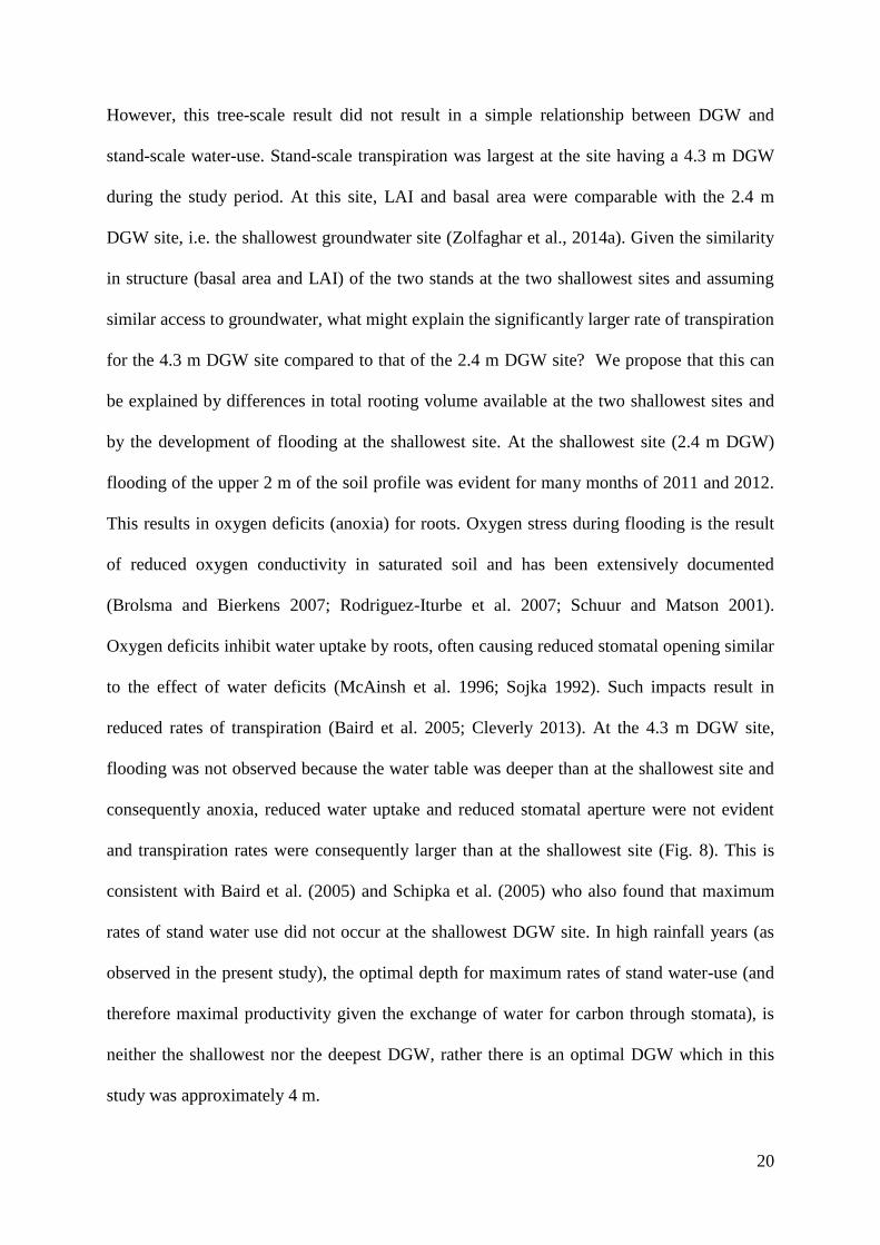
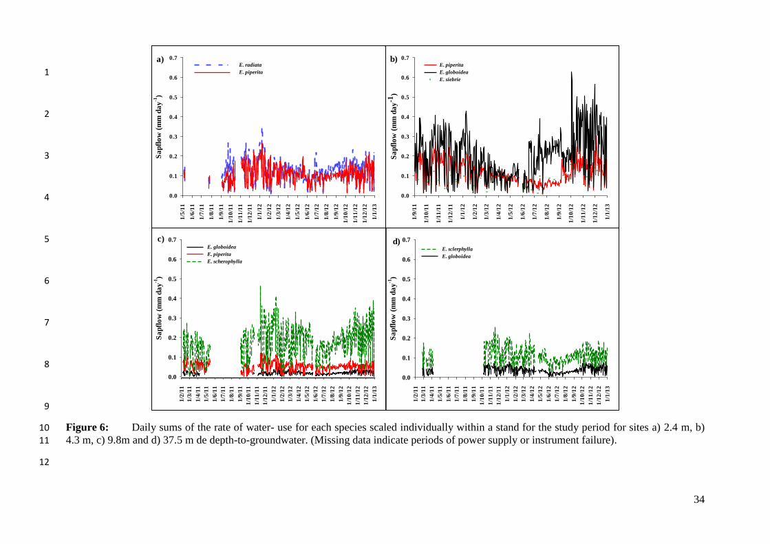
At site 2.4 m DGW, daily transpiration reached a maximum of 0.35 mm day-1
for E. 16
radiata and transpiration rate in E. radiata was consistently larger than in the co-occurring E. 17
piperita (Fig. 6a). Both species exhibited larger maximal daily rates of transpiration in 18
summer than winter because of the longer sunlit period, warmer temperatures and larger daily 19
average VPD in summer than winter (cf. Figs. 2 and 6a). 20
The daily rate of transpiration in E. globoidea growing at the 4.3 m DGW site was 21
larger than that of the other two co-occurring species (maximum 0.62 mm day-1
) across the 22
entire study period (Fig. 6b), and these differences were larger in summer than winter. On 23

16
average the lowest rates of daily transpiration at the site with 4.3 m DGW were recorded for 1
E. sieberi, except during a short period in September 2012 when transpiration in E. sieberi 2
was larger than that of E. piperita (Fig. 6b). 3
E. sclerophylla was dominant at the two sites with deeper groundwater and showed 4
the largest transpiration rates compared to the co-dominant species at these sites. At site 9.8 5
DGW E. sclerophylla transpired a maximum of 0.46 mm day-1
, which was second only to the 6
maximum rate obtained by E. globoidea at site 4.3 DGW (cf. Figs. 6b and 6c). By contrast, E. 7
globoidea maintained the lowest transpiration rates at sites 9.8 m and 37.5 m DGW compared 8
to the other two species at that site (Fig. 6c). At site 37.5 m DGW, E. sclerophylla 9
maintained a larger transpiration rate than E. globoidea throughout the entire measurement 10
period (Fig. 6d). The rate of transpiration of E. sclerophylla at 9.8 m DGW was 11
approximately twice that observed at site 37.5 m DGW (Figs. 6c, 6d). 12
Stand transpiration was calculated by summing the daily transpiration of all species 13
measured at each site (i.e., the sum of all species in each panel of Fig. 6). Throughout most of 14
the period from September 2011 to December 2012, the rate of stand transpiration was largest 15
at the 4.3 m DGW site, where peak summer and winter rates of stand transpiration were 16
approximately 1.35 mm day-1
and 0.80 mm day-1
, respectively (Fig. 7). In contrast, the 17
deepest site (37.5 m DGW) exhibited the smallest rates of stand transpiration across the 16-18
month study period, reaching peak summer and winter rates of 0.57 mm day-1
and 0.30 mm 19
day-1
respectively (Fig. 7). The rates of stand transpiration at sites 2.4 m DGW and 9.8 m 20
DGW were intermediate and overlapped considerably across the 16-month period: peak 21
summer rates were 0.76 mm day-1
(2.4 m DGW) and 0.71 mm day-1
(9.8 m DGW) while 22
winter stand transpiration was 0.42 mm day-1
and 0.37 mm day-1
, respectively. 23

17
Monthly site-level totals of stand transpiration followed a seasonal pattern, with larger 1
rates in summer (5 – 18 mm month-1
) than winter (2.5 – 12 mm month-1
) (Fig. 8). The largest 2
rates of monthly transpiration (e.g., 25 mm month-1
, October 2012) were consistently 3
observed at site 4.3 m DGW, although the difference across sites was smaller during winter. 4
Monthly total stand transpiration for all tree species present (including sub-dominant 5
trees) showed a pronounced peak at 4.3 m DGW, with rates of water-use declining rapidly at 6
deeper and shallower sites (Fig. 8). Inter-monthly variability in monthly stand transpiration 7
was largest at the 4.3 m site and smallest at the deepest groundwater site (37.5 m DGW). 8
Cumulative rainfall and stand transpiration of all tree species (including estimated 9
rates in sub-dominant species) are presented for the year 2012 (Fig. 9). Cumulative rainfall 10
during 2012 was 1188 mm. Total annual stand transpiration was largest at site 4.3 m DGW 11
(188 mm) and smallest at site 37.5 m DGW (95 mm). Between sites, differences in 12
transpiration were small during winter and increased during the dry spring and summer, 13
especially at site 4.3 m DGW where cumulative transpiration was always larger than at the 14
other sites (Fig. 9). 15
The δ13
C increased significantly with increasing DGW (F = 54.17, P < 0.001; Table 16
2). The largest (–27.55) δ13
C were measured at the deepest DGW sites. The smallest δ13
C was 17
recorded at the 4.3 m DGW site. The δ13
C of the shallowest DGW site did not conform to this 18
trend and maintained a δ13
C that was closer to the values recorded at the deepest sites (Table 19
2). 20
The δ13
C of current year sapwood was linearly correlated with average monthly rates of stand 21
transpiration (Fig. 10). The site with the largest rate of monthly transpiration (4.3 m DGW) 22
maintained the most negative δ13
C (and hence the smallest intrinsic water use efficiency; 23

18
WUEi =43 µmol mol-1
) and the site with the smallest rate of monthly transpiration (37.5 m 1
DGW) had the largest (least negative) δ13
C of sapwood (and hence the largest intrinsic water 2
use efficiency; WUEi = 73.4 µmol mol-1
). Intrinsic water use efficiency for the intermediate 3
DGW sites were 66.0 and 60.3 µmol mol-1
for the 9.8 and 2.4 m DGW sites respectively. 4

19
4. Discussion
A strong allometric power function relationship was found between SA and DBH at all
sites and for all species (Fig. 3), consistent with the results of studies across a range of
different species and ecosystems (Cienciala et al. 2000; Eamus et al. 2000; Kelley et al.
2007). The relationship was sufficiently robust (r2 = 0.77 to 0.97) to make stem diameter a
reliable predictor of SA and lending confidence in our up-scaling from tree-scale
measurements to stand-scale estimates of transpiration.
The results described herein identify: (i) a non-linear relationship between depth-to-
groundwater (DGW) and stand-scale transpiration; (ii) an absence of convergence in inter-
species differences in rates of water-use; (iii) low rates of stand-scale water-use despite
access to groundwater at two sites; and, (iv) seasonal variation in rates of stand water-use.
We now discuss these principal results.
Within a species, the rate of tree-scale transpiration (per unit ground area) was always
larger for trees growing at a shallower groundwater site than for trees of the same species
growing at the deeper groundwater site, as expected if groundwater was being utilised at
these sites. As was observed with inter-specific differences in transpiration, intra-specific
differences across sites were the result of larger sapwood area per tree at shallower sites than
at deeper sites, while sap velocities did not differ between sites. We have already established
(Zolfaghar et al. 2014) that basal area and leaf area were largest at the two shallowest sites
and smallest at the deepest two sites. Given well-established relationships between water
availability and rates of tree water-use (Eamus et al. 2016) we conclude that increased access
to groundwater generally results in increased utilisation of the resource, even in mesic
environments where rainfall is relatively abundant; and compared to arid and semi-arid sites.
20
However, this tree-scale result did not result in a simple relationship between DGW and
stand-scale water-use. Stand-scale transpiration was largest at the site having a 4.3 m DGW
during the study period. At this site, LAI and basal area were comparable with the 2.4 m
DGW site, i.e. the shallowest groundwater site (Zolfaghar et al., 2014a). Given the similarity
in structure (basal area and LAI) of the two stands at the two shallowest sites and assuming
similar access to groundwater, what might explain the significantly larger rate of transpiration
for the 4.3 m DGW site compared to that of the 2.4 m DGW site? We propose that this can
be explained by differences in total rooting volume available at the two shallowest sites and
by the development of flooding at the shallowest site. At the shallowest site (2.4 m DGW)
flooding of the upper 2 m of the soil profile was evident for many months of 2011 and 2012.
This results in oxygen deficits (anoxia) for roots. Oxygen stress during flooding is the result
of reduced oxygen conductivity in saturated soil and has been extensively documented
(Brolsma and Bierkens 2007; Rodriguez-Iturbe et al. 2007; Schuur and Matson 2001).
Oxygen deficits inhibit water uptake by roots, often causing reduced stomatal opening similar
to the effect of water deficits (McAinsh et al. 1996; Sojka 1992). Such impacts result in
reduced rates of transpiration (Baird et al. 2005; Cleverly 2013). At the 4.3 m DGW site,
flooding was not observed because the water table was deeper than at the shallowest site and
consequently anoxia, reduced water uptake and reduced stomatal aperture were not evident
and transpiration rates were consequently larger than at the shallowest site (Fig. 8). This is
consistent with Baird et al. (2005) and Schipka et al. (2005) who also found that maximum
rates of stand water use did not occur at the shallowest DGW site. In high rainfall years (as
observed in the present study), the optimal depth for maximum rates of stand water-use (and
therefore maximal productivity given the exchange of water for carbon through stomata), is
neither the shallowest nor the deepest DGW, rather there is an optimal DGW which in this
study was approximately 4 m.

21
Strong further support for the conclusion that groundwater utilisation was occurring at
the two shallowest sites is seen in the fact that δ13
C of sapwood declined with increasing rates
of stand transpiration, as has been observed in previous studies (Horton et al. 2001; Leffler
and Evans 1999; Zhao et al. 2012). This trend in δ13
C across these four sites is indicative of
increasing water-use-efficiency with declining water availability arising from increasing
DGW (Brienen et al. 2011; Farquhar et al. 1989; Leffler and Evans 1999). The known rooting
depth of Eucalyptus in Australia (10 m; Canadell et al. (1996), 8 m; Cook et al. (1998))
further supports our conclusion that at the two shallowest sites groundwater was utilised
when soil water stores are depleted, as occurs in below-average rainfall periods. At the
shallowest site, however, flooding resulted in oxygen deficits (anoxia) for roots and reduced
rates of transpiration (Baird et al. 2005; Cleverly 2013). Consequently the δ13
C of the 2.4 m
DGW site is less an indicator of the availability of groundwater for transpiration and more a
reflection of the impacts of anoxia on root function.
Preceding the present study, a prolonged drought was experienced across the eastern
coast of Australia (2001–2007). Groundwater access during drought at the two shallowest
sites was again highly likely because of the much larger accumulation of biomass (larger
basal area, tree height and LAI) at the two shallowest sites compared to the deepest sites
(Zolfaghar et al. 2014), despite the occurrence of a 7-year drought. Toward the conclusion of
our study period (Winter–Spring 2012), precipitation declined and stand-scale water use
increased at site 4.3 m DGW due to enhancement of transpiration in E. globoidea (cf. Figs. 2,
6 and 10). It is common for transpiration rates to increase when evaporative demand
increases (Eamus 2003) if sufficient water remains available as storage in groundwater or soil
(e.g., during the dry season in tropical savannas and forests; Costa et al. 2010; Whitley et al.
2011) but not if excessive soil moisture accumulates (e.g., at site 2.4 DGW in this study) or
water availability (i.e., the deepest sites, where groundwater is too deep) is limited. The linear

22
correlation between stable isotope composition of sapwood and monthly transpiration rate
(Fig. 10) suggests that climatic conditions were closely coupled to water-use-efficiency,
stomatal function and moisture availability (Eamus et al. 2013). During the relatively drier
period towards the end of our study, the rate of transpiration did not increase at sites with
deep groundwater (Figs. 6, 7 and 10), consistent with the hypothesis that transpiration would
be more inhibited at sites with deep groundwater. During prolonged drought, VPD will
increase and soil moisture content will decrease sufficiently (i.e., flooding to cease) for
transpiration to also be enhanced at the site with 2.4 m DGW.
Large differences in rates of transpiration were found between co-occurring species at
all sites except the shallowest site (Fig. 6). This contrasts with the convergence in
transpiration rates across species at a single site that is commonly observed (O'Grady et al.
(1999); Zeppel and Eamus (2008); Kelley et al. (2007)). Differences in transpiration between
species in mixed stands can be due to species-specific differences in several factors, including
water-use strategies (Bowden and Bauerle 2008; Bugmann 2001; Dierick and Hölscher
2009), optimal DGW (Baird et al. 2005; Cleverly et al. 2006), responses to stress (Cleverly et
al. 2002), or cumulative sapwood area density (per hectare) (Jonard et al. 2011; Kumagai et
al. 2007; Vertessy et al. 1997; Wullschleger et al. 2001). In our study, species-specific
differences in sap velocity were much smaller than that of stand-level transpiration (cf. Figs.
3–5). The relative contribution of each species to stand level transpiration was largely driven
by species-specific relativities in total sapwood area per unit of ground area rather than
species-specific differences in sap velocity, in agreement with the study of Jonard et al.
(2011).
Total stand transpiration at all sites was low compared with some previous studies.
The maximum rate of canopy transpiration observed in the current study was 1.34 mm day-1

23
at site 4.3 m DGW, which is considerably smaller than the maximum canopy transpiration in
some Australian woodlands (Carter and White 2009; Forrester et al. 2010; Zeppel 2006) but
is comparable to those observed in other Australian studies (Macfarlane et al. 2010; Mitchell
et al. 2009; Roberts et al. 2001; Yunusa et al. 2010). Similarly low stand transpiration rates
(1.7 mm d-1
) have been observed in a temperate woodland receiving high annual rainfall
(3482 mm) in New Zealand (Barbour et al. 2005) and in European woodlands (Wullschleger
et al. 2001). The relationship between evaporative demand and sap velocity has been
examined extensively for different species and environments (Rosado et al. 2012; Schipka et
al. 2005; Zeppel et al. 2004). The low sap velocities observed in the present study in winter
can be partially explained by low VPD, low temperature and short day length, which result in
low solar radiation input and very low evaporative demand of the atmosphere. Sap velocity
for all sites was higher during summer, but still lower than expected for these woodlands.
Because of high levels of rainfall, extensive cloud cover and low VPD during the 19-month
study, transpiration from all four sites was frequently energy limited. Energy limitations are
common in maritime and mesic environments, that is, where P exceeds reference
evapotranspiration (which is a function of VPD, solar radiation and aerodynamic
conductance; Cleverly et al. 2013a; Cleverly et al. 2013b; Donohue et al. 2009; Moore et al.
2008).
In conclusion, we examined the water use characteristics of mesic forests along a
gradient of DGW in southeastern Australia. It was assumed that over-storey transpiration
would be a major component of the water balance, but total tree transpiration from canopies
was small: ranging from 9% of annual rainfall at a site with 37.5 m DGW to 16% at a site
with 4.3 m DGW. The small contribution of over-storey transpiration to the water balance
indicates that other pathways for discharge of rainfall contributed significantly to the water
balance of the sites (Baldocchi and Ryu 2011). Large amounts of rainfall, small VPD, energy

24
limitations and consequentially small rates of ET0 imply that the balance of the discharge at
these sites was from runoff, except at the site with the shallowest groundwater (site 2.4 m
DGW) where transpiration by trees was limited by inundation. Thus, we found the DGW at
which transpiration was maximal (i.e., optimal DGW) to be 4 – 4.5 m deep, which implies
that these forests are facultatively groundwater-dependent and could be modelled as such
(Baird et al. 2005). Future droughts are thus expected to reduce differences in annual
transpiration between the two shallowest sites (2.4 m and 4.3 m DGW).
References
Allen RG, Pereira LS, Raes D, Smith M. 1998. Crop evapotranspiration: guidelines for
computing crop water requirements, Rome, Italy, p 300.
Baird K, Stromberg J, Maddock T, III (2005) Linking riparian dynamics and groundwater:
an ecohydrologic approach to modeling groundwater and riparian vegetation.
Environmental Management. 36:551-564.
Baldocchi D, Ryu Y (2011) A synthesis of forest evaporation fluxes – from days to years
– as measured with eddy covariance. In: Levia DF, Carlyle-Moses D, Tanaka T (eds)
Forest Hydrology and Biogeochemistry. Springer Netherlands, pp 101-116.
Barbour MM, Hunt JE, Walcroft AS, Rogers GND, McSeveny TM, Whitehead D (2005)
Components of ecosystem evaporation in a temperate coniferous rainforest, with
canopy transpiration scaled using sapwood density. New Phytologist. 165:549-558.
Bowden JD, Bauerle WL (2008) Measuring and modeling the variation in species-specific
transpiration in temperate deciduous hardwoods. Tree Physiology. 28:1675-1683.
Brienen RW, Wanek W, Hietz P (2011) Stable carbon isotopes in tree rings indicate
improved water use efficiency and drought responses of a tropical dry forest tree
species. Trees. 25:103-113.
Brolsma RJ, Bierkens MFP (2007) Groundwater-soil water-vegetation dynamics in a
temperate forest ecosystem along a slope. Water Resources Research. 43:W01414.
Bugmann H (2001) A review of forest gap models. Climatic Change. 51:259-305.
Butler JJ, Kluitenberg GJ, Whittemore DO, Loheide SP, Jin W, Billinger MA, Zhan X
(2007) A field investigation of phreatophyte-induced fluctuations in the water table.
Water Resources Research. 43:W02404.
Canadell J, Jackson RB, Ehleringer JB, Mooney HA, Sala OE, Schulze ED (1996)
Maximum rooting depth of vegetation types at the global scale. Oecologia. 108:583-
595.
Carter JL, White DA (2009) Plasticity in the Huber value contributes to homeostasis in
leaf water relations of a mallee Eucalypt with variation to groundwater depth. Tree
Physiology. 29:1407-1418.

25
Cienciala E, Kučera J, Malmer A (2000) Tree sap flow and stand transpiration of two
Acacia mangium plantations in Sabah, Borneo. Journal of Hydrology. 236:109-120.
Cleverly J (2013) Water use by Tamarix. In: Sher A, Quigley MF (eds) Tamarix A case
study of ecological change in the American west. Oxford University Press, New
York, pp 85-98.
Cleverly J, Chen C, Boulain N, Villalobos-Vega R, Faux R, Grant N, Yu Q, Eamus D
(2013a) Aerodynamic resistance and Penman-Monteith evapotranspiration over a
seasonally two-layered canopy in semi-arid central Australia. Journal of
Hydrometeorology:In Press.
Cleverly J, Chen C, Boulain N, Villalobos-Vega R, Faux R, Grant N, Yu Q, Eamus D
(2013b) Aerodynamic resistance and Penman-Monteith evapotranspiration over a
seasonally two-layered canopy in semiarid central Australia. Journal of
Hydrometeorology. 14:1562-1570.
Cleverly JR, Dahm CN, Thibault JR, Gilroy DJ, Coonrod JEA (2002) Seasonal estimates
of actual evapo-transpiration from Tamarix ramosissima stands using three-
dimensional eddy covariance. Journal of Arid Environments. 52:181–197.
Cleverly JR, Dahm CN, Thibault JR, McDonnell DE, Coonrod JEA (2006) Riparian
ecohydrology: Regulation of water flux from the ground to the atmosphere in the
Middle Rio Grande, New Mexico. Hydrological Processes. 20:3207-3225.
Cook PG, Hatton TJ, Pidsley D, Herczeg AL, Held A, O’Grady A, Eamus D (1998) Water
balance of a tropical woodland ecosystem, Northern Australia: a combination of
micro-meteorological, soil physical and groundwater chemical approaches. Journal of
Hydrology. 210:161-177.
Costa MH, Biajoli MrC, Sanches L, Malhado ACM, Hutyra LR, da Rocha HR, Aguiar
RG, de Ara˙jo AC (2010) Atmospheric versus vegetation controls of Amazonian
tropical rain forest evapotranspiration: Are the wet and seasonally dry rain forests any
different? J Geophys Res. 115:G04021.
Dierick D, Hölscher D (2009) Species-specific tree water use characteristics in
reforestation stands in the Philippines. Agricultural and Forest Meteorology.
149:1317-1326.
Donohue RJ, McVicar TR, Roderick ML (2009) Climate-related trends in Australian
vegetation cover as inferred from satellite observations, 1981-2006. Global Change
Biology. 15:1025-1039.
Dragoni D, Caylor KK, Schmid HP (2009) Decoupling structural and environmental
determinants of sap velocity: part II. observational application. Agricultural and
Forest Meteorology. 149:570-581.
Eamus D (2003) How does ecosystem water balance affect net primary productivity of
woody ecosystems? Functional Plant Biology. 30:187-205.
Eamus D, Cleverly J, Boulain N, Grant N, Faux R, Villalobos-Vega R (2013) Carbon and
water fluxes in an arid-zone Acacia savanna woodland: An analyses of seasonal
patterns and responses to rainfall events. Agricultural and Forest Meteorology.
182:225-238.
Eamus D, Froend R, Loomes R, Hose G, Murray B (2006a) A functional methodology for
determining the groundwater regime needed to maintain the health of groundwater-
dependent vegetation. Australian Journal of Botany. 54:97-114.
Eamus D, Haton T, Cook P, Colvin C (2006b) Ecohydrology: vegetation function, water
and resource manangement. CSIRO, Melbourne.
Eamus D, Huete A, Yu Q (2016) Vegetation Dynamics. Cambridge University Press.

26
Eamus D, Macinnis-Ng C, M. O. , Hose G, C. , Zeppel M, J. B., Taylor D, T. , Murray B,
R. (2005) Turner review no. 9. ecosystem services: an ecophysiological examination.
Australian Journal of Botany. 53:1-19.
Eamus D, O'Grady AP, Hutley L (2000) Dry season conditions determine wet season
water use in the wet–tropical savannas of northern Australia. Tree Physiology.
20:1219-1226.
Farquhar GD, Hubick KT, Condon AG, Richards RA (1989) Carbon isotope fractionation
and plant water-use eEfficiency. In: Rundel PW, Ehleringer JR, Nagy KA (eds) Stable
Isotopes in Ecological Research. Springer New York, pp 21-40.
Forrester DI, Collopy JJ, Morris JD (2010) Transpiration along an age series of
Eucalyptus globulus plantations in southeastern Australia. Forest Ecology and
Management. 259:1754-1760.
Gazal RM, Scott RL, Goodrich DC, Williams DG (2006) Controls on transpiration in a
semiarid riparian cottonwood forest. Agricultural and Forest Meteorology. 137:56-67.
Granier A (1985) A new method of sap flow measurement in tree stems. Ann Sci For.
42:193-200.
Horton JL, Kolb TE, Hart SC (2001) Responses of riparian trees to interannual variation
in ground water depth in a semi-arid river basin. Plant, Cell and Environment. 24:293-
304.
http://www.bom.gov.au. station no. 68243 (2015date last accessed|)|.
Jonard F, André F, Ponette Q, Vincke C, Jonard M (2011) Sap flux density and stomatal
conductance of European beech and common Oak trees in pure and mixed stands
during the summer drought of 2003. Journal of Hydrology. 409:371-381.
Kelley G, O’Grady AP, Hutley LB, Eamus D (2007) A comparison of tree water use in
two contiguous vegetation communities of the seasonally dry tropics of northern
Australia: the importance of site water budget to tree hydraulics. Australian Journal of
Botany. 55:700-708.
Kumagai To, Aoki S, Shimizu T, Otsuki K (2007) Sap flow estimates of stand
transpiration at two slope positions in a Japanese cedar forest watershed. Tree
Physiology. 27:161-168.
Lamontagne S, Cook PG, O'Grady A, Eamus D (2005) Groundwater use by vegetation in
a tropical savanna riparian zone (Daly River, Australia). Journal of Hydrology.
310:280-293.
Landmeyer J (2012) Plant and groundwater interactions under pristine conditions
Introduction to Phytoremediation of Contaminated Groundwater. Springer
Netherlands, pp 115-127.
Leffler AJ, Evans AS (1999) Variation in carbon isotope composition among years in the
riparian tree Populus fremontii. Oecologia. 119:311-319.
Lu P, Urban L, Zhao P (2004) Granier's thermal dissipation probe (TDP) method for
measuring sap flow in trees: theory and practice. Acta Botanica Sinica. 46:631-646.
Macfarlane C, Bond C, White DA, Grigg AH, Ogden GN, Silberstein R (2010)
Transpiration and hydraulic traits of old and regrowth Eucalyptus forest in
southwestern Australia. Forest Ecology and Management. 260:96-105.
McAinsh MR, Clayton H, Mansfield TA, Hetherington AM (1996) Changes in stomatal
behavior and guard cell cytosolic free calcium in response to oxidative stress. Plant
Physiology. 111:1031-1042.
McDonald MG, Harbaugh AW. 1988. A modular three-dimensional finite-difference
ground-water flow model. US Geological Survey, Department of Interior.
Meinzer FC, Bond BJ, Warren JM, Woodruff DR (2005) Does water transport scale
universally with tree size? Funct Ecol. 19:558-565.

27
Miller GR, Chen X, Rubin Y, Ma S, Baldocchi DD (2010) Groundwater uptake by woody
vegetation in a semiarid oak savanna. Water Resources Research. 46:W10503.
Mitchell PJ, Veneklaas E, Lambers H, Burgess SSO (2009) Partitioning of
evapotranspiration in a semi-arid Eucalypt woodland in south-western Australia.
Agricultural and Forest Meteorology. 149:25-37.
Moore GW, Cleverly JR, Owens MK (2008) Nocturnal transpiration in riparian Tamarix
thickets authenticated by sap flux, eddy covariance and leaf gas exchange
measurements. Tree Physiology. 28:521-528.
Murray BBR, Zeppel MJB, Hose GC, Eamus D (2003) Groundwater-dependent
ecosystems in Australia: It's more than just water for rivers. Ecological Management
& Restoration. 4:110.
Naumburg E, Mata-gonzalez R, Hunter RG, McLendon T, Martin DW (2005)
Phreatophytic vegetation and groundwater fluctuations: a review of current research
and application of ecosystem response modeling with an emphasis on great basin
vegetation. Environmental Management. 35:726-740.
O'Grady AP, Carter JL, Bruce J (2011) Can we predict groundwater discharge from
terrestrial ecosystems using existing eco-hydrological concepts? Hydrology & Earth
System Sciences. 15:3731-3739.
O'Grady AP, Cook P, Fass T. 2007. Project REM1- A framework for assessing
environmental water requirements for groundwater dependent ecosystem report 2
fields studies Ed. Howe P. Land and Water Australia, Bradddon, ACT, p 87.
O'Grady AP, Eamus D, Hutley LB (1999) Transpiration increases during the dry season:
patterns of tree water use in Eucalypt open-forests of northern Australia. Tree
Physiology. 19:591-597.
Roberts S, Vertessy R, Grayson R (2001) Transpiration from Eucalyptus sieberi (L.
Johnson) forests of different age. Forest Ecology and Management. 143:153-161.
Rodriguez-Iturbe I, D'Odorico P, Laio F, Ridolfi L, Tamea S (2007) Challenges in humid
land ecohydrology: Interactions of water table and unsaturated zone with climate, soil,
and vegetation. Water Resources Research. 43:W09301.
Rosado BHP, Oliveira RS, Joly CA, Aidar MPM, Burgess SSO (2012) Diversity in
nighttime transpiration behavior of woody species of the Atlantic rain forest, Brazil.
Agricultural and Forest Meteorology. 158–159:13-20.
Rossatto DR, de Carvalho Ramos Silva L, Villalobos-Vega R, Sternberg LdSL, Franco
AC (2012) Depth of water uptake in woody plants relates to groundwater level and
vegetation structure along a topographic gradient in a neotropical savanna.
Environmental and Experimental Botany. 77:259-266.
Schipka F, Heimann J, Leuschner C (2005) Regional variation in canopy transpiration of
central European beech forests. Oecologia. 143:260-270.
Schuur E, Matson P (2001) Net primary productivity and nutrient cycling across a mesic
to wet precipitation gradient in Hawaiian montane forest. Oecologia. 128:431-442.
Scott RL, Huxman TE, Williams DG, Goodrich DC (2006) Ecohydrological impacts of
woody-plant encroachment: seasonal patterns of water and carbon dioxide exchange
within a semiarid riparian environment. Global Change Biology. 12:311-324.
Smith SD, Devitt DA, Sala A, Cleverly JR, Busch DE (1998) Water relations of riparian
plants from warm desert regions. Wetlands. 18:687-696.
Sojka RE (1992) Stomatal closure in oxygen-stressed plants. Soil Science. 154:269-280.
Vertessy RA, Hatton TJ, Reece P, O'Sullivan SK, Benyon RG (1997) Estimating stand
water use of large mountain ash trees and validation of the sap flow measurement
technique. Tree Physiology. 17:747-756.

28
White DA, Dunin FX, Turner NC, Ward BH, Galbraith JH (2002) Water use by contour-
planted belts of trees comprised of four Eucalyptus species. Agricultural Water
Management. 53:133-152.
Whitley RJ, Macinnis-Ng CMO, Hutley LB, Beringer J, Zeppel M, Williams M, Taylor D,
Eamus D (2011) Is productivity of mesic savannas light limited or water limited?
Results of a simulation study. Global Change Biology. 17:3130–3149.
Wullschleger SD, Hanson PJ, Todd DE (2001) Transpiration from a multi-species
deciduous forest as estimated by xylem sap flow techniques. Forest Ecology and
Management. 143:205-213.
Yunusa IAM, Aumann CD, Rab MA, Merrick N, Fisher PD, Eberbach PL, Eamus D
(2010) Topographical and seasonal trends in transpiration by two co-occurring
Eucalyptus species during two contrasting years in a low rainfall environment.
Agricultural and Forest Meteorology. 150:1234-1244.
Zencich S, Froend R, Turner J, Gailitis V (2002) Influence of groundwater depth on the
seasonal sources of water accessed by Banksia tree species on a shallow, sandy
coastal aquifer. Oecologia. 131:8-19.
Zeppel M. 2006. The influence of drought, and other abiotic factors on the tree water use
in a temperate remnant forest. Faculty of Environmental Science, p 203.
Zeppel M (2013) Convergence of tree water use and hydraulic architecture in water-
limited regions: a review and synthesis. Ecohydrology. 6:889-900.
Zeppel M, Eamus D (2008) Coordination of leaf area, sapwood area and canopy
conductance leads to species convergence of tree water use in a remnant evergreen
woodland. Australian Journal of Botany. 56:97-108.
Zeppel MJB, Macinnis-Ng CMO, Yunusa IAM, Whitley RJ, Eamus D (2008) Long term
trends of stand transpiration in a remnant forest during wet and dry years. Journal of
Hydrology. 349:200-213.
Zeppel MJB, Murray BR, Barton C, Eamus D (2004) Seasonal responses of xylem sap
velocity to VPD and solar radiation during drought in a stand of native trees in
temperate Australia. Functional Plant Biology. 31:461-470.
Zeppel MJB, Yunusa IAM, Eamus D (2006) Daily, seasonal and annual patterns of
transpiration from a stand of remnant vegetation dominated by a coniferous Callitris
species and a broad-leaved Eucalyptus species. Physiologia Plantarum. 127:413-422.
Zhao Y, Zhao CY, Xu ZL, Liu YY, Wang Y, Wang C, Peng HH, Zheng XL (2012)
Physiological responses of populus euphratica oliv. to groundwater table variations in
the lower reaches of Heihe River, Northwest China. Journal of Arid Land. 4:281-291.
Zolfaghar S. 2014. Comparative ecoophysiology of Eucalyptus woodlands along a depth-
to-groundwater gradient. In Science. University of Technology of Sydney, Sydney, p
228.
Zolfaghar S, Villalobos-Vega R, Cleverly J, Zeppel M, Rumman R, Eamus D (2014) The
influence of depth-to-groundwater on structure and productivity of Eucalyptus
woodlands. Australian Journal of Botany. 62:428-437.

29
Figure 1: Study area; location of site within Australia (Top panel) and location of bores
(lower panel).
Kangaloon Borefield Study Area

30
Figure 2: Daily rainfall (bars) and vapour pressure deficient (red line) over the 2 year
study period.
1/2
/11
1/3
/11
1/4
/11
1/5
/11
1/6
/11
1/7
/11
1/8
/11
1/9
/11
1/1
0/1
1
1/1
1/1
1
1/1
2/1
1
1/1
/12
1/2
/12
1/3
/12
1/4
/12
1/5
/12
1/6
/12
1/7
/12
1/8
/12
1/9
/12
1/1
0/1
2
1/1
1/1
2
1/1
2/1
2
Ra
infa
ll (
mm
)
0
20
40
60
80
100
VP
D (
kP
a)
0.0
0.5
1.0
1.5
2.0
2.5
rainfall
VPD

31
d)
DBH (cm)
0 20 40 60S
ap
wo
od
are
a(c
m2)
0
100
200
300
400
500
600 E.sclerophylla - r2
= 0.97
E.globoidea - r2= 0.96
a)
DBH (cm)
0 20 40 60 80
Sa
pw
oo
d a
rea
(cm
2)
0
100
200
300
400
500
600 E. radiata - r2
= 0.91
E. piperita - r2
= 0.77
b)
DBH (cm)
0 20 40 60 80
Sa
pw
oo
d a
rea
(cm
2)
0
100
200
300
400
500
600 E. piperita - r2
= 0.83
E.globoidea - r2
= 0.86
E. sieberi - r2
= 0.87
c)
DBH (cm)
0 20 40 60
Sa
pw
oo
d a
rea
(cm
2)
0
100
200
300
400
500
600 E.sclerophylla - r2
= 0.87
E. piperita - r2
= 0.91
E. globoidea - r2
= 0.86
1
2
3
4
5
6
7
8
9
10
11
Figure 3: The relationship between DBH (cm) and sapwood area (cm2) for individual species growing at the four study sites: a) 2.4 m, b) 12
4.3 m , c) 9.8 m and d) 37.5 m depth-to-groundwater. Each point represents one tree. 13
14

32
d)
Time
0 4 8 12 16 20
Sa
pfl
ow
des
nit
y (c
m3 h
-1)
0
2
4
6
8
10
12
14 E. sclerophylla
E. globoidea
c)
Time
0 4 8 12 16 20
Sa
pfl
ow
den
sity
(cm
3 h
-1)
0
2
4
6
8
10
12
14 E. sclerophylla
E. globoidea
E. piperita
b)
Time
0 4 8 12 16 20
Sa
pfl
ow
den
sity
(cm
3 h
-1)
0
2
4
6
8
10
12
14 E. piperita
E. globoidea
E. siebrie
a)
Time
0 4 8 12 16 20
Sa
pfl
ow
den
sity
(cm
3 h
-1)
0
2
4
6
8
10
12
14 E. piperita
E. radiata
1
2
3
4
5
6
7
8
9
10
Figure 4: Diurnal patterns of water- use of each tree species for the 4 sites a) 2.4 m, b) 4.3 m, c) 9.8 m and d) 37.5 m depth-to-11 groundwater); 3 consecutive representative days in summer 2012 (Dec) Symbols represent mean sap flow density recorded on all trees of a 12
species ± Standard error of mean (SE). 13

33
a)
Time
0 4 8 12 16 20
Sa
pfl
ow
den
sity
(cm
3 h
-1)
0
2
4
6
8
10
12
14 E. piperita
E. radiata
c)
Time
0 4 8 12 16 20
Sa
pfl
ow
den
sity
(cm
3 h
-1)
0
2
4
6
8
10
12
14 E. sclerophylla
E. globoidea
E. piperita
b)
Time
0 4 8 12 16 20
Sa
pfl
ow
den
sity
(cm
3 h
-1)
0
2
4
6
8
10
12
14
E. piperita
E. globoidea
E. siebrie
d)
Time
0 4 8 12 16 20sa
pfl
ow
den
sity
(cm
3 h
-1)
0
2
4
6
8
10
12
14 E. sclerophylla
E. globoidea
1
2
3
4
5
6
7
8
9
10
11
12
Figure 5: Diurnal patterns of water- use of each tree species for the 4 sites: a) 2.4 m, b) 4.3 m, c) 9.8 m and d) 37.5 m depth-to-13
groundwater); 3 consecutive representative days in winter 2012 (Jul ). Symbols represent mean sap flow density recorded on all trees of a 14
species ± Standard error of mean (SE). 15
34
1
2
3
4
5
6
7
8
9
Figure 6: Daily sums of the rate of water- use for each species scaled individually within a stand for the study period for sites a) 2.4 m, b) 10
4.3 m, c) 9.8m and d) 37.5 m de depth-to-groundwater. (Missing data indicate periods of power supply or instrument failure). 11
12
b)
1/9
/11
1/1
0/1
1
1/1
1/1
1
1/1
2/1
1
1/1
/12
1/2
/12
1/3
/12
1/4
/12
1/5
/12
1/6
/12
1/7
/12
1/8
/12
1/9
/12
1/1
0/1
2
1/1
1/1
2
1/1
2/1
2
1/1
/13
Sa
pfl
ow
(m
m d
ay
-1)
0.0
0.1
0.2
0.3
0.4
0.5
0.6
0.7
E. piperita
E. globoidea
E. siebrie
a)
1/5
/11
1/6
/11
1/7
/11
1/8
/11
1/9
/11
1/1
0/1
1
1/1
1/1
1
1/1
2/1
1
1/1
/12
1/2
/12
1/3
/12
1/4
/12
1/5
/12
1/6
/12
1/7
/12
1/8
/12
1/9
/12
1/1
0/1
2
1/1
1/1
2
1/1
2/1
2
1/1
/13
Sa
pfl
ow
(m
m d
ay
-1)
0.0
0.1
0.2
0.3
0.4
0.5
0.6
0.7
E. radiata
E. piperita
c)
1/2
/11
1/3
/11
1/4
/11
1/5
/11
1/6
/11
1/7
/11
1/8
/11
1/9
/11
1/1
0/1
1
1/1
1/1
1
1/1
2/1
1
1/1
/12
1/2
/12
1/3
/12
1/4
/12
1/5
/12
1/6
/12
1/7
/12
1/8
/12
1/9
/12
1/1
0/1
2
1/1
1/1
2
1/1
2/1
2
1/1
/13
Sa
pfl
ow
(m
m d
ay
-1)
0.0
0.1
0.2
0.3
0.4
0.5
0.6
0.7E. globoidea
E. piperita
E. scherophylla
d)
1/2
/11
1/3
/11
1/4
/11
1/5
/11
1/6
/11
1/7
/11
1/8
/11
1/9
/11
1/1
0/1
1
1/1
1/1
1
1/1
2/1
1
1/1
/12
1/2
/12
1/3
/12
1/4
/12
1/5
/12
1/6
/12
1/7
/12
1/8
/12
1/9
/12
1/1
0/1
2
1/1
1/1
2
1/1
2/1
2
1/1
/13
Sa
pfl
ow
(m
m d
ay
-1)
0.0
0.1
0.2
0.3
0.4
0.5
0.6
0.7
E. sclerphylla
E. globoidea

35
1
2
3
4
5
6
7
8
9
Figure 7: Daily stand transpiration of the four study sites based only upon the species sampled for sapflow, (missing data indicate periods 10
of power supply or instrument failure). Monthly water- use (mm per month) of all tree species sampled at each site. 11
1/2
/11
1/3
/11
1/4
/11
1/5
/11
1/6
/11
1/7
/11
1/8
/11
1/9
/11
1/1
0/1
1
1/1
1/1
1
1/1
2/1
1
1/1
/12
1/2
/12
1/3
/12
1/4
/12
1/5
/12
1/6
/12
1/7
/12
1/8
/12
1/9
/12
1/1
0/1
2
1/1
1/1
2
1/1
2/1
2
1/1
/13
Tra
nsp
ira
tio
n (
mm
da
y-1
)
0.0
0.2
0.4
0.6
0.8
1.0
1.2
1.4
1.64.3 m
9.8 m
2.4 m
37.5 m

36
Figure 8: Monthly transpiration for all species present at each site as a function of
depth-to-groundwater (m).
Depth to GW (m)
0 5 10 15 20 25 30 35 40
Tra
nsp
ira
tio
n (
mm
per
mo
nth
)
0
2
4
6
8
10
12
14
16
18
20Sep-11
Oct-11
Nov-11
Dec-11
Jan-12
Feb-12
Mar-12
Apl-12
May-12
Jun-12
Jul-12
Aug-12
Sep-12
Oct-12
Nov-12
Dec-12

37
Figure 9: Cumulative stand transpiration at each site (all tree species present included)
and rainfall in 2012.
Jan
Feb
Mar
Apr
May
Jun
Ju
l
Aug
Sep
Oct
Nov
Dec
Ra
infa
ll (
mm
)
0
200
400
600
800
1000
1200
ran
sp
ira
tio
n (
mm
)
0
50
100
150
200Rainfall (mm)
2.4 m DGW
4.3 m DGW
9.8 m DGW
37.5 m DGW

38
1
2
3
4
5
6
7
8
9
10
11
12
13
Figure 10: A strong linear correlation between δ13
C of sapwood and average monthly 14
transpiration rate for four sites across a natural gradient in depth-to-groundwater. 15
16
17
18
19
20
21
22
Average monthly transpiration rate (mm / month)
2 4 6 8 10 12 14
13C
of
sapw
ood
(%o)
-30.5
-30.0
-29.5
-29.0
-28.5
-28.0
-27.5
-27.0
-26.5
y=-0.38 x-27.35
r2=98


