Transition States and
Reaction Paths
Computational Chemistry lab
2013

Potential Energy Surface (PES)A 3N-6 -dimensional hypersurface in, where N is the
number of atoms.
Minima– equilibrium
structures of one or
several molecules
Saddle points

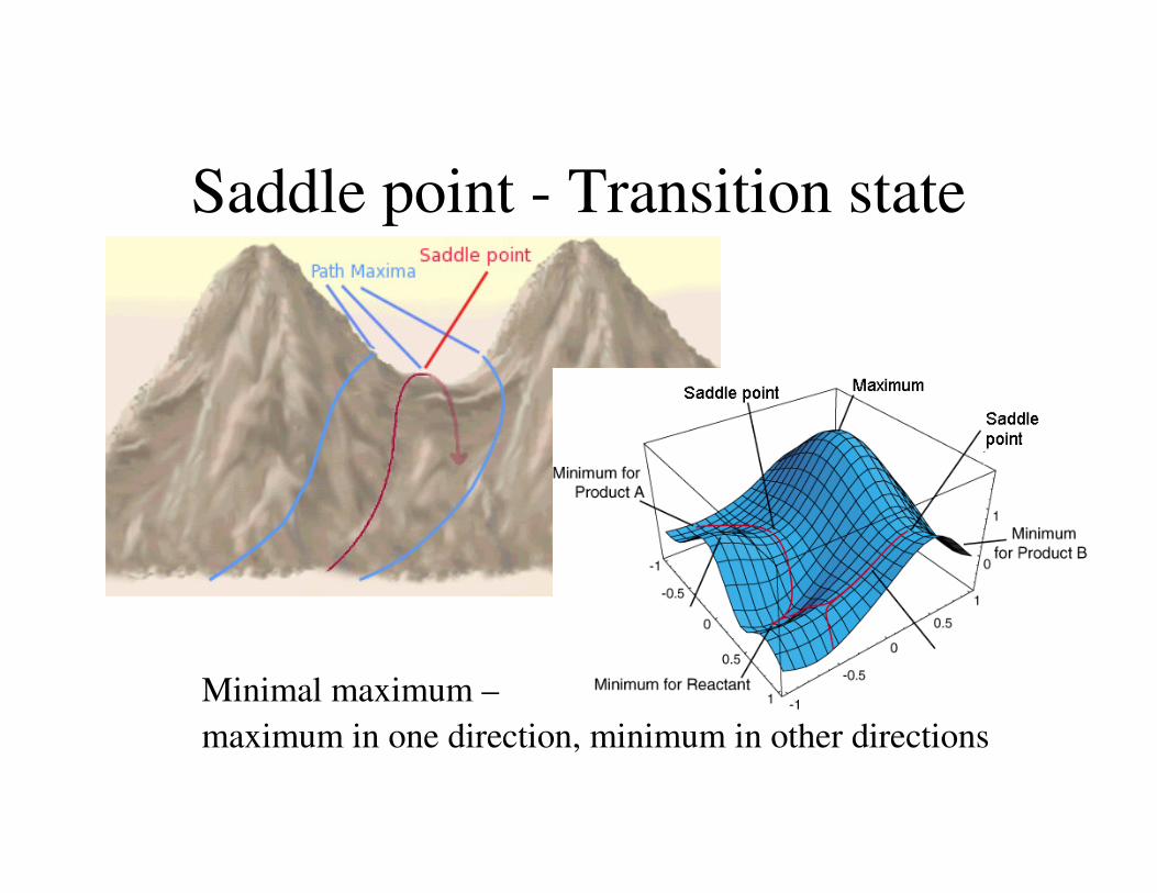
Saddle point - Transition state
Minimal maximum –
maximum in one direction, minimum in other directions
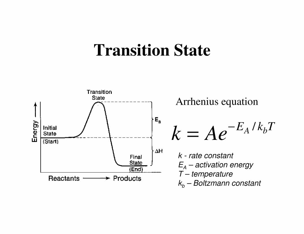
Transition State
/A bE k Tk Ae
−=
k - rate constant
EA – activation energy
T – temperature
kb – Boltzmann constant
Arrhenius equation

Multidimensional Optimization
- gradient
∇ f=0 - Stationary Point (minimum, maximum, or saddle point)
Force: F=-∇ E (Potential energy)
The coordinates can be
Cartesian (x,y,z..),
or internal, such as
bondlength and angle
displacements)
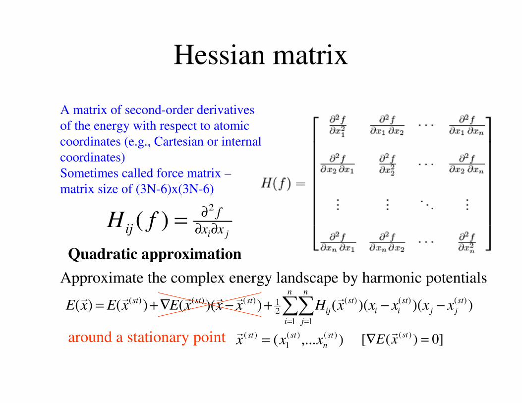
Hessian matrix
ji xx
f
ij fH∂∂
∂=
2
)(
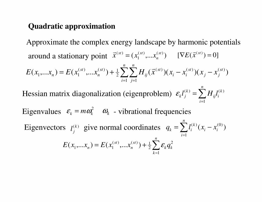
Quadratic approximation
around a stationary point
Approximate the complex energy landscape by harmonic potentials
A matrix of second-order derivatives
of the energy with respect to atomic
coordinates (e.g., Cartesian or internal
coordinates)
Sometimes called force matrix –
matrix size of (3N-6)x(3N-6)
),...( )()(
1
)( st
n
ststxxx =
r]0)([ )(
=∇st
xEr
∑∑= =
−−+−∇+=n
i
n
j
st
jj
st
ii
st
ij
ststst xxxxxHxxxExExE1 1
)()()(
21)()()( ))()(())(()()(
rrrrrr
∑=
=n
i
k
iij
k
jk lHl1
)()(εHessian matrix diagonalization (eigenproblem)
Eigenvalues2
kk mωε = kω - vibrational frequencies
Eigenvectors )(k
jl give normal coordinates ∑=
−=n
i
ii
k
ik xxlq1
)0()( )(
∑=
+=n
k
kk
st
n
st
n qxxExxE1
2
21)()(
11 ),...(),...( ε
∑∑= =
−−+=n
i
n
j
st
jj
st
ii
st
ij
st
n
st
n xxxxxHxxExxE1 1
)()()(
21)()(
11 ))()((),...(),...(r
Approximate the complex energy landscape by harmonic potentials
around a stationary point
Quadratic approximation
),...( )()(
1
)( st
n
ststxxx =
r]0)([ )(
=∇st
xEr

Eigenvalues2
kk mωε = kω - vibrational frequencies
Eigenvectors)(k
jl give normal coordinates ∑=
−=n
i
ii
k
ik xxlq1
)0()( )(
)real(0 All −> kk ωε
minimum
)imaginary(0 All −< kk ωε
maximum
)realimaginary/(0 −<> kk ωε
saddle point
Transition state – ε1<0, εk>0 (k>1)
Eigenvector l1- the path directionq
1
q2
∑=
+=n
k
kk
st
n
st
n qxxExxE1
2
21)()(
11 ),...(),...( ε

Algorithms for Finding Transition
StatesNo general methods which are guarantied to find!
Global methods – interpolation between reactant and product
Linear Synchronous Transit (LST)
Quadratic Synchronous Transit (QST)
Local methods – augmented Newton-Raphson
Eigenvector following
Berny algorithmSynchronous Transit-Guided Quasi-Newton (STQN)
method – QST+quasi-Newton
Force-field parameters in molecular mechanics are defined for equilibrium structures and can be inapplicable to transition structures.
Quantum calculations only
(recent semi-empirical potentials are applicable too)

Reactants
Saddle point
Products
Reactants
LST
Linear synchronous transit (LST)-search for a maximum along a linear path between reactants and products

Reactants
Saddle point
Products
Reactants
LST
QST
Linear synchronous transit (LST)- search for a maximum along a linear path between reactants and products
Quadratic synchronous transit (QST) - search for a maximum along an arc connecting reactants and products, and for a minimum in all directions perpendicular to the arc
Best case - the transition state is found.
General case – search is finished in a wrong saddle point or in a point with wrong number of negative eigenvalues (>1).
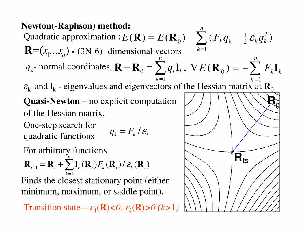
Newton(-Raphson) method:
One-step search for
quadratic functions kkk Fq ε/=
For arbitrary functions
Finds the closest stationary point (either
minimum, maximum, or saddle point).
Transition state – ε1(R)<0, εk(R)>0 (k>1)
Quasi-Newton – no explicit computation
of the Hessian matrix.
qk- normal coordinates, ,1
0 ∑=
=−n
k
kkq lRR ∑=
−=∇n
k
kkFE1
0 )( lR
Quadratic approximation : )()()( 2
21
1
0 kk
n
k
kk qqFEE ε∑=
−−= RR
εk and lk - eigenvalues and eigenvectors of the Hessian matrix at R0
)(/)()(1
1 ik
n
k
ikikii F RRRlRR ε∑=
+ +=
R 0
Rts
),...( 1 nxx=R - (3N-6) -dimensional vectors

Rational function optimization
(RFO)
∑=
+−
+=n
k kik
ikikii
F
1
1)(
)()(
λε R
RRlRR
ε1=min(εk) < λk≡λ<ε2/2
Berny algorithm (Gaussian, Opt=TS)
Eigenvector Following Method (Gaussian, Opt=EF; Hyperchem)
2/)4( 2
1
2
111 F++= εελ
∑>
−=≡>1
2 )/(:1i
iik Fk ελλλ
Clamber “up valley”
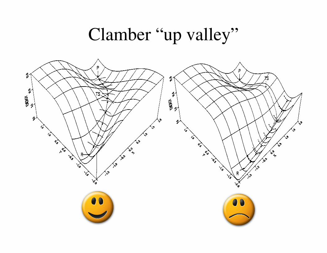
Clamber “up valley”

Synchronous Transit-Guided Quasi-Newton (STQN)
approach to the quadratic region -quadratic synchronous transit
complete the optimization-eigenvector-following algorithm
Reactants
Saddle point
Products
Eigenvector following
QST
TS estimateGaussian, Opt=QST2;
Hyperchem: input reactants and products only, automatic estimate of transition state
Gaussian, Opt=QST3: input reactants, products, and estimate of transition state

Is the correct TS found?
Look at the transition state geometry to make
sure it’s the right one.
Use several algorithms.
Try several estimates of transition state.
Follow reaction path to be sure that the
transition state connects the correct
reactants and products.

Reaction PathsSteepest descent path from transition state to reactants
and products
Gaussian - IRC
New point xk+1 –minimization on the hyperspheresurface
IRC-internal reaction coordinate


