
Timely and Non-Disruptive Response of Emergency Vehicles: AReal-Time Approach
Pratham Oza
Virginia Tech
Thidapat Chantem
Virginia Tech
ABSTRACTFacilitating timely traversal of emergency response vehicles (ERVs),
especially through an urban road network remains a challenging
task. ERV preemption is a technique commonly used to facilitate
prioritized ERV traversal. Unplanned deployment of ERV preemp-
tion can induce network-wide traffic delays. This paper presents
an ERV preemption strategy (considering ERV urgency levels) that
proactively manages the traffic before, during and after ERV traver-
sal by leveraging connected infrastructure to guarantee timely ERV
travel while minimizing traffic delays. We also provide worst-case
wait time bounds for non-emergency vehicles during ERV preemp-
tion. Our proposed approach does not introduce any additional
delay in ERV traversal over existing approaches while also showing
up to 43% reduction in average non-emergency traffic delays.
ACM Reference Format:Pratham Oza and Thidapat Chantem. 2021. Timely and Non-Disruptive
Response of Emergency Vehicles: A Real-Time Approach. In 29th Interna-tional Conference on Real-Time Networks and Systems (RTNS’2021), April7–9, 2021, NANTES, France. ACM, New York, NY, USA, 12 pages. https:
//doi.org/10.1145/3453417.3453434
1 INTRODUCTIONWith 70% of the world’s population expected to live in major urban
cities by 2050 [4], traffic congestion continues to be one of the most
pressing issues of urbanization. Most urban cities across the globe
have observed a 46–71% increase in traffic congestion [34]. Limited
space for urban expansion, especially for existing roadways creates
a bottleneck in meeting increasing traffic demands, due to which
efficient traffic management has become of prime importance.
Congested roadways not only lead to increased commute times,
fuel consumption and pollution, but also hamper timely deployment
of emergency response systems [3]. With over 240 million 911 calls
being made every year just in the US alone [1], emergency response
vehicles (ERVs) often fail to meet their target response time due
to congested roads and thereby affecting the hospitalization and
mortality rates [15]. Congestion further lead to queue spillbacks
This work was supported in part by the National Science Foundation under grant
numbers CPS-1658225 and CPS-2038726. We would like to thank the reviewers and
the shepherd for their suggestions that helped in improving the manuscript.
Permission to make digital or hard copies of all or part of this work for personal or
classroom use is granted without fee provided that copies are not made or distributed
for profit or commercial advantage and that copies bear this notice and the full citation
on the first page. Copyrights for components of this work owned by others than ACM
must be honored. Abstracting with credit is permitted. To copy otherwise, or republish,
to post on servers or to redistribute to lists, requires prior specific permission and/or a
fee. Request permissions from [email protected].
RTNS’2021, April 7–9, 2021, NANTES, France© 2021 Association for Computing Machinery.
ACM ISBN 978-1-4503-9001-9/21/04. . . $15.00
https://doi.org/10.1145/3453417.3453434
and collisions disrupting the entire road network. Queue spillbacks
occur when there is a queue downstream of an intersection that
disrupts the discharge of vehicles even when the light is green,
thereby propagating the congestion and causing a gridlock [27].
As a common practice, the non-emergency vehicle (non-ERV)
drivers are required to pull over to the edge of the roadway, when
an ERV is approaching, to allow its safe traversal [32] through
congested roads. However, in dense urban areas, the edges of the
roadways are often occupied by moving traffic or parked vehicles,
leading to confusion among the drivers when the ERV approaches.
In such situations, it is not only infeasible to clear the traffic for the
ERV but potentially dangerous, causing the non-ERVs and ERVs
to collide. The chances of an ERV getting into a crash are even
higher when it enters an intersection block with cross-traffic move-
ments [12]. Such situations make it difficult for the ERVs to quickly
and safely traverse through the road network and meet their re-
sponse times. Collisions further exacerbate the network-wide traffic
flow, making it difficult to restore smooth operations. Thus, the
traffic lights at an intersection must detect and facilitate safe ERV
traversal, known as ERV preemption, while reducing the traffic de-
lays for non-ERV movements caused by the preemption.
In most existing ERV preemption techniques, the intersections
independently control the traffic lights upon detecting an ERV [38].
However, failure to detect an ERV especially in heavy traffic, ham-
pers the ERV’s travel. The network-wide ERV preemption approaches
[5] switch multiple traffic lights to green when an ERV arrival is
expected while turning the lights for cross-traffic movements to red.
Such techniques facilitate ERV traversal, but fail to minimize its
impact on non-ERV traffic leading to propagated spillbacks, which
may in-turn worsen the traversal time of other imminent ERVs [6].
Existing work either provide ERV preemption mechanisms with-
out reducing its impact on the non-ERVs [21] or optimize traffic
flows through a network without facilitating ERVs [26]. However,
by leveraging the connected infrastructure, ERV arrival information
can be acquired well in time to not only facilitate smoother and safer
ERV traversal but also reduce the queues in the cross-traffic move-
ments such that the delays after ERV preemption are minimized.
By translating a typical traffic network with both, non-emergency
and emergency vehicles into a real-time task scheduling problem,
we present an end-to-end ERV preemption technique that enables
safe and quick ERV traversal. Using a deadline-driven approach,
we also optimally control the network-wide traffic before, duringand after the ERV traversal to minimize queues and reduce traffic
delays. We highlight the following contributions of this paper:
• We provide an ERV preemption strategy that provides a safe
and timely ERV passage through a road network of multiple
intersections while optimally managing non-emergency traffic.
1

RTNS’2021, April 7–9, 2021, NANTES, France Oza et al.
• By leveraging real-time ERV arrival and traffic data, our approach
optimally manages the network-wide traffic before the ERV ar-
rives and after the ERV safely traverses, such that guaranteed
timely ERV response is accompanied with reduced queues.
• By using the triage scale [9] (Table 2), we propose a priority-based
deadline-driven ERV preemption mechanism.
• We provide worst-case performance analysis for the non-ERV in
presence of an ERV to enhance the predictability of emergency
dispatch and traffic management systems.
• We analyze the adaptability of our approach using large-scale
simulations and hardware-in-loop (HIL) testbed with robots that
mimic human-driven vehicles through urban environment.
2 RELATEDWORKThe majority of the incidents involving ERVs occur due to collisions
within the intersection [6]. Traffic lights in the US are therefore
equipped with detectors, such as the 3M Opticom™ [28] using
infrared and GPS communication, or IoT-based approaches with
multiple sensors [18]. Such approaches are not only vulnerable to
interference, but also lead to longer queues at the intersections
downstream in urban areas due to the lack of coordination [19].
ERV traversal through a network of intersections is enabled
by green wave coordination [16] where consecutive traffic lights
along the ERV’s path are turned green after a constant offset-based
time delay or a fuzzy decision-making process [5]. However, such
heuristic mechanisms, lead to prolonged red lights for the conflict-
ing flows causing long wait-times and possible spillbacks [17]. We
discuss in our evaluation (Section 6) that our approach improves
the ERV travel time as compared to the existing work, while also
reducing the network-wide non-ERV traffic delays.
ERV preemptionwith connected and autonomous vehicles (CAVs)
present in the traffic is studied in [13, 36] that utilize vehicle-to-
everything (V2X) and cloud connectivity to gather real-time traffic
information and control each vehicle for ERV preemption. The pres-
ence of 100% CAVs on road however, is not expected until 2050 [10].
While we leverage basic connectivity between intersections within
our road network to disseminate ERV information, our approach is
applicable for conventional, mixed and autonomous traffic.
Conversely, the existing traffic approaches that optimize traffic
for a road network do not consider ERV preemption [20]. The exist-
ing work [25, 26] proposed a task model to represent traffic through
an intersection or a network of intersections. Specifically, in [26],
a recovery mechanism to counter unexpected traffic disruptions
using optimal strategies was provided. However, facilitating ERV
movements through the road network was not addressed. In this
paper, we leverage the real-time task model for a road network to
provide timeliness and safety guarantees for ERV traversal while
ensuring predictable traffic flow through the network.
The available ERV preemption mechanisms are heuristic and fail
to minimize the ERV’s impact on network-wide traffic and vice-
versa. The existing traffic control strategies minimize travel time
through the road network but they do not allow ERV preemption.
In our work, we propose an end-to-end solution that utilizes real-
time traffic and ERV arrival information to a) ensure timely ERV
traversal, b) proactively organize traffic before ERV arrival to reduce
traffic delays, and c) clear congestion after ERV traversal.
3 SYSTEM MODELA real-time task model to represent traffic flows through a road
network was proposed in [26]. In this paper we extend the task
model to accommodate for prioritized ERV traversals.
3.1 Road Network and Traffic LightsFor our model, we use a Manhattan grid-like𝑚 × 𝑛 road network
formed by𝑚 and𝑛 arterials travelling along the east-west and north-
south direction, respectively. Therefore, there are𝑚𝑛 intersections
in our road network. Such a network can either be standalone or
a part of a larger urban area. An intersection is formed by four
arterials, each traveling in a different direction, where the traffic
flow within each arterial is controlled by a traffic light. Each arterial
passes through multiple intersections across the network forming
links that connect two consecutive intersections. For example, in a
3 × 3 network, there are nine intersections formed by three arteri-
als traveling along the north-south and east-west directions each
(Figure 1). The traffic moving along the north and the south (or
the east and the west) direction within each arterial can enter the
intersections at once without interfering with one another and are
therefore called non-conflicting pairs of directions. However, the
vehicles traveling along the east-west direction conflict the vehicleflow along the north-south direction, and vice-versa, and cannot
access the intersections simultaneously. We use the following nota-
tions to throughout the paper to identify the links, arterials, and
intersections within the network:
• D,Dc: directions of traffic flow, where 𝐷 ∈ {𝑁, 𝐸,𝑊 , 𝑆} (car-dinal directions) and complementary, non-conflicting pairs of
directions, where 𝐷𝑐 ∈ {𝑆𝑁, 𝐸𝑊 }, respectively.• m, n: number of arterials in east-west and north-south directions,
respectively.
• 𝜶, 𝜶𝒓 : dummy operators, where 𝛼 = 𝑖 𝑗, 𝑖 ∈ [1,𝑚], 𝑗 ∈ [1, 𝑛],
𝛼𝑟 =
{𝑖𝑟,where 𝑖 ∈ [1,𝑚], 1 ≤ 𝑟 ≤ 𝑛, if 𝐷 ∈ {𝑆, 𝑁 }𝑟𝑖,where 1 ≤ 𝑟 ≤ 𝑚, 𝑖 ∈ [1, 𝑛], if 𝐷 ∈ {𝐸,𝑊 }.
• 𝑨𝑫𝜶𝒓
: 𝑟𝑡ℎ arterial for traffic in direction 𝐷 (Figure 1).
• 𝑳𝑫∗𝜶 : a link within an arterial such that multiple links connect
consecutive intersections to form an arterial. Here, ∗ denotes oneor more lanes within each link and is dropped when the context
is clear (Figure 1).
• 𝑰𝜶 : an intersection within the𝑚 × 𝑛 network (Figure 1).
• 𝑰𝒓𝒓 ′ : intersection formed by arterials 𝐴𝐷𝛼𝑟
and 𝐴𝐷′𝛼𝑟 ′ (Figure 1).
Traffic lights at each intersection within the network allow only
the non-conflicting flows to enter and access the intersection at
once, as per the phase sequences.Similar to [25, 26], our model considers that the traffic flow
within the𝑚 × 𝑛 network is managed by a traffic manager (TM),
denoted by 𝑇𝑀𝑚,𝑛 , that aggregates real-time traffic information
within the network from traffic sensors, forecast data and/or from
neighboring TMs. The TMs then control the traffic lights as per
some traffic control technique. We assume that the relevant data is
made available to the TM through minimal connectivity between
the intersections. Explicitly defining how such data is acquired
is out of scope of this work. The connected infrastructure is also
2

Timely and Non-Disruptive Response of Emergency Vehicles: A Real-Time Approach RTNS’2021, April 7–9, 2021, NANTES, France
Table 1: Glossary of notationsNotation Description
𝑻𝒄 Traffic cycle length (Sec. 3.2).
𝒂𝑫𝜶 , 𝒒𝑫𝜶 , 𝒛𝑫𝜶 Arrival rate, vehicle queue and the capacity of link 𝐿𝐷𝛼 (Sec. 3.2).
𝒍𝑫𝜶 , 𝒗𝒍 , 𝒅𝒔𝒂𝒇 𝒆Length of the link 𝐿𝐷𝛼 , vehicle length and
safe distance between consecutive vehicles (Sec. 3.2).
𝒉, 𝒕𝒍 Saturation headway and lost time [11].
𝒏𝑫𝜶,𝒌
, 𝑻𝒌Number of vehicles discharged in the 𝑘𝑡ℎ traffic cycle
from the link 𝐿𝐷𝛼 , and the time taken for the same(Equation 1).
𝒗𝒆 , 𝒍𝒆 , 𝒔𝒆 , 𝝅𝒆 , 𝜹Emergency response vehicle (ERV), location coordinates, the desired
speed, the priority level and delay tolerance of the ERV (Sec. 3.3).
𝑺𝑺 , 𝑩𝑺 , 𝑻𝑺 Sporadic server, its assigned budget and its inter-arrival time (Sec. 5.1).
𝑰 𝒆 , 𝑳𝒆The list of coordinates of the intersections and links
along the ERV route (Sec. 5.2).
𝑳𝑫1 , 𝑳𝑫𝝀
The first and the _𝑡ℎ link coordinates on the ERV’s route (Sec. 5.2).
𝝉𝒆 , 𝒂𝒆 , 𝒅𝒆ERV task, the arrival time and the deadline for the ERV task (Sec. 5.2).
𝒋𝒆𝒊 , 𝒂𝒆𝒊 , 𝑪
𝒆𝒊 , 𝒅
𝒆𝒊
𝑖𝑡ℎ sub-job of the ERV task, the arrival time,
the execution time and the deadline of the 𝑖𝑡ℎ sub-job (Sec. 5.2).
𝑼𝑫𝜶 % utilization for the server at link 𝐿𝐷𝛼 .
𝑼𝑫𝒄𝜶
% utilization such that𝑈𝐷𝑐𝛼 = 𝑈𝑆
𝛼 = 𝑈𝑁𝛼 , if 𝐷𝑐 = 𝑆𝑁 ,
and𝑈𝐷𝑐𝛼 = 𝑈𝑆
𝛼 = 𝑈𝑊𝛼 , otherwise (Sec. 5.3).
𝑼𝑫𝒄𝒎𝒊𝒏𝜶
, 𝑼𝑫𝒄𝒎𝒂𝒙𝜶 Minimum and maximum utilization demands (Sec. 5.3).
𝒕𝒔𝒕𝒂𝒓𝒕 , 𝒕𝒏𝒘Time of receiving the ERV arrival information
and duration between 𝑡𝑠𝑡𝑎𝑟𝑡 and 𝑑𝑒 (the ERV deadline) (Algorithm 2).
𝒏𝒏𝒘 , 𝒕𝒄𝒍𝒆𝒂𝒓Total vehicles expected within 𝑡𝑛𝑤and time to clear the vehicles respectively (Algorithm 2).
𝒒𝒆𝒊 Vehicle queue in the links during compensation phase (Algorithm 3).
𝑼𝑫𝒄𝜶𝒆 , 𝑼
𝑫′𝒄
𝜶𝒆% utilization for the complementary server pairs along the ERV route
and the server pairs along the links conflicting the ERV route (Sec. 5.3).
used to acquire ERV information which will be discussed in de-
tail (Section 5.2). Additionally, the size of the 𝑚 × 𝑛 network is
determined as per the feasibility of reliable connectivity among
the traffic infrastructure, communication latency overhead, avail-
able computational resources to perform calculations in real-time
and the traffic signal coordination requirements as per the U.S.
Department of Transportation guidelines [22].
3.2 Non-Emergency Traffic FlowThe traffic lights at each intersection within the network change
between green-yellow-red states as per the assigned timings. Each
traffic light changes its state once in a cyclic pattern based on the
phase sequence and cycle time (𝑇𝑐 ). With some connectivity among
the traffic infrastructure, multiple intersections can be coordinated,
especially in tightly-spaced urban traffic environment, such that all
intersections within the purview of a TM have a fixed𝑇𝑐 value [22].
The phases of the traffic lights at consecutive intersections are then
activated based on the traffic control technique to avoid queue spill-
backs and reduce traffic wait-times [26]. An incoming link 𝐿𝐷𝛼 is
𝑳𝟏𝟏𝑬 𝑳𝟏𝟐
𝑬 𝑳𝟏𝟑𝑬
𝑳𝟐𝟏𝑬 𝑳𝟐𝟐
𝑬 𝑳𝟐𝟑𝑬
𝑳𝟑𝟏𝑬 𝑳𝟑𝟐
𝑬 𝑳𝟑𝟑𝑬
𝑳𝟏𝟏𝑾 𝑳𝟏𝟐
𝑾 𝑳𝟏𝟑𝑾
𝑳𝟐𝟏𝑾 𝑳𝟐𝟐
𝑾 𝑳𝟐𝟑𝑾
𝑳𝟑𝟏𝑾 𝑳𝟑𝟐
𝑾 𝑳𝟑𝟑𝑾
𝑳𝟑𝟏
𝑺𝑳𝟐𝟏
𝑺𝑳𝟏𝟏
𝑺
𝑳𝟑𝟐
𝑺𝑳𝟐𝟐
𝑺𝑳𝟏𝟐
𝑺
𝑳𝟑𝟑
𝑺𝑳𝟐𝟑
𝑺𝑳𝟏𝟑
𝑺
𝑳𝟏𝟑
𝑵𝑳𝟐𝟑
𝑵𝑳𝟑𝟑
𝑵
𝑳𝟏𝟐
𝑵𝑳𝟐𝟐
𝑵𝑳𝟑𝟐
𝑵
𝑳𝟏𝟏
𝑵𝑳𝟐𝟏
𝑵𝑳𝟑𝟏
𝑵
𝑰𝟏𝟏 𝑰𝟏𝟐 𝑰𝟏𝟑
𝑰𝟐𝟏 𝑰𝟐𝟐 𝑰𝟐𝟑
𝑰𝟑𝟏 𝑰𝟑𝟐 𝑰𝟑𝟑
𝑨𝜶𝟏𝑬
𝑨𝜶𝟐𝑬
𝑨𝜶𝟑𝑬
𝑨𝜶𝟏𝑾
𝑨𝜶𝟐𝑾
𝑨𝜶𝟑𝑾
𝑨𝜶𝟏
𝑺
𝑨𝜶𝟐
𝑺
𝑨𝜶𝟑
𝑺
𝑨𝜶𝟏
𝑵
𝑨𝜶𝟐
𝑵
𝑨𝜶𝟑
𝑵
Figure 1: A typical 3 × 3 road network [26]
ERV dispatch
Calculate ERV arrival time
and deadlines (Alg. 1)
TM activates
Optimize network-wide traffic lights as
per mechanism (Sec. 5.4)
Select ERV preemption mechanism
(Alg. 2)
Find additional delay tolerance
using triage scale (Tab.1)
ERV passed?Trigger recovery
phase (Sec. 5.4.3)Proactive Preemption Critical Preemption
•100% budget for servers with ERV task•0% budget for conflicting servers
Mechanism as per Algorithm 2
•Reserved budget for servers with ERV task as per priority•Allow conflicting flows to avoid long queues during ERV traversal
Figure 2: TM task flow and preemption mechanisms
characterized by the tuple {𝑎𝐷𝛼,𝑘
, 𝑞𝐷𝛼,𝑘
, 𝑧𝐷𝛼 }, where 𝑎𝐷𝛼,𝑘 is the incom-
ing non-emergency vehicle flow rate, 𝑞𝐷𝛼,𝑘
is the number of vehicles
queued in the link during the 𝑘𝑡ℎ traffic cycle, and 𝑧𝐷𝛼 is the linkcapacity, i.e., the maximum number of vehicles that can enter a
link before spillback occurs, and the remaining notations are as
explained earlier. As per [25], the link capacity can be estimated
as 𝑧𝐷𝛼 =𝑙𝐷𝛼
𝑣𝑙+𝑑𝑠𝑎𝑓 𝑒 , where 𝑙𝐷𝛼 is the length of the link 𝐿𝐷𝛼 and 𝑣𝑙 and
𝑑𝑠𝑎𝑓 𝑒 denote the average vehicle length and safe distance required
between any two consecutive vehicles, respectively. The incoming
non-emergency vehicle flow rate, 𝑎𝐷𝛼,𝑘(𝑡) is a time-varying quantity,
however, in a given traffic cycle, under dynamic traffic conditions,
the worst-case traffic flow can be bounded based on traffic infor-
mation from the intersections. We thus refer to 𝑎𝐷𝛼,𝑘(𝑡) as 𝑎𝐷
𝛼,𝑘for
the rest of the paper to determine non-ERV flow rates. When the
traffic lights change and vehicles are allowed to cross the intersec-
tion, the discharge pattern is represented by the saturation headwaymodel [31] and is given by,
𝑇𝑘 = ℎ · 𝑛𝐷𝛼,𝑘+ 𝑡𝑙 . (1)
Here, 𝑇𝑘 denotes the time required to discharge 𝑛𝐷𝛼,𝑘
vehicles from
link 𝐿𝐷𝛼 during the 𝑘𝑡ℎ traffic cycle when the saturation headway
ℎ = 2 s and the lost time 𝑡𝑙 = 4 s are considered, respectively [11].
3.3 Emergency Response VehiclesThe emergency vehicles are often guided by a back-end dispatch
system with various routing mechanisms to calculate the optimum
path from its origin to the emergency location [29]. By leveraging
V2X connectivity between the ERV (or the back-end system) and
the connected infrastructure, the intersections within our𝑚 × 𝑛road network that will be affected by the ERV traversal can be
identified in advance. The ERVs’ arrival information can then be
disseminated to the TM to allow safe and timely traversal of the ERV.
In our model, an incoming ERV is denoted by 𝑣𝑒 and is represented
by the tuple, {𝑙𝑒 , 𝑠𝑒 , 𝜋𝑒 }. Here, 𝑙𝑒 , 𝑠𝑒 , and 𝜋𝑒 denote the current lo-cation coordinates, the desired speed and the priority level of an
ERV. We schedule the traffic such that the ERV maintains its fixed
desired speed. The arrival times and the deadlines are assigned to
the ERV based on the priority level defined by the triage scale [9].
Preempting multiple ERVs at once is left for future work.
Setting priorities as per the triage levels. Triage scale [9] providescritical ERV information that is already being utilized in emergency
and disaster management to establish prioritized time frames for
3
RTNS’2021, April 7–9, 2021, NANTES, France Oza et al.
𝝉𝟏(2,4)
𝝉𝟐(4,7)𝝉𝟑(5,8)
Aperiodic Tasks 𝝉𝒊(𝒓𝒊, 𝒄𝒊)
Sporadic Server
𝑺𝑺(𝑩𝑺, 𝑻𝑺)
Aperiodic Task Queue
Traffic Manager Task 𝑻𝑴𝒎,𝒏(𝑪𝑻𝑴, 𝒂𝑻𝑴)
Intersection(Shared Resource)
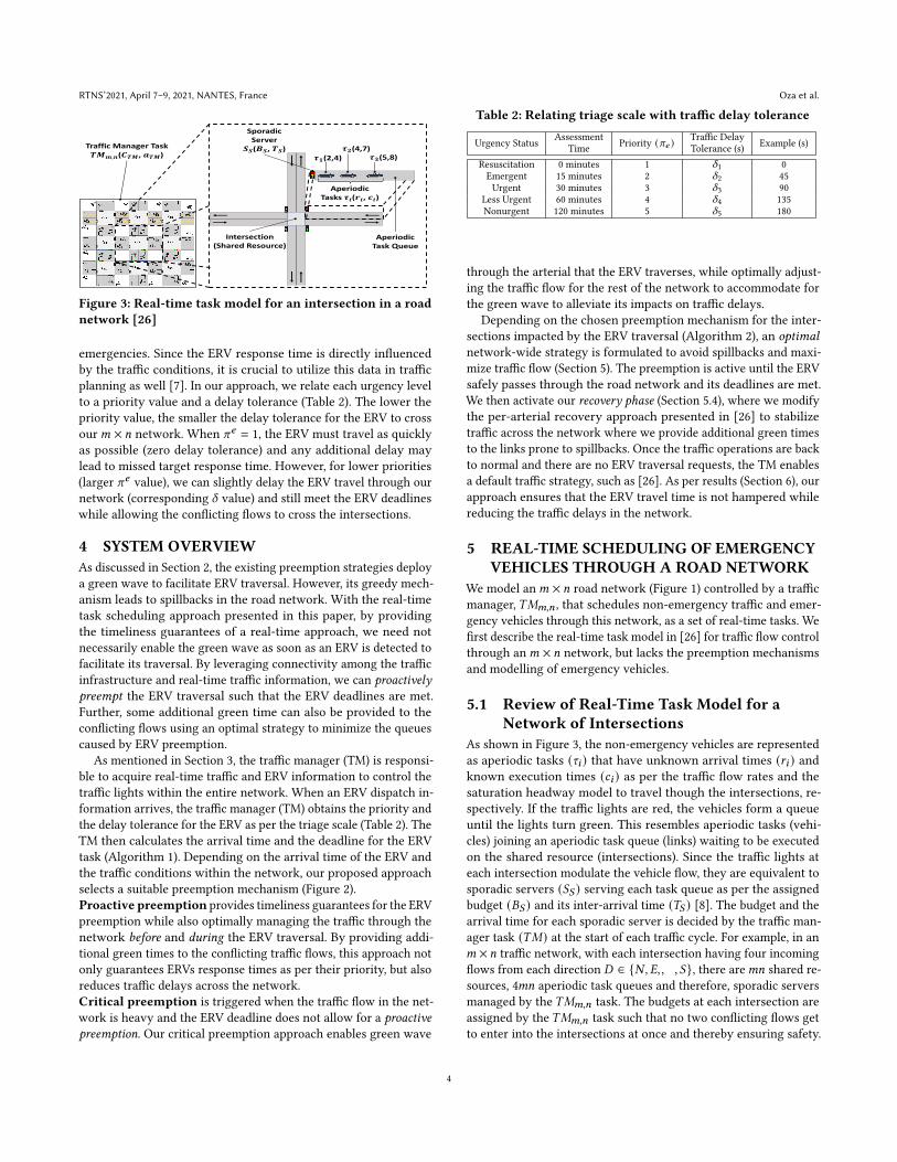
Figure 3: Real-time task model for an intersection in a roadnetwork [26]
emergencies. Since the ERV response time is directly influenced
by the traffic conditions, it is crucial to utilize this data in traffic
planning as well [7]. In our approach, we relate each urgency level
to a priority value and a delay tolerance (Table 2). The lower the
priority value, the smaller the delay tolerance for the ERV to cross
our𝑚 × 𝑛 network. When 𝜋𝑒 = 1, the ERV must travel as quickly
as possible (zero delay tolerance) and any additional delay may
lead to missed target response time. However, for lower priorities
(larger 𝜋𝑒 value), we can slightly delay the ERV travel through our
network (corresponding 𝛿 value) and still meet the ERV deadlines
while allowing the conflicting flows to cross the intersections.
4 SYSTEM OVERVIEWAs discussed in Section 2, the existing preemption strategies deploy
a green wave to facilitate ERV traversal. However, its greedy mech-
anism leads to spillbacks in the road network. With the real-time
task scheduling approach presented in this paper, by providing
the timeliness guarantees of a real-time approach, we need not
necessarily enable the green wave as soon as an ERV is detected to
facilitate its traversal. By leveraging connectivity among the traffic
infrastructure and real-time traffic information, we can proactivelypreempt the ERV traversal such that the ERV deadlines are met.
Further, some additional green time can also be provided to the
conflicting flows using an optimal strategy to minimize the queues
caused by ERV preemption.
As mentioned in Section 3, the traffic manager (TM) is responsi-
ble to acquire real-time traffic and ERV information to control the
traffic lights within the entire network. When an ERV dispatch in-
formation arrives, the traffic manager (TM) obtains the priority and
the delay tolerance for the ERV as per the triage scale (Table 2). The
TM then calculates the arrival time and the deadline for the ERV
task (Algorithm 1). Depending on the arrival time of the ERV and
the traffic conditions within the network, our proposed approach
selects a suitable preemption mechanism (Figure 2).
Proactive preemption provides timeliness guarantees for the ERV
preemption while also optimally managing the traffic through the
network before and during the ERV traversal. By providing addi-
tional green times to the conflicting traffic flows, this approach not
only guarantees ERVs response times as per their priority, but also
reduces traffic delays across the network.
Critical preemption is triggered when the traffic flow in the net-
work is heavy and the ERV deadline does not allow for a proactivepreemption. Our critical preemption approach enables green wave
Table 2: Relating triage scale with traffic delay tolerance
Urgency Status
Assessment
TimePriority (𝜋𝑒 )
Traffic Delay
Tolerance (s)Example (s)
Resuscitation 0 minutes 1 𝛿1 0
Emergent 15 minutes 2 𝛿2 45
Urgent 30 minutes 3 𝛿3 90
Less Urgent 60 minutes 4 𝛿4 135
Nonurgent 120 minutes 5 𝛿5 180
through the arterial that the ERV traverses, while optimally adjust-
ing the traffic flow for the rest of the network to accommodate for
the green wave to alleviate its impacts on traffic delays.
Depending on the chosen preemption mechanism for the inter-
sections impacted by the ERV traversal (Algorithm 2), an optimalnetwork-wide strategy is formulated to avoid spillbacks and maxi-
mize traffic flow (Section 5). The preemption is active until the ERV
safely passes through the road network and its deadlines are met.
We then activate our recovery phase (Section 5.4), where we modify
the per-arterial recovery approach presented in [26] to stabilize
traffic across the network where we provide additional green times
to the links prone to spillbacks. Once the traffic operations are back
to normal and there are no ERV traversal requests, the TM enables
a default traffic strategy, such as [26]. As per results (Section 6), our
approach ensures that the ERV travel time is not hampered while
reducing the traffic delays in the network.
5 REAL-TIME SCHEDULING OF EMERGENCYVEHICLES THROUGH A ROAD NETWORK
We model an𝑚 × 𝑛 road network (Figure 1) controlled by a traffic
manager, 𝑇𝑀𝑚,𝑛 , that schedules non-emergency traffic and emer-
gency vehicles through this network, as a set of real-time tasks. We
first describe the real-time task model in [26] for traffic flow control
through an𝑚 × 𝑛 network, but lacks the preemption mechanisms
and modelling of emergency vehicles.
5.1 Review of Real-Time Task Model for aNetwork of Intersections
As shown in Figure 3, the non-emergency vehicles are represented
as aperiodic tasks (𝜏𝑖 ) that have unknown arrival times (𝑟𝑖 ) andknown execution times (𝑐𝑖 ) as per the traffic flow rates and the
saturation headway model to travel though the intersections, re-
spectively. If the traffic lights are red, the vehicles form a queue
until the lights turn green. This resembles aperiodic tasks (vehi-
cles) joining an aperiodic task queue (links) waiting to be executed
on the shared resource (intersections). Since the traffic lights at
each intersection modulate the vehicle flow, they are equivalent to
sporadic servers (𝑆𝑆 ) serving each task queue as per the assigned
budget (𝐵𝑆 ) and its inter-arrival time (𝑇𝑆 ) [8]. The budget and the
arrival time for each sporadic server is decided by the traffic man-
ager task (𝑇𝑀) at the start of each traffic cycle. For example, in an
𝑚 × 𝑛 traffic network, with each intersection having four incoming
flows from each direction 𝐷 ∈ {𝑁, 𝐸,𝑊 , 𝑆}, there are𝑚𝑛 shared re-
sources, 4𝑚𝑛 aperiodic task queues and therefore, sporadic servers
managed by the 𝑇𝑀𝑚,𝑛 task. The budgets at each intersection are
assigned by the 𝑇𝑀𝑚,𝑛 task such that no two conflicting flows get
to enter into the intersections at once and thereby ensuring safety.
4

Timely and Non-Disruptive Response of Emergency Vehicles: A Real-Time Approach RTNS’2021, April 7–9, 2021, NANTES, France
Algorithm 1: Calculating the ERV task parameters: arrival
time and deadline using Manhattan distance [33]
Input :𝐿𝐷1, 𝐿𝐷
_⊲ coordinates to the entry and exit points of the preemption
arterial
𝑙𝑒 , 𝑠𝑒 , 𝜋𝑒 ⊲ ERV parameters
Output :𝑎𝑒 , 𝑑𝑒 ⊲ arrival time and deadline for 𝜏𝑒
1 Function GetERVTaskParams(𝐿𝐷1, 𝐿𝐷
_, 𝑙𝑒 , 𝑠𝑒):
2 𝑑𝑖𝑠𝑡1 = ManhattanDistance(𝐿𝐷1, 𝑙𝑒 ) ⊲ distance to 𝐿𝐷
1
3 𝑑𝑖𝑠𝑡_ = ManhattanDistance(𝐿𝐷_, 𝑙𝑒 ) ⊲ distance to 𝐿𝐷
_
4 𝛿 = GetDelay(𝜋𝑒) ⊲ From Table 2
5 𝑎𝑒 =𝑑𝑖𝑠𝑡
1
𝑠𝑒⊲ arrival time as per desired speed
6 𝑑𝑒 =𝑑𝑖𝑠𝑡_𝑠𝑒+ 𝛿 ⊲ deadline as per triage scale
7 return 𝑎𝑒 , 𝑑𝑒
8 End Function
The servers arrive as per their arrival times are executed on the
shared resource until the assigned budget is exhausted.
5.2 Emergency Vehicles as Real-Time TasksThe following information is required by the TM in our approach. (i)
The route that the ERVwill access within our𝑚×𝑛 network, and (ii)
the information represented by the tuple {𝑙𝑒 , 𝑠𝑒 , 𝜋𝑒 } that containsthe location coordinates, the desired speed, and the priority level of
the ERV, respectively. Explicitly defining how such information is
made available to the TM is out of scope of this work, however, we
rely on existing communication between connected infrastructure,
connected ERVs and/or the back-end dispatch systems that plan for
the ERV’s route and response times. Since the arrival of the ERV is
at random, it resembles an aperiodic task.From the route information, the TM determines the location
coordinates of the intersections (𝐼𝑒 ) and links (𝐿𝑒 ) that the ERV will
traverse. For simplicity of representation, we assume that the ERV
traverses only in the east-west or the north-south direction through
our road network, similar to the non-emergency traffic. However,
our approach is applicable to the general case. For example, consider
an ERV 𝑣𝑒 , entering a 3×3 network (Figure 1) and traveling throughthe arterial 𝐴𝐷
𝛼2
. The intersections and links accessed by the ERV
are 𝐼𝑒 = {𝐼21, 𝐼22, 𝐼33} and 𝐿𝑒 = {𝐿𝐷1, 𝐿𝐷
2, 𝐿𝐷
3}, respectively. Thus
the TM task must assign the budget to the servers that serve the
links 𝐿𝐷1, 𝐿𝐷
2, and 𝐿𝐷
3to facilitate preemption.
The ERV task 𝜏𝑒 is represented by the tuple {𝑎𝑒 , 𝑑𝑒 } where 𝑎𝑒and 𝑑𝑒 denote the arrival time and the deadline of ERV task. The
arrival time indicates the time at which the ERV is expected to enter
our road network, and the deadline indicates the time before which
the ERV must exit our network to meet its priority-based response
time. The values of 𝑎𝑒 and 𝑑𝑒 are calculated by the TM task using
Algorithm 1. Since the𝑇𝑀 task is responsible to schedule non-ERV
traffic while also facilitate ERV traversals arriving at random, it
resembles an aperiodic task with unknown arrival time and fixed
execution times that assigns the server budgets (Figure 3).
The ERV task’s deadline is calculated as per the delay tolerance
for each urgency level (Algorithm 1). If the ERV has the highest
priority, it has no delay tolerance (𝛿1 = 0, as per Table 2). Therefore,
the deadline for a highest priority ERV task is equal to the travel
time of the ERV from its current location to the end of the network
at its desired speed (Line 6). The TM task schedules the non-ERV
Aperiodic Task𝝉𝒆(𝒂𝒆, 𝒅𝒆)
Sub-Job 𝒋𝟏𝒆(𝒂𝟏
𝒆 , 𝑪𝟏𝒆 , 𝒅𝟏
𝒆)Sub-Job
𝒋𝟐𝒆(𝒂𝟐
𝒆 , 𝑪𝟐𝒆 , 𝒅𝟐
𝒆)Sub-Job
𝒋𝟑𝒆(𝒂𝟑
𝒆 , 𝑪𝟑𝒆 , 𝒅𝟑
𝒆)
𝒂𝒆 = 𝒂𝟏𝒆
𝑪𝟏𝒆 𝑪𝟐
𝒆 𝑪𝟑𝒆
Time in 𝑳𝟐𝟏𝑬 + 𝑰𝟐𝟏 Time in 𝑳𝟐𝟐
𝑬 + 𝑰𝟐𝟐 Time in 𝑳𝟐𝟑𝑬 + 𝑰𝟐𝟑
𝒂𝟐𝒆 𝒂𝟑
𝒆 𝒅𝟑𝒆 = 𝒅𝒆
Time (s)
𝒂𝒆, 𝒅𝒆: arrival time and deadline of ERV task 𝝉𝒆
𝒂𝒊𝒆, 𝑪𝒊
𝒆, 𝒅𝒊𝒆 :
arrival time, execution time and deadline of sub-job 𝒋𝒊
𝒆
Figure 4: Modelling an ERV as an aperiodic real-time taskand its sub-jobs
traffic and the ERV through the network such that the ERV meets
the deadline since its failure leads to increased response times to
attend life-threatening emergencies.
To capture an ERV traversing through the arterial 𝐴𝐷𝛼𝑟
in a real-
time model, each ERV task 𝜏𝑒 consists of _ sub-jobs 𝑗𝑒𝑖,∀𝑖 ∈ [1, _]
where _ = 𝑛 if𝐷 ∈ {𝐸,𝑊 } and _ =𝑚 otherwise. Here, the execution
of the 𝑖𝑡ℎ sub-job 𝑗𝑒𝑖represents traversal of ERV in the link 𝐿𝐷
𝑖𝑟until it crosses the intersection 𝐼𝑖𝑟 . Each sub-job 𝑗𝑒
𝑖is represented
by the tuple, {𝑎𝑒𝑖,𝐶𝑒
𝑖, 𝑑𝑒
𝑖} denoting the arrival time, the execution
time and the deadline of the 𝑖𝑡ℎ sub-job, respectively. As shown in
Figure 4, the arrival time of the sub-job indicates approaching ERV,
the execution time indicates the time the ERV takes to traverse the
corresponding section of the route, and the deadline indicates the
time before which the sub-job must complete execution to avoid
missed ERV response times.
Property 1. An ERV task 𝜏𝑒 consisting of _ sub-jobs 𝑗𝑒1, 𝑗𝑒2, . . . , 𝑗𝑒
_,
has the following properties: (i) The arrival time 𝑎𝑒1of the sub-job 𝑗𝑒
1
is equal to the arrival time 𝑎𝑒 of the task 𝜏𝑒 . (ii) The deadline 𝑑𝑒_of
the sub-job 𝑗𝑒_is equal to the deadline 𝑑𝑒 of the task 𝜏𝑒 . And finally,
(iii) the arrival time 𝑎𝑒𝑖of the sub-job 𝑗𝑒
𝑖is equal to the completion
time of the previous sub-job 𝑗𝑒𝑖−1, 𝑖 = 2, . . . , _.
Property 1 ensures that the entire trajectory of the ERV is ac-
counted for by our real-time model. (i) and (ii) ensure that the
network-level arrival times and the deadlines of the ERV are trans-
lated to is sub-jobs. If the first sub-job 𝑗𝑒1arrives at any time after
the actual ERV arrival time, this means that the ERV is not being
promptly serviced, which could lead to delay, abrupt stop and go
movements, and unsafe driving conditions for the ERV. Alternately,
if the last sub-job 𝑗𝑒_has a deadline earlier than the task itself, the
ERV will have to travel faster than its desired speed to meet its
deadline leading to safety violations. Similarly, (iii) ensures the
continuity of the ERV’s trajectory. The 𝑖𝑡ℎ sub-job must arrive as
soon as the 𝑖-1𝑡ℎ (previous) sub-job completes execution (Figure 4)
to maintain the continuity of the ERV traversal without abruptly
stopping inside the intersection box.
Assigning local deadlines to the sub-jobs: From Figure 4, the
ERV task 𝜏𝑒 will meet its deadline only if each of its sub-job meet
their respective deadlines. Once the TM receives the ERV informa-
tion, we assign the deadlines to each sub-job to maintain the overall
deadline for the ERV task as per Lemma 1.
Lemma 1. Consider an ERV task 𝜏𝑒 with the arrival time anddeadline of 𝑎𝑒 and 𝑑𝑒 respectively, representing ERV traversal throughan 𝑚 × 𝑛 road network across the arterial 𝐴𝐷
𝛼𝑟, with _ sub-jobs 𝑗𝑒
𝑖
𝑖 = 1, . . . , _ corresponding to each segment consisting of the link 𝐿𝐷𝑖
5

RTNS’2021, April 7–9, 2021, NANTES, France Oza et al.
Servers for ERV
Servers for conflicting flow
𝒅𝒆𝒂𝟑𝒆𝒂𝟐
𝒆𝒂𝟏𝒆
𝒂𝟑𝒆𝒂𝟐
𝒆𝒂𝟏𝒆 𝒅𝒆
𝝅𝒆 = 𝟓
𝝅𝒆 = 𝟏
No conflicting server execution due to highest priority
Delayed deadline for lower priority with conflicting server execution
Delayed deadline due to lower priorityavoiding possible
spillbacks and congestion in
conflicting flows
Time (s)
Time (s)
Figure 5: An example server execution for ERV preemptionwith varying priorities
and intersection 𝐼𝑖𝑟 . If the traffic flow rate from each direction 𝐷 atthe intersection 𝐼𝑖𝑟 is given by 𝑎𝐷
𝑖𝑟, then the local deadline 𝑑𝑒
𝑖for the
𝑖𝑡ℎ sub-job is given by,
𝑑𝑒𝑖 ∝∑
𝐷∈{𝑁,𝐸,𝑊 ,𝑆 }𝑎𝐷𝑖 , (2)
such that,_∑𝑖=1
𝑑𝑒𝑖 = 𝑑𝑒 , (3)
where, _ =𝑚 if 𝐷 ∈ {𝑆, 𝑁 } and 𝑛 otherwise.
Proof: The higher the traffic flow in a link, the longer will be
the execution time of the corresponding sub-job (Figure 4). To
ensure that there is fair distribution of time to execute the sub-
jobs, the local deadlines must be proportional to the traffic flows
within the intersection (and hence the link). As per Equation 2,
a later deadline will be assigned to the sub-job if the net traffic
flow rate through an intersection is higher. Similarly, since the
arrival times of the sub-jobs are co-dependent as shown in the
Property 1, missing the deadline for one sub-job causes a cascading
effect and end-to-end deadline misses. If the summation of all the
local deadlines is less than the total end-to-end deadline, the ERV
may traverse quickly through the road network, but the conflicting
flows suffer from resource starvation. Alternately, if the summation
of the local deadlines is greater than the total end-to-end deadline
it would clearly lead to missed end-to-end deadlines due to the sub-
job precedence established in Property 1. Therefore, the deadline
distribution in Equation 2 must be constrained by Equation 3.
As shown in Figure 5, an ERV with a lower priority has a higher
delay tolerance, hence its deadline is later than that of the ERV
with the highest priority. Upon scheduling, while the ERV with the
highest priority must be executed as soon as it arrives, a lower pri-
ority ERV task execution can be delayed to schedule the conflicting
flows and still meet the deadline. With this task model for the ERV
and the non-ERV traffic, we now discuss the scheduling strategy to
provide timely traversal of the ERV through the road network.
5.3 Non-emergency Traffic Flow SchedulingWhen there is no ERV dispatched, the TM deploys a default traffic
control scheme. For our work, we use the network-wide traffic
control strategy provided in [26] as a default scheme. However, any
schedule-based traffic strategy maybe deployed at the TM. We now
briefly summarize the budget allocation strategy provided in [26]
and then provide the requirements to accommodate the ERVs.
Algorithm 2: Preemption mechanism based on ERV dead-
line and traffic flow
Input :𝑡𝑠𝑡𝑎𝑟𝑡 ⊲ ERV dispatch notification received
𝑎𝑒 , 𝑑𝑒 , 𝜋𝑒 ⊲ ERV arrival time, deadline and priority
{𝑎𝐷𝑖, 𝑞𝐷
𝑖, 𝑧𝐷
𝑖} ⊲ traffic of links in preemption arterial
Output :preemption ⊲ selected mechanism
1 Function SelectPreemption(𝑡𝑠𝑡𝑎𝑟𝑡 , 𝑎𝑒 , 𝑑𝑒 , 𝑎𝐷
𝑖, 𝑞𝐷
𝑖):
2 𝑡𝑛𝑤 = 𝑑𝑒 − 𝑡𝑠𝑡𝑎𝑟𝑡3 𝑛𝑎𝑟𝑟 = 𝑎𝐷
1𝑡𝑛𝑤 ⊲ vehicles expected to arrive within 𝑡𝑛𝑤
4 𝑞𝑠𝑢𝑚 =∑_
𝑖=1 𝑞𝐷𝑖
⊲ total vehicles in queue at 𝑡𝑠𝑡𝑎𝑟𝑡5 𝑛𝑛𝑤 = 𝑛𝑎𝑟𝑟 + 𝑞𝑠𝑢𝑚 ⊲ total vehicles expected within 𝑡𝑛𝑤6 𝑡𝑐𝑙𝑒𝑎𝑟 = 𝑛𝑛𝑤ℎ + 𝑡𝑙 ⊲ time to clear 𝑛𝑛𝑤 vehicles (Eq. 1)
7 if 𝑎𝑒 − 𝑡𝑠𝑡𝑎𝑟𝑡 > 𝑡𝑐𝑙𝑒𝑎𝑟 then8 return proactive preemption
9 else10 return critical preemption
11 End Function
In [26], the TM gathers the real-time traffic information from
each intersection within the 𝑚 × 𝑛 network and allocates some
budget and the arrival times for the sporadic servers in the network
such that no two conflicting flows enter the intersections at the
same time. For a non-emergency traffic flow only, there is no priority
involved and therefore all sporadic servers arrive at the same time,
at the start of each traffic cycle and are executed on the shared
resource in a round-robin fashion. As mentioned, when there is no
ERV arrival, for our approach, the TM controls the non-emergency
traffic using the strategy defined in [26] which ensures that all
traffic lights within the𝑚 ×𝑛 network are optimally managed such
that spillbacks do not occur at any place within the network, when
possible. To do so, the budget allocation across all the servers in
the network for each traffic cycle is formulated as an optimization
problem with the following objective and constraints:
maximize
∑𝑖=1...𝑚,𝑗=1...𝑛,
𝐷𝑐 ∈{𝑆𝑁,𝐸𝑊 }
𝑈𝐷𝑐𝛼 (4)
subject to𝑈𝐷𝑐
𝑚𝑖𝑛𝛼≤ 𝑈
𝐷𝑐𝛼 ≤ 𝑈
𝐷𝑐𝑚𝑎𝑥𝛼 , (5)
𝑈𝐷𝑐
𝛼−1 −𝑈𝐷𝑐𝛼 ≤ 𝑧
𝐷𝑐𝛼 ℎ
𝑇𝑐, (6)∑
𝐷𝑐 ∈{𝑆𝑁,𝐸𝑊 }𝑈𝐷𝑐𝛼 ≤ 1, (7)
where,𝑈𝐷𝑐
𝑚𝑖𝑛𝛼=ℎ · (𝑎𝑘 ·𝑇𝑐 + 𝑞𝑘 − 𝑧) + 𝑡𝑙
𝑇𝑐, (8)
𝑈𝐷𝑐𝑚𝑎𝑥𝛼 =
ℎ · (𝑎𝑘 ·𝑇𝑐 + 𝑞𝑘 ) + 𝑡𝑙𝑇𝑐
. (9)
Here, 𝑈𝐷𝑐
𝑚𝑖𝑛𝛼and 𝑈
𝐷𝑐𝑚𝑎𝑥𝛼 correspond to the minimum and the
maximum utilization demands for the server pairs at the inter-
sections 𝐼𝛼 , respectively. The minimum utilization demand is the
budget required to avoid spillbacks within any given link, while the
maximum demand represents the budget to dispatch all vehicles
and clear a link. Similarly,𝑈𝐷𝑐𝛼 corresponds to the assigned budget
for the server pairs at intersection 𝐼𝛼 . Since two non-conflicting
flows can access the intersection at once, 𝑈 𝑆𝑁𝛼 = 𝑈 𝑆
𝛼 = 𝑈𝑁𝛼 and
𝑈 𝐸𝑊𝛼 = 𝑈 𝐸
𝛼 = 𝑈𝑊𝛼 . Since the budget allocation translates to the
6

Timely and Non-Disruptive Response of Emergency Vehicles: A Real-Time Approach RTNS’2021, April 7–9, 2021, NANTES, France
Algorithm 3: Queues for ERV compensation phase
Input :𝑡𝑠𝑡𝑎𝑟𝑡 ⊲ ERV dispatch notification received
{𝑎𝑒𝑖}, {𝑑𝑒
𝑖} ⊲ arrival time and deadline of all sub-jobs
{𝑎𝐷𝑖, 𝑞𝐷
𝑖, 𝑧𝐷
𝑖} ⊲ traffic of links in preemption arterial
𝑇𝑐 ⊲ traffic cycle time
Output : {𝑞𝑒𝑖} ⊲ set of queues for each link
1 Function GetQueues(𝑡𝑠𝑡𝑎𝑟𝑡 , {𝑎𝑒𝑖 }, {𝑑𝑒𝑖 }, 𝑎𝐷𝑖 , 𝑞𝐷𝑖, 𝑧𝐷
𝑖,𝑇𝑐):
2 𝑡𝑟 = (𝑑𝑒1− 𝑡𝑠𝑡𝑎𝑟𝑡 )%𝑇𝑐
3 𝑛𝑒𝑐 =
⌊𝑑𝑒1−𝑡𝑠𝑡𝑎𝑟𝑡𝑇𝑐
⌋4 if 𝑡𝑟 < 𝑡𝑙 then5 𝑡𝑟+ = 𝑇𝑐 , 𝑛
𝑒𝑐− = 1
6 ⊲ 𝑡𝑙 : human reaction lost time
7 𝑛𝑟 =𝑡𝑟 −𝑡𝑙ℎ
8 𝑛𝑟𝑖𝑛 = 𝑎𝐷1𝑡𝑟
9 𝑞𝑒1← min(𝑛𝑟 − 𝑛𝑟𝑖𝑛 , 𝑧
𝐷1)
10 for 𝑖 = 2 . . . _ do11 𝑐𝑒
𝑖−1 = 𝑑𝑒𝑖−1 − 𝑎𝑒𝑖−1
12 𝑞𝑒𝑖← min(
𝑐𝑒𝑖−1−𝑡𝑙ℎ
, 𝑧𝐷𝑖)
13 return {𝑞𝑒𝑖}
14 End Function
green time for the traffic lights, maximizing the total budget al-
location across the network using Equation 4 implies increased
traffic flow and thereby reduce wait times. Similarly, the constraint
in Equation 5 enforces that resource starvation does not occur by
assigning at least the minimum utilization requirement (𝑈𝐷𝑐
𝑚𝑖𝑛𝛼) for
each server, while avoiding over-utilization by keeping the assign-
ment up to the maximum requirement (𝑈𝐷𝑐𝑚𝑎𝑥𝛼 ). The constraint in
Equation 6 ensures that the budget allocation between consecutive
intersections is such that no spillbacks occur in the system, when
possible, thereby avoiding any additional delays and network-wide
gridlocks. Finally, the constraint in Equation 7 ensures that the
assigned budgets at any given intersection do not exceed 100%.
5.4 Enabling ERV Preemption: Scheduling theERV tasks and its Sub-Jobs
As mentioned in Section 4, our goal is to ensure that the ERV meets
its required response time as per the urgency level of the situa-
tion while leveraging the possible delay tolerance of the ERVs to
schedule non-emergency conflicting traffic flows as well (Figure 5).
This avoids spillbacks due to the prolonged red lights for the con-
flicting traffic flows, while adhering to the ERV’s timeliness. To
facilitate ERV preemption through the traffic network, we propose
an ERV-aware traffic control strategy where, when there is no ERV
expected to enter in the network, the default optimal traffic control
strategy as in [26] is implemented. However, an ERV preemption
request may arrive at any time and hence, we deploy a polling
mechanism that constantly checks for ERV dispatch notifications
via the connected infrastructure such as the back-end dispatch sys-
tem, RSUs or an equipped ERV itself. Once a preemption request is
received, as shown in Figure 2, the TM task is activated to enable
an ERV-aware traffic optimization approach which makes budget
allocation and scheduling decisions by selecting one of the two
preemption mechanisms (Algorithm 2), i.e., proactive preemption
or critical preemption. As discussed, selection of the preemption
mechanism depends on the traffic flow as well as the ERV deadlines.
Upon activation, at time 𝑡𝑠𝑡𝑎𝑟𝑡 , the TM calculates the ERV task’s
arrival time (𝑎𝑒 ) and the deadline (𝑑𝑒 ) using Algorithm 1. Let us
consider, that the ERV requests preemption through the arterial
𝐴𝐷𝛼𝑟
to access our network, which comprises of links 𝐿𝐷𝑖with the
parameters {𝑎𝐷𝑖, 𝑞𝐷
𝑖, 𝑧𝐷𝑖} and intersections 𝐼𝑖𝑟 , 𝑖 = 1, . . . , _. Based
on the traffic flow rate (𝑎𝐷𝑖) and existing queues (𝑞𝐷
𝑖) within each
link of the arterial 𝐴𝐷𝛼𝑟, at the time of receiving the ERV informa-
tion (𝑡𝑠𝑡𝑎𝑟𝑡 ), the TM decides which mechanism, i.e., proactive or
critical preemption to trigger. As shown in Algorithm 2, the TM
calculates the duration (𝑡𝑛𝑤 ) between 𝑡𝑠𝑡𝑎𝑟𝑡 and the ERV deadline,
𝑑𝑒 (Line 2). It then estimates the total number of vehicles, 𝑛𝑛𝑤 , and
the corresponding time, 𝑡𝑐𝑙𝑒𝑎𝑟 (as per Equation 1) to dispatch 𝑛𝑛𝑤vehicles and clear the arterial for the ERV traversal (Line 5 and 6).
Finally, if the time taken to clear the network is not less than the
arrival time of the ERV task, we do not have any additional budget
to proactively control the conflicting flows, and critical preemption
must be triggered immediately (Line 7) to meet the deadlines. Else,
the proactive preemption can be safely triggered (Line 9) to alleviate
resource starvation for the conflicting links, while ensuring that
the ERV deadlines are met. As per the selected mechanism, the TM
task now allocates the budget as well as the arrival times for the
corresponding servers that serve the links through which the ERV
passes while optimizing the traffic through the entire network.
By leveraging the connected infrastructure, the TM will be noti-
fied about an incoming ERV, multiple traffic cycles before it enters
the traffic network, i.e, 𝑎𝑒 − 𝑡𝑠𝑡𝑎𝑟𝑡 > 𝑡𝑐𝑙𝑒𝑎𝑟 to maximize the ben-
efits of the proposed proactive compensation. However, in case
𝑎𝑒 − 𝑡𝑠𝑡𝑎𝑟𝑡 ≤ 𝑡𝑐𝑙𝑒𝑎𝑟 , there is not enough bandwidth to proactively
distribute budget for the conflicting flows and critical preemption is
activated. But, by controlling the traffic as per the arrival time and
the deadline of the ERV task and its sub-jobs, and optimizing traffic
for the network instead of a greedy green wave, we ensure that the
ERV traversal is not hampered while reducing overall traffic delays.
5.4.1 Scheduling with critical preemption. Critical preemption indi-
cates that the servers must dedicate their entire resources towards
facilitating the ERV traversal through the network (Figure 2). Let
the arterial throughwhich the ERV requests for traversal be denoted
by 𝐴𝐷𝛼𝑒
with the corresponding servers along the arterial and their
budgets be denoted by 𝑆𝐷𝑐𝛼𝑒 and 𝑈
𝐷𝑐𝛼𝑒 , respectively. The servers that
are serving the conflicting flows to this arterial and the correspond-
ing budgets are hence denoted by 𝑆𝐷′𝑐𝛼𝑒 and 𝑈
𝐷′𝑐𝛼𝑒 , respectively. Once
critical preemption is triggered, the TM employs an ERV-aware
optimization approach to calculate the budget allocation for the
servers within the𝑚 × 𝑛 network, formulated as follows:
maximize
∑𝑖=1...𝑚,𝑗=1...𝑛,𝑖 𝑗∉𝛼𝑒 ,
𝐷𝑐 ∈{𝑆𝑁 ,𝐸𝑊 }
𝑈𝐷𝑐𝛼 (10)
subject to𝑈𝐷𝑐𝛼𝑒 = 1,𝑈
𝐷′𝑐𝛼𝑒 = 0 (11)
𝑈𝐷𝑐
𝑚𝑖𝑛𝛼≤ 𝑈
𝐷𝑐𝛼 ≤ 𝑈
𝐷𝑐𝑚𝑎𝑥𝛼 , 𝛼 ≠ 𝛼𝑒 (12)
𝑈𝐷𝑐
𝛼−1 −𝑈𝐷𝑐𝛼 ≤ 𝑧
𝐷𝑐𝛼 ℎ
𝑇𝑐, 𝛼 ≠ 𝛼𝑒 (13)
Equation (7) .
7

RTNS’2021, April 7–9, 2021, NANTES, France Oza et al.
Here, 𝐷𝑐 , 𝐷′𝑐 ∈ {𝑆𝑁, 𝐸𝑊 } such that, if 𝐷𝑐 = 𝑆𝑁, 𝐷 ′𝑐 = 𝐸𝑊 , else
𝐷𝑐 = 𝐸𝑊 ,𝐷 ′𝑐 = 𝑆𝑁 . Since the main goal of ERV preemption is not
maximizing traffic flow but to facilitate ERV traversal first, through
the intersections the ERV passes through, the objective function
(Equation 10) only maximizes the traffic flow through the network
for the servers that are not serving the ERV task (𝑖 𝑗 ∉ 𝛼𝑒 ). Since the
arterial 𝐴𝐷𝛼𝑒
is impacted by ERV preemption, all servers along this
arterial are directly assigned 100% of the budget to facilitate rapid
traversal of the ERV (Equation 11). Further, the TM does not assign
any budget to the servers for the conflicting traffic flows to ensure
the safety of the ERV. Constraints given by the Equations 12 and 13
ensure that the rest of the network stays live and the flow is still
maximized while avoiding under-/over-utilization of the resources
and spillbacks. This ensures that the effect of the ERV preemption
remains localized and does not spread through the network as much
as possible. Finally, the schedulability constraint (Equation 7) that
ensures traffic safety is enforced for all servers within the network.
5.4.2 Scheduling in proactive preemption. Proactive preemption is
activated, as per Algorithm 2 when the ERV does not necessarily
require immediate preemption and the TM utilizes this time to pro-
vide additional budget to the flows conflicting the ERV movement.
The budgets in this mechanism are assigned, such that the vehicle
queues in the ERV’s arterial and its links are maintained using Al-
gorithm 3. The vehicle queues are chosen based on the arrival time,
deadline and the delay tolerance of the ERV task. The arrival time
and the budget for the sporadic servers are set such that when the
servers are executed, the vehicle queues are dispatched just in time
to enable smooth and safe ERV traversal and thereby meeting the
local sub-job deadlines (hence the ERV deadline). Upon selecting
the proactive preemption, we calculate the number of traffic cycles,
𝑛𝑒𝑐 of𝑇𝑐 time in the time span of receiving the ERV information and
the deadline, 𝑑𝑒1of the first sub-job 𝑗𝑒
1(Line 3). Then, we find the
remaining time to 𝑗𝑒1’s deadline (Line 2). If the remaining time (𝑡𝑟 )
is less than the start-up lost time (𝑡𝑙 ) which represents the reaction
time to the green light for the first vehicle in the queue, then 𝑡𝑟 is
not enough to dispatch even one vehicle, and hence, a cycle time
(𝑇𝑐 ) worth of time is added to 𝑡𝑟 while subtracting one cycle from 𝑛𝑒𝑐(Line 5). This operation ensures that there is enough time for human
driven vehicles to react to green lights and incoming ERVs without
making hasty traffic decision and thereby reinforcing safety. We
then find the number of vehicles (𝑛𝑟 ) that we can dispatch within
𝑡𝑟 as well as the number of vehicles (𝑛𝑟𝑖𝑛 ) that enter the arterial
𝐴𝐷𝛼𝑒
at the worst-case (Line 6 and 7). This indicates that a queue
of 𝑞𝑒1= 𝑛𝑟𝑖𝑛 − 𝑛𝑟 in the first link can exist and still meet the first
sub-job’s deadline if we start ERV preemption at time 𝑛𝑒𝑐 . The queue
is also bounded by the link capacity to avoid spillbacks (Line 8).
Enabling green-wave coordination. : Since missing one of the sub-
job’s deadlines for the ERV task leads to a cascading effect for
all sub-jobs (Property 1), when the sub-job 𝑗𝑒𝑖is being executed,
the next link (corresponding to sub-job 𝑗𝑒𝑖+1) must be ready by
dispatching all vehicles within, before 𝑗𝑒𝑖reaches its deadline and
finishes execution. Since completion time for a sub-job 𝑗𝑒𝑖is equal
to the arrival time for the next sub-job 𝑗𝑒𝑖+1, the queues in each link
must be maintained (not exceeding the link capacity) such that the
links can be cleared (all vehicles dispatched) by the time the sub-job
ERV
Intersections
Figure 6: HIL framework with two intersections and an ERV
for the previous link completes execution (Line 10 and 11). This
ensures that by the time the previous sub-job reaches its deadline,
the next sub-job is ready for execution.
Budget assignment for proactive preemption. Consider that the ERVpreemption and traversal is requested in the arterial 𝐴𝐷
𝛼𝑒and using
Algorithm 3 we can determine the queues we need to maintain such
that all sub-jobs of the ERV task meet their deadline, the ERV task
hence meets its end-to-end deadline and green-wave coordination
is also enabled to ensure minimum stop-and-go traffic for higher
priority ERVs as well as the non-ERVs. Thus, the utilization bounds
for each server 𝑆𝐷𝛼𝑒 , 𝑖 = 1, . . . , _ within the arterial 𝐴𝐷𝛼𝑒
with queue
estimated as 𝑞𝑒𝑖can be formulated as,
𝑈𝐷𝑚𝑖𝑛𝛼𝑒
=ℎ · 𝑞𝑒
𝑖+ 𝑡𝑙
𝑇𝑐. (14)
The ERV-aware traffic control with proactive preemption is formu-
lated as follows.
maximize(Equation 4)
subject to𝑈𝐷𝑐𝛼𝑒 ≥ 𝑈
𝐷𝑐
𝑚𝑖𝑛𝛼𝑒(15)
𝑈𝐷′𝑐𝛼𝑒 ≤ 𝑈
𝐷′𝑐𝑚𝑎𝑥𝛼𝑒
(16)
Equations (7), (12), (13).𝐷𝑐 and 𝐷 ′𝑐 are conflicting pairs of traffic flows, as defined earlier.
Unlike critical preemption, in proactive preemption constraints in
Equations 15 and 16 enable dedicating some budget to the conflict-
ing flows as long as the minimum utilization demands of the servers
serving the ERV are satisfied, which ensures that the ERV deadlines
are met for each sub-job. Constraints in Equation 12 and 13 ensure
that the under-/over-utilization of resources for servers serving the
links not affected by the ERV is avoided and the schedulability of
the system (Equation 7) is maintained. Thus, by assigning sub-job
specific deadlines for the ERV task based on priority and delay
tolerance given by the triage scale, proactive preemption provides a
more planned approach towards the ERV traversal by avoiding long
queues and spillbacks before and during the ERV traversal. The
preemption mechanisms (critical and proactive) stay in effect until
the deadline of the corresponding sub-job has passed, i.e., until 𝑑𝑒𝑖.
In all, the critical preemption as well as the proactive preemption
provide strategies to enable ERV traversal such that their deadlines
are met and also control network-wide traffic to reduce queues
and traffic delays. Since ERV preemption still remains a priority
in both the preemption mechanisms discussed, there may be sce-
narios where long queues and potential spillbacks are unavoidable.
Specifically, we show in Section 6, that when there are heavy traffic
8
Timely and Non-Disruptive Response of Emergency Vehicles: A Real-Time Approach RTNS’2021, April 7–9, 2021, NANTES, France
Table 3: Flow types simulated as per the trafficflow rates andits description as per the FHWA [23]
.
Flow Type
Flow rate per lane
(Net flow in 3 × 3 network) Description
Low
1–4 veh/min
(540–2100 veh/hr)
Network running under capacity
with reduced travel delays
Medium
4–6 veh/min
(2100–3200 veh/hr)
Network nearing capacity
with longer queues
Heavy
up to 8 veh/min
(up to 4300 veh/hr)
Unstable traffic flow
with long wait times
flows in the network, enabling ERV traversal may lead to poten-
tial spillbacks. For such cases, we extend the per-arterial recoveryapproach presented in [26] to stabilize the entire network.
5.4.3 Scheduling in recovery phase. A recovery approach address-
ing a single arterial experiencing spillbacks was presented in [26].
Due to the lack of ERV preemption in their approach, their recovery
strategy fails to address cases when multiple arterials within the
network have long queues and potential spillbacks. Since multiple
conflicting flows experience prolonged red lights due to the preemp-
tion, especially when critical preemption is deployed, the recovery
approach must be extended for multiple links and arterials. We
therefore formulate a network-wide recovery approach as follows.
maximize (Equation 4)
subject to𝑈𝐷𝑐𝛼𝑒 = 𝑈
𝐷𝑐
𝑚𝑖𝑛𝛼𝑒(17)
𝑈𝐷′𝑐𝛼𝑒 = 1 −𝑈𝐷𝑐
𝑚𝑖𝑛𝛼𝑒(18)
Equations (7), (12), (13).In the recovery phase, we assign minimum budget requirement
to the servers that recently serviced the ERV (Equation 17) while
maximizing traffic flow for the conflicting servers (Equation 18).
Along with the constraint in Equation 13, the traffic through all
arterials conflicting the ERV flow will be maximized (Equation 4)
since assigned budget at𝑈𝐷𝑐𝛼 depends on𝑈
𝐷𝑐
𝛼−1. The recovery phaseis replaced with the default traffic strategy after one traffic cycle.
Table 1 refers to frequently used notations for the readers.
5.5 Worst-Case Performance Analysis forERV-Aware Traffic Control
We now provide a worst-case analysis to predict the impact of
the ERV traversal on the non-ERV flow which can help the traffic
routing systems to predict existing delays in the network. Worst-
case traffic delay accounts for the total time that a vehicle has to stop
while traversing through the network. Theorem 1 [26], presents a
worst-case traffic delay analysis without ERV traversal.
Theorem 1 ([24]). Assuming that the traffic flow rate for vehiclesentering the arterial 𝐴𝐷
𝛼𝑟, traveling through all links 𝐿𝑖 is 𝑎𝑖 , the
cumulative wait time𝑊𝐷𝛼𝑟,𝑝
for a vehicle at the 𝑝𝑡ℎ position in the
queue upon entering the arterial in the 𝑘𝑡ℎ cycle is bounded by
𝑊𝐷𝛼𝑟,𝑝 ∈
0,
⌊𝑝
𝑛𝑜𝑢𝑡1𝑘
⌋∑𝑘=1
©«_𝑇𝑐 − _𝑈𝑚𝑖𝑛1,𝑘
𝑇𝑐 +_∑𝑖=2
(_ − 𝑖 + 1)𝑧𝑖ℎª®¬
(19)
where _ = 𝑛, if 𝐷 = {𝑆, 𝑁 }, and _ = 𝑚, otherwise. 𝑛𝑜𝑢𝑡1𝑘 is theminimum number of vehicles dispatched from link 𝐿1 of arterial 𝐴𝐷
𝛼𝑟
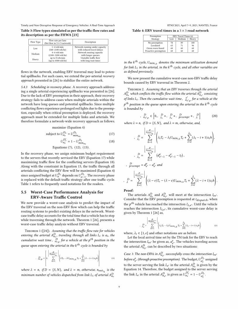
Table 4: ERV travel times in a 3 × 3 road networkPreemption
Strategy
ERV Travel Times (s)
Low Medium Heavy
No preemption 78 89 100
Localized 63 71 96
Green wave-based 60 60 60
Proactive preemption 60 60 60
in the 𝑘𝑡ℎ cycle, 𝑈𝑚𝑖𝑛1,𝑘denotes the minimum utilization demand
for link 𝐿1 in the arterial, in the 𝑘𝑡ℎ cycle, and all other variables areas defined previously.
We now present the cumulative worst-case non-ERV traffic delay
bounds caused by ERV traversal in Theorem 2.
Theorem 2. Assuming that an ERV traverses through the arterial𝐴𝐷𝛼𝑒
which conflicts the traffic flow within the arterial𝐴𝐷𝛼𝑒′ consisting
of links 𝐿𝑖 . Then the cumulative wait time𝑊 𝑒′𝛼𝑒′,𝑝 for a vehicle at the
𝑝𝑡ℎ position in the queue upon entering the arterial in the 𝑘𝑡ℎ cycleis bounded by
𝑊𝐷𝛼𝑒′,𝑝 ∈
[0,𝑊𝐷
_𝑖+𝑊𝐷
_𝑒+𝑊𝐷
𝑝𝑟𝑒𝑒𝑚𝑝𝑡 +𝑊𝐷_
](20)
where _ = 𝑛, if 𝐷 = {𝑆, 𝑁 }, and _ =𝑚, otherwise, and,
𝑊𝐷_𝑖
=
⌊𝑝
𝑛𝑜𝑢𝑡1𝑘
⌋∑𝑘=1
©«_𝑖𝑇𝑐 − _𝑖𝑈𝑚𝑖𝑛1,𝑘𝑇𝑐 +
_𝑖∑𝑖=2
(_𝑖 − 𝑖 + 1)𝑧𝑖ℎª®¬ ,
𝑊𝐷_𝑒
=
⌊𝑝
𝑛𝑜𝑢𝑡1𝑘
⌋∑𝑘=1
(𝑑𝑒𝑒′−1 − 𝑎
𝑒𝑒′−1 − 𝑡𝑙
),
𝑊𝐷𝑝𝑟𝑒𝑒𝑚𝑝𝑡 = 𝑑𝑒𝑒′ − 𝑎
𝑒𝑒′ and
𝑊𝐷_
=
⌊𝑝
𝑛𝑜𝑢𝑡1𝑘
⌋∑𝑘=1
((_ − 𝑒)𝑇𝑐 − (_ − 𝑒)𝑈𝑚𝑖𝑛1,𝑘
𝑇𝑐 +_∑𝑖=𝑒
(_ − 𝑖 + 1)𝑧𝑖ℎ).
Proof:The arterials 𝐴𝐷
𝛼𝑒and 𝐴𝐷
𝛼𝑒′ will meet at the intersection 𝐼𝑒𝑒′ .
Consider that the ERV preemption is requested at 𝑡𝑑𝑖𝑠𝑝𝑎𝑡𝑐ℎ , when
the 𝑝𝑡ℎ vehicle has reached the intersection 𝐼_𝑖𝑒′ . Until the vehicle
reaches the intersection 𝐼_𝑖𝑒′ , its cumulative worst-case delay is
given by Theorem 1 [26] as,
𝑊𝐷_𝑖
=
⌊𝑝
𝑛𝑜𝑢𝑡1𝑘
⌋∑𝑘=1
©«_𝑖𝑇𝑐 − _𝑖𝑈𝑚𝑖𝑛1,𝑘
𝑇𝑐 +_𝑖∑𝑖=2
(_𝑖 − 𝑖 + 1)𝑧𝑖ℎª®¬ , (21)
where, _𝑖 ∈ [1, 𝑒] and other notations are as before.
Let the local arrival time set by the TM task for the ERV to reach
the intersection 𝐼𝑒𝑒′ be given as, 𝑎𝑒𝑒′ . The vehicles traveling across
the arterial 𝐴𝐷𝛼𝑒′ can be described by two situations:
Case 1: The non-ERVs in 𝐴𝐷𝛼𝑒′ successfully cross the intersection 𝐼𝑒𝑒′
before𝑎𝑒𝑒′ (through proactive preemption). The budget,𝑈𝐷𝑐
𝛼′𝑒assigned
to the server serving the link 𝐿𝑒′ in the arterial 𝐴𝐷𝛼𝑒
is given by the
Equation 14. Therefore, the budget assigned to the server serving
the link 𝐿𝑒 in the arterial 𝐴𝐷𝛼𝑒′ is given as𝑈
𝐷′𝑐𝛼𝑒 = 1 −𝑈𝐷𝑐
𝛼′𝑒.
9
RTNS’2021, April 7–9, 2021, NANTES, France Oza et al.
Table 5: Effect of priority-based deadlines on overall trafficflow. 𝑐𝑒
𝑖and 𝑑𝑒
𝑖are the completion times and the deadlines
for the sub-job 𝑗𝑒𝑖of the ERV task arriving at 1100 s.
Priority
(𝜋𝑒 )𝑐𝑒1(s) 𝑑𝑒
1(s) 𝑐𝑒 (s) 𝑑𝑒
2(s) 𝑐𝑒
3(s)
𝑑𝑒3= 𝑑𝑒
(s)
Average Traffic
Delay (s)
1 1255 1255 1285 1285 1315 1315 39.97
2 1255 1274 1288 1296 1320 1330 36.75
3 1275 1285 1315 1315 1345 1345 35.45
4 1282 282 1315 1324 1350 1360 31.48
5 1307 1320 1345 1352 1383 1385 30.72
𝑳𝒊𝒋𝑬∗ (Link)
𝑰𝒊𝒊
𝑨𝜶𝒊𝑬 (Arterial)
𝑨𝜶𝒊𝑾
𝑨𝜶𝒊𝑺
𝑨𝜶𝒊𝑵
𝑳𝒊𝒋𝑺∗
𝑳𝒊𝒋𝑵∗
𝑳𝒊𝒋𝑾∗
(Servers)
Total Budget = 𝑻𝒄
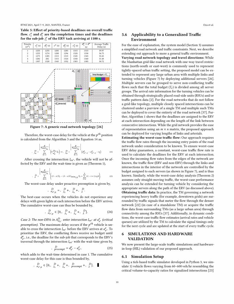
Figure 7: A generic road network topology [26]
Therefore, the worst-case delay for the vehicle at the 𝑝𝑡ℎ position
is calculated from the Algorithm 3 and the Equation 14 as,
𝑊𝐷_𝑒
=
⌊𝑝
𝑛𝑜𝑢𝑡1𝑘
⌋∑𝑘=1
(𝑈𝐷𝑐𝛼′𝑒
𝑇𝑐
)⇒𝑊𝐷
_𝑒=
⌊𝑝
𝑛𝑜𝑢𝑡1𝑘
⌋∑𝑘=1
(𝑑𝑒𝑒′−1 − 𝑎
𝑒𝑒′−1 − 𝑡𝑙
)(22)
After crossing the intersection 𝐼𝑒𝑒′ , the vehicle will not be af-
fected by the ERV and the wait-time is given as (Theorem 1),
𝑊𝐷_
=
⌊𝑝
𝑛𝑜𝑢𝑡1𝑘
⌋∑𝑘=1
©«(_ − 𝑒 )𝑇𝑐 − (_ − 𝑒 )𝑈𝑚𝑖𝑛1,𝑘
𝑇𝑐 +_∑𝑖=𝑒
(_ − 𝑖 + 1)𝑧𝑖ℎª®¬ , (23)
The worst-case delay under proactive preemption is given by,
𝑊𝐷𝛼𝑒′,𝑝 =𝑊𝐷
_𝑖+𝑊𝐷
_𝑒+𝑊𝐷
_.
The best-case occurs when the vehicles do not experience any
delays with green lights at each intersection before the ERV arrives.
The cumulative worst-case can thus be bounded by,
𝑊𝐷𝛼𝑒′,𝑝 ∈ [0,𝑊
𝐷_𝑖+𝑊𝐷
_𝑒+𝑊𝐷
_] . (24)
Case 2: The non-ERVs in 𝐴𝐷𝛼𝑒′ enter intersection 𝐼𝑒𝑒′ at 𝑎𝑒𝑒′ (critical
preemption). The maximum delay occurs if the 𝑝𝑡ℎ vehicle is un-
able to cross the intersection 𝐼𝑒𝑒′ before the ERV arrives at 𝑎𝑒𝑒′ . To
prioritize the ERV, the conflicting flows receive no budget until
𝑑𝑒𝑒′ , i.e., the deadline for the sub-job that corresponds to the ERV’s
traversal through the intersection 𝐼𝑒𝑒′ with the wait-time given by,
𝑊𝐷𝑝𝑟𝑒𝑒𝑚𝑝𝑡 = 𝑑𝑒𝑒′ − 𝑎
𝑒𝑒′, (25)
which adds to the wait-time determined in case 1. The cumulative
worst-case delay for this case is thus bounded by,
𝑊𝐷𝛼𝑒′,𝑝 ∈ [0,𝑊
𝐷_𝑖+𝑊𝐷
_𝑒+𝑊𝐷
𝑝𝑟𝑒𝑒𝑚𝑝𝑡 +𝑊𝐷_] .
5.6 Applicability to a Generalized TrafficEnvironment
For the ease of explanation, the system model (Section 3) assumes
a simplified road network and traffic constraints. Next, we describe
extending out approach to more a general traffic environment.
Varying road network topology and travel directions:While
the Manhattan grid-like road network with one-way travel restric-
tions (north-south or east-west) is commonly used to represent
tightly-spaced urban traffic setting, the proposed model can be ex-
tended to represent any large urban area with multiple links and
turning vehicles (Figure 7) by deploying additional servers [26].
Multiple servers can be grouped to serve non-conflicting traffic
flows such that the total budget (𝑇𝑐 ) is divided among all server
groups. The arrival rate information for the turning vehicles can be
obtained through strategically placed road-side units (RSUs) and/or
traffic pattern data [2]. For the road networks that do not follow
a grid-like topology, multiple closely spaced intersections can be
clustered under a purview of a single TM and multiple such TMs
can be deployed to cover the entirety of the road network [37]. Fur-
ther, Algorithm 1 shows that the deadlines are assigned to the ERV
at each intersection depending on the length of the link between
consecutive intersections. While the grid network provides the ease
of representation using an𝑚 × 𝑛 matrix, the proposed approach
can be deployed for varying lengths of links and arterials.
Estimating the worst-case traffic flow: Our approach requires
the traffic flow rates through the incoming entry points of the road
network under consideration to be known. To ensure worst-case
ERV delay guarantees, a constant, worst-case traffic flow rate is
used to calculate the deadlines for the ERV at each intersection.
Once the incoming flow rates from the edges of the network are
known, the traffic flow (ERV and non-ERV) through the links and
intersections in the interior of the network are controlled by the
budget assigned to each servers (as shown in Figure 7), and is thus
known. Similarly, while the worst-case delay analysis (Theorem 2)
assumes only straight-moving traffic, the worst-case performance
analysis can be extended for turning vehicle by considering the
appropriate servers along the path of the ERV (as discussed above).
Obtaining traffic data: In practice, the TM governing a network
experiencing heavy traffic (for example, downtown grids) are sur-
rounded by traffic signals that meter the flow through the denser
network [22] (in case of a standalone TM) or acquire the traffic
flow data from surrounding TMs (as a large urban area) through
connectivity among the RSUs [37]. Additionally, in dynamic condi-
tions, the worst-case traffic flow estimates (arrival rates and vehicle
queues) are utilized by the TM to calculate the signal timings only
for the next cycle and are updated at the start of every traffic cycle.
6 SIMULATIONS AND HARDWAREVALIDATION
We now present the large-scale traffic simulations and hardware-
in-loop (HIL) validation of our proposed approach.
6.1 Simulation SetupUsing a tick-based traffic simulator developed in Python 3, we sim-
ulate 1) vehicle flows varying from 60–600 veh/hr resembling the
critical volume-to-capacity ratios for signalized intersections [23]
10

Timely and Non-Disruptive Response of Emergency Vehicles: A Real-Time Approach RTNS’2021, April 7–9, 2021, NANTES, France
Table 6: Network-wide traffic delays under different ERV preemption approaches (shaded cells indicate spillbacks)Proposed Approach
Proactive Preemption + Recovery Proactive Preemption OnlyGreen Wave-based
Delay in
Conflicting
Flows (s)
Delay in
Conflicting
Flows (s)
Delay in
Conflicting
Flows (s)
ERV Arrival
Information
(s)
Traffic
Flow
Average Worst-Case
Average
Network-wide
Delays (s)
Average Worst-Case
Average
Network-wide
Delays (s)
Average Worst-Case
Average
Network-wide
Delays (s)
Low 68.65 77.12 37.56 70.54 75.53 38.23 89.06 90.12 39.56
Medium 71.23 81.12 40.12 76.34 82.12 42.12 104.21 119.31 42.4260
Heavy 88.64 92.12 46.42 93.23 103.12 47.21 100.21 112.21 49.21
Low 48.12 56.23 39.48 49.12 57.64 39.76 110.42 111.66 45.46
Medium 58.56 69.24 38.86 71.77 87.63 40.93 171.36 186.66 55.42120
Heavy 69.65 89.66 39.24 74.86 90.21 49.98 134.21 135.43 53.67
Low 47.83 56.11 35.85 59.06 68.92 38.42 93.23 103.10 44.88
Medium 42.07 53.12 35.29 54.48 65.61 38.26 107.85 113.44 44.64180
Heavy 52.16 64.76 34.59 61.41 67.30 38.22 167.83 169.62 61.24
as shown in Table 3, 2) desired 3 × 3 road network architecture
(Figure 1), and 3) different traffic algorithms, for one hour. An ERV
is introduced at around 1000 s. The length of each link and ERV’s
desired speed are set to 400m and 45mph respectively.
ERV travel times with different approaches: Table 4 shows
that our approach provides 15–37% faster ERV travel in medium and
heavy traffic, when compared to the localized preemption [5]. Our
approach also shows 40% faster ERV travel time when compared
to traffic control without ERV preemption [26]. Henceforth, since
localized preemption causes ERV travel delays, we only compare our
approach with the greedy green wave preemption [38] that always
provides best-case ERV travel times. We never see any difference inERV travel times with our approach and green wave approach.Effect of preemption and recovery on overall traffic delays(Table 6): When the ERV arrival information is received at 60,
120 and 180 s before its arrival, the proactive preemption with re-
covery shows 17.9%, 33.79% and 61.82% reduction in worst-case
traffic delays in conflicting flows, respectively, when compared to
the green wave approach. Therefore, the earlier the ERV informa-
tion is received, the better proactive decisions our approach makes.
Further, having a recovery phase after preemption improves the
performance by up to 21.48%, highlighting the need for an end-
to-end preemption. For all scenarios shown in Table 6, the ERV
requests highest priority and traverses the network without any
deadline misses. Our approach switches to critical preemption whenthe ERV information is received < 60 s of its arrival, and we still
see 8–26% improvement in traffic delays while avoiding spillbacks
when compared to the green wave-based approach.
Triage levels and its impact on network-wide traffic perfor-mance: Table 5 shows the completion time and the deadline for
the sub-jobs of the ERV task with the delay tolerance shown in
Table 2 for each priority level. Using priority information in traffic
planning and preemption could help achieve up to 23% improve-
ment in network-wide traffic delays between the highest and the
lowest priority ERV with 100% deadlines met for all priority levels.
ERV arrival information
ApproachingIntersection 1
ApproachingIntersection 2
Figure 8: ERV speeds with various preemption approaches
6.2 Hardware ValidationTraffic macro-simulations (Section 6) are employed to analyse large-
scale deterministic traffic parameters but rely on ideal properties
of vehicles and traffic flow [14]. Therefore, we also implement our
proposed approach on a hardware-in-loop (HIL) testbed consisting
of 30 small robots each representing a human-driven vehicle (Fig-
ure 6) to also validate our approach under non-ideal, more realistic
behavior. Our robots, affixed with infrared (IR) markers, are tracked
using the Optitrack motion capture system. The position data is
streamed to a Robot Operating System-based (ROS) [30] framework
that implements the traffic manager (TM) to control the traffic light
timings and vehicle flow. Two intersections of the 3 × 3 networkare physically mapped in the testbed, while the rest of the network
is simulated in software, due to limited physical space. We use the
intelligent driver model (IDM) [35] to mimic human driving in ur-
ban areas. The desired velocities are communicated to the robots
using Zigbee communication. One of the vehicles in the network is
labelled as an ERV which sends its information to the TM on the
ROS framework. The road architecture and vehicle dynamics are
scaled to the size of the robot. Interestingly, while our simulations
show no difference in ERV traversal times between our approach
and the green wave approach, our HIL experiment (Figure 8), that
considers non-ideal human reactions, shows our approach outper-
forms green wave preemption by ensuring non-stop ERV traversal
at the desired speed of 0.3 m/s.
7 CONCLUSION AND FUTUREWORKIn this paper, we represented ERV preemption and traffic flow
through a road network as a real-time scheduling problem. Us-
ing a deadline-driven approach, our proposed preemption strategy
provided guaranteed timely ERV response while also minimizing
traffic delays. Our approach shows up to 43% reduction in traffic
delays without adding any delay to the ERV travel, by proactively
controlling the traffic before, during and after the ERV traversal,
through the entire network. By leveraging the real-time properties
of our model, we provided worst-case wait time bounds for non-
emergency vehicles during ERV preemption which could further
help in planning predictable routes for the ERV dispatch systems.
Hardware-in-loop (HIL) experiments showed that with our pro-
posed approach, the ERV travels through the network without
deviating from its desired speed, thus adapting to urban driving
environment. Managing multiple ERV traversals through the road
network, and validating the proposed approach on a real road map
and traffic scenarios are left for future work.
11

RTNS’2021, April 7–9, 2021, NANTES, France Oza et al.
REFERENCES[1] National Emergency Number Association. 2020. 9-1-1 Statistics. Retrieved
November 27, 2020 from https://www.nena.org/page/911Statistics
[2] A. Barth and U. Franke. 2010. Tracking oncoming and turning vehicles at in-
tersections. In 13th International IEEE Conference on Intelligent TransportationSystems.
[3] Daniel Brent and Louis-Philippe Beland. 2020. Traffic Congestion, Transportation
Policies, and the Performance of First Responders. Journal of EnvironmentalEconomics and Management (2020).
[4] Wolf-Rüdiger Bretzke. 2013. Global Urbanization: AMajor Challenge for Logistics.
Logistics Research (2013).
[5] Miaomiao Cao, Qiqi Shuai, and Victor OK Li. 2019. Emergency Vehicle-Centered
Traffic Signal Control in Intelligent Transportation Systems. In 2019 IEEE Intelli-gent Transportation Systems Conference (ITSC). IEEE.
[6] National Safety Council. 2018. Emergency Vehicles Crash Statistics. Retrieved
November 27, 2020 from https://injuryfacts.nsc.org/motor-vehicle/road-users/
emergency-vehicles/
[7] Jackson D Déziel. 2019. Ambulance Transport to the Emergency Department:
A Patient-selected Signal of Acuity and Its Effect on Resource Provision. TheAmerican journal of emergency medicine (2019).
[8] Dario Faggioli, Marko Bertogna, and Fabio Checconi. 2010. Sporadic server
revisited. In Proceedings of the 2010 ACM Symposium on Applied Computing.ACM.
[9] Nasim Farrohknia, Maaret Castrén, Anna Ehrenberg, Lars Lind, Sven Oredsson,
Håkan Jonsson, Kjell Asplund, and Katarina E Göransson. 2011. Emergency de-
partment triage scales and their components: a systematic review of the scientific
evidence. Scandinavian journal of trauma, resuscitation and emergency medicine(2011).
[10] Yiheng Feng, K Larry Head, Shayan Khoshmagham, and Mehdi Zamanipour.
2015. A real-time adaptive signal control in a connected vehicle environment.
Transportation Research Part C: Emerging Technologies (2015).[11] HCM. 2010. Highway Capacity Manual, 2010. Transportation Research Board,
National Research Council, Washington, DC (2010).
[12] Hongwei Hsiao, Joonho Chang, and Peter Simeonov. 2018. Preventing emergency
vehicle crashes: status and challenges of human factors issues. Human factors(2018).
[13] Subash Humagain and Roopak Sinha. 2020. Dynamic Prioritization of Emergency
Vehicles For Self-Organizing Traffic using VTL+ EV. In IECON 2020 The 46thAnnual Conference of the IEEE Industrial Electronics Society. IEEE.
[14] Krista Jeannotte, Andre Chandra, Vassili Alexiadis, and Alexander Skabardonis.
2004. Traffic analysis toolbox Volume II: Decision support methodology for selectingtraffic analysis tools. Technical Report.
[15] Anupam B Jena, N Clay Mann, Leia N Wedlund, and Andrew Olenski. 2017.
Delays in emergency care and mortality during major US marathons. NewEngland Journal of Medicine (2017).
[16] Wenwen Kang, Gang Xiong, Yisheng Lv, Xisong Dong, Fenghua Zhu, and Qingjie
Kong. 2014. Traffic signal coordination for emergency vehicles. In 17th Interna-tional IEEE Conference on Intelligent Transportation Systems (ITSC). IEEE.
[17] Borna Kapusta, Mladen MiletiC, Edouard Ivanjko, and Miroslav Vujić. 2017.
Preemptive traffic light control based on vehicle tracking and queue lengths. In
2017 International Symposium ELMAR. IEEE.[18] Yeong-Lin Lai, Yung-Hua Chou, and Li-Chih Chang. 2018. An intelligent IoT
emergency vehicle warning system using RFID and Wi-Fi technologies for emer-
gency medical services. Technology and health care (2018).[19] M. Masoud and S. Belkasim. 2018. WSN-EVP: A Novel Special Purpose Protocol
for Emergency Vehicle Preemption Systems. IEEE Transactions on VehicularTechnology (2018). https://doi.org/10.1109/TVT.2017.2784568
[20] Zhaolong Ning, Jun Huang, and Xiaojie Wang. 2019. Vehicular fog computing:
Enabling real-time traffic management for smart cities. IEEE Wireless Communi-cations (2019).
[21] Hamed Noori, Liping Fu, and Sajad Shiravi. 2016. A Connected Vehicle Based Traf-
fic Signal Control Strategy for Emergency Vehicle Preemption. In TransportationResearch Board 95th Annual Meeting.
[22] US Department of Transportation Federal Highway Administration. 2017. Traffic
Signal Timing Manual. https://ops.fhwa.dot.gov/publications/fhwahop08024/
chapter6.htm
[23] US Department of Transportation Federal Highway Administration. 2019. Signal-
ized intersections: Informational guide. https://www.fhwa.dot.gov/publications/
research/safety/04091/07.cfm
[24] Pratham Oza et al. 2020. A Coordinated Spillback-Aware Traffic Optimizationand Recovery at Multiple Intersections. Technical Report. Virginia Tech. https:
//www.rtx.ece.vt.edu/resources/Files/oza20-tech.pdf
[25] P. Oza and T. Chantem. 2019. A Real-Time Server Based Approach for Safe
and Timely Intersection Crossings. In 2019 IEEE 25th International Conference onEmbedded and Real-Time Computing Systems and Applications (RTCSA).
[26] P. Oza, T. Chantem, and P. Murray-Tuite. 2020. A Coordinated Spillback-Aware
Traffic Optimization and Recovery at Multiple Intersections. In 2020 IEEE 26th
International Conference on Embedded and Real-Time Computing Systems andApplications (RTCSA).
[27] Prahlad D Pant, Yizong Cheng, Arudi Rajagopal, Nagaraju Kashayi, et al. 2005.
Field testing and implementation of dilemma zone protection and signal coordi-
nation at closely-spaced high-speed intersections. Rep. No. FHWA/OH-2005/006,Ohio Dept. of Transportation, Columbus, OH (2005).
[28] V. Paruchuri. 2017. Adaptive Preemption of Traffic for Emergency Vehicles. In
2017 UKSim-AMSS 19th International Conference on Computer Modelling Simula-tion (UKSim).
[29] Jin Qin, Yong Ye, Bi-rong Cheng, Xiaobo Zhao, and Linling Ni. 2017. The emer-
gency vehicle routing problem with uncertain demand under sustainability envi-
ronments. Sustainability (2017).
[30] Morgan Quigley et al. 2009. ROS: an open-source robot operating system. In
ICRA workshop on open source software. Kobe, Japan.[31] Chang Qiao Shao and Xiao Ming Liu. 2012. Estimation of Saturation Flow Rates
at Signalized Intersections. Discrete Dynamics in Nature and Society (2012).
[32] Virginia Legislative Information System. 2020. Code of Virginia: EmergencyVehicles. Retrieved November 27, 2020 from https://law.lis.virginia.gov/vacode/
title46.2/chapter8/section46.2-829/
[33] Fred Szabo. 2015. The linear algebra survival guide: illustrated with Mathematica.Academic Press.
[34] TomTom. 2019. TomTom Traffic Index. https://www.tomtom.com/en_gb/traffic-
index/
[35] Martin Treiber, Ansgar Hennecke, and Dirk Helbing. 2000. Congested traffic
states in empirical observations and microscopic simulations. Physical review E(2000).
[36] Jiaming Wu, Balázs Kulcsár, Soyoung Ahn, and Xiaobo Qu. 2020. Emergency
vehicle lane pre-clearing: From microscopic cooperation to routing decision
making. Transportation Research Part B: Methodological (2020).[37] Xing Wu, Hao Yang, Bipul Mainali, Pratik Pokharel, and Steve Chiu. 2019. Devel-
opment of platoon-based actuated signal control systems to coordinated inter-
sections: application in corridors in Houston. IET Intelligent Transport Systems(2019).
[38] Jiao Yao, Kaimin Zhang, Yuanyuan Yang, and Jin Wang. 2018. Emergency vehicle
route oriented signal coordinated control model with two-level programming.
Soft Computing (2018).
12


