Time-reversal multiple signal classification in case of noise:A phase-coherent approach
Endrias G. Asgedoma)
Centre for Imaging, Department of Informatics, University of Oslo, P.O. Box 1080 Blindern No-0316 Oslo,Norway
Leiv-J. Geliusb)
Department of Geosciences, University of Oslo, P.O. Box 1047 Blindern No-0316 Oslo, Norway
Andreas Austeng and Sverre HolmCentre for Imaging, Department of Informatics, University of Oslo, P.O. Box 1080 Blindern No-0316 Oslo,Norway
Martin TygelState University of Campinas, Applied Mathematics Department, Cidade Universitria 13083859,Campinas, Brasil
(Received 7 March 2011; revised 22 July 2011; accepted 23 July 2011)
The problem of locating point-like targets beyond the classical resolution limit is revisited.
Although time-reversal MUltiple SIgnal Classification (MUSIC) is known for its super-resolution
ability in localization of point scatterers, in the presence of noise this super-resolution property will
easily break down. In this paper a phase-coherent version of time-reversal MUSIC is proposed,
which can overcome this fundamental limit. The algorithm has been tested employing synthetic
multiple scattering data based on the Foldy-Lax model, as well as experimental ultrasound data
acquired in a water tank. Using a limited frequency band, it was demonstrated that the phase-coherent
MUSIC algorithm has the potential of giving significantly better resolved scatterer locations than
standard time-reversal MUSIC. VC 2011 Acoustical Society of America.
[DOI: 10.1121/1.3626526]
PACS number(s): 43.60.Pt, 43.60.Tj [EJS] Pages: 2024–2034
I. INTRODUCTION
Detection and localization of scatterers has been an im-
portant research topic within array signal processing for the
past three decades.1 The algorithms developed over these
years have progressed from the conventional (or Bartlett)
beamformer1,2 via techniques with a better resolution power
(e.g., Capon beamformer, also known as minimum variance
distortionless response1 and the minimum norm technique of
Reddi3) toward super-resolution techniques like the multiple
signal classification (MUSIC) algorithm.1,4 This latter method
has gained considerable attention from the sonar and radar
communities for its super-resolution capability of determining
the direction of arrivals from multiple signal sources.
Time-reversal MUSIC represents a modification of the
classical MUSIC algorithm,4 which makes it feasible to
super-resolve closely separated point scatterers in a possibly
non-uniform background medium.5–7 The basic idea of the
technique depends on the ability to decompose the mono-
chromatic response matrix of the experiment into orthogonal
signal and noise (nil) subspaces based on singular value
decomposition (SVD). Unlike classical MUSIC employed
within passive remote sensing type of signal processing,1,4
there is no inherent assumption made in time-reversal
MUSIC about uncorrelated signals. Hence, time-reversal
MUSIC can be used to locate point scatterers in the case of
correlated sources.8 The technique has also been tested in
the case of multiple scattering data based on the Foldy-Lax
approximation,9,10 showing its capability of resolving targets
separated by fractions of a wavelength.6 However, the under-
lying theory assumes a relatively high signal-to-noise ratio
and most simulations provided in the literature assume a
noise-free case.5,9 In the case of noisy data, time-reversal
MUSIC will get easily distorted unless a rather idealized ac-
quisition geometry is applied.11 An analytical description
has been introduced discussing the effect of noise on the sin-
gular values of the array-response matrix.12 The correspond-
ing effect on the pseudo-spectrum of time-reversal MUSIC
has also been addressed for smaller amounts of noise.11
In this paper the term super-resolution is used to charac-
terize any method with a resolving power beyond the diffrac-
tion limit. For a finite aperture, this limit is quantitatively
described by the Rayleigh criteria, which for an ideal system
approach the classical half wavelength limit. This is different
from some literature where super-resolution is associated
with the resolution of point-scatterers (features) at subwave-
length scale only.
The work presented here introduces a modified version
of the time-reversal MUSIC algorithm, which demonstrates
phase-coherent properties. The idea is to construct an
a)Author to whom correspondence should be addressed. Also at Department
of Geosciences, Univ. of Oslo, P.O. Box 1047 Blindern No-0316 Oslo,
Norway. Electronic mail: [email protected])Also at Centre for Imaging, Department of Informatics, Univ. of Oslo,
P.O. Box 1080 Blindern No-0316 Oslo, Norway.
2024 J. Acoust. Soc. Am. 130 (4), October 2011 0001-4966/2011/130(4)/2024/11/$30.00 VC 2011 Acoustical Society of America
Downloaded 04 Oct 2011 to 193.157.193.155. Redistribution subject to ASA license or copyright; see http://asadl.org/journals/doc/ASALIB-home/info/terms.jsp
alternative pseudo-spectrum operator with an expected value
equal to that of the noise-free case for each frequency con-
sidered. Moreover, use of mixed-array (i.e., both source and
receiver side) projection matrices ensures that phase
variations due to noise are preserved. By adding the pseudo-
spectra over a given frequency band, random phase varia-
tions caused by noise are averaged out.
This paper is organized as follows. First, the fundamen-
tal principles behind any subspace type of algorithm are pre-
sented. Next, the standard (or incoherent) version of the
time-reversal MUSIC algorithm is introduced and the exten-
sion to its phase coherent version is accounted for. The va-
lidity of the basics behind phase-coherent (PC) MUSIC
is verified through Monte Carlo type simulations as well
as by the use of multiple-scattering data generated based
on the Foldy-Lax model. Finally, PC-MUSIC, time-reversal
MUSIC, and Kirchhoff migration are applied to experimen-
tal radio-frequency (RF) ultrasound data, demonstrating the
superiority of the new technique to give super-resolution
images of pointlike scatterers.
II. PROBLEM FORMULATION
This section presents the governing signal model used to
define the basic problem of point scattering. The fundamen-
tal theoretical concepts behind (incoherent) time-reversal
MUSIC are presented followed by an extension to a phase-
coherent formulation tailored to handle the noisy case.
A. Data model including noise
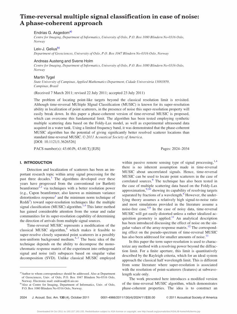
Consider separate or coincident source-receiver arrays
with Ns and Nr representing respectively the total number of
sources and receivers (cf. Figure 1). Each source generates a
time-varying wavefield, which propagates through the
known background medium with D embedded point scatter-
ers. It is further assumed that a temporal Fourier transform
has been applied to the transient data. Let the monochro-
matic signal vector s(x) (dimension Ns� 1) represent the
transmitted signal from the source array. Introduce now the
complex transfer Nr�Ns matrix, ~K(x), as follows (x repre-
senting the angular frequency):
~K xð Þ ¼ K xð Þ þ N xð Þ; (1)
where K(x) is the noise-free response matrix and N(x) rep-
resents the noise matrix. The monochromatic data associated
with this multi-source multi-receiver experiment can now be
written formally as
r xð Þ ¼ ~K xð Þ s xð Þ (2)
where r(x) represents the data measured at the receiver
array.
The noise-corrupted system matrix, ~K xð Þ, can be further
written on its SVD-form as11,13
~K xð Þ ¼ ~Usig xð Þ ~U? xð Þ� � ~Rsig xð Þ 0
0 ~R? xð Þ
" #~V
H
sig xð Þ
~VH
? xð Þ�
24
35
¼ ~Usig xð Þ~Rsig xð Þ ~VH
sig xð Þ þ ~U? xð Þ~R? xð Þ ~VH
? xð Þ; (3)
where the superscript H means complex-conjugated trans-
posed and the subscripts sig and \ represent the signal and
noise subspaces, respectively. In the noise-free case, Eq. (3)
simplifies to
K xð Þ ¼ Usig xð ÞU? xð Þ� � Rsig xð Þ 0
0 0
" #VH
sig xð Þ
VH? xð Þ�
" #
¼ Usig xð ÞRsig xð ÞVHsig xð Þ (4)
Here, Rsig¼ diag{rsig,1, rsig,2,., rsig,D}, is a diagonal matrix of
D non-zero, real singular values, corresponding to the scatterers.
Also, Usig¼ [usig,1…usig,D] and Vsig¼ [vsig,1…vsig,D], where
usig,i and vsig,i are (column) singular vectors of Usig and Vsig
corresponding to the singular values, rsig,i. It is assumed that
the rank of the matrix K is D<min(Ns, Nr), with D repre-
senting the total number of scatterers.7,11 In the same way,
the quantities R\, U\, and V\ represent the counterparts of
Rsig, Usig, and Vsig, associated to the noise subspace. We
finally have the orthonormality properties, namely,
UHsig xð ÞU? xð Þ ¼ 0;
VHsig xð ÞV? xð Þ ¼ 0;
(5)
which express the fact that the signal and noise (nil) subspa-
ces are orthogonal. Moreover,
UHsig xð ÞUsig xð Þ ¼ I;
VHsig xð ÞVsig xð Þ ¼ I;
(6)
and
UH? xð ÞU? xð Þ ¼ I;
VH? xð ÞV? xð Þ ¼ I;
(7)
which mean the singular vectors are normalized. Note that
we can recast Eq. (4) in the formFIG. 1. (Color online) Multi-source multi-receiver experiment involving a
cluster of D scatterers.
J. Acoust. Soc. Am., Vol. 130, No. 4, October 2011 Asgedom et al.: Time-reversal multiple signal classification 2025
Downloaded 04 Oct 2011 to 193.157.193.155. Redistribution subject to ASA license or copyright; see http://asadl.org/journals/doc/ASALIB-home/info/terms.jsp
K xð Þ ¼XD
i¼1
rsig;iKi xð Þ; (8)
with Ki ¼ usig;ivHsig;i: A multi-source experiment, where each
source is fired at separate times, generates incoherent signals
associated with the scatterers. This is due to the fact that each
source corresponds to a different location, resulting in varying
phases for each of the scattered signals. In addition, the struc-
ture of the response-matrix, K(x) (or ~K(x)) depends on the
actual type of acquisition geometry. In the case of moving
arrays like in seismic or ground penetrating radar (GPR) this
matrix will be partially filled, while for fixed-array ultrasound
acquisitions the matrix will be completely filled.
B. Incoherent time-reversal MUSIC algorithm
Assume now a noise-free experiment, which implies
that Eq. (4) is a valid representation. Further assume that the
scatterers are fully resolved (e.g., ideal array point-spread
functions with respect to both source and receiver side),
which mathematically can be stated as the conditions5,11
gH0r xi;xð Þg0r x;xð Þ ¼ g0r xi;xð Þk k2; if x ¼ xi;
0 if x 6¼ xi;
�(9a)
and
gH0s xi;xð Þg0s x;xð Þ ¼ g0s xi;xð Þk k2; if x ¼ xi;
0 if x 6¼ xi;
�(9b)
where gH0s xi;xð Þ and gH
0r xi;xð Þ represent monochromatic
background Green’s function (column) vectors with respect
to the source and receiver arrays that focus at a point scat-
terer located at the position xi, and x is the arbitrary test scat-
terer location. For well-resolved targets satisfying Eqs. (9a)
and (9b), an SVD of K(x) results in signal subspace singular
functions that are normalized versions of the Green’s func-
tion vectors associated with the scatterers.5,11 Thus, mathe-
matically the left- and right-singular matrices, Usig(x) and
Vsig(x), in Eq. (4) take the forms
Usig xð Þ ¼ g0r x1;xð Þg0r x1;xð Þk k eih1 ;
g0r x2;xð Þg0r x2;xð Þk k eih2 ;…;
g0r xD;xð Þg0r xD;xð Þk k eihD
� �;
Vsig xð Þ ¼ g�0s x1;xð Þg0s x1;xð Þk k eih1 ;
g�0s x2;xð Þg0s x2;xð Þk k eih2 ;…;
g�0s xD;xð Þg0s xD;xð Þk k eihD
� �;
(10)
where the superscript * denotes a complex conjugate. The
singular vectors output from an SVD analysis of a complex-
valued matrix system will be non-unique by an arbitrary
phase.11,14 The phase angles in Eqs. (10) represent symboli-
cally this non-uniqueness. Note, however, that the arbitrary
phase for the corresponding left- and right-singular vectors
are the same.
By using the orthogonality between the signal and noise
(nil) subspaces, a signal-subspace based MUSIC pseudo-
spectrum operator can be constructed as6,7,15
PMUSIC x;xð Þ ¼ 1
1� Ar x;xð Þ þ1
1� As x;xð Þ ; (11)
which will peak at the true target locations. In Eq. (11), Ar
and As represent the receiver and source normalized time-re-
versal operators
Ar x;xð Þ ¼ gH0r x;xð ÞPsig;r xð Þg0r x;xð Þ
gH0r x;xð Þg0r x;xð Þ ;
As x;xð Þ ¼ gT0s x;xð ÞPsig;s xð Þg�0s x;xð Þ
gT0s x;xð Þg�0s x;xð Þ ;
(12)
in which
Psig;r xð Þ ¼ Usig xð ÞUHsig xð Þ;
Psig;s xð Þ ¼ Vsig xð ÞVHsig xð Þ;
(13)
are the signal subspace projection matrices with respect to
receiver and source side, respectively. In the literature, the
signal-space based MUSIC pseudo-spectrum as given by Eq.
(11) is referred to as time-reversal MUSIC.7 It is to be
observed that the same terminology has also been used for a
nil-space based MUSIC algorithm.5 The reason is that the
SVD formulation transforms the passive target detection
problem into that of an active (secondary) source problem
associated with each scatterer.5,14,16 Time-reversal is an im-
portant concept that has been analyzed in detail in the litera-
ture (see, e.g., Ref. 7). A short summary of that concept and
its main properties is provided in Appendix A.
It is to be noted that the operators Ar(x, x) and As(x, x)
give magnitude values only. In a noise-free case both should
ideally be one at the location of the scatterer(s). If the data
are corrupted with noise the MUSIC pseudo-spectrum in Eq.
(11) takes the form
~PMUSIC x;xð Þ ¼ 1
1� ~Ar x;xð Þþ 1
1� ~As x;xð Þ; (14)
with the operation of time-reversal now being distorted by
noise and calculated according to the formulas
~Ar x;xð Þ ¼ gH0r x;xð Þ ~Psig;r xð Þg0r x;xð Þ
g0r x;xð Þk k2;
~As x;xð Þ ¼ gT0s x;xð Þ ~Psig;s xð Þg�0s x;xð Þ
g0s x;xð Þk k2;
(15)
2026 J. Acoust. Soc. Am., Vol. 130, No. 4, October 2011 Asgedom et al.: Time-reversal multiple signal classification
Downloaded 04 Oct 2011 to 193.157.193.155. Redistribution subject to ASA license or copyright; see http://asadl.org/journals/doc/ASALIB-home/info/terms.jsp
in which
~Psig;r xð Þ ¼ ~Usig xð Þ ~UHsig xð Þ;
~Psig;s xð Þ ¼ ~Vsig xð Þ ~VHsig xð Þ:
(16)
In the original time-reversal works,5–7 the issue of noise was
not discussed in detail. In the presence of noise, the distinc-
tion between the signal and nil subspaces is no longer per-
fectly defined. Hence, the two subspaces will start to mix
and the sharp border defined by the singular values will now
be replaced by a smooth transition zone. The effect of noise
on nil-subspace based time-reversal MUSIC has been previ-
ously analyzed employing a linearized perturbation theory.11
Applying a similar approach here, gives the following
expected values of the time-reversal operations in Eqs. (15)
[cf. Eqs. (B11), (B13), and (B14) in Appendix B]
E ~Ar x;xð Þ� �
¼ Ar x;xð Þ þ fr2A?;r x;xð Þ;E ~As x;xð Þ� �
¼ As x;xð Þ þ fr2A?;s x;xð Þ;(17)
where
A?;r x;xð Þ ¼ gH0r x;xð ÞP?;r xð Þg0r x;xð Þ
g0r x;xð Þk k2;
A?;s x;xð Þ ¼ gT0s x;xð ÞP?;s xð Þg�0s x;xð Þ
g0s x;xð Þk k2;
(18)
in which
P?;r xð Þ ¼ U? xð ÞUH? xð Þ;
P?;s xð Þ ¼ V? xð ÞVH? xð Þ; (19)
are the receiver and source projection matrices of the nil-
subspace (noise-free case). Moreover, r2 is the variance of
the noise (assuming a variance of r2/2 of both real and imag-
inary parts of the noise matrix N) and
f ¼ 1
r2sig;1
þ 1
r2sig;2
þ :::þ 1
r2sig;D
: (20)
It follows directly from Eqs. (17) that, at each scatterer loca-
tion, the expected values of the time-reversal operations will
be the same as for the noise-free case (unit value and no
phase). This implies also that the (noise) time-reversal
MUSIC operator in Eq. (14) will have the same expectation
value as in the noise-free case at each scatterer location
(within a linearized noise model). This will apply for every
frequency considered.
For a given frequency band, Dx, the multi-frequency
equivalent of Eqs. (14) and (17) can be introduced (Nx rep-
resenting the number of discrete frequencies available),
namely,
~PMUSIC x;Dxð Þ ¼ 1
1� ~Ar x;Dxð Þþ 1
1� ~As x;Dxð Þ; (21)
where
~Ar x;Dxð Þ ¼ 1
Nx
XDx
~Ar x;xð Þ;
~As x;Dxð Þ ¼ 1
Nx
XDx
~As x;xð Þ:(22)
However, these quantities contain no phase information.
Hence, in the case of noise, they will not coherently add at the
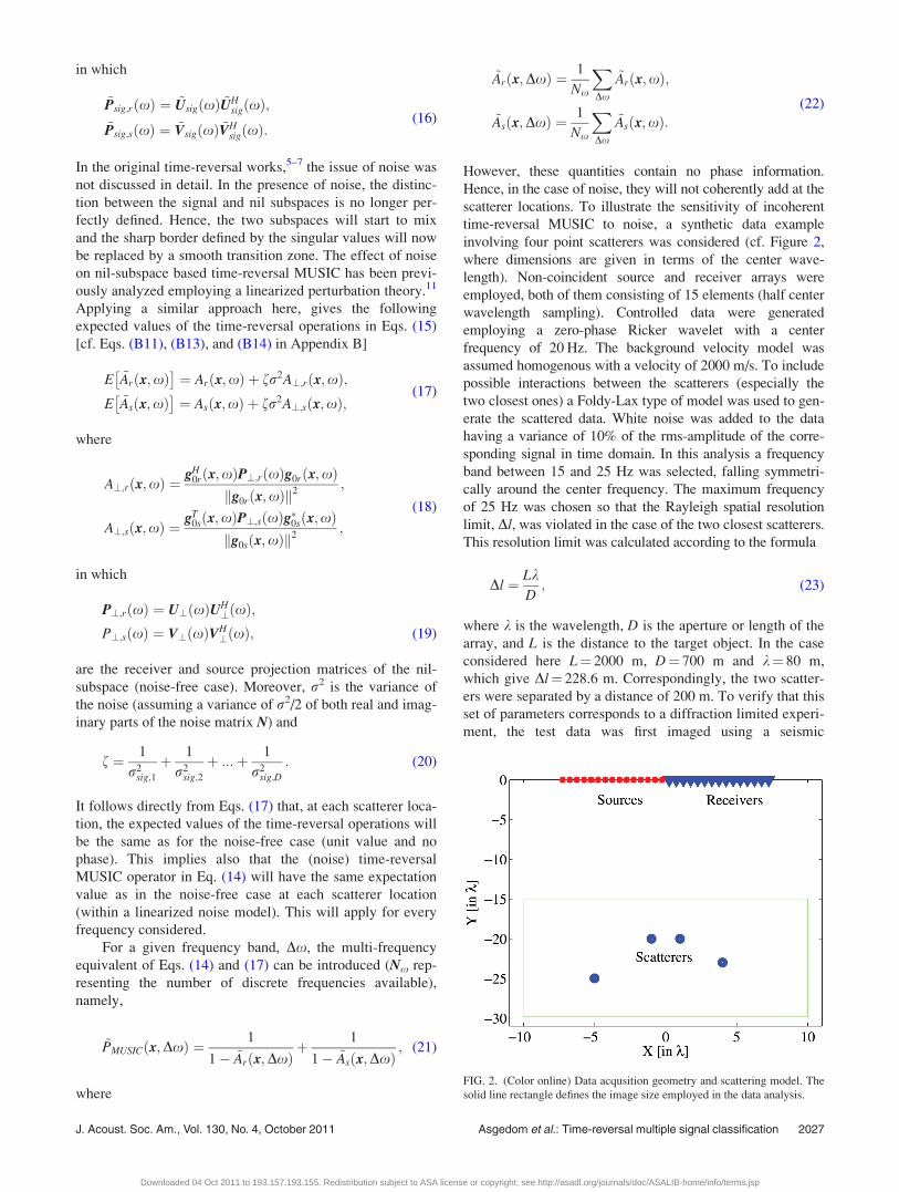
scatterer locations. To illustrate the sensitivity of incoherent
time-reversal MUSIC to noise, a synthetic data example
involving four point scatterers was considered (cf. Figure 2,
where dimensions are given in terms of the center wave-
length). Non-coincident source and receiver arrays were
employed, both of them consisting of 15 elements (half center
wavelength sampling). Controlled data were generated
employing a zero-phase Ricker wavelet with a center
frequency of 20 Hz. The background velocity model was
assumed homogenous with a velocity of 2000 m/s. To include
possible interactions between the scatterers (especially the
two closest ones) a Foldy-Lax type of model was used to gen-
erate the scattered data. White noise was added to the data
having a variance of 10% of the rms-amplitude of the corre-
sponding signal in time domain. In this analysis a frequency
band between 15 and 25 Hz was selected, falling symmetri-
cally around the center frequency. The maximum frequency
of 25 Hz was chosen so that the Rayleigh spatial resolution
limit, Dl, was violated in the case of the two closest scatterers.
This resolution limit was calculated according to the formula
Dl ¼ LkD; (23)
where k is the wavelength, D is the aperture or length of the
array, and L is the distance to the target object. In the case
considered here L¼ 2000 m, D¼ 700 m and k¼ 80 m,
which give Dl¼ 228.6 m. Correspondingly, the two scatter-
ers were separated by a distance of 200 m. To verify that this
set of parameters corresponds to a diffraction limited experi-
ment, the test data was first imaged using a seismic
FIG. 2. (Color online) Data acqusition geometry and scattering model. The
solid line rectangle defines the image size employed in the data analysis.
J. Acoust. Soc. Am., Vol. 130, No. 4, October 2011 Asgedom et al.: Time-reversal multiple signal classification 2027
Downloaded 04 Oct 2011 to 193.157.193.155. Redistribution subject to ASA license or copyright; see http://asadl.org/journals/doc/ASALIB-home/info/terms.jsp
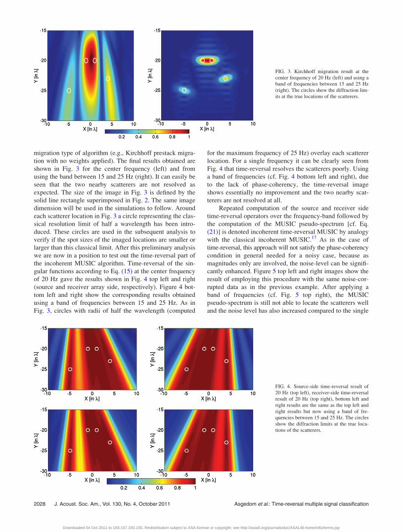
migration type of algorithm (e.g., Kirchhoff prestack migra-
tion with no weights applied). The final results obtained are
shown in Fig. 3 for the center frequency (left) and from
using the band between 15 and 25 Hz (right). It can easily be
seen that the two nearby scatterers are not resolved as
expected. The size of the image in Fig. 3 is defined by the
solid line rectangle superimposed in Fig. 2. The same image
dimension will be used in the simulations to follow. Around
each scatterer location in Fig. 3 a circle representing the clas-
sical resolution limit of half a wavelength has been intro-
duced. These circles are used in the subsequent analysis to
verify if the spot sizes of the imaged locations are smaller or
larger than this classical limit. After this preliminary analysis
we are now in a position to test out the time-reversal part of
the incoherent MUSIC algorithm. Time-reversal of the sin-
gular functions according to Eq. (15) at the center frequency
of 20 Hz gave the results shown in Fig. 4 top left and right
(source and receiver array side, respectively). Figure 4 bot-
tom left and right show the corresponding results obtained
using a band of frequencies between 15 and 25 Hz. As in
Fig. 3, circles with radii of half the wavelength (computed
for the maximum frequency of 25 Hz) overlay each scatterer
location. For a single frequency it can be clearly seen from
Fig. 4 that time-reversal resolves the scatterers poorly. Using
a band of frequencies (cf. Fig. 4 bottom left and right), due
to the lack of phase-coherency, the time-reversal image
shows essentially no improvement and the two nearby scat-
terers are not resolved at all.
Repeated computation of the source and receiver side
time-reversal operators over the frequency-band followed by
the computation of the MUSIC pseudo-spectrum [cf. Eq.
(21)] is denoted incoherent time-reversal MUSIC by analogy
with the classical incoherent MUSIC.17 As in the case of
time-reversal, this approach will not satisfy the phase-coherency
condition in general needed for a noisy case, because as
magnitudes only are involved, the noise-level can be signifi-
cantly enhanced. Figure 5 top left and right images show the
result of employing this procedure with the same noise-cor-
rupted data as in the previous example. After applying a
band of frequencies (cf. Fig. 5 top right), the MUSIC
pseudo-spectrum is still not able to locate the scatterers well
and the noise level has also increased compared to the single
FIG. 3. Kirchhoff migration result at the
center frequency of 20 Hz (left) and using a
band of frequencies between 15 and 25 Hz
(right). The circles show the diffraction lim-
its at the true locations of the scatterers.
FIG. 4. Source-side time-reversal result of
20 Hz (top left), receiver-side time-reversal
result of 20 Hz (top right), bottom left and
right results are the same as the top left and
right results but now using a band of fre-
quencies between 15 and 25 Hz. The circles
show the diffraction limits at the true loca-
tions of the scatterers.
2028 J. Acoust. Soc. Am., Vol. 130, No. 4, October 2011 Asgedom et al.: Time-reversal multiple signal classification
Downloaded 04 Oct 2011 to 193.157.193.155. Redistribution subject to ASA license or copyright; see http://asadl.org/journals/doc/ASALIB-home/info/terms.jsp
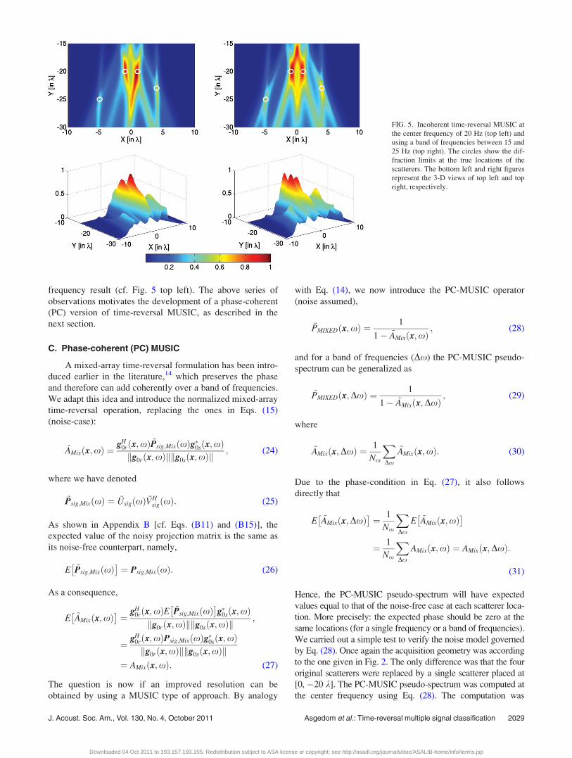
frequency result (cf. Fig. 5 top left). The above series of
observations motivates the development of a phase-coherent
(PC) version of time-reversal MUSIC, as described in the
next section.
C. Phase-coherent (PC) MUSIC
A mixed-array time-reversal formulation has been intro-
duced earlier in the literature,14 which preserves the phase
and therefore can add coherently over a band of frequencies.
We adapt this idea and introduce the normalized mixed-array
time-reversal operation, replacing the ones in Eqs. (15)
(noise-case):
~AMix x;xð Þ ¼ gH0r x;xð Þ ~Psig;Mix xð Þg�0s x;xð Þ
g0r x;xð Þk k g0s x;xð Þk k ; (24)
where we have denoted
~Psig;Mix xð Þ ¼ ~Usig xð Þ ~VHsig xð Þ: (25)
As shown in Appendix B [cf. Eqs. (B11) and (B15)], the
expected value of the noisy projection matrix is the same as
its noise-free counterpart, namely,
E ~Psig;Mix xð Þ� �
¼ Psig;Mix xð Þ: (26)
As a consequence,
E ~AMix x;xð Þ� �
¼gH
0r x;xð ÞE ~Psig;Mix xð Þ� �
g�0s x;xð Þg0r x;xð Þk k g0s x;xð Þk k ;
¼ gH0r x;xð ÞPsig;Mix xð Þg�0s x;xð Þ
g0r x;xð Þk k g0s x;xð Þk k¼ AMix x;xð Þ: (27)
The question is now if an improved resolution can be
obtained by using a MUSIC type of approach. By analogy
with Eq. (14), we now introduce the PC-MUSIC operator
(noise assumed),
~PMIXED x;xð Þ ¼ 1
1� ~AMix x;xð Þ; (28)
and for a band of frequencies (Dx) the PC-MUSIC pseudo-
spectrum can be generalized as
~PMIXED x;Dxð Þ ¼ 1
1� ~AMix x;Dxð Þ; (29)
where
~AMix x;Dxð Þ ¼ 1
Nx
XDx
~AMix x;xð Þ: (30)
Due to the phase-condition in Eq. (27), it also follows
directly that
E ~AMix x;Dxð Þ� �
¼ 1
Nx
XDx
E ~AMix x;xð Þ� �
¼ 1
Nx
XDx
AMix x;xð Þ ¼ AMix x;Dxð Þ:
(31)
Hence, the PC-MUSIC pseudo-spectrum will have expected
values equal to that of the noise-free case at each scatterer loca-
tion. More precisely: the expected phase should be zero at the
same locations (for a single frequency or a band of frequencies).
We carried out a simple test to verify the noise model governed
by Eq. (28). Once again the acquisition geometry was according
to the one given in Fig. 2. The only difference was that the four
original scatterers were replaced by a single scatterer placed at
[0, �20 k]. The PC-MUSIC pseudo-spectrum was computed at
the center frequency using Eq. (28). The computation was
FIG. 5. Incoherent time-reversal MUSIC at
the center frequency of 20 Hz (top left) and
using a band of frequencies between 15 and
25 Hz (top right). The circles show the dif-
fraction limits at the true locations of the
scatterers. The bottom left and right figures
represent the 3-D views of top left and top
right, respectively.
J. Acoust. Soc. Am., Vol. 130, No. 4, October 2011 Asgedom et al.: Time-reversal multiple signal classification 2029
Downloaded 04 Oct 2011 to 193.157.193.155. Redistribution subject to ASA license or copyright; see http://asadl.org/journals/doc/ASALIB-home/info/terms.jsp
repeated 81 times and each time white noise was added to
the signal before SVD (variance of noise about 10% of rms-
amplitude of signal in time-domain). For each computation the
phase of the pseudo-spectrum at the exact scatterer location was
extracted. Figure 6 top shows how this phase varies in a random
manner for this ensemble of experiments. In addition, the indi-
vidual pseudo-spectra were added together and the phase of this
PC-MUSIC operator was calculated again at the scatterer point
(shown as a solid curve in Fig. 6 top). As expected, the phase of
the PC-MUSIC operator is now close to zero at the target loca-
tion [as predicted from Eqs. (27) and (28)].
The time-reversal part of the PC-MUSIC operator in Eq.
(29) has the phase-coherency property sought after.14 It is
therefore likely to expect that PC-MUSIC also shows the
same property. More specifically, its pseudo-spectrum should
have a phase close to zero at each scatterer location after fre-
quency summation. This is also supported by the results
obtained in Fig. 6 top. Because the random phase behavior
observed in this figure will occur for every available fre-
quency, the phase variation with frequency will consequently
also vary randomly at the location of a scatterer. To verify
this assumption we repeated the previous experiment except
with one change: Instead of varying the number of experi-
ments for a fixed frequency we varied the frequency by scan-
ning through the defined band (same as before). For each
individual frequency the phase of the pseudo-spectrum was
computed at the target location. Finally, each pseudo-spectrum
was added based on Eq. (29) to demonstrate the inherent
phase-coherency characteristic. The results are summarized
in Fig. 6 bottom. It can easily be seen that the phase is close
to zero (solid curve) after frequency-summation.
After having carefully analyzed the characteristics of
the proposed PC-MUSIC operator, it is time to compare its
performance with that of incoherent time-reversal MUSIC.
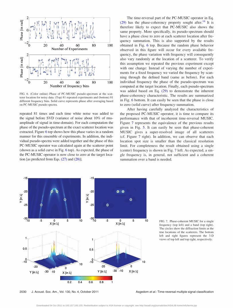
Figure 7 represents the equivalence of the previous results
given in Fig. 5. It can easily be seen that phase-coherent
MUSIC gives a super-resolved image of all scatterers
(cf. Figure 7 right). In addition, we can observe that each
location spot size is smaller than the classical resolution
limit. For completeness the result obtained using a single
(center) frequency is shown in Fig. 7 left. As expected, a sin-
gle frequency is, in general, not sufficient and a coherent
summation over a band is needed.
FIG. 6. (Color online) Phase of PC-MUSIC pseudo-spectrum at the scat-
terer location for noisy data. (Top) 81 repeated experiments and (bottom) 81
different frequency bins. Solid curve represents phase after averaging based
on PC-MUSIC pseudo-spectra.
FIG. 7. Phase-coherent MUSIC for a single
frequency (top left) and a band (top right).
The circles show the diffraction limits at the
true locations of the scatterers. The bottom
left and right figures represent the 3-D
views of top left and top right, respectively.
2030 J. Acoust. Soc. Am., Vol. 130, No. 4, October 2011 Asgedom et al.: Time-reversal multiple signal classification
Downloaded 04 Oct 2011 to 193.157.193.155. Redistribution subject to ASA license or copyright; see http://asadl.org/journals/doc/ASALIB-home/info/terms.jsp
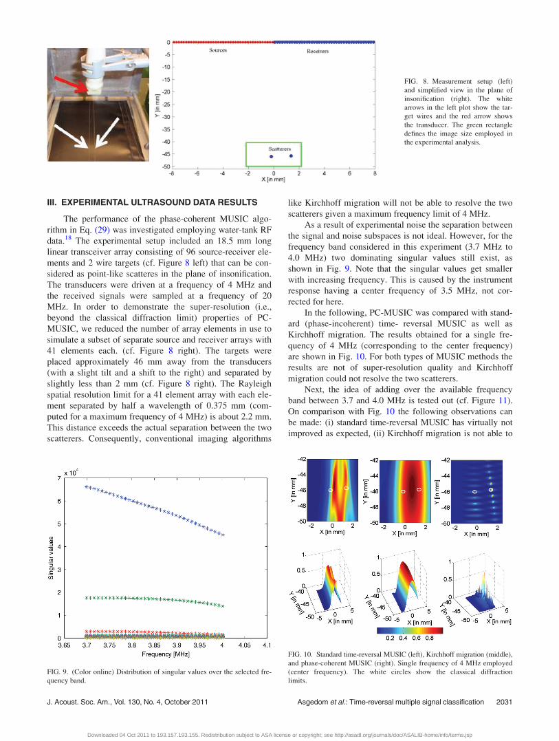
III. EXPERIMENTAL ULTRASOUND DATA RESULTS
The performance of the phase-coherent MUSIC algo-
rithm in Eq. (29) was investigated employing water-tank RF
data.18 The experimental setup included an 18.5 mm long
linear transceiver array consisting of 96 source-receiver ele-
ments and 2 wire targets (cf. Figure 8 left) that can be con-
sidered as point-like scatteres in the plane of insonification.
The transducers were driven at a frequency of 4 MHz and
the received signals were sampled at a frequency of 20
MHz. In order to demonstrate the super-resolution (i.e.,
beyond the classical diffraction limit) properties of PC-
MUSIC, we reduced the number of array elements in use to
simulate a subset of separate source and receiver arrays with
41 elements each. (cf. Figure 8 right). The targets were
placed approximately 46 mm away from the transducers
(with a slight tilt and a shift to the right) and separated by
slightly less than 2 mm (cf. Figure 8 right). The Rayleigh
spatial resolution limit for a 41 element array with each ele-
ment separated by half a wavelength of 0.375 mm (com-
puted for a maximum frequency of 4 MHz) is about 2.2 mm.
This distance exceeds the actual separation between the two
scatterers. Consequently, conventional imaging algorithms
like Kirchhoff migration will not be able to resolve the two
scatterers given a maximum frequency limit of 4 MHz.
As a result of experimental noise the separation between
the signal and noise subspaces is not ideal. However, for the
frequency band considered in this experiment (3.7 MHz to
4.0 MHz) two dominating singular values still exist, as
shown in Fig. 9. Note that the singular values get smaller
with increasing frequency. This is caused by the instrument
response having a center frequency of 3.5 MHz, not cor-
rected for here.
In the following, PC-MUSIC was compared with stand-
ard (phase-incoherent) time- reversal MUSIC as well as
Kirchhoff migration. The results obtained for a single fre-
quency of 4 MHz (corresponding to the center frequency)
are shown in Fig. 10. For both types of MUSIC methods the
results are not of super-resolution quality and Kirchhoff
migration could not resolve the two scatterers.
Next, the idea of adding over the available frequency
band between 3.7 and 4.0 MHz is tested out (cf. Figure 11).
On comparison with Fig. 10 the following observations can
be made: (i) standard time-reversal MUSIC has virtually not
improved as expected, (ii) Kirchhoff migration is not able to
FIG. 8. Measurement setup (left)
and simplified view in the plane of
insonification (right). The white
arrows in the left plot show the tar-
get wires and the red arrow shows
the transducer. The green rectangle
defines the image size employed in
the experimental analysis.
FIG. 9. (Color online) Distribution of singular values over the selected fre-
quency band.
FIG. 10. Standard time-reversal MUSIC (left), Kirchhoff migration (middle),
and phase-coherent MUSIC (right). Single frequency of 4 MHz employed
(center frequency). The white circles show the classical diffraction
limits.
J. Acoust. Soc. Am., Vol. 130, No. 4, October 2011 Asgedom et al.: Time-reversal multiple signal classification 2031
Downloaded 04 Oct 2011 to 193.157.193.155. Redistribution subject to ASA license or copyright; see http://asadl.org/journals/doc/ASALIB-home/info/terms.jsp
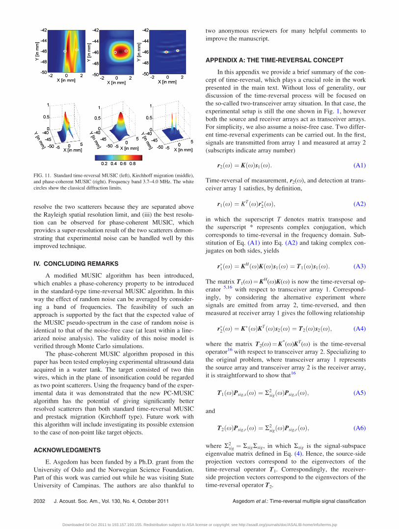
resolve the two scatterers because they are separated above
the Rayleigh spatial resolution limit, and (iii) the best resolu-
tion can be observed for phase-coherent MUSIC, which
provides a super-resolution result of the two scatterers demon-
strating that experimental noise can be handled well by this
improved technique.
IV. CONCLUDING REMARKS
A modified MUSIC algorithm has been introduced,
which enables a phase-coherency property to be introduced
in the standard-type time-reversal MUSIC algorithm. In this
way the effect of random noise can be averaged by consider-
ing a band of frequencies. The feasibility of such an
approach is supported by the fact that the expected value of
the MUSIC pseudo-spectrum in the case of random noise is
identical to that of the noise-free case (at least within a line-
arized noise analysis). The validity of this noise model is
verified through Monte Carlo simulations.
The phase-coherent MUSIC algorithm proposed in this
paper has been tested employing experimental ultrasound data
acquired in a water tank. The target consisted of two thin
wires, which in the plane of insonification could be regarded
as two point scatterers. Using the frequency band of the exper-
imental data it was demonstrated that the new PC-MUSIC
algorithm has the potential of giving significantly better
resolved scatterers than both standard time-reversal MUSIC
and prestack migration (Kirchhoff type). Future work with
this algorithm will include investigating its possible extension
to the case of non-point like target objects.
ACKNOWLEDGMENTS
E. Asgedom has been funded by a Ph.D. grant from the
University of Oslo and the Norwegian Science Foundation.
Part of this work was carried out while he was visiting State
University of Campinas. The authors are also thankful to
two anonymous reviewers for many helpful comments to
improve the manuscript.
APPENDIX A: THE TIME-REVERSAL CONCEPT
In this appendix we provide a brief summary of the con-
cept of time-reversal, which plays a crucial role in the work
presented in the main text. Without loss of generality, our
discussion of the time-reversal process will be focused on
the so-called two-transceiver array situation. In that case, the
experimental setup is still the one shown in Fig. 1, however
both the source and receiver arrays act as transceiver arrays.
For simplicity, we also assume a noise-free case. Two differ-
ent time-reversal experiments can be carried out. In the first,
signals are transmitted from array 1 and measured at array 2
(subscripts indicate array number)
r2 xð Þ ¼ K xð Þs1 xð Þ: (A1)
Time-reversal of measurement, r2(x), and detection at trans-
ceiver array 1 satisfies, by definition,
r1 xð Þ ¼ KT xð Þr�2 xð Þ; (A2)
in which the superscript T denotes matrix transpose and
the superscript * represents complex conjugation, which
corresponds to time-reversal in the frequency domain. Sub-
stitution of Eq. (A1) into Eq. (A2) and taking complex con-
jugates on both sides, yields
r�1 xð Þ ¼ KH xð ÞK xð Þs1 xð Þ ¼ T1 xð Þs1 xð Þ: (A3)
The matrix T1(x)¼KH(x)K(x) is now the time-reversal op-
erator 5,16 with respect to transceiver array 1. Correspond-
ingly, by considering the alternative experiment where
signals are emitted from array 2, time-reversed, and then
measured at receiver array 1 gives the following relationship
r�2 xð Þ ¼ K� xð ÞKT xð Þs2 xð Þ ¼ T2 xð Þs2 xð Þ; (A4)
where the matrix T2(x)¼K*(x)KT(x) is the time-reversal
operator16 with respect to transceiver array 2. Specializing to
the original problem, where transceiver array 1 represents
the source array and transceiver array 2 is the receiver array,
it is straightforward to show that16
T1 xð ÞPsig;s xð Þ ¼ R2sig xð ÞPsig;s xð Þ; (A5)
and
T2 xð ÞPsig;r xð Þ ¼ R2sig xð ÞPsig;r xð Þ; (A6)
where R2sig ¼ RsigRsig, in which Rsig is the signal-subspace
eigenvalue matrix defined in Eq. (4). Hence, the source-side
projection vectors correspond to the eigenvectors of the
time-reversal operator T1. Correspondingly, the receiver-
side projection vectors correspond to the eigenvectors of the
time-reversal operator T2.
FIG. 11. Standard time-reversal MUSIC (left), Kirchhoff migration (middle),
and phase-coherent MUSIC (right). Frequency band 3.7–4.0 MHz. The white
circles show the classical diffraction limits.
2032 J. Acoust. Soc. Am., Vol. 130, No. 4, October 2011 Asgedom et al.: Time-reversal multiple signal classification
Downloaded 04 Oct 2011 to 193.157.193.155. Redistribution subject to ASA license or copyright; see http://asadl.org/journals/doc/ASALIB-home/info/terms.jsp
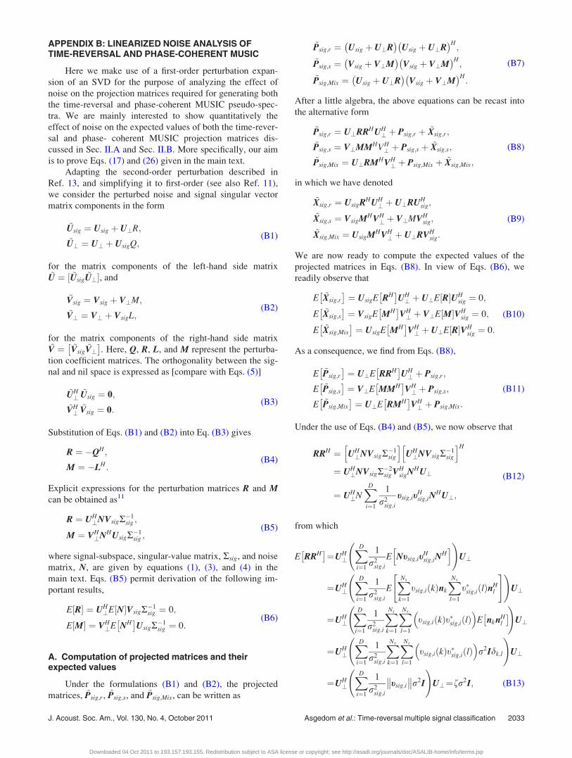
APPENDIX B: LINEARIZED NOISE ANALYSIS OFTIME-REVERSAL AND PHASE-COHERENT MUSIC
Here we make use of a first-order perturbation expan-
sion of an SVD for the purpose of analyzing the effect of
noise on the projection matrices required for generating both
the time-reversal and phase-coherent MUSIC pseudo-spec-
tra. We are mainly interested to show quantitatively the
effect of noise on the expected values of both the time-rever-
sal and phase- coherent MUSIC projection matrices dis-
cussed in Sec. II.A and Sec. II.B. More specifically, our aim
is to prove Eqs. (17) and (26) given in the main text.
Adapting the second-order perturbation described in
Ref. 13, and simplifying it to first-order (see also Ref. 11),
we consider the perturbed noise and signal singular vector
matrix components in the form
~Usig ¼ Usig þ U?R;
~U? ¼ U? þ UsigQ;(B1)
for the matrix components of the left-hand side matrix~U ¼ ½ ~Usig
~U?�, and
~Vsig ¼ Vsig þ V?M;
~V? ¼ V? þ VsigL;(B2)
for the matrix components of the right-hand side matrix~V ¼ ~Vsig
~V?� �
. Here, Q, R, L, and M represent the perturba-
tion coefficient matrices. The orthogonality between the sig-
nal and nil space is expressed as [compare with Eqs. (5)]
~UH? ~Usig ¼ 0;
~VH?
~Vsig ¼ 0:(B3)
Substitution of Eqs. (B1) and (B2) into Eq. (B3) gives
R ¼ �QH;
M ¼ �LH:(B4)
Explicit expressions for the perturbation matrices R and Mcan be obtained as11
R ¼ UH?NVsigR
�1sig ;
M ¼ VH?NHUsigR
�1sig ;
(B5)
where signal-subspace, singular-value matrix, Rsig, and noise
matrix, N, are given by equations (1), (3), and (4) in the
main text. Eqs. (B5) permit derivation of the following im-
portant results,
E R½ � ¼ UH?E N½ �VsigR
�1sig ¼ 0;
E M½ � ¼ VH?E NH� �
UsigR�1sig ¼ 0:
(B6)
A. Computation of projected matrices and theirexpected values
Under the formulations (B1) and (B2), the projected
matrices, ~Psig;r, ~Psig;s, and ~Psig;Mix, can be written as
~Psig;r ¼ Usig þ U?R� �
Usig þ U?R� �H
;
~Psig;s ¼ Vsig þ V?M� �
Vsig þ V?M� �H
;
~Psig;Mix ¼ Usig þ U?R� �
Vsig þ V?M� �H
:
(B7)
After a little algebra, the above equations can be recast into
the alternative form
~Psig;r ¼ U?RRHUH? þ Psig;r þ ~Xsig;r;
~Psig;s ¼ V?MMHVH? þ Psig;s þ ~Xsig;s;
~Psig;Mix ¼ U?RMHVH? þ Psig;Mix þ ~Xsig;Mix;
(B8)
in which we have denoted
~Xsig;r ¼ UsigRHUH? þ U?RUH
sig;
~Xsig;s ¼ VsigMHVH? þ V?MVH
sig;
~Xsig;Mix ¼ UsigMHVH? þ U?RVH
sig:
(B9)
We are now ready to compute the expected values of the
projected matrices in Eqs. (B8). In view of Eqs. (B6), we
readily observe that
E ~Xsig;r
� �¼ UsigE RH
� �UH? þ U?E R½ �UH
sig ¼ 0;
E ~Xsig;s
� �¼ VsigE MH
� �VH? þ V?E M½ �VH
sig ¼ 0;
E ~Xsig;Mix
� �¼ UsigE MH
� �VH? þ U?E R½ �VH
sig ¼ 0:
(B10)
As a consequence, we find from Eqs. (B8),
E ~Psig;r
� �¼ U?E RRH
� �UH? þ Psig;r;
E ~Psig;s
� �¼ V?E MMH
� �VH? þ Psig;s;
E ~Psig;Mix
� �¼ U?E RMH
� �VH? þ Psig;Mix:
(B11)
Under the use of Eqs. (B4) and (B5), we now observe that
RRH ¼ UH?NVsigR
�1sig
h iUH?NVsigR
�1sig
h iH
¼ UH?NVsigR
�2sig VH
sigNHU?
¼ UH?NXD
i¼1
1
r2sig;i
tsig;itHsig;iN
HU?;
(B12)
from which
E RRH� �
¼UH?XD
i¼1
1
r2sig;i
E Ntsig;itHsig;iN
Hh i !
U?
¼UH?XD
i¼1
1
r2sig;i
EXNs
k¼1
tsig;i kð Þnk
XNs
l¼1
t�sig;i lð ÞnHl
" # !U?
¼UH?XD
i¼1
1
r2sig;i
XNs
k¼1
XNs
l¼1
tsig;i kð Þt�sig;i lð Þ
E nknHl
� � !U?
¼UH?XD
i¼1
1
r2sig;i
XNs
k¼1
XNs
l¼1
tsig;i kð Þt�sig;i lð Þ
r2Idk;l
!U?
¼UH?XD
i¼1
1
r2sig;i
tsig;i
�� ��r2I
!U?¼fr2I; (B13)
J. Acoust. Soc. Am., Vol. 130, No. 4, October 2011 Asgedom et al.: Time-reversal multiple signal classification 2033
Downloaded 04 Oct 2011 to 193.157.193.155. Redistribution subject to ASA license or copyright; see http://asadl.org/journals/doc/ASALIB-home/info/terms.jsp
where tsig,i(k) represents the k-th element of the vector tsig,i,
t�sig;i(l) represents the l-th element of the vector tHsig;i, nk is
the k-th column vector of N, nl is the l-th row vector of NH,
and f is given by Eq. (20). In the same way, we have
E MMH� �
¼ VH?XD
i¼1
1
r2sig;i
E NHusig;iuHsig;iN
h i !V?
¼ fr2I; (B14)
and the same approach gives also
E RMH� �
¼UH?XD
i¼1
1
r2sig;i
E Ntsig;iuHsig;iN
h i !V?
¼UH?XD
i¼1
1
r2sig;i
EXNs
k¼1
tsig;i kð Þnk
XNr
l¼1
u�sig;i lð Þnl
" # !V?
¼UH?XD
i¼1
1
r2sig;i
XNs
k¼1
XNr
l¼1
tsig;i kð Þu�sig;i lð ÞE nknl½ � !
V?
¼ 0; (B15)
where nl is the l-th row vector of N. Finally, using Eqs.
(B11) and (B13)–(B15), we readily recover Eqs. (17) and
(26) in the main text.
1H. Krim and M. Viberg, “Two decades of array signal processing
research,” IEEE Signal Process. Mag., 47, 67–94 (1996).2M. S. Bartlett, “Smoothing periodograms from time series with continuous
spectra,” Nature 161, 686–687 (1948).3S. S. Reddi, “Multiple source locationa digital approach,” IEEE Trans.
Aerosp. Electron. Syst., 15, 95–105 (1979).
4R. O. Schmidt, “Multiple emitter location and signal parameter
estimation,” IEEE Trans. Antennas Propag. 34, 276–280 (1986).5S. K. Lehman and A. J. Devaney, “Transmission mode time-reversal
super-resolution imaging,” J. Acoust. Soc. Am. 113, 2742–2753 (2003).6C. Prada and J. L. Thomas, “Experimental subwavelength localization of
scatterers by decomposition of the time reversal operator interpreted as a
covariance matrix,” J. Acoust. Soc. Am. 114, 235–243 (2003).7A. J. Devaney, “Super-resolution processing of multi-static data using
time-reversal and MUSIC,” Northeastern University Report, available at
http://www.ece.neu.edu/faculty/ devaney/ajd/preprints.htm (Last viewed
February 10, 2011).8A. J. Devaney, “Time reversal imaging of obscured targets from multi-
static data,” IEEE Trans Antennas Propag. 53, 1600–1610 (2005).9F. K. Gruber, E. A. Marengo, and A. J. Devaney, “Time-reversal imaging
with multiple signal classification considering multiple scattering between
the targets,” J. Acoust. Soc. Am. 115, 3042–3047 (2004).10F. Simonetti, M. Fleming, and E. A. Marengo, “Illustration of the role of
multiple scattering in subwavelength imaging from far-field meas-
urements,” J. Opt. Soc. Am. 25, 292–303 (2008).11L.-J. Gelius and E. G. Asgedom, “Diffraction-limited imaging and beyond -
the concept of super resolution,” Geophys. Prospect. 59, 400–421 (2010).12M. Davy, J.-G. Minonzio, J. de Rosny, C. Prada, and M. Fink, “Influence
of noise on subwavelength imaging of two close scatterers using time re-
versal method: theory and experiments,” Prog. Electromagn. Res. 98,
333–358 (2009).13R. J. Vaccaro, “A second-order perturbation expansion for the SVD,”
SIAM J. Matrix Anal. Appl. 15, 661–671 (1994).14S. Hou, K. Huang, K. Solna, and H. Zhao, “A phase and space coherent
direct imaging method,” J. Acoust. Soc. Am. 25, 227–238 (2009).15S. Hou, K. Solna, and H. Zhao, “A direct imaging method using far field
data,” Inverse Probl. 23, 1533–1546 (2007).16L.-J. Gelius, “Time-reversal and super-resolution in case of two trans-
ceiver arrays: Generalized DORT,” in Proceedings of the CPS/SEGBeijing International Conference and Exposition, April 24–27, Beijing,
China (2009).17H. Wang and M. Kaveh, “Coherent signal-subspace processing for the detec-
tion and estimation of angles of arrival of multiple wide-band sources,”
IEEE Trans. Acoust., Speech, Signal Process. 33, 823–831 (1985).18J.-F. Synnevag, A. Austeng, and S. Holm, “Adaptive beamforming applied
to medical ultrasound imaging,” IEEE Trans. Ultrason. Ferroelectr. Freq.
Control, 54, 1606–1613 (2007).
2034 J. Acoust. Soc. Am., Vol. 130, No. 4, October 2011 Asgedom et al.: Time-reversal multiple signal classification
Downloaded 04 Oct 2011 to 193.157.193.155. Redistribution subject to ASA license or copyright; see http://asadl.org/journals/doc/ASALIB-home/info/terms.jsp


