
Three Dimensional Analysis of Pier Extension and Guide Wall Design Alternatives to Mitigate Local Scour Risk at the BNSF Railroad Bridge Downstream of the Prado Dam
March 2015
ANL/ESD-15/7

Disclaimer This report was prepared as an account of work sponsored by an agency of the United States Government. Neither the United States Government nor any agency thereof, nor UChicago Argonne, LLC, nor any of their employees or officers, makes any warranty, express or implied, or assumes any legal liability or responsibility for the accuracy, completeness, or usefulness of any information, apparatus, product, or process disclosed, or represents that its use would not infringe privately owned rights. Reference herein to any specific commercial product, process, or service by trade name, trademark, manufacturer, or otherwise, does not necessarily constitute or imply its endorsement, recommendation, or favoring by the United States Government or any agency thereof. The views and opinions of document authors expressed herein do not necessarily state or reflect those of the United States Government or any agency thereof, Argonne National Laboratory, or UChicago Argonne, LLC.
DOCUMENT AVAILABILITY Online Access: U.S. Department of Energy (DOE) reports produced after 1991 and a growing number of pre-1991 documents are available free via DOE’s SciTech Connect (http://www.osti.gov/scitech/) Reports not in digital format may be purchased by the public from the National Technical Information Service (NTIS): U.S. Department of Commerce National Technical Information Service 5301 Shawnee Rd Alexandra, VA 22312 www.ntis.gov Phone: (800) 553-NTIS (6847) or (703) 605-6000 Fax: (703) 605-6900 Email: [email protected] Reports not in digital format are available to DOE and DOE contractors from the Office of Scientific and Technical Information (OSTI): U.S. Department of Energy Office of Scientific and Technical Information P.O. Box 62 Oak Ridge, TN 37831-0062 www.osti.gov Phone: (865) 576-8401 Fax: (865) 576-5728 Email: [email protected]
About Argonne National Laboratory
Argonne is a U.S. Department of Energy laboratory managed by UChicago Argonne, LLC
under contract DE-AC02-06CH11357. The Laboratory’s main facility is outside Chicago, at
9700 South Cass Avenue, Argonne, Illinois 60439. For information about Argonne and its
pioneering science and technology programs, see www.anl.gov.

Three Dimensional Analysis of Pier Extension
and Guide Wall Design Alternatives to Mitigate
Local Scour Risk at the BNSF Railroad Bridge
Downstream of the Prado Dam
by
S.A. Lottes, N. Sinha, and C. Bojanowski
Transportation Research and Analysis Computing Center (TRACC)
Energy Systems Division, Argonne National Laboratory
K. Kerenyi
Turner-Fairbank Highway Research Center
Federal Highway Administration
U.S. Department of Transportation
March 2015
ANL/ESD-15/7
TRACC/BNSF Bridge Scour Countermeasure Analysis Page I
Table of Contents
1. Introduction and Objectives ..................................................................................................... 1
1.1. Introduction ......................................................................................................................... 1
1.2. Objectives ............................................................................................................................ 2
1.3. Site Conditions .................................................................................................................... 4
1.4. Flow Physics Basis for Triangular Pier Extensions As Scour Countermeasures ................ 5
2. Computational Model Geometries, Physics, and Case Set ...................................................... 8
2.1. Development of Existing Full Scale Site Topological Model .............................................. 9
2.2. Alternative Topology Models for Long Term Degradation and Channel Migration ......... 13
2.3. Tested West Guide Wall Design Geometries ..................................................................... 17
2.4. Computational Model Physics ........................................................................................... 17
2.4.1. Assumptions ........................................................................................................... 20
2.4.2. Uncertainties ............................................................................................................ 21
2.4.3. Governing Equations ............................................................................................... 21
2.4.4. Boundary Conditions, Solver Controls, and Convergence Criteria ........................ 23
2.5. Design Parameter Case Matrix ......................................................................................... 24
3. Results and Discussion .......................................................................................................... 29
3.1. Effect of Pier Extensions on the 3D Velocity Distribution at Piers and Their Impact on
Local Scour Risk ............................................................................................................... 29
3.2. Design of Extension Length .............................................................................................. 32
3.3. Design of Extension Orientation ...................................................................................... 39
3.4. Design of West Guide Wall ............................................................................................... 42
3.5. Performance of Pier Extensions with Alternate Topologies ............................................. 46
3.5.1. Long Term Degradation Scour with Wide Channel................................................ 47
3.5.2. Long Term Degradation Scour with a Narrow Low Flow Channel ........................ 48
3.5.3. Large 300 Foot West Channel Migration ............................................................... 49
3.6. Pressure and Shear Stress Distribution on Pier-Extensions ............................................. 51
4. Recommended Design for Pier Extensions and West Guide Wall ........................................ 54
5. References ............................................................................................................................. 58

TRACC/BNSF Bridge Scour Countermeasure Analysis Page II
List of Figures
Figure 1.1: Aerial view of bridge with golf course on left (west) and housing on right (east)
Riverside county, CA, 33°52'30.83" N and 117°40'02.92" W. Google Earth. April 4, 2014.
Accessed: March 03, 2015................................................................................................................ 1
Figure 1.2: View of BNSF bridge from upstream side looking south showing 1938 piers. Source:
Riverside county, CA, 33°52'30.83" N and 117°40'02.92" W. Google Earth. April 4, 2014.
Accessed: March 03, 2015............................................................................................................... 2
Figure 1.3: Proposed project-plan view .......................................................................................... 3
Figure 1.4: Originally proposed bridge pier extension configuration – top and side views ........... 6
Figure 1.5: Existing piers (left) and existing piers with enclosures and extensions (right) ............7
Figure 2.1: Computational domain shown in yellow border with surrounding region and
different low flow channel paths that were tested upstream of the bridge. Source: Riverside
county, CA, 33°52'30.83" N and 117°40'02.92" W. Google Earth. April 4, 2014. Accessed:
March 03, 2015. .............................................................................................................................. 9
Figure 2.2: CAD representation of the elevation contour lines .....................................................10
Figure 2.3: Point cloud representation of the vicinity of the bridge. Red color represents higher
elevation and blue represents lower elevations .............................................................................10
Figure 2.4: Point cloud representation of the ground upstream from the bridge. Red color
represents higher elevation and blue represents lower elevations ................................................ 11
Figure 2.5: Point cloud representation of the ground downstream from the bridge. Red color
represents higher elevation and blue represents lower elevations ................................................ 11
Figure 2.6: Fitting of a surface to mismatching data points in MeshLab software ....................... 12
Figure 2.7: Current topology with elevation contours .................................................................. 12
Figure 2.8: Wide channel degradation scour channel flow cross-section shown in transparent
blue with maximum depth at 392 feet elevation ........................................................................... 13
Figure 2.9: Wide degradation scour topology with elevation contours ........................................ 14
Figure 2.10: New flow cross-section shown in transparent blue zone .......................................... 14
Figure 2.11: View of narrow long term degradation scoured channel ........................................... 15
Figure 2.12: 300 foot west migrated channel with no degradation scour ..................................... 15

TRACC/BNSF Bridge Scour Countermeasure Analysis Page III
Figure 2.13: Current conditions profile and projected maximum general degradation over the
long−term flood series near the piers from [5] ............................................................................. 16
Figure 2.14: West guide wall configurations (a) original proposed guide wall, (b) HEC-20/23
based guide wall, and (c) topology conforming guide wall ............................................................ 17
Figure 2.15: Typical computational domain with boundary condition types labeled .................. 24
Figure 3.1: Visualization of the velocity vectors near bed and wall surfaces and on vertical cut
plane through pier set 4, looking south for 30k cfs flood with current bed conditions shear stress
is color plotted on the bed ............................................................................................................ 30
Figure 3.2: Close up of near surface velocity vectors on pier set 5 (next to west guide wall)
showing stagnation on forward face, down flow, reverse flow, and turning flow around the front
of the semi-rectangular pier .......................................................................................................... 31
Figure 3.3: Velocity direction vectors on a gray shaded vertical cut plane aligned with the middle
of the pier extension wedge of pier group 4 .................................................................................. 32
Figure 3.4: Water velocity pattern on upstream side of pier with extension ............................... 32
Figure 3.5: Current Topology No Pier Extension ......................................................................... 34
Figure 3.6: Current Topology Angle 10 degree West Extension Length 50% .............................. 34
Figure 3.7: Current Topology Angle 10 degree West Extension Length 25% .............................. 35
Figure 3.8: Velocity magnitude at free surface for current topology, 30K cfs flood with pier
extensions overtopped .................................................................................................................. 36
Figure 3.9: Velocity magnitude below free surface at 427 ft of elevation, 30K cfs flood ............. 36
Figure 3.10: Current Topology Angle 10 degree West Extension Length 50% (10K cfs) ............. 37
Figure 3.11: Current Topology Angle 10 degree West Extension Length 25% (10K cfs) .............. 38
Figure 3.12: Current Topology Angle 0 degree West Extension Length 50% (10K cfs) .............. 38
Figure 3.13: Schematic showing pier-extensions approach flow angle of attack .......................... 41
Figure 3.14: Image showing topology of channel and flood plane ............................................... 43
Figure 3.15: Topology Conforming Guide Wall Design ................................................................ 43
Figure 3.16: HEC 20/23 based guide wall, 30K cfs flood, and existing topology......................... 45
Figure 3.17: Topology conforming guide wall, 30K cfs flood ....................................................... 45
Figure 3.18: Dye visualization of flow at west guide wall in physical model test of 30K cfs flood46
Figure 3.19: Long term uniform degradation scour wide channel ............................................... 47
TRACC/BNSF Bridge Scour Countermeasure Analysis Page IV
Figure 3.20: Narrow channel long term degradation scour topology with 0 degree west
extension orientation and 100 foot length ................................................................................... 48
Figure 3.21: Narrow channel long term degradation scour topology with 10 degree west
extension orientation and 100 foot length ................................................................................... 49
Figure 3.22: Shear stress for extension angle 10 degree west, extension length 50% (~100ft.)
with topology conforming guide wall (33K cfs) ............................................................................ 50
Figure 3.23: Angle 10 degree West Extension Length 50% (~100ft.) with Topology Conforming
Guide Wall (10K cfs) ...................................................................................................................... 51
Figure 3.24: Static pressure variation along the pier-extension height ....................................... 52
Figure 3.25: Dynamic head variation along the pier-extension height ........................................ 52
Figure 3.26: Shear stress on the pier-extension surface .............................................................. 53
Figure 4.1: Recommended Bridge Pier Extension Configuration – Side and Top Views ............. 55
Figure 4.2: Recommended design for topology conforming guide wall ....................................... 56
Figure 4.3: Final recommended design including optimized pier-extensions and guide walls
based on CFD analysis ................................................................................................................... 57
TRACC/BNSF Bridge Scour Countermeasure Analysis Page V
List of Tables
Table 1: Simulation Case Set ......................................................................................................... 26
Table 2: Angle of Attack for HEC 20/23 West Guide Wall ............................................................ 41
Table 3: Pressure on Pier-Extensions for 30,000 cfs Flood ......................................................... 53
Table 4: Shear Stress on Pier-Extensions for 30,000 cfs Flood ................................................... 53

TRACC/BNSF Bridge Scour Countermeasure Analysis Page 1
1. Introduction and Objectives
1.1. Introduction
The Burlington Northern and Santa Fe (BNSF) Railroad Bridge over the Santa Ana River
downstream of Prado Dam in Riverside County, CA is classified as scour critical [1]. The dam,
built in 1941, prevents sediment transport from upstream, which contributes to a predicted 15 to
18 feet of long term degradation scour. The channel has degraded between 4 and 8 feet since
1978. The pier scour at the 23 foot wide rectangular piers is estimated at 32 feet for a 100 year or
greater flood event using HEC 18 [2] with a discharge of 30,000 cfs from the dam and 3,500 cfs
of local runoff. The combined 47 to 50 feet of scour at the piers would undermine the pile caps,
an event the bridge could not withstand, and it is therefore classified as scour critical. An aerial
view of the bridge of the bridge is shown in Figure 1.1 with a housing development to the right on
the east and a golf course that serves as a flood plain on the left to the west.
Figure 1.1: Aerial view of bridge with golf course on left (west) and housing on right (east)
Riverside county, CA, 33°52'30.83" N and 117°40'02.92" W. Google Earth. April 4, 2014.
Accessed: March 03, 2015.
The large semi-rectangular piers supporting the railroad tracks of the original bridge can
be seen in Figure 1.2. Behind them are two additional cylindrical piers, six feet in diameter,
constructed in 1955 to widen the bridge, adding two additional tracks. The low flow channel runs
between pier groups 4 and 5, the 2nd and 3rd from west to east, and the river in low flow conditions
is visible in Figure 1.2. Pier group numbering is shown in Figure 1.3 The presence of the
endangered Santa Ana Sucker fish in the river reach creates constraints on type of counter
measures that can be used to protect the bridge, eliminating most of the usual methods, including
riprap, which would create a fish passage problem. Stream bed stabilization that could lead to
small drop-offs in grade at the boundaries of the stabilized area with degradation scour also
creates a fish passage barrier because the Santa Ana Sucker cannot jump.
The U.S. Army Corps of Engineers (USACE), L.A. District, has developed a new counter
measure design to protect the bridge and satisfy environmental constraints preserving the habitat
Flow

TRACC/BNSF Bridge Scour Countermeasure Analysis Page 2
of the endangered Santa Ana Sucker fish. The proposed design is to encase four central sets of
piers with driven sheet pile and to construct triangular concrete pier extensions extending from
50 to 200 feet into the upstream from each pier group tapering from a 26 foot width at the piers
to 2 foot at the pier extension nose. The design goal is to shift the potential for local pier scour
away from the bridge support piers into the upstream and reduce the local scour at the extension
nose by using a narrow upward sloping nose that directs the flow upward. The proposed design
had been analyzed with two dimensional flow software, but had not been analyzed with three
dimensional computational fluid dynamics (CFD) software capable of accounting for the three
dimensional effects in the flow created by the non-uniform river bed and surrounding flood plain
topology and structures of varying height in the flow. This report documents a full scale three
dimensional CFD study of pier extension and guide wall design alternatives and concludes with
design recommendations.
Figure 1.2: View of BNSF bridge from upstream side looking south showing 1938 piers. Source:
Riverside county, CA, 33°52'30.83" N and 117°40'02.92" W. Google Earth. April 4, 2014.
Accessed: March 03, 2015.
1.2. Objectives
The primary objectives of the computational fluid dynamics (CFD) analysis are (1) to verify
that the design concept of using wedge shaped pier extensions to divert flow around piers as a
scour counter measure has the intended effect on the flow, (2) to refine the design of the length
and orientation of the pier extensions within the channel and (3) to optimize the guide walls that
will protect a set of outer piers and the abutments on each side of the channel. The original
proposed design is shown in Figure 1.3. The results of this effort are the recommended designs
that are judged to be the best designs based on results from the set of test cases run combined
with engineering judgment. The refined designs from the CFD analysis are expected to be tested
in a limited set of physical model experiments to verify that they work well.
S
W
Flow

TRACC/BNSF Bridge Scour Countermeasure Analysis Page 3
The pier extensions are designed to protect the four middle sets of pier groups across the
channel from the risks of local scour during major floods. The major floods analyzed are a 10 year
flood event at 10,000 cfs and a 190 year flood event at 30,000 cfs. Flows for flood events from 100
to 200 years are all expected to be managed by releasing water through the Prado dam at the
30,000 cfs rate. The existing and design conditions were tested using a 1/30 scale model at the
U.S. Army Engineer Research and Development Center (ERDC) in Vicksburg, MS.
Figure 1.3: Proposed project-plan view
TRACC/BNSF Bridge Scour Countermeasure Analysis Page 4
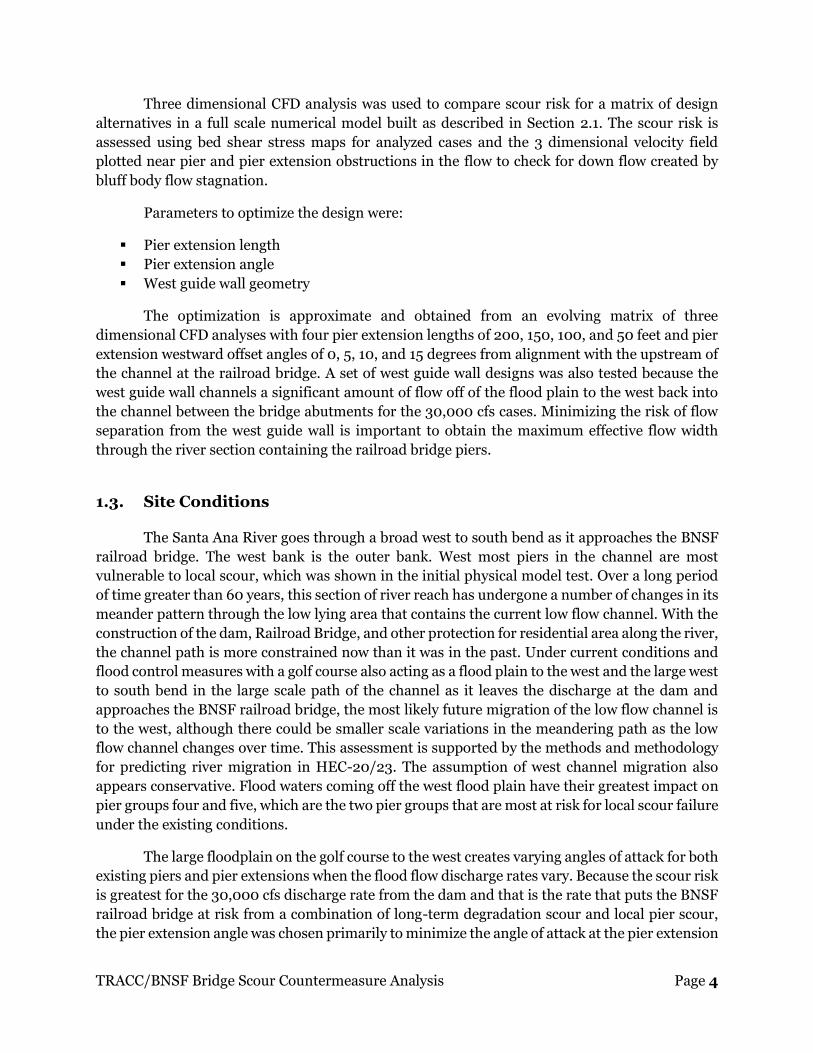
Three dimensional CFD analysis was used to compare scour risk for a matrix of design
alternatives in a full scale numerical model built as described in Section 2.1. The scour risk is
assessed using bed shear stress maps for analyzed cases and the 3 dimensional velocity field
plotted near pier and pier extension obstructions in the flow to check for down flow created by
bluff body flow stagnation.
Parameters to optimize the design were:
Pier extension length
Pier extension angle
West guide wall geometry
The optimization is approximate and obtained from an evolving matrix of three
dimensional CFD analyses with four pier extension lengths of 200, 150, 100, and 50 feet and pier
extension westward offset angles of 0, 5, 10, and 15 degrees from alignment with the upstream of
the channel at the railroad bridge. A set of west guide wall designs was also tested because the
west guide wall channels a significant amount of flow off of the flood plain to the west back into
the channel between the bridge abutments for the 30,000 cfs cases. Minimizing the risk of flow
separation from the west guide wall is important to obtain the maximum effective flow width
through the river section containing the railroad bridge piers.
1.3. Site Conditions
The Santa Ana River goes through a broad west to south bend as it approaches the BNSF
railroad bridge. The west bank is the outer bank. West most piers in the channel are most
vulnerable to local scour, which was shown in the initial physical model test. Over a long period
of time greater than 60 years, this section of river reach has undergone a number of changes in its
meander pattern through the low lying area that contains the current low flow channel. With the
construction of the dam, Railroad Bridge, and other protection for residential area along the river,
the channel path is more constrained now than it was in the past. Under current conditions and
flood control measures with a golf course also acting as a flood plain to the west and the large west
to south bend in the large scale path of the channel as it leaves the discharge at the dam and
approaches the BNSF railroad bridge, the most likely future migration of the low flow channel is
to the west, although there could be smaller scale variations in the meandering path as the low
flow channel changes over time. This assessment is supported by the methods and methodology
for predicting river migration in HEC-20/23. The assumption of west channel migration also
appears conservative. Flood waters coming off the west flood plain have their greatest impact on
pier groups four and five, which are the two pier groups that are most at risk for local scour failure
under the existing conditions.
The large floodplain on the golf course to the west creates varying angles of attack for both
existing piers and pier extensions when the flood flow discharge rates vary. Because the scour risk
is greatest for the 30,000 cfs discharge rate from the dam and that is the rate that puts the BNSF
railroad bridge at risk from a combination of long-term degradation scour and local pier scour,
the pier extension angle was chosen primarily to minimize the angle of attack at the pier extension

TRACC/BNSF Bridge Scour Countermeasure Analysis Page 5
nose for the highest discharge rate. A lower discharge rate of 10,000 cfs was also checked for any
dramatic change in scour risk for several angles of attack at the lower rate.
The topology of the area of the river reach is not flat and has significant variations in
elevations that impact the three dimensional flow patterns during floods. These variations
produce some relatively high shear areas due to local rising elevation during flood flows, these
areas are in general far enough away from the railroad bridge piers that they do not have a direct
impact on local scour risk at the piers, but the topology variations do have an indirect influence
on the overall channel flow that can affect the velocity distribution and bed shear in the region of
the piers. Topological variation in elevations on the golf course flood plain are significant because
there are natural lower elevation paths leading from the flood plain toward the main river channel.
Taking these into account in the design of the west guide wall was important.
1.4. Flow Physics Basis for Triangular Pier Extensions As Scour
Countermeasures
Piers, especially the semi rectangular BNSF bridge piers, are bluff body obstructions in the
river flow domain. As such, oncoming flow approaching the upstream pier bluff body surface will
have a stagnation point on the face. As the flow approaches the stagnation point, it spreads out in
all directions, much of it downward toward the riverbed. A riverbed composed of sediments can
be characterized as a porous wall with material properties that can be reduced to an effective
roughness, a porosity, and a permeability. Modeling the effects of these properties was not
included in the scope of this study. They are noted here because significant downflow toward the
bed caused by a bluff body pier obstruction increases the pore pressure in the sediment at the base
of the pier weakens the sediment and can contribution to scour. Characterizing soil strength can
involve many more soil property parameters and is also beyond the scope of this study. Water
upflow from a stagnation point will increase water depth locally on the upstream face of the pier,
which is more pronounced in higher velocity flood flows, and greater water depth also can
contribute to higher local pore pressure at the upstream base of the pier. While modeling these
effects was beyond the scope of this study, eliminating their contribution to local scour risk at the
base of piers with wedge shaped pier extensions that do not stagnate the flow or create any
significant down flow was a goal of the study.
The triangular shape of the pier extensions acts to streamline water flow around the piers
removing stagnation from the upstream surface. This kind of streamlining of body surfaces is
routinely applied in vehicle design to greatly reduce pressure drag on the vehicle body. The
triangular shape of the pier extensions yield minimal frontal area for flow stagnation at the
upstream nose as long as the angle of attack is small. If the angle of attack is large enough, flow
can stagnate on the sides of the pier extensions.
With increasing angle of attack, the risk of significant flow separation that may not
reattach for the length of the pier extension also increases. The separation zone contains eddies
with rotation that can be in a variety of orientations that may not align with the main flow. The k-
epsilon turbulence model used in this study does not capture these eddies, but does capture flow
separation from objects in the flow and approximate size and shape of the turbulent zone between

TRACC/BNSF Bridge Scour Countermeasure Analysis Page 6
a body or wall and the main flow. When the flow separates from a bank boundary wall or body
less effective area remains at that section to pass the flow and it will tend to accelerate, which
increases shear stress and scour of the bed. This reduction of overall flow area with consequent
increased scour is normally referred to as contraction scour.
Separation at a pier extension nose can result in local scour at the position of the nose on
the side where the separation occurs. This local scour risk is displaced upstream of the piers by
the length of the pier extensions. Part of the study is to check that any high shear patches caused
by separation from the nose of a bridge pier extension do not extend back to within a near vicinity
of the piers. Pier extension length needs to be sufficient to displace local scour risk at the nose
sufficiently far upstream.
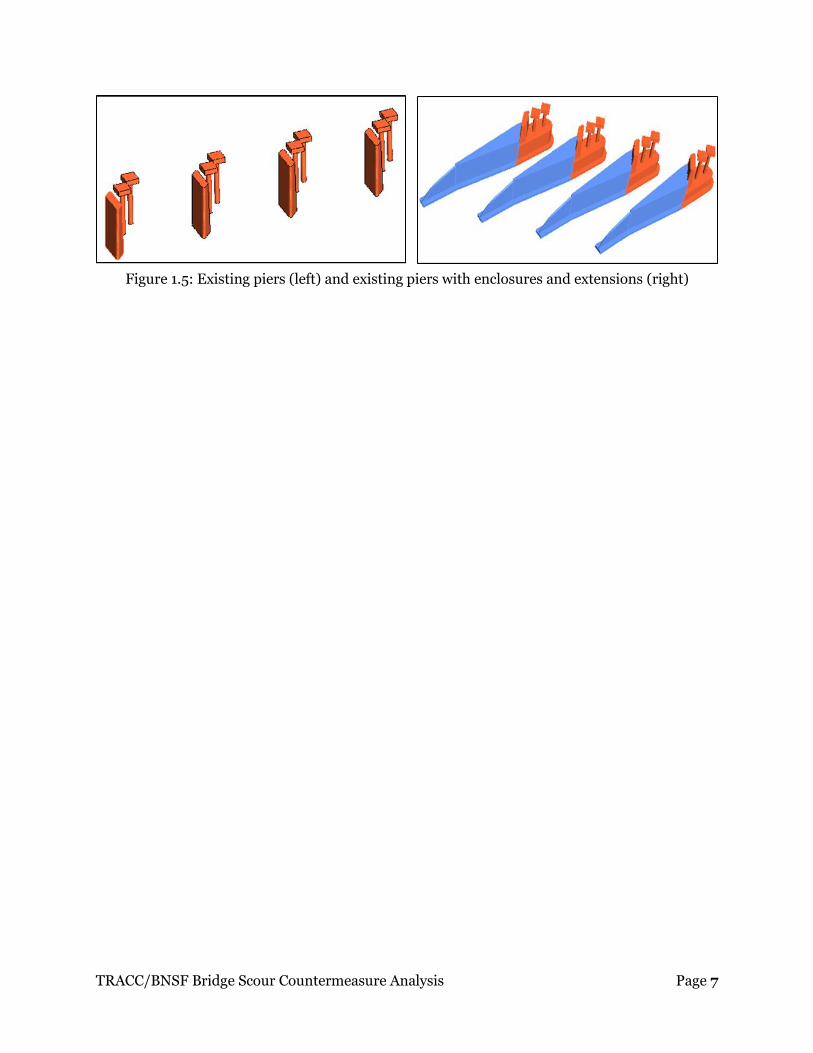
As shown in Figure 1.4, the originally proposed bridge pier extensions are triangular
wedges with a flat top. A 3 dimensional view of the piers with and without the proposed
countermeasures is shown in Figure 1.5. The pier extension nose is vertically tapered down from
the top of the extension wedge into the riverbed. This tapering has two beneficial effects. It diverts
upward the small portion of flow that approaches the nose directly from the front, and flow
separation from the nose due to angle of attack is spread along the length of the nose. Only a small
portion separates near the tip because the nose height tapers into the bed at the tip.
A vertically tapered nose spreads risk of flow separation due to angle of attack along the
length of the nose. At the tip only flow near the bed may separate. The vertically tapered nose also
causes any small amount of frontal flow at the nose tip to move upward.
Figure 1.4: Originally proposed bridge pier extension configuration – top and side views
TRACC/BNSF Bridge Scour Countermeasure Analysis Page 7
Figure 1.5: Existing piers (left) and existing piers with enclosures and extensions (right)

TRACC/BNSF Bridge Scour Countermeasure Analysis Page 8
2. Computational Model Geometries, Physics, and Case Set
The computational model consists of a set of full scale three dimensional geometries for
the test cases that comprise the computational domain for each case, and the two phase air-water
flow physics with free surface that is solved in the computational domain.
The geometry variations consist of the topology variations and variation of the geometry
of the pier extension and guide wall design. The topology variations focus on the current topology
of the channel and surroundings that may carry flow during flood flow conditions, and alternate
topologies that include variations of the channel path and long term degradation scour to test the
counter measure designs for robustness.
In this study four different topologies were analyzed:
1. Current topology and channel bathymetry: based on field surveys and satellite data
provided by USACE
2. Wide channel scoured bathymetry: in this case long term degradation was assumed to
scour most of the width across all pier groups down to 392 foot elevation due to channel
meandering over a long period of time
3. Narrow channel with long term degradation scour bathymetry and 100 foot west channel
migration
4. 300 foot west migrated channel with no long term degradation scour
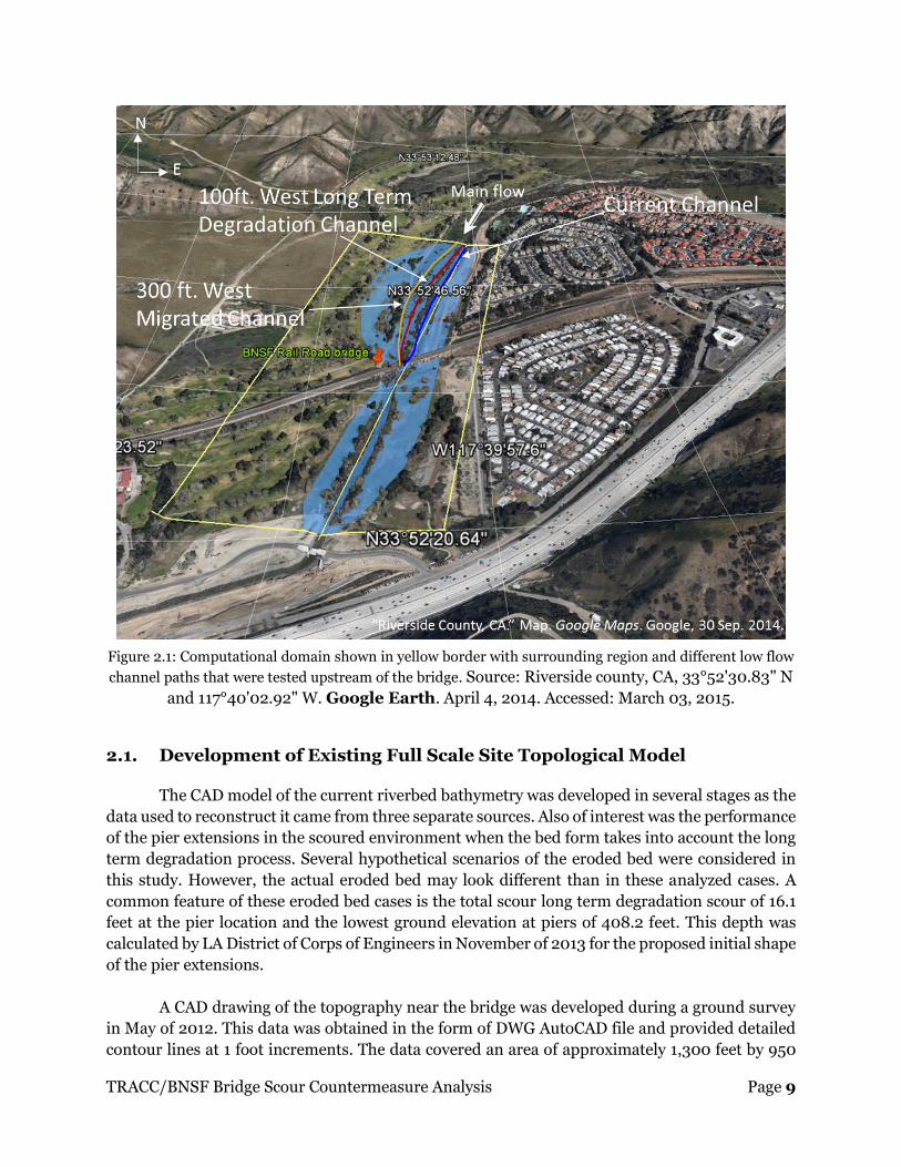
Figure 2.1 shows the computational domain outlined in yellow with portion of the
surrounding region including the housing developments to the east and golf course to the west.
The figure also shows the three courses of the channel that were tested. The path of the current
low flow channel is shown in blue, the path of the narrow channel with long term degradation
scour and 100 foot west migration is shown in red, and the path of the 300 foot west migrated
channel with no degradation scour is shown in yellow. The two west migrated channels must curve
back eastward to flow under the BNSF bridge. These topologies were created in part to test the
effects of varying angle of attack that might occur over time at the bridge.
TRACC/BNSF Bridge Scour Countermeasure Analysis Page 9
Figure 2.1: Computational domain shown in yellow border with surrounding region and different low flow
channel paths that were tested upstream of the bridge. Source: Riverside county, CA, 33°52'30.83" N
and 117°40'02.92" W. Google Earth. April 4, 2014. Accessed: March 03, 2015.
2.1. Development of Existing Full Scale Site Topological Model
The CAD model of the current riverbed bathymetry was developed in several stages as the
data used to reconstruct it came from three separate sources. Also of interest was the performance
of the pier extensions in the scoured environment when the bed form takes into account the long
term degradation process. Several hypothetical scenarios of the eroded bed were considered in
this study. However, the actual eroded bed may look different than in these analyzed cases. A
common feature of these eroded bed cases is the total scour long term degradation scour of 16.1
feet at the pier location and the lowest ground elevation at piers of 408.2 feet. This depth was
calculated by LA District of Corps of Engineers in November of 2013 for the proposed initial shape
of the pier extensions.
A CAD drawing of the topography near the bridge was developed during a ground survey
in May of 2012. This data was obtained in the form of DWG AutoCAD file and provided detailed
contour lines at 1 foot increments. The data covered an area of approximately 1,300 feet by 950

TRACC/BNSF Bridge Scour Countermeasure Analysis Page 10
feet. Figure 2.2 shows a screenshot of that data together with the location of the bridge and piers.
Using LS-PREPOST a free pre and post processor for finite element modeling (FEM) [3] this data
was broken down into a point cloud (see Figure 2.3).
Figure 2.2: CAD representation of the elevation contour lines
Figure 2.3: Point cloud representation of the vicinity of the bridge. Red color represents higher
elevation and blue represents lower elevations
Flow

TRACC/BNSF Bridge Scour Countermeasure Analysis Page 11
The upstream and the downstream topology was provided in a point cloud format (x, y, z
coordinates). Thus, the transformation of that data wasn’t necessary before merging it with the
rest of the data. The resolution of the upstream data was coarser than the resolution of the portion
in the bridge vicinity. However, it was sufficient for reconstruction of the bed for the CFD analysis
purposes. The data covered a much larger area than needed in this project. Figure 2.4 and Figure
2.5 show the point cloud data for the upstream and downstream respectively.
Figure 2.4: Point cloud representation of the ground upstream from the bridge. Red color
represents higher elevation and blue represents lower elevations
Figure 2.5: Point cloud representation of the ground downstream from the bridge. Red color
represents higher elevation and blue represents lower elevations
The point cloud data from these three areas was imported into MeshLab software [4] that
is able to transform subsets of point data and fit a triangularized surface into it. The data on the
boundaries of the three regions didn’t match perfectly. MeshLab is able to patch mismatched data
points with an averaged fit of a surface. A smoothed fit to the entire set of data was used as a basis
Flow

TRACC/BNSF Bridge Scour Countermeasure Analysis Page 12
for CFD models. A close up view on the triangulated point cloud data used in CFD analysis is
shown in Figure 2.6.
Figure 2.6: Fitting of a surface to mismatching data points in MeshLab software
Figure 2.1 shows an aerial view of the area with the CFD domain bordered in yellow lines.
The size of the CFD domain was selected in the process of expanding an initial model until the
assumed boundary conditions on the CFD domain were not influencing the results underneath
the bridge. Figure 2.7 shows the fitted surface to the merged point cloud data covering the CFD
analytical domain.
Figure 2.7: Current topology with elevation contours
Flow

TRACC/BNSF Bridge Scour Countermeasure Analysis Page 13
2.2. Alternative Topology Models for Long Term Degradation and Channel
Migration
The CFD analysis with the current bathymetry only provides information about the
performance of the pier extensions in the short term future. The ultimate performance of these
additions needs to be tested considering the long term degradation conditions in the river bed.
However, the shape of the eroded river channel is unknown. Two channels with long term
degradation scour topologies were constructed. One additional topology with the existing channel
depth but with a 300 feet migration westward into the golf course was also constructed to test
performance of the pier extensions with a large change in the approach flow angle of attack at the
pier extensions.
Constructing plausible channels with long term degradation scour was not an easy task.
The method used was to create a channel cross section at the bridge piers running out to and
merged into the channel banks just above the high water elevation for the 30,000 cfs flood as
shown in Figure 2.8 and Figure 2.10. These cross sections were then swept up and down stream
along the existing channel at the projected long term degradation scour elevations in LS-
PREPOST, LS-DYNA’s Pre and Post processing software [3]. Except for the bridge area, where the
channel cross section was created, the channel edges did not transition smoothly into the
surrounding topology. As a consequence, the local 3D terrain along the swept channel had to be
modified manually in CAD software along both sides of the channel to smoothly merge the new
channel edges with the varying local topology. This process was labor intensive and limited the
number of alternate topologies that could be constructed to the three presented in this section.
The first long term degradation scoured topology was a wide channel with uniform long
term degradation scour as shown in Figure 2.8. The flow cross-section is shown on the top of the
original bed form with the transparent blue area. It originates from the idea that a meandering
river could produce a wide channel eroded down to the depth of the long term degradation scour
over a long period of time. When this profile is swept up and downstream from the bridge, and
stitched back with the surrounding topology, it could possibly yield the topology shown in Figure
2.9.
Figure 2.8: Wide channel degradation scour channel flow cross-section shown in transparent
blue with maximum depth at 392 feet elevation
408 ft.
West Abutment East Abutment
Pier-5
Pier-6 Pier-4 Pier-3 Pier-2 Pier-1

TRACC/BNSF Bridge Scour Countermeasure Analysis Page 14
Figure 2.9: Wide degradation scour topology with elevation contours
The wide channel scour topology in the shape presented in Figure 2.9 is not very likely to
occur in reality. Even if it was formed in such shape it would be actually a desirable state. A wide
channel with increased cross section area can carry more volume of water at a lower speed,
decreasing the shear stress in the river bed and the risk of scour around the piers. For this reason
another bed shape was built with the maximum depth at the 392 foot elevation only close to pier
sets 4 and 5 and tapering slowly to the east and with a steep slope on the west side as presented
in Figure 2.10. That cross section with a relatively narrow low flow channel was extruded
upstream with a 100 foot west migration into the flood plain and almost straight south path in the
downstream direction. This long term degradation channel is only one of many that are possible,
however, it appears to be a more realistic estimate and a more conservative one for assessing
future scour risk than the one wide nearly flat channel topology.
Figure 2.10: New flow cross-section shown in transparent blue zone
Low flow channel
Pier-1 Pier-2 Pier-3 Pier-4 Pier-5
Pier-6
408 ft.
West Abutment East Abutment
Flow

TRACC/BNSF Bridge Scour Countermeasure Analysis Page 15
Figure 2.11: View of narrow long term degradation scoured channel
Figure 2.12: 300 foot west migrated channel with no degradation scour
Flow
Flow

TRACC/BNSF Bridge Scour Countermeasure Analysis Page 16
A comparison of elevations along the low flow channel for the current existing bathymetry
and the projections for the long term degradation scoured bathymetry is shown in Figure 2.13.
The long term degradation scour elevations were obtained from [5], and these were single point
values at a stream reach position with no information about channel cross section profile at that
position. The two long term degradation scour topologies were constructed to match this data
along the river reach in the domain of the model.
Figure 2.13: Current conditions profile and projected maximum general degradation over the
long−term flood series near the piers from [5]
The last artificial topology profile with a west channel migration of 300 feet was used to
study the effect of a maximum possible change of angle of attack of water on the pier extensions
and the consequent change in the bed shear stress patterns around the piers. The migrated
channel was curved back to the fixed point of the protected west bridge abutment and pier group
6, allowing for the water flow between pier groups 4 and 5. No degradation scour was included for
this case and the original cross section from under the bridge was swept along the artificial west
migrated channel line. The long term degradation scour profile had been shown to reduce bed
shear stresses and was not included to be conservative in testing effects of changing angle of attack
of flow and shear patterns at the bridge.
These 300 foot west migrated channel was intended to create a maximum condition for
flow from west to east in the approach to the bridge. The current topology is shown in Figure 2.7,
and the 300 foot west migrated channel topology is shown in Figure 2.12.
375
380
385
390
395
400
405
410
415
420
32,000 33,000 34,000 35,000 36,000 37,000
Ele
va
tio
n (
ft)
Distance (ft)
Current Bathymetry Scoured Bathymetry

TRACC/BNSF Bridge Scour Countermeasure Analysis Page 17
2.3. Tested West Guide Wall Design Geometries
The initial analysis revealed large separation developing off of the north corner of the west
guide wall. For that reason several alternative shapes of that wall were proposed in addition to
the pier extensions. The following designs were analyzed:
Original proposed guide wall
HEC-20/23 based guide wall
Topology conforming guide wall
The evolution of the west guide wall design is described in Section 3.5.3.
Figure 2.14: West guide wall configurations (a) original proposed guide wall, (b) HEC-20/23
based guide wall, and (c) topology conforming guide wall
2.4. Computational Model Physics
In this study, a simulation model was developed using the commercial CFD software
STAR-CCM+ version 9.06. Commercial CFD software was used because it is widely used in
industry for engineering design, each version is benchmarked against a large validation problem
TRACC/BNSF Bridge Scour Countermeasure Analysis Page 18
set, and it can therefore be considered very reliable for general engineering use. For most
turbulent flows of practical interest, a turbulence model is required to allow a solution of the flow
field to be computed, even on large clusters, with a reasonable use of resources and time. STAR-
CCM+ software has a wide range of turbulence models available, including a variety of commonly
used one equation and two equation models, a Reynolds stress model, and both large eddy
simulation (LES) and detached eddy simulation (DES) models. LES and DES, while providing the
most detailed characterization of a flow field are too expensive and time consuming for this
applied study involving a large number of cases. The STAR-CCM+ 3D CFD model used here solves
the Unsteady Reynolds Averaged Navier-Stokes (URANS) equations that govern fluid flow. These
are the conservation of mass and Newton’s 2nd law applied to a control volume through which the
fluid flows. The governing equations are listed in Section 2.4.3. The URANS equations are derived
by splitting the flow variables into a mean and fluctuating component and then averaging the
governing equations on a time scale that is long with respect to the scale of small fluctuations. In
the averaging process, the variables for the fluctuating components associated with turbulence
end up in cross correlations of fluctuating velocities, commonly referred to as Reynolds stresses,
that remain in the URANS equations and are new unknown variables. A turbulence model
replaces these cross correlations with expressions in terms of the turbulence model variables,
usually including an eddy viscosity, 𝜇𝑡, that accounts for the greatly increased transport of fluid
properties due to turbulence.
The k-epsilon turbulence model was chosen for this work because it is one of the most
robust and widely used in industry and it works well for free surface flows. The k-epsilon model
adds two transport equations with model variables for the turbulent kinetic energy, k, and its
dissipation rate, epsilon, ε. In this model the eddy viscosity is given by
𝜇𝑡 = 𝐶𝜇𝜌𝑘2/𝜖
where 𝐶𝜇 was originally a model constant [15], 0.09, but in the more advanced k-epsilon model
used here is a constant plus a function of mean flow and turbulence model variables [7].
The discretization of the governing equations is done for this software using the control
volume method. The domain is divided into small volumes, the computational cells, and the
discrete equations are obtained by integrating the governing equations over the computational
cells with appropriate assumptions, for example a fluid property such as velocity is assumed to be
constant over a small control volume cell face. To make the derivation of discrete equations
straightforward in the control volume method (CVM), the governing equations are left in integral
form, as they are in the list in Section 2.4.3. The set of cells or cell centroids is referred to as the
computational grid or mesh. Computational cells in STAR-CCM+ can be composed of tetrahedral,
hexahedral, or polyhedral cells. Tetrahedral cells are a legacy cell type that are not used because
they create relatively high numerical diffusion. Hexahedral cells are well suited when the flow is
primarily in one direction, and polyhedral cells are good for flows that are turning through the
domain. Polyhedral cells have 12 to 14 faces. A polyhedral mesh was used to accurately capture
the flow over the varying topology of the channel and flood plains in the domain and it allows
continuous and smooth variation of cell volume, which was constructed to be finer near the
features of interest including the piers and extensions and the varying bed topology.

TRACC/BNSF Bridge Scour Countermeasure Analysis Page 19
Resolving the boundary layer at the bed with enough computational cells to get a velocity
profile sufficiently accurate to compute bed shear from the definition as viscosity times the
velocity gradient normal to the wall would be far too expensive for this type of parametric design
study. Therefore, the viscus sublayer is not resolved in the computational grid, and the shear
stress at the bed is computed from turbulence model variables and velocity at the near wall cell
centroid using the two-layer, all y-plus wall functions. The value of y-plus is a non-dimensional
distance from the wall or bed, 𝑦+ = 𝑦𝑢𝜏/𝜈, where 𝑢𝜏 is the shear velocity and ν is the kinematic
viscosity of the fluid. For y-plus greater than 30, the velocity profile is assumed to be determined
by the logarithmic law of the wall, for y-plus less than about 30, various blended formulations are
used to obtain a bed shear stress that is accurate enough for engineering applications [7].
The flood flows modeled in this study are water flows with a free surface with air above
and water below that may vary in height as a consequence of both local and upstream and
downstream conditions. The volume of fluid (VOF) model captures the free surface profile
through use of a variable representing the volume fraction of the water in a computational cell.
An additional transport equation listed in Section 2.4.3 is solved to obtain the volume fraction of
water in computational cells that contain the free surface, and therefore a mixture of air and water.
The air fraction is one minus the water volume fraction. This multiphase physics model is referred
to as the VOF model for free surface flow simulations and was used to model the air-water flow
for the flood simulations in this study. In the VOF model, the fluids, in this case air and water are
considered immiscible and additional equations and algorithms are used to maintain the
separation of the fluids and integrity of the free surface. The details of these are not provided here,
and the interested reader is referred to the STAR-CCM+ user guide [7].
The CFD model uses the full scale detailed topology 1900 feet upstream, 1500 feet
downstream of the bridge, and 1500 feet across the channel including the flood plain to the west
as shown previously in Figure 2.1. The computational flow domain is located about 10,000 feet
downstream of the Prado dam outlet channel. It is the region bordered by yellow in Figure 2.1.
The current bed elevation of the channel and surroundings are shown in Figure 2.7.
In Figure 2.10, a cross-section view of the bed topology is shown, where the current
bathymetry bed profile is shown as an edge of brown shaded area, while the long term degradation
scour bathymetry bed profile is shown as a transparent blue shaded area. The existing bathymetry
consists of a low flow channel with the deepest point at 408 feet of elevation at the bridge. For the
case of long term degradation scour, the maximum depth of the channel at the bridge is at an
elevation of 392 feet. Further, long term degradation scour bathymetry also includes a stream
meander and migration approximation based on the methods of NCHRP-533 report [5]. This
report suggests stream migration in the westward direction into the flood plain. Data was not
readily available to use NCHRP 533 techniques to predict the extent of future migration based on
past trends, and a best estimation of the migration was made using the principles in NCHRP-533
in combination with constraints in the site topology. Hence, the long term degradation scour river
channel bathymetry was moved 100 foot westward to test the effect of this migration. The
computational domain contains guide walls at the east bank between pier groups 1 and 2 and at
the west bank between pier groups 5 and 6. The west bank guide wall went through several design
variations. The first west guide wall redesign used guidelines provided in HEC-20/23 [6, 7] to
guide the flood plain water into the main channel with minimum separation probability. That
TRACC/BNSF Bridge Scour Countermeasure Analysis Page 20
methodology works well for a relatively flat terrain, but did not work well for the existing
topological variations on the flood plain at the site. Consequently, the west guide wall underwent
a second redesign as detailed in Sections 2.3 and 3.4.
2.4.1. Assumptions
Using the unsteady Reynolds Averaged Navier Stokes equations with a k-epsilon
turbulence model was assumed to be sufficient for the comparative scour risk assessments
needed in this study.
Eddies, periodically shed from structures, passing over the bed cause fluctuations in the
bed shear stress as they pass by. When bed shear is below that needed for onset of sediment
entrainment, the passage of an eddy can raise it above that threshold. Large eddy simulation (LES)
or detached eddy simulation (DES) can identify areas where fluctuating bed shear stress oscillates
above and below that needed for onset of sediment entrainment. Those areas may be missed using
a k-epsilon model when the mean bed shear is near but below critical over most of the bed. In the
cases analyzed in this study, however, the bed shear under flood conditions is well above critical
for nearly all of the bed particle range size at the site. Therefore, any underestimation of
entrainment rates would be at most a small secondary effect. In addition, bed shear maps are used
primarily for comparison between alternative geometry and bed topology conditions to assess
relative scour risk and no scour entrainment rate is calculated from the mean bed shear values.
The cost of running either LES or DES simulations would be prohibitively expensive and the time
needed to complete all the cases that were analyzed would far exceed the time available to
complete the study. Therefore use of the k-epsilon turbulence is good enough to obtain the
engineering data needed to achieve the goals of the study within the time and budget of the
project.
The effects of vegetation within the domain are not modeled.
The site contains trees, bushes, and grass that are not part of the model. Additional flow
resistance could have been included in the analysis by adding tree trunks and meshing them,
including bushes as small volumes of porous media, and grass in a variety of ways. These additions
would have been very time consuming to incorporate and would have added additional complexity
to the model physics that would have also increased the required work by an amount that would
not have been acceptable within the time constraints of the project. Exclusion of the modeling of
vegetation is not expected to have a major impact on results and should be good for engineering
assessment. A major effect of vegetation is to hold soil in place, especially grass on the golf course,
but this does not affect the model because an actual 3D scour simulation is beyond the capabilities
of current commercial software, rather scour risk is assessed based on bed shear stress and
stagnation with downflow on bluff bodies like piers in the flow. Knowing that grass would offer
more resistance to scour than loose bed material, any high shear zones in areas with grass are
simply less at risk for significant scour, and are of less interest because they are not near the bridge
piers.
The bed is assumed to be smooth.

TRACC/BNSF Bridge Scour Countermeasure Analysis Page 21
The actual bed material is primarily fine grained with variation that includes larger
pebbles and rocks. Because relative bed shear between the different cases for topology and pier
extension and guide wall design is compared to assess relative scour risk, bed shear results that
are shifted by the same amount do not affect the conclusions and are good enough for engineering
accuracy.
2.4.2. Uncertainties
The accuracy of the bed topology for existing conditions is limited to that of the provided
point cloud and survey used to build the domain. The points in the point cloud topology data were
varying between one and several feet of separation. The AutoCAD data for elevation contour lines
in the vicinity of the bridge were spaced about one foot apart.
The free surface water level in the river is resolved to about ±1/2 foot due to grid cell size
and density smearing at many locations where the free surface does not align with the grid. The
VOF model averages material properties in computational cells that contain the free surface
weighted by the fraction of the cell occupied by water and air respectively. Advection of this
averaged mixture into the downstream can produce density smearing where the free surface
appears to be smeared out over several vertical cells. Although the sharp location of the free
surface is not preserved, the mass of water is conserved to several significant digits. The location
of the free surface is taken to be the height where the volume fraction of water is equal to 0.5. This
is the exact location of the free surface when that surface is finely resolved and it is the best
engineering estimate of the location when some density smearing at the air water interface has
occurred.
The boundary layer along the bed is not resolved in the grid. Doing so would make the
model far too large and expensive to run. Instead a variation of standard wall functions is used to
compute the shear stress at the bed, see Section 2.4.3. Uncertainty in this model can be around
ten percent, and is close to as good as other more sophisticated and computationally intensive
techniques. It is sufficiently good for most engineering applications.
2.4.3. Governing Equations
The models were run using the full three dimensional geometry of the domain. For the
problem at hand, the Realizable Two-Layer k-ε turbulence model was used with all-y+ wall
treatment since this model works well when there are varying mesh densities in the domain and
the distance of a cell centroid in the cell next to the wall may not always lie in the range where the
logarithmic law of the wall applies [7, 12, 13].
The Segregated Fluid Isothermal model and associated solvers were used in the
simulation. The governing unsteady form of the unsteady Reynolds Averaged Navier Stokes
(URANS) equations in the STAR-CCM+ User Guide [7] are given in integral form as follows.
Conservation of mass:
𝜕
𝜕𝑡∫ 𝜌 𝑑𝑉
𝑉
+ ∮ 𝜌(𝑣 − 𝑣𝑔) ∙ 𝑑𝒂
𝐴
= 0

TRACC/BNSF Bridge Scour Countermeasure Analysis Page 22
Conservation of momentum, Newton’s 2nd law for fluid motion:
𝜕
𝜕𝑡∫ 𝜌𝒗 𝑑𝑉
𝑉
+ ∮ 𝜌𝒗 ⊗ (𝒗 − 𝒗𝒈) ∙ 𝑑𝒂
𝐴
= − ∮ 𝑝𝐈 ∙ 𝑑𝒂
𝐴
+ ∮ 𝜇𝑒𝑓𝑓 [∇𝒗 + ∇𝒗𝑻𝐈] ∙ 𝑑𝒂
𝐴
+ ∫ 𝑓𝑔 𝑑𝑉
𝑉
Transport equation for turbulent kinetic energy, k:
𝜕
𝜕𝑡∫ 𝜌𝑘 𝑑𝑉
𝑉
+ ∮ 𝜌𝑘(𝒗 − 𝒗𝒈) ∙ 𝑑𝒂
𝐴
= ∮ (𝜇 +𝜇𝑡
𝜎𝑘) ∙ 𝑑𝒂
𝐴
+ ∫[𝑓𝑐𝜇𝑡𝑆2 − 𝜌(𝜖 − 𝜖0)] 𝑑𝑉
𝑉
Transport equation for turbulent dissipation rate, ε:
𝜕
𝜕𝑡∫ 𝜌𝜖 𝑑𝑉
𝑉
+ ∮ 𝜌𝜖(𝒗 − 𝒗𝒈) ∙ 𝑑𝒂
𝐴
= ∮ (𝜇 +𝜇𝑡
𝜎𝜖) ∙ 𝑑𝒂
𝐴
+ ∫ [𝑓𝑐𝐶𝜖1𝜖𝑆2 −𝜖
𝑘 + √𝜈𝜖𝐶𝜖2𝜌(𝜖 − 𝜖0)] 𝑑𝑉
𝑉
where:
A control volume surface vg grid velocity = zero
𝒂 computational cell face area vector ⊗ tensor dyadic product
𝐶𝜖1 turbulence model coefficient [7] ∇ del operator
𝐶𝜖2 turbulence model constant = 1.9 𝜖 turbulent dissipation rate
fc curvature factor 𝜖0 dissipation limit for minimum low
level background turbulence
𝑓𝑔 body force due to gravity µ fluid dynamic viscosity
I identity matrix µt eddy or turbulent viscosity
p pressure µeff effective viscosity = µ + µτ
S modulus of strain rate tensor ν kinematic viscosity
V computational cell volume 𝜌 density
t time 𝜎𝑘 turbulence model constant = 1.0
v velocity vector 𝜎𝜖 turbulence model constant = 1.2
vT transpose of velocity vector

TRACC/BNSF Bridge Scour Countermeasure Analysis Page 23
In the VOF free surface model only one momentum equation is solved because the fluids
are always separated by the free surface. In mesh cells that contain the free surface, the material
properties of the fluid in those cells is determined by averaging as follows:
𝜌 = ∑ 𝜌𝑖𝛼𝑖
𝑖
𝜇 = ∑ 𝜇𝑖
𝑖
𝛼𝑖 𝑐𝑝 = ∑(𝑐𝑝)𝑖 𝜌𝑖
𝜌𝛼𝑖
𝑖
where αi = Vi/V is the volume fraction, Vi is the volume occupied by the i th phase, and 𝜌𝑖, 𝜇𝑖, and
(𝑐𝑝)𝑖 are the density, molecular viscosity, and specific heat of the i th phase respectively.
The conservation equation that describes the transport of volume fraction, 𝛼𝑖, is:
𝑑
𝑑𝑡∫ 𝛼𝑖𝑑𝑉
𝑉
+ ∫ 𝛼𝑖(𝑣 − 𝑣𝑔) ∙ 𝑑𝒂 = 0
𝐴
For only two phases, air and water, only one phase volume equation needs to be solved because
the volume fraction of the other phase is one minus that of the solved for volume fraction.
Additional details on the complete model governing equations, including the transport
equations for the turbulent kinetic energy and dissipation rate in the k-epsilon turbulence model
and the wall functions used to compute bed shear can be found in the STAR-CCM+ User Guide
[7].
2.4.4. Boundary Conditions, Solver Controls, and Convergence Criteria
The model consists of two types of bathymetry, current and long term degradation scour
bathymetry. In both cases an extended rectangular channel is used to prevent recirculation near
the outlet. At the inlet boundary, the velocity and water level is specified in such a way that the
volume flow rate at the inlet remains at the flood flow rate. As upstream conditions are unknown
in terms of velocity and water level, an iterative procedure is used to choose velocity at the inlet.
A pressure boundary condition is used at the outlet to mimic the back pressure that would
normally be present due to water immediately downstream in a continuing channel. Further, in
the cases with scoured bathymetry where the river bed is lowered by ~16 feet in the west half of
the channel, a weir was used at the outlet boundary to avoid a super critical flow transition
downstream of the bridge and maintain a sufficient water level in the channel in that region. The
river bed is currently assumed to be a smooth surface. For some cases an inlet and outlet reservoir
had to be constructed to achieve a stable solution with reasonable water depths in the domain,
usually a water depth of about 22 feet at the bridge.
TRACC/BNSF Bridge Scour Countermeasure Analysis Page 24
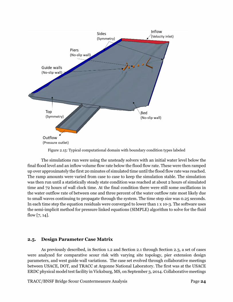
Figure 2.15: Typical computational domain with boundary condition types labeled
The simulations run were using the unsteady solvers with an initial water level below the
final flood level and an inflow volume flow rate below the flood flow rate. These were then ramped
up over approximately the first 20 minutes of simulated time until the flood flow rate was reached.
The ramp amounts were varied from case to case to keep the simulation stable. The simulation
was then run until a statistically steady state condition was reached at about 2 hours of simulated
time and 72 hours of wall clock time. At the final condition there were still some oscillations in
the water outflow rate of between one and three percent of the water outflow rate most likely due
to small waves continuing to propagate through the system. The time step size was 0.25 seconds.
In each time step the equation residuals were converged to lower than 1 x 10⁻³. The software uses
the semi-implicit method for pressure linked equations (SIMPLE) algorithm to solve for the fluid
flow [7, 14].
2.5. Design Parameter Case Matrix
As previously described, in Section 1.2 and Section 2.1 through Section 2.3, a set of cases
were analyzed for comparative scour risk with varying site topology, pier extension design
parameters, and west guide wall variations. The case set evolved through collaborative meetings
between USACE, DOT, and TRACC at Argonne National Laboratory. The first was at the USACE
ERDC physical model test facility in Vicksburg, MS, on September 3, 2014. Collaborative meetings

TRACC/BNSF Bridge Scour Countermeasure Analysis Page 25
continued via additional web conference meetings through the fall and early winter as analysis
results were accumulated. These collaborative meetings allowed all project team members to
assess current modeling results and make decisions on what alternatives to try next to make most
efficient use of the computational resources and effort in running simulations. The cases are listed
in Table 1.
Running a full 3D simulation for the cases in Table 1, even with the computationally
efficient k-epsilon turbulence model using URANS equations still requires the resources of a high
performance computer cluster. The computational mesh is finer in the vicinity of features of
interest such as the piers and pier extensions and varied from about 2.5 million cells to 5 million
cells. Running a case to a quasi-steady state with mass balance between inlet and outlet for the
water required about 72 hours on 128 cores, or 8 nodes on the TRACC Zephyr cluster. Each Zephyr
compute node has two processors with 8 floating point cores per processor. The nodes are
connected with a 40 gigabit per second Inifniband interconnect. Run times did vary with case,
and often inlet water level had to be adjusted during running a case to satisfy downstream flow
conditions. While a large number of cases could be run in comparison to the number of physical
model cases that could be run in the same time period, about 8 months, completing the cases in
the case table was still a major undertaking. Consultation with the project engineers at USACE in
California, and the physical modeling engineers at the USACE ERDC laboratory was very valuable
in keeping the number of cases in the case table at a level that could be completed in the required
time.
Due to limited computer resources and time, not all combinations of design parameters
could be tested. The case table lists most of the cases that were run with some additional sets of
cases listed in the text below the table.
Most of the cases run used the existing topology, 31 of the 52 cases listed in the table. The
existing topology was the most trusted topology for testing with CFD analysis because it is a known
topology at the site that was formed by a combination of natural forces and human projects over
a long period of time. The other 3 topologies used for testing performance of the design in varying
conditions were plausible estimates based on model projections and rough estimates from the
Federal Highway Administration (FHWA) guidelines.
Pier extensions varying in length from the original proposed design of about 200 feet down
to 25% of that design length, about 50 feet, were tested with various combinations of the other
parameters but far from all of them. Once about 50% of the original length, 100 feet, was identified
as the a good length to balance the goals of displacing local pier scour risk sufficiently far upstream
and minimizing sensitivity to angle of attack, a large fraction of cases run after that were with the
100 foot extensions.
The extension angle parameter is the angle of the extension with respect to the original
proposed design, which was nearly aligned with the low flow channel in the immediate upstream
of the bridge but slightly east of the approach flow of the 30,000 cfs flood with water coming off
of the west flood plain. Extension angles of 0, 5, 10, and 15 degrees were tested, but most cases
were either the original design or a 10 degree westward shift for reasons explained in Section 3.3.

TRACC/BNSF Bridge Scour Countermeasure Analysis Page 26
The west guide wall underwent two redesigns described in detail in Section 3.4. The most
important CFD cases were repeated for the two west guide wall redesigns to verify that
conclusions or decisions made from previous tests were still valid.
Table 1: Simulation Case Set
Cases Topology Extension
Length Extension
Angle West
Guide Wall Note
1 Existing No Extension N/A Original
proposed
2 Existing 100%
(~200ft) 0
Original proposed
3 Existing 100%
(~200ft) 5
Original proposed
4 Existing 100%
(~200ft) 10
Original proposed
5 Existing 80% (~160ft) 0 Original
proposed
6 Existing 50% (~100ft) 0 Original
proposed
7 Existing 100%
(~200ft) 0
Original proposed
Vertical Tapered Pier Extensions
8 Existing 100%
(~200ft) 10
Original proposed
Vertical Tapered Pier Extensions
9 Existing 100%
(~200ft) 0 HEC 20/23
10 Existing 100%
(~200ft) 10 HEC 20/23
11 Existing 50% (~100ft) 0 HEC 20/23
12 Existing 25% (~50ft) 0 HEC 20/23
13 Existing 50% (~100ft) 10 HEC 20/23
14 Existing 25% (~50ft) 10 HEC 20/23
15 Existing 50% (~100ft) 15 HEC 20/23
16 Wide
degradation 100%
(~200ft) 0
Original proposed
17 Wide
degradation 100%
(~200ft) 10
Original proposed
18 Wide
degradation 75% (~150ft) 0
Original proposed
19 Wide
degradation 50% (~100ft) 0
Original proposed
20 Wide
degradation 100%
(~200ft) 0
Original proposed
Vertical Tapered Pier Extensions
21 Narrow
degradation No Extension N/A
Original proposed

TRACC/BNSF Bridge Scour Countermeasure Analysis Page 27
Cases Topology Extension
Length Extension
Angle West
Guide Wall Note
22 Narrow
degradation 100%
(~200ft) 0
Original proposed
23 Narrow
degradation 100%
(~200ft) 10
Original proposed
24 Narrow
degradation 75% (~150ft) 10
Original proposed
25 Narrow
degradation 50% (~100ft) 0
Original proposed
26 Narrow
degradation 50% (~100ft) 10
Original proposed
27 Narrow
degradation No Extension N/A HEC 20/23
28 Narrow
degradation 100%
(~200ft) 0 HEC 20/23
29 Narrow
degradation 100%
(~200ft) 10 HEC 20/23
30 Narrow
degradation 50% (~100ft) 0 HEC 20/23
31 Narrow
degradation 50% (~100ft) 10 HEC 20/23
32 Narrow
degradation 100%
(~200ft) 10 HEC 20/23
Except Pier-5. angle set to
zero
33 Narrow
degradation 50% (~100ft) 10 HEC 20/23
Except Pier-5. angle set to
zero
34 Existing 50% (~100ft) 10 HEC 20/23 Extended guide wall
35 Existing No Extension N/A Topology conform
36 Existing 100%
(~200ft) 0
Topology conform
37 Existing 50% (~100ft) 0 Topology conform
38 Existing 25% (~50ft) 10 Topology conform
39 Existing 50% (~100ft) 10 Topology conform
40 Existing 75% (~150ft) 10 Topology conform
41 Existing 50% (~100ft) 15 Topology conform
42 Existing 100%
(~200ft) 10
Topology conform
Except Pier-5. angle set to
zero

TRACC/BNSF Bridge Scour Countermeasure Analysis Page 28
Cases Topology Extension
Length Extension
Angle West
Guide Wall Note
43 Existing 50% (~100ft) 10 Topology conform
Except Pier-5. angle set to
zero
44 Existing 100%
(~200ft) 0 HEC 20/23
10k cfs flow rate
45 Existing 100%
(~200ft) 10 HEC 20/23
10k cfs flow rate
46 Existing 50% (~100ft) 10 HEC 20/23 10k cfs flow
rate
47 Existing 50% (~100ft) 0 Topology conform
10k cfs flow rate
48 Existing 50% (~100ft) 10 Topology conform
10k cfs flow rate
49 Existing 25% (~50ft) 10 Topology conform
10k cfs flow rate
50 Narrow
degradation 50% (~100ft) 10
Topology conform
51 300ft Migrated 50% (~100ft) 10 Topology conform
10k cfs flow rate
52 300ft Migrated 50% (~100ft) 10 Topology conform
33k cfs flow rate
A number of additional simulations were performed as test cases. These include
1. At least 5 cases were run to adjust the water level in the domain based on the information
available on flood flow depths.
2. About 10 simulations were performed before finalizing the current site condition topology
3. Four additional simulations were performed for a near flat scoured bathymetry in the
vicinity of the piers
4. Four simulations were performed with variations of the topology conforming west guide
wall design

TRACC/BNSF Bridge Scour Countermeasure Analysis Page 29
3. Results and Discussion
3.1. Effect of Pier Extensions on the 3D Velocity Distribution at Piers and
Their Impact on Local Scour Risk
The flow structure commonly referred to as a horseshoe vortex forms around the front and
sides of a symmetric bluff body, like a cylinder, sitting in a uniform oncoming flow on a flat
surface. The churning action near the bed of large rotating turbulent flow structures like these are
a major cause of local scour near bluff body obstructions like piers. The semi-rectangular
upstream piers are not symmetric with respect to the approach flow and the approach flow is over
a non-flat varied topology, and therefore, a symmetric horseshoe vortex shedding eddies off the
sides of the structure would not be expected. However, similar non-symmetric unsteady vortex
structures forming at the piers of the BNSF bridge are expected and the wedge shaped pier
extensions on the upstream side were designed to prevent their formation.
Capturing the details of large eddy action and visualizing it requires the much more costly
and time consuming large eddy simulation, consuming weeks to a couple of months of run time
on a large parallel cluster for one case. In this study, the unsteady 3D Reynolds Averaged Navier
Stokes (URANS) equations are solved, which average out most of the rapidly changing eddy
structures. The K-epsilon turbulence model was employed to model the effects of the rapidly
evolving eddies including a large increase in bed shear caused by turbulent flow. Due to its ability
to yield rapid results of sufficient engineering accuracy, the 3D URANS model is widely used in
industry, except for cases where detailed resolution both in space and time, of rapidly evolving
eddy structures is clearly needed. Using URANS is sufficient to satisfy the engineering objectives
of this study.
The 3D flow fields for the cases in this study are complex due to the uneven topology and
asymmetric semi-rectangular piers with cylindrical piers in their wake. A wide variety of
visualization plots of the flow results from the URANS computations can be created from the 3D
flowfield, and several are included below that provide insight into scour risk for the cases without
pier extensions and near elimination of local scour risk due to bluff body obstruction on the
upstream side of the piers when the extensions are present.
Figure 3.1 through Figure 3.3 are all for a 30,000 cfs case, which corresponds to a 100 year
flood event. The velocity vectors show the direction of the flow without their magnitude. There is
a large discrepancy between the velocity magnitudes at different locations and vectors
proportional to the magnitude of velocity would be hardly noticeable at these spots, for example
in the wakes of the piers. Velocity direction vectors are plotted for the first layer of computational
cells near the bed and the pier wall surfaces, as well as on a vertical cut plane through the pier set
4, the second from the west guide wall. The cut plane is shaded gray to make it easier to visualize
the 3D position of the vectors. The position where the vectors stop on the cut plane is the water
free surface level along that plane. Velocity vectors near the pier surface also stop at the free
surface. These is air flow above, which also has a stagnation point on the pier but it is not shown
because it does not affect the water flow. Vectors with their tails on the cut plane are dark black

TRACC/BNSF Bridge Scour Countermeasure Analysis Page 30
when they have an out of plane component to the right and are a lighter color when they have an
out of plane component to the left (staying behind the cut surface).
Figure 3.1 below shows vectors near piers pointing every which way in the pier wakes, an
indication of how complex the flow pattern can be, even in a URANS computation, at an instant
in time. A pair of oval areas where there is flow stagnation on the 2 cylindrical piers or pier group
4 facing out of the picture is clearly visible however, and there is some down flow velocity there
but it is not strong enough in the lower velocity wake region to create high shear on the bed below
resulting in blue shading on the shear color scale.
Figure 3.1: Visualization of the velocity vectors near bed and wall surfaces and on vertical cut
plane through pier set 4, looking south for 30k cfs flood with current bed conditions shear stress
is color plotted on the bed
Figure 3.2 is a close up of this scene at pier group 5, the group just east of the west guide
wall. There is a noticeable stagnation point about half the way up near the rounded right corner
of the pier. There is a downflow below it that spreads left and right to go around the pier. At the
bed where there is the downflow near the pier face, there is some reverse flow toward the
upstream. That reverse flow stagnates at the low shear blue spot and turns left and right to make
its way around the pier. The flow accelerates as it moves around the pier in a reduced flow area.
Near the bed this results in the high shear zones off the edges represented by red color spots on
the bed. This pattern is close to what is expected from a horseshoe like vortex. However, a circular
vortex in the vertical cut plane sitting off the front of pier group 4 is not visible. That might be a
result of using a URANS model and the selected mesh resolution.
Flow

TRACC/BNSF Bridge Scour Countermeasure Analysis Page 31
Figure 3.2: Close up of near surface velocity vectors on pier set 5 (next to west guide wall)
showing stagnation on forward face, down flow, reverse flow, and turning flow around the front
of the semi-rectangular pier
The wedge shaped pier extensions with downward sloped tips were proposed by the U.S.
Army Corps of Engineers [9] as a countermeasure to avoid the flow stagnation that occurs on a
wide bluff body front face of the existing piers. For flow past the pier extensions, a horseshoe like
vortex structure would not be expected to appear near the tips. As shown in Figure 3.3 and Figure
3.4, the flow follows the upward sloping tip of the extension to the point where there is a short
vertical jump up to the top of the extension. There is flow stagnation at that height and velocity
vectors spreading out from it are visible. Note that if the flow is not aligned with the long axis of
an extension nose, there can be varying degrees of flow separation off the tip with accompanied
acceleration that can produce some high shear on the bed to one side of the tip. Such zones are
larger when the angle of attack increases, and will result in local scour off the extension nose.
However, the scour would be displaced upstream away from the existing bridge piers, which was
one of the goals of the mitigation design.
Figure 3.4 shows velocity direction vectors of flow just off the surface of pier extension 4,
the second from the west. The only flow stagnation points on the extension are at the step up from
the upward slope of the nose to the top of the wedge, which has been eliminated from the final
design recommendation. There are no vertical down flows caused by stagnation. Flow direction
on the sides is either upward or parallel to the bed. Flow parallel to the bed may be slightly
downward when the channel bed next to the extension is sloped downward.

TRACC/BNSF Bridge Scour Countermeasure Analysis Page 32
Figure 3.3: Velocity direction vectors on a gray shaded vertical cut plane aligned with the middle
of the pier extension wedge of pier group 4
Figure 3.4: Water velocity pattern on upstream side of pier with extension
3.2. Design of Extension Length
A range of pier extension lengths from the original proposed design of length 200 feet
down to one quarter of that, about 50 feet was tested in a variety of cases. The recommended
length of 50% of the original proposed design is based on a number of interrelated goals and flow
behavior with varying flood conditions. These are discussed in the following paragraphs. Shorter
extensions save construction costs, and therefore one goal is to reduce length to reduce cost.
The effect of the orientation of the pier extensions on the approach flow extends a long
distance into the upstream, and the pier extensions are sensitive to large angles of attack. The

TRACC/BNSF Bridge Scour Countermeasure Analysis Page 33
angle of attack changes with the amount of water flowing off of the west flood plain to join the
main flow approaching the narrower channel under the bridge. Shorter extensions allow more
distance for the flow to move eastward off the flood plain when merging with the main flow
reducing variation in angle of attack for different flood flow conditions. These interrelated effects
at this site mean that shorter extensions should function better under a variety of flood conditions.
The local shielding effect of the extensions at the piers is very effective in avoiding bluff
body flow stagnation, down flows, flow separation at the piers, and large acceleration in the
diverted flow as described in Section 3.1. These streamlining benefits for the bluff body piers are
relatively insensitive to pier extension length as long as flow does not separate due to a large angle
of attack of the approach flow.
A long extension at pier group 5 adjacent to the west guide wall has more potential for
interfering with flow moving off the flood plain to the west. Longer extensions displace local scour
risk upstream farther away from the piers. As described previously, the wedge shaped geometry
of the extensions with very narrow nose sections should eliminate nearly all of the local bluff body
scour risk. The local scour risk at the extension nose tips comes primarily from separation due to
angle of attack. This risk is reduced by tapering the extension noses downward into the bed, but
it is still not eliminated. Therefore, the extensions should not be so short that local scour caused
by separation off the nose would extend back to the bridge piers. The design length has to balance
these competing effects, and the 100 foot extensions appear to do that in the large number of test
cases that were run.
Bed shear stress color plots including velocity direction vector plots just above the bed are
shown in the following three figures for the 30,000 cfs flood conditions with the recommended
west guide wall. Figure 3.5 shows the case with the existing topology and no pier extensions. The
semi-rectangular piers shield the cylindrical piers in their wake somewhat, and consequently blue
low shear stress patches can be seen at the cylindrical pier positions, especially for the middle two
sets of piers. The bluff body rectangular piers, however, have much higher shear stress in small
patches just off the corners of the upstream side. Figure 3.6 is the same plot for the same
conditions with the 100 foot pier extensions present and oriented 10 degrees west of the original
design position. The extensions are now shielding the rectangular piers, and the shear stress at
the base of the rectangular piers is much lower, except for pier group 2 next to the east guide wall
on the right. For pier group 2 the pier extension is buried in the existing topology leaving the
higher elevation bed at that location vulnerable to scour. As scour develops there, however, the
extension would be exposed to flow and would function to protect the pier from local scour.
Figure 3.7 also shows a bed shear stress plot with the same 30,000 cfs flow conditions as
the previous figures, but with 50 foot long pier extensions, the shortest that were tested. Under
these test conditions, with a very small angle of attack, the 50 foot extensions appear to be
functioning as well as the 100 foot extensions. However, the short 50 foot length is judged to be
too short to displace local scour risk at the nose due to adverse angle of attack sufficiently far
upstream.

TRACC/BNSF Bridge Scour Countermeasure Analysis Page 34
Figure 3.5: Current Topology No Pier Extension
Figure 3.6: Current Topology Angle 10 degree West Extension Length 50%
Flow
Flow

TRACC/BNSF Bridge Scour Countermeasure Analysis Page 35
Figure 3.7: Current Topology Angle 10 degree West Extension Length 25%
The velocity magnitude is color plotted for the 30,000 cfs flood at the free surface (430
foot elevation) in Figure 3.8 and at 427 foot elevation in Figure 3.9. The areas of near monochrome
gray are dry land above the free surface in Figure 3.8 or cut through the land in Figure 3.9. Higher
velocity flow joining the flow down the main channel as it comes off of the west flood plain is
visible in both figures. In Figure 3.8 the free surface is above the top of the pier extensions and
therefore they are not visible. In Figure 3.9 the plot is on a plane below the top of the pier
extensions at 428 foot elevation so they are visible. Higher velocity between the west guide wall
on the left and pier group and extension 5 is apparent. This is a consequence of the guide wall
contracting the flow and the orientation of pier extension 5. It does cause some elevated shear on
the bed below as evident in previous figures. However, the bed between pier group 5 and the guide
wall are sloped upward toward the west forming part of the west bank at pier group 6 and the west
abutment and can tolerate some scour because scour would deepen the channel there slowing the
flow and reduce the bed shear as a consequence. The primary scour risk is between pier groups 5
and 4, as shown in the physical model tests for existing conditions with no pier extensions.
Rotating pier extension 5 farther west to reduce flow between the west guide wall and pier group
5 would channel more of the flow coming off of the west flood plain between pier groups 5 and 4
where scour risk is the greatest. Therefore the orientation of pier extension 5 at about 10 degrees
west of the original proposed design is judged to be best for the 30,000 cfs flood.
Flow

TRACC/BNSF Bridge Scour Countermeasure Analysis Page 36
Figure 3.8: Velocity magnitude at free surface for current topology, 30K cfs flood with pier
extensions overtopped
Figure 3.9: Velocity magnitude below free surface at 427 ft of elevation, 30K cfs flood
Flow
Flow

TRACC/BNSF Bridge Scour Countermeasure Analysis Page 37
Figure 3.10 shows a shear stress plot with the 100 foot pier extensions rotated 10 degrees
west from the original proposed design for a 10,000 cfs flood condition. The water level was
adjusted to produce a near worst case higher velocity flow that could occur at the site. The
approach flow is primarily straight down in an area spanning the two left pier groups. In this case
flow is crossing over and separating at the pier extension nose to the west (left) of the left most
pier extension where it encounters the upslope of the west bank. It produces a high shear patch at
this location. This patch is about 40 feet upstream of the rectangular pier behind the extension,
so the extension is still functioning as intended. Scour should deepen that channel at that patch
until the shear is reduced to the point where scour would stop. Another small red high shear patch
is visible just to the right of the group 4 extension, the second from the left, near the downstream
end. The shear at this patch could produce some local scour for a while and is displaced from but
closer than desired to the rectangular pier. If this type of condition were to occur at the field site,
the scour would likely stop after formation of a small scour hole reduced the bed shear, but if the
size were large enough to extend close to the rectangular pier, the top of the pile encasement would
stop it from growing any deeper.
Figure 3.11 is the same as Figure 3.10 discussed above, except with the short 50 extensions.
Performance is similar to the 100 foot pier extensions. Figure 3.12 is also the same as Figure 3.10,
except the pier extensions are not rotated west by 10 degrees. In this case the different angle of
attack of the approach flow cause the high shear patch on the left side of the left most pier
extension to extend nearly the full length of the pier extension on the left. This case demonstrates
that the bed shear stress distribution can be sensitive to the angle of attack of the approach flow.
Again scour would likely stop if these conditions were to occur, and the pile cap encasement would
stop it in the event that scour extended that far and that deep.
Figure 3.10: Current Topology Angle 10 degree West Extension Length 50% (10K cfs)
Flow
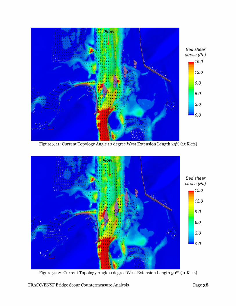
TRACC/BNSF Bridge Scour Countermeasure Analysis Page 38
Figure 3.11: Current Topology Angle 10 degree West Extension Length 25% (10K cfs)
Figure 3.12: Current Topology Angle 0 degree West Extension Length 50% (10K cfs)
Flow
Flow

TRACC/BNSF Bridge Scour Countermeasure Analysis Page 39
3.3. Design of Extension Orientation
As previously discussed, the pier extensions with their streamlined wedge shape are not at
risk for the type of local scour that develops at bluff body piers in the flow. There is, however, a
risk of local scour starting at the nose tip caused by flow separation at the tip when there is a large
angle of attack in the approach flow. The orientation of the pier extensions should therefore be
designed to minimize this risk by minimizing angle of attack for flood conditions that create the
greatest scour risk, the 30,000 cfs flood.
The first simulations with the originally proposed 200 foot pier extensions with the
provided orientation indicated that the approach flow was not aligned with the pier extensions.
They were pointed a bit east of the approach flow. To test variations of the orientation of the pier
extensions, cases with the pier extensions rotated 0 degrees, 5 degrees, 10 degrees, and 15 degrees
to the west from the original position were run. The rotation was done about the right corner of
the base as shown in Figure 3.13. The angle of attack of the approach flow is measured along the
centerline of the pier extension nose. If the approach flow velocity vector just beyond the nose is
at a positive angle with respect to the line of the nose, the angle of attack is considered to be
positive, and it is considered to be negative if its angle with respect to the line of the nose is
negative, as illustrated on the left side of Figure 3.13.
Eastward rotation of the pier extensions were not tested because the west most pier
groups, 4 and 5, that have the low flow channel between them, are most at risk for scour. They are
at the lowest elevation and the largest volume of flood flow water goes past those two pier groups.
In addition to increasing an already positive angle of attack, an eastward rotation would divert
more water toward the westward piers at greatest risk.
In general, test cases that align the flood flow with the pier extensions, yielding a smaller
angle of attack, have a lower bed shear than those with larger angle of attack. A 10 degree west
rotation appeared to perform best in reducing shear stress and yielded the smallest angle of attack
for the orientations tested. For the 200 foot extension length, a rotation of 15 degrees west was
not possible for the existing topology because pier extension 4 then blocked the low flow channel,
and that test failed to converge. Two tests cases were run with a 15 degree west rotation of 100
foot extensions, and the performance appeared worse than with the ten degree rotation. Only one
test was run with a 5 degree rotation because the 10 degree rotation appeared to perform better.
Tests with two redesigned guide walls did not use a 5 degree rotation to save on effort, computer
resources, and time.
Table 2 shows the angle of attack just off the nose of the pier extensions for a variety of
conditions for the two redesigned guide walls. These were chosen from the case table to illustrate
some of the cases varying pier extension angle that can be compared for the 1st and 2nd redesigns
of the west guide wall. Small angles of attack are a good indicator of optimum orientation, with
the possible exception of west most pier extension, which will be discussed below. Angles of attack
lower than 10 degrees are likely fine, angles of attack close to or greater than 20 degrees, either
positive or negative are likely problematic. Achieving a small angle of attack in the 30,000 cfs
flood was judged the be a higher priority than for the 10,000 cfs flood because the 30,000 cfs
flood is the one that creates a scour risk that endangers the railroad bridge. The 10,000 cfs flood
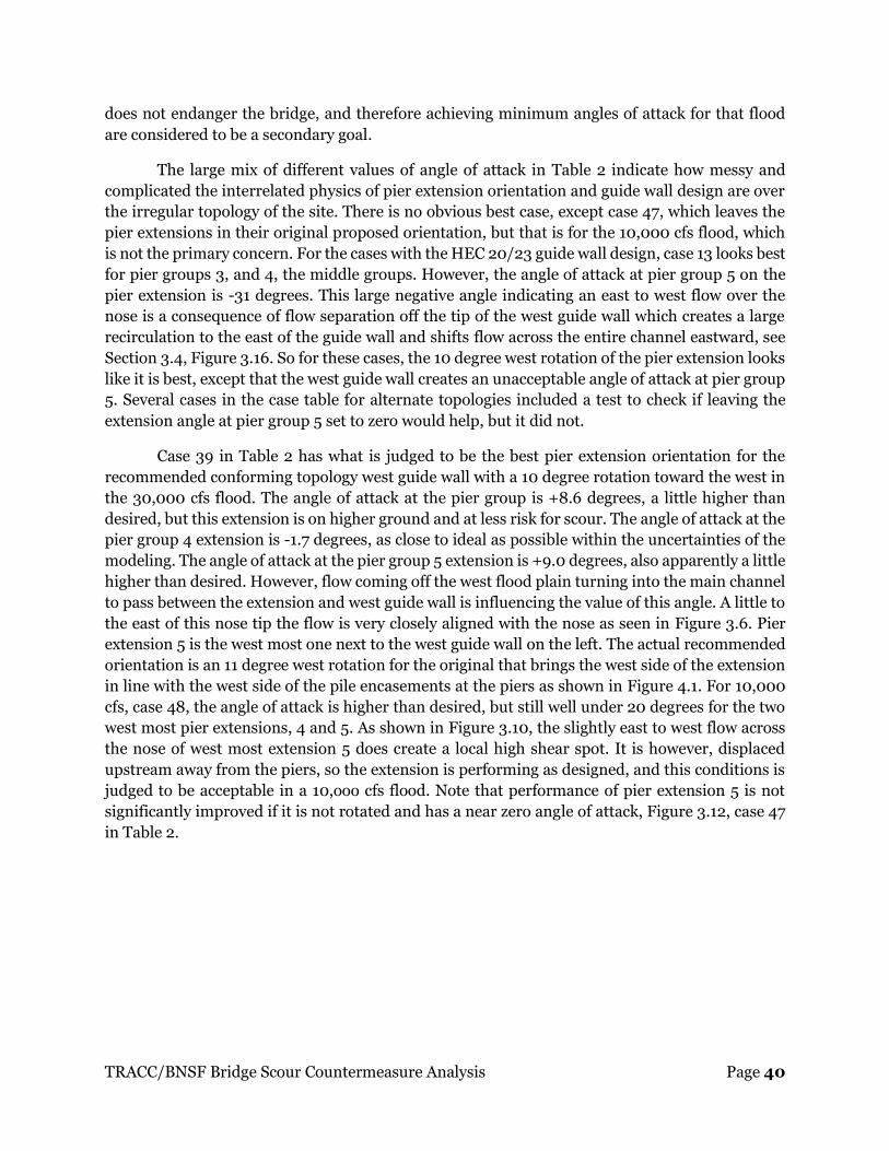
TRACC/BNSF Bridge Scour Countermeasure Analysis Page 40
does not endanger the bridge, and therefore achieving minimum angles of attack for that flood
are considered to be a secondary goal.
The large mix of different values of angle of attack in Table 2 indicate how messy and
complicated the interrelated physics of pier extension orientation and guide wall design are over
the irregular topology of the site. There is no obvious best case, except case 47, which leaves the
pier extensions in their original proposed orientation, but that is for the 10,000 cfs flood, which
is not the primary concern. For the cases with the HEC 20/23 guide wall design, case 13 looks best
for pier groups 3, and 4, the middle groups. However, the angle of attack at pier group 5 on the
pier extension is -31 degrees. This large negative angle indicating an east to west flow over the
nose is a consequence of flow separation off the tip of the west guide wall which creates a large
recirculation to the east of the guide wall and shifts flow across the entire channel eastward, see
Section 3.4, Figure 3.16. So for these cases, the 10 degree west rotation of the pier extension looks
like it is best, except that the west guide wall creates an unacceptable angle of attack at pier group
5. Several cases in the case table for alternate topologies included a test to check if leaving the
extension angle at pier group 5 set to zero would help, but it did not.
Case 39 in Table 2 has what is judged to be the best pier extension orientation for the
recommended conforming topology west guide wall with a 10 degree rotation toward the west in
the 30,000 cfs flood. The angle of attack at the pier group is +8.6 degrees, a little higher than
desired, but this extension is on higher ground and at less risk for scour. The angle of attack at the
pier group 4 extension is -1.7 degrees, as close to ideal as possible within the uncertainties of the
modeling. The angle of attack at the pier group 5 extension is +9.0 degrees, also apparently a little
higher than desired. However, flow coming off the west flood plain turning into the main channel
to pass between the extension and west guide wall is influencing the value of this angle. A little to
the east of this nose tip the flow is very closely aligned with the nose as seen in Figure 3.6. Pier
extension 5 is the west most one next to the west guide wall on the left. The actual recommended
orientation is an 11 degree west rotation for the original that brings the west side of the extension
in line with the west side of the pile encasements at the piers as shown in Figure 4.1. For 10,000
cfs, case 48, the angle of attack is higher than desired, but still well under 20 degrees for the two
west most pier extensions, 4 and 5. As shown in Figure 3.10, the slightly east to west flow across
the nose of west most extension 5 does create a local high shear spot. It is however, displaced
upstream away from the piers, so the extension is performing as designed, and this conditions is
judged to be acceptable in a 10,ooo cfs flood. Note that performance of pier extension 5 is not
significantly improved if it is not rotated and has a near zero angle of attack, Figure 3.12, case 47
in Table 2.

TRACC/BNSF Bridge Scour Countermeasure Analysis Page 41
Table 2: Angle of Attack for HEC 20/23 West Guide Wall
Case no.
Topology Extension
Length Guide wall
type
Extension Angle
(α deg)
Flow Angle of Attack (degree)
Flood
Pier-3 Pier-4 Pier-5 Discharge
11 Existing 50%
(~100ft) HEC 20/23 0 16.6 13.9 -12.4 30k cfs
13 Existing 50%
(~100ft) HEC 20/23 10 -6.57 -7.31 -31.15 30k cfs
15 Existing 50%
(~100ft) HEC 20/23 15 -14.9 -19 -34.9 30k cfs
47 Existing 50%
(~100ft) HEC 20/23 0
No flow
-16.6 18.9 10k cfs
39 Existing 50%
(~100ft) topology
conforming 10 8.6 -1.68 9.03 30k cfs
47 Existing 50%
(~100ft) topology
conforming 0
No flow
-1.2 -2 10k cfs
48 Existing 50%
(~100ft) topology
conforming 10
No flow
-12.79 -13.14 10k cfs
Figure 3.13: Schematic showing pier-extensions approach flow angle of attack

TRACC/BNSF Bridge Scour Countermeasure Analysis Page 42
3.4. Design of West Guide Wall
The recommended design of the west guide wall was reached through two redesigns. The
initial proposed guide wall, first redesign, and final recommended design are shown side by side
in Figure 2.14. The original proposed west guide wall design as shown in the figure has a sharp
short expansion bend at the bottom southern end, however most of its length under the bridge
was straight with a slight westward curve near the northern end at the top of the figure. In the
first set of simulations with varied pier extension lengths and angles, flow separation occurred off
the northern tip of this guide wall. The flow off the golf course flood plain was shifted eastward in
bypassing the recirculation zone created by the flow separation, and a high shear patch was
present on the bed from the wall tip extending across the downslope from the flood plain into the
main channel between the wall and pier group 5.
The first redesign using guidelines in HEC 20/23 [6, 7] yielded a guide wall curving 60
feet westward over a 150 foot upstream length from the midpoint under the bridge. This shape is
intended to avoid separation from the wall as a wider flow is funneled into a narrower opening
under the bridge. Results of a simulation with the recommended pier extension length and
orientation are shown in the color plotted bed shear stress map in Figure 3.16 for 30,000 cfs flood
conditions. Velocity direction vectors for flow just above the bed are also shown. While this design
might work well for a relatively flat topology where the incoming flow including that on the flood
plain does not extend laterally beyond the upstream tip of the wall, it clearly did not work well for
the site conditions at the BNSF bridge. Enough water on the flood plain flows behind the wall on
the west, the right side of this figure, it must circle back around the wall to flow under the bridge
to flow onward downstream. As a result, flow separation off the upstream tip of the wall still
occurs, and even though the tip is farther west on the flood plain, the recirculation zone on the
channel side of the wall still extends a large distance from the wall into the high flow channel.
The failure of this design to solve the separation problem prompted a more detailed
consideration of the local topology at the site to be used in the west guide wall design. A view of
the local topology is shown in Figure 3.14 with patches of high ground on the golf course flood
plain to the west labeled along with lower lying flow paths off of the flood plain. Two of these lower
lying flow paths appear to be golf cart paths just north of the railroad. The elevations are color
plotted in Figure 3.15, and it is easy to see there the topology elevation variations of the golf course
flood plain to the west. The recommended guide wall is also shown in the figure. It curves around
the northern side of the first patch of high ground north of the railroad allowing flow to come off
the flood plain down the golf cart path running between the patches of high ground. It was
extended far enough west up onto the flood plain to prevent large amounts of flow over the flood
plain to go behind it. Three dimensional CFD was well suited to testing this design because it can
solve for the effect of the variations in elevation over the local topology on the flow. A concern
with this design was that the tighter curvature in this design might result in separation of flow
from the wall, not solving that problem.

TRACC/BNSF Bridge Scour Countermeasure Analysis Page 43
Figure 3.14: Image showing topology of channel and flood plane
Source: Riverside county, CA, 33°52'30.83" N and 117°40'02.92" W. Google Earth. April 4,
2014. Accessed: March 03, 2015.
Figure 3.15: Topology Conforming Guide Wall Design
Many of the figures in other sections show shear stress color plots with the recommended
guide wall design. For purposes of comparison with the performance of the other guide wall
N
E
Flow

TRACC/BNSF Bridge Scour Countermeasure Analysis Page 44
designs in 30,000 cfs flood flow conditions, Figure 3.17 shows a color plot of bed shear with the
same orientation, the primary flow direction is from bottom to top, as the previous two figures.
While there is what looks like a thin separated layer near the west tip of the wall, the big
recirculation zone resulting from separation off the tip from the two earlier designs is gone, and
the velocity direction vectors plotted just off the bed show flow moving smoothly off the flood
plain to join the main flow between pier group 5 and the west guide wall. There are still patches
of high shear spots on the flood plain that are likely a consequence of the elevation variations.
Note that the high shear patch off the west side of the tip of pier group extension 5, due to the
shifted angle of attack caused by the recirculation zone from the HEC 20/23 guide wall design, in
Figure 3.16 is also gone.
Under lower flow rate conditions, the west guide wall design is not as important because
it is the 30,000 cfs flood that creates the primary risk of a scour failure at the BNSF bridge. Figure
3.10 shows the shear stress for a worst case scenario for a 10,ooo cfs flood. Water depth was
adjusted to achieve higher velocity at the bridge than would likely be the case with field conditions.
In this case there is not much flow reaching the west guide wall and the flow is primarily straight
down the low flow channel direction, which causes flow separation off the nose of the pier group
5 extension and a high shear patch there. If this were to occur, the extension is functioning as
intended by displacing a potential scour location upstream of the railroad piers, and scour near
the pier extension tip would deepen the channel at that location dropping the shear stress.
A west guide wall design that conforms to the local topology of the golf course flood plain
performs very well in the CFD case tests and is the recommended design. It guides flow off the
flood plain and serves to contract it smoothly into the flow under the bridge in cases where there
is significant flow on the west flood plain.
High shear stress areas on the bed can be caused by flow over changing topology, often
near a rise in bed elevation, as well as flow separation and contraction at the structures in the
flow. Most of the high shear area in these plots is primarily a consequence of variations in the
topology.

TRACC/BNSF Bridge Scour Countermeasure Analysis Page 45
Figure 3.16: HEC 20/23 based guide wall, 30K cfs flood, and existing topology
Figure 3.17: Topology conforming guide wall, 30K cfs flood
Flow
Flow

TRACC/BNSF Bridge Scour Countermeasure Analysis Page 46
Figure 3.18: Dye visualization of flow at west guide wall in physical model test of 30K cfs flood
Figure 3.18 shows the topology conforming west guide wall functioning very well in the
physical model at the USACE ERDC facility. The upper pictures and lower picture on the right
show dye injected both behind the guide wall on the right and in front of the guide wall on the
right. The flow on the west flood plain is proceeding from right to left up to the guide wall. The
guide wall is guiding the flow back toward the main channel to flow under the bridge, out of the
pictures beyond the bottom of the frames. While there is a little separation at the tip of the wall,
the separated zone is thin and short, and the dye follows the contour of the wall very closely as
intended in the design. The last frame on the lower right shows dye flow pattern for dye injected
behind the wall. This flow is returning flow from water higher up off of the frames that bypassed
the wall farther to the west. Its volume flow rate is low enough that it does not create significant
separation off the tip of the wall, and it follows the contour of the wall closely back to the main
channel as intended.
3.5. Performance of Pier Extensions with Alternate Topologies
Pier extension and guide wall performance in achieving a relatively low bed shear stress
in the near vicinity of the bridge piers was checked for three alternate topologies. These topologies
were constructed to see what could happen in the domain of the bridge once the channel has
undergone long term degradation scour. A large 300 foot westward migration of the channel

TRACC/BNSF Bridge Scour Countermeasure Analysis Page 47
without degradation was also created to test the effect of change in angle of attack due to channel
migration.
3.5.1. Long Term Degradation Scour with Wide Channel
A long term degradation scour wide channel geometry was developed assuming
meandering over a long period of time would lower the channel to the degradation scour elevation
projection across the full width of the bridge between the four sets of piers between guide walls as
described in Section 2.2. Figure 3.19 shows bed shear stress for this wide channel degradation
scour topography with pier extensions. In this case, the uniform degradation assumption leads to
significant increase in flow cross section area, resulting in lower flow average velocity, and hence
lower bed shear stresses. Further, there is scarcely any flow away from the channel in the west
flood plain. Nearly all of the water flow is contained in the main flow channel. For this topology,
further degradation of channel should be a slow process because bed shear stress caused by
30,ooo cfs flood conditions is relatively low for such channel shape. This topology is judged to be
not likely to develop under real conditions. Much more likely, long term degradation scour will
produce a narrow channel similar to the existing low flow channel but at the degradation scour
elevation as described in Section 2.2.
Figure 3.19: Long term uniform degradation scour wide channel
Flow

TRACC/BNSF Bridge Scour Countermeasure Analysis Page 48
3.5.2. Long Term Degradation Scour with a Narrow Low Flow Channel
A long term degradation scour topology with a narrow low flow channel migrated a
maximum of 100 foot west was developed described in Section 2.2. Figure 3.20 and Figure 3.21
show bed shear stress for the recommended pier extension length and both the original
orientation and the 10 degree west extension rotation. These cases were run with the first redesign
of the west guide wall and were not repeated after the second redesign. As described in Section
2.2, this topology consists of a narrow scoured channel with deepest point at 392 foot elevation
about 16 feet lower than current topology. The bed shear stress is much lower than in the existing
topology cases. However, how much of this reduction may be due to the stress reduction from
contraction scour and how much is a consequence of the choice of channel cross section profile,
is difficult to say.
Figure 3.20: Narrow channel long term degradation scour topology with 0 degree west
extension orientation and 100 foot length
Flow
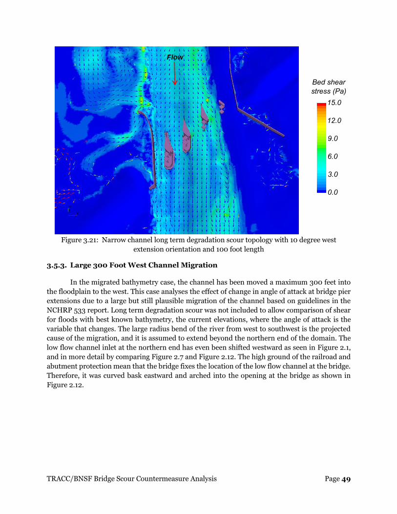
TRACC/BNSF Bridge Scour Countermeasure Analysis Page 49
Figure 3.21: Narrow channel long term degradation scour topology with 10 degree west
extension orientation and 100 foot length
3.5.3. Large 300 Foot West Channel Migration
In the migrated bathymetry case, the channel has been moved a maximum 300 feet into
the floodplain to the west. This case analyses the effect of change in angle of attack at bridge pier
extensions due to a large but still plausible migration of the channel based on guidelines in the
NCHRP 533 report. Long term degradation scour was not included to allow comparison of shear
for floods with best known bathymetry, the current elevations, where the angle of attack is the
variable that changes. The large radius bend of the river from west to southwest is the projected
cause of the migration, and it is assumed to extend beyond the northern end of the domain. The
low flow channel inlet at the northern end has even been shifted westward as seen in Figure 2.1,
and in more detail by comparing Figure 2.7 and Figure 2.12. The high ground of the railroad and
abutment protection mean that the bridge fixes the location of the low flow channel at the bridge.
Therefore, it was curved bask eastward and arched into the opening at the bridge as shown in
Figure 2.12.
Flow

TRACC/BNSF Bridge Scour Countermeasure Analysis Page 50
Figure 3.22: Shear stress for extension angle 10 degree west, extension length 50% (~100ft.)
with topology conforming guide wall (33K cfs)
In case of the 190 year (33K cfs) flood, there is no significant increase in bed shear at the
piers, although flow pattern has changed significantly as shown in Figure 3.23. There is limited
spread of water into the floodplain due to the change in channel path in approaching the bridge.
Recirculation zones form in the floodplain shifting the channel flow slightly east of flow in the
existing topology, and consequently the angle of attack shifts slightly eastward. This was not
expected, but demonstrates that the recommended design functions well if conditions shift the
angle of attack slightly to the east.
High shear stress areas on the bed are also caused by flow over changing topology, often
near a rise in bed elevation, as well as flow separation and contraction at the structures in the
flow. Most of the high shear area in these plots is primarily a consequence of variations in the
topology.
In the 10K flood, the bed shear stress is reduced in the west migrated channel due to spread
of water over a wider area compared to current bathymetry. Again, the west flood plain has
recirculation zones, and the main flow approaching the piers is coming primarily down the path
of the low flow channel, although the flow pattern is somewhat complex as seen in Figure 3.23.
Flow

TRACC/BNSF Bridge Scour Countermeasure Analysis Page 51
Figure 3.23: Angle 10 degree West Extension Length 50% (~100ft.) with Topology Conforming
Guide Wall (10K cfs)
3.6. Pressure and Shear Stress Distribution on Pier-Extensions
Figure 3.24 and Figure 3.25 show the static and dynamic pressure on the pier group 4 pier
extension, the second from the west guide wall. The maximum dynamic pressure (Figure 3.25) on
the pier extensions is nearly an order of magnitude less than the maximum static pressure (Figure
3.24). The step up from the nose to the top of the wedge of the extension has been eliminated from
the final design recommendation without rerunning the case. That change, however, will
eliminate the highest dynamic pressure, which is only 1.4 psi, on the front of the wedge. Pressures
between 1.2 and 1.4 psi are seen on the right side of the pier extension due to the angle of attack
of the approach flow.
Flow
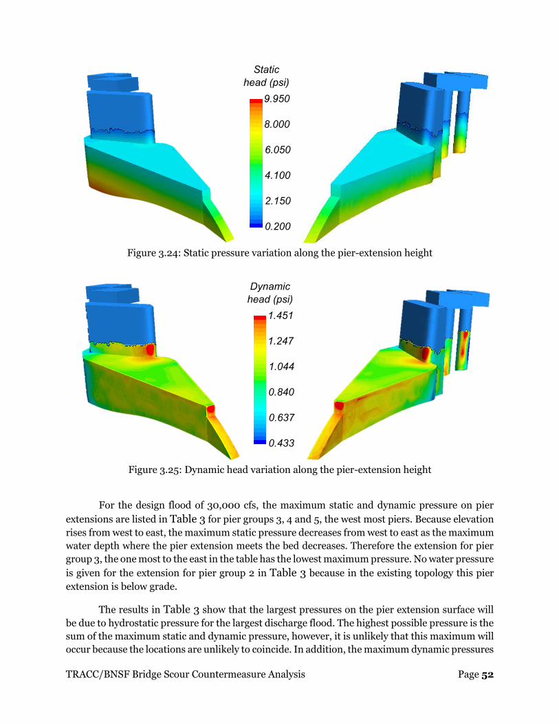
TRACC/BNSF Bridge Scour Countermeasure Analysis Page 52
Figure 3.24: Static pressure variation along the pier-extension height
Figure 3.25: Dynamic head variation along the pier-extension height
For the design flood of 30,000 cfs, the maximum static and dynamic pressure on pier
extensions are listed in Table 3 for pier groups 3, 4 and 5, the west most piers. Because elevation
rises from west to east, the maximum static pressure decreases from west to east as the maximum
water depth where the pier extension meets the bed decreases. Therefore the extension for pier
group 3, the one most to the east in the table has the lowest maximum pressure. No water pressure
is given for the extension for pier group 2 in Table 3 because in the existing topology this pier
extension is below grade.
The results in Table 3 show that the largest pressures on the pier extension surface will
be due to hydrostatic pressure for the largest discharge flood. The highest possible pressure is the
sum of the maximum static and dynamic pressure, however, it is unlikely that this maximum will
occur because the locations are unlikely to coincide. In addition, the maximum dynamic pressures

TRACC/BNSF Bridge Scour Countermeasure Analysis Page 53
given in the table are on the step up from the downward sloping pier extension nose to the pier
extension wedge, which, as noted previously, has been removed from the final design. Therefore
these maximum dynamic pressures are conservative for this case.
Table 3: Pressure on Pier-Extensions for 30,000 cfs Flood
Pier-extension
group
Max dynamic pressure
(psi)
Max hydrostatic pressure
(psi)
3 1.59 5.62
4 1.62 9.05
5 1.42 9.65
The shear stress distribution on the pier group 4 pier extension is shown in Figure 3.26
for the design flood of 30,000 cfs and the maximum shear stress on the above grad extensions
that are exposed to the flow is given in Table 4. These stresses are nearly three orders of
magnitude less that the maximum hydrostatic pressure on the extensions in the 30,000 cfs flood.
Figure 3.26: Shear stress on the pier-extension surface
Table 4: Shear Stress on Pier-Extensions for 30,000 cfs Flood
Pier-extension group Shear Stress (psi)
3 3.77E-03
4 4.68E-03
5 4.14E-03

TRACC/BNSF Bridge Scour Countermeasure Analysis Page 54
4. Recommended Design for Pier Extensions and West Guide
Wall
The recommended design parameters meet the primary goals of the project for varied
conditions that exist now at the site and may develop over time. However, the recommended
designs may not be the best for any particular condition. The recommended designs are based on
both qualitative and quantitative information learned about flood flow behavior in the system
under a variety of flow conditions through CFD analysis. The quantitative results provide the
easiest basis for design decisions. The qualitative results provide physical insights for engineering
judgment that has developed over many years of experience and can therefore be very good. For
both types of information, minimization of scour at the piers for the 30,000 cfs flood carries the
most weight because that flow with the predicted long term degradation scour is the one that poses
the risk of pier and bridge failure. The following recommendations are based on the fifty plus CFD
analysis case runs in combination with engineering judgment.
The recommended pier extension length is ~100 feet, 50% of original design
The recommended pier extension design configuration is shown in Figure 4.1. The length
provides sufficient displacement of local scour risk on the upstream side of the piers to a position
where a scour hole that may develop at the extension nose tip will not impact the railroad piers.
The narrow, down-sloping nose at the upstream end of the wedge shaped, streamlined extensions
also minimize the possibility of a scour hole of significant depth forming at the nose.
Pier extensions of about 50 feet in length, 25% of original design length were judged to be
too short to provide an adequate safety margin for larger scour holes that could develop at the
pier nose extension tips in the low probability case that future conditions produce flood flows with
very large angles of attack.
The gap between the end of the pier extensions and the semi-rectangular
piers should be closed
As shown in Figure 4.1, a pier extension ends along a diagonal line at the upstream end of
the pile enclosure, and the pier extension height extends about half of the semi-rectangular pier
height above the top of the pile enclosure, potentially leaving a gap between the downstream end
of the pier extension and the upstream end of the semi-rectangular piers. This gap should be
closed. Early simulations extensions showed that flow through the gap can increase bed shear at
the base of the semi-rectangular piers, making the shielding effect of the pier extensions
incomplete. All simulations with pier extensions that were used to reach the other design
recommendations were done with the gap between pier extensions and the semi-rectangular piers
closed.

TRACC/BNSF Bridge Scour Countermeasure Analysis Page 55
Figure 4.1: Recommended Bridge Pier Extension Configuration – Side and Top Views
The recommended angle for pier extensions is ~11 degrees west of original
design
The desired angle is a zero degree angle of attack in flood flows. The 30,000 cfs flood has
significant flow coming off the west flood plain, and the 11 degree west orientation yields an angle
of attack very close to zero in the full scale computational domain. It might be slightly off due to
trees, vegetation, and other small features not included in the model, but it should be close to the
goal of a minimum angle of attack at the site under the 30,000 cfs flood conditions. The angle was
chosen for this flood because it is the one that poses a failure risk at the piers for the current
conditions with no pier extensions.
The 10,000 cfs flood has much lower flow off the west flood plain, and the change in angle
of attack does increase scour risk at pier group 5 due to separation off the pier extension nose.
That scour would occur upstream on the upslope elevation of the west bank of the channel in low

TRACC/BNSF Bridge Scour Countermeasure Analysis Page 56
flow. It may be slowed by vegetation, and to the extent that it does occur it would widen the
channel causing a drop in bed shear to a point where the scour stops before reaching the bridge.
The topology conforming west guide wall works best and is recommended
The original west guide wall design and the first redesign based of the guidelines of HEC
20/23 blocked flow moving off the west flood plain. The flow behind the wall then circled around
behind the wall coming back around with a large separation angle off the tip. This separated flow
created a large separated flow zone on the channel side of the wall that effectively narrowed the
flow through width of the channel making conditions worse.
The topology conforming guide wall was designed to avoid blocking the primary low lying
natural flow paths off of the flood plain, and this design was found to have minimal separation
from the wall for the 30,000 cfs flood. For the 10,000 cfd flood, there is no significant flow off of
the flood plain at the west guide wall. The recommended west guide wall design is shown in Figure
4.2.
Figure 4.2: Recommended design for topology conforming guide wall

TRACC/BNSF Bridge Scour Countermeasure Analysis Page 57
The final designs of scour countermeasures at the bridge recommended for testing in the physical
model are shown together in Figure 4.3. The differences from the original proposed design before
refinement based on 3D CFD analysis are (1) a 50% reduction in extension length to about 100
feet, (2) an orientation of the extensions shifted about 11 degrees westward to minimize the angle
of attack at the pier extension noses in the 30,000 cfs flood, and (3) a west guide wall curving and
extending a much larger distance westward into the west flood plain that conforms to the local
topology and guides most of the water coming off of the west flood plain smoothly back into the
main channel at the bridge opening. While not shown in the figure, closure of the gap between the
pier extensions and the rectangular piers is also an important component of the refined design
recommendations, as noted in one of the recommendations above.
Figure 4.3: Final recommended design including optimized pier-extensions and guide walls
based on CFD analysis

TRACC/BNSF Bridge Scour Countermeasure Analysis Page 58
5. References
[1] Hogan, S; Kerenyi, K. Santa Ana River, Reach 9, BNSF Railroad Bridge, Bridge Hydraulics
and Scour Analysis Review [Memorandum]. Federal Highway Administration, March
2014
[2] Evaluating Scour at Bridges, Fifth Edition, Hydraulic Engineering Circular No. 18, U.S.
Department of Transportation Federal Highway Administration, April 2012
[3] Livermore Software Technology Corporation LS-PrePost Online documentation,
http://lstc.com/lspp, Last accessed: March 2015
[4] MeshLab an Open Source System for Processing and Editing Unstructured 3D Triangular
Meshes http://meshlab.sourceforge.net/, Last accessed: March 2015
[5] Lower Santa Ana River, Reach 9, Burlington Northern and Santa Fe Railroad Bridge
(Scour Protection), Design Documentation Report, Los Angeles District, Corps Of
Engineers
[6] Sharp, J.A. and Heath, R.E., Two-Dimensional Model Study of Santa Ana River Railroad
Bridge Pier Extensions, ERDC/CHL Letter Report, US Army Corps Of Engineers, January
2014
[7] CD-adapco, User Guide STAR-CCM+ Version 9.06, 2014
[8] US Army Corps of Engineers, “HEC-RAS River Analysis System, Applications Guide
Version 4.1,” Hydrologic Engineering Center, January 2010
[9] Stream Stability at Highway Structures, Fourth Edition, Hydraulic Engineering Circular
No. 20, U.S. Department of Transportation Federal Highway Administration, April 2012
[10] Bridge Scour and Stream Instability Countermeasures, Experience, Selection, and Design
Guidance, Second Edition, Hydraulic Engineering Circular No. 23, U.S. Department of
Transportation Federal Highway Administration, March 2001
[11] Handbook for Predicting Stream Meander Migration, NCHRP REPORT 533,
Transportation Research Board, Washington, D.C., 2004
[12] Rodi, W., Experience with Two-Layer Models Combining the k-e Model with a One-
Equation Model Near the Wall, 29th Aerospace Sciences Meeting, AIAA-91-0216, Reno,
NV, 1991
[13] Shih, T.; Liou, W.; Yang, Z.; and Zhu, J.; A New k-Eddy Viscosity Model for High Reynolds
Number Turbulent Flows – Model Development and Validation. Institute for

TRACC/BNSF Bridge Scour Countermeasure Analysis Page 59
Computational Mechanics in Propulsion Center for Modeling of Turbulence and
Transition. Cleveland, OH: NASA Lewis Research Center, 1994
[14] Patankar, S.V., Numerical Heat Transfer and Fluid Flow, McGraw-Hill, 1980
[15] Launder, B.E. and Spalding, D.B., The Numerical Computation of Turbulent Flows,
Computer Methods in Applied Mechanics and Engineering, 3, 1974

Energy Systems Division
Argonne National Laboratory
9700 South Cass Avenue, Bldg. 362
Argonne, IL 60439-4815
www.anl.gov
Argonne National Laboratory is a U.S. Department of Energy
laboratory managed by UChicago Argonne, LLC


