This document contains the draft version of the following paper: R.M. Gouker, S.K. Gupta, H.A. Bruck, and T. Holzschuh. Manufacturing of multi-material compliant mechanisms using multi-material molding. International Journal of Advanced Manufacturing Technology, 30(11-12):1049-1075, 2006. Readers are encouraged to get the official version from the journal’s web site or by contacting Dr. S.K. Gupta ([email protected]).
Manufacturing Of Multi-Material Compliant Mechanisms Using Multi-Material Molding
Regina M. Gouker, Satyandra K. Gupta, Hugh A. Bruck, and Tobias Holzschuh
Mechanical Engineering Department
University of Maryland
College Park, MD 20742
AbstractMulti-material compliant mechanisms enable many new design possibilities. Significant progress has been made in the area of design and analysis of multi-material compliant mechanisms. What is now needed is a method to mass-produce such mechanisms economically. A feasible and practical way of producing such mechanisms is through multi-material molding. Devices based on compliant mechanisms usually consist of compliant joints. Compliant joints in turn are created by carefully engineering interfaces between a compliant and a rigid material. This paper presents an overview of multi-material molding technology and describes feasible mold designs for creating different types of compliant joints found in multi-material compliant mechanisms. It also describes guidelines essential to successfully utilizing the multi-material molding process for creating compliant mechanisms. Finally, practical applications for the use of multi-material molding to create compliant mechanisms are demonstrated.
Keywords: Compliant mechanisms, compliant joints, multi-material molding, and mold design.
1
1 Introduction
Synthetic and natural structures have several distinct differences. Perhaps the greatest difference between these two types of structures is the use of compliance. Compliance, in relation to structures and mechanisms, is the ability or process of yielding to changes in force without disruption of structure or function. It has been well recognized that man-made objects are primarily made up of relatively rigid materials, while natural objects are made with soft compliant materials, using rigid materials such as bones and teeth only in select places [Vogel, 1995]. It has been suggested that this distinct difference occurs from the assembly and production methods for each of the products. The fundamental requirement for natural structures is the absence of assembly. The entire system must be grown from a source or cell as a single entity [Ananthasuresh and Kota, 1995].
An example of the type of unique performance that can be achieved through the use of compliance in natural structures is the flapping of bird wings to achieve flight (Figure 1). It has been shown that birds are designed with an integrated flexibility to promote draft and lift, caused by the air, to rotate the wings throughout the cyclic process [Vogel, 1995]. This enables the bird to achieve much higher cyclic flapping rates at lower energy consumption.
A common misconception is that an object has to be rigid to be strong [Vogel, 1995]. However, nature shows us that objects can be strong and compliant. Throughout human existence, nature has proven to be a fertile source for inspiration. Until recent years, many of these ideas could never be fully understood and reconstructed. With an improved understanding of the structure-property-function relationship in biological materials and systems and the invention of new materials and manufacturing techniques, bio-inspired designs are rapidly increasing in popularity [Goldin et al., 2000].
In a step towards bio-inspired design, the behavior of compliant mechanisms has been studied in order to develop design rules for realizing actual mechanisms. A compliant mechanism is a flexible structure that elastically deforms to produce desired force or displacement. Similar to rigid mechanisms, compliant mechanisms will still transfer or transform motion, force, or energy, but they will also store strain energy in the flexible members as well [Howell, 2001]. Compliant mechanisms mainly consist of rigid objects or features with added compliant or soft materials at strategic locations. There are several different types of compliant mechanisms currently being researched and developed. Some of the mechanisms developed include bistable mechanisms, ortho-planar flat spring, centrifugal clutches, over-running pawl clutches, near-constant-force compression mechanisms, near-constant-force electrical connectors, bicycle brakes, bicycle derailleur, compliant grippers and microelectromechanical systems [Howell, 2001].
Compliant designs have many advantages over traditional designs that employ articulated joints. Included in these advantages is the reduction of wear between joint members, reduction in backlash and high potential energy stored in deflected members [Howell et al., 1996]. In addition, absence of assembly in production methods, reduction of weight and part count found in compliant mechanisms all lead to the reduction of cost to manufacture the product. Several studies have indicated that assembly costs make up 40% to 50% of the manufacturing costs to produce a product [Ananthasuresh and Kota, 1995]. Part reduction reduces the assembly labor, purchasing, inspecting, warehousing, capitol requirements and piece part costs of a product
2
[Rotheiser, 2004]. Therefore any decrease in part count and manufacturing cost, no matter how minimal, will have a drastic effect on the total cost of the product.
The use of multiple different materials in compliant mechanisms opens up the design space considerably. Until recently, a method did not exist to mass produce multi-material compliant mechanisms. In the past, layered processes, such as Stereolithography, Selective Laser Sintering, Shape Deposition Modeling and 3D Printing were utilized for making multi-material compliant mechanisms [Bailey et al., 1999; Beaman et al., 2000; Jackson et al., 1998]. While these processes can create intricate and complex geometries as well as material distributions, they are not suitable for mass production in most cases. A more suitable technique that has emerged for the manufacturing of multi-material compliant mechanisms is multi-material molding. Multi-material molding creates a part with one or more materials via a multi-stage mold.
Multi-material compliant mechanisms are able to achieve the same performance as homogeneous mechanism with complex geometries because they employ compliant joints. The compliant joints are created by carefully engineering interfaces between two materials: one that is compliant and one that is rigid. This paper describes several different types of interfaces that can exist in compliant joints. Furthermore, this paper presents results from experimental characterization of these interfaces to show that these interfaces are viable for creating compliant joints with the adequate motion ranges. A detailed description for designing several different compliant joints that can provide from one to three degrees-of-freedom motions in mechanisms is outlined. For each joint design, we discuss possible mold design options and present a feasible mold design to realize the joint. Finally, we present two examples of devices consisting of compliant joints.
The material presented in this paper will assist readers in designing and experimentally analyzing molded multi-material compliant mechanisms. Furthermore, it will help them in designing molds for manufacturing compliant mechanisms. We expect that this in turn will result in a more widespread use of multi-material compliant mechanisms.
2 Multi-Material Molding
2.1 Process Overview
Multi-material molding (MMM) involves molding multi-material assemblies from various polymers including thermosets, thermoplastics, and polyurethanes [Goodship and Love, 2002; Maniscalco, 2004; Pirkl, 1998; Plank, 2002]. The general molding process entails introducing the liquid material into a cavity shaped like the desired object, then allowing the liquid to solidify through cooling or chemical reactions. The hardened object can then be removed from the mold, where it may require finishing operations before it is complete. The multi-material molding process is very similar to the standard molding process, except the multi-material process makes use of more than one cavity configuration. Examples of some products molded with MMM techniques are shown in Figure 2.
There are many different types of design options for cavity change. Out of these, we have determined that the following three are most relevant for making compliant mechanism: cavity transfer, removable core, and sliding core methods. The cavity transfer method involves transferring the first stage part into another mold cavity (Figure 3). This method simplifies mold design and many complex interfaces can easily be created. It also requires the most manipulation between stages. In the removable core method, all that is needed to transfer from
3
one stage to the next is to remove the core (Figure 4). This type of approach requires little to no manipulation between mold stages but is also very limited in the type of interfaces that can be created. In the sliding core method the total cavity of the part is extracted from the initial mold volume and sliding cores are strategically placed within the mold to restrict or enable flows into certain sections (Figure 5). This method requires minimal manipulation between mold stages, since the part remains in the same mold cavity throughout the process. It also enables more complex interface options, but is more difficult to design because of the need to accommodate the motion of the sliding cores.
Multi-material (MM) products possess several beneficial qualities over traditionally-molded products including: (1) multicolor appearance, (2) skin/core configurations, (3) in-mold assembly, (4) selective compliance, and (5) soft-touch portions. Additionally, it could cost less to produce a MM product compared to a similar assembly of multiple components.
There are two broad manufacturing technologies commonly used to make MM objects: injection molding and room temperature molding. Injection molding is commonly used for large scale production processes, while room temperature molding is primarily used for small production runs. Injection molding involves injecting molten plastic into a mold where it rapidly solidifies and is then ejected as the desired object [Malloy, 1994]. Injection molding is ideal for many applications because it is amenable to a variety of polymeric materials, has a wide range of mold capabilities—including complex structures—and is extremely controllable. Additionally, the parts produced by injection molding have a very low cycle time. Fundamentally, there are three different types of MM injection molding processes. Multi-component molding is the simplest and most common form of MM injection molding. It involves the simultaneous (or sometimes sequential) injection of two different materials through either the same or different gate locations in a single mold. Multi-shot molding (MSM) is the most complex and versatile MM injection molding process. It involves injecting the different materials into the mold in a specified sequence, where the mold cavity geometry may partially or completely change between sequences. Over-molding and insert molding simply involve molding a resin around a preformed part; either metal (as in insert molding), or a previously-made injection-molded plastic part (as in over-molding). Each of the three classes of MM injection molding processes is unique, and can be distinguished using the taxonomy shown in Figure 6.
Room temperature molding utilizes polymers that are liquids at room temperature. Instead of injecting a hot liquid into the mold and then allowing the plastic to cool into a solid, room temperature molding utilizes reactive compounds that polymerize (i.e., cure) at ambient conditions. This involves mixing two compounds, a resin and a hardener, to activate the polymer, then pouring the mixture into the mold. The material then polymerizes in the shape of the cavity. The hardening time will be considerably longer than that of injection molded plastics. Because MM objects have geometric features consisting of differing materials, the molds must be filled in stages. This means that the molds are assembled in an initial configuration and the first material stage is poured. After a specified hardening time, the molds are partially disassembled and some mold pieces are added, removed, or replaced with different ones. The second material stage can then be poured. This process is continued until all of the materials have been poured.
There are several considerations when designing MM molds for room temperature molding. As mentioned previously, they must be designed to incorporate several molding stages. Within each of these molding stages the molds must be easy and simple to manufacture, containing no
4
undercuts in them. The absence of undercuts and the inclusion of draft angles ensures ease in demolding. Finally, since there will be no pressure exerted on the molds to hold them together the parting surfaces must be designed with pins or grooves so that proper alignment may be obtained. The absence of pressure when pouring the part also has a tendency to permit the existence of air bubbles and air pockets in the mold. The strategic location of air holes can effectively eliminate a majority of these problems. Thus, the biggest difference between MM injection molding and room temperature molding is the properties of the polymers that will be employed in each of the processes. This means that the specific MMM process that is chosen for a particular MM compliant mechanism will depend on the set of material properties that are desired.
2.2 Characteristics Governing the MMM Process
This section discusses some of the characteristics that must be considered for MMM.
• Interfacial Adhesion: The phenomenon of adhesion between two materials is complex, and consequently, it is difficult to predict the nature and exact quality of the resulting interface. In particular, the strength of intermolecular bonding and mechanical interlocking will control the mechanical properties attributed to adhesion, such as interfacial strength and fracture toughness. Adhesion is a characteristic that can be engineered in the MMM process using three types of interfaces:
o Chemical Interfaces: Chemical interfaces are formed as a result of the intermolecular bonding (i.e., cross-polymerization) along the mating surface between two compatible materials. The extent and strength of the chemical interface will be governed by the curing time and the similarity of the solubility parameters for two polymers [van Krevelen, 1990]. Figure 7 shows an example of a typical molded chemical interface.
o Mechanical Interfaces: Mechanical interfaces are formed by geometrically interlocking two incompatible materials (e.g., polystyrene and polypropylene) together. Additionally, interlocking interfaces can be used to selectively control the relative movement (i.e., degrees-of-freedom) between the materials. Figure 8 shows a schematic of a bar with a mechanical interface that does not permit any relative movement between the two materials.
o Combination Interfaces: Using compatible materials at an interface with geometrically interlocking features allows components to be designed with combined interfaces that exhibit both chemical bonding and interlocking. Previous research shows that combination interfaces performed much better in tensile loading over flat bonded interfaces, which in turn, performed much better than non-bonded interlocking interfaces [Bruck et al., 2004]. This suggests when interface strength is an important consideration combined interfaces should be used.
• Rheology: Fortunately, for multi-shot molding and over molding processes, different materials flow from separate nozzles or into separate sections of the mold, meaning the actual flows never combine. In these cases, the only concern becomes whether the materials will meet along the desired interfaces and form the desired bonds or mechanical locking. This usually results in a series of equivalent standard single material injection molding flow problems that can be solved with any of the widely available mold flow simulators on the market. However, certain MMM process, such as co-injection and sandwich molding, utilize
5
flows that are actually embedded inside of each other. In these cases, flows of multiple materials must be carefully understood in order to produce suitable MM objects. However, these processes are not suitable for making multi-material compliant mechanism. Hence, from rheology point of view we can treat MMM process as sequence of single material flow problems and use established techniques from injection molding area to perform mold flow simulations.
3 Design and Characterization of Molded Multi-Material Interfaces
3.1 Processing variables
There are many variables that have an affect, either direct or indirect, on the MMM process. These parameters can be broken down into four main categories; temperature, pressure, time, and distance [Bryce, 1996]. A key parameter in MMM is the cooling time between molding stages, which affects the degree of cross polymerization at an interface. Typically, for cross polymerization to occur the second mold stage must be performed before the material has completely hardened from the first mold stage. However, the material from the first mold stage must be hardened enough so that it can be taken out from the mold. Therefore, the desire to maintain geometrically complex interfacial features directly contradicts the desire to maintain the best cross polymerization. Due to the sensitivity of the material at this critical time, it is essential to limit either the manual or robotic manipulations required between mold stages when engineering the interface. It is also necessary to design a molding schedule that balances the degree of cross-polymerization with the desire to maintain the geometrically complex interfacial features.
3.2 Interfacial Strength Characterization
To determine the effects of processing variables on the engineered interface, it is necessary to characterize the strength and deformation response of the interface. The interfacial strength will determine the critical loads for MM compliant mechanisms. To characterize the interfacial strength, it is necessary to conduct experiments to determine the critical stresses at which the interface begins to debond. For example, a recent study explored the use of complex geometry to enhance interfacial tension strength by conducting tensile tests on two-dimensional interfaces. This study found that “geometric complexity can increase the interfacial strength 20-25%”. Among the geometrically complex interfaces that were tested, it was found that circular geometries exhibited approximately 5% greater strength than rectangular geometries [Bruck et al., 2004].
There are many choices for mechanical testing of interfacial strength. However, actually conducting these tests on complete assemblies under a variety of loading conditions would be cost prohibitive. In order to circumvent this difficulty, interfacial strength can be simply determined on chemically-bonded flat interfaces under 4 different loading conditions that are locally dominant at different locations in the assembly. The 4 loading conditions are: tension, shear, peeling, and torsion.
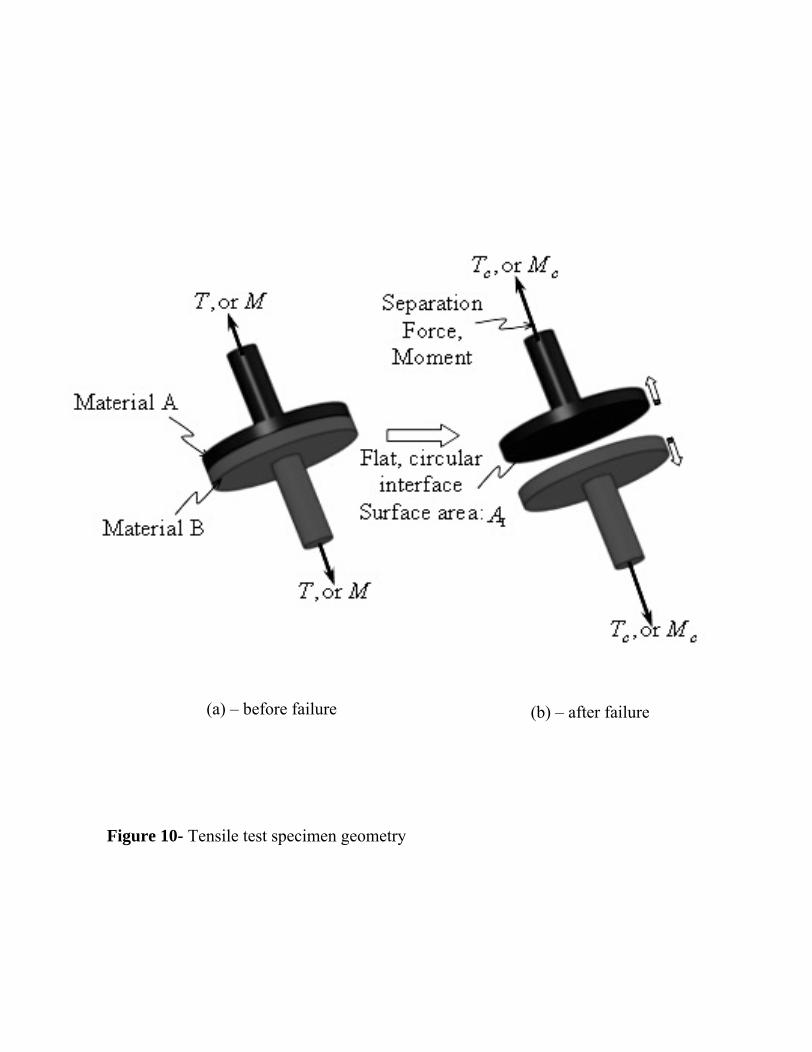
Shear and tension strengths tests measure how well the chemical interfaces resist uniform shear and normal stresses, respectively. The shear strength tests are conducted on simple lap-shear specimens, shown in Figure 9. For the tension strength tests, specimens, as illustrated in Figure 10, contain flat interfaces with circular cross-sections. In both tests, specimens pulled apart under tensile loads, and the strength determined from the critical load and interfacial area. While some
6
may argue that the two physical tests specimens discussed above are adequate to completely determine the two materials’ compatibility, it can also be necessary to conduct the peel and torsion strength tests in order to determine the chemical interface strength under gradients of normal and shear stress. The peeling test specimen is similar to the shear test specimen (Figure 9b), but is loaded with a tensile force perpendicular to the interface. The torsion strength tests utilize the same specimen testing configuration as the tensile tests, except specimens are twisted rather than pulled apart. In both cases, the geometry of the interface is used to compute the stress gradient in order to determine conditions for failure. Thus, both stress and stress gradients are used to determine interfacial failure.
A series of tension tests were conducted on the flat interface specimens seen in Figure 7 and the mechanically locking interfaces seen in Figure 8. The materials used in the test specimen are IE-70DC, a hard material, and IE-90A, a soft material (Appendix A). Typical load-displacement curves from these tests are shown in Figure 11. From these results, it can be seen that both the combination interface and the flat chemical interface have comparable mechanical responses, with the flat interface exhibiting 15% greater strength. However, when there is no chemical bonding along the interface only the mechanical interface is capable of bearing load with a strength that is 50% of the level that would be experienced with chemical bonding. Therefore, when designing with chemically compatible materials, either type of interface is suitable. However, only the mechanical interface can be used when the materials are incompatible. Both interfacial types will be employed in the case studies seen in Section 6 to demonstrate their viability using the measured strengths to set the design limits for the compliant mechanisms.
3.3 Characterizing Deformation Response of Interfaces
In addition to interfacial strength, it is also desirable to characterize the deformation response of the interface to sub-critical loads. Because of geometric complexity, it can be difficult to predict interfacial response using analytical formulas, or even Finite Element Analysis (FEA) software. In such situations, experimental characterization is the simplest and most accurate means of understanding the effects of geometric complexity on the mechanical response. Once these measurements are obtained, it may be possible to replace the geometric complexity with surrogate models containing flat interfaces of finite thickness with appropriate material properties. This will make it more reasonable to analyze assemblies with MM compliant mechanisms using commercial FEA software packages.
An example of a three-dimensional geometrically complex interface consisting of a cylindrical end with five hemi-spheres attached to the end, shown in Figure 8. This geometry was chosen based on a two-dimensional heterogeneous circular interface, fabricated with the multi-material molding process, that had been previously characterized [Bruck et al., 2004]. The analysis contains the following two tests: (1) tension test, and (2) flexure test (e.g., Cantilever Bending Test).
The materials used in the test specimen and in both of the case studies are IE-70DC, hard material, and IE-90A, soft material (Appendix A).
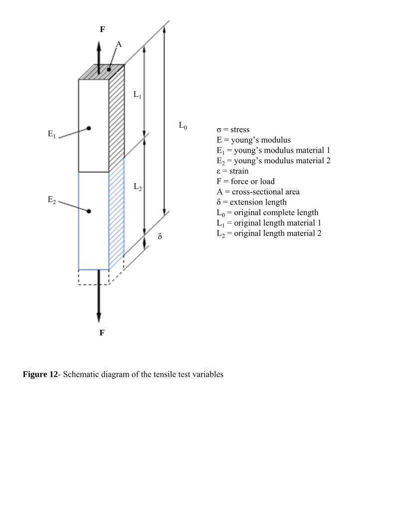
The tension test is used to determine the Young’s Modulus of each of the materials. First the specimen is stretched uniaxially, then the load and extension are measured. The axial stress is determined by dividing the load value by the specimen’s original cross-sectional area. The appropriate slope is then calculated from the stress-strain curve in the elastic region. The value of Young’s Modulus is used to calculate compliance of structural materials that follow Hooke’s law
7
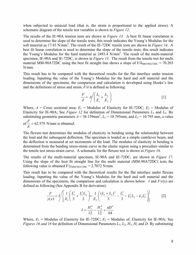
when subjected to uniaxial load (that is, the strain is proportional to the applied stress). A schematic diagram of the tensile test variables is shown in Figure 12.
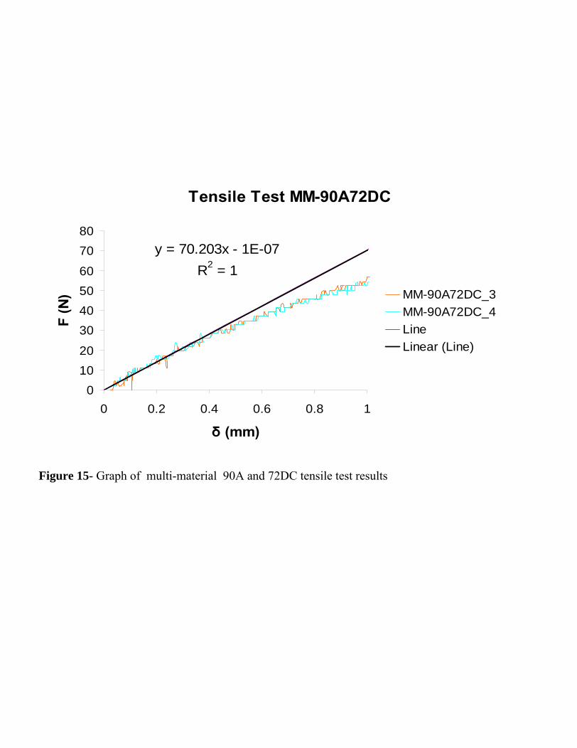
The results of the IE-90A tension tests are shown in Figure 13. A best fit linear correlation is used to determine the slope of the tensile tests; this result indicates the Young’s Modulus for the soft material as 17.83 N/mm2. The result of the IE-72DC tensile tests are shown in Figure 14. A best fit linear correlation is used to determine the slope of the tensile tests; this result indicates the Young’s Modulus for the hard material as 2493.4 N/mm2. The result of the multi-material specimen, IE-90A and IE-72DC, is shown in Figure 15. The result from the tensile test for multi material MM-90A72DC using the best fit straight line shows a slope of F/δMM-90A72DC = 70.203 N/mm.
This result has to be compared with the theoretical results for the flat interface under tension loading. Inputting the value of the Young’s Modulus for the hard and soft material and the dimensions of the specimens, the comparison and calculation is developed using Hooke’s law and the definitions of stress and strain. F/δ is defined as following:
⎟⎟⎠
⎞⎜⎜⎝
⎛+=
2
2
1
1
EL
ELAF
δ [1]
Where, A = Cross sectional area; E1 = Modulus of Elasticity for IE-72DC; E2 = Modulus of Elasticity for IE-90A; See Figure 12 for definition of Dimensional Parameters L1 and L2. By substituting geometric parameters A = 38.159mm2, L1 = 10.795mm, and L2 = 10.795 mm, a value
of 579.62=δF N/mm is obtained.
The flexure test determines the modulus of elasticity in bending using the relationship between the load and the subsequent deflection. The specimen is loaded as a simple cantilever beam, and the deflection is measured at set increments of the load. The modulus of elasticity in bending is determined from the bending stress-strain curve in the elastic region using a procedure similar to the tensile test stress-strain curve. A schematic for the flexure test is shown in Figure 16.
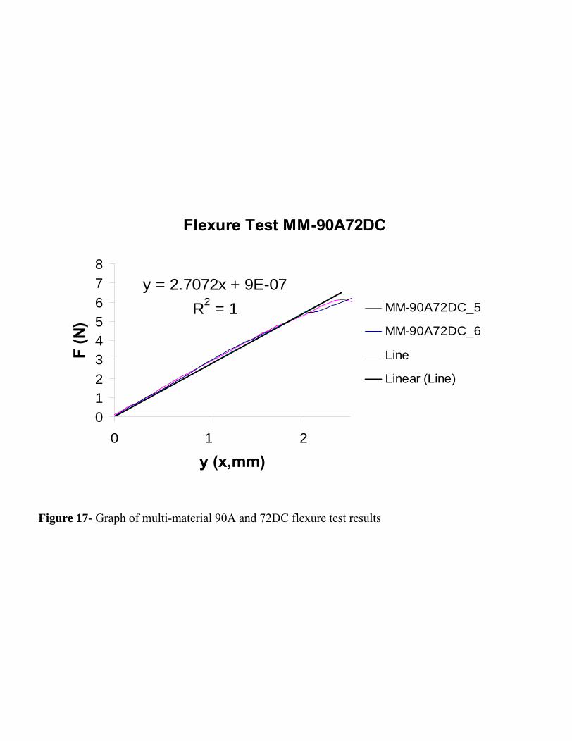
The results of the multi-material specimen, IE-90A and IE-72DC, are shown in Figure 17. Using the slope of the best fit straight line for the multi material (MM-90A72DC) tests the following value is obtained F/yMM-90A72DC = 2.7072 N/mm.
This result has to be compared with the theoretical results for the flat interface under flexure loading. Inputting the value of the Young’s Modulus for the hard and soft material and the dimensions of the specimens, the comparison and calculation is shown below. I and F/y(x) are defined as following (See Appendix B for derivation):
⎥⎥⎦
⎤
⎢⎢⎣
⎡⎟⎟⎠
⎞⎜⎜⎝
⎛−−−
++⎟⎟
⎠
⎞⎜⎜⎝
⎛+= 2
21221
31
321
2
221
31
1 33)(1
231
)(LLLL
LLLE
LLLE
Ixy
F [2]
641212
442
41 DHHI π
+−=
Where, E1 = Modulus of Elasticity for IE-72DC; E2 = Modulus of; Elasticity for IE-90A; See Figures 16 and 18 for definition of Dimensional Parameters L1, L2, H1, H2 and D. By substituting
8
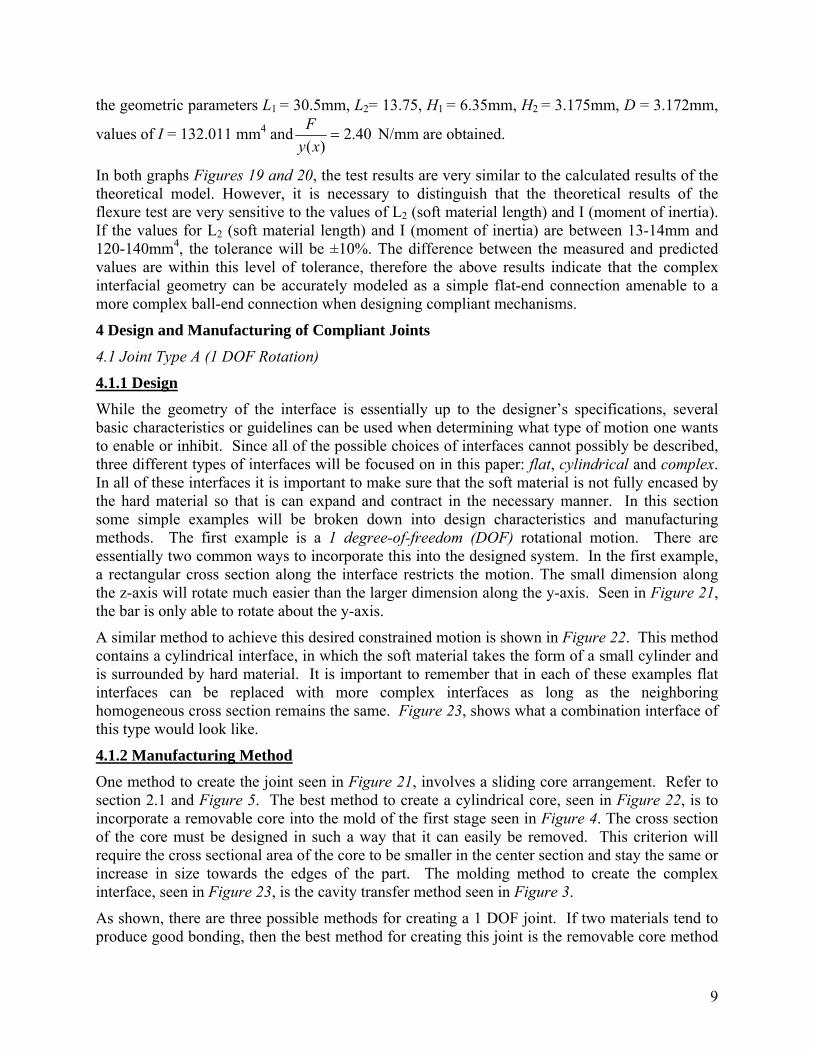
the geometric parameters L1 = 30.5mm, L2= 13.75, H1 = 6.35mm, H2 = 3.175mm, D = 3.172mm,
values of I = 132.011 mm4 and 40.2)(=
xyF N/mm are obtained.
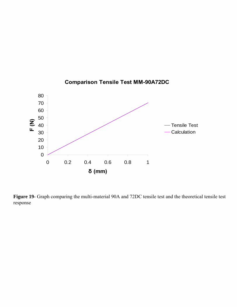
In both graphs Figures 19 and 20, the test results are very similar to the calculated results of the theoretical model. However, it is necessary to distinguish that the theoretical results of the flexure test are very sensitive to the values of L2 (soft material length) and I (moment of inertia). If the values for L2 (soft material length) and I (moment of inertia) are between 13-14mm and 120-140mm4, the tolerance will be ±10%. The difference between the measured and predicted values are within this level of tolerance, therefore the above results indicate that the complex interfacial geometry can be accurately modeled as a simple flat-end connection amenable to a more complex ball-end connection when designing compliant mechanisms.
4 Design and Manufacturing of Compliant Joints
4.1 Joint Type A (1 DOF Rotation)
4.1.1 Design
While the geometry of the interface is essentially up to the designer’s specifications, several basic characteristics or guidelines can be used when determining what type of motion one wants to enable or inhibit. Since all of the possible choices of interfaces cannot possibly be described, three different types of interfaces will be focused on in this paper: flat, cylindrical and complex. In all of these interfaces it is important to make sure that the soft material is not fully encased by the hard material so that is can expand and contract in the necessary manner. In this section some simple examples will be broken down into design characteristics and manufacturing methods. The first example is a 1 degree-of-freedom (DOF) rotational motion. There are essentially two common ways to incorporate this into the designed system. In the first example, a rectangular cross section along the interface restricts the motion. The small dimension along the z-axis will rotate much easier than the larger dimension along the y-axis. Seen in Figure 21, the bar is only able to rotate about the y-axis.
A similar method to achieve this desired constrained motion is shown in Figure 22. This method contains a cylindrical interface, in which the soft material takes the form of a small cylinder and is surrounded by hard material. It is important to remember that in each of these examples flat interfaces can be replaced with more complex interfaces as long as the neighboring homogeneous cross section remains the same. Figure 23, shows what a combination interface of this type would look like.
4.1.2 Manufacturing Method One method to create the joint seen in Figure 21, involves a sliding core arrangement. Refer to section 2.1 and Figure 5. The best method to create a cylindrical core, seen in Figure 22, is to incorporate a removable core into the mold of the first stage seen in Figure 4. The cross section of the core must be designed in such a way that it can easily be removed. This criterion will require the cross sectional area of the core to be smaller in the center section and stay the same or increase in size towards the edges of the part. The molding method to create the complex interface, seen in Figure 23, is the cavity transfer method seen in Figure 3.
As shown, there are three possible methods for creating a 1 DOF joint. If two materials tend to produce good bonding, then the best method for creating this joint is the removable core method
9
which contains the cylindrical core, as seen in Figure 4. This method is preferred because there is very little manipulation between mold stages, therefore, the timing between the mold stages is minimized. The surface area of the joint interface is also maximized promoting more cross linking between the materials. Finally, the cylindrical interface is minimally restrictive on the cross sectional area of the surrounding joint members.
4.2 Joint Type B (2 DOF Rotation)
4.2.1 Design The next example is the design of a joint with 2 DOF rotational motion. In Figure 24, a flat interface with a square cross section can be used to achieve this motion. This geometric configuration allows rotation about the y-axis and z-axis, but is more restrictive in the rotation about a combination of these axes. An alternate method to achieve this movement is shown in Figure 25. A spherical interface is used for this rotational motion. Due to the geometry of the sphere the bar is now free to rotate about the y-axis and z-axis and any combination of these two axes in between. Likewise, a more complex interface can be used to create 2 DOF rotation, shown in Figure 26.
4.2.2 Manufacturing Method The sliding core or removable core manufacturing method, similar to the methods shown in Section 2.1 can be used to create the joint with a flat interface. For a more complex interface, such as the spherical interface (Figure 25), the cavity transfer method must be used. The sphere must be created in the first stage, then manually or robotically transferred into the second mold stage (Figure 27). To create a part similar to Figure 26 the cavity transfer method seen in Figure 3 is used.
For a 2 DOF joint with only rotation about the y and z-axis (not a combination of the axes), the sliding core method is the optimum method to achieve this motion. With this method there is a minimal amount of manipulation between molding stages and the timing between stages can be minimized. However to achieve rotation about a combination of these axes, it would be better to use the cavity transfer method. Although this method requires more manual manipulation, this type of motion causes additional stresses to occur at the interface. Both geometric interlocking as well as chemical bonding are desired to handle this type of loading.
4.3 Joint Type C (3 DOF Rotation)
4.3.1 Design A fourth method to achieve a combination of the y-axis and z-axis with a flat or complex interface would be to use a circular cross sectional area shown in Figure 28. This configuration can also be used to obtain the third DOF: rotation about the x-axis created through the use of twisting or torsional motion. This joint is achieved by a cylindrical interface similar to that of the first example, but is oriented in a different fashion. The circular interface is the least restrictive geometry for the twisting action along the x-axis. In addition it does not introduce many restrictive forces for the rotation about the y and z-axis. There is a general rule in compliant mechanisms: the greater the amount of soft material introduced into the system, the more susceptible the part will be to bending deformations. Therefore, a longer compliant section will tend to bend and twist more easily than a short one. The flat interface in Figure 28, can be replaced by a complex interface shown in Figure 29.
10
4.3.2 Manufacturing Method
In Figure 30, the sliding core method is used to create the flat interface with a circular cross section. The cavity transfer method must be used to create the complex 3 DOF interface. Mold designs for this method are identical to those used for the 1 DOF combination interface, shown in Figure 3.
The 3 DOF joint will have multiple forces acting on it at any given time. It must be able to withstand torsion, tension and flexure loading all at the same time. Due to the nature and probable use of this joint type it is recommended that the joint be configured to promote geometric locking as well as chemical bonding. Therefore, the recommended method for creating this type of joint is the cavity transfer method, using a complex geometry for the interface.
4.4 General Design Guidelines for Compliant Joints
There is a limit to rotational motion along all axis of rotation in compliant joints. For the examples shown, this rotation is limited to 180 degrees of rotation for the y and z-axes, provided the elastic properties of the material are not exceeded causing the part to collide with the base structure. For the twisting rotation about the x-axis this is limited to the elastic properties of the material. However in rotational joints, a small limit in rotation does not always equate to a small amount of movement. The movement attained through rotational motion is directly related to the length of the moment arm, shown in Figure 31. Therefore, a small amount of rotational capabilities can introduce a lot of movement in the structure. This means that rotational compliant joints can be designed to be far more useful than translational compliant joints.
The critical timing characteristics of each stage are largely influenced by the molding method being used to create the part. Minimal manipulation operations, such as removable and sliding core methods, require less hardening time for the first stage. Less hardening time enables the second stage to be poured sooner creating more cross-linking between the two materials at the interface. On the other hand, operations that require large amounts of manipulation between stages, such as the cavity transfer method, require a longer amount of hardening time between molding stages and enable less material adhesion at the interface. This characteristic leads us to a general guideline: if a large amount of manual manipulation is required between molding stages, the interface must be designed to incorporate geometric interlocking at the interface.
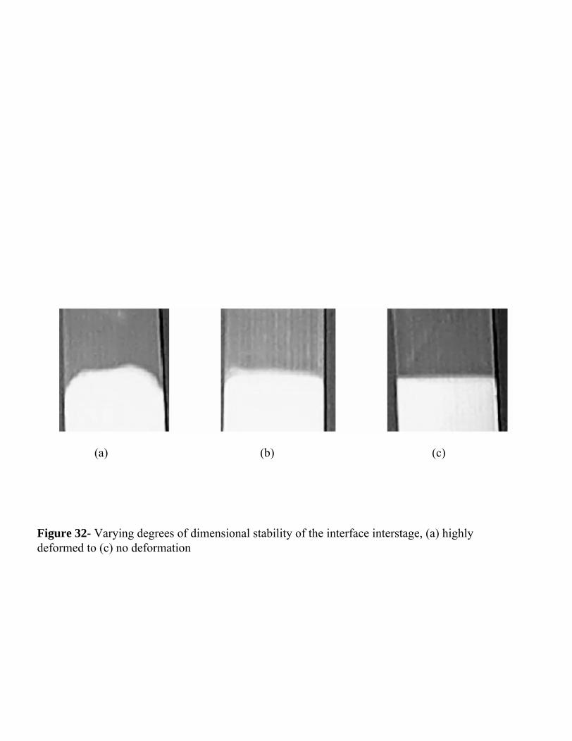
Before deciding on which strategy to use, it is important to experiment with the given materials to determine trade off parameters. These trade off parameters include: (a) measuring the dimensional stability of the interface during the intermediate stage, (b) the overall dimensional stability of the part, and (c) the strength of the interface at the end of each stage. The dimensional stability of the interface at the intermediate stage refers to how malleable and flexible the first stage part will be when it is manipulated into the second molding stage and the second material is shot. If the part is too malleable at this time surface, flaws may occur from both the manipulation and the pressure from the second material. To test this parameter one would have to mold the first stage at different time intervals and measure the deformation of the first stage geometry. Figure 32 shows an example of this deformation after different time intervals. The overall dimensional stability refers to the amount of geometric locking integrated into the interface. To measure the dimensional stability of the part one must mold the part free from chemical bonding.
11
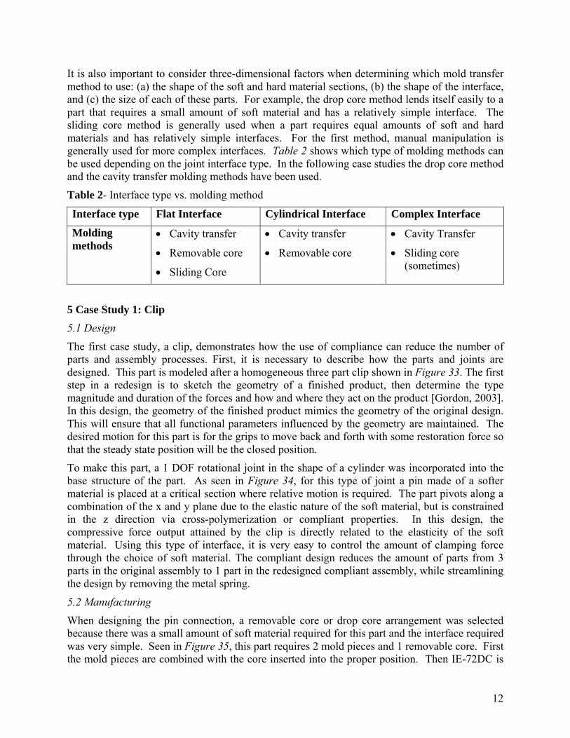
It is also important to consider three-dimensional factors when determining which mold transfer method to use: (a) the shape of the soft and hard material sections, (b) the shape of the interface, and (c) the size of each of these parts. For example, the drop core method lends itself easily to a part that requires a small amount of soft material and has a relatively simple interface. The sliding core method is generally used when a part requires equal amounts of soft and hard materials and has relatively simple interfaces. For the first method, manual manipulation is generally used for more complex interfaces. Table 2 shows which type of molding methods can be used depending on the joint interface type. In the following case studies the drop core method and the cavity transfer molding methods have been used.
Table 2- Interface type vs. molding method
Interface type Flat Interface Cylindrical Interface Complex Interface
Molding methods
• Cavity transfer
• Removable core
• Sliding Core
• Cavity transfer
• Removable core
• Cavity Transfer
• Sliding core (sometimes)
5 Case Study 1: Clip
5.1 Design
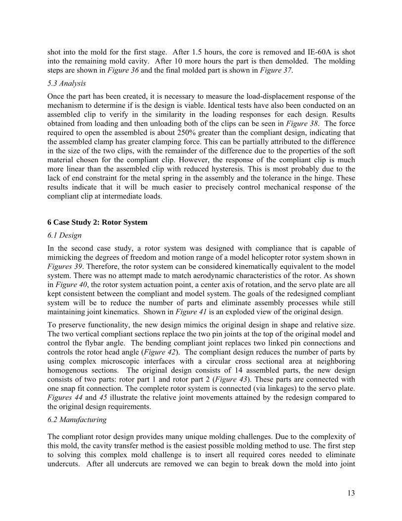
The first case study, a clip, demonstrates how the use of compliance can reduce the number of parts and assembly processes. First, it is necessary to describe how the parts and joints are designed. This part is modeled after a homogeneous three part clip shown in Figure 33. The first step in a redesign is to sketch the geometry of a finished product, then determine the type magnitude and duration of the forces and how and where they act on the product [Gordon, 2003]. In this design, the geometry of the finished product mimics the geometry of the original design. This will ensure that all functional parameters influenced by the geometry are maintained. The desired motion for this part is for the grips to move back and forth with some restoration force so that the steady state position will be the closed position.
To make this part, a 1 DOF rotational joint in the shape of a cylinder was incorporated into the base structure of the part. As seen in Figure 34, for this type of joint a pin made of a softer material is placed at a critical section where relative motion is required. The part pivots along a combination of the x and y plane due to the elastic nature of the soft material, but is constrained in the z direction via cross-polymerization or compliant properties. In this design, the compressive force output attained by the clip is directly related to the elasticity of the soft material. Using this type of interface, it is very easy to control the amount of clamping force through the choice of soft material. The compliant design reduces the amount of parts from 3 parts in the original assembly to 1 part in the redesigned compliant assembly, while streamlining the design by removing the metal spring.
5.2 Manufacturing
When designing the pin connection, a removable core or drop core arrangement was selected because there was a small amount of soft material required for this part and the interface required was very simple. Seen in Figure 35, this part requires 2 mold pieces and 1 removable core. First the mold pieces are combined with the core inserted into the proper position. Then IE-72DC is
12
shot into the mold for the first stage. After 1.5 hours, the core is removed and IE-60A is shot into the remaining mold cavity. After 10 more hours the part is then demolded. The molding steps are shown in Figure 36 and the final molded part is shown in Figure 37.
5.3 Analysis
Once the part has been created, it is necessary to measure the load-displacement response of the mechanism to determine if is the design is viable. Identical tests have also been conducted on an assembled clip to verify in the similarity in the loading responses for each design. Results obtained from loading and then unloading both of the clips can be seen in Figure 38. The force required to open the assembled is about 250% greater than the compliant design, indicating that the assembled clamp has greater clamping force. This can be partially attributed to the difference in the size of the two clips, with the remainder of the difference due to the properties of the soft material chosen for the compliant clip. However, the response of the compliant clip is much more linear than the assembled clip with reduced hysteresis. This is most probably due to the lack of end constraint for the metal spring in the assembly and the tolerance in the hinge. These results indicate that it will be much easier to precisely control mechanical response of the compliant clip at intermediate loads.
6 Case Study 2: Rotor System
6.1 Design
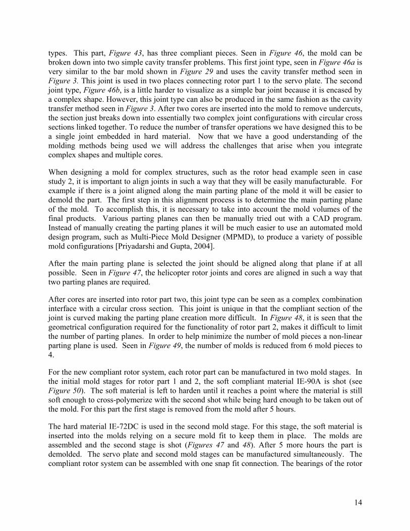
In the second case study, a rotor system was designed with compliance that is capable of mimicking the degrees of freedom and motion range of a model helicopter rotor system shown in Figures 39. Therefore, the rotor system can be considered kinematically equivalent to the model system. There was no attempt made to match aerodynamic characteristics of the rotor. As shown in Figure 40, the rotor system actuation point, a center axis of rotation, and the servo plate are all kept consistent between the compliant and model system. The goals of the redesigned compliant system will be to reduce the number of parts and eliminate assembly processes while still maintaining joint kinematics. Shown in Figure 41 is an exploded view of the original design.
To preserve functionality, the new design mimics the original design in shape and relative size. The two vertical compliant sections replace the two pin joints at the top of the original model and control the flybar angle. The bending compliant joint replaces two linked pin connections and controls the rotor head angle (Figure 42). The compliant design reduces the number of parts by using complex microscopic interfaces with a circular cross sectional area at neighboring homogenous sections. The original design consists of 14 assembled parts, the new design consists of two parts: rotor part 1 and rotor part 2 (Figure 43). These parts are connected with one snap fit connection. The complete rotor system is connected (via linkages) to the servo plate. Figures 44 and 45 illustrate the relative joint movements attained by the redesign compared to the original design requirements.
6.2 Manufacturing
The compliant rotor design provides many unique molding challenges. Due to the complexity of this mold, the cavity transfer method is the easiest possible molding method to use. The first step to solving this complex mold challenge is to insert all required cores needed to eliminate undercuts. After all undercuts are removed we can begin to break down the mold into joint
13
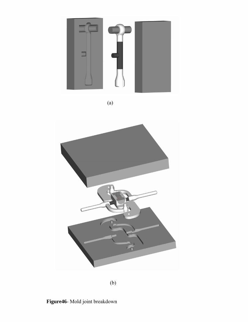
types. This part, Figure 43, has three compliant pieces. Seen in Figure 46, the mold can be broken down into two simple cavity transfer problems. This first joint type, seen in Figure 46a is very similar to the bar mold shown in Figure 29 and uses the cavity transfer method seen in Figure 3. This joint is used in two places connecting rotor part 1 to the servo plate. The second joint type, Figure 46b, is a little harder to visualize as a simple bar joint because it is encased by a complex shape. However, this joint type can also be produced in the same fashion as the cavity transfer method seen in Figure 3. After two cores are inserted into the mold to remove undercuts, the section just breaks down into essentially two complex joint configurations with circular cross sections linked together. To reduce the number of transfer operations we have designed this to be a single joint embedded in hard material. Now that we have a good understanding of the molding methods being used we will address the challenges that arise when you integrate complex shapes and multiple cores.
When designing a mold for complex structures, such as the rotor head example seen in case study 2, it is important to align joints in such a way that they will be easily manufacturable. For example if there is a joint aligned along the main parting plane of the mold it will be easier to demold the part. The first step in this alignment process is to determine the main parting plane of the mold. To accomplish this, it is necessary to take into account the mold volumes of the final products. Various parting planes can then be manually tried out with a CAD program. Instead of manually creating the parting planes it will be much easier to use an automated mold design program, such as Multi-Piece Mold Designer (MPMD), to produce a variety of possible mold configurations [Priyadarshi and Gupta, 2004].
After the main parting plane is selected the joint should be aligned along that plane if at all possible. Seen in Figure 47, the helicopter rotor joints and cores are aligned in such a way that two parting planes are required.
After cores are inserted into rotor part two, this joint type can be seen as a complex combination interface with a circular cross section. This joint is unique in that the compliant section of the joint is curved making the parting plane creation more difficult. In Figure 48, it is seen that the geometrical configuration required for the functionality of rotor part 2, makes it difficult to limit the number of parting planes. In order to help minimize the number of mold pieces a non-linear parting plane is used. Seen in Figure 49, the number of molds is reduced from 6 mold pieces to 4.
For the new compliant rotor system, each rotor part can be manufactured in two mold stages. In the initial mold stages for rotor part 1 and 2, the soft compliant material IE-90A is shot (see Figure 50). The soft material is left to harden until it reaches a point where the material is still soft enough to cross-polymerize with the second shot while being hard enough to be taken out of the mold. For this part the first stage is removed from the mold after 5 hours.
The hard material IE-72DC is used in the second mold stage. For this stage, the soft material is inserted into the molds relying on a secure mold fit to keep them in place. The molds are assembled and the second stage is shot (Figures 47 and 48). After 5 more hours the part is demolded. The servo plate and second mold stages can be manufactured simultaneously. The compliant rotor system can be assembled with one snap fit connection. The bearings of the rotor
14
part 2 snap in the rotor part 1. The complete compliant rotor system is connected with the servo plate via linkages (Figure 51).
6.3 Analysis
This example was quite complex and creating force vs. displacement required development of custom test fixtures. So in this case we analyzed the mechanism using finite element-based analysis tool Pro/Mechanica.
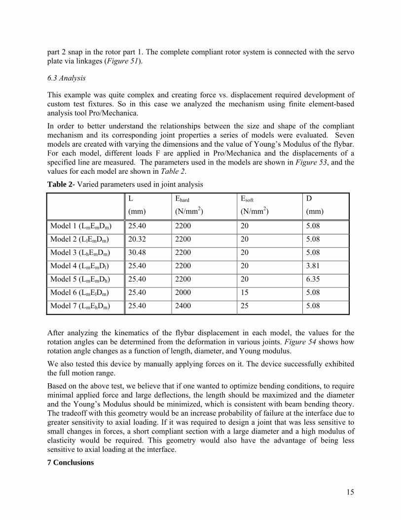
In order to better understand the relationships between the size and shape of the compliant mechanism and its corresponding joint properties a series of models were evaluated. Seven models are created with varying the dimensions and the value of Young’s Modulus of the flybar. For each model, different loads F are applied in Pro/Mechanica and the displacements of a specified line are measured. The parameters used in the models are shown in Figure 53, and the values for each model are shown in Table 2.
Table 2- Varied parameters used in joint analysis
L
(mm)
Ehard
(N/mm2)
Esoft
(N/mm2)
D
(mm)
Model 1 (LmEmDm) 25.40 2200 20 5.08
Model 2 (LlEmDm) 20.32 2200 20 5.08
Model 3 (LhEmDm) 30.48 2200 20 5.08
Model 4 (LmEmDl) 25.40 2200 20 3.81
Model 5 (LmEmDh) 25.40 2200 20 6.35
Model 6 (LmElDm) 25.40 2000 15 5.08
Model 7 (LmEhDm) 25.40 2400 25 5.08
After analyzing the kinematics of the flybar displacement in each model, the values for the rotation angles can be determined from the deformation in various joints. Figure 54 shows how rotation angle changes as a function of length, diameter, and Young modulus.
We also tested this device by manually applying forces on it. The device successfully exhibited the full motion range.
Based on the above test, we believe that if one wanted to optimize bending conditions, to require minimal applied force and large deflections, the length should be maximized and the diameter and the Young’s Modulus should be minimized, which is consistent with beam bending theory. The tradeoff with this geometry would be an increase probability of failure at the interface due to greater sensitivity to axial loading. If it was required to design a joint that was less sensitive to small changes in forces, a short compliant section with a large diameter and a high modulus of elasticity would be required. This geometry would also have the advantage of being less sensitive to axial loading at the interface.
7 Conclusions
15
This paper shows that multi-material molding is a promising manufacturing process for creating multi-material compliant mechanisms. Several different types of interfaces that can be used in compliant mechanisms are described. Experimental characterization results for these interfaces show that these interfaces have the required motion range and do not break under the loads needed to produce the motion. Furthermore, experimental characterization results show that certain geometrically complex interfaces can be modeled as simple interfaces without having any serious affect on the accuracy of an assembly analysis. This paper also describes design of several different compliant joints that provide one to three degrees of freedom. For each joint design, we also present a feasible mold design to realize that joint. Finally, we show how a complex device consisting multiple different compliant joints can be fabricated by combining mold pieces for individual joints into an overall mold.
The case studies clearly show that compliant joints can be used to reduce part count and eliminate assembly operations. In the clip assembly the part count is reduced by 66.6% and in the rotor assembly the part count is reduced by 85.7%. Along with these manufacturing benefits, multi-material compliant mechanisms can be used to create geometrically complex structures, seen in the rotor example. While there are several different methods to create multi-material compliant mechanisms, the multi-material molding method it superior because of it’s adaptability to traditional molding technologies. This adaptability enables one to create very complex structures at highly reduced costs.
In large batch production, the cost of molds is amortized over a large number of parts. Hence, the molding process exhibits economy of scale. Unfortunately, layered fabrication processes do not exhibit economy of scale. Therefore, for multi-material structures that are manufacturable using molding, the processing cost is significantly lower compared to the layered processes for making these structures (e.g., 3D printing) when the batch size is large. Therefore, multi-material molding (MMM) is becoming increasingly popular in the manufacturing industry due to its ability to produce higher-quality multi-material products.
It is important to understand that each MMM process has its own advantages, disadvantages and limitations in addition to added costs associated with equipment. It is important to choose the right process and material combinations for a given application in order to maximize product quality and profit. The design and manufacturing approach described in this paper is the first step towards development of an integrated product/process development methodology for molded MM structures.
Acknowledgements. This research has been supported in part by NSF grants DMI0093142 and EEC0315425, and Army Research Office through MAV MURI Program (Grant No. ARMY-W911NF0410176). Opinions expressed in this paper are those of authors and do not necessarily reflect opinion of the sponsors.
8 References [Ananthasuresh and Kota, 1995] G.K. Ananthasuresh and S. Kota. Designing Compliant Mechanisms. Mechanical Engineering, 117(11):93-96, 1995.
16
[Bailey et al., 1999] S.A. Bailey, J.G. Cham, M.R. Cutkosky, and R.J. Full. Biomimetic Robotic Mechanisms via Shape Deposition Manufacturing. 9th International Symposium of Robotics Research, Utah, October 1999.
[Beaman et al., 2000] J. Beaman, D. Bourell, B. Jackson, L. Jepson, D. McAdams, J. Perez, and K. Wood. Multi-Material Selective Laser Sintering: Empirical Studies and Hardware Development. NSF Design and Manufacturing Grantees Conference, January 2000.
[Bruck et al., 2004] H.A. Bruck, G. Fowler, S.K. Gupta, and T.M. Valentine. Using Geometric Complexity to Enhance the Interfacial Strength of Heterogeneous Structures Fabricated in a Multi-Stage, Multi-Piece Molding Process. Experimental Mechanics, 44:261-271, 2004.
[Bryce, 1996] D.M. Bryce. Plastic Injection Molding, Vol. I: Manufacturing Process Fundamentals. Society of Manufacturing Engineers: Dearborn, Michigan, 1996.
[Goldin et al., 2000] D.S. Goldin, S.L. Venneri, and A.K. Noor. The great out of the small. Mechanical Engineering, 122:70-79, 2000.
[Gordon, 2003] M.J. Gordon, Jr. Industrial Design of Plastic Products. John Wiley & Sons, Inc.: Hoboken, New Jersey, 2003.
[Goodship and Love, 2002] V. Goodship and J.C. Love. Multi-Material Injection Moulding. Rapra Technology LTD.: Shawbury, UK, 2002.
[Howell, 2001] L.L. Howell. Compliant Mechanisms. John Wiley and Sons: New York, New York, 2001.
[Howell et al., 1996] L.L Howell, A. Midha, and T. W. Norton. Evaluation of Equivalent Spring Stiffness for Use in a Pseudo-Rigid-Body Model of Large-Deflection Compliant Mechanisms. ASME Journal of Mechanical Design, 118:125-131, 1996.
[Jackson et al., 1998] T.P. Jackson, E.M. Sachs, and M.J. Cima. Modeling and Designing Components with Locally Controlled Composition. Solid Freeform Fabrication Symposium, August 1998.
[Kumar, 2001] M. Kumar. Automated Design of Multi-Stage Molds For Manufacturing Multi-Material Objects. M.S. Thesis, University of Maryland, College Park, MD, 2001.
[Malloy, 1994] R.A. Malloy. Plastic Part Design for Injection Molding: And Introduction. Hanser Gardner Publications, Inc.: Cincinnati, Ohio, 1994.
[Maniscalco, 2004] M. Maniscalco. Basic Elements: Simplifying multicomponent design. IMM Magazine (online version). 3/2004. http://www.immnet.com/articles?article=2343.
[Pirkl, 1998] J.D. Pirkl. Automating the Multi-Component Molding Process. In Proceedings of Technologies for Multi-Material Injection Molding (CM98-206), Troy, Michigan, May 1998.
17
[Plank, 2002] H. Plank. Overmolding-Stack-Mold Technology: An Innovative Concept in Multi-Component Injection Molding. SME Technical Papers (CM02-225), 2002.
[Priyadarshi and Gupta, 2004] A. Priyadarshi, and S.K. Gupta. Geometric algorithms for automated design of multi-piece permanent molds. Computer Aided Design, 36(3):241-260, 2004.
[Rotheiser, 2004] J. Rotheiser. Joining of Plastics, Handbook for Designers and Engineers. Hanser Gardner Publications, Inc.: Cincinnati, Ohio, 2004.
[van Krevelen, 1990] D.W. van Krevelen. Properties of Polymers. Elsevier: New York, New York, 1990.
[Vogel, 1995] S. Vogel. Better Bent Than Broken. Discover, 16(5), 1995.
18
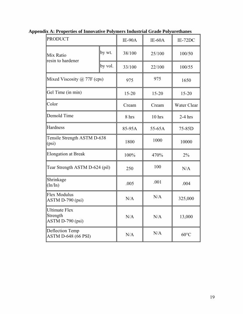
Appendix A: Properties of Innovative Polymers Industrial Grade Polyurethanes PRODUCT IE-90A IE-60A IE-72DC
by wt.
38/100 25/100 100/50 Mix Ratio resin to hardener
by vol. 33/100 22/100 100/55
Mixed Viscosity @ 77F (cps) 975 975 1650
Gel Time (in min) 15-20 15-20 15-20
Color Cream Cream Water Clear
Demold Time 8 hrs 10 hrs 2-4 hrs
Hardness 85-95A 55-65A 75-85D
Tensile Strength ASTM D-638 (psi) 1800 1000 10000
Elongation at Break 100% 470% 2%
Tear Strength ASTM D-624 (pil) 250 100 N/A
Shrinkage (In/In) .005 .001 .004
Flex Modulus ASTM D-790 (psi) N/A N/A 325,000
Ultimate Flex Strength ASTM D-790 (psi)
N/A
N/A 13,000
Deflection Temp ASTM D-648 (66 PSI) N/A N/A 60°C
19
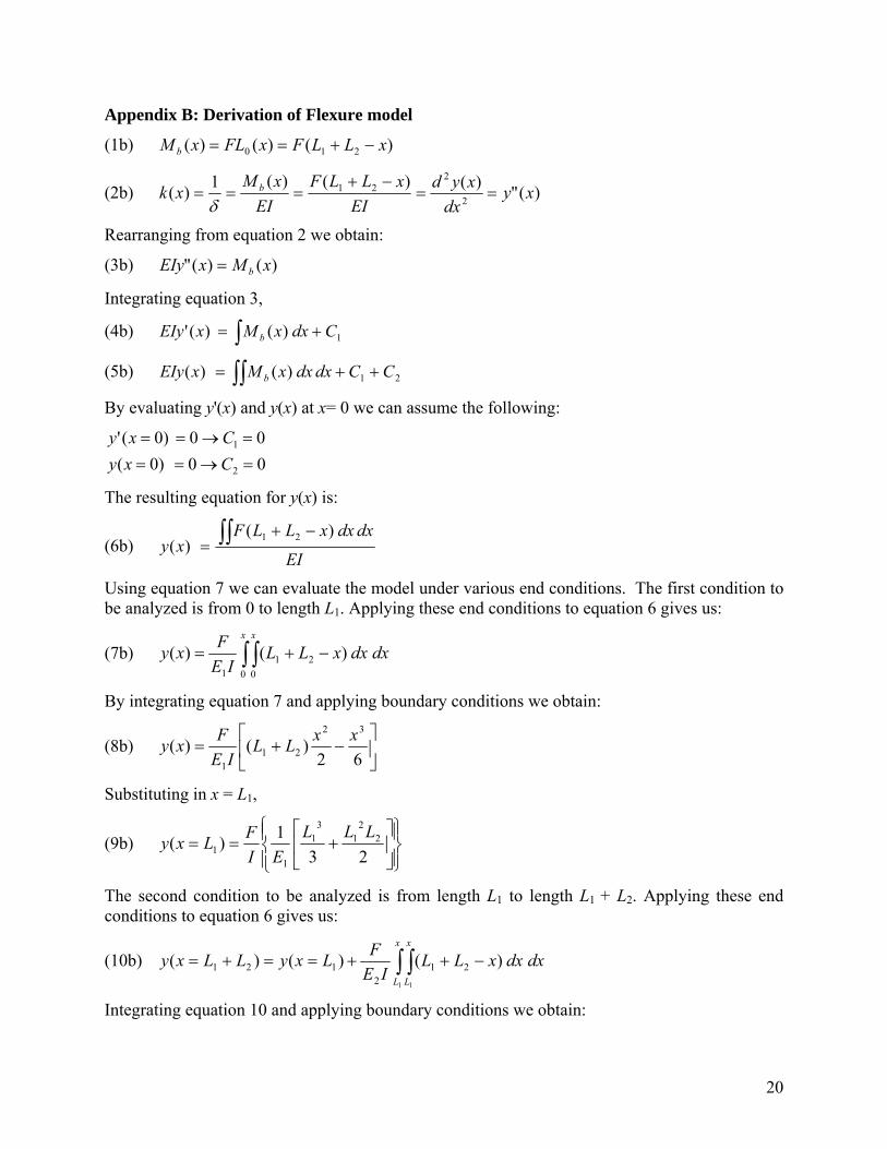
Appendix B: Derivation of Flexure model
(1b) )()()( 210 xLLFxFLxM b −+==
(2b) )(")()()(1)( 2
221 xy
dxxyd
EIxLLF
EIxM
xk b ==−+
===δ
Rearranging from equation 2 we obtain:
(3b) )()(" xMxEIy b=
Integrating equation 3,
(4b) 1)()(' CdxxMxEIy b += ∫(5b) 21)()( CCdxdxxMxEIy b ++= ∫∫By evaluating y'(x) and y(x) at x= 0 we can assume the following:
00)0(00)0('
2
1
=→===→==
CxyCxy
The resulting equation for y(x) is:
(6b) EI
dxdxxLLFxy ∫∫ −+
=)(
)(21
Using equation 7 we can evaluate the model under various end conditions. The first condition to be analyzed is from 0 to length L1. Applying these end conditions to equation 6 gives us:
(7b) dxdxxLLIE
Fxyx x
∫ ∫ −+=0 0
211
)()(
By integrating equation 7 and applying boundary conditions we obtain:
(8b) ⎥⎦
⎤⎢⎣
⎡−+=
62)()(
32
211
xxLLIE
Fxy
Substituting in x = L1,
(9b) ⎪⎩
⎪⎨⎧
⎪⎭
⎪⎬⎫⎥⎦
⎤⎢⎣
⎡+==
231)( 2
21
31
11
LLLEI
FLxy
The second condition to be analyzed is from length L1 to length L1 + L2. Applying these end conditions to equation 6 gives us:
(10b) dxdxxLLIE
FLxyLLxyx
L
x
L∫ ∫ −++==+=
1 1
)()()( 212
121
Integrating equation 10 and applying boundary conditions we obtain:
20
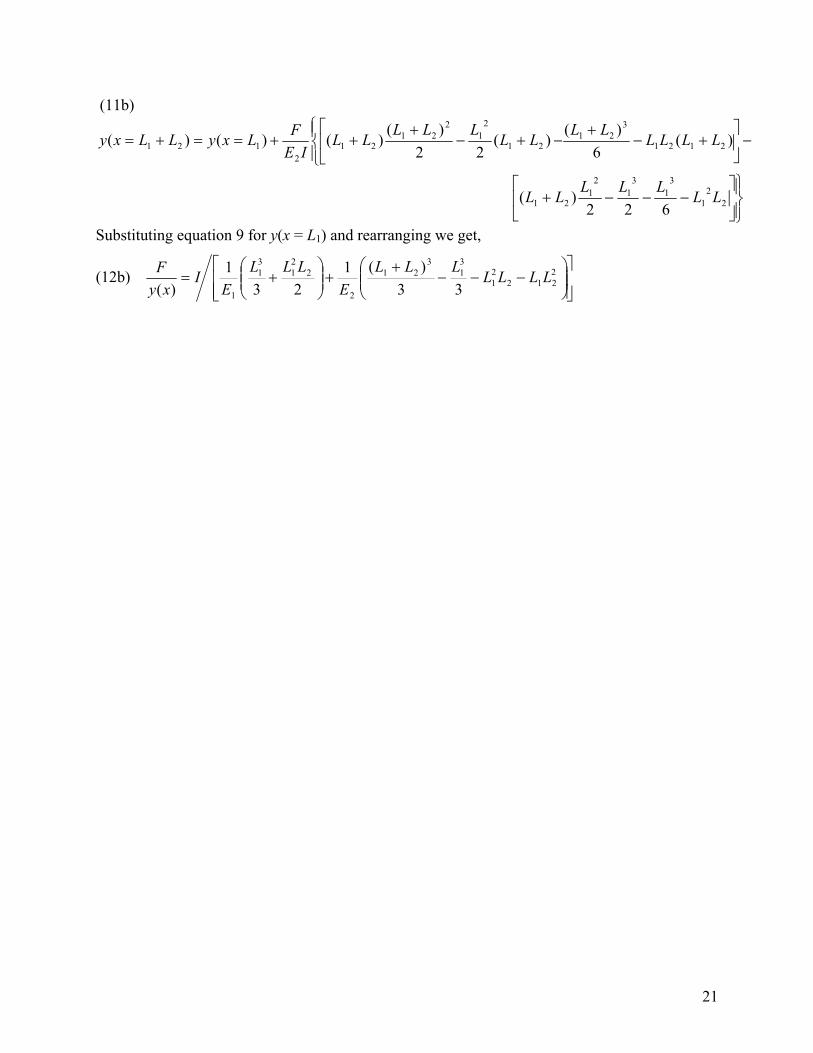
(11b)
⎪⎭
⎪⎬⎫⎥⎦
⎤⎢⎣
⎡−−−+
−⎥⎦
⎤+−
+
⎪⎩
⎪⎨⎧⎢⎣
⎡−+−
+++==+=
22
1
31
31
21
21
2121
321
21
21
221
212
121
622)(
)(6
)()(22
)()()()(
LLLLLLL
LLLLLLLLLLLLLIE
FLxyLLxy
Substituting equation 9 for y(x = L1) and rearranging we get,
(12b) ⎥⎥⎦
⎤
⎢⎢⎣
⎡⎟⎟⎠
⎞⎜⎜⎝
⎛−−−
++⎟⎟
⎠
⎞⎜⎜⎝
⎛+= 2
21221
31
321
2
221
31
1 33)(1
231
)(LLLL
LLLE
LLLE
Ixy
F
21
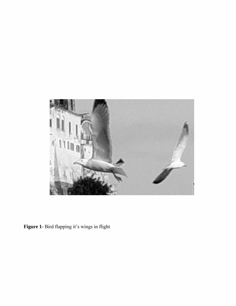
Figure 1- Bird flapping it’s wings in flight
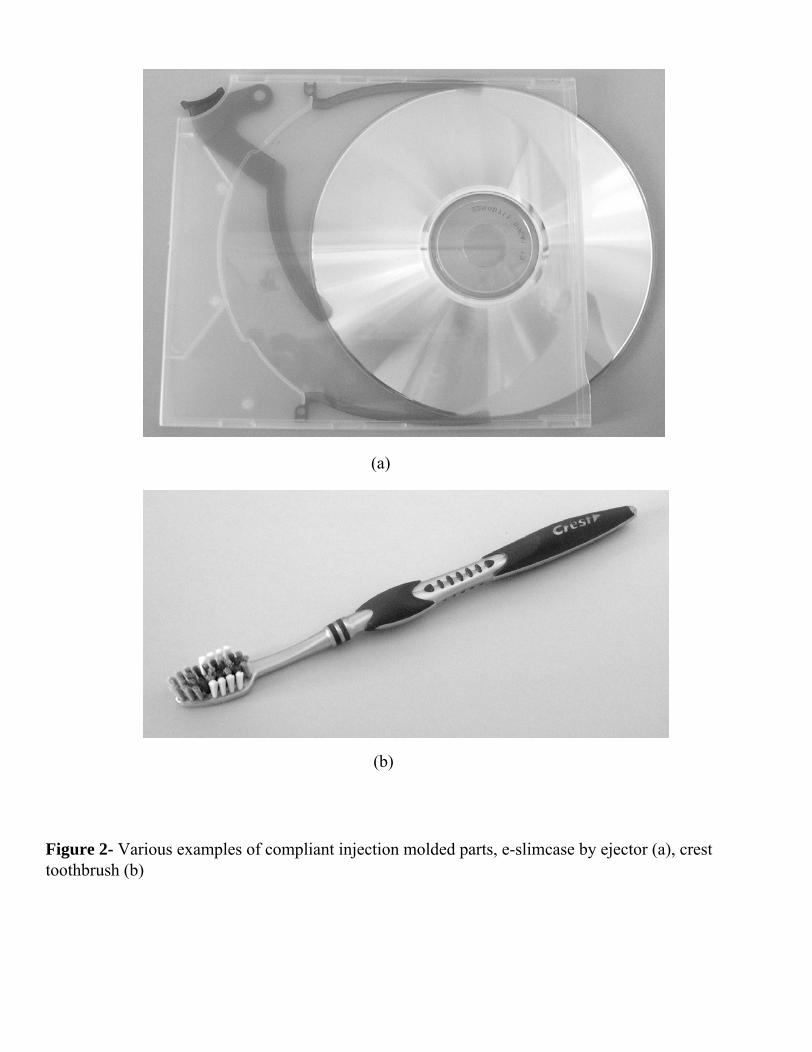
Figure 2- Various examples of compliant injection molded parts, e-slimcase by ejector (a), crest toothbrush (b)
(a)
(b)
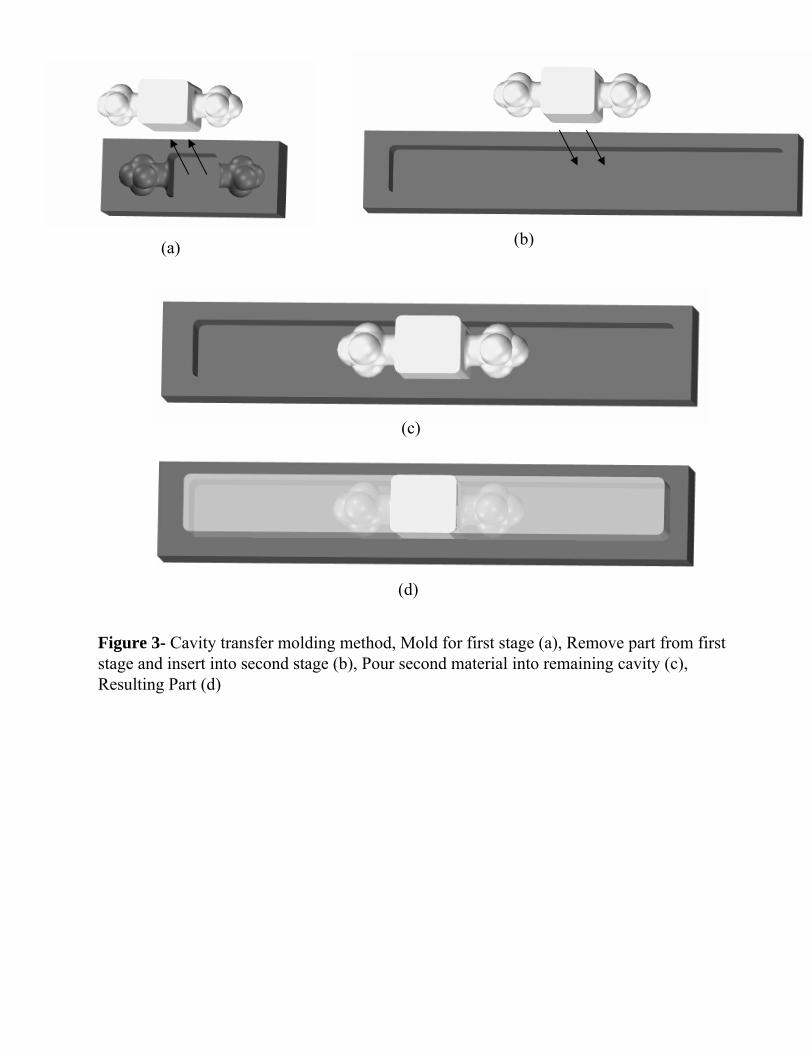
Figure 3- Cavity transfer molding method, Mold for first stage (a), Remove part from first stage and insert into second stage (b), Pour second material into remaining cavity (c), Resulting Part (d)
(a) (b)
(c)
(d)
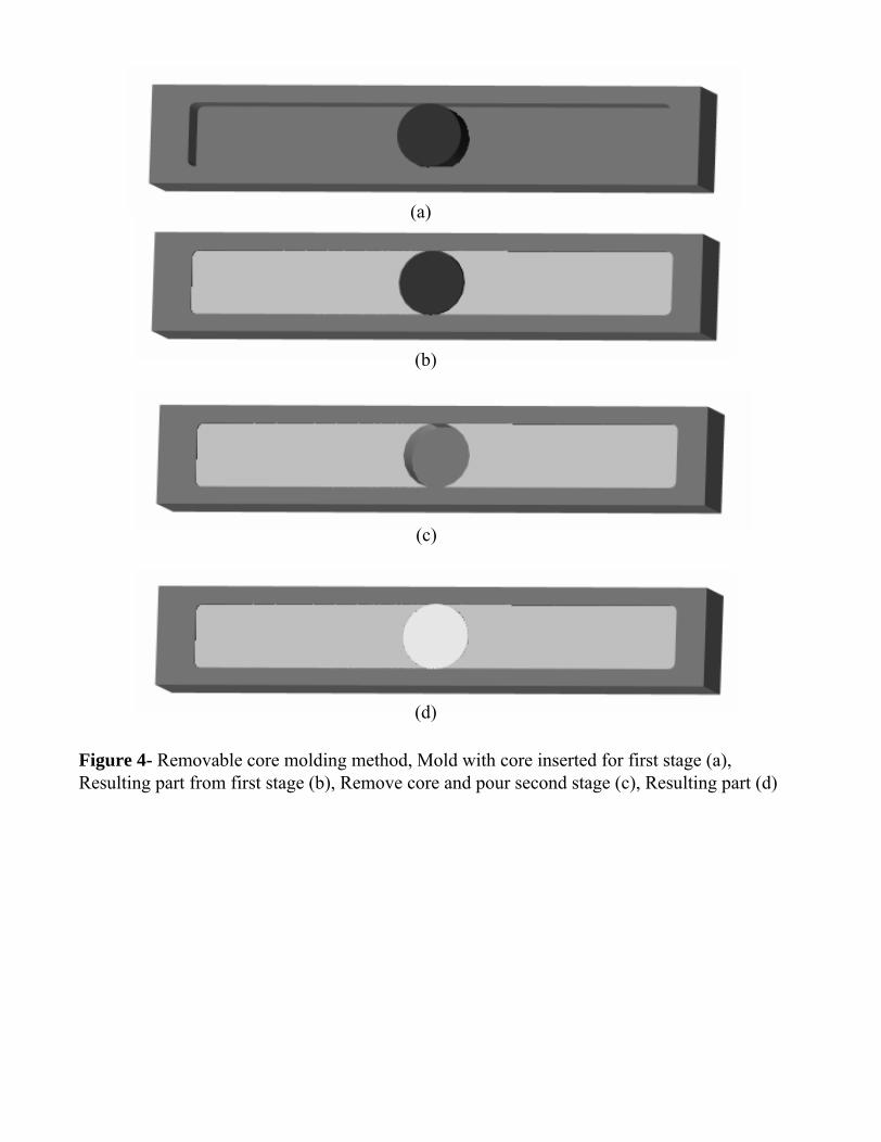
Figure 4- Removable core molding method, Mold with core inserted for first stage (a), Resulting part from first stage (b), Remove core and pour second stage (c), Resulting part (d)
(a)
(b)
(c)
(d)
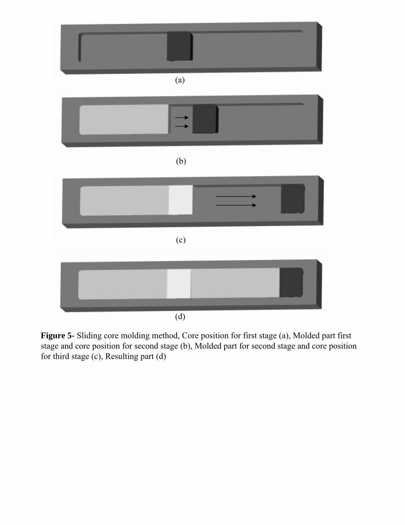
Figure 5- Sliding core molding method, Core position for first stage (a), Molded part first stage and core position for second stage (b), Molded part for second stage and core position for third stage (c), Resulting part (d)
(a)
(b)
(c)
(d)
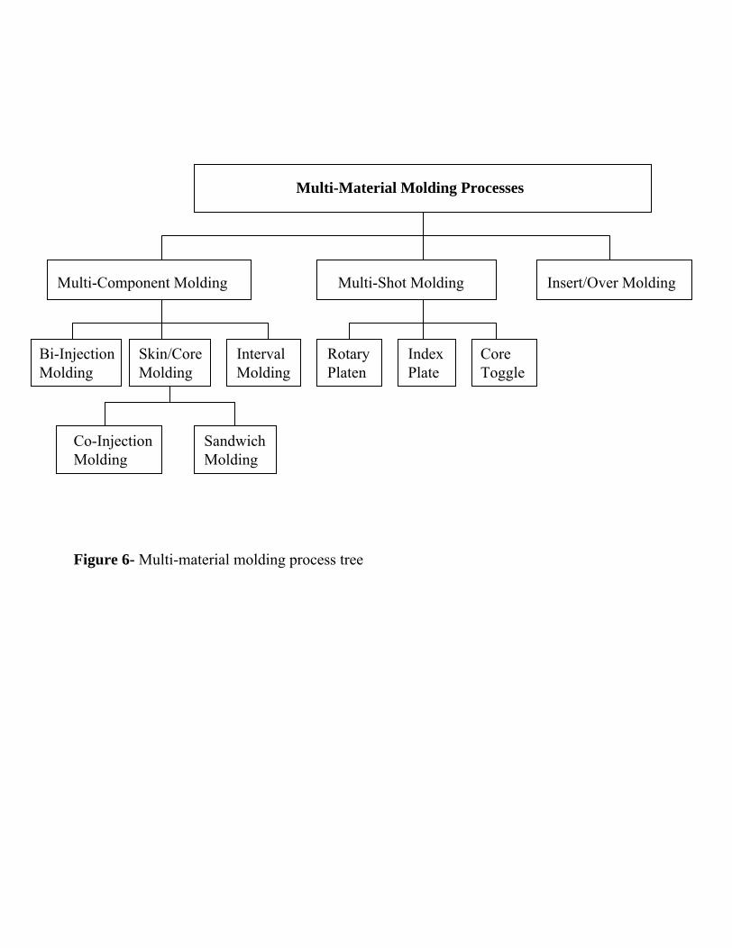
Figure 6- Multi-material molding process tree
Multi-Material Molding Processes
Multi-Component Molding Multi-Shot Molding Insert/Over Molding
Bi-InjectionMolding
Skin/CoreMolding
IntervalMolding
RotaryPlaten
IndexPlate
CoreToggle
Co-InjectionMolding
SandwichMolding
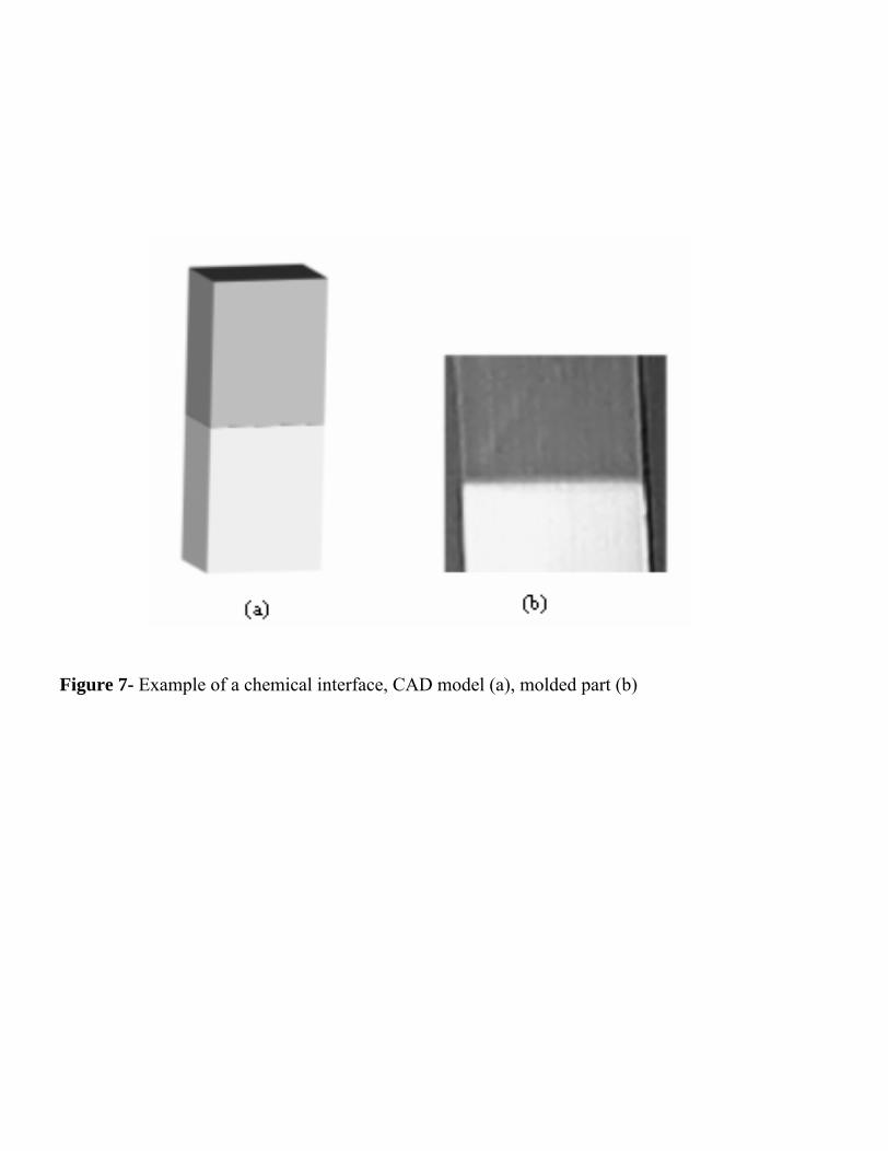
Figure 7- Example of a chemical interface, CAD model (a), molded part (b)
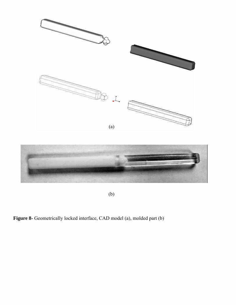
Figure 8- Geometrically locked interface, CAD model (a), molded part (b)
(a)
(b)
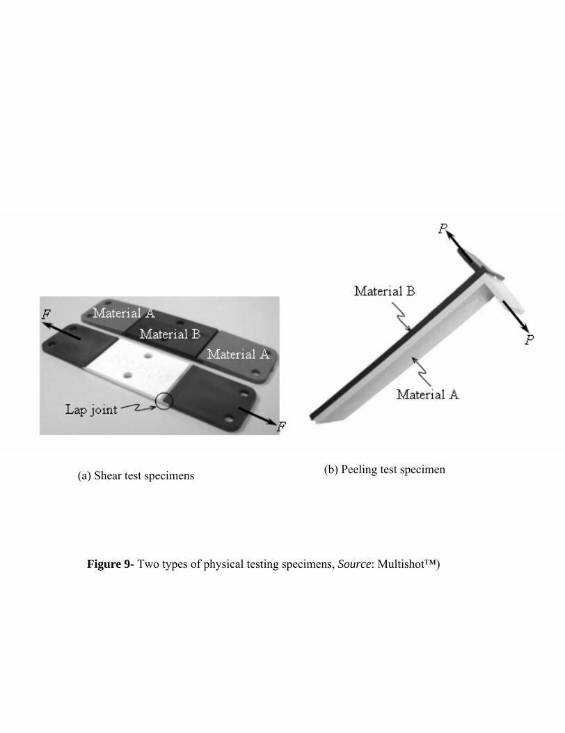
Figure 9- Two types of physical testing specimens, Source: Multishot™)
(b) Peeling test specimen(a) Shear test specimens
(a) – before failure (b) – after failure
Figure 10- Tensile test specimen geometry
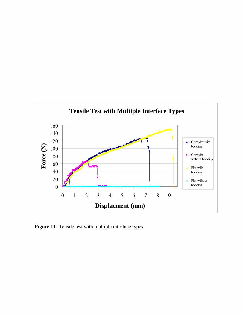
Figure 11- Tensile test with multiple interface types
Tensile Test with Multiple Interface Types
020406080
100120140160
0 1 2 3 4 5 6 7 8 9
Displacment (mm)
Forc
e (N
) Complex withbonding
Complexwithout bonding
Flat withbonding
Flat withoutbonding
E1
E2
L0
L2
L1
δ
A
F
F
Figure 12- Schematic diagram of the tensile test variables
σ = stressE = young’s modulusE1 = young’s modulus material 1E2 = young’s modulus material 2 ε = strainF = force or loadA = cross-sectional areaδ = extension lengthL0 = original complete lengthL1 = original length material 1L2 = original length material 2
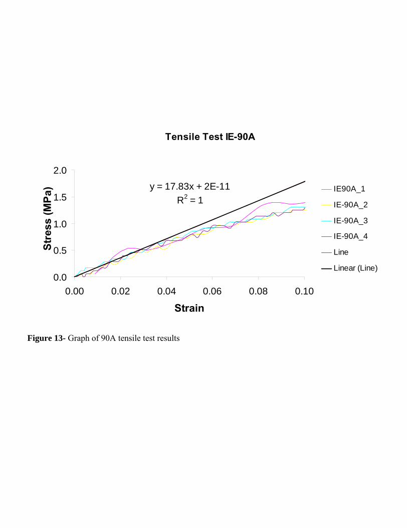
Figure 13- Graph of 90A tensile test results
Tensile Test IE-90A
y = 17.83x + 2E-11R2 = 1
0.0
0.5
1.0
1.5
2.0
0.00 0.02 0.04 0.06 0.08 0.10
Strain
Stre
ss (M
Pa) IE90A_1
IE-90A_2
IE-90A_3
IE-90A_4
Line
Linear (Line)

Tensile Test IE-72DC
y = 2493.4x + 2E-14R2 = 1
01020304050607080
0.00 0.01 0.02 0.03 0.04
Strain
Stre
ss (M
Pa)
IE-72DC_6IE-72DC_7IE-72DC_8IE-72DC_9IE-72DC_10LineLinear (Line)
Figure 14- Graph of 72DC tensile test results
Tensile Test MM-90A72DC
y = 70.203x - 1E-07R2 = 1
01020
30405060
7080
0 0.2 0.4 0.6 0.8 1
δ (mm)
F (N
) MM-90A72DC_3MM-90A72DC_4LineLinear (Line)
Figure 15- Graph of multi-material 90A and 72DC tensile test results
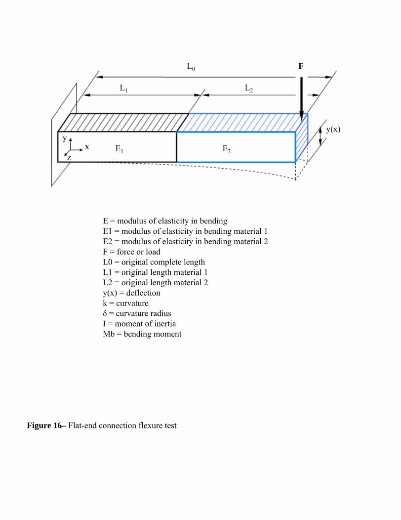
E = modulus of elasticity in bendingE1 = modulus of elasticity in bending material 1E2 = modulus of elasticity in bending material 2 F = force or loadL0 = original complete lengthL1 = original length material 1L2 = original length material 2y(x) = deflectionk = curvatureδ = curvature radiusI = moment of inertia Mb = bending moment
Figure 16– Flat-end connection flexure test
L0
L1 L2
F
E1 E2x
y
z
y(x)
Flexure Test MM-90A72DC
y = 2.7072x + 9E-07R2 = 1
012345678
0 1 2
y (x,mm)
F (N
)
MM-90A72DC_5
MM-90A72DC_6
Line
Linear (Line)
Figure 17- Graph of multi-material 90A and 72DC flexure test results
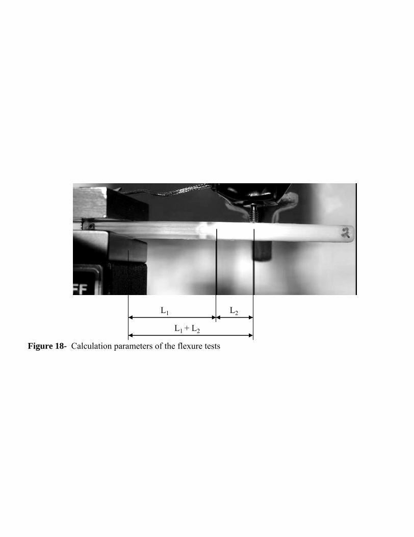
Figure 18- Calculation parameters of the flexure tests
L1 L2
L1 + L2
Comparison Tensile Test MM-90A72DC
01020304050607080
0 0.2 0.4 0.6 0.8 1
δ (mm)
F (N
)
Tensile TestCalculation
Figure 19- Graph comparing the multi-material 90A and 72DC tensile test and the theoretical tensile test response
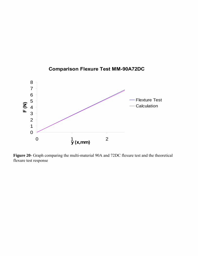
Comparison Flexure Test MM-90A72DC
012345678
0 1 2y (x,mm)
F (N
) Flexture TestCalculation
Figure 20- Graph comparing the multi-material 90A and 72DC flexure test and the theoretical flexure test response
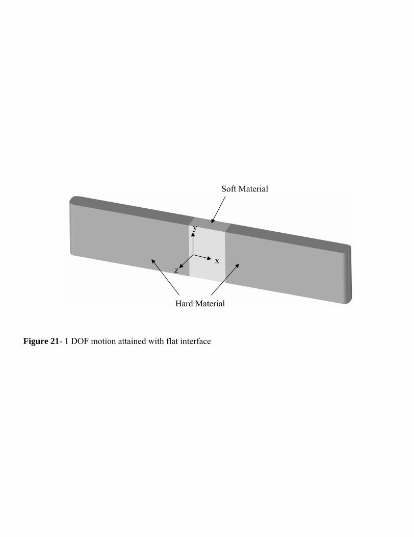
Figure 21- 1 DOF motion attained with flat interface
Hard Material
Soft Material
x
y
z
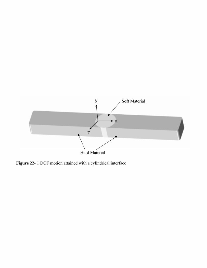
Figure 22- 1 DOF motion attained with a cylindrical interface
Soft Material
Hard Material
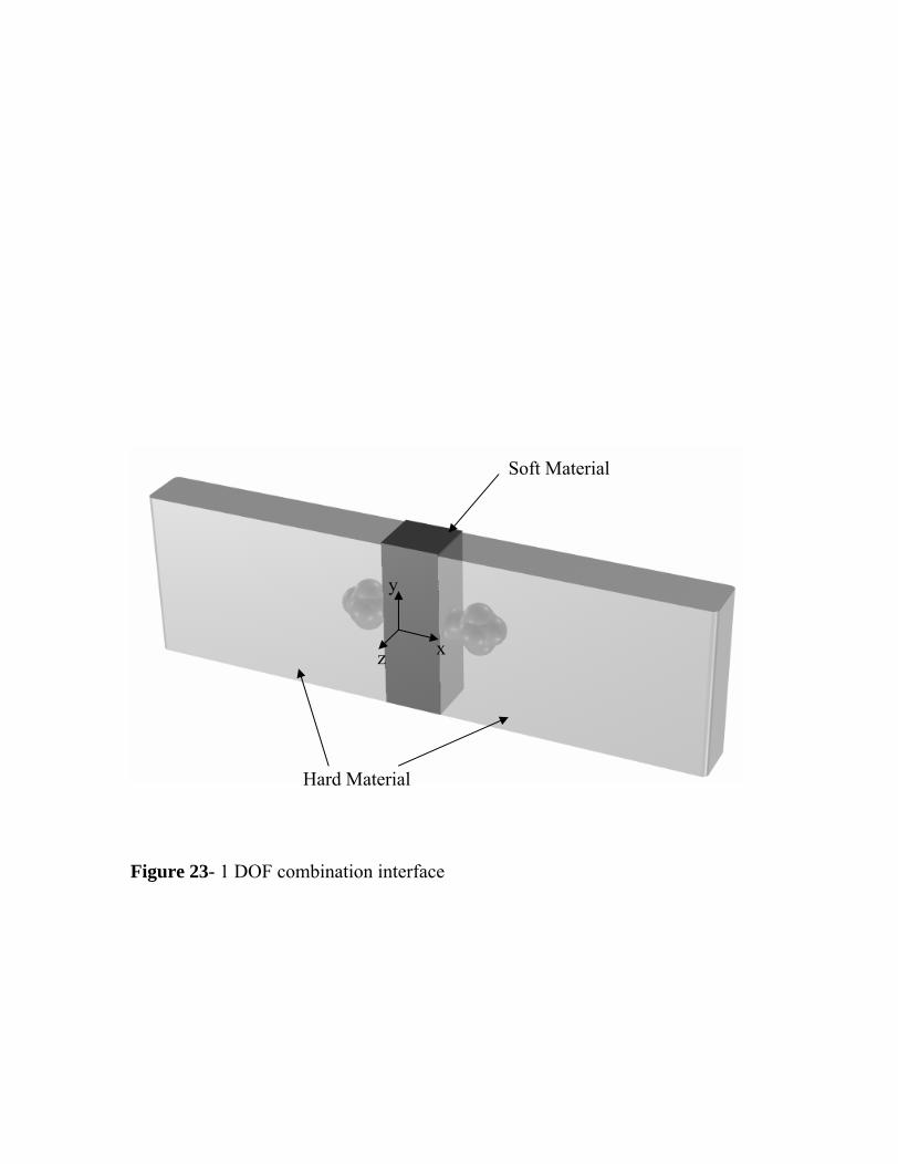
Figure 23- 1 DOF combination interface
x
y
z
Soft Material
Hard Material
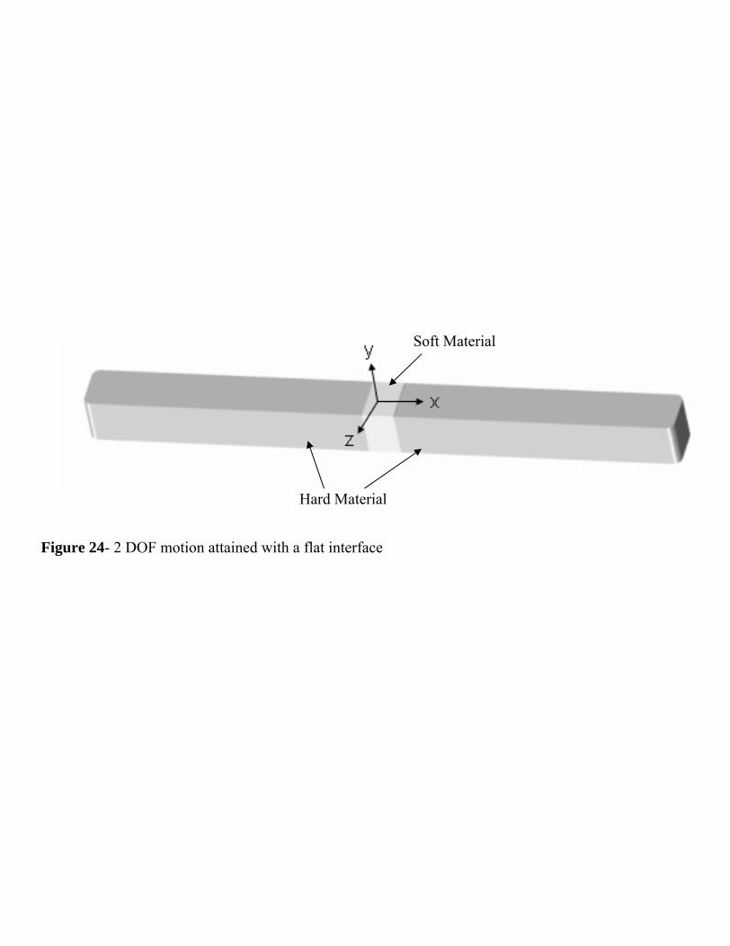
Figure 24- 2 DOF motion attained with a flat interface
Hard Material
Soft Material
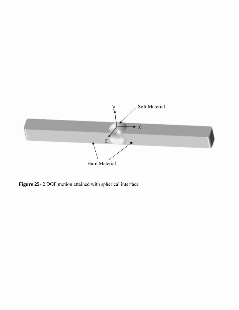
Figure 25- 2 DOF motion attained with spherical interface
Soft Material
Hard Material
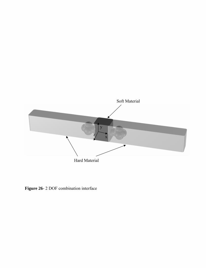
Figure 26- 2 DOF combination interface
x
y
z
Soft Material
Hard Material
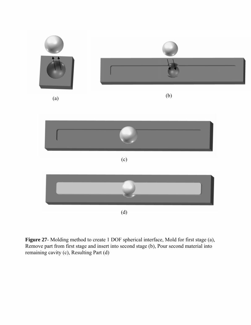
Figure 27- Molding method to create 1 DOF spherical interface, Mold for first stage (a), Remove part from first stage and insert into second stage (b), Pour second material into remaining cavity (c), Resulting Part (d)
(a) (b)
(c)
(d)
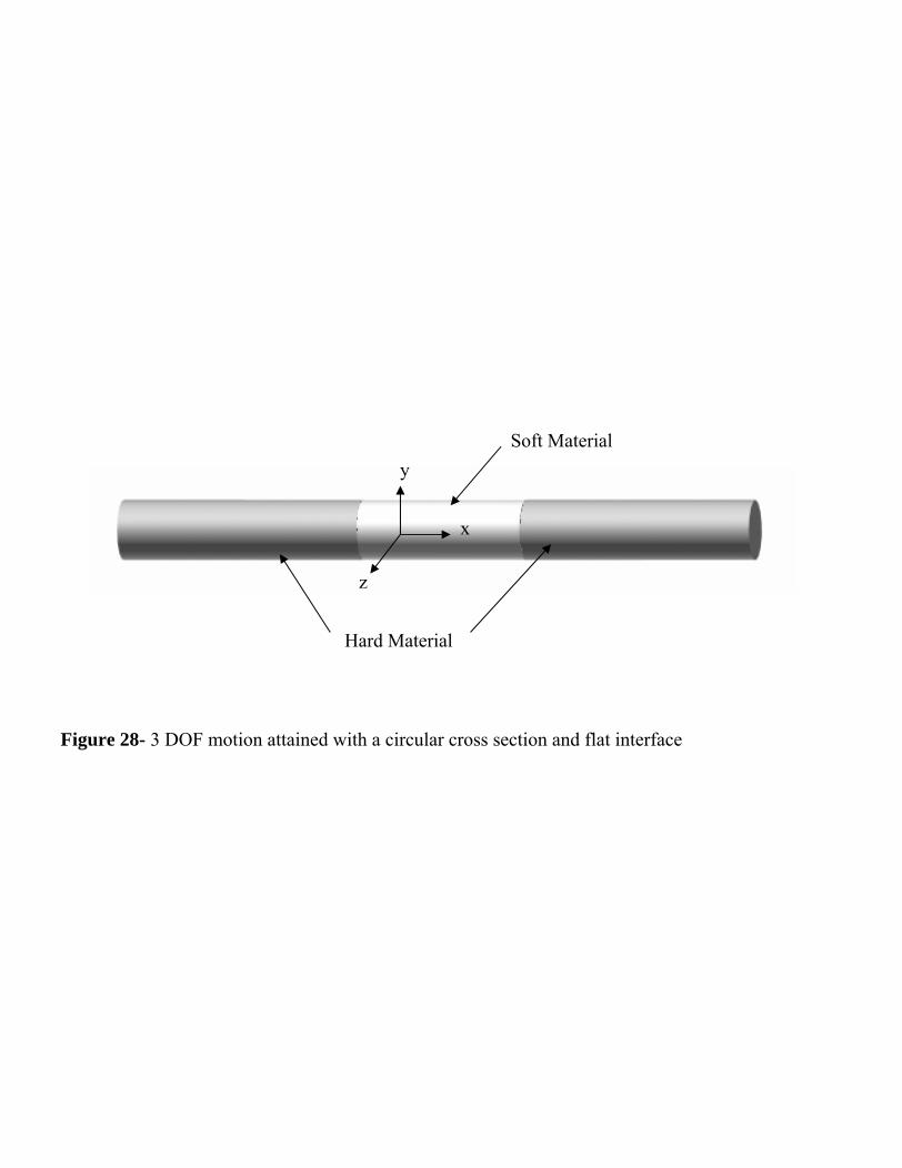
Figure 28- 3 DOF motion attained with a circular cross section and flat interface
x
y
z
Hard Material
Soft Material
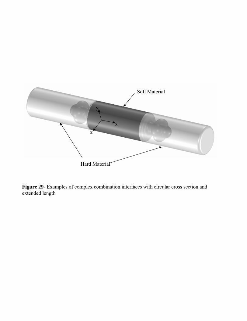
Figure 29- Examples of complex combination interfaces with circular cross section and extended length
x
y
z
Hard Material
Soft Material
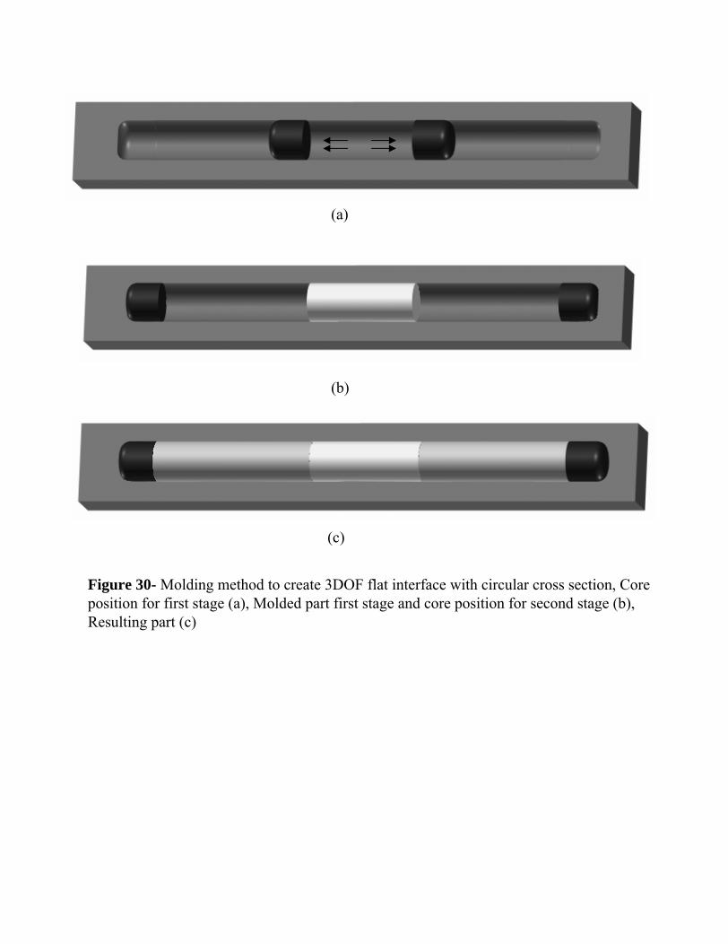
Figure 30- Molding method to create 3DOF flat interface with circular cross section, Core position for first stage (a), Molded part first stage and core position for second stage (b), Resulting part (c)
(a)
(b)
(c)
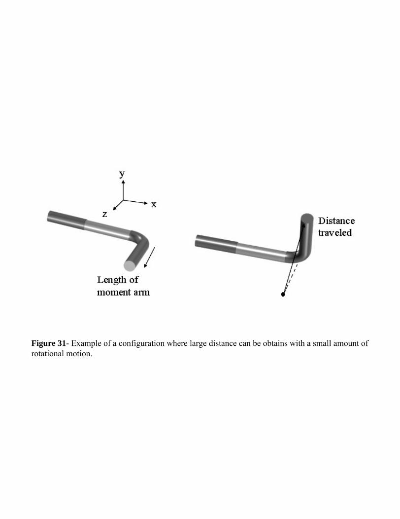
Figure 31- Example of a configuration where large distance can be obtains with a small amount of rotational motion.
(a) (b) (c)
Figure 32- Varying degrees of dimensional stability of the interface interstage, (a) highly deformed to (c) no deformation
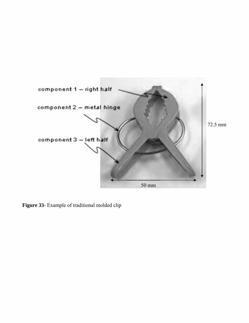
Figure 33- Example of traditional molded clip
50 mm
72.5 mm
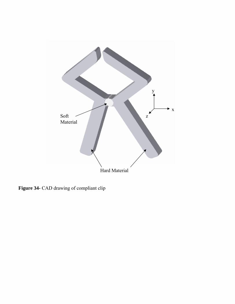
Figure 34- CAD drawing of compliant clip
x
y
zSoft Material
Hard Material
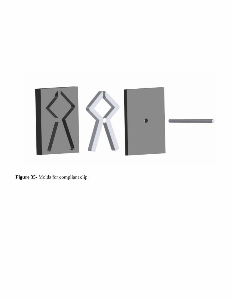
Figure 35- Molds for compliant clip
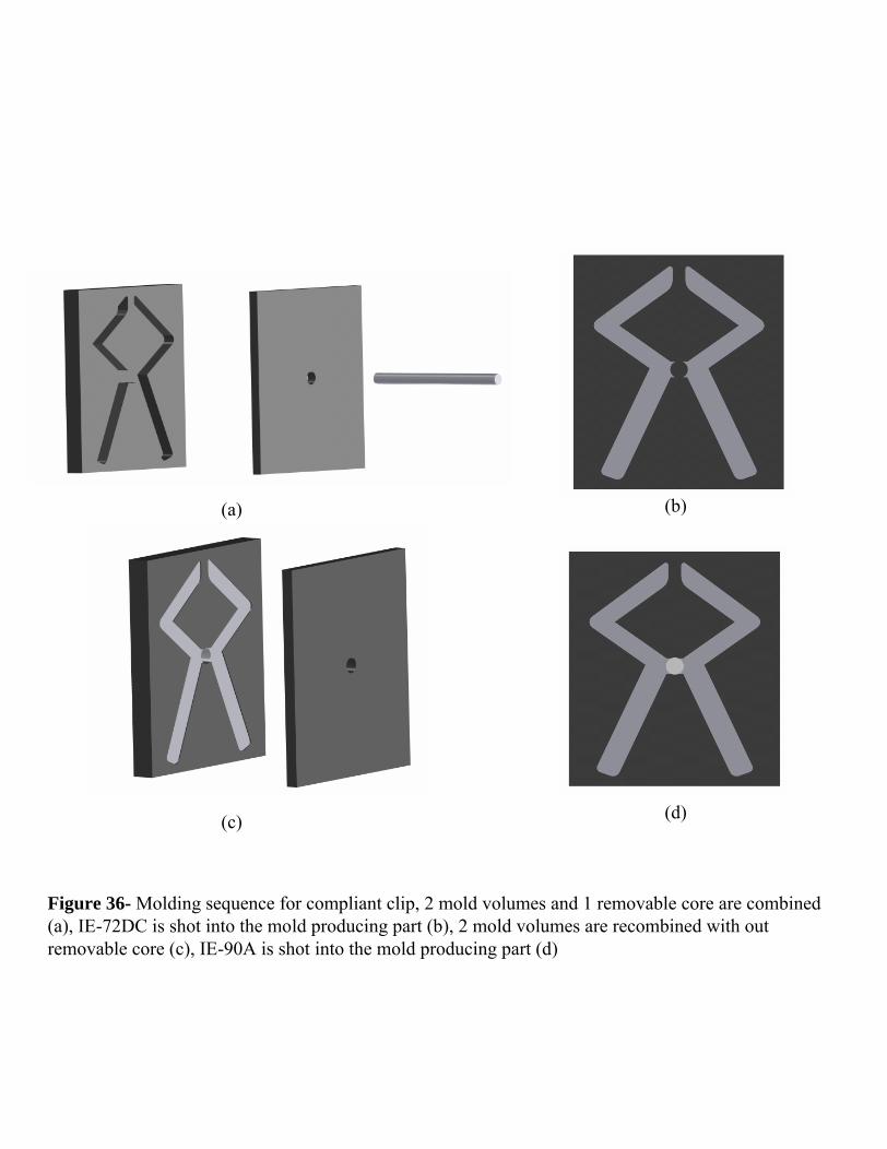
Figure 36- Molding sequence for compliant clip, 2 mold volumes and 1 removable core are combined (a), IE-72DC is shot into the mold producing part (b), 2 mold volumes are recombined with out removable core (c), IE-90A is shot into the mold producing part (d)
(a) (b)
(c) (d)
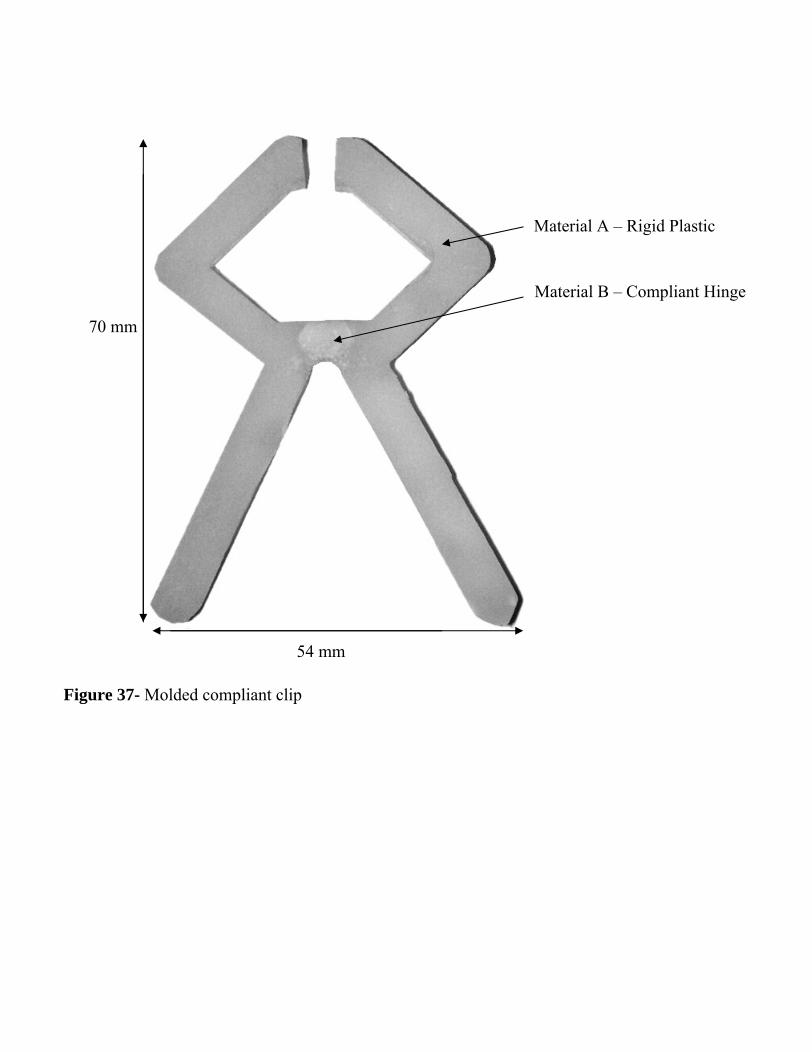
Figure 37- Molded compliant clip
Material A – Rigid Plastic
Material B – Compliant Hinge
54 mm
70 mm
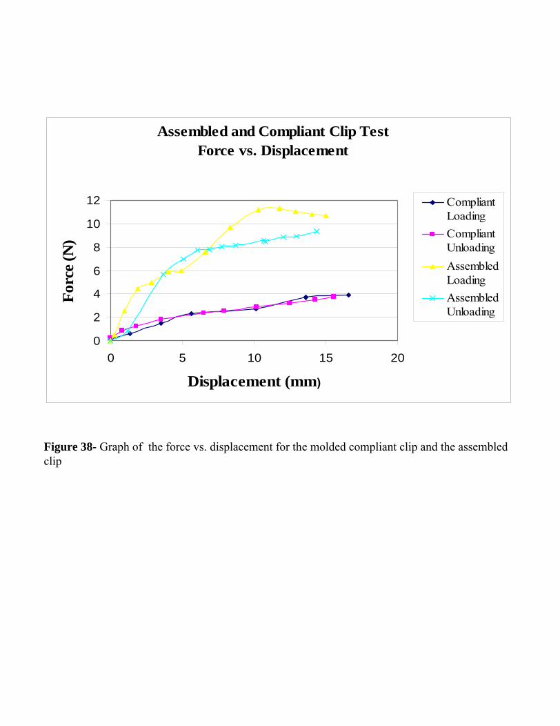
Figure 38- Graph of the force vs. displacement for the molded compliant clip and the assembled clip
Assembled and Compliant Clip TestForce vs. Displacement
0
2
4
6
8
10
12
0 5 10 15 20
Displacement (mm)
Forc
e (N
)
CompliantLoadingCompliantUnloadingAssembledLoadingAssembledUnloading
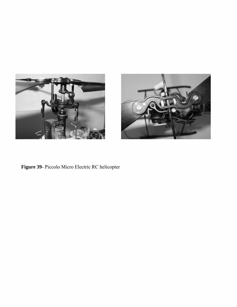
Figure 39- Piccolo Micro Electric RC helicopter
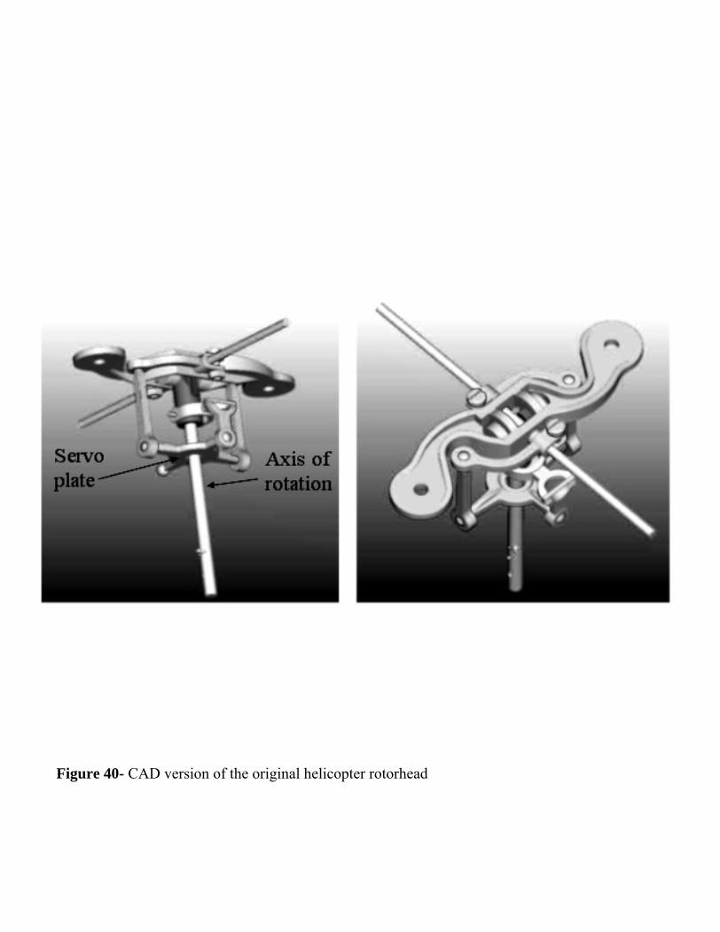
Figure 40- CAD version of the original helicopter rotorhead
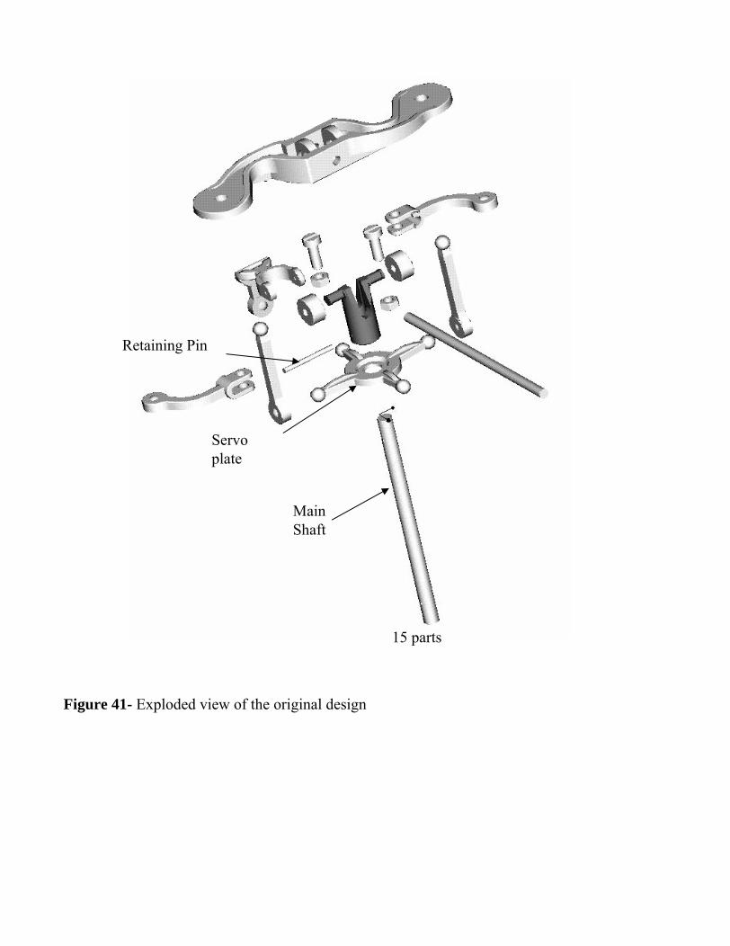
Figure 41- Exploded view of the original design
Main Shaft
Servoplate
Retaining Pin
15 parts
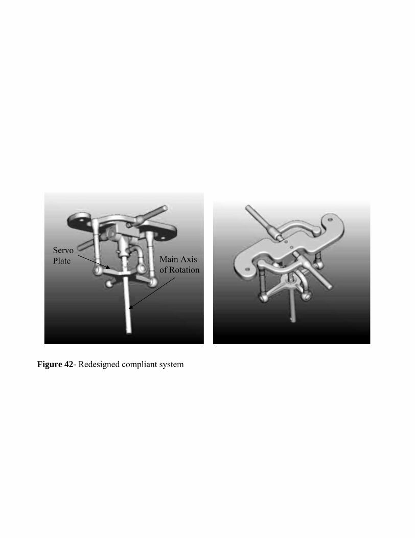
Figure 42- Redesigned compliant system
Servo Plate Main Axis
of Rotation
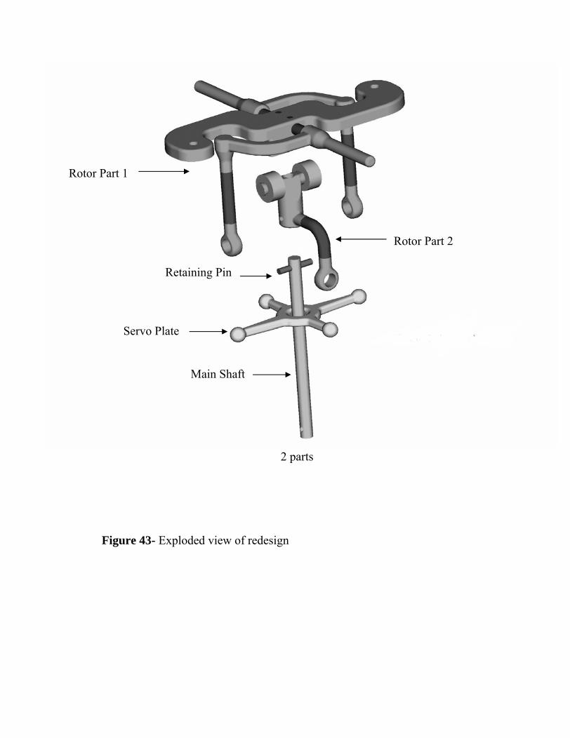
Figure 43- Exploded view of redesign
Rotor Part 1
Rotor Part 2
Main Shaft
Servo Plate
Retaining Pin
2 parts
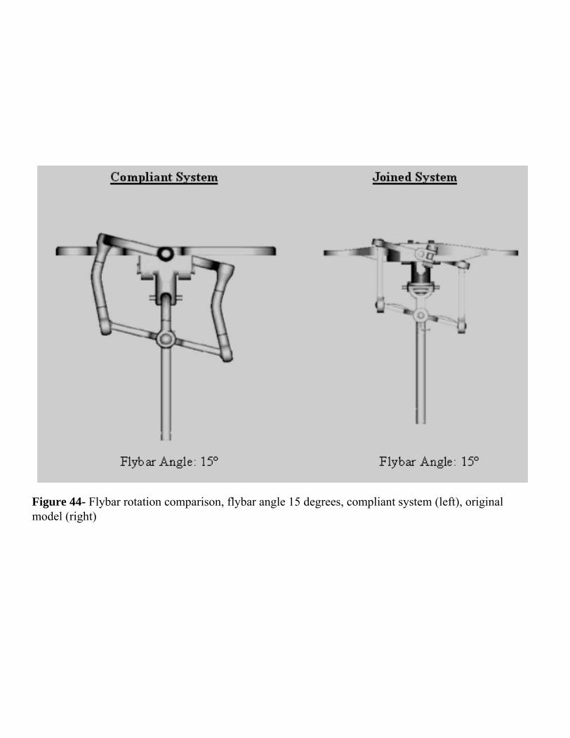
Figure 44- Flybar rotation comparison, flybar angle 15 degrees, compliant system (left), original model (right)
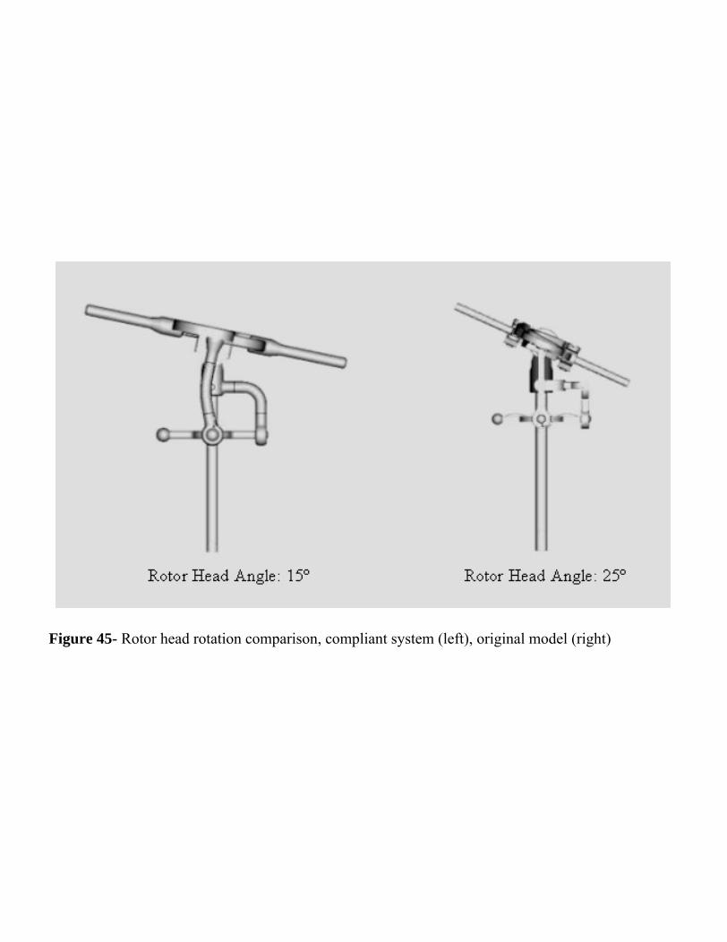
Figure 45- Rotor head rotation comparison, compliant system (left), original model (right)
(a)
(b)
Figure46- Mold joint breakdown
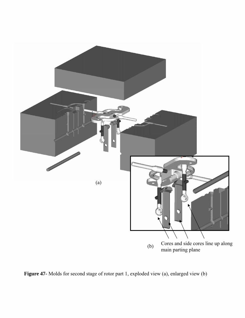
Figure 47- Molds for second stage of rotor part 1, exploded view (a), enlarged view (b)
(a)
(b) Cores and side cores line up along main parting plane
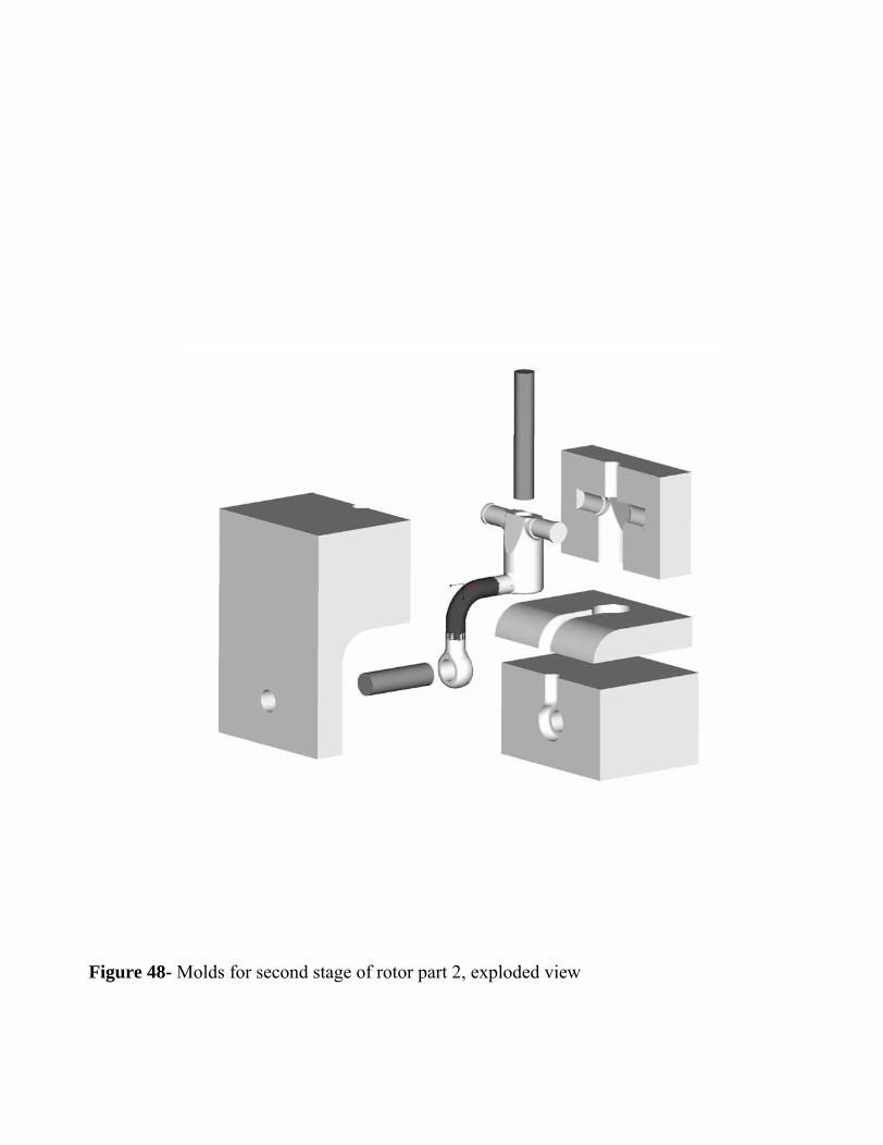
Figure 48- Molds for second stage of rotor part 2, exploded view
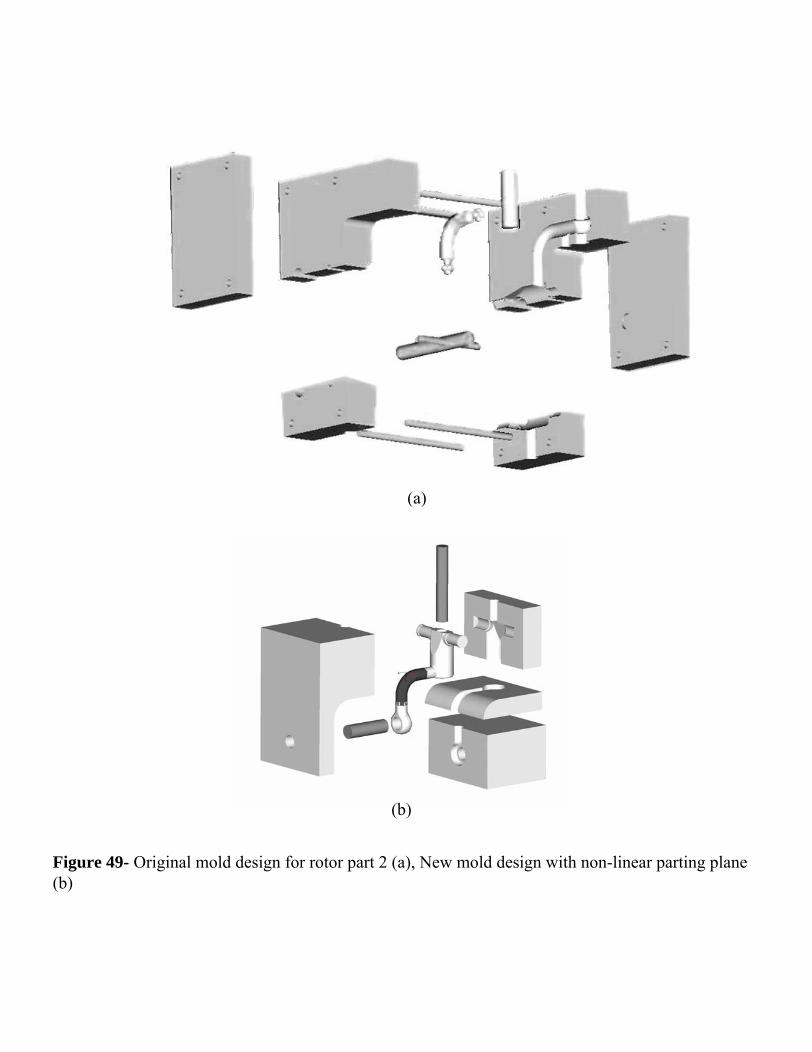
Figure 49- Original mold design for rotor part 2 (a), New mold design with non-linear parting plane (b)
(a)
(b)
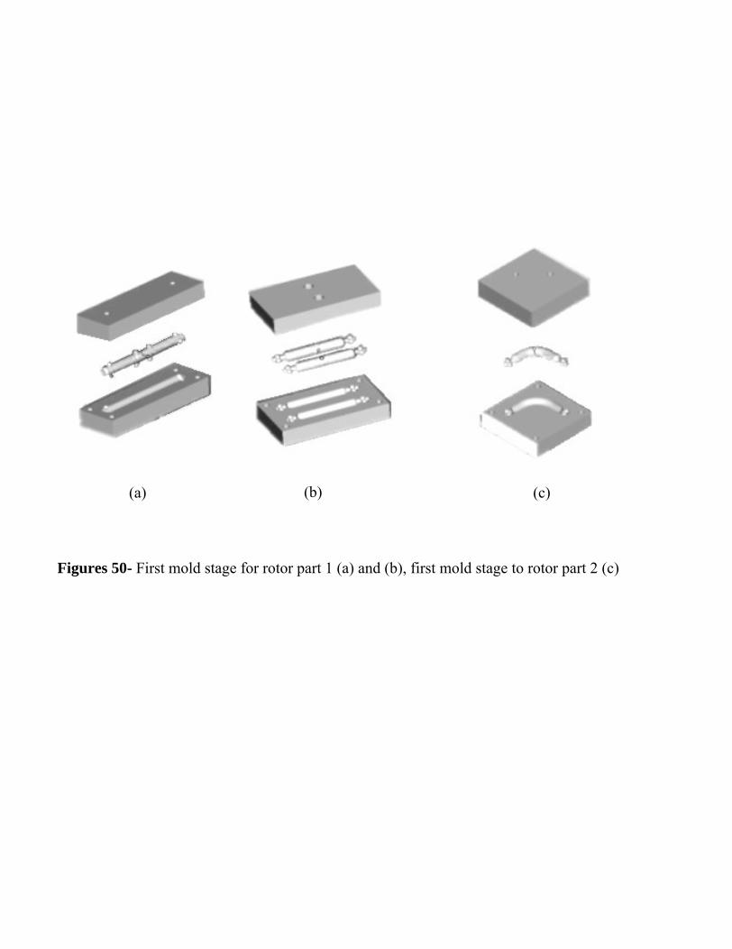
Figures 50- First mold stage for rotor part 1 (a) and (b), first mold stage to rotor part 2 (c)
(a) (b) (c)
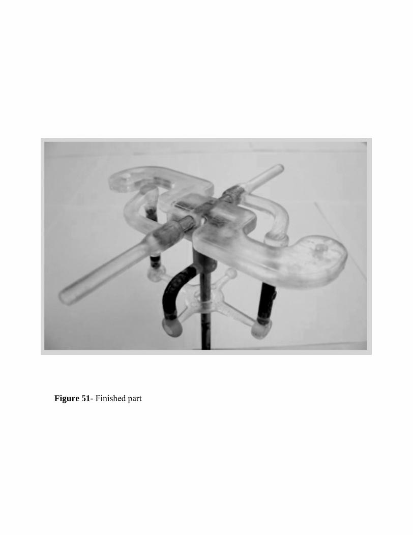
Figure 51- Finished part

Figure 52- Schematic of desired applied load and corresponding motion of the flybar
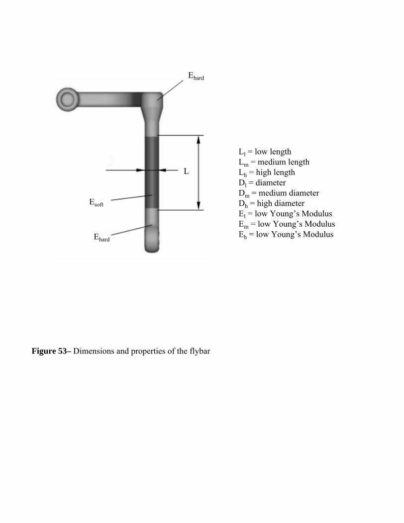
Ll = low lengthLm = medium lengthLh = high lengthDl = diameterDm = medium diameterDh = high diameterEl = low Young’s ModulusEm = low Young’s ModulusEh = low Young’s Modulus
Figure 53– Dimensions and properties of the flybar
Ehard
L
Esoft
Ehard
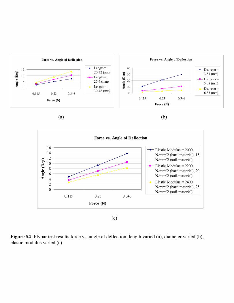
Figure 54- Flybar test results force vs. angle of deflection, length varied (a), diameter varied (b), elastic modulus varied (c)
Force vs. Angle of Deflection
0
5
10
15
0.115 0.23 0.346
Force (N)
Ang
le (D
eg)
Length =20.32 (mm)Length =25.4 (mm)Length =30.48 (mm)
Force vs. Angle of Deflection
0
10
20
30
40
0.115 0.23 0.346
Force (N)
Ang
le (D
eg)
Diameter =3.81 (mm)Diameter =5.08 (mm)Diameter =6.35 (mm)
Force vs. Angle of Deflection
02468
10121416
0.115 0.23 0.346
Force (N)
Ang
le (D
eg)
Elastic Modulus = 2000N/mm^2 (hard material), 15N/mm^2 (soft material)Elastic Modulus = 2200N/mm^2 (hard material), 20N/mm^2 (soft material)Elastic Modulus = 2400N/mm^2 (hard material), 25N/mm^2 (soft material)
(a) (b)
(c)


