
1
The Pain of Original Sin
Barry Eichengreen, Ricardo Hausmann and Ugo Panizza*
August 2003
* We are grateful to the Bank for International Settlements and to J.P. Morgan and in particular to Rainer Widera, Denis Pêtre and Martin Anidjar. We are grateful to Frank Warnock for pointing us to the US Treasury data, to Ernesto Stein for very useful collaboration in the early stages of this project and to Alejandro Riaño for excellent research assistance.
2
1. Introduction
If a country is unable to borrow abroad in its own currency � if it suffers from the
problem that we refer to as �original sin� � then when it accumulates a net debt, as
developing countries are expected to do, it will have an aggregate currency mismatch on
its balance sheet. Of course, such a country can take various steps to eliminate that
mismatch or prevent it from arising in the first place. Most obviously, it can decide not
to borrow. A financially autarchic country will have no currency mismatch because it
has no external debt, even though it still suffers from original sin as we define it. But this
response clearly has costs; the country in question will forgo all the benefits, in the form
of additional investment finance and consumption smoothing, offered by borrowing
abroad. Alternatively, the government can accumulate foreign reserves to match its
foreign obligations. In this case the country eliminates its currency mismatch by
eliminating its net debt (matching its foreign currency borrowing with foreign currency
reserves). But this too is costly: the yield on reserves is generally significantly below the
opportunity cost of funds.
All of this might seem relatively inconsequential. The currency denomination of
the foreign debt has not, until recently, figured prominently in theories of economic
growth and cyclical fluctuations. Macroeconomic stability, according to the conventional
wisdom, reflects the stability and prudence of a country�s monetary and fiscal policies.
The rate of growth of per capita incomes depends on rates of human and physical capital
accumulation and on the adequacy of the institutional arrangements determining how that
capital is deployed. Fine points like the currency in which a country�s foreign debt is

3
denominated, by comparison, are regarded as specialized concerns of interest primarily to
financial engineers.
In this chapter we show that neglect of this problem constitutes an important
oversight. In particular, we show that the composition of external debt � and specifically
the extent to which that debt is denominated in foreign currency � is a key determinant of
the stability of output, the volatility of capital flows, the management of exchange rates,
and the level of country credit ratings. We present empirical analysis demonstrating that
this �original sin� problem has statistically significant and economically important
implications, even after controlling for other conventional determinants of
macroeconomic outcomes. We show that the macroeconomic policies on which growth
and cyclical stability depend, according to the conventional wisdom, are themselves
importantly shaped by the denomination of countries� external debts.
Establishing the importance of original sin for the macroeconomic outcomes of
interest requires a precise measure of the phenomenon. Indeed, one reason why the
problem of debt denomination has not received the attention it deserves may be that
adequate information on its incidence and extent are not readily available. Thus, a
contribution of this chapter is to develop a series of numerical indicators of original sin.
In addition to demonstrating their importance for the macroeconomic variables relevant
to our argument, we present the indicators themselves, country by country, so they can be
used by other authors to analyze still other problems.
In Sections 2 and 3 of this chapter, we quantify the problem and characterize its
incidence. Section 4 analyzes its effects � what we characterize as the pain of original sin.

4
This is followed by a brief conclusion and an appendix where we report the results of a
battery of sensitivity analyses and present the underlying indicators.
2. Facts about Original Sin
Of the nearly $5.8 trillion in outstanding securities placed in international markets
in the period 1999-2001, $5.6 trillion was issued in 5 major currencies: the US dollar, the
euro, the yen, the pound sterling and Swiss franc. To be sure, the residents of the
countries issuing these currencies (in the case of Euroland, of the group of countries)
constitute a significant portion of the world economy and hence form a significant part of
global debt issuance. But while residents of these countries issued $4.5 trillion dollars of
debt over this period, the remaining $1.1 trillion of debt denominated in their currencies
was issued by residents of other countries and by international organizations. Since these
other countries and international organizations issued a total of $1.3 trillion dollars of
debt, it follows that they issued the vast majority of it in foreign currency. The
measurement and consequences of this concentration of debt denomination in few
currencies is the focus of this paper.
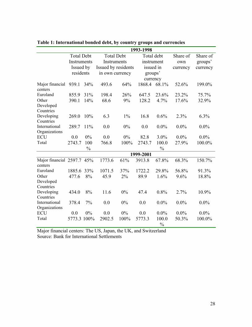
Table 1 presents data on the currency composition of bonded debt issued cross-
border between 1993 in 2001. �Cross-border� means that Table 1 excludes local issues.
We split the sample into two periods, demarcated by the introduction of the euro. The
figures are the average stock of debt outstanding during in each sub-period. The
information is organized by country groups and currencies of denomination. The first
country group, financial centers, is composed of the US, the UK, Japan, and Switzerland;
the second is composed of the Euroland countries; the third contains the remaining

5
developed countries; and the fourth is made up of the developing countries; we also
report data on bond issues by the international financial institutions (since these turn out
to be important below).
Column 1 presents the amount of average total stock of debt outstanding issued
by residents of these country groups. Column 2 shows the corresponding percentage
composition by country group. Columns 3 and 4 do the same for debt issued by residents
in their own currency, while columns 5 and 6 look at the total debt issued by currency,
independent of the residence of the issuer. Column 7 is the proportion of the debt that the
residents of each country group issued in their own currency (the ratio of column 3 to
column 1), while column 8 is the proportion of total debt issued in a currency relative to
the debt issued by residents of those countries (the ratio of column 5 to column 1).
Notice that while the major financial centers issued only 34 percent of the total
debt outstanding in 1993-1998, debt denominated in their currencies amounted to 68
percent of that total. In contrast, while other developed countries ex-Euroland issued fully
14 percent of total world debt, less than 5 percent of debt issued in the world was
denominated in their own currencies. Interestingly, in the period 1999-2001 � following
the introduction of the euro � the share of debt denominated in the currencies of other
developed countries declined to 1.6 percent. Developing countries accounted for 10
percent of the debt but less than one per cent of the currency denomination in the 1993-
1998 period. This, in a nutshell, is the problem of original sin.
When we look at the currency denomination of the debt issued by residents, we
see that residents of the major financial centers chose to denominate 68.3 percent of it in
their own currency in 1999-2001, while the residents of Euroland used the euro in 56.8

6
percent of their cross-border bond placements. This figure is substantially higher than the
23.2 percent which they chose to denominate in their own currency in 1993-1998, before
the introduction of the euro. In that earlier period, the other developed countries issued
17.6 percent of their debt in their own currencies, a number not too different from that for
the Euroland countries; in the recent period, however, this number has declined to 9.6
percent. The number for developing countries is an even lower 2.7 percent.
It is sometimes possible for countries to borrow in one currency and swap their
obligations into another. Doing so requires, however, that someone actually issue debt in
the domestic currency (otherwise there is nothing to swap). Column 8 takes this point on
board and is therefore a better measure of a country�s ability to borrow abroad in its own
currency than column 7, in the sense that when the ratio in column 8 is less than 1, it
indicates that there are not enough bonds to do the swaps needed to hedge the foreign
currency exposure of residents.
Column 8 reveals that in 1999-2001 the ratio of debt in the currencies of the
major financial centers to debt issued by their residents was more than 150 per cent.
(This, in a sense, is what qualifies them as financial centers.) This ratio drops to 91.3
percent for the Euroland countries, to 18.8 percent in the other developed countries
(down from 32.9 percent in the previous period), and to 10.9 percent for the developing
nations. Notice that after the introduction of the euro, Euroland countries narrow their
gap with the major financial centers while other developed countries converge towards
the ratios exhibited by developing nations.
Figure 1 plots the cumulative share of total debt instruments issued in the main
currencies (the solid line) and the cumulative share of debt instruments issued by the

7
largest issuers (the dotted line). The gap between the two lines is striking. While 87
percent of debt instruments are issued in the 3 main currencies (the US dollar, the euro
and the yen), residents of these three countries issue only 71 percent of total debt
instruments. The corresponding figures for the top five currencies, 97 and 83 percent,
respectively, tell the same story.
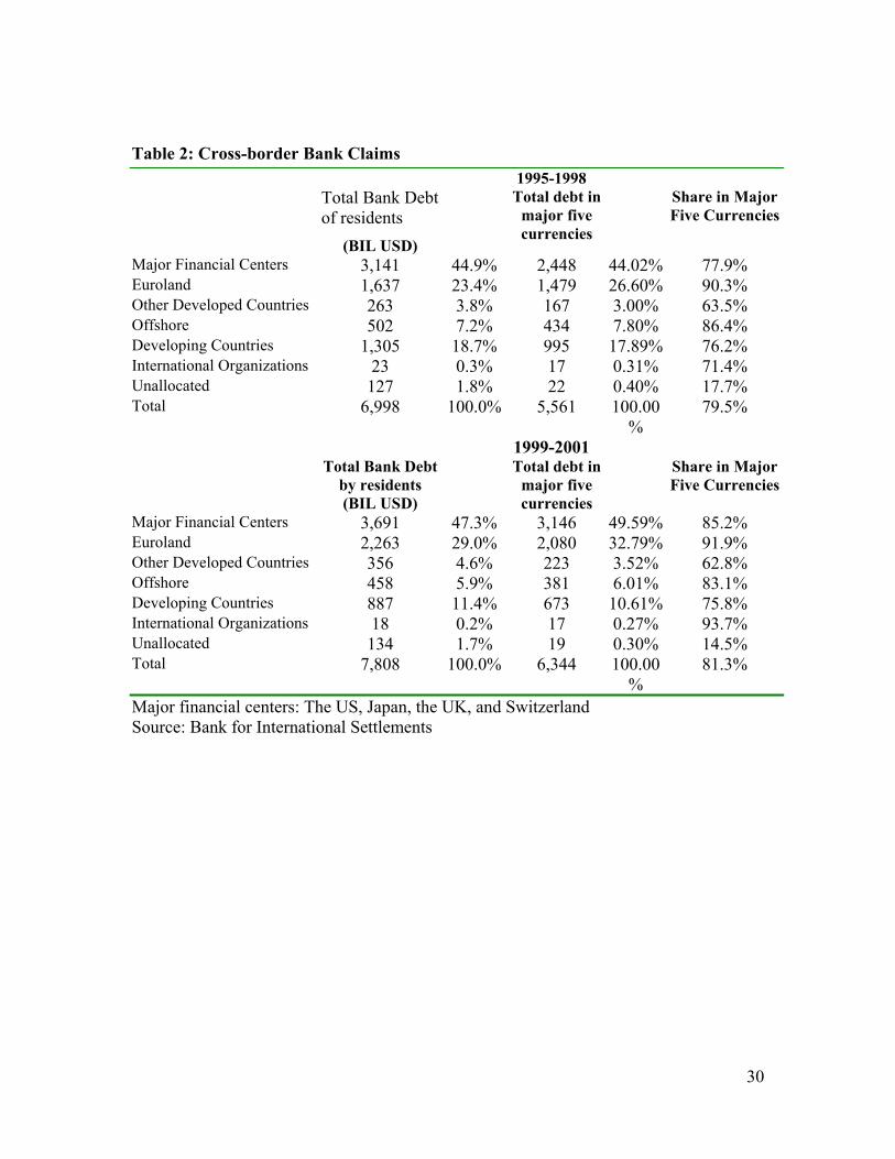
Table 2 presents similar information for cross-border claims by international
banks reporting to the Bank for International Settlements. These data only distinguish the
five major currencies (US dollar, euro, Swiss franc, British pound, and Japanese yen) and
an �other currency� category. The table shows that of $7.8 trillion in cross-border bank
claims, 81 percent are denominated in the 5 major currencies. While we cannot know
how much is actually issued in each borrower�s currency, we can safely say that the bulk
of the debt in the developing world and in the developed countries outside the issuers of
the major currencies is also in foreign currency.
One possible problem with the data of Table 1 is that it only captures cross-border
bond issuance and does not capture the nationality of the bondholder, only the place of
issue. So, it may be the case that countries do their local currency funding in the local
market and their foreign currency funding abroad. Foreigners willing to hold domestic
currency bonds would just purchase them in the local markets. These domestically issued
but foreign owned domestic currency bonds would not be included in Table 1. To address
this issue we look at the currency composition of the international securities held by US
residents, independently of the place of issue.
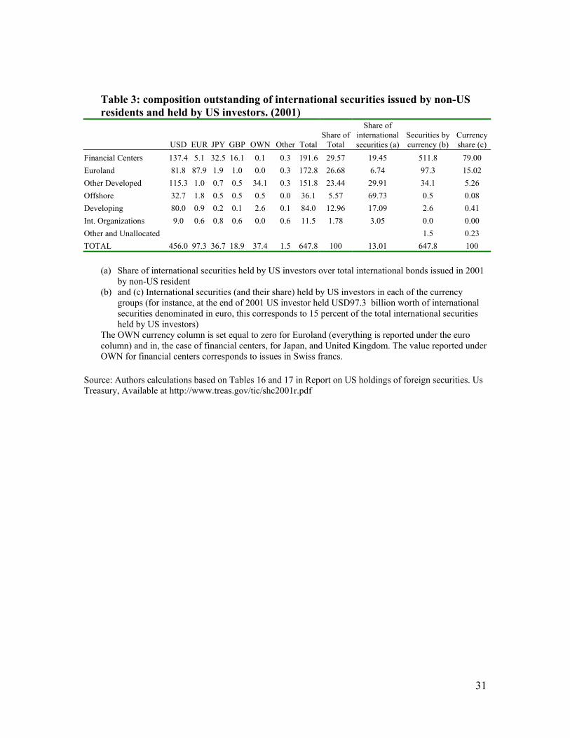
According to the US Treasury (Table 3), these securities amounted to USD 647
billion at the end of 2001. However, of these securities USD 456 billion or 70.4 percent

8
were denominated in US dollars. This indicates that the willingness of US investors to
expose themselves to foreign credit risk is significantly higher than their willingness to
expose themselves to foreign currency risk: they hold more claims on foreigners than
claims in foreign currency. Moreover, if we include the exposure to the euro, the yen and
the British pound and the Canadian dollar, the total foreign exposure of US investors
denominated in major currencies amounts to 97 percent of the total. In the case of
developing countries, while US investors held USD 84 billion in securities issued by
developing countries, only 2.6 billion (or 3.1 percent) was denominated in local currency.
The message of Table 3 is similar to that of Table 1: global investors denominate their
claims predominantly in very few currencies. The willingness to hold foreign securities is
significantly larger than the willingness to hold them in foreign currency, except for a
few major currencies.
All this points to the fact that original sin is a global phenomenon. It is not
limited to a small number of problem countries. It seems to be associated with the fact
that the vast majority of the world�s financial claims are denominated in a small set of
currencies. In turn this suggests that the problem may have something to do with
observed patterns of portfolio diversification � or its absence. We develop this point in
Chapter 9.
3. Measuring Original Sin
To develop indices of original sin, we use the data on securities and bank claims
used to construct Tables 1 and 2. We start with the securities data set, which provides a
full currency breakdown.

9
Our first indicator of original sin (OSIN1) is one minus the ratio of the stock of
international securities issued by a country in its own currency to the total stock of
international securities issued by the country. That is,1
iiiOSIN i country by issued Securities
currency in country by issued Securities11 −=
Thus, a country that issues all its securities in own currency would get a zero, while a
country that issues all of them in foreign currency would get a 1 (the higher the value, the
greater the sin). We also compute a variant of OSIN1 by using the data on security
holding by US investors (USSIN1).
OSIN1 has two drawbacks. First, it only covers securities and not other debts.
Second, it does not take account of opportunities for hedging currency exposures through
swaps. We deal with these issues next. Consider the following ratio:
iiINDEXAi country by issued Loans Securities
currenciesmajor in country by issued LoansSecurities+
+=
INDEXA has the advantage of increased coverage. (It also has the disadvantage
of not accounting for the debt denominated in foreign currencies other than the majors;
we address this problem momentarily). To capture the scope for hedging currency
exposures via swaps, we also consider a measure of the form:
iiINDEXBi country by issued Securities
currency in Securities1−=
INDEXB accounts for the fact, discussed above, that debt issued by other
countries in one�s currency creates an opportunity for countries to hedge currency
1 We follow Hausmann et al. (2001) but extend their sample from 30 to 90 countries and update it to the end of 2001.

10
exposures via the swap market. Notice that this measure can take on negative values, as it
in fact does for countries such as the US and Switzerland, since there is more debt issued
in their currency than debt issued by nationals. However, these countries cannot hedge
more than the debt they have. Hence, they derive scant additional benefits from having
excess opportunities to hedge. We therefore substitute zeros for all negative numbers,
producing our third index of original sin:
−= 0,
country by issued Securitiescurrency in Securities1max3
iiOSIN i
We are now in a position to refine INDEXA. Recall that INDEXA understates
original sin by assuming that all debt that is not in the 5 major currencies is denominated
in local currency. This may be a better approximation for countries with some capacity to
issue debt in their own currencies. However, if this is so, it should be reflected in OSIN3
because it means that someone � either a resident or a foreign entity � might have been
able to float a bond denominated in that currency. If this is not the case, this provides
information about the likelihood that the bank loans not issued in the 5 major currencies,
were denominated in some other foreign currency. We therefore replace the value of
INDEXA by that of OSIN3 in those cases where the latter is greater than the former.2
Hence we propose to measure OSIN2 as:
)3,max(2 iii OSININDEXAOSIN =
Notice that OSIN2 ≥ OSIN3 by construction and that, in most cases, OSIN1 ≥
OSIN2.
2 If the composition of the bank debt was the same as that of securities then OSIN3 should be smaller than INDEXA, since it includes not only debt issued by residents but also that issued by foreigners. When OSIN3 is greater than INDEXA, it is informative of a potential underestimate of original sin.
11
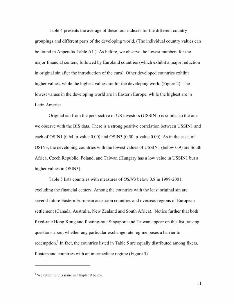
Table 4 presents the average of these four indexes for the different country
groupings and different parts of the developing world. (The individual country values can
be found in Appendix Table A1.) As before, we observe the lowest numbers for the
major financial centers, followed by Euroland countries (which exhibit a major reduction
in original sin after the introduction of the euro). Other developed countries exhibit
higher values, while the highest values are for the developing world (Figure 2). The
lowest values in the developing world are in Eastern Europe, while the highest are in
Latin America.
Original sin from the perspective of US investors (USSIN1) is similar to the one
we observe with the BIS data. There is a strong positive correlation between USSIN1 and
each of OSIN1 (0.64, p-value 0.00) and OSIN3 (0.50, p-value 0.00). As in the case, of
OSIN3, the developing countries with the lowest values of USSIN1 (below 0.9) are South
Africa, Czech Republic, Poland, and Taiwan (Hungary has a low value in USSIN1 but a
higher values in OSIN3).
Table 5 lists countries with measures of OSIN3 below 0.8 in 1999-2001,
excluding the financial centers. Among the countries with the least original sin are
several future Eastern European accession countries and overseas regions of European
settlement (Canada, Australia, New Zealand and South Africa). Notice further that both
fixed-rate Hong Kong and floating-rate Singapore and Taiwan appear on this list, raising
questions about whether any particular exchange rate regime poses a barrier to
redemption.3 In fact, the countries listed in Table 5 are equally distributed among fixers,
floaters and countries with an intermediate regime (Figure 3).
3 We return to this issue in Chapter 9 below.

12
Original sin is also persistent, to a surprising extent. Flandreau and Sussman in
Chapter 6 below present a three-way classification of original sin circa 1850, based on
whether countries placed bonds in local currency, indexed their debt to gold (included
gold clauses in their debts), or did some of both. Table 6 shows the mean value of OSIN3
in the 1993-1998 period for each of the three groups distinguished by Flandreau and
Sussman. OSIN3 is highest today in the same countries that had gold clauses in their debt
in the 19th century (average 0.86) and lowest for countries that issued domestic debt
(average 0.34) and intermediate in countries that issued both gold-indexed and domestic-
currency debt (average 0.53); hence, there is a high correlation between original sin then
and now. The standard t test suggests that countries that exclusively issued debt with gold
clauses in the 1850s suffer from significantly higher levels of original sin today than
either countries that issued both gold-indexed and domestic-currency debt (p-value =
0.016) or those that issued exclusively in local currency (p-value = 0.000).
In their original formulation, Eichengreen and Hausmann (1999) defined original
sin as �a situation in which the domestic currency cannot be used to borrow abroad, or to
borrow long term, even domestically [emphasis added]. While the focus of this book and
this chapter is the inability to borrow abroad in domestic currency (what we call
international original sin), we also computed an index for the capacity of a country to
borrow at long maturities domestically (which we refer to as domestic original sin). There
are two reasons for deriving such an index. First of all, it would be important to know to
what extent these two issues are related or are in fact two different types of issues.
Second, it has been argued that creating a domestic market in own currency is a necessary

13
condition for inducing foreigners to use a country�s currency (Tirole, 2002). We would
like to shed some light on these issues both here and in Chapter 9.
Our main source of information is J.P. Morgan�s (2002, 2000, 1998) �Guide to
Local Markets� that reports detailed information on domestically traded public debt for
22 emerging market countries. J.P. Morgan also provides information on the presence of
domestic private debt instruments and shows that in most countries (the exceptions being
Singapore, South Korea, Taiwan, and Thailand) this is a negligible component of traded
debt.
J.P. Morgan reports data on total outstanding domestic government bonds and the
main characteristics (total amount, maturity, currency, and coupon) of the various
government bonds present in each market. We classify the bonds listed by J.P. Morgan
according to their maturity, currency, and coupon (fixed and indexed rate). In particular,
we divide outstanding government bonds into 5 categories: (i) long-term domestic
currency fixed rate (DLTF); (ii) short-term domestic currency fixed rate (DSTF); (iii)
long-term (or short-term) domestic currency debt floating rate debt, i.e. indexed to an
interest rate (DLTII); (iv) long-term domestic currency debt indexed to the price level
(DLTIP); and (v) foreign currency debt (FC). Using the above information, we compute
the following indicator of domestic Original Sin:4
DLTIPDLTIIDSTFDLTFFCDLTIIDSTFFCDSIN
++++++=
4 Hausmann and Panizza (2003) discuss alternative indicators of domestic original sin.
14
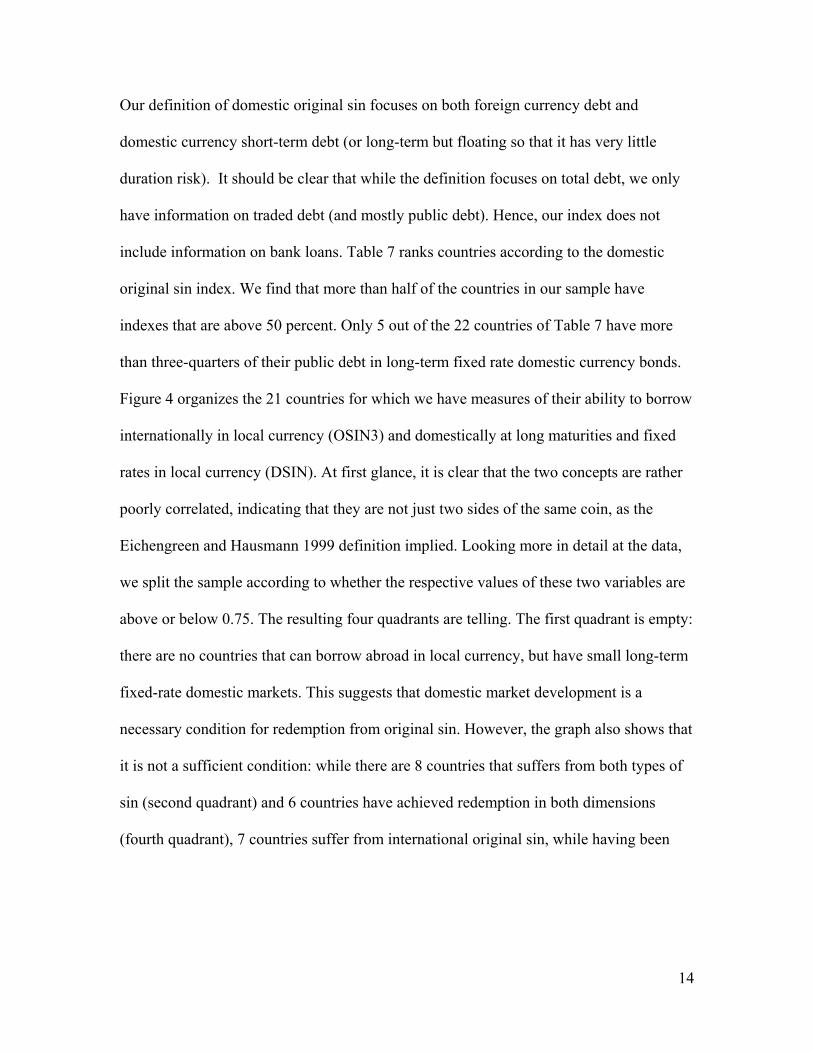
Our definition of domestic original sin focuses on both foreign currency debt and
domestic currency short-term debt (or long-term but floating so that it has very little
duration risk). It should be clear that while the definition focuses on total debt, we only
have information on traded debt (and mostly public debt). Hence, our index does not
include information on bank loans. Table 7 ranks countries according to the domestic
original sin index. We find that more than half of the countries in our sample have
indexes that are above 50 percent. Only 5 out of the 22 countries of Table 7 have more
than three-quarters of their public debt in long-term fixed rate domestic currency bonds.
Figure 4 organizes the 21 countries for which we have measures of their ability to borrow
internationally in local currency (OSIN3) and domestically at long maturities and fixed
rates in local currency (DSIN). At first glance, it is clear that the two concepts are rather
poorly correlated, indicating that they are not just two sides of the same coin, as the
Eichengreen and Hausmann 1999 definition implied. Looking more in detail at the data,
we split the sample according to whether the respective values of these two variables are
above or below 0.75. The resulting four quadrants are telling. The first quadrant is empty:
there are no countries that can borrow abroad in local currency, but have small long-term
fixed-rate domestic markets. This suggests that domestic market development is a
necessary condition for redemption from original sin. However, the graph also shows that
it is not a sufficient condition: while there are 8 countries that suffers from both types of
sin (second quadrant) and 6 countries have achieved redemption in both dimensions
(fourth quadrant), 7 countries suffer from international original sin, while having been

15
redeemed on the domestic front (third quadrant).5 In Chapter 9 we discuss the causes of
this pattern and the unconventional role played by capital controls6.
4. The Pain
Original sin has important consequences. Countries with original sin that have net
foreign debt will have a currency mismatch on their national balance sheets. Movements
in the real exchange rate will then have aggregate wealth effects.7 This makes the real
exchange rate a relevant price in determining the capacity to pay. Since the real exchange
rate is quite volatile and it tends to depreciate in bad times, original sin significantly
lowers the creditworthiness of a country. Moreover, the wealth effects limit the
effectiveness of monetary policy, as expansionary policies may weaken the exchange
rate, cause a reduction in net worth and will thus be either less expansionary or even
contractionary (Aghion, Bacchetta and Banerjee 2001, Céspedes, Chang and Velasco in
Chapter 2 of this volume). This renders central banks less willing to let the exchange rate
move, and they respond by holding more reserves and aggressively intervening in the
foreign exchange market or adjusting short-term interest rates (Hausmann, Panizza and
Stein, 2001, Calvo and Reinhart, 2002). The existence of dollar liabilities also limits the
ability of central banks to avert liquidity crises in their role as lenders of last resort
(Chang and Velasco, 2000). And, dollar-denominated debts and the associated volatility
5 In what remains, we will refer to original sin as referring exclusively to its international dimension, i.e. to the ability to borrow abroad in local currency. 6 A more in depth discussion can be found in Hausmann and Panizza (2003). 7 Governments can of course close the economy to foreign borrowing or accumulate international reserves sufficient to match the foreign-currency obligation (in which case it will also not have a net foreign debt). Our point is that an aggregate mismatch is unavoidable when a country suffers from original sin and there is a net foreign debt. Note also that the wealth effect may be smaller in countries with a larger tradable sector, this is why most of our regressions control for openness.

16
of domestic interest rates heighten the uncertainty associated with public debt service,
thus lowering credit ratings.
Given these facts, it is no surprise that countries afflicted by original sin have a
hard time achieving domestic economic stability. Their incomes are more variable and
their capital flows more volatile than those of countries free of the phenomenon. Since
financial markets know that inability to borrow abroad in the domestic currency is a
source of financial fragility, developing countries burdened with original sin are charged
an additional risk premium when they borrow, forcing them to skate closer to the edge of
solvency. A shock to the exchange rate can then cause asset prices to move adversely,
tipping them over the precipice. But if countries attempt instead to minimize these risks
by limiting their recourse to foreign sources of funding, they may then be starved of the
finance needed to underwrite their growth. The process of economic and financial
development will be slowed. Countries in this situation thus face a Hobson�s choice.
Original sin and fiscal solvency
It has been amply recognized that developing countries tend to be more volatile
than industrial countries in the sense that they have a more unstable rate of GDP growth
(IDB, 1995, Hausmann and Gavin 1996). Table 8 shows that their GDP growth is more
than twice as volatile as that of industrial countries: 5.8 percent per annum instead of 2.7.
However, if a country�s debt is denominated in foreign currency � say US dollars � its
capacity to pay will be related, not to the value of its GDP in constant local currency units
(LCU), but in US dollar terms. Table 8 shows that the volatility of changes in real US$
GDP is almost 3 times higher than in LCU for developing countries. Hence, the typical
industrial country without original sin would face a relevant volatility of 2.7 percent per

17
annum, while the typical developing country with original sin would face a relevant
volatility of 13 percent.
The greater relevant volatility in the capacity to pay comes from the fact that
original sin makes the real exchange rate matter for debt service and this variable is very
volatile in developing countries. Table 9 presents the volatility of the real exchange rate
for a sample of developed and developing countries. The volatilities are normalized to be
equal to 1 for the sample as a whole. The table clearly shows that the volatility of the real
exchange rate is between 2 and 3 times higher in developing countries. Hence, not only
does the real exchange rate matter for debt service in countries with original sin, but in
addition, the real exchange rate in these countries tends to be significantly more volatile.
Analysts often argue that a volatile real exchange rate does not matter if the debt
is sufficiently long term. If purchasing power parity holds in the long run, then deviations
of the real exchange rate should not be very long-lived and a country�s solvency should
not be much affected by relatively temporary movements in the real exchange rate.
Markets will not change their minds about the solvency of a country based on short term
movements of the real exchange rate. However, Table 8 shows that the volatility of
movements in the five-year moving average of the real multilateral exchange rate is very
high. The table calculates the percentage gap between the maximum and the minimum
value of a 5 year moving average of the real exchange rate for a sample of developed and
developing countries for the period between 1980 and 2000. The table indicates that the
5-year moving average moved by more than 60 percent in the average developing

18
country, more than three times the magnitude of industrial countries8. Said differently,
the 5-year average value of the debt to GDP ratio would have moved by more than 50
percent in the typical developing countries through real exchange rate valuation changes
alone! Table 9 shows that the greater volatility of the real exchange rate in developing
countries is as much of a feature at 5 years than at 1 year and that it has remain the same
in the 1980s and 1990s.
Another way to look at this data is by studying the events in which there has been
a large decline in the capacity to pay foreign debt. Table 10 shows the occasions in which
the dollar value of GDP over a two-year period fell by more than 30 percent9. Two facts
clearly emerge from the table: the events identified tend to capture many of the recent
debt crises. More importantly, while the average decline in dollar GDP for this sample of
countries was 46 percent, the decline in GDP in local currency units was less than a
twentieth of that. The collapse in the capacity to pay is more related to real exchange rate
movements than to output declines.
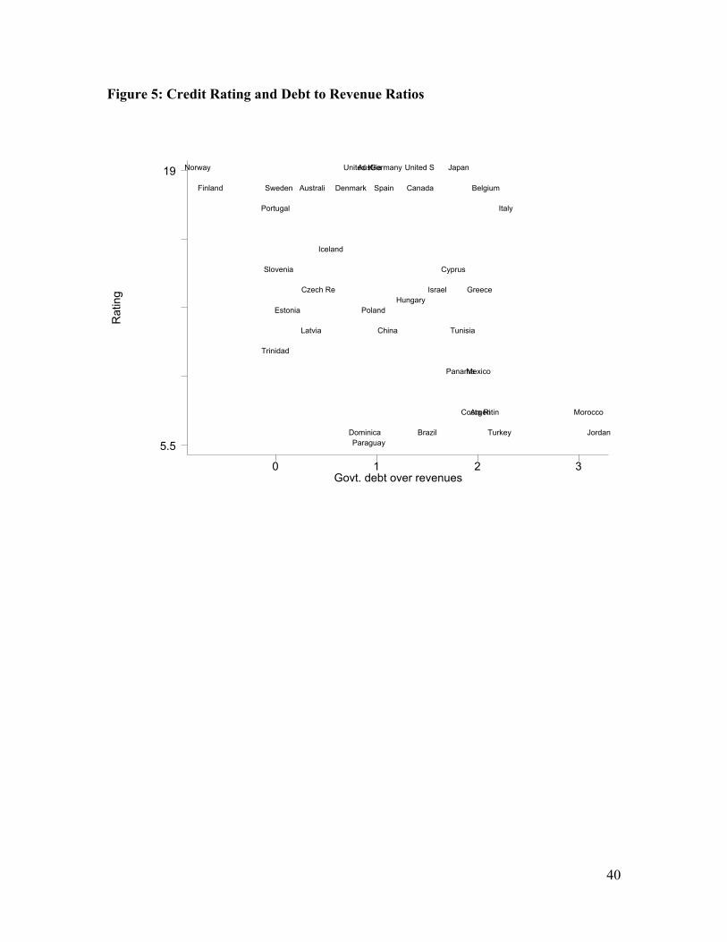
One implication of this analysis is that countries suffering from original sin
should be significantly riskier than countries without this burden, after controlling for
other determinants of creditworthiness such as debt ratios. This may help explain the poor
predictive capacity of fiscal fundamentals such as the debt to tax revenue ratio as a
8 The multilateral exchange rate tends to be smaller than their bilateral real exchange rate vis a vis the US dollar, especially for industrial countries. 9 We use a two-year period in order to take account of the fact that a large depreciation will have a different impact on the one-year decline in GDP depending on the month in which it takes place. A two-year period helps smooth out this effect.

19
determinant of credit rating, as is clear from Figure 5.10 Countries like Brazil, Argentina,
Turkey and Mexico had a debt to tax ratio that was broadly similar or in fact lower than
those of the Italy, Belgium, the US, Canada or Spain while their credit rating could not be
more different.11 As argued in Hausmann (2003), original sin lowers evaluations of
solvency because it heightens the dependence of debt service on the evolution of the
exchange rate, which is more volatile and may be subject to crises and crashes.
To test this hypothesis, we regress foreign-currency credit rating of countries on
two standard measures of fiscal fundamentals -- public debt as a share of GDP and public
debt as a share of tax revenues-- on the level of development, on the magnitude of the
foreign debt (SHARE) and on original sin. The equations are estimated by weighted
double-censored Tobit. The results, in Table 11, show a large and statistically significant
effect of original sin on credit ratings.12 Redemption (the total elimination of original sin)
is associated with an improvement of ratings by about five notches. This effect is strong
and present even though we control for the level of economic development, as captured
by the real GDP per capita and for the magnitude of the public debt measured either as a
share of GDP or as a share of tax revenues.
Hence, original sin helps explain why countries suffer from creditworthiness
problems: it is not due to their incapacity to limit debt accumulation; it is that the
10 The debt to GDP ratio is an even worse predictor. However, it can be argued that public debt is serviced out of the portion GDP that the government can tax. Since tax revenue to GDP ratios are lower in developing countries they should therefore have a lower debt to GDP ratio for the same rating. 11 We use the ratings from Standard and Poor�s. We converted the S&P rating into a numerical variable by adopting the following criterion. Selective default = 0, C=2, CC=2.5, CCC= 3, B-=4, and each extra upgrade one point. The maximum is 19 that corresponds to AAA. 11 We test whether the effect of credit rating was due to non-linearities around the investment grade threshold but find no evidence for this hypothesis. 12 These results are robust to alternative definitions of original sin, also as shown in Appendix Table A4.

20
structure of that debt makes them risky at low levels of debt that are consistent with a
AAA rating in other countries.
Original sin and nominal exchange rate volatility
We will now explore the relationship between the management of monetary and
exchange rate policy and the presence of original sin. We posit that countries that suffer
from this phenomenon will be less willing to allow their exchange rate to fluctuate. There
are no widely accepted indicators of exchange rate flexibility. We will therefore employ
three alternative measures to make sure that any results are not excessively dependent on
particular definitions. First, we use the de facto classification of Levy-Yeyati and
Sturzenegger (2000) (LYS). This is a discrete variable that equals one for countries with a
flexible exchange rate regime, 2 for countries with intermediate regimes, and 3 for
countries with a fixed exchange rate regime; we therefore expect original sin to be
positively correlated with LYS. Our second measure of exchange rate flexibility
(following Hausmann, Panizza and Stein, 2001) is international reserves over M2
(RESM2), the motivation being that countries that float without regard to the level of the
exchange rate should require relatively low levels of reserves, while countries that want
to intervene in the exchange rate market need large war chests. Again, we expect a
positive correlation. Finally, following Bayoumi and Eichengreen (1998a,b) we examine
the extent to which countries actually use their reserves to intervene in the foreign
exchange market, comparing the relative volatility of exchange rate and reserves

21
(RVER).13 RVER will be high in countries that let their currencies float and low in
countries with fixed exchange rates; thus, we anticipate negative correlation with original
sin.
In all regressions original sin is measured as the average value for 1993-1998,
while all other dependent and explanatory variables are measured as 1992-1999 averages.
We focus on this period because most of our dependent variables are not available after
1999. Table 12 reports regressions using OSIN3 to measure original sin. (The results are
robust to using OSIN2, as shown in Appendix Table A2.) Because OSIN3 captures only
one part of the currency composition of the foreign debt (it does not include information
on bank loans), its precision depends on how representative bonded debt is in total
external liabilities. To take account of this fact, we weigh all observations by the share of
securities in total foreign debt.14
All regressions control for the level of development (LGD_PC, which denotes the
log of GDP per capita), the degree of openness (OPEN), and the level of foreign debt
(SHARE2, which denotes total debt instruments plus total loans divided by GDP). We do
not have much guidance regarding the expected signs of these controls. Although the
theory of optimum currency areas suggests that there should be a negative association
between exchange rate volatility and openness, previous empirical studies (e.g.
Honkapohja and Pikkareinen 1992, Bayoumi and Eichengreen 1997, Eichengreen and
Taylor 2003) have not found much support for this hypothesis. They tend to find that any
13 RVER is equal to the standard deviation of exchange rate depreciation divided by the standard deviation of the reserves over M2 ratio. Hausmann, Panizza and Stein (2001) provide further details on the construction of this index. 14 Formally, the weight is equal to (total debt instruments)/(total bank loans + total debt instruments). In the appendix, we show that the results are robust to dropping the weights.
22
effect of openness is dominated by the effect of country size; in other words, the
empirically relevant corollary of the theory of optimum currency areas is that small
countries prefer to peg. The recent literature on fear of floating (Calvo and Reinhart
2002) suggests that there should be a negative correlation between level of development
and desired levels of exchange rate volatility � although it also suggests that less
developed countries may sometimes be less successful at limiting volatility in practice.
We of course expect a negative correlation between exchange rate flexibility and share of
foreign debt, on the grounds that exchange rate variability will then wreak havoc with
debt service costs. This is because the share of foreign debt should amplify the negative
effect of original sin. In fact, we do find some evidence that the interaction between
original sin and share of foreign debt amplifies the effect of original sin on exchange rate
flexibility (the results, however, are not very robust).
As expected, original sin is negatively correlated with exchange rate flexibility.15
The coefficients are always statistically significant when we run regressions using the full
sample of countries. In the cases of RVER, the coefficient is not significant (with a p
value of approximately 0.19) when we exclude financial centers from the regression.16
The coefficients are also economically important. Column 1, for instance,
suggests that complete elimination of original sin is associated with a jump of one point
and a half in the Levy-Yeyati and Sturzenegger 3-way exchange rate classification.
Countries previously inclined to peg will move to an intermediate regime (to limited
flexibility), while countries previously following policies of limited flexibility will be
15 The regressions for LYS are estimated using weighted tobit, while the regressions for RESM2 and RVER are estimated using weighted least squares.

23
inclined to float. Viewed in this way, original sin provides an explanation for the fear-of-
floating phenomenon. In the case of reserves over M2, redemption from original sin
would move a country from the 75th percentile to the 25th percentile of the distribution of
this ratio.
Here it is important to worry about reverse causality. Whereas we have argued
that more original sin leads to less exchange rate variability, authors like Burnside,
Eichenbaum and Rebelo (2001) argue that less exchange rate instability leads to more
original sin. Stabilizing the exchange rate, in their view, creates moral hazard; it conveys
the impression that the government is socializing exchange risk, encouraging the private
sector to accumulate unhedged exposures. In fact, many analysts have argued that
original sin (or liability dollarization) is caused mainly by fixed exchange rates. The
problem should go away with the recent move towards floating rates. However, our data
should dispel this hope. Of the 25 developing countries with the most flexible exchange
rate regimes during the 1993-1998 period, according to the average value of the LYS
index, 22 of them had a value of OSIN3 equal to 1. The time series evidence points in the
same direction: there has been movement to greater flexibility of exchange rates but scant
movement out of original sin except for countries that are in line to join the euro.17
The fact that original sin is associated with less exchange rate flexibility has the
implication that interest rates have to do more of the work when the country is hit by
shocks, making monetary policy less accommodating and domestic interest rates more
16 However, doing so involves eliminating the bulk of the contrast between low and high measures of original sin. 17 We also experimented with some instrumental variables, using country size as an instrument for original sin and they left our results unchanged.

24
volatile.18 Prudent borrowers will therefore prefer dollar debts, since the alternative will
be riskier (see the Chamon and Hausmann paper presented in chapter 8). Moreover, a
volatile interest rate will tend to limit the development of the market in long-term debt.
Original Sin and output and capital-flow volatility
We now explore the correlation between original sin and the volatility of growth
and capital flows. There are several reasons for anticipating that the phenomenon will be
associated with relatively high levels of volatility. For one thing, original sin limits the
scope and effectiveness of countercyclical monetary policies. In addition (as already
noted), dollar liabilities limit the ability of central banks to avert liquidity crises in their
role as lenders of last resort. Finally, dollar-denominated debts and real exchange rate
interact to create uncertainty over the cost of dollar debt service while the associated
volatility of domestic interest rates heighten the uncertainties associated with local debt
service, thus lowering credit ratings and making capital flows more fickle and volatile
(Hausmann, 2003).
Table 13 examines the correlation between original sin and the volatility of output
and capital flows. We measure output volatility as the standard deviation of GDP growth
over the period 1992-1999 and capital flow volatility as the standard deviation of capital
flows (as a share of domestic credit) over the same period. We control for the level of
18 The relationship between original sin and interest rate volatility is documented in Hausmann, Panizza and Stein (2001).

25
development, openness, foreign debt, and volatility of terms of trade (VOL_TOT). Again,
all equations are estimated by weighted least squares.19
Original sin is significantly associated with relatively high levels of output and
capital-account volatility. It accounts for a quarter of the difference in output volatility
between developed and developing countries; in a horserace between original sin and
terms-of-trade volatility, original sin is the only one that remains statistically significant.
It is equally important in explaining capital flow volatility: original sin again explains
approximately a quarter of the difference in volatility between developing and OECD
countries.
4. Conclusion
This chapter has developed and utilized a series of numerical indicators of the
incidence of original sin. These are designed to capture both its international and
domestic dimensions, both bank debts and securitized obligations, and both hedged and
unhedged exposures. This is a more comprehensive and informative set of measures than
has been available to investigators before. These indicators and the methods we use to
construct them should be of interest quite independently of the particular uses to which
we put them.
These indicators allow us to establish the importance of original sin for the
macroeconomic problems afflicting emerging markets. We show that countries suffering
from original sin have found it difficult to participate in the movement toward greater
19 These results are robust to dropping the weights and using alternative measures of original sin, as shown
26
currency flexibility or to exploit its benefits. Because exchange rates movements imbue
monetary policy with wealth effects that limit its effectiveness, interest rates must do
more of the work when the economy is buffeted by shocks. It follows that interest rates
are more volatile and pro-cyclical in such countries, and more volatile interest rates and
fragile financial positions imply correspondingly greater macroeconomic volatility.
Output fluctuations are wider in countries with original sin. Capital flows are more
volatile and prone to reversal. Countries burdened with original sin have lower credit
ratings and hence more tenuous access to international capital markets than even their
levels of indebtedness and other creditworthiness indicators would lead one to predict.
Thus, the fact that the external debts of emerging markets are disproportionately
denominated in foreign currency goes a long way toward explaining why their economies
are more volatile and crisis prone than those of their advanced-country counterparts. A
key challenge is thus to identify and distinguish the channels and mechanisms through
which inability to borrow in the domestic currency creates this additional volatility. It is
this issue that is taken up by the next set of chapters in this volume.
in Appendix Table A3.
27
References
Aghion, Philippe, Philippe Bacchetta, and Abhijit Banerjee (2000), "Currency Crises and Monetary Policy in an Economy with Credit Constraints," mimeo UCL.
Bayoumi, Tamim and Barry Eichengreen (1998a), �Optimum Currency Areas and Exchange Rate Volatility: Theory and Evidence Compared,� in Benjamin Cohen (ed.), International Trade and Finance: New Frontiers for Research, Cambridge: Cambridge University Press, pp.184-215.
Bayoumi, Tamim and Barry Eichengreen (1998b), �Exchange Rate Volatility and Intervention: Implications from the Theory of Optimum Currency Areas,� Journal of International Economics 45, pp.191-209.
Calvo, Guillermo and Carmen Reinhart (2002), �Fear of Floating,� Quarterly Journal of Economics 117, pp.379-408..
Céspedes Luis Felipe Roberto Chang and Andrés Velasco (2002) "IS-LM-BP in the Pampas," unpublished manuscript, Harvard University
Eichengreen, Barry and Alan Taylor (2002), �The Monetary Consequences of a Free Trade Area of the Americas,� NBER Working Paper no. 9666 (May).
Hausmann, Ricardo (2003) �Good Credit Ratios, Bad Credit Ratings: The Role of Debt Denomination,� in Rules-Based Fiscal Policy in Emerging Markets: Background, Analysis and Prospects, G. Kopits (editor), London: Macmillan (forthcoming).
Hausmann, Ricardo, Ugo Panizza and Ernesto Stein (2001) �Why Do Countries Float the Way They Float?� Journal of Development Economics, 66: 387-414.
Hausmann, Ricardo, and Ugo Panizza (2003) �The Determinants of �Original Sin�: An Empirical Investigation� Journal of International Money and Finance, forthcoming.
Honkapohja, Seppo and Pentti Pikkarainen (1992), �Country Characteristics and the Choice of Exchange Rate Regime: Are Mini-Skirts Followed by Maxi?� CEPR Discussion Paper no. 774 (December).
Levy-Yeyati, Eduardo and Federico Sturzenegger (2000), "Classifying Exchange Rate Regimes: Deeds vs. Words," unpublished, Universidad Torcuato di Tella.
Tirole, Jean (2002) "Inefficient Foreign Borrowing," Invited Lecture, LACEA 2002.
28
Table 1: International bonded debt, by country groups and currencies 1993-1998
Total Debt Instruments Issued by residents
Total Debt Instruments
Issued by residents in own currency
Total debt instrument issued in groups� currency
Share of own
currency
Share of groups� currency
Major financial centers
939.1 34% 493.6 64% 1868.4 68.1% 52.6% 199.0%
Euroland 855.9 31% 198.4 26% 647.5 23.6% 23.2% 75.7% Other Developed Countries
390.1 14% 68.6 9% 128.2 4.7% 17.6% 32.9%
Developing Countries
269.0 10% 6.3 1% 16.8 0.6% 2.3% 6.3%
International Organizations
289.7 11% 0.0 0% 0.0 0.0% 0.0% 0.0%
ECU 0.0 0% 0.0 0% 82.8 3.0% 0.0% 0.0% Total 2743.7 100
% 766.8 100% 2743.7 100.0
% 27.9% 100.0%
1999-2001 Major financial centers
2597.7 45% 1773.6 61% 3913.8 67.8% 68.3% 150.7%
Euroland 1885.6 33% 1071.5 37% 1722.2 29.8% 56.8% 91.3% Other Developed Countries
477.6 8% 45.9 2% 89.9 1.6% 9.6% 18.8%
Developing Countries
434.0 8% 11.6 0% 47.4 0.8% 2.7% 10.9%
International Organizations
378.4 7% 0.0 0% 0.0 0.0% 0.0% 0.0%
ECU 0.0 0% 0.0 0% 0.0 0.0% 0.0% 0.0% Total 5773.3 100% 2902.5 100% 5773.3 100.0
% 50.3% 100.0%
Major financial centers: The US, Japan, the UK, and Switzerland Source: Bank for International Settlements

29
Figure 1: Distribution of debt by issuers and currencies (1999-2001)
0.3
0.4
0.5
0.6
0.7
0.8
0.9
1
USA Euroland Japan UK Switzerland Canada Australia
Debt by country
Debt by currency
30
Table 2: Cross-border Bank Claims 1995-1998
Total Bank Debt of residents
(BIL USD)
Total debt in major five currencies
Share in Major Five Currencies
Major Financial Centers 3,141 44.9% 2,448 44.02% 77.9% Euroland 1,637 23.4% 1,479 26.60% 90.3% Other Developed Countries 263 3.8% 167 3.00% 63.5% Offshore 502 7.2% 434 7.80% 86.4% Developing Countries 1,305 18.7% 995 17.89% 76.2% International Organizations 23 0.3% 17 0.31% 71.4% Unallocated 127 1.8% 22 0.40% 17.7% Total 6,998 100.0% 5,561 100.00
% 79.5%
1999-2001 Total Bank Debt
by residents (BIL USD)
Total debt in major five currencies
Share in Major Five Currencies
Major Financial Centers 3,691 47.3% 3,146 49.59% 85.2% Euroland 2,263 29.0% 2,080 32.79% 91.9% Other Developed Countries 356 4.6% 223 3.52% 62.8% Offshore 458 5.9% 381 6.01% 83.1% Developing Countries 887 11.4% 673 10.61% 75.8% International Organizations 18 0.2% 17 0.27% 93.7% Unallocated 134 1.7% 19 0.30% 14.5% Total 7,808 100.0% 6,344 100.00
% 81.3%
Major financial centers: The US, Japan, the UK, and Switzerland Source: Bank for International Settlements
31
Table 3: composition outstanding of international securities issued by non-US residents and held by US investors. (2001)
USD EUR JPY GBP OWN Other TotalShare of
Total
Share of international securities (a)
Securities by currency (b)
Currencyshare (c)
Financial Centers 137.4 5.1 32.5 16.1 0.1 0.3 191.6 29.57 19.45 511.8 79.00 Euroland 81.8 87.9 1.9 1.0 0.0 0.3 172.8 26.68 6.74 97.3 15.02 Other Developed 115.3 1.0 0.7 0.5 34.1 0.3 151.8 23.44 29.91 34.1 5.26 Offshore 32.7 1.8 0.5 0.5 0.5 0.0 36.1 5.57 69.73 0.5 0.08 Developing 80.0 0.9 0.2 0.1 2.6 0.1 84.0 12.96 17.09 2.6 0.41 Int. Organizations 9.0 0.6 0.8 0.6 0.0 0.6 11.5 1.78 3.05 0.0 0.00 Other and Unallocated 1.5 0.23 TOTAL 456.0 97.3 36.7 18.9 37.4 1.5 647.8 100 13.01 647.8 100
(a) Share of international securities held by US investors over total international bonds issued in 2001 by non-US resident
(b) and (c) International securities (and their share) held by US investors in each of the currency groups (for instance, at the end of 2001 US investor held USD97.3 billion worth of international securities denominated in euro, this corresponds to 15 percent of the total international securities held by US investors)
The OWN currency column is set equal to zero for Euroland (everything is reported under the euro column) and in, the case of financial centers, for Japan, and United Kingdom. The value reported under OWN for financial centers corresponds to issues in Swiss francs.
Source: Authors calculations based on Tables 16 and 17 in Report on US holdings of foreign securities. Us Treasury, Available at http://www.treas.gov/tic/shc2001r.pdf

32
Table 4: Measures of original sin by country groupings (simple average)
Group OSIN1
1993-1998 OSIN1
1999-2001OSIN2
1993-1998OSIN2
1999-2001OSIN3
1993-1998OSIN3
1999-2001 USSIN1
2001 Financial centers 0.58 0.53 0.34 0.37 0.07 0.08 0.63 Euroland 0.86 0.52 0.55 0.72 0.53 0.09* 0.56 Other Developed 0.90 0.94 0.80 0.82 0.78 0.72 0.66 Offshore 0.98 0.97 0.95 0.98 0.96 0.87 0.90 Developing 1.00 0.99 0.98 0.99 0.96 0.93 0.96 LAC 1.00 1.00 1.00 1.00 0.98 1.00 0.99 Middle East & Africa
1.00 0.99
0.97 0.99 0.95 0.90 0.99
Asia & Pacific 1.00 0.99 0.95 0.99 0.99 0.94 0.96 Eastern Europe 0.99 1.00 0.97 0.98 0.91 0.84 0.91 * In the 1999-2001 period it is impossible to allocate the debt issued by non-residents in Euros to any of the individual member countries of the currency union. Hence, the number here is not the simple average, but is calculated taking Euroland as a whole.

33
Figure 2: Original Sin by Country Groups
0
0.1
0.2
0.3
0.4
0.5
0.6
0.7
0.8
0.9
1
Financial Centers Euroland Other Developed Developing
OSIN1 OSIN2 OSIN3

34
Table 5: Countries with OSIN3 below 0.8, excluding financial centers Non Euroland Euroland Country 1993-
98 1991-
01 Country 1993-98 1991-
01 Czech Republic
0.0 0.00 Italy 0.00 0.00
Poland 0.82 0.00 France 0.23 0.12 New Zealand 0.63 0.05 Portugal 0.42 0.24 South Africa 0.44 0.10 Belgium 0.76 0.39 Hong Kong 0.72 0.29 Spain 0.59 0.42 Taiwan 1.00 0.54 Netherland
s 0.64 0.47 Singapore 0.96 0.70 Ireland 0.94 0.59 Australia 0.55 0.70 Greece 0.93 0.60 Denmark 0.80 0.71 Finland 0.96 0.62 Canada 0.55 0.76 Austria 0.90 0.68

35
Table 6: OSIN3 in 1993-1998 and the Flandreau-Sussman classification, circa 1850 Mean St.
Dev. N Difference with
respect to gold clauses
Gold clauses 0.86 0.28 31 0.00 Mixed clauses 0.53 0.39 6 0.36
(0.016)** Domestic Currency
0.34 0.36 5 0.52 (0.000)***
Total 0.75 0.35 42 P values of the mean comparison test in parentheses

36
The Exchange rate regime is measured using the index developed by Levy-Yeyati and Sturzenegger (2000) averaged over the 1992-1998 period. 1 corresponds to a floating rate and 3 corresponds to a fixed rate.
Figure 3: Original Sin and Exchange Rate Regime
0
0.5
1
1.5
2
2.5
3
Australia Canada Poland CzechRepublic
South Africa Singapore Denmark Hong Kong,China
New Zealand
Floaters
Intermediate
Fixers

37
Table 7: Measures of domestic original sin by country
DSIN DSIN2
Taiwan 0.011 Czech Republic 0.588
India 0.036 Hong Kong 0.621
South Africa 0.052 Egypt 0.790
Slovak Republic 0.133 Mexico 0.837
Thailand 0.135 Greece 0.880
Singapore 0.275 Brazil 0.915
Israel 0.288 Argentina 1.000
Hungary 0.296 Venezuela 1.000
Poland 0.300 Turkey 1.000
Philippines 0.358 Indonesia 1.000
Chile 0.545 Malaysia 1.000
Figure 4: Domestic and International Original Sin
DS
IN2
OSIN30 .25 .5 .75 1
0
.25
.5
.75
1
POL
CZE
ZAF
HKG
TWN
SGP
SVKTHA
EGY
ARG
CHL
HUN
IDN
PHL
MEX
MY S
BRA
TUR
IND
ISR
VEN

38
Table 8: Volatility of GDP Growth (1980-1999) All Countries Industrial Countries Developing countries Real GDP Growth 5.0% 2.7% 5.8% Real Dollar GDP Growth 12.3% 10.3% 13.0% GAP in RER 5-yr MA 49.7% 18.1% 61.2% N. Countries 43 11 32
Table 9: Volatility of the Real Exchange rate 1 YR
Volatility 5YR
Volatility 1 YR
Volatility 1980s
5YR Volatility
1980s
1 YR Volatility
1990s
5YR Volatility
1990s Developing Countries 1.292 1.283 1.327 1.321 1.234 1.249 Industrial Countries 0.506 0.513 0.471 0.473 0.565 0.545 Difference 0.786 0.770 0.855 0.848 0.669 0.703 t-statistics 4.262 4.818 3.769 3.689 3.176 4.130 P (Dev>Ind) 1.000 1.000 1.000 1.000 0.999 1.000

39
Table 10: Large Drops in Dollar GDP
Country Year Change in Dollar GDP
Change in Real GDP Country Year
Change in Dollar GDP
Change in Real GDP
Suriname 1995 -94% -7% Jordan 1990 -40% -19%Iran, Islamic Rep. 1994 -93% 21% Guatemala 1987 -40% 3%Suriname 1994 -91% -35% Syrian Arab Republic 1988 -40% -13%Iran, Islamic Rep. 1993 -91% 23% Trinidad and Tobago 1987 -38% -20%Nigeria 1999 -74% -2% Togo 1982 -38% -15%Nigeria 1987 -68% 28% Mexico 1982 -38% 8%Uruguay 1984 -67% -8% South Africa 1985 -38% 4%Egypt, Arab Rep. 1991 -63% 4% Ecuador 1987 -38% 1%Indonesia 1998 -60% 7% Egypt, Arab Rep. 1992 -37% 6%Sierra Leone 1986 -57% -10% Indonesia 1999 -37% -7%Mexico 1983 -56% -9% Egypt, Arab Rep. 1990 -36% 10%Uruguay 1983 -55% -17% Trinidad and Tobago 1986 -36% -13%Costa Rica 1982 -54% -10% Swaziland 1985 -36% 2%Nigeria 1986 -52% 1% Namibia 1985 -35% 15%Syrian Arab Republic 1989 -48% 9% Paraguay 1985 -35% 13%Jamaica 1985 -46% 4% Ecuador 1999 -33% -2%Honduras 1991 -46% -4% Jamaica 1984 -33% 12%Dominican Republic 1985 -46% 4% Papua New Guinea 1999 -33% -5%Togo 1994 -45% -12% Mexico 1995 -33% 1%Chile 1983 -45% -13% Sierra Leone 1998 -31% -22%Sierra Leone 1990 -44% -15% Sweden 1982 -31% -1%Dominican Republic 1986 -44% 10% Papua New Guinea 1998 -31% -4%Senegal 1994 -43% -4% Madagascar 1988 -31% 7%Korea, Rep. 1998 -41% -5% Jamaica 1992 -30% -10%Jordan 1989 -41% -20% Morocco 1982 -30% 1%Thailand 1998 -41% -12% Venezuela 1984 -30% 4%Honduras 1990 -40% 0% AVERAGE -46% -2%
40
Figure 5: Credit Rating and Debt to Revenue Ratios
R
atin
g
Govt. debt over revenues0 1 2 3
5.5
19
Argentin
Australi
Austria
Belgium
Brazil
Canada
China
Costa Ri
Cyprus
Czech Re
Denmark
Dominica
Estonia
Finland
Germany
GreeceHungary
Iceland
Israel
Italy
Japan
Jordan
Latvia
Mexico
Morocco
Norway
Panama
Paraguay
Poland
Portugal
Slovenia
SpainSweden
Trinidad
Tunisia
Turkey
United K United S

41
Table 11: Original Sin and credit ratings (1) (2) (3) (4) RATING1 RATING1 RATING1 RATING1 Dropping Financial
Centers OSIN3 -5.845 -5.644 -5.214 -4.955 (4.08)*** (4.01)*** (3.31)*** (3.21)*** DE_GDP -2.421 -2.285 (2.50)** (2.32)** DE_RE -0.999 -0.975 (2.49)** (2.39)** LGDP_PC 2.916 2.670 2.976 2.729 (8.48)*** (6.16)*** (8.36)*** (5.97)*** SHARE2 2.187 2.787 1.810 2.405 (1.43) (1.52) (1.09) (1.18) Constant -8.058 -5.962 -9.119 -7.037 (2.12)** (1.28) (2.29)** (1.44) Observations 56 49 53 46 t statistics in parentheses (weighted Tobit estimations) * significant at 10%; ** significant at 5%; *** significant at 1%
Table 12: Original Sin and Exchange rate flexibility (1) (2) (3) (4) (5) (6) Dropping Financial Centers LYS RESM2 RVER LYS RESM2 RVER OSIN3 1.503 0.248 -0.801 1.112 0.339 -0.598 (3.56)**
* (3.74)*** (2.02)** (2.45)** (3.10)*** (1.33)
LGDP_PC 0.302 -0.053 0.026 0.285 -0.052 0.025 (2.89)**
* (1.85)* (0.61) (2.77)**
* (1.81)* (0.56)
OPEN 0.198 -0.014 1.017 0.153 -0.014 1.021 (0.92) (0.41) (2.88)*** (0.72) (0.41) (2.93)*** SHARE2 0.290 -0.036 -0.570 0.297 -0.030 -0.544 (0.96) (0.66) (2.36)** (0.98) (0.54) (2.29)** Constant -2.188 0.531 0.104 -1.644 0.435 -0.084 (1.94)* (1.73)* (0.17) (1.46) (1.35) (0.13) Observations 75 65 65 71 62 62 R-squared 0.37 0.62 0.34 0.65 Robust t statistics in parentheses (Weighted OLS for RESM2 and RVER, Weighted Tobit for LYS) *significant at 10%; ** significant at 5%; *** significant at 1%

42
Table 13: Original Sin and Volatility
(1) (2) (3) (4) Dropping Financial Centers VOL_GROWTH VOL_FLOW VOL_GROWTH VOL_FLOW OSIN3 0.011 7.103 0.015 7.498 (1.96)* (3.58)*** (2.45)** (2.69)** LGDP_PC -0.012 -3.214 -0.012 -3.322 (2.14)** (2.56)** (2.09)** (2.40)** OPEN -0.001 -4.181 -0.000 -4.333 (0.12) (1.20) (0.08) (0.83) VOL_TOT -0.000 0.223 -0.000 0.223 (0.86) (1.08) (0.89) (1.02) SHARE2 -0.014 0.147 -0.015 0.949 (1.72)* (0.04) (1.51) (0.14) Constant 0.135 32.825 0.131 33.282 (2.25)** (2.39)** (2.15)** (2.22)** Observations 77 33 73 29 R-squared 0.40 0.64 0.40 0.62 Robust t statistics in parentheses *significant at 10%; ** significant at 5%; *** significant at 1%

43
Appendix
Table A1: Measures of original sin by country OSIN1 OSIN1 OSIN2 OSIN2 OSIN3 OSIN3 USSIN1 COUNTRY
1993-1998 1999-2001 1993-1998 1999-2001 1993-1998 1999-2001 2001 Algeria 1 1 1 Argentina 0.98 0.97 0.98 0.97 0.98 0.97 0.98 Aruba 1 1 1 1 Australia 0.69 0.82 0.63 0.7 0.55 0.7 0.79 Austria 0.95 0.7 0.9 0.69 0.9 0.69 0.74 Bahamas, The 1 1 1 1 1 1 0.99 Bahrain 1 1 1 1 1 1 Barbados 1 1 1 1 1 1 1 Belgium 0.88 0.46 0.79 0.56 0.79 0.39 0.23 Bolivia 1 1 1 Brazil 1 1 1 1 1 1 0.99 Bulgaria 1 1 1 1 1 1 1 Canada 0.78 0.85 0.76 0.83 0.55 0.76 0.8 Chile 1 1 1 0.98 1 0.98 1 China 1 1 1 1 1 1 0.99 Colombia 1 1 1 1 1 1 Costa Rica 1 1 1 1 1 1 0.92 Cyprus 0.95 0.96 0.95 0.96 0.95 0.96 1 Czech Republic 1 1 0.88 0.84 0 0 0.71 Denmark 0.92 0.95 0.8 0.74 0.8 0.71 0.43 Dominican Republic 1 1 1 1 1 1 Ecuador 1 1 1 1 1 1 Egypt, Arab Rep. 1 0.94 0.94 1 El Salvador 1 1 1 1 1 1 1 Estonia 1 1 1 0.95 1 0.83 1 Finland 0.98 0.65 0.96 0.62 0.96 0.62 0.78 France 0.59 0.35 0.52 0.42 0.23 0.12 0.46 Germany 0.69 0.37 0.67 0.48 0 0 0.35 Ghana 1 1 1 1 1 1 1 Greece 0.99 0.78 0.93 0.6 0.93 0.6 Guatemala 1 1 1 1 1 1 0.98 Hong Kong, China 0.89 0.81 0.89 0.82 0.72 0.29 0.96 Hungary 1 1 1 0.98 1 0.98 0.44 Iceland 1 1 1 0.99 0.99 0.99 India 1 1 1 1 1 1 1 Indonesia 0.98 0.99 0.94 0.98 0.94 0.98 0.98 Ireland 0.98 0.6 0.94 0.59 0.94 0.59 0.79 Israel 1 1 1 1 1 1 0.93 Italy 0.86 0.37 0.65 0.51 0 0 0.27 Jamaica 1 1 1 1 1 1 0.96 Japan 0.64 0.53 0.25 0.35 0 0 0.1 Jordan 1 1 1 1 1 1 1 Kazakhstan 1 1 1 1 1 1 1 Kenya 1 1 1 1 Korea, Rep. 1 1 1 1 1 1 0.95 Latvia 1 1 1 0.96 1 0.96 Lebanon 1 1 1 1 1 1 1 Lithuania 1 1 1 1 1 1 1 Luxembourg 0.66 0.44 0.58 0.47 0 0.25 0.92 Malaysia 1 1 0.99 1 0.99 1 0.99 Malta 1 1 1 1 1 1 1 Mauritius 1 1 1 1 1 1
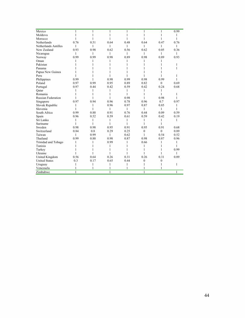
44
Mexico 1 1 1 1 1 1 0.99 Moldova 1 1 1 1 1 1 1 Morocco 1 1 1 1 1 1 1 Netherlands 0.76 0.51 0.64 0.48 0.64 0.47 0.76 Netherlands Antilles 1 1 1 1 1 1 1 New Zealand 0.93 0.98 0.62 0.56 0.62 0.05 0.36 Nicaragua 1 1 1 1 1 1 1 Norway 0.99 0.99 0.98 0.89 0.98 0.89 0.93 Oman 1 1 1 1 1 1 Pakistan 1 1 1 1 1 1 1 Panama 1 1 1 1 1 1 1 Papua New Guinea 1 1 1 1 1 1 Peru 1 1 1 1 1 1 1 Philippines 0.99 1 0.98 0.99 0.98 0.99 1 Poland 0.97 0.99 0.95 0.89 0.82 0 0.69 Portugal 0.97 0.44 0.42 0.59 0.42 0.24 0.68 Qatar 1 1 1 1 1 1 Romania 1 1 1 1 1 1 1 Russian Federation 1 1 1 0.98 1 0.98 1 Singapore 0.97 0.94 0.96 0.78 0.96 0.7 0.97 Slovak Republic 1 1 0.96 0.97 0.87 0.85 1 Slovenia 1 1 1 1 1 1 1 South Africa 0.99 0.88 0.91 0.76 0.44 0.09 0.59 Spain 0.96 0.52 0.59 0.61 0.59 0.42 0.19 Sri Lanka 1 1 1 1 1 1 1 Suriname 1 1 1 1 1 1 Sweden 0.98 0.98 0.95 0.91 0.95 0.91 0.68 Switzerland 0.84 0.8 0.29 0.25 0 0 0.89 Taiwan 1 0.99 1 0.62 1 0.54 0.52 Thailand 0.99 0.88 0.98 0.87 0.98 0.87 0.96 Trinidad and Tobago 1 1 0.99 1 0.66 1 1 Tunisia 1 1 1 1 1 1 1 Turkey 1 1 1 1 1 1 0.99 Ukraine 1 1 1 1 1 1 1 United Kingdom 0.56 0.64 0.26 0.31 0.26 0.31 0.89 United States 0.3 0.17 0.65 0.44 0 0 Uruguay 1 1 1 1 1 1 1 Venezuela 1 1 1 1 1 1 Zimbabwe 1 1 1 1

45
Tab
le A
2: O
rigi
nal S
in a
nd E
xcha
nge
Rat
e Fl
exib
ility
(1
) (2
) (3
) (4
) (5
) (6
) (7
) (8
) (9
) (1
0)
(11)
(1
2)
D
ropp
ing
Fina
ncia
l C
ente
rs
Dro
ppin
g Fi
nanc
ial
Cen
ters
D
ropp
ing
Fina
ncia
l C
ente
rs
LY
S LY
S LY
S LY
S R
ESM
2 R
ESM
2 R
ESM
2 R
ESM
2 R
VER
R
VER
R
VER
R
VER
O
SIN
2 1.
401
0.
230
0.
415
0.
733
-1
.820
-1.2
29
(1.8
3)*
(0
.24)
(3.5
4)**
*
(4.2
6)**
*
(3.0
4)**
*
(1.8
7)*
O
SIN
3
1.50
3
1.11
2
0.24
8
0.33
9
-0.8
01
-0
.598
(3
.56)
***
(2
.45)
**
(3
.74)
***
(3
.10)
***
(2
.02)
**
(1
.33)
LG
DP_
PC
0.14
3 0.
302
0.10
5 0.
285
-0.0
02
-0.0
53
0.00
5 -0
.052
-0
.093
0.
026
-0.0
78
0.02
5
(1.2
5)
(2.8
9)**
* (0
.93)
(2
.77)
***
(0.1
3)
(1.8
5)*
(0.2
7)
(1.8
1)*
(1.6
2)
(0.6
1)
(1.3
3)
(0.5
6)
OPE
N
0.09
4 0.
198
0.04
2 0.
153
0.04
9 -0
.014
0.
048
-0.0
14
0.74
3 1.
017
0.75
1 1.
021
(0
.43)
(0
.92)
(0
.20)
(0
.72)
(1
.15)
(0
.41)
(1
.13)
(0
.41)
(1
.98)
* (2
.88)
***
(1.9
9)*
(2.9
3)**
* SH
AR
E2
0.34
4 0.
290
0.35
1 0.
297
0.00
0 -0
.036
-0
.003
-0
.030
-0
.305
-0
.570
-0
.310
-0
.544
(1.8
6)*
(0.9
6)
(1.9
8)*
(0.9
8)
(0.0
0)
(0.6
6)
(0.0
8)
(0.5
4)
(1.8
2)*
(2.3
6)**
(1
.89)
* (2
.29)
**
Con
stan
t -0
.764
-2
.188
0.
710
-1.6
44
-0.1
32
0.53
1 -0
.503
0.
435
2.21
5 0.
104
1.51
3 -0
.084
(0.5
2)
(1.9
4)*
(0.4
4)
(1.4
6)
(0.5
4)
(1.7
3)*
(1.7
0)*
(1.3
5)
(2.6
4)**
(0
.17)
(1
.71)
* (0
.13)
O
bser
vatio
ns
75
75
71
71
65
65
62
62
65
65
62
62
R-s
quar
ed
0.18
0.
37
0.14
0.
34
0.52
0.
62
0.51
0.
65
Rob
ust t
stat
istic
s in
pare
nthe
ses
(Wei
ghte
d O
LS fo
r RES
M2
and
RV
ER, W
eigh
ted
Tobi
t for
LY
S)
*s
igni
fican
t at 1
0%; *
* si
gnifi
cant
at 5
%; *
** si
gnifi
cant
at 1
%

46
Tab
le A
3: O
rigi
nal S
in a
nd M
acro
econ
omic
Vol
atili
ty
(1
) (2
) (3
) (4
) (5
) (6
) (7
) (8
)
Dro
ppin
g Fi
nanc
ial C
ente
rs
Dro
ppin
g Fi
nanc
ial C
ente
rs
V
OL_
GR
OW
TH
VO
L_G
RO
WTH
V
OL_
GR
OW
TH
VO
L_G
RO
WTH
V
OL_
FLO
W
VO
L_FL
OW
V
OL_
FLO
W
VO
L_FL
OW
O
SIN
2 0.
016*
0.02
6
11.1
94
12
.937
(1
.68)
(2.1
0)**
(3.2
5)**
*
(2.7
8)**
OSI
N3
0.
011
0.
015
7.
103
7.
498
(1.9
6)*
(2
.45)
**
(3
.58)
***
(2
.69)
**
LGD
P_PC
-0
.006
-0
.012
-0
.006
-0
.012
-3
.191
-3
.214
-3
.242
-3
.322
(2.0
2)**
(2
.14)
**
(1.8
5)*
(2.0
9)**
(2
.69)
**
(2.5
6)**
(2
.38)
**
(2.4
0)**
O
PEN
0.
005
-0.0
01
0.00
5 -0
.000
-6
.320
-4
.181
-7
.062
-4
.333
(1.1
5)
(0.1
2)
(1.1
4)
(0.0
8)
(2.0
0)*
(1.2
0)
(1.5
8)
(0.8
3)
VO
L_TO
T -0
.000
-0
.000
-0
.000
-0
.000
0.
393
0.22
3 0.
382
0.22
3
(0.3
9)
(0.8
6)
(0.4
6)
(0.8
9)
(2.3
2)**
(1
.08)
(2
.18)
**
(1.0
2)
SHA
RE2
-0
.003
-0
.014
-0
.003
-0
.015
5.
074
0.14
7 5.
609
0.94
9
(1.1
4)
(1.7
2)*
(1.1
1)
(1.5
1)
(2.3
2)**
(0
.04)
(1
.70)
(0
.14)
C
onst
ant
0.07
0 0.
135
0.05
8 0.
131
26.4
78
32.8
25
25.7
58
33.2
82
(1
.88)
* (2
.25)
**
(1.4
3)
(2.1
5)**
(1
.97)
* (2
.39)
**
(1.5
7)
(2.2
2)**
O
bser
vatio
ns
77
77
73
73
33
33
29
29
R-s
quar
ed
0.21
0.
40
0.19
0.
40
0.65
0.
64
0.61
0.
62
Rob
ust t
stat
istic
s in
pare
nthe
ses
*
sign
ifica
nt a
t 10%
; **
sign
ifica
nt a
t 5%
; ***
sign
ifica
nt a
t 1%

47
Tab
le A
4: O
rigi
nal S
in a
nd C
redi
t Rat
ing
(1
) (2
) (3
) (4
) (5
) (6
) (7
) (8
) (9
) (1
0)
(11)
(1
2)
R
ATI
NG
1 R
ATI
NG
1 R
ATI
NG
1 R
ATI
NG
1 R
ATI
NG
1 R
ATI
NG
1 R
ATI
NG
1 R
ATI
NG
1 R
ATI
NG
1 R
ATI
NG
1 R
ATI
NG
1 R
ATI
NG
1
Dro
ppin
g Fi
nanc
ial C
ente
rs
OSI
N2
-15.
252
-12.
718
-9.4
97
-11.
078
-14.
487
-11.
874
(4
.35)
***
(3.7
8)**
*
(1
.70)
* (1
.81)
*
(4
.03)
***
(3.4
6)**
*
O
SIN
3
-5
.845
-5
.644
-5
.470
-4
.147
-5
.214
-4
.955
(4.0
8)**
* (4
.01)
***
(2.2
4)**
(1
.84)
*
(3
.31)
***
(3.2
1)**
* D
E_G
DP
-2.9
81
-2
.421
7.35
2
-1.8
37
-2
.969
-2.2
85
(3.2
2)**
*
(2.5
0)**
(0.9
1)
(0
.57)
(3.2
0)**
*
(2.3
2)**
DE_
RE
-0
.736
-0.9
99
0.
445
-0
.346
-0.7
75
-0
.975
(2
.14)
**
(2
.49)
**
(0
.12)
(0.3
7)
(2
.25)
**
(2
.39)
**
LGD
P_PC
2.
392
2.27
3 2.
916
2.67
0 2.
302
2.24
7 2.
906
2.62
1 2.
389
2.23
5 2.
976
2.72
9
(7.1
0)**
* (5
.63)
***
(8.4
8)**
* (6
.16)
***
(6.8
4)**
* (5
.48)
***
(8.3
6)**
* (5
.99)
***
(7.1
0)**
* (5
.54)
***
(8.3
6)**
* (5
.97)
***
DE_
GD
PSIN
2
-1
1.01
1
(1
.28)
DE_
RE_
SIN
2
-1.2
32
(0.3
2)
DE_
GD
PSIN
3
-0
.673
(0
.19)
DE_
RE_
SIN
3
-0.7
32
(0.7
7)
SHA
RE2
1.
501
1.58
9 2.
187
2.78
7 1.
569
1.59
7 2.
213
3.01
3 1.
518
1.65
6 1.
810
2.40
5
(2.6
6)**
(2
.36)
**
(1.4
3)
(1.5
2)
(2.8
3)**
* (2
.38)
**
(1.4
4)
(1.6
4)
(2.6
9)**
* (2
.47)
**
(1.0
9)
(1.1
8)
Con
stan
t 6.
174
4.72
3 -8
.058
-5
.962
1.
450
3.37
2 -8
.315
-6
.950
5.
435
4.24
8 -9
.119
-7
.037
(1.0
9)
(0.7
7)
(2.1
2)**
(1
.28)
(0
.22)
(0
.45)
(2
.06)
**
(1.4
5)
(0.9
5)
(0.6
9)
(2.2
9)**
(1
.44)
O
bser
vatio
ns
56
49
56
49
56
49
56
49
53
46
53
46
t sta
tistic
s in
pare
nthe
ses (
wei
ghte
d To
bit e
stim
atio
ns)
*
sign
ifica
nt a
t 10%
; **
sign
ifica
nt a
t 5%
; ***
sign
ifica
nt a
t 1%
48
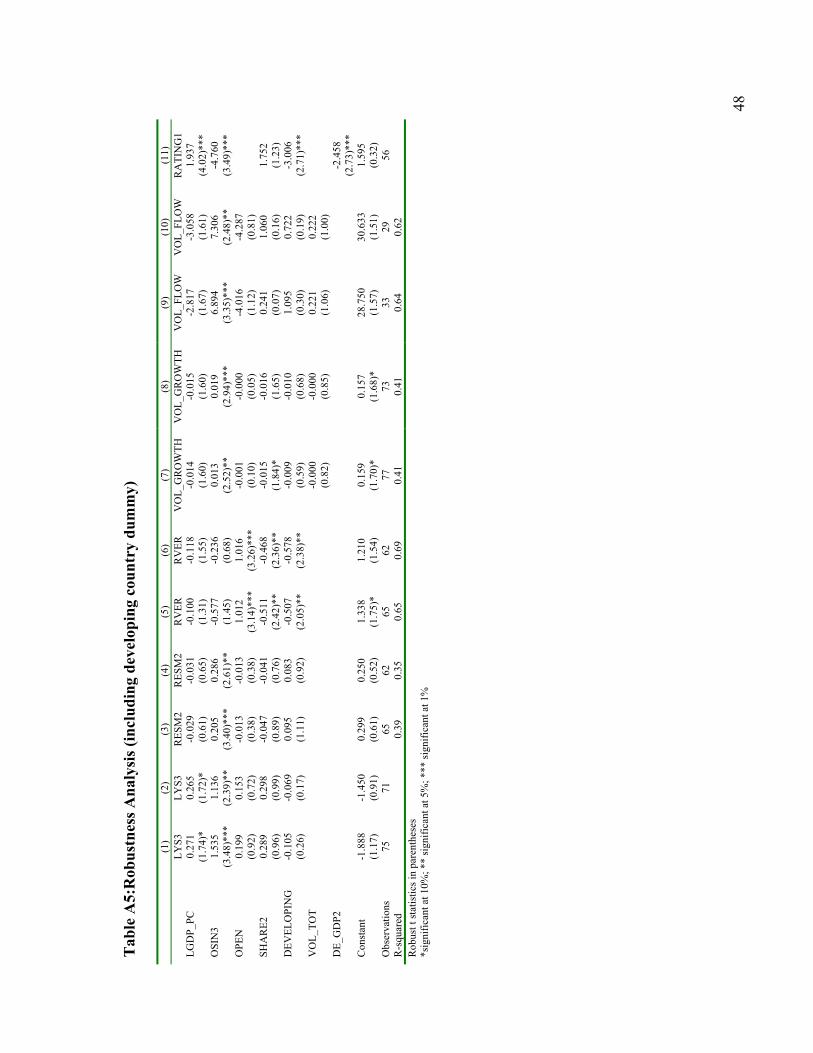
Tab
le A
5:R
obus
tnes
s Ana
lysi
s (in
clud
ing
deve
lopi
ng c
ount
ry d
umm
y)
(1
) (2
) (3
) (4
) (5
) (6
) (7
) (8
) (9
) (1
0)
(11)
LYS3
LY
S3
RES
M2
RES
M2
RV
ER
RV
ER
VO
L_G
RO
WTH
V
OL_
GR
OW
TH
VO
L_FL
OW
V
OL_
FLO
W
RA
TIN
G1
LGD
P_PC
0.
271
0.26
5 -0
.029
-0
.031
-0
.100
-0
.118
-0
.014
-0
.015
-2
.817
-3
.058
1.
937
(1
.74)
* (1
.72)
* (0
.61)
(0
.65)
(1
.31)
(1
.55)
(1
.60)
(1
.60)
(1
.67)
(1
.61)
(4
.02)
***
OSI
N3
1.53
5 1.
136
0.20
5 0.
286
-0.5
77
-0.2
36
0.01
3 0.
019
6.89
4 7.
306
-4.7
60
(3
.48)
***
(2.3
9)**
(3
.40)
***
(2.6
1)**
(1
.45)
(0
.68)
(2
.52)
**
(2.9
4)**
* (3
.35)
***
(2.4
8)**
(3
.49)
***
OPE
N
0.19
9 0.
153
-0.0
13
-0.0
13
1.01
2 1.
016
-0.0
01
-0.0
00
-4.0
16
-4.2
87
(0.9
2)
(0.7
2)
(0.3
8)
(0.3
8)
(3.1
4)**
* (3
.26)
***
(0.1
0)
(0.0
5)
(1.1
2)
(0.8
1)
SH
AR
E2
0.28
9 0.
298
-0.0
47
-0.0
41
-0.5
11
-0.4
68
-0.0
15
-0.0
16
0.24
1 1.
060
1.75
2
(0.9
6)
(0.9
9)
(0.8
9)
(0.7
6)
(2.4
2)**
(2
.36)
**
(1.8
4)*
(1.6
5)
(0.0
7)
(0.1
6)
(1.2
3)
DEV
ELO
PIN
G
-0.1
05
-0.0
69
0.09
5 0.
083
-0.5
07
-0.5
78
-0.0
09
-0.0
10
1.09
5 0.
722
-3.0
06
(0
.26)
(0
.17)
(1
.11)
(0
.92)
(2
.05)
**
(2.3
8)**
(0
.59)
(0
.68)
(0
.30)
(0
.19)
(2
.71)
***
VO
L_TO
T
-0
.000
-0
.000
0.
221
0.22
2
(0
.82)
(0
.85)
(1
.06)
(1
.00)
DE_
GD
P2
-2.4
58
(2
.73)
***
Con
stan
t -1
.888
-1
.450
0.
299
0.25
0 1.
338
1.21
0 0.
159
0.15
7 28
.750
30
.633
1.
595
(1
.17)
(0
.91)
(0
.61)
(0
.52)
(1
.75)
* (1
.54)
(1
.70)
* (1
.68)
* (1
.57)
(1
.51)
(0
.32)
O
bser
vatio
ns
75
71
65
62
65
62
77
73
33
29
56
R-s
quar
ed
0.39
0.
35
0.65
0.
69
0.41
0.
41
0.64
0.
62
R
obus
t t st
atis
tics i
n pa
rent
hese
s
*sig
nific
ant a
t 10%
; **
sign
ifica
nt a
t 5%
; ***
sign
ifica
nt a
t 1%
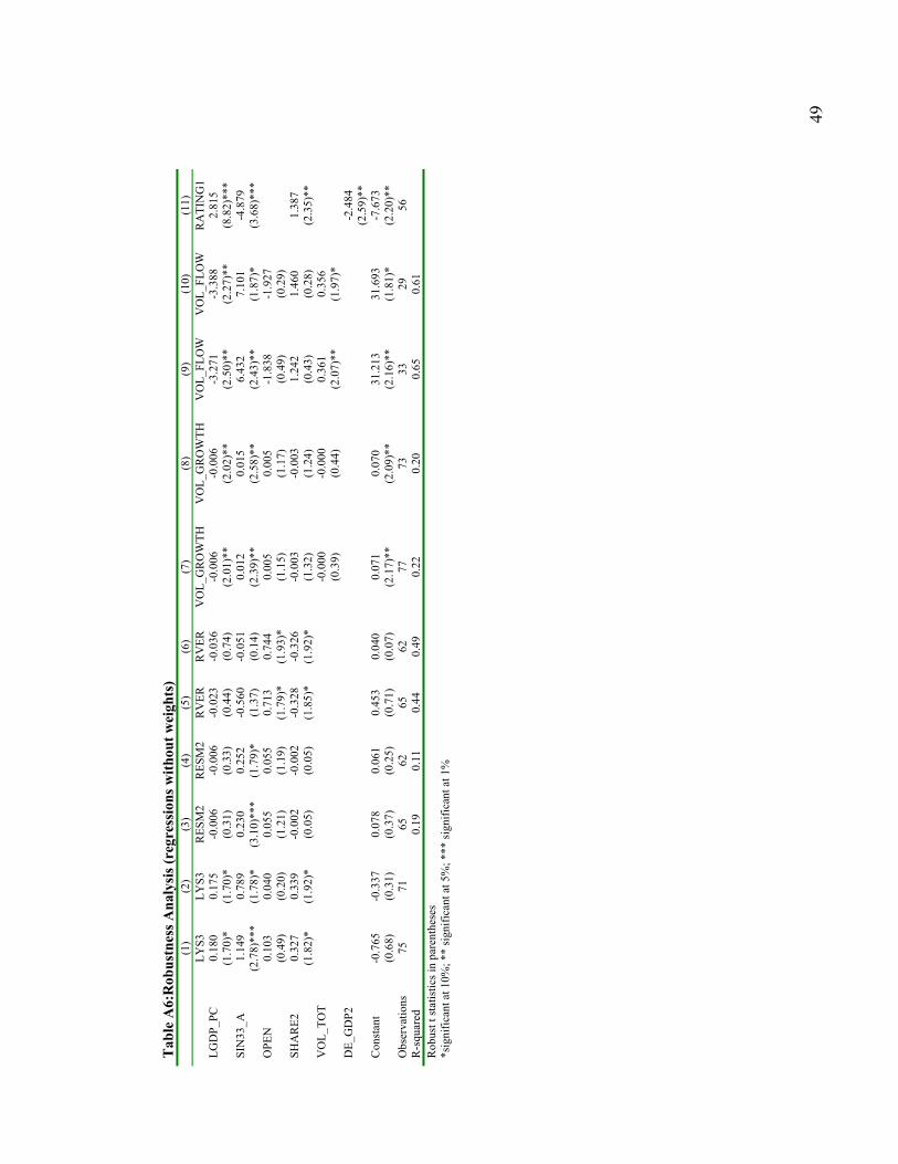
49
Tab
le A
6:R
obus
tnes
s Ana
lysi
s (re
gres
sion
s with
out w
eigh
ts)
(1
) (2
) (3
) (4
) (5
) (6
) (7
) (8
) (9
) (1
0)
(11)
LYS3
LY
S3
RES
M2
RES
M2
RV
ER
RV
ER
VO
L_G
RO
WTH
V
OL_
GR
OW
TH
VO
L_FL
OW
V
OL_
FLO
W
RA
TIN
G1
LGD
P_PC
0.
180
0.17
5 -0
.006
-0
.006
-0
.023
-0
.036
-0
.006
-0
.006
-3
.271
-3
.388
2.
815
(1
.70)
* (1
.70)
* (0
.31)
(0
.33)
(0
.44)
(0
.74)
(2
.01)
**
(2.0
2)**
(2
.50)
**
(2.2
7)**
(8
.82)
***
SIN
33_A
1.
149
0.78
9 0.
230
0.25
2 -0
.560
-0
.051
0.
012
0.01
5 6.
432
7.10
1 -4
.879
(2.7
8)**
* (1
.78)
* (3
.10)
***
(1.7
9)*
(1.3
7)
(0.1
4)
(2.3
9)**
(2
.58)
**
(2.4
3)**
(1
.87)
* (3
.68)
***
OPE
N
0.10
3 0.
040
0.05
5 0.
055
0.71
3 0.
744
0.00
5 0.
005
-1.8
38
-1.9
27
(0.4
9)
(0.2
0)
(1.2
1)
(1.1
9)
(1.7
9)*
(1.9
3)*
(1.1
5)
(1.1
7)
(0.4
9)
(0.2
9)
SH
AR
E2
0.32
7 0.
339
-0.0
02
-0.0
02
-0.3
28
-0.3
26
-0.0
03
-0.0
03
1.24
2 1.
460
1.38
7
(1.8
2)*
(1.9
2)*
(0.0
5)
(0.0
5)
(1.8
5)*
(1.9
2)*
(1.3
2)
(1.2
4)
(0.4
3)
(0.2
8)
(2.3
5)**
V
OL_
TOT
-0.0
00
-0.0
00
0.36
1 0.
356
(0.3
9)
(0.4
4)
(2.0
7)**
(1
.97)
*
DE_
GD
P2
-2.4
84
(2
.59)
**
Con
stan
t -0
.765
-0
.337
0.
078
0.06
1 0.
453
0.04
0 0.
071
0.07
0 31
.213
31
.693
-7
.673
(0.6
8)
(0.3
1)
(0.3
7)
(0.2
5)
(0.7
1)
(0.0
7)
(2.1
7)**
(2
.09)
**
(2.1
6)**
(1
.81)
* (2
.20)
**
Obs
erva
tions
75
71
65
62
65
62
77
73
33
29
56
R
-squ
ared
0.
19
0.11
0.
44
0.49
0.
22
0.20
0.
65
0.61
Rob
ust t
stat
istic
s in
pare
nthe
ses
*s
igni
fican
t at 1
0%; *
* si
gnifi
cant
at 5
%; *
** si
gnifi
cant
at 1
%


