THE IMPACT OF TEACHING MATHEMATICS WITH GEOGEBRA ON
THE CONCEPTUAL UNDERSTANDING OF LIMITS AND CONTINUITY:
THE CASE OF TURKISH GIFTED AND TALENTED STUDENTS
A MASTER’S THESIS
BY
MUSTAFA AYDOS
THE PROGRAM OF CURRICULUM AND INSTRUCTION
İHSAN DOĞRAMACI BILKENT UNIVERSITY
ANKARA
JUNE, 2015
MU
ST
AF
A A
YD
OS
2015


THE IMPACT OF TEACHING MATHEMATICS WITH GEOGEBRA ON THE
CONCEPTUAL UNDERSTANDING OF LIMITS AND CONTINUITY: THE
CASE OF TURKISH GIFTED AND TALENTED STUDENTS
The Graduate School of Education
of
İhsan Doğramacı Bilkent University
by
MUSTAFA AYDOS
In Partial Fulfilment of the Requirements for the Degree of
Master of Arts
The Program of Curriculum and Instruction
İhsan Doğramacı Bilkent University
Ankara
JUNE 2015

İHSAN DOĞRAMACI BILKENT UNIVERSITY
GRADUATE SCHOOL OF EDUCATION
The Impact of Teaching Mathematics with GeoGebra on the Conceptual
Understanding of Limits and Continuity: The Case of Turkish Gifted and Talented
Students
Mustafa Aydos
JUNE 2015
I certify that I have read this thesis and have found that it is fully adequate, in scope
and in quality, as a thesis for the degree of Master of Arts in Curriculum and
Instruction.
----------------------------
Assoc. Prof. Dr. M. Sencer Corlu (Supervisor)
I certify that I have read this thesis and have found that it is fully adequate, in scope
and in quality, as a thesis for the degree of Master of Arts in Curriculum and
Instruction.
----------------------------
Assoc. Prof. Dr. Serkan Özel
I certify that I have read this thesis and have found that it is fully adequate, in scope
and in quality, as a thesis for the degree of Master of Arts in Curriculum and
Instruction.
----------------------------
Assist. Prof. Dr. Jennie F. Lane
Approval of the Graduate School of Education
----------------------------
Prof. Dr. M. K. Sands (Director)

iii
ABSTRACT
THE IMPACT OF TEACHING MATHEMATICS WITH GEOGEBRA ON THE
CONCEPTUAL UNDERSTANDING OF LIMITS AND CONTINUITY: THE
CASE OF TURKISH GIFTED AND TALENTED STUDENTS
Mustafa Aydos
M.A., Program of Curriculum and Instruction
Supervisor: Assoc. Prof. Dr. M. Sencer Corlu
June, 2015
There is strong evidence in mathematics education literature that students benefit
extensively from the use of technology that allows for multiple representations of
mathematical concepts. The benefits include developing an advanced level of
mathematical thinking and conceptual understanding. The purpose of this study was
to investigate the impact of teaching limits and continuity topics in GeoGebra-
supported environment on students’ conceptual understanding and attitudes toward
learning mathematics through technology. The sample consisted of 34 students
studying in a unique high school for gifted and talented students in Turkey. This
study followed a pre-test post-test controlled group design. Conceptual
understanding of the topics of limits and continuity was measured through open-
ended questions while attitudes toward learning mathematics through technology
was measured using a Likert-type survey. The intervention was teaching with
GeoGebra in contrast to using traditional instruction in the control group. Data were
analyzed with an independent samples t-test on gain scores for control and

iv
experimental groups. In the conceptual understanding test, the gain scores of the
experimental group was found to be 1.33 standard deviations higher than that of the
control group on the average. This finding was evaluated noteworthy in terms of
previously-conducted research on the impact of GeoGebra. Furthermore, the study
found that student attitudes toward learning mathematics through technology
improved, as well. The researcher concluded that Geogebra may be an effective tool
for teaching calculus to gifted and talented students .
Keywords: limits and continuity concepts, dynamic geometry, computer algebra
systems, GeoGebra, technology integration in mathematics education, gifted and
talented students, affective domain, meta-analytical research.
v
ÖZET
MATEMATİĞİ GEOGEBRA İLE ÖĞRETMENİN LİMİT VE SÜREKLİLİK
KONULARININ KAVRAMSAL ANLAŞILMASINA OLAN ETKİSİ: ÜSTÜN
ZEKÂLI VE YETENEKLİ TÜRK ÖĞRENCİLERİ ÖRNEĞİ
Mustafa Aydos
Yüksek Lisans, Eğitim Programları ve Öğretim
Tez Yöneticisi: Doç. Dr. M. Sencer Çorlu
Haziran 2015
Matematik eğitimi literatüründe çoklu gösterime imkan sağlayan teknoloji
kullanımının, öğrencilerin ileri seviye matematiksel düşünme gücünü ve kavramsal
anlamalarını geliştirdiğine dair güçlü deliller vardır. Bu çalışmanın amacı, GeoGebra
yazılımı yardımı ile limit ve süreklilik öğretiminin kavramsal anlama ve matematiği
teknoloji ile öğrenme üzerine olan etkisini incelemektir. Çalışmanın örneklemi üstün
zekâlı ve özel yetenekli öğrencilerin bulunduğu bir okulda okuyan 34 lise
öğrencisidir. Ön ve son test kontrol gruplu araştırma deseni takip edilen bu
çalışmada, limit ve süreklilik konusundaki kavramsal anlama açık uçlu sorular ile
ölçülürken, matematiği teknoloji ile öğrenmeye karşı tutum Likert tipi anket ile
ölçülmüştür. Ders anlatımı deney grubunda GeoGebra yardımıyla, kontrol grubunda
ise geleneksel yöntemlerle yapılmıştır. Toplanılan data kontrol ve deney grubu ön ve
son test arasındaki fark (gelişme) puanları için bağımsız örneklem t testi ile analiz
edilmiştir. Deney grubunun fark kontrol grubuna nazaran 1,33 standart sapma daha
fazla gelişme gösterdiği görülmüştür. Bu sonuç daha önce yapılmış olan GeoGebra

vi
çalışmalarına göre kayda değer olarak değerlendirilmiştir. Ayrıca benzer bir gelişme
tutum ile ilgili sonuçlarda da görülmüştür. Sonuç olarak, analiz konularının
GeoGebra yardımıyla öğretilmesinin üstün zekâlı ve özel yetenekli öğrenciler
bağlamında etkili olabileceği düşünülmektedir.
Anahtar Kelimeler: limit ve süreklilik, dinamik geometri, bilgisayar cebir sistemleri,
GeoGebra, matematik eğitiminde teknoloji entegrasyonu, üstün zekâlı ve üstün
yetenekli öğrenciler, duyuşsal alan, meta-analiz.

vii
ACKNOWLEDGEMENTS
I would like to express my most sincere thanks to Prof. Dr. Ali Doğramacı and Prof.
Dr. Margaret K. Sands for their support that allowed me to study at Bilkent
University. I would also like to thank all other people at the Graduate School of
Education for their sincere support.
I would like to extend my deepest thanks to my adviser Assoc. Prof. Dr. M. Sencer
Corlu for constantly empowering and supporting me with his never ending patience
and lending me his assistance and experiences throughout the authoring process of
this thesis. I am very grateful for the time and energy spent by him for me. I am also
indebted to Asst. Prof. Dr. Jennie F. Lane and Assoc. Prof. Dr. Serkan Özel, who
participated in my dissertation defense as committee members, for their valuable
comments and special advice. I would like to thank Mr. Cecil Allen, Asst. Prof. Dr.
Jennie F. Lane, and Mr. Çağlar Özayrancı for helping me in the proofreading of my
thesis.
In addition, I would like to extend my special thanks to the administration and
teachers, particularly to my colleagues in the mathematics department, of the Turkish
Education Foundation, İnanç Türkeş Private High School for always supporting me
throughout my career.
Finally, I would like to express my most heartfelt thanks to my very dear father
ÖMER AYDOS, my very dear mother HAVAGÜL AYDOS, my beloved little sister
EDAGÜL AYDOS, and my precious wife KÜBRA KÖROĞLU AYDOS for their
infinite love, support, and encouragement. I would not have succeeded in this process
without them.

viii
TABLE OF CONTENTS
ABSTRACT……………………………………………………………………...
ÖZET………………………………………………………………………….....
ACKNOWLEDGEMENTS………………………………………………..….....
TABLE OF CONTENTS…...................................................................................
LIST OF TABLES…………………………………………………….................
LIST OF FIGURES……………………………………………………………...
CHAPTER 1: INTRODUCTION……………………………………………….
Introduction………………………………………………………………..
Background………………………………………………………………..
Problem……………………………………………………………….........
Purpose…………………………………………………………………….
Research questions………………………………………………………...
Significance………………………………………………………………..
Definition of key terms……………………………………………….........
CHAPTER 2: LITERATURE REVIEW………………………………………...
Introduction………………………………………………………………..
The multiple representation theory………………………………………...
Technology in mathematics education…………………………………….
Dynamic geometry software………………………………………...
GeoGebra……………………………………………………...
Research on teaching and learning calculus……………………………….
Limits and continuity concepts……………………………………...
Education for gifted and talented students…………………………….......
iii
v
vii
viii
xi
xiii
1
1
4
5
6
6
7
7
9
9
9
11
13
15
19
21
24

ix
CHAPTER 3: METHOD………………………………………………………...
Introduction………………………………………………………………..
Research design…………………………………………………………...
Pilot study………………………………………………………………....
The context and participants……………………………………………….
Data collection………………………………………………………….....
Procedure………………………………………………………….....
Instruments……………………………………………………..........
Limits and continuity readiness test…………………………..
Limits and continuity achievement test……………………….
Assessment criteria for LCRT and LCAT………………….....
The mathematics and technology attitudes scale……………...
Intervention………………………………………………………….
First and second lesson hours…………………………………
Third and fourth lesson hours…………………………………
Fifth and sixth lesson hours…………………………………...
Reliability and validity……………………………………………....
Data analysis……………………………………………………………….
CHAPTER 4: RESULTS………………………………………………………...
Conceptual understanding in limits and continuity……………………......
Impact at the question level……………………………………….....
Mann Whitney U test statistics………………………………..
Impact at the test level…………………………………………….....
Attitude towards technology in mathematics education……………….......
Impact at the item level……………………………………………...
26
26
26
28
29
32
32
32
32
33
34
34
35
36
40
45
52
54
57
57
57
60
63
66
66

x
Mann Whitney U test statistics………………………………..
Impact at the factor level………………………………………….....
Bivariate correlations between variables………………………………......
CHAPTER 5: DISCUSSION…………………………………………………….
Overview of the study……………………………………………………
Major findings…………………………………………………………......
Discussion of the major findings………………………………….....
Implications for practice…………………………………………………...
Implications for further research…………………………………………..
Limitations…………………………………………………………………
REFERENCES…………………………………………………………………...
APPENDICES…………………………………………………………………...
Appendix 1: Limits and continuity readiness test [LCRT]…………...........
Appendix 2: Limits and continuity avhievement test [LCAT]…………….
Appendix 3: Mathematics and technology attitude scale [MTAS]…..........
Appendix 4: Written permission for LCRT and LCAT……………….......
Appendix 5: Written permission for MTAS………………………….........
Appendix 6: Written permission of Ministry of National Education….......
Appendix 7: Worksheets……………………………………………..........
69
72
75
78
78
78
81
84
85
86
87
103
103
105
107
108
109
110
111

xi
LIST OF TABLES
Table Page
1 A summary of the research design 27
2 Gender distribution of participants 30
3 Participants’ primary school backgrounds 31
4 Parent occupations 31
5 Assessment criteria for LCRT and LCAT 34
6 Item total statistics of LCRT and LCAT scales 52
7 Item total statistics of MTAS pre-test and MTAS post-test
scales
53
8 Final Cronbach’s alpha values 54
9 Percent distribution of responses to each LCRT question 57
10 Percent distribution of responses to each LCAT question 58
11 Question level location statistics for each LCRT item 59
12 Question level location statistics for each LCAT item 60
13 The Mann-Whitney U test statistics between experimental
and control groups in each LCRT item
61
14 The Mann-Whitney U test statistics between experimental
and control groups in each LCAT item
62
15 Effect sizes in each LCAT item 63
16 Paired sample t-test statistics 64
17 Independent samples t-test statistics 64
18 Percent distribution of responses to each MTAS pre-test item 66
19 Percent distribution of responses to each MTAS post-test
item
67
20 Item level location statistics for each MTAS pre-test item 68
21 Item level location statistics for each MTAS post-test item 69

xii
22 The Mann-Whitney U test statistics between experimental
and control groups in each MTAS pre-test item
70
23 The Mann Whitney U test statistics between experiment and
control groups in each MTAS post-test item
71
24 Effect sizes in each MTAS post-test item 72
25 Independent t-test statistics for MTAS 73
26 Effect sizes in each MTAS domain 74
27 Bivariate correlations for control group (actual scores) 75
28 Bivariate correlations for experimental group (actual scores) 76
29 Bivariate correlations for control group (gain scores) 77
30 Bivariate correlations for experimental group (gain scores) 77
31 Overall effect size for GeoGebra’s impact with pre-test post-
test research
80

xiii
LIST OF FIGURES
Figure Page
1 GeoGebra applet for limiting (first function) 37
2 GeoGebra applet for limiting (second function) 37
3 GeoGebra applet for limiting (third function) 38
4 Table for algebraic calculations of the approaches 39
5 GeoGebra applet for investigating relations between circles
and polygons
41
6 GeoGebra applet for limiting (six different functions) 42
7 GeoGebra applet for explaining limit properties 43
8 Table for algebraic investigations of limit properties 43
9 A picture of a video for the circle area formula 44
10 GeoGebra applet for continuity 45
11 GeoGebra applet for investigation of the function y=1/x
around zero
46
12 GeoGebra applet for trigonometric limits and continuity 47
13 GeoGebra applet for investigation of the function y=sinx/x
around zero
48
14 A picture given as a clue to prove the limit of sinx/x around
zero
48
15 GeoGebra applet for continuity (twelve different functions) 50

1
CHAPTER 1: INTRODUCTION
Introduction
A widely-accepted learning theory in the psychology of mathematics education is
Bruner’s (1966) stages of representations or multiple representations theory (MR
theory). As a cognitive theory, Bruner’s approach to learning is action-oriented and
student-centered. Bruner’s theory characterizes three stages of representation:
enactive (representation through action), iconic (representation using visual images),
and symbolic (representation using symbols) (Goldin, 2014; Goldin & Kaput, 1996;
Tall, 1994). In mathematics education, “…representation refers both to process and
to product—in other words, to the act of capturing a mathematical concept or
relationships in some form and to the form itself…[including representations which
are] observable externally as well as those that occur ‘internally,’ in the minds of
people doing mathematics” (National Council of Teachers of Mathematics [NCTM],
2000, p. 67). Today, the MR theory is one of the most popular theories in
mathematics education and has dominated the field of mathematics education since
its introduction in 1960s during the new mathematics movement in the US.
Computer-algebra systems—CAS (see Artigue, 2002), dynamic geometry
software—DGS (see Clements, 2000), and graphing display calculators—GDC (see
Doerr & Zangor, 2000; Kastberg & Leatham, 2005) are some examples of modern
technological tools that enable students to think mathematically in a variety of
representations. There is strong evidence in mathematics education literature that, as
an application of the MR theory, students benefit extensively from the use of
2
technology in developing an advanced level of mathematical thinking and conceptual
understanding (Özgün-Koca & Meagher, 2012). The MR theory is believed to be
well-suited to explain the effective utilization of technology for conceptual
understanding in mathematics.
Effectively integrating technology into mathematics education has been
demonstrated through various software programs. Effectiveness in utilizing
technology in mathematics education has been shown to be related to its capacity to
allow for timely, efficient, and accurate transfer of external and internal
mathematical thinking among enactive, iconic, and symbolic representations of
mathematical concepts (Bulut & Bulut, 2011; Kabaca, Aktümen, Aksoy, & Bulut,
2010; Mainali & Key, 2012; NCTM, 2003). Research has provided educators with
strong evidence that effective use of technology has resulted in noteworthy gains in
conceptual understanding in a variety of mathematical topics, including:
(a) geometry; polygons, triangles, circles and Cartesian coordinates (Filiz,
2009; Gülseçen, Karataş, & Koçoğlu, 2012; İçel, 2011; Mulyono, 2010; Selçik &
Bilgici, 2011; Shadaan & Eu, 2013; Uzun, 2014);
(b) algebra; functions, parabolas, trigonometry and real life problems
(Aktümen & Bulut, 2013; Hutkemri & Zakaria 2012; Reis & Özdemir, 2010; Zengin,
2011; Zengin, Furkan & Kutluca, 2012); and
(c) calculus; limits and continuity, differentiation, and integration (Caligaris,
Schivo & Romiti, 2015; Kepçeoğlu, 2010; Kutluca & Zengin, 2011; Taş, 2010).
The American-based NCTM (2003) states that DGS has emerged in recent years as
an effective technological tool for visualizing abstract mathematical structures. The

3
rationale was that mathematics uses everyday words with different meanings in
different contexts (Mitchelmore & White, 2004) and DGS was successful in creating
opportunities that would link real life and abstract mathematical concepts in a variety
of contexts (Aktümen & Bulut, 2013; Saab, 2011). Based on the empirical evidence
in favor of and policy-makers’ support for the effectiveness of DGS in mathematics
education, several types of DGS have become popular for teaching mathematics in
both the United States and Turkey (Bakar, Tarmizi, Ayub, & Yunus, 2009; Güven &
Kosa, 2008; Jones, 2000). Software, which can be categorized as CAS, has been
recognized as another aide that allowed users to do computation with mathematical
symbols (Aktümen, Horzum, Yıldız, & Ceylan, 2011). There has been some research
evidence that supported this family of software for facilitating conceptual
understanding, as well (Güven, 2012; Heugl, 2001; Pierce, 2005). Today, DGS and
CAS are considered two of the most popular families of software that are used in
teaching mathematics for conceptual understanding.
The GeoGebra software is equipped with features of both DGS and CAS. This
particular software has established its place as a popular tool that can be used at all
levels from primary school to university (Akkaya, Tatar & Kagızmanlı, 2011;
Aktümen & Kabaca, 2012; Hohenwarter & Fuchs, 2004; Hohenwarter & Jones,
2007; Hohenwarter & Lavicza, 2007; Kutluca & Zengin, 2011). In addition to its
functionality at all levels, GeoGebra is freeware and available in 45 different
languages, including Turkish. GeoGebra, which is widely used to teach geometry,
algebra, and calculus is an example of the effective use of MR theory in the
classroom (Hohenwarter, Hohenwarter, Kreis, & Lavicza, 2008).

4
Background
During the last decade, several educational reforms have been introduced in Turkey.
The rationale behind these reforms was that Turkey needs to keep up with world-
class standards in mathematics and science education. The effective use of
technology for teaching mathematics has been particularly emphasized in curricular
documents in mathematics education (Ministry of National Education [MoNE],
2005; 2013). In the latest curricular changes of 2013, MoNE has particularly advised
mathematics teachers to use software, such as DGS, CAS, spreadsheets, GDC, smart
boards, and tablets. This advise has revealed the need for Turkish mathematics
teachers to learn how to use these programs and to learn how to use them effectively.
In the meantime, the physical conditions and infrastructure of the classrooms needed
to be improved and modernized. To this end, MoNE has developed and introduced
several large-scale projects, the most important of which being the Fatih project—
figuratively referring to the Conqueror title of Mehmet II (an Ottoman sultan who
reigned between 1451 and 1481) and which can literally be translated as an acronym
for Fırsatları Artırma ve Teknolojiyi İyileştirme Hareketi [movement to enhance
opportunities and improve technology].
The Fatih project has been being piloted since 2010 in over 50 schools located in 17
different provinces of Turkey. The ultimate goal of the project was to increase the
use of information and communication technologies (ICT) in the classroom; and
thus, provide equal access to technology in schools across Turkey. The project
website states the overall goal as that, “…42,000 schools and 570,000 classes will be
equipped with the latest information technologies and will be transformed into
computerized classes” (MoNE, 2012). In order accomplish this goal, there emerged a

5
need to educate mathematics teachers who are capable of employing these
technologies effectively. The first objective of the project was to provide smart
boards, projectors, internet access, copiers, and printers along with a tablet computer
for each student in every classroom in Turkey. The second objective was to deliver
in-service training (professional development) for teachers of all subject areas. By
ensuring the necessary physical conditions and through the delivery of extensive
training on subject-specific technology use, mathematics teachers were expected to
effectively integrate technology into their teaching.
Along with the support of the new curricula of 2013, the developments in
technological infrastructure of the schools, and professional development activities
for teachers, Fatih project is expected to create learning opportunities for students
who encounter difficulties in understanding abstract mathematical concepts.
Proceeding from this point, the need for affordable, user-friendly, and accessible
(i.e., availability in Turkish language) software has been critical for the success of
the project. As one of these software programs, GeoGebra is perceived by many as a
promising technology (Aktümen, Yıldız, Horzum, & Ceylan, 2011; Kabaca,
Aktümen, Aksoy, & Bulut, 2010; Tatar, Zengin, & Kağızmanlı, 2013).
Problem
First, despite the supporting evidence deducted from studies investigating the impact
of similar software programs with different populations of learners, including
students in Turkey (Almeqdadi, 2000; Bulut & Bulut, 2011; İpek & İspir, 2011;
Kabaca, 2006; Kepçeoğlu, 2010; Subramanian, 2005; Zengin, Furkan, & Kutluca,
2012), there is limited empirical research on the impact of these programs at the high
6
school level or that measures the impact on conceptual understanding in calculus
topics. Thus, there is a need to investigate the impact of GeoGebra on Turkish high
school students’ conceptual understanding of calculus topics.
Second, it is generally expected that around two percent of the individuals in the
society are gifted and talented (G&T) when measured through IQ tests (MoNE,
2009). Yet, the number of studies conducted for G&T student populations in terms of
teaching mathematics with technology is insufficient. Thus, there is a need to
investigate the impact of GeoGebra on Turkish G&T students’ conceptual
understanding in mathematics and particularly in calculus.
Purpose
The main purpose of this study was to investigate the impact of teaching
mathematics using the GeoGebra software on 12th grade G&T students' conceptual
understanding of limits and continuity concepts. A secondary purpose was to
investigate the impact of GeoGebra on students’ attitudes towards learning
mathematics with technology.
Research questions
The main research questions of the current study were:
a) What is the impact of using GeoGebra on G&T students’ conceptual
understanding of limits and continuity concepts?
b) What is the impact of using GeoGebra to teach limits and continuity concepts on
G&T students’ attitude towards learning mathematics with technology?
The null hypotheses can be stated as follows:

7
H0
where stands for the mean of experimental group’s gain scores,
and stands for the mean of control group’s gain scores. Gain scores are
the difference between post-test and pre-test scores. The null hypothesis (H0) states
that there is no statistically significant difference between the mean gain scores of
experimental and control groups. The alternative hypothesis (HA) states that there is a
statistically significant difference between the gain scores of experimental and
control groups on the average.
Significance
The use of technology has significantly increased in Turkey in recent years. These
developments have led to certain innovations and reforms in the field of education.
These innovations and reforms encourage both teachers and students to use
technology in the teaching and learning process. This study contributed to such
efforts that focus on increasing the quality and number of resources for students,
teachers, and curriculum developers, as well as providing them with empirical
evidence. It also serves as an example regarding investigations in other topics of
mathematics and leads the way to further research on gifted and talented students.
Definition of key terms
Multiple Representation (MR) theory emphasizes differentiation through
representations and states that there are three stages of cognitive processes, which are
enactive, iconic, and symbolic (Bruner, 1966).

8
Dynamic Geometry Software (DGS) refers to the family of software that
assists teachers and students to teach/learn the relations between geometrical
behaviors and shapes (Aktümen, Horzum, Yıldız, & Ceylan, 2011).
Computer Algebra System (CAS) refers to the family of software that allows
teachers and students to do symbolic and algebraic operations in mathematics in a
simpler and easier way (Kabaca, 2006).
Ministry of National Education (MoNE) is the state authority that regulates
and allows the opening of all educational institutions from the pre-school level to the
end of the 12th grade, that develops their curricula, and that incorporates all kinds of
services in education and training programs in Turkey.
GeoGebra is a free and user-friendly mathematics software, which includes
features of both DGS and CAS and has been translated into more than 40 languages.
The software can be used from the primary school to university level. “GeoGebra
brings together geometry, algebra, spreadsheets, graphing, statistics, and calculus”
(GeoGebra Tube, 2015).
Conceptual understanding is about making connections between previously
learned mathematical concepts and the concept which is being learned or the topics
which will be learned in the future. Students with a conceptual understanding are
assumed to be skilled in explaining concepts in depth.
Traditional instruction is assumed to be teacher centered where the teacher in
the control group in this study used still (non-dynamic) graphs or power-point
presentations. The instruction was mostly based on question-answer conversations
with the students or paper-pencil activities.

9
CHAPTER 2: LITERATURE REVIEW
Introduction
This chapter establishes the theoretical framework for the study. The purpose is to
present a synthesis of theory and research on multiple representations, the use of
technology in mathematics instruction and learning, and the role of dynamic
geometry software. Research on gifted and talented students in Turkey is included.
First, multiple representations (MR) theory is introduced as a constructivist theory of
mathematics education. Second, research on the use of dynamic geometry software
(DGS) and computer algebra systems (CAS) in mathematics education is critically
analyzed. Third, previous studies exploring issues relevant to the teaching and
learning of calculus (particularly limits and continuity) concepts are investigated.
Finally, a short summary of issues with regards to gifted and talented (G&T)
students’ education and related research is summarized.
The multiple representations theory
Jerome Bruner, a prominent psychologist, proposed several theories in the field of
education. Bruner’s theories focused on cognitive psychology, developmental
psychology, and educational psychology (Shore, 1997). Bruner’s approach to
learning was based on two modes of human thought: logico-scientific and narrative.
In order for these modes of thought to be effective, Bruner emphasized the notion
that learners would have a better understanding of abstract concepts if a
differentiated learning strategy was planned and implemented according to the
learner’s individual strengths (Bruner, 1985).

10
Bruner’s theory (1966), which emphasized differentiation through representations,
stated that there were three stages of each mode of thought: enactive, iconic, and
symbolic.
The enactive stage focused on physical actions: Learning happens through
movement or actions. Playing with a solid object and exploring its properties
is an example of the enactive stage. In a virtual environment (such as DGS or
GeoGebra), this stage is interpreted as manipulating the graphs by using
pointers (mouse) or hand-held computers.
The iconic stage fostered developing mental processes through vivid
visualizations: Learning happens through images and icons. Investigating the
properties of a solid shape from the text book images is an example of iconic
stage. In a virtual environment, this stage is interpreted as observing teacher
or peer demonstration on graphs or tables.
The symbolic stage was characterized by the storage metaphor where
information was kept in the form of codes or symbols: Learning happens
through abstract symbols. Finding out a solid’s surface area or volume by
using mathematical symbols is an example of symbolic stage. In a virtual
environment, this stage is interpreted as working with the symbolic equations.
Bruner’s work on representations has been interpreted as MR theory in mathematics
education. Many believed that MR theory would offer an explanation how students
learn abstract mathematical concepts through a variety of mathematical
representations (Cobb, Yackel, & Wood, 1992; Duval, 2006; Goldin, 2008), and that
view was agreed upon by several other reformist mathematics educators (e.g.,
Brenner et al., 1997) along with some influential mathematics education

11
organizations (e.g., National Council of Teachers of Mathematics [NCTM], 2000).
Some prominent researchers advocated for MR theory due its ability to support
students’ cognitive processes in authentic, real-life problems and learning
environments (e.g., Schonfeld, 1985). Some researchers proposed that learning
environments that foster conceptual understanding through MR theory could be best
created through the use of technology. According to these mathematics educators,
technology offered several opportunities for students to learn abstract concepts in
ways that are customized and based on students’ individual learning styles and
interests (Alacaci & McDonald, 2012, Kaput & Thompson, 1994; Özgün-Koca,1998,
2012). Some other researchers advocated for the use of the MR theory to establish
the missing link between technology and mathematics education (Gagatsis & Elia,
2004; Özmantar, Akkoç, Bingölbali, Demir, & Ergene, 2010; Panasuk &
Beyranevand, 2010; Pape & Tchoshanov, 2001; Swan, 2008; Wood, 2006). Today,
there is a consensus among mathematics educators that MR theory is an integral part
of reformist mathematics education and that technology plays an important role in
achieving the desired outcomes of the reforms.
Technology in mathematics education
Technology has been playing an increasingly important role in fostering conceptual
understanding in mathematics education (Özel, Yetkiner & Capraro, 2008).
According to the NCTM (2000), the use of technology has been an essential tool for
teaching and learning mathematics at all grade levels as it improves student skills in
decision making, reasoning, and problem solving. Similarly, several mathematics
educators believe that teaching mathematics in technologically-rich environments

12
was more effective than using paper-pencil based teaching methods (Clements, 2000;
Schacter, 1999; Vanatta & Fordham, 2004).
Policy makers in Turkey have been encouraging teachers to integrate technology into
mathematics classrooms. The Scientific and Technological Research Council of
Turkey (TÜBİTAK, 2005) indicated that teachers at all levels needed to utilize new
technologies into their teaching. Related to this point of view, TÜBITAK-initiated
Vision 2023 document emphasized the smart use of technology in education
(TÜBİTAK, 2005). In addition, The Ministry of National Education (MoNE, 2013)
encouraged Turkish mathematics teachers to teach students the skills required to
actively use information and communication technologies (ICT) in mathematics.
In accordance with the ideas proposed by influential policy making organizations,
some research in the Turkish context supported the use of technology in mathematics
education. For example, Baki (2001) argued that teachers could use innovative
computer technologies not only for teaching content but also to help students learn
mathematics by themselves. In another study, Baki and Güveli (2008) indicated that
teachers could increase student success through creating well-prepared,
technologically-rich learning environments. Bulut and Bulut (2011) found that
Turkish mathematics teachers were open to adapting a variety of technologically-rich
teaching methods when they believed that these methods would assist students to
understand abstract concepts. Çatma and Corlu (2015); however, showed that
Turkish mathematics teachers teaching high-ability students at specizalized schools
were not more mentally prepared to implement Fatih project technologies than
teachers at non-selective general schools.

13
Dynamic geometry software
The family of software that can be categorized as DGS has been considered by many
as one of the most effective technological tools to foster conceptual understanding in
mathematics education. Several researchers supported this view, claiming that such
software would help students benefit from multiple representations of mathematical
topics (Akkaya, Tatar, & Kağızmanlı, 2011; Hohenwarter & Fuchs, 2004; Kabaca,
2006; Zengin, Furkan, & Kutluca, 2012). The research of Kortenkamp (1999)
encouraged instructors to use DGS in their teaching because of its capacity to foster
understanding of multiple topics of advanced mathematics at both school and
university levels, including different geometries, such as the Euclidean, linear space,
and projective geometries, complex tracing and algebra, such as matrices, functions,
limits, and continuity. Kortenkamp advocated that students who used DGS could
explore multiple perspectives in a single construction.
Another evidence in favor of DGS was based on research that investigated the impact
of DGS for developing mathematical skills exclusively at the school level. For
example, Jones (2001) conducted a study to investigate the impact of DGS in
learning geometry concepts. The researcher’s sample included lower-secondary
students (12 year olds). The findings showed that using DGS in mathematics classes
had positive impacts on learning geometry concepts.
In another study, Subramanian (2005) investigated the impact of DGS on students’
logical thinking skills, proof construction, and general performances in their
mathematics courses. With a large sample of 1,325 high school students drawn from
local schools in the United States, the researcher used a double pre-post test design to

14
conclude that academically high achieving students benefited the most from using
DGS in developing logical thinking skills.
In an empirical study by Bakar, Tarmizi, Ayub, and Yunus (2009), however, no
statistically significant difference was reported for either conceptual understanding or
procedural knowledge in quadratic functions between a control group taught with a
traditional approach and a treatment group taught with DGS, in terms of student
performance after an intervention with DGS. Researchers believed that their
intervention, which was limited to six hours of instruction including the time spent to
learn basic features of the DGS in the experimental group, needed to be longer for an
impact to be observed.
Karakuş (2008) investigated student achievement in transformation geometry when
DGS was used as the medium of instruction. The researcher conducted the study
with 90 seventh-grade students in a school from Turkey. The research design
included a pre-test and a post-test. Karakuş divided the students into four groups
according to their pre-test scores (high-success experimental and control groups;
low-success experimental and control groups). After the intervention, there was a
statistically significant difference between the high-success experimental and the
control groups, in favor of the group of students who were taught with DGS, while
there was not a statistically significant difference between the low-success
experimental and the control groups. This research was noteworthy because it
showed that DGS might be an effective tool for high-success students with a large
impact of 1.31 standard deviations.

15
İpek and İspir (2011) believed that DGS was essential both for students and teachers
because such software brings about an environment that enables discourse and
exploration. The researchers examined pre-service elementary mathematics teachers’
algebraic proof processes and attitudes towards using DGS while making algebraic
proofs. They designed a ten-week long course. The participants solved problems
about algebra and proved some elementary theorems. The participants also wrote
their reflections. At the end of the course, researchers interviewed a selected number
of participants about their experiences with DGS. They found some pre-service
elementary mathematics teachers believed that DGS was valuable for learning and
teaching mathematics. Moreover, these informants reported a positive change in their
feelings for using technology.
In their study, Bulut and Bulut (2011) showed that the DGS allowed teachers to
observe and experience multiple teaching strategies. The purpose of their research
was to investigate pre-service mathematics teachers’ opinions about using DGS.
They followed a qualitative research methodology with some forty-seven students at
their sophomore year who reported a willingness to use DGS when they would
become teachers.
GeoGebra
GeoGebra is a freely-available and open-source interactive geometry, algebra and
calculus application created by Markus Hohenwarter in 2002. Hohenwarter and
Jones (2007) believe that GeoGebra is a useful tool for visualizing mathematical
concepts from the elementary to the university level. They emphasize that Geogebra
integrates two prominent forms of technology; namely, CAS and DGS. GeoGebra,

16
which offers dynamically connected multiple illustrations of mathematical objects
through its graphical, algebraic, and spreadsheet views, also allows students to
investigate the behaviors of the parameters of a function through its CAS component
(Hohenwarter & Lavicza, 2009). The software is constantly being improved by an
active team of researchers and teachers. The software has a large collection of
activities which are developed and donated by users all over the world. In recent
years, the software is being translated into a number of languages, making it
available in 45 different languages as of 2015.
Some researchers have explored the impact of GeoGebra on achievement of
objectives in different mathematical topics. Saha, Ayub, and Tarmizi (2010) used a
quasi-experimental post-test only design to identify the differences on the average for
high visual-spatial ability and low visual-spatial ability students after using
GeoGebra for learning coordinate geometry. In their study, the sample consisted of
53 students who were 16 or 17 years old from a school in Malaysia. The researchers
divided the sample into two homogeneous groups, where the experimental group
students were taught with GeoGebra and the control group students were taught with
traditional methods. Each group was categorized into two types of visual-spatial
ability (high [HV] and low [LV]) by applying a paper and pencil test covering 29
items. They reported three main findings:
(a) students in the experimental group scored statistically significantly higher
on the average than the students in the control group regardless of being HV or LV;
(b) in the HV group, there was no statistically significant difference on the
average between experimental and control groups in favor of the experimental group;
17
(c) in the LV group, students in the experimental group scored statistically
significantly higher on the average than the students in the control group.
This research was noteworthy because it showed that GeoGebra might be an
effective tool for LV students, as well.
Another research study reflecting the positive impact of GeoGebra was conducted by
Kllogjeri and Kllogjeri (2011) in Albania. The researchers presented some examples
of how GeoGebra was used to teach the concepts of derivatives. In the study, they
demonstrated three important theorems by using GeoGebra applets to explain: (a) the
first derivative test and the theorem; (b) the extreme value theorem; and (c) the mean
value theorem. The researchers used direct teaching method and measured
GeoGebra’s impact on students’ conceptual understanding. They concluded that the
multiple representation opportunities and the dynamic features of GeoGebra helped
students’ understand the mathematical concepts faster and at a deeper level.
Mehanovic (2011) wrote about GeoGebra that included two separate studies focusing
on teaching integral calculus with GeoGebra. The first study was conducted with
two classes from two different secondary school students in Sweden. The researcher
observed students through regular classroom visits. After several classroom
observations, individual interviews with students were conducted. For the second
study, the researcher asked the participating teachers to prepare an introduction to the
concept of integration and record their introductory presentations. The objective of
the study was to investigate teachers’ introductions to the subject of integrals in a
normal classroom environment. After the preliminary analysis of the teacher
presentations, individual interviews were conducted with the participating teachers.
As a result of the first study, it was found that the students had some concerns, such

18
as using GeoGebra was time-consuming. Furthermore, students seemed to believe
that using GeoGebra was more confusing than their previous learning methods. In
the second study, teachers reported some epistemological, technical, and didactical
barriers for effective use of GeoGebra in the classroom. However, it was concluded
in both studies that integrating a didactical environment with GeoGebra was complex
and teachers needed to realize the potential challenges.
Some GeoGebra impact studies were conducted in Turkey, as well. For example,
Selçik and Bilgici (2011) focused on the initial impact and the degree of retention of
knowledge for polygons. The study was conducted with 32 seventh-grade students.
Following a pre-test, the experimental group was instructed using GeoGebra and a
constructivist face-to-face teaching was provided to the control group that did not
have computer access. In the experimental group, one computer was given to every
two students to create a collaborative environment and that enabled students to
directly examine the prepared activities. Following an 11-hour long course, an
identical post-test was applied. Students in the experimental group scored higher
averages on the post-test than the students in the control group. When the test was
administered for the third time a month after the intervention ended, the students in
the experimental group performed better in terms of the amount of knowledge they
retained.
Similarly, Zengin (2011) conducted a study with 51 high-school students to
investigate the effect of the GeoGebra software in teaching the subject of
trigonometry and to examine students’ attitude toward mathematics. In this study,
participants were divided into two equal groups, one experimental and one control.

19
Both groups were given a pre-test. While teaching was focused on using the
GeoGebra software in the experimental group, the control group was taught with a
constructivist teaching approach only. Both groups showed improvement in their
achievement scores at the end of the study; although, the averages in the
experimental group were statistically significantly higher when compared with those
in the control group. However, according to the experimental groups’ pre- and post-
test scores, teaching mathematics through technology had negligible effect on
students’ attitudes toward mathematics.
A detailed analysis of effect sizes in selected and relevant impact studies is
summarized in Table 31.
Research on teaching and learning calculus
Calculus is a branch of mathematics that focuses on change. Calculus is taught both
in high school as an advance mathematics course or at university level as a freshman
(i.e., first year) course. Kidron (2014) stated that a usual calculus course consists of a
combination of several topics including limits, differentiation, and integration, in
which students are reported to experience difficulties in understanding. Students find
calculus topics difficult because it includes abstract definitions and formal proofs
(Tall, 1993).
Kidron (2014) asserted that the use of technology is one of the effective methods in
teaching calculus. Hohenwarter, Hohenwarter, Kreis and Lavicza (2008) advocated
that GeoGebra was a convenient software program for technology-supported
mathematics (particularly calculus) teaching and argued that calculus education using

20
GeoGebra could be applied to courses in two ways: (a) presentation (teacher-
centered approach); and (b) mathematical experiments (student-centered approach).
Tall, Smith and Piez (2008) examined 40 graduate-level theses on this topic authored
between 1998 and 2008. They concluded that most of the studied technologies
showed positive contribution to learning of calculus topics.
Several studies about teaching calculus have also been conducted in Turkey. Kabaca
(2006) instructed the limits topic using technology and traditional methods to
freshman mathematics students (n = 30). Dividing the sample into two as the control
(the group using traditional methods) and experimental (the group using
technological aids) groups and comparing the pre-test and post-test achievement
scores, the researcher did not find a statistically statistical difference on the average
between the group scores.
Aktümen and Kaçar (2008) instructed the concept of definite integral using
technology to first year university students of a science education department (n =
47). In their conclusion they stated that there was a statistically significant positive
improvement in the attitudes of the students in the class where technology was used
compared to the class where technology was not used.
Despite the growing knowledge-base, there is still a limited number of studies on
calculus teaching conducted at the high school level.

21
Limits and continuity concepts
Limits and continuity, which are the first steps to the subject of derivatives, are of
great importance in such fields as engineering and architecture. Both topics are
abstract concepts that confuse students when they first encounter them. In the new
mathematics curriculum of 2013, MoNE encourages the use of certain DGS that may
make such abstract topics accessible to students. MoNE prescribes 118 periods (of 40
minutes each) be dedicated to calculus in grade 12 (which is 54% of all the time
assigned for all topics). Of these 118 periods, the national curriculum advised that 14
classroom periods be allocated to teach about limits and continuity concepts, this
comprises 6% of the total contact hours in grade 12 mathematics (MoNE, 2013).
Because limits and continuity are abstract concepts that are difficult for teachers to
instruct and students to comprehend, various studies on the limits topic exist in the
literature. For example, Mastorides and Zachariades (2004) conducted a study to
understand the content knowledge of secondary mathematics teachers about the
concepts of limits and continuity. Fifteen secondary mathematics teachers, all
attending master’s degree programs in mathematics education, were enrolled in the
study. They taught calculus, particularly limits and continuity concepts, for 12 weeks
during their master’s degree program and the researchers noted their challenges. At
the end of the teaching period, participants were given a survey consisting of
questions about the problems they had to overcome during the intervention. After the
survey, the researchers conducted interviews with all the teachers. As a result, the
researchers argued that the participating teachers had the greatest concern regarding
their pedagogical content knowledge about the concepts of limits and continuity.

22
Another study about the limits concept was conducted by Blaisdell (2012) to
investigate how students’ answers change in terms of question and presentation
format in the limits concept. The researcher applied a test to 111 calculus students at
a university. The test questions focused on multiple representations such as graphs,
mathematical notations, and definitions in the limits concept. The study indicated
that students did best when the questions on limits were represented in graphs.
In Turkey, there are some similar studies focused on teaching and learning limits and
continuity concepts. Baştürk and Dönmez (2011) conducted a study to understand
pre-service mathematics teachers’ knowledge of different teaching methods and
representations of the limits and continuity topics. They gathered data from 37 pre-
service high-school mathematics pre-service teachers from a public university in
Turkey. In their research, the researchers used multiple research strategies to collect
data such as observation, interviews, and document analysis. The survey consisted of
questions to understand students’ content knowledge related to the limits and
continuity concepts.The researchers selected four students out of the 37 according to
their responses to conduct interviews, microteaching observations, and document
analysis. The interviews focused on about the teaching strategies for limits and
continuity before they were requested to make a lesson plan and to teach in the form
of microteaching. Although the students were aware that teachers should have made
the concept of limits and continuity more concrete using teaching strategies such as
drawing appropriate graphs or using technological devices, they all used question-
answer methods in their microteachings and documentation. Researchers concluded
that pre-service teachers should be encouraged to integrate innovative teaching
methods and use them to concretize such abstract concepts such as limits and
continuity.

23
Another study was conducted by Kabaca (2006) to understand the effect of CAS on
teaching limits. In his PhD dissertation, Kabaca used an experimental design to
examine a particular CAS named Maple while teaching limits to 30 pre-service
mathematics teachers. Kabaca aimed to investigate whether teaching with Maple had
any impact on student attitudes towards mathematics. The researcher divided
students into experimental and control groups based on their scores of pre-attitude
and pre-test on readiness for the limits concept. Then, Kabaca taught the limits
concept in a 28 hour-course to the control group with a constructivist teaching
method and to the experimental group with CAS-assisted constructivist approach.
After the intervention, the post-test and post-attitude data were analyzed. In
conclusion, the researcher deducted three major results comparing post test data for
control and experimental groups:
(a) teaching with CAS had no statistically significant effect on students’ total
post-test score;
(b) teaching with CAS had a statistically significant effect on students’
conceptual understanding of limits and continuity at the post-test level but no
statistically significant difference was observed for procedural knowledge or problem
solving skills;
(c) teaching with CAS had statistically significant positive effect on students’
attitude towards mathematics.
Kepçeoğlu (2010) studied the effect of GeoGebra on students’ achievement and
conceptual understanding of the concepts of limits and continuity. Similarly, he
designed an experimental study to conduct a study with 40 second-year pre-service
elementary mathematics teachers. Kepçeoğlu divided the students into two groups

24
(experimental and control) based on their pre-test scores. Researcher taught the limits
and continuity concepts for a duration of six-lesson hours using traditional teaching
methods to the control group, and using instructional methods along with GeoGebra
to the experimental group. After the intervention, the researcher applied the same test
as post-test to both groups; and compared the scores gathered from the pre- and post-
tests. Kepçeoğlu concluded that teaching the limits concept to pre-service elementary
mathematics teachers within the GeoGebra environment was more effective than the
traditional teaching methods in terms of students’ conceptual understanding.
Although GeoGebra had a similar contribution in teaching the continuity concept, the
effect was smaller compared to its impact on limits.
Education for gifted and talented students
Individuals who are categorized as G&T are considered creative and productive
people. They are assumed to learn faster compared to their peers and to have multiple
interests (Karakuş, 2010). Identifying these individuals at an early age, providing
them with appropriate developmental opportunities, and leading them to suitable
careers are important. While measuring the level of intelligent quotient (IQ) was
considered adequate to identify intellectual giftedness until 30-35 years ago; today,
certain other tests (such as Progressive Matrices Test and performance evaluations)
are used along with the tests that measure the IQ level (Bildiren & Uzun, 2007).
Turkey’s experience with G&T individuals has a long history since the Enderun,
world’s first institution established for gifted and talented students during the 15th
century in İstanbul (Corlu, Burlbaw, Capraro, Han, & Corlu, 2010). More recently,
the Centers for Science and Art (Bilim ve Sanat Merkezleri—BİLSEM) were
25
established to identify talented G&T students in Turkey. Working in close
cooperation with schools around the country, BİLSEM has been instrumental in
identifying talented G&T students and creating enriched learning environments
appropriate for them. In addition, the Turkish Education Foundation has been
operating the first and still the only school for such students in modern Turkey since
1993.
Preparing enriched and in-depth lessons that promote critical thinking and creativity
in educating G&T students is one of the primary tasks of the teachers of G&T
students. A tool that teachers can use in planning and preparation for this purpose is
technology. In mathematics education, G&T students can be supported by
technology, based on their areas of interest and mathematical abilities (Hohenwarter,
Hohenwarter & Lavicza, 2010). In this regard, there are a few studies on G&T
students’ learning mathematics using technological aids. In their study conducted
with gifted students, Duda, Ogolnoksztalcacych, and Poland (2010) stated that the
use of graphing display calculators helped students produce creative solutions and
provide them with opportunities to explore new mathematical concepts. Choi (2010)
specified that GeoGebra increased interest in and motivation toward mathematics.
Software programs that create environments of thinking creatively for G&T students
direct students to explore and produce authentic mathematical knowledge.

26
CHAPTER 3: METHOD
Introduction
The main purpose of this study was to investigate the impact of teaching
mathematics with GeoGebra on 12th grade gifted and talented (G&T) students'
conceptual understanding of the limits and continuity concepts. The second purpose
was to investigate the impact of GeoGebra on students’ attitudes towards learning
mathematics with technology. This chapter discusses the research design, pilot study,
participants, instruments used in data collection, and data analysis.
Research design
A pre-post test design was employed in the study to determine the impact of teaching
with GeoGebra software on conceptual understanding of G&T students and their
attitudes towards learning mathematics with technology. The participants of the
study had already been divided into two classes by the school administration before
the study—later determined randomly as an experimental group and a control group
by the researcher. In this manner, the assignment of participants into the groups was
not manipulated by the researcher. In order to correct for any possible difference in
their ability and knowledge before the intervention, both groups were administered
the limits and continuity readiness test (LCRT) along with the mathematics and
technology attitude scale (MTAS). Following the pre-test, the limits and continuity
concepts were taught to the experimental group in the GeoGebra environment;
whereas the same concepts were taught with the traditional direct instruction
methods to the control group. With the conclusion of the teaching process in two

27
weeks, the limits and continuity achievement test (LCAT), a test closely similar to
LCRT, was applied and the same attitude survey that was administered in the pre-test
stage were given as a post-test. The research design is summarized in Table 1.
Table 1
A summary of the research design
Group Pre-tests Intervention Post-tests
Experimental Group LCRT
MTAS
Teaching with
GeoGebra
LCAT
MTAS
Control Group LCRT
MTAS
Teaching with
traditional method
LCAT
MTAS
In quantitative research, the researcher states a hypothesis, tests this hypothesis, and
generalizes the results to a larger population (Arghode, 2012). Huck (2011) stated a
nine-step version of hypothesis testing which was followed in the current study:
(1) State the null hypothesis,
(2) State the alternative hypothesis,
(3) Specify the desired level of significance,
(4) Specify the minimally important effect size,
(5) Specify the desired level of effect size,
(6) Determine the proper size of sample,
(7) Collect and analyze the sample data,
(8) Refer to a criterion for assessing the sample evidence,
(9) Make a decision to discard/retain.

28
Pilot study
Before the actual data collection, a pilot study with 12th grade high-school students
of a private high-school in Ankara was conducted. The goals of this pilot study
included the following:
(a) finalize the research questions and research design before the actual study
with G&T students;
(b) review of the data collection process before the study;
(c) identification of possible problems that can be encountered during the
course of the study;
(d) determination of the appropriate sample size for the study;
(e) identification of the shortcomings of data collection instruments and
elimination of these shortcomings (Orimogunje, 2011).
The pilot study was conducted with a group of 26 students. The group was already
divided into two sub-groups (the experimental and control groups) by the school
administration. The experimental group was provided with the limits and continuity
instruction (intervention) using GeoGebra whereas the control group was taught the
same topic with traditional method by the same teacher. The instruction period was
limited to 2 weeks (10 hours). Following the instruction, the limits and continuity
post-test was applied.
The pilot revealed problems experienced during the intervention process. The
researcher made the following arrangements and changes to ensure that the study
would yield reliable data:

29
(a) The sample size was estimated through a prior power analysis with
G*Power3;
(b) the procedures and duration of the intervention were considered
appropriate for the main research upon feedback of school teachers and students;
(c) 12th grade students who were busy preparing for the university entrance
exams during the course of the research could not attend intervention classes
regularly. Given the fact that participants in the actual study were boarding students,
this was not considered a serious concern.
One of the biggest outcomes of conducting a pilot study was to calculate the required
sample size for the study (Teijlingen & Hundley, 2001). To calculate the required
sample size, a special software named G*Power3 was used. Based on pilot data, the
program estimated the effect size—strength of a relationship: Cohen’s d = 1.27 in
post test score differences between two groups. The magnitude of this effect, as well
as effect sizes reported in similar studies on GeoGebra was used as a benchmark for
meta-analytical purposes when assessing the effect of the intervention of the present
study (See Table 31). Thus, it was estimated that the required sample size needed to
be at least 22 in order to be 80% sure at an alpha level of .05 that there would be a
statistically significant difference between the experimental and control group scores
on the average.
The context and participants
This study was conducted with 34 students in grade 12 of a private high school in
Kocaeli, Turkey. This high school (grades 9 to 12) was founded to educate G&T
students who were selected on merit from all over Turkey. This unique school

30
established its vision as follows: To develop G&Tstudents who are suffering from
economic and social difficulties; to offer them a proper learning environment; and to
educate them as leaders of the society. In this sense, the participating students could
be described as strong individuals in terms of both academic and social aspects.
Because the school was a boarding school, students were staying in the school during
the weekdays. The school followed the International Baccalaureate (IB) Diploma
Programme (DP) in grade 11 and 12.
The school selects its students with several screening methods such as progressive
matrices test, WISC-R’s IQ test, interviews, and an observation camp that lasts for
one week, all administered at the end of 8th grade. Some of the students are admitted
with a full scholarship while others are provided with a partial scholarship.
According to the school regulations, 30% of the students should have full
scholarship, and the rest of the students get partial scholarship with respect to their
parents’ economic condition. The participating students of the current study reflected
the school scholarship ratios. See Table 2 for gender distribution of the participant
students.
Table 2
Gender distribution of participants
Experimental Group Control Group Total
Male 6 10 16
Female 9 9 18
Total 15 19 34
31
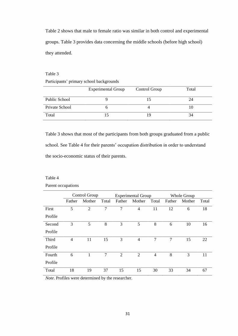
Table 2 shows that male to female ratio was similar in both control and experimental
groups. Table 3 provides data concerning the middle schools (before high school)
they attended.
Table 3
Participants’ primary school backgrounds
Experimental Group Control Group Total
Public School 9 15 24
Private School 6 4 10
Total 15 19 34
Table 3 shows that most of the participants from both groups graduated from a public
school. See Table 4 for their parents’ occupation distribution in order to understand
the socio-economic status of their parents.
Table 4
Parent occupations
Father Mother Total Father Mother Total Father Mother Total
First
Profile
5 2 7 7 4 11 12 6 18
Second
Profile
3 5 8 3 5 8 6 10 16
Third
Profile
4 11 15 3 4 7 7 15 22
Fourth
Profile
6 1 7 2 2 4 8 3 11
Total 18 19 37 15 15 30 33 34 67
Note. Profiles were determined by the researcher.
Control Group Experimental Group Whole Group

32
In Table 4, first profile consists of professions including doctors, engineers,
architects, lawyers, directors, and financial advisors. Second profile jobs were civil
servants, teachers, and nurses. Third profile includes parents who were retired or not
working. Fourth profile parents’ are accountants, self-employed, and painters. While
parents of students in the experimental group were mostly employed in first profile
jobs, parents from control group were mostly doing third profile jobs.
Data collection
Procedure
Two instruments, a limits and continuity readiness test (LCRT) and a mathematics
and technology attitudes scale (MTAS), were used during the pre-test period. After
the pre-test, limits and continuity concepts were taught with two different methods.
The researcher, also a teacher of the students, taught the concepts by using GeoGebra
to the experimental group. A fellow teacher taught the control group. Traditional
teaching methods were used to teach limits and continuity in the control group. After
the intervention, the post-tests were adminsitered. The post-test used two
instruments, a limits and continuity achievement test (LCAT) and MTAS. A written
permission was granted by MoNE to conduct the study at this school. See Appendix
6.
Instruments
Limits and continuity readiness test
This test originally consisted of 12 open-ended questions to test the readiness of
students for the limits and continuity topics. The first item is an adaptation of a
question that was asked in the university entrance exam in 1990 and this question
33
was removed from further analysis due to negative item-total correlation. The second
question was an adaptation of a question asked in the university entrance exam in
1997. The third question was adapted from a university entrance exam preparation
workbook. These three questions required a low-level of cognitive demand with
respect to the concepts of limits and continuity. The other nine questions were the
same as the ones used by Kepçeoğlu (2010) in their study. The pre-test questions
were evaluated to focus primarly on procedural knowledge. After the first question
was excluded from the study—a decision made based on reliability analysis—the
minimum score for the readiness test was 0 and the maximum score was 4 when total
score was divided by 11 in order to find the final pre-test readiness score (See
Appendix 1 for limits and continuity readiness test [LCRT] questions).
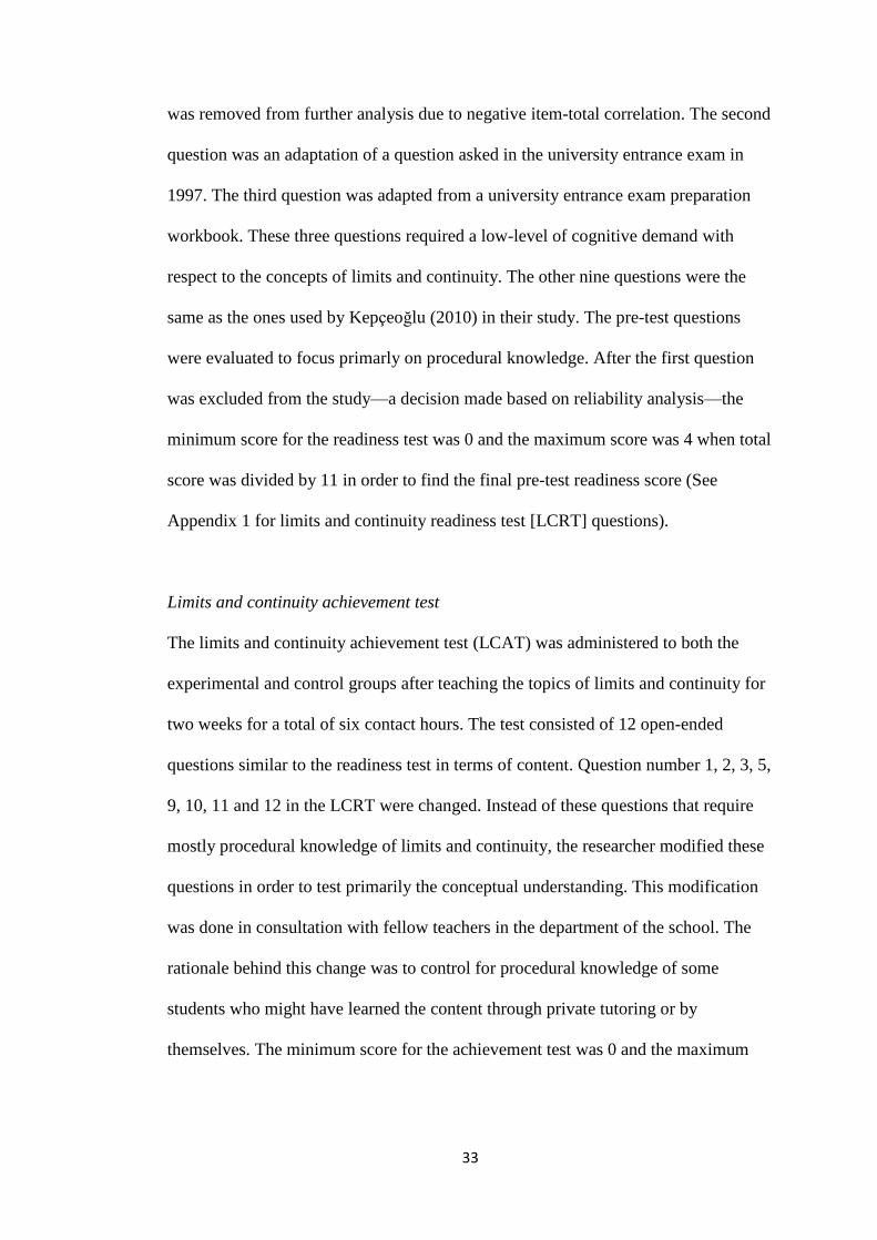
Limits and continuity achievement test
The limits and continuity achievement test (LCAT) was administered to both the
experimental and control groups after teaching the topics of limits and continuity for
two weeks for a total of six contact hours. The test consisted of 12 open-ended
questions similar to the readiness test in terms of content. Question number 1, 2, 3, 5,
9, 10, 11 and 12 in the LCRT were changed. Instead of these questions that require
mostly procedural knowledge of limits and continuity, the researcher modified these
questions in order to test primarily the conceptual understanding. This modification
was done in consultation with fellow teachers in the department of the school. The
rationale behind this change was to control for procedural knowledge of some
students who might have learned the content through private tutoring or by
themselves. The minimum score for the achievement test was 0 and the maximum

34
score was 4 when total score was divided by 12 in order to find the final post-test
achievement score (See Appendix 2 for LCAT questions).
Assessment criteria for LCRT and LCAT
The following assessment criteria were used in grading responses to the limits and
continuity readiness and achievement tests (cf. Kepçeoğlu, 2010). According to
Table 1, the possible minimum score was 0, and the possible maximum score was 4.
The answer key was prepared by the researcher and discussed with other teachers in
the school, including the teacher of the control group.
Table 5
Assessment criteria for LCRT and LCAT
Correct Partially
Correct
Wrong (1) Wrong (2) Unanswered
4 marks 3 marks 2 marks 1 mark 0 mark
Correct: The answer was totally correct.
Partially Correct: Some minor mistakes, including miscalculations.
Wrong(1): Error(s) were made at the very early stages of the steps required to
reach the solution or the process was not specified.
Wrong(2): There was a meaningful attempt but the answer was wrong.
Unanswered: No answer to the question or no meaningful attempt was
provided.
The mathematics and technology attitudes scale
The mathematics and technology attitudes scale (MTAS) developed by Pierce,
Stacey, and Barkatsas (2007) was used to examine the effects of the GeoGebra

35
software on student attitudes towards mathematics and technology. The researchers
evaluated this instrument to be leaner, shorter, and more understandable compared to
other scales. Furthermore, the survey avoided negative statements to prevent
complexity in meaning and to protect students from delving into negative thoughts in
the long term. The survey had five sub-scales.
(a) mathematical confidence (MC);
(b) confidence with technology (CT);
(c) attitude to learning mathematics with technology (MT);
(d) affective engagement (AE);
(e) behavioral engagement (BE).
For four of the sub-scales, MC, MT, MT and AE, a 5-point Likert-type with strongly
agree to strongly disagree responses was used. For the sub-scale BE, a similar
format—nearly always, usually, about half of the time, occasionally, hardly ever—
was used (See Appendix 3 for MTAS items). All the sub-scales have been scored
from 1 to 5 by computing the averages of responses within each factor.
Intervention
For the intervention, limits and continuity concepts were planned to be taught in
GeoGebra supported environment (dynamic graphs) to the experimental group. The
teacher was the researcher. Traditional teaching methods were used by a fellow
teacher in the control group class involved using projecting the content (still non-
dynamic graphs) to the board and in class discussions. Before the intervention
period, both teachers prepared the lesson plans and materials together. Each lesson

36
hour and activity was discussed in the department. Detailed explanation of each
lesson hour is given as follows:
First and second lesson hours
In the first lesson, both teachers explained the difference between value of the limit
of a function and a function converging to a particular value given that independent
variable is manipulated.
GeoGebra software including basic tools were introduced to students in the
experimental group in order for them to download and practice after school. This
introduction lasted for abut five minutes and students reported that the program was
user-friendly and they were able to use it with ease. In fact, students were observed
to be skilled in adapting to the GeoGebra environment. During the in-class
discussion, researcher created GeoGebra applets and worksheets for experimental
group, whereas the traditional group used paper-based worksheets that included non-
dynamic (still) graphs of the same functions. See Figure 1, Figure 2, and Figure 3 for
materials used in experimental group:

37
Figure 1. GeoGebra applet for limiting (first function)
Figure 2. GeoGebra applet for limiting (second function)

38
Figure 3. GeoGebra applet for limiting (third function)
First, the researcher explained to which value the function converges (left-hand and
right-hand) in the first figure. Students were expected to estimate to which value was
the function converging depending on the changing values of x. Some students used
the computer and showed the process with the pointer (mouse). This was the enactive
stage at which students attempted to show the left-hand and the right-hand limiting
process by using their pointers. The researcher asked students to inquire the value
where x = 2 while the function was jumping to y = 4. See Figure 1. Students
discussed that the function was converging to y = 2 when approached to x = 2 from
left or right, although the exact value of the function at that x value was y = 4. At the
end, researcher stated the limit notation and that if these two values were not equal,
limit would not exist.
Second, GeoGebra applet in Figure 2 was used to explain the limiting process for a
piece-wise function. The students observed and followed the teacher showing the
convergence on the graph. This observation stage in which the students were not

39
actively required to manipulate the function was considered as an activity for the
iconic stage. However, some students were engaged in Geogebra and showed the
convergence by themselves. The researcher encouraged all students to manipulate the
x values during their study time after school. Given the fact that the school was
boarding and all students were required to attend these study hours, it would be
expected that they used the program. Furthermore in the classroom, students were
asked to observe the limits of the function when x values approach -1, 0, 2, 3, 5 and 6
from left or right. They were asked to use the formal notation and determine whether
the limit existed or not. The students worked with the formal notation to connect
enactive, iconic and symbolic representations.
Third, concept of infinity was discussed with the students on a GeoGebra applet with
the help of the graphs in Figure 3. While x value was approaching to 3, they
discovered that the value of the function had been getting bigger and bigger, getting
closer to an idea, called the infinity. In addition, the students expressed their opinions
about the relationship between the symbolic equation of the function and the idea of
infinity. As the final activity of the first and second lesson hours, the researcher
requested the students to fill out a table, which is shown in Figure 4:
Figure 4. Table for algebraic calculations of the approaches

40
The students could use either a calculator or the GeoGebra program to calculate the
values during this activity. The researcher allowed the students to use laptops while
the researcher was providing feedback. At the end, the researcher draw the graphs of
functions by using GeoGebra. Students had the opportunity to compare the values
they have found and check their findings in the table.
In the meantime, the teacher in the control group used two hard-copy worksheets
which included the same examples of functions. See Appendix 7 for the paper-based
worksheets.
In the last ten minutes of the lessons, the limiting process was summarized in the
same manner to both groups, including a conversation about Niels Henrik Abel, a
prominent mathematician, whose contribution to limits and continuity concepts was
remarkable. In addition, the teachers requested the students to think about the
relationship between polygons and circles. This was given as homework to be
discussed during the next lesson.
Third and Fourth Lesson Hours
In the beginning of the third lesson, a GeoGebra applet was used (GeoGebra Tube,
2015), to show the relationship between polygons and circles in the homework. The
aim of this applet was to make students to understand that a polygon becomes to a
circle when the number of its sides goes to infinity. See Figure 5 for an interface of
that applet.

41
Figure 5. GeoGebra applet for investigating relations between circles and polygons
In that activity, n indicated the number of the sides of the polygon. The experimental
group students were demonstrated that the polygon approached to a circle when the
number of its sides increased. That could be considered the iconic stage. Students
also observed in a tabular representation that the ratio of the area of the polygon to
that of the circle would approach to 100%. The allocated time for this activity was
ten minutes.
Second, another GeoGebra applet was used to enable students to explore the limiting
process where the function was not undefined. Students initially investigated the
limits value and the exact value of the function individually, and students explained
their findings to their peers by using the GeoGebra applet. Figure 6 shows the
snapshot of the applet.

42
Figure 6. GeoGebra applet for limiting (six different functions)
The activity which is shown in Figure 6 was for the function g(x) = |x-|x-5||. The
students used two separate sliders to manipulate the x values from left or right of x =
3. The table at the far right side of the Figure 6 showed left-hand, right-hand and the
exact values of the function around x = 3. The students compared the values of the
table and their initial estimations. This was considered as an activity for both
enactive and iconic stages. The allocated time for this activity was 20 minutes.
In the third activity, the students discovered the basic limit properties for a variety of
functions types including polynomial functions, radical functions, and absolute value
functions. This was planned to be a group work activity. A GeoGebra applet, which
can be seen in Figure 7, was used for this activity. The allocated time for this activity
was 20 minutes. The students were also asked to fill out a table, which was shown in
Figure 8.
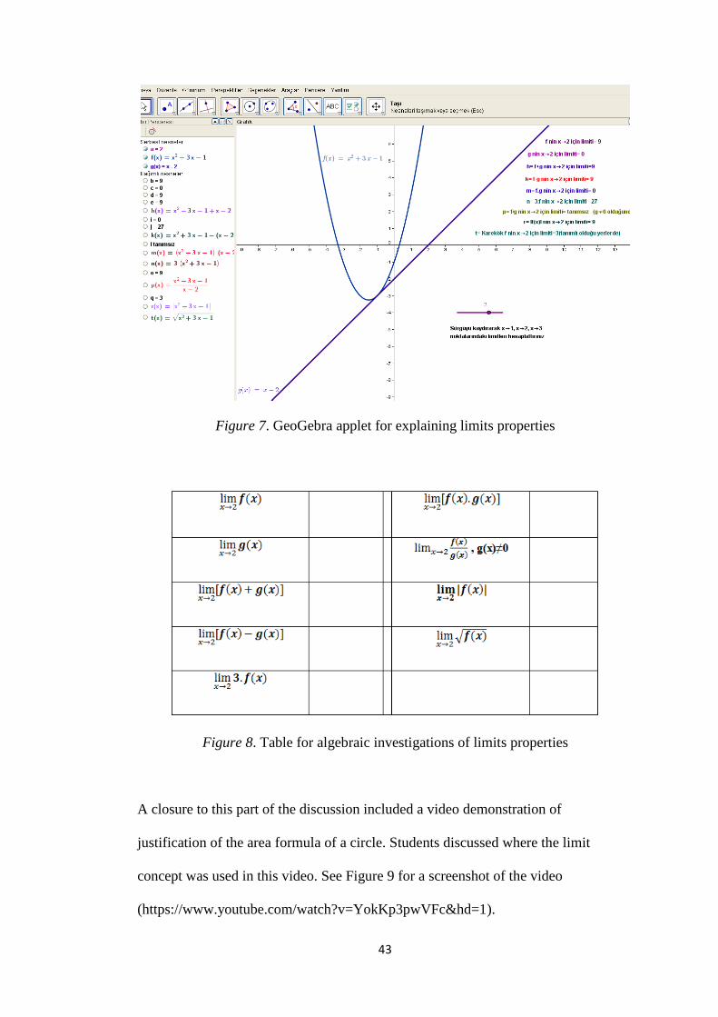
43
Figure 7. GeoGebra applet for explaining limits properties
Figure 8. Table for algebraic investigations of limits properties
A closure to this part of the discussion included a video demonstration of
justification of the area formula of a circle. Students discussed where the limit
concept was used in this video. See Figure 9 for a screenshot of the video
(https://www.youtube.com/watch?v=YokKp3pwVFc&hd=1).
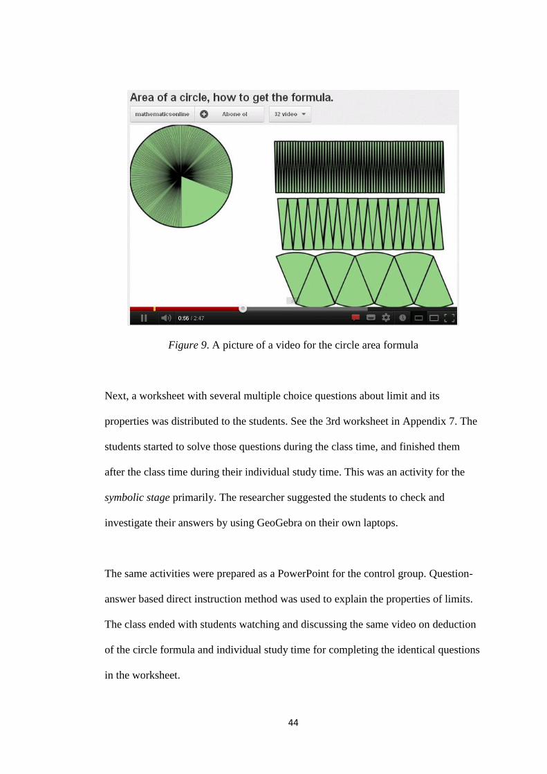
44
Figure 9. A picture of a video for the circle area formula
Next, a worksheet with several multiple choice questions about limit and its
properties was distributed to the students. See the 3rd worksheet in Appendix 7. The
students started to solve those questions during the class time, and finished them
after the class time during their individual study time. This was an activity for the
symbolic stage primarily. The researcher suggested the students to check and
investigate their answers by using GeoGebra on their own laptops.
The same activities were prepared as a PowerPoint for the control group. Question-
answer based direct instruction method was used to explain the properties of limits.
The class ended with students watching and discussing the same video on deduction
of the circle formula and individual study time for completing the identical questions
in the worksheet.

45
Fifth and sixth lesson hours
At the first activity of the last two periods of intervention, continuity concept was
explained, discussed, and explored on graphs prepared with GeoGebra. See Figure
10 for the first Geogebra applet for continuity.
Figure 10. GeoGebra applet for continuity
The students were supposed to discover when a function was continuous or
discontinuous by investigating the applet that included three different functions. At
the end of the activity, the students were expected to discover that a function was
continuous if and only if its left-hand limit and right-hand limit around an x value
and exact value of the function at that value were the same. The allocated time for
this enactive stage activity was ten minutes.
Second, several properties about limits of functions that approach to infinity were
discussed with the students. For example, the sum of two functions that both had
been going to infinity was also going to infinity. After that, the graph of the function
y=1/x was drawn with GeoGebra in order to understand its behaviour when x

46
approaches to 0+, 0
-, and . The allocated time for this enactive stage activity
was ten minutes. See Figure 11 for an image of that GeoGebra activity.
Figure 11. GeoGebra applet for investigation of the function y=1/x around zero
Third, some trigonometric functions were drawn with GeoGebra, and the students
were expected to express their findings about the limits of trigonometric functions
and their continuity. Figure 12 was an image of the graphs of two trigonometric
functions drawn with GeoGebra.

47
Figure 12. GeoGebra applet for trigonometric limits and continuity
In this activity, students were expected to understand that finding the value that
functions converge to (the limit) was identical to finding the value of the function if
the function was not undefined at that value of x. The students discussed whether
there was an x value that made the function discontinous by comparing the
functions’ equations and graphs. Ten minutes were allocated for the activity.
After the students gained some general insights into limits of trigonometric
functions with the help of the third worksheet (this was given as homework in
previous lesson), students were asked to think about the y=sinx/x when x approaches
to zero. In fact, some students claimed that they could resolve the 0/0 situation in
sinx/x function through factorization. When they could not do so, the GeoGebra
graphs were used to show that the limit was equal to 1. Figure 13 was an image of
that activity.

48
Figure 13. GeoGebra applet for investigation of the function y=sinx/x around zero
The students observed that the left-hand and right-hand limits of f(x)=sinx/x as x
approaches to zero was equal to 1 despite their observation that f(0) was 0/0. In order
to prove algebraically, the researcher gave the students an image as a clue which is
shown in Figure 14 as an iconic stage activity.
Figure 14. A picture given as a clue to prove the limit of sinx/x around zero.
The students tried to find out sinx x tanx as a group work by the help of that
clue. The students had some difficulties during that activity and teacher had to help

49
the groups. In the proof process, symbolic stage was the purpose of the activity. 20
minutes were given for students to prove this.
After the proof section of the lesson, the teacher explained several implications of
sinx/x property, including
,
or
.
Then, the researcher distributed a worksheet including eight questions as a further
symbolic stage activity. See worksheet 4 in the Appendix 7. The allocated time for
those eight questions was ten minutes, and the students used GeoGebra by entering
the equation of the functions if they needed to observe the behaviours of their graphs,
which might be considered the enactive and iconic stages.
The last part of the lesson was based on continuity. In order to understand the
discontinous points of given functions, the researcher used a GeoGebra applet, which
is shown in Figure 15.

50
Figure 15. GeoGebra applet for continuity (twelve different functions)
On this applet, the students worked out twelve different functions to discover limits
as x approaching some particular value, and continuous-discontinuous values and
intervals. Four of the functions are shown in Figure 15. The students discussed the
relations between the equations of the functions and x-values where the function was
discontinuous. Students changed the x values with the pointer (mouse) to manipulate
independently. At the end, there was a class discussion about the infinity and x
values, which makes the function indefinite or undefined on the graphs of functions.
The allocated time for this activity was about 25 minutes.
The researcher distributed a worksheet that included eight continuity questions. See
Appendix 7 (worksheet 5). Some students could finish solving these questions in the
class whereas others had work left during their individual study time after school.

51
For the fifth and sixth lessons, the control group students given the same questions,
the same activities with still pictures.
After the intervention period was finished, four lesson periods were assigned to the
groups to solve additional multiple choice and open-ended questions before the post-
test. The teachers allowed students to solve questions from their own workbooks, or
a worksheet that the teachers handed out. Some students from the experimental
group used GeoGebra program during those extra lessons to investigate some graphs
and limits. See Appendix 7 (worksheet 6) for the last set of worksheets given to both
groups.
The teaching strategy for the intervention (experimental group) was to use enactive
stage activities through the manipulation of variables on GeoGebra. That initial stage
was used to help students move on to iconic (non-dynamic) graphs and finally to the
symbolic representations of functions with respect to their limits and continunity.
Students who needed to refer back to the enactive stage activities were allowed to do
so in the class or during their individual study time. In the control group; however,
only the iconic stage was emphasized before the symbolic stage. Thus, the difference
was directly related to where students started their journey: enactive -> iconic ->
symbolic in the experimental group; in contrast to iconic -> symbolic in the control
group.

52
Reliability and validity
The score reliabilities for LCRT, LCAT, and MTAS were estimated by using
Cronbach’s alpha, one of the most common internal consistency analysis methods.
For MTAS, Cronbach’s alpha was calculated for each factor separately. High alpha
coefficients (above .7) are generally considered to indicate high internal consistency
of the scores (Bryman & Cramer, 2005).
Table 6
Item total statistics of LCRT and LCAT scales
LCRT Scale LCAT Scale
Question
Number
Corrected Item-
Total Correlation
Cronbach’s alpha
if Item deleted
Corrected Item-
Total Correlation
Cronbach’s alpha
if Item deleted
LCT1 -.21 .58 .52 .85
LCT2 .15 .52 .34 .86
LCT3 .37 .47 .34 .86
LCT4 .19 .51 .45 .86
LCT5 .19 .51 .52 .85
LCT6 .16 .52 .67 .84
LCT7 .15 .52 .64 .84
LCT8 .40 .48 .71 .84
LCT9 .30 .48 .56 .85
LCT10 .31 .48 .53 .85
LCT11 .27 .49 .73 .84
LCT12 .28 .49 .61 .85
In LCRT scale, the first question was needed to be removed because it had a negative
corrected item-total correlation, meaning that the item was not measuring a construct
similar to that of the rest of the questions (Pallant, 2001). Thus, the final version
LCRT included 11 questions while the final version of LCAT was kept as a 12
question test.

53
Table 7
Item total statistics of MTAS pre-test and MTAS post-test scales
Note: *Items under this factor are not included in the final version.
MTAS Pre-Test MTAS Post-Test
MTAS Items
Corrected Item-
Total
Correlation
Cronbach’s
alpha if Item
deleted
Corrected Item-
Total
Correlation
Cronbach’s
alpha if Item
deleted
Behavioral Engagement (BE)*
I concentrate hard in
mathematics .06 .32 .11 .63
I try to answer questions
the teacher asks -.03 .35 .55 .12
If I make mistakes, I work
until I have corrected
them
.50 -.20 .35 .35
If I can’t do a problem, I
keep trying different ideas .08 .24 .20 .46
Technology Confidence (TC)
I am good at using
computers .82 .84 .85 .90
I am good at using things
like VCRs, DVDs, MP3s
and mobile phones
.75 .90 .75 .94
I can fix a lot of computer
problems .82 .84 .29 .88
I am quick to learn new
computer software needed
for school
.80 .86 .85 .90
Mathematics Confidence (MC)
I have a mathematical
mind .77 .86 .86 .95
I can get good results in
mathematics .69 .89 .89 .94
I know I can handle
difficulties in
mathematics
.82 .85 .91 .93
I am confident with
mathematics .82 .84 .92 .93
Affective Engagement (AE)
I am interested to learn
new things in
mathematics
.77 .67 .74 .72
In mathematics you get
rewards for your effort .46 .84 .54 .84
Learning mathematics is
enjoyable .70 .71 .80 .69
I get a sense of
satisfaction when I solve
mathematics problems
.59 .77 .58 .82
Learning Mathematics with Technology (MT)
I like using DGS for
learning mathematics .47 .58 .65 .82
Using DGS is worth the
extra effort .09 .84 .57 .86
Mathematics is more
interesting when using
DGS
.70 .45 .81 .75
DGS help me learn
mathematics better .70 .44 .73 .79

54
According to the analysis of Cronbach’s alpha for MTAS pre-test, the BE items
needed to be removed in view of corrected item total correlation values which were
low. In addition, the second item of MT scale was also removed due to low item-total
correlation.
Table 8
Final Cronbach’s alpha values
Cronbach’s alpha N of items
Pre Test Post Test Pre Test Post Test
LCRT (Pre Test)
LCAT (Post Test) .59 .86 11 12
TC .89 .93 4 4
MC .89 .95 4 4
AE .80 .82 4 4
MT .84 .86 3 3
Note: MC: Mathematics Confidence; TC: Technology Confidence; AE: Affective
Engagement; MT: Learning Mathematics with Technology
Thus, as evidence of validity, the researcher used the following methods:
(a) a pilot study;
(b) expert views of a mathematics education professor;
(c) views of a mathematics teacher from outside the school where the study
was conducted;
(d) views of mathematics teachers from within the school; and
(e) an external rating to assess the LCRT and LCAT.
Data analysis
First, data were explored in terms of normality and outliers by using the statistics
software SPSS version 15. Any divergence from normality was examined in terms of
55
the standardized scores, skewness, kurtosis, and P-P plots (Tabachnick & Fidell,
2007). No outliers or missing scores were detected.
Second, descriptive statistics for each item were analyzed to have a better
understanding of how the participants responded to each item on the average. In
addition, non-parametric two-sample Mann-Whitney U test was aused to understand
the mean rank differences between control and experimental groups at the item level.
Effect sizes were estimated with the formula
This r effect size was later converted to Cohen’s d for an easier understanding of the
size of the effect (DeCoster, 2009).
Third, to answer the research questions:
(a) paired sample t-tests were used to determine whether there were
statistically significant pre-test and post-test score differences on the average within
either control or experimental group internally;
(b) independent samples t-tests were used to determine whether there was a
difference between the control and experimental group gain scores. Gain scores were
computed by subtracting the pre-test score average from the post-test average as the
number of items were not equal in LCRT and LCAT;
(c) Hence, effect sizes which helped researcher understand the sizes of the
impact between control and experimental groups at factor level were estimated with
Cohen’s d.

56
Four, bivariate correlations for determining whether there was a statistically
significant relationship between the students’ learning and attitudes were applied at
the factor level. Bivariate correlations were estimated between each pair of factors
with Pearson’s product-moment correlation coefficient r. Low correlations between
MTAS, LCRT or LCAT scores provided the evidence to not conduct a multivariate
analysis.

57
CHAPTER 4: RESULTS
Conceptual understanding in limits and continuity
Impact at the question level
Data from LCRT and LCAT questions were analyzed in terms of percent
distributions of student responses. Table 9 and Table 10 present the percent
distribution for each the LCRT question.
Table 9
Percent distribution of responses to each LCRT question
Correct
(4)
Partially
Correct (3)
Wrong 1
(2)
Wrong 2
(1)
Unanswered
(0)
Question
Number
EG* CG** EG CG EG CG EG CG EG CG
LCRT2 86.7 57.9 6.7 0 0 10.5 6.7 21.1 0 10.5
LCRT3 33.3 5.3 0 0 33.3 42.1 26.7 52.6 6.7 0
LCRT4 0 5.3 6.7 5.3 0 5.3 80.0 47.4 13.3 36.8
LCRT5 20.0 5.3 0 5.3 0 5.3 20.0 36.8 60.0 47.4
LCRT6 0 0 0 0 86.7 78.9 13.3 15.8 0 5.3
LCRT7 0 5.3 6.7 0 40.0 31.6 40.0 52.6 13.3 10.5
LCRT8 0 5.3 0 0 46.7 42.1 40.0 47.4 13.3 5.3
LCRT9 20.0 42.1 0 0 0 0 46.7 31.6 33.3 26.3
LCRT10 26.7 57.9 0 0 0 0 46.7 21.1 26.7 21.1
LCRT11 0 10.5 40.0 47.4 26.7 26.3 20.0 5.3 13.3 10.5
LCRT12 0 10.5 46.7 26.3 26.7 21.1 13.3 31.6 13.3 10.5
Note: *EG stands for the experimental group. **CG stands for the control group.
Table 9 shows that there were six LCRT questions (4, 6, 7, 8, 11, and 12th questions)
which none of the students from the experimental group could answer correctly;
whereas there was only one LCRT question (6th question) which none of the control

58
group students could answer correctly. Additionally, questions 6, 7, and 8 appeared
to have been the most difficult questions because they had a low percentage of
correctness for students in both of the groups. One other notable point was that 60%
of the students from the experimental group did not answer question 5.
Table 10
Percent distribution of responses to each LCAT question
Correct
(4)
Partially
Correct (3)
Wrong1
(2)
Wrong2
(1)
Unanswered
(0)
Question
Number
EG* CG** EG CG EG CG EG CG EG CG
LCAT1 6.7 0 13.3 0 66.7 26.3 6.7 73.7 6.7 0
LCAT2 66.7 47.4 0 5.3 33.3 26.3 0 21.1 0 0
LCAT3 13.3 5.3 0 5.3 33.3 21.1 40.0 63.2 13.3 5.3
LCAT4 73.3 36.8 6.7 21.1 0 15.8 6.7 26.3 13.3 0
LCAT5 53.3 21.1 6.7 0 33.3 36.8 0 26.3 6.7 15.8
LCAT6 73.3 21.1 6.7 15.8 0 10.5 13.3 52.6 6.7 0
LCAT7 80.0 5.3 6.7 15.8 13.3 26.3 0 52.6 0 0
LCAT8 66.7 10.5 0 15.8 6.7 36.8 26.7 31.6 0 5.3
LCAT9 73.3 10.5 13.3 26.3 0 26.3 6.7 21.1 6.7 15.8
LCAT10 93.3 47.4 0 26.3 6.7 21.1 0 0 0 5.3
LCAT11 26.7 10.5 60.0 36.8 13.3 42.1 0 10.5 0 0
LCAT12 33.3 15.8 46.7 26.3 0 0 13.3 47.4 6.7 10.5
Note: *EG stands for experimental group. **CG stands for control group.
Table 10 shows that the percentage of totally correct answers of the experimental
group was higher than that of the control group for all LCAT questions. One
remarkable point is that 80% of experimental group students answered the 7th
question totally correct, as compared to only 5.3% of the control group students.
Similar situation existed for questions number 8 and 9. The first question of the
LCAT seems to have been the most difficult, in view of its low correctness
percentage for both of the groups.

59
Question level location statistics were calculated in order to have a better
understanding of how the students responded to the questions as a whole. See Table
11 and Table 12 for the item level location statistics.
Table 11
Question level location statistics for each LCRT item
The location of the data showed a variance for the LCRT in terms of the accuracy of
the answers to the test questions. The first question and the last three questions of the
LCRT were centered around modes of 3 and 4 which means that most of the
questions were partially correct or totally correct. However, the rest of the questions
except 5 were centered around the modes of 1 or 2 which means that they were
mostly partially wrong or totally wrong. The fifth question was centered around a
mode of 0 which means that it was mostly unanswered.
Question Number Median Mode Range
LCRT2 4 4 4
LCRT3 2 1 4
LCRT4 1 1 4
LCRT5 0 0 4
LCRT6 2 2 2
LCRT7 1 1 4
LCRT8 1 1-2 4
LCRT9 1 1 4
LCRT10 1 4 4
LCRT11 2.5 3 4
LCRT12 2 3 4

60
Table 12
Question level location statistics for each LCAT item
The location of the data for the LCAT was centered around a mode of 4, indicating
that the most of the students in the sample answered the questions correctly.
Mann-Whitney U test statistics
First, a non-parametric two-sample Mann-Whitney U test was conducted at the
question level for each LCRT and LCAT item. Table 13 shows the statistical
significance of the difference between the mean ranks of two independent groups—
control group and the experimental group with regard to each question in the limits
and continuity readiness test. The Mann Whitney test allows comparison between the
mean ranks with critical U values. In addition, the p-calculated values column, which
indicates the probability, provides assistance in rejecting or failing to reject the null
hypothesis of no difference by considering its value to a pre-determined alpha value
of .05 (Huck, 2011).
Question Number Median Mode Range
LCAT1 2 1-2 4
LCAT2 4 4 3
LCAT3 1 1 4
LCAT4 4 4 4
LCAT5 2 2-4 4
LCAT6 3 4 4
LCAT7 2.5 4 3
LCAT8 2 4 4
LCAT9 3 4 4
LCAT10 4 4 4
LCAT11 3 3 3
LCAT12 3 3 4

61
Table 13
The Mann-Whitney U test statistics between experimental and control groups in each
LCRT item
Question Number Mann-Whitney U Z p-calculated
LCRT2 97.50 -1.94 > .05
LCRT3 102.50 -1.49 .14
LCRT4 122.50 -0.80 .42
LCRT5 133.50 -0.34 .73
LCRT6 130.50 -0.62 .53
LCRT7 133.00 -0.36 .72
LCRT8 132.00 -0.40 .69
LCRT9 113.50 -1.07 .28
LCRT10 104.00 -1.43 .15
LCRT11 106.50 -1.32 .19
LCRT12 131.50 -0.40 .70
The results of the non-parametric two-sample Mann Whitney U test showed that
there was no statistically significant difference in any of the LCRT items between
mean rank scores of the control and experimental groups (for all the questions p >
.05).
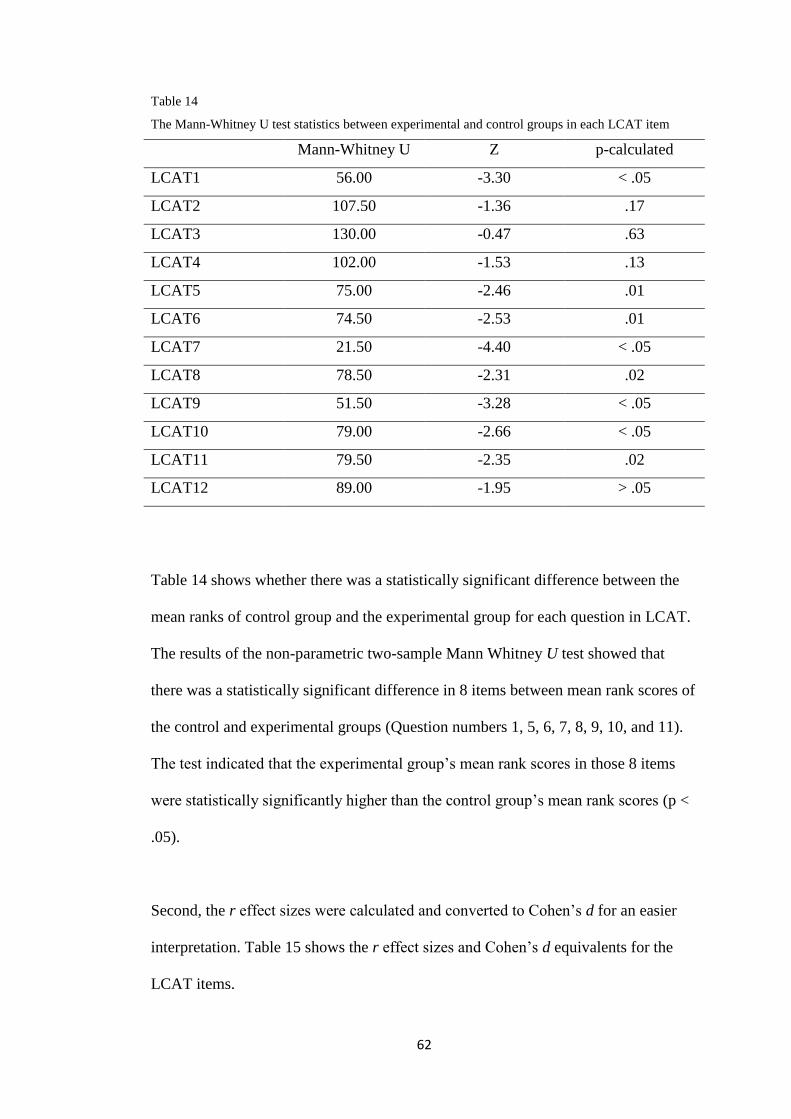
62
Table 14
The Mann-Whitney U test statistics between experimental and control groups in each LCAT item
Mann-Whitney U Z p-calculated
LCAT1 56.00 -3.30 < .05
LCAT2 107.50 -1.36 .17
LCAT3 130.00 -0.47 .63
LCAT4 102.00 -1.53 .13
LCAT5 75.00 -2.46 .01
LCAT6 74.50 -2.53 .01
LCAT7 21.50 -4.40 < .05
LCAT8 78.50 -2.31 .02
LCAT9 51.50 -3.28 < .05
LCAT10 79.00 -2.66 < .05
LCAT11 79.50 -2.35 .02
LCAT12 89.00 -1.95 > .05
Table 14 shows whether there was a statistically significant difference between the
mean ranks of control group and the experimental group for each question in LCAT.
The results of the non-parametric two-sample Mann Whitney U test showed that
there was a statistically significant difference in 8 items between mean rank scores of
the control and experimental groups (Question numbers 1, 5, 6, 7, 8, 9, 10, and 11).
The test indicated that the experimental group’s mean rank scores in those 8 items
were statistically significantly higher than the control group’s mean rank scores (p <
.05).
Second, the r effect sizes were calculated and converted to Cohen’s d for an easier
interpretation. Table 15 shows the r effect sizes and Cohen’s d equivalents for the
LCAT items.

63
Table 15
Effect sizes in each LCAT item
Items r Cohen’s d
LCAT1 .56 1.35
LCAT2 .23 0.47
LCAT3 .08 0.16
LCAT4 .26 0.54
LCAT5 .41 0.90
LCAT6 .43 0.95
LCAT7 .74 2.20
LCAT8 .39 0.84
LCAT9 .55 1.31
LCAT10 .45 1.00
LCAT11 .40 0.87
LCAT12 .33 0.70
Table 15 shows that some of the effect sizes could be considered to indicate a
practical difference when they were compared to the pilot study’s effect size or
average effect size in similar studies (See Table 31). Thus, there was a very large
difference between the groups in question 7, 1, and 9, in favour of the experimental
group.
Impact at the test level
In order to determine whether there was a statistically significant improvement in
both group of students’ conceptual understanding, a paired sample t-test was used.
See Table 16 for the groups’ mean, standard deviation, t-value, df-value, and p-
calculated values.
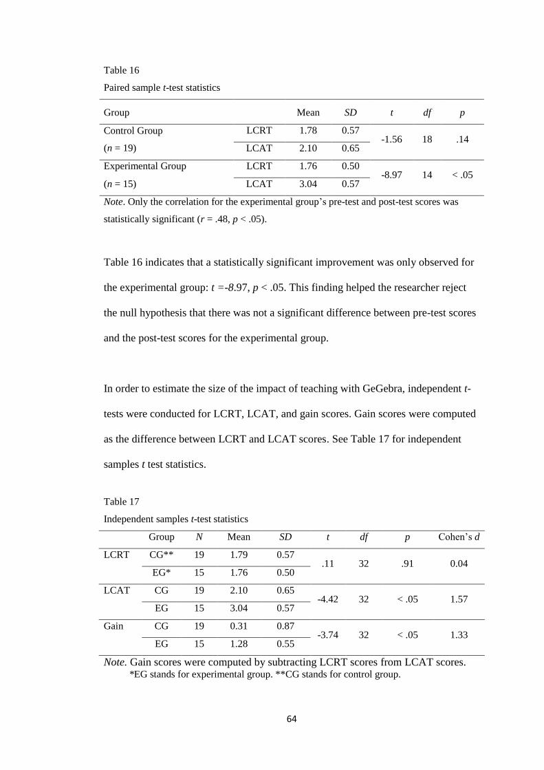
64
Table 16
Paired sample t-test statistics
Group Mean SD t df p
Control Group
(n = 19)
LCRT 1.78 0.57 -1.56 18 .14
LCAT 2.10 0.65
Experimental Group LCRT 1.76 0.50 -8.97 14 < .05
(n = 15) LCAT 3.04 0.57
Note. Only the correlation for the experimental group’s pre-test and post-test scores was
statistically significant (r = .48, p < .05).
Table 16 indicates that a statistically significant improvement was only observed for
the experimental group: t =-8.97, p < .05. This finding helped the researcher reject
the null hypothesis that there was not a significant difference between pre-test scores
and the post-test scores for the experimental group.
In order to estimate the size of the impact of teaching with GeGebra, independent t-
tests were conducted for LCRT, LCAT, and gain scores. Gain scores were computed
as the difference between LCRT and LCAT scores. See Table 17 for independent
samples t test statistics.
Table 17
Independent samples t-test statistics
Group N Mean SD t df p Cohen’s d
LCRT CG** 19 1.79 0.57 .11 32 .91 0.04
EG* 15 1.76 0.50
LCAT CG 19 2.10 0.65 -4.42 32 < .05 1.57
EG 15 3.04 0.57
Gain
CG 19 0.31 0.87 -3.74 32 < .05 1.33
EG 15 1.28 0.55
Note. Gain scores were computed by subtracting LCRT scores from LCAT scores. *EG stands for experimental group. **CG stands for control group.

65
What is the impact of learning limits and continuity concepts with GeoGebra on
G&T students’ conceptual understanding?
First, there was not a statistically significant difference between the control group
and experimental group with respect to their LCRT scores on the average: t = 0.11, p
> .05. According to this finding, the researcher did not reject the null hypothesis that
there was not a statistically significant difference between the control and
experimental groups in LCRT. Thus, students in both groups were assumed to have a
similar level of knowledge on limits and continuity before the intervention.
Second, there was a statistically significant difference between the control group and
experimental group with respect to the LCAT scores on the average: t = -4.42, p <
.05, Cohen’s d = 1.57. According to this finding, the researcher rejected the null
hypothesis that there was not a significant difference between the groups in LCAT.
Thus, it was found that the students in the experimental group had a more advanced
conceptual understanding of limits and continuity at the end of the intervention.
Finally, the results indicated that there was a statistically significant difference
between the control group’s gain scores and the experimental group’s gain scores on
the average: t = -3.74, p < .05, Cohen’s d = 1.33. According to this finding,
researcher rejected the null hypothesis that there was not a significant difference
between the groups in gain scores. Thus, it was found that the students in the
experimental group had developed a more advanced conceptual understanding of
limits and continuity after the intervention.

66
The effect sizes for the comparison of the groups on the LCRT, the LCAT and gain
limits scores were considered to indicate a practical difference when compared to the
effect size estimated in the pilot study and average effect size in similar studies (See
Table 31).
Attitudes towards technology in mathematics education
Impact at the item level
PreMTAS and PostMTAS items were analyzed in terms of percent distributions of
students’ responses.
Table 18
Percent distribution of responses to each MTAS pre-test item
Strongly
disagree
Disagree Not sure Agree Strongly
agree
EG* CG** EG CG EG CG EG CG EG CG
PreTC1 13.3 5.3 6.7 10.5 20.0 31.6 40.0 26.3 20.0 26.3
PreTC2 0 0 6.7 0 6.7 21.1 53.3 52.6 33.3 26.3
PreTC3 20.0 15.8 33.3 26.3 20.0 26.3 20.0 5.3 6.7 26.3
PreTC4 13.3 21.1 13.3 15.8 33.3 15.8 13.3 15.8 26.7 31.6
PreMC1 0 10.5 0 15.8 13.3 21.1 46.7 42.1 40.0 10.5
PreMC2 0 5.3 0 5.3 0 31.6 53.3 47.4 46.7 10.5
PreMC3 0 0 0 10.5 20.0 21.1 46.7 57.9 33.3 10.5
PreMC4 6.7 5.3 0 5.3 20.0 36.8 40.0 42.1 33.3 10.5
PreAE1 0 0 13.3 15.8 6.7 26.3 33.3 47.4 46.7 10.5
PreAE2 0 10.5 6.7 15.8 33.3 26.3 46.7 26.3 13.3 21.1
PreAE3 0 0 6.7 15.8 13.3 26.3 33.3 42.1 46.7 15.8
PreAE4 0 0 0 5.3 13.3 5.3 26.7 36.8 60.0 52.6
PreMT1 33.3 15.8 13.3 42.1 33.3 31.6 13.3 10.5 6.7 0
PreMT3 20.0 10.5 26.7 42.1 40.0 42.1 6.7 5.3 6.7 0
PreMT4 13.3 21.1 33.3 42.1 33.3 26.3 20.0 10.5 0 0
Note: *EG stands for experimental group. **CG stands for control group. PreTC:
Technology confident pre test questions. PreMC: Mathematics confident pre test questions.
PreAE: Affective engagement pre test questions. PreMT: Learning mathematics with
technology pre test questions.

67
Table 18 shows that students from the experimental group did not strongly disagree
with most of the items in the MTAS pre-test. However, in the preMT, none of the
items were answered with strongly agree by either group. Table 19 indicates that the
students from the experimental group were not generally in strong disagreement with
the items in the MTAS post-test. On the other hand, none of the students from the
control group strongly agreed with any of the items of the postMT.
Table 19
Percent distribution of responses to each MTAS post-test item
Strongly
disagree
Disagree Not sure Agree Strongly
agree
EG* CG** EG CG EG CG EG CG EG CG
PostTC1 0 5.3 40.0 15.8 13.3 26.3 33.3 26.3 13.3 26.3
PostTC2 0 0 13.3 10.5 26.7 26.3 46.7 31.6 13.3 31.6
PostTC3 33.3 10.5 6.7 36.8 33.3 15.8 20.0 10.5 6.7 26.3
PostTC4 13.3 10.5 20.0 21.1 26.7 26.3 26.7 21.1 13.3 21.1
PostMC1 0 10.5 0 15.8 26.7 15.8 40.0 42.1 33.3 15.8
PostMC2 0 5.3 0 5.3 6.7 26.3 53.3 52.6 40.0 10.5
PostMC3 0 5.3 0 10.5 20.0 26.3 33.3 42.1 46.7 15.8
PostMC4 6.7 10.5 0 15.8 20.0 15.8 33.3 42.1 40.0 15.8
PostAE1 0 5.3 6.7 15.8 6.7 26.3 46.7 42.1 40.0 10.5
PostAE2 0 10.5 13.3 10.5 20.0 31.6 40.0 15.8 26.7 31.6
PostAE3 0 5.3 0 10.5 13.3 36.8 40.0 31.6 46.7 15.8
PostAE4 0 0 0 0 6.7 10.5 40.0 42.1 53.3 47.4
PostMT1 0 36.8 33.3 31.6 20.0 26.3 40.0 5.3 6.7 0
PostMT3 0 36.8 26.7 26.3 20.0 26.3 33.3 10.5 20.0 0
PostMT4 6.7 31.6 20.0 10.5 26.7 42.1 40.0 15.8 6.7 0
Note: *EG stands for experimental group. **CG stands for control group. PostTC:
Technology confident post test questions. PostMC: Mathematics confident post test
questions. PostAE: Affective engagement post test questions. PostMT: Learning
mathematics with technology post test questions.

68
Although Table 19 shows some similarities to Table 18, there were some slight
differences. One of the most remarkable differences was in the MT items. In the
MTAS pretest, some students from experimental group responded strongly disagree
for the preMT items. However, in the MTAS post test, none of the students from the
experimental group strongly disagreed for the items preMT1 and preMT3.
Item level location statistics were calculated in order to have a better understanding
of how the students responded to the MTAS items. See Table 20 and Table 21 for the
item level location statistics.
Table 20
Item level location statistics for each MTAS pre-test item
Median Mode Range
PreTC1 4 4 4
PreTC2 4 4 3
PreTC3 3 2 4
PreTC4 3 5 4
PreMC1 4 4 4
PreMC2 4 4 4
PreMC3 4 4 3
PreMC4 4 4 4
PreAE1 4 4 3
PreAE2 4 4 4
PreAE3 4 4 3
PreAE4 5 5 3
PreMT1 2 3 4
PreMT3 2.5 3 4
PreMT4 2 2 3
Note: PreTC: Technology confident pre test questions. PreMC: Mathematics confident pre
test questions. PreAE: Affective engagement pre test questions. PreMT: Learning
mathematics with technology pre test questions.

69
Table 21
Item level location statistics for each MTAS post-test item
The location of data was centered around a mode of 4 which stands for agree for both
MTAS pre-test and post-test items. However, the range values, which could help to
understand measures of data dispersion, were quite large.
Mann-Whitney U test statistics
A non-parametric two-sample Mann-Whitney U test was conducted at the item level
for each item in MTAS pre-test and post-test. Table 22 presents whether there was a
statistically significant difference between the mean ranks of two independent
Median Mode Range
PostTC1 3.5 4 4
PostTC2 4 4 3
PostTC3 3 2-3 3
PostTC4 3 3 4
PostMC1 4 4 4
PostMC2 4 4 4
PostMC3 4 4 4
PostMC4 4 4 4
PostAE1 4 4 4
PostAE2 4 5 4
PostAE3 4 4 4
PostAE4 4.5 5 2
PostMT1 2 2 4
PostMT3 3 2 4
PostMT4 3 3 4
Note: PostTC: Technology confident post test questions. PostMC: Mathematics confident
post test questions. PostAE: Affective engagement post test questions. PostMT: Learning
mathematics with technology post test questions.

70
groups—the control group and the experimental group—in attitudes towards use of
technology in mathematics education.
Table 22
The Mann-Whitney U test statistics between experimental and control groups in each MTAS
pre-test item
Mann-Whitney U Z p-calculated
PreTC1 139.50 -0.11 .91
PreTC2 128.50 -0.53 .60
PreTC3 120.50 -0.78 .43
PreTC4 140.50 -0.07 .94
PreMC1 72.00 -2.58 .01
PreMC2 59.00 -3.14 <.05
PreMC3 102.50 -1.52 .13
PreMC4 100.00 -1.56 .12
PreAE1 88.00 -1.99 > .05
PreAE2 122.50 -0.72 .47
PreAE3 90.00 -1.91 > .05
PreAE4 134.00 -0.33 .74
PreMT1 138.50 -0.14 .88
PreMT3 136.50 -0.22 .82
PreMT4 114.50 -1.01 .31
Note: PreTC: Technology confident pre test questions. PreMC: Mathematics confident pre
test questions. PreAE: Affective engagement pre test questions. PreMT: Learning
mathematics with technology pre test questions.
The results of non-parametric Mann-Whitney U test show that there was a
statistically significant difference in two items between the experimental group’s
mean rank scores and the control group’s mean rank scores (preMC1 and preMC2).
The results indicated that the experimental group’s mean rank scores were
statistically significantly higher than the control group’s mean rank scores for those
items. Both items belong to the domain MC: have a mathematical mind (MC1: z = -

71
2.58, p < .05, r = .44 and Cohen’s d = 0.99) and get good results in mathematics
(MC2: z = -3.14, r = .54 and Cohen’s d = 1.28).
Table 23
The Mann-Whitney U test statistics between experimental and control groups in each MTAS
post-test item
Mann-Whitney U Z p-calculated
PostTC1 118.50 -0.86 .39
PostTC2 122.00 -0.74 .46
PostTC3 118.50 -0.85 .39
PostTC4 134.00 -0.30 .76
PostMC1 99.50 -1.56 .12
PostMC2 76.50 -2.50 .01
PostMC3 86.00 -2.06 .04
PostMC4 99.50 -1.55 .12
PostAE1 77.00 -2.40 .16
PostAE2 125.00 -0.63 .53
PostAE3 71.50 -2.58 .01
PostAE4 132.00 -0.40 .68
PostMT1 58.50 -3.01 <.05
PostMT3 56.50 -3.06 <.05
PostMT4 89.00 -1.92 >.05
Note: PostTC: Technology confident post test questions. PostMC: Mathematics confident
post test questions. PostAE: Affective engagement post test questions. PostMT: Learning
mathematics with technology post test questions.
There was a statistically significant difference between the mean rank scores of the
experimental and control groups in five items: postMC2, postMC3, postAE3,
postMT1 and postMT3. The results show that the experimental group mean rank
scores were statistically significantly higher than the control group mean rank scores
for those items. Table 24 shows the effect sizes for all MTAS post-test items.
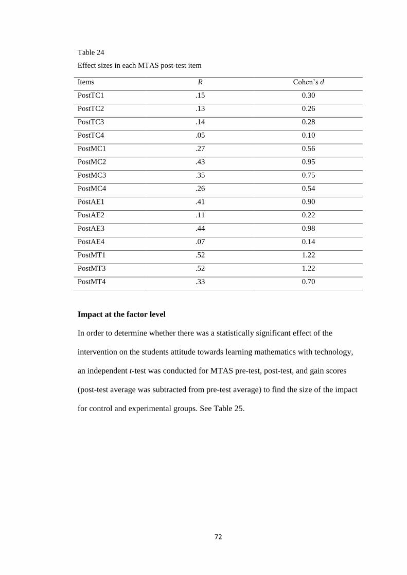
72
Table 24
Effect sizes in each MTAS post-test item
Impact at the factor level
In order to determine whether there was a statistically significant effect of the
intervention on the students attitude towards learning mathematics with technology,
an independent t-test was conducted for MTAS pre-test, post-test, and gain scores
(post-test average was subtracted from pre-test average) to find the size of the impact
for control and experimental groups. See Table 25.
Items R Cohen’s d
PostTC1 .15 0.30
PostTC2 .13 0.26
PostTC3 .14 0.28
PostTC4 .05 0.10
PostMC1 .27 0.56
PostMC2 .43 0.95
PostMC3 .35 0.75
PostMC4 .26 0.54
PostAE1 .41 0.90
PostAE2 .11 0.22
PostAE3 .44 0.98
PostAE4 .07 0.14
PostMT1 .52 1.22
PostMT3 .52 1.22
PostMT4 .33 0.70

73
Table 25
Independent t-test statistics for MTAS
Groups N Mean SD t df p
PreTC Control 19 3.46 1.14 0.25 32 .80
Experimental 15 3.37 1.02
PreMC Control 19 3.49 0.86 -2.64 32 .01
Experimental 15 4.20 0.66
PreAE Control 19 3.70 0.74 -1.60 32 .12
Experimental 15 4.12 0.78
PreMT Control 19 2.35 0.76 -0.61 32 .55
Experimental 15 2.53 1.00
PostTC Control 19 3.41 1.15 0.76 32 .45
Experimental 15 3.12 1.07
PostMC Control 19 3.46 1.08 -2.14 32 .04
Experimental 15 4.17 0.77
PostAE Control 19 3.66 0.81 -2.02 32 >.05
Experimental 15 4.20 0.73
PostMT Control 19 2.18 0.90 -3.59 32 <.05
Experimental 15 3.29 0.90
TCgain Control 19 -0.05 0.50 1.25 32 .22
Experimental 15 -0.25 0.39
MCgain Control 19 -0.02 0.66 0.04 28.00 .97
Experimental 15 -0.03 0.34
AEgain Control 19 -0.04 0.52 -0.67 32 .51
Experimental 15 0.08 0.54
MTgain Control 19 -0.18 0.86 -2.96 32 <.05
Experimental 15 0.76 0.98
Note. SD = standard deviation. p = pcalculated.
TC: Technology Confidence. MC: Mathematics Confidence. AE: Affective Engagement.
MT: Learning Mathematics with Technology.
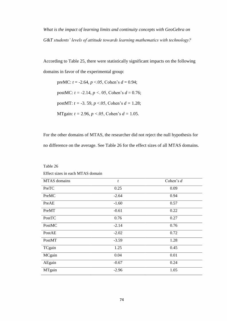
74
What is the impact of learning limits and continuity concepts with GeoGebra on
G&T students’ levels of attitude towards learning mathematics with technology?
According to Table 25, there were statistically significant impacts on the following
domains in favor of the experimental group:
preMC: t = -2.64, p <.05, Cohen’s d = 0.94;
postMC: t = -2.14, p <. 05, Cohen’s d = 0.76;
postMT: t = -3. 59, p <.05, Cohen’s d = 1.28;
MTgain: t = 2.96, p <.05, Cohen’s d = 1.05.
For the other domains of MTAS, the researcher did not reject the null hypothesis for
no difference on the average. See Table 26 for the effect sizes of all MTAS domains.
Table 26
Effect sizes in each MTAS domain
MTAS domains t Cohen’s d
PreTC 0.25 0.09
PreMC -2.64 0.94
PreAE -1.60 0.57
PreMT -0.61 0.22
PostTC 0.76 0.27
PostMC -2.14 0.76
PostAE -2.02 0.72
PostMT -3.59 1.28
TCgain 1.25 0.45
MCgain 0.04 0.01
AEgain -0.67 0.24
MTgain -2.96 1.05

75
Bivariate correlations between variables
Bivariate correlations were calculated between the continuous variables. See Table
27 and Table 28 for bivariate correlations between LCRT, LCAT and MTAS factors
according to the control and experimental groups separately:
Table 27
Bivariate correlations for control group (actual scores)
LCRT LCAT PreTC PreMC PreAE PreMT PostTC PostMC PostAE PostMT
LCRT 1 -.01 .13 .08 .12 .57* .19 .01 .23 .31
LCAT 1 .11 .38 .06 -.18 -.01 .59* .38 .13
PreTC 1 .07 -.56* .20 .90* .03 -.37 -.22
PreMC 1 .40 .25 -.13 .79* .48* .16
PreAE 1 .16 -.56* .38 .78* .40
PreMT 1 .29 -.01 .03 .57*
PostTC 1 -.23 -.46* -.18
PostMC 1 .66* .07
PostAE 1 .33
PostMT 1
Note. *Correlation is statistically significant at the .05 level.
TC: Technology Confidence. MC: Mathematics Confidence. AE: Affective Engagement. MT:
Learning Mathematics with Technology.
Some pairs of correlations, shown with an asterisk, were statistically significant for
the control group at the p < .05 level. The strongest positive correlation was
observed between the preTC scores and postTC scores and was evaluated as being
very strong (r2
= .81), indicating that students’ technology confidence in the pretest
was strongly correlated with students’ technology confidence in the posttest for the
control group. One other remarkable point in Table 27 was that the preTC
(technology confidence) scores were moderately negatively correlated with the
preAE scores, as were the preAE scores with the postTC scores (r2
= .31) for the
control group. Moreover, for the control group, only the pairs LCRT and preMT;
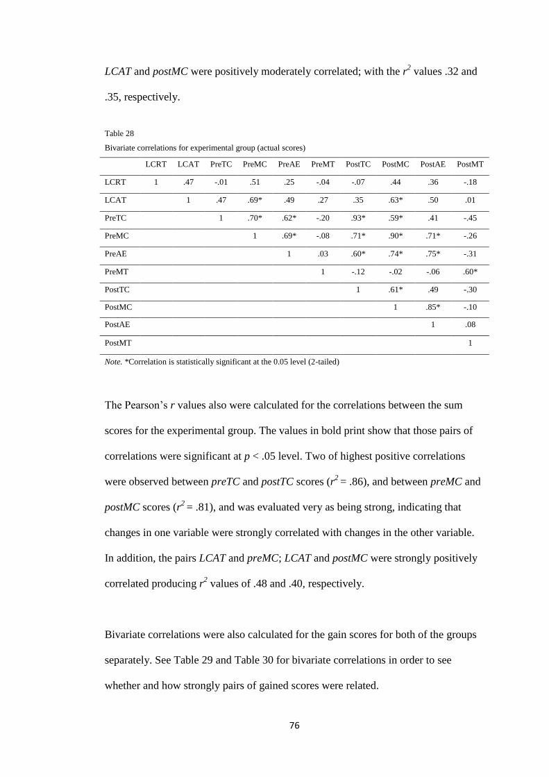
76
LCAT and postMC were positively moderately correlated; with the r2 values .32 and
.35, respectively.
Table 28
Bivariate correlations for experimental group (actual scores)
LCRT LCAT PreTC PreMC PreAE PreMT PostTC PostMC PostAE PostMT
LCRT 1 .47 -.01 .51 .25 -.04 -.07 .44 .36 -.18
LCAT 1 .47 .69* .49 .27 .35 .63* .50 .01
PreTC 1 .70* .62* -.20 .93* .59* .41 -.45
PreMC 1 .69* -.08 .71* .90* .71* -.26
PreAE 1 .03 .60* .74* .75* -.31
PreMT 1 -.12 -.02 -.06 .60*
PostTC 1 .61* .49 -.30
PostMC 1 .85* -.10
PostAE 1 .08
PostMT 1
Note. *Correlation is statistically significant at the 0.05 level (2-tailed)
The Pearson’s r values also were calculated for the correlations between the sum
scores for the experimental group. The values in bold print show that those pairs of
correlations were significant at p < .05 level. Two of highest positive correlations
were observed between preTC and postTC scores (r2
= .86), and between preMC and
postMC scores (r2
= .81), and was evaluated very as being strong, indicating that
changes in one variable were strongly correlated with changes in the other variable.
In addition, the pairs LCAT and preMC; LCAT and postMC were strongly positively
correlated producing r2 values of .48 and .40, respectively.
Bivariate correlations were also calculated for the gain scores for both of the groups
separately. See Table 29 and Table 30 for bivariate correlations in order to see
whether and how strongly pairs of gained scores were related.

77
Table 29
Bivariate correlations for control group (gain scores)
gainLimit gainTC gainMC gainAE gainMT
gainLimit 1 -.44 .43 .28 .34
gainTC 1 -.39 -.30 -.08
gainMC 1 .56* .20
gainAE 1 .11
gainMT 1
Note. *Correlation is statistically significant at the 0.05 level (2-tailed). GainLimit is the gain
scores between LCRT and LCAT.
Table 29 indicates that gainMC scores were moderately positively correlated with the
gainAE scores (r2
= .31), showing that changes in gainMC scores of students in the
control group were moderately correlated with the changes in gainAE scores.
Table 30
Bivariate correlations for experimental group (gain scores)
gainLimit gainTC gainMC gainAE gainMT
gainLimit 1 -.16 .08 -.12 -.16
gainTC 1 .10 .34 .20
gainMC 1 .26 .20
gainAE 1 .78*
gainMT 1
Note. *Correlation is statistically significant at the 0.05 level (2-tailed). GainLimit is the gain
scores between LCRT and LCAT.
In addition, Table 30 shows that gainAE scores were strongly positively correlated
with the gainMT scores (r2
= .61), indicating that changes in gainAE scores of
students in the experimental group were strongly correlated with the changes in
gainMT scores.

78
CHAPTER 5: DISCUSSION
Overview of the study
The main purpose of this study was to investigate the impact of teaching
mathematics with GeoGebra on 12th grade gifted and talented (G&T) students'
conceptual understanding of the limits and continuity concepts. The second purpose
was to investigate the impact of GeoGebra on students’ attitudes towards learning
mathematics with technology. This chapter starts with a summary of the major
findings and continues with a discussion of those findings. Discussion was written
with a meta-analytical approach in mind; thus, comparing the effect sizes deducted
from the current study to those deducted from other similar studies. The chapter ends
with concluding remarks, implications for practice, implications for further research,
and limitations of the study.
Major findings
Major findings of the study are stated below:
1) Students in the experimental group outperformed their peers in the control
group on the average in terms of gain scores in limits and continuity
conceptual understanding test. When the gain scores (post-test scores
subtracted from pre-test scores) were compared, there were 1.33 standard
deviations difference between two groups. This difference was statistically
significant (p < .05).

79
2) Students in the experimental group outperformed their peers in the control
group on the average in terms of gain scores in attitudes towards teaching
mathematics with technology (MT factor). There were 1.05 standard
deviations difference between two groups. This difference was statistically
significant (p < .05).
Some of the other findings were given as follows:
3) When post-test scores in limits and continuity test were compared, the
experimental group outperformed the control group with 1.57 standard
deviations. This difference was statistically significant (p < .05).
4) When the post-test scores and pre-test scores were compared within each
group, only the experimental group showed a statistically significant
improvement. The degree of conceptual understanding of limit and continuity
concepts was limited for the control group.
Table 31 summarizes some of the most relevant GeoGebra studies in the literature
and presents estimated effect sizes. These studies were selected based on similarity
of their methodology to that of the current study and use of GeoGebra as an example
of technology-supported mathematics education.
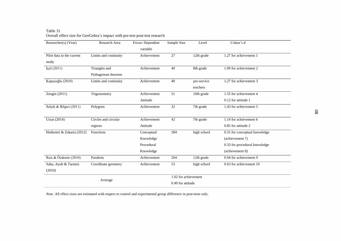
Table 31
Overall effect size for GeoGebra’s impact with pre-test post-test research
80
Researcher(s) (Year)
Research Area Focus: Dependent
variable
Sample Size Level Cohen’s d
Pilot data in the current
study
Limits and continuity Achievement 27 12th grade 1.27 for achievement 1
İçel (2011) Triangles and
Pythagorean theorem
Achievement
40 8th grade 1.09 for achievement 2
Kepçeoğlu (2010) Limits and continuity Achievement
40 pre-service
teachers
1.27 for achievement 3
Zengin (2011) Trigonometry Achievement
Attitude
51 10th grade 1.55 for achievement 4
0.12 for attitude 1
Selçik & Bilgici (2011) Polygons Achievement
32 7th grade 1.43 for achievement 5
Uzun (2014) Circles and circular
regions
Achievement
Attitude
42 7th grade 1.14 for achievement 6
0.85 for attitude 2
Hutkemri & Zakaria (2012) Functions Conceptual
Knowledge
Procedural
Knowledge
284 high school 0.55 for conceptual knowledge
(achievement 7)
0.33 for procedural knowledge
(achievement 8)
Reis & Özdemir (2010) Parabola Achievement 204 12th grade 0.94 for achievement 9
Saha, Ayub & Tarmizi
(2010)
Coordinate geometry Achievement 53 high school 0.63 for achievement 10
Average 1.02 for achievement
0.49 for attitude
Note. All effect sizes are estimated with respect to control and experimental group difference in post-tests only.

81
Discussion of the major findings
1) Students in the experimental group outperformed their peers in the control
group on the average in terms of gain scores in limits and continuity
conceptual understanding tests. When the gain scores (post test scores
subtracted from pre-test scores) were compared, there were 1.33 standard
deviations difference between two groups. This difference was statistically
significant (p < .05).
The best explanation to this finding is related to multiple representations theory. The
intervention that facilitates learning abstract mathematical constructs such as limits
and continuity, through multiple representations (enactive, iconic and symbolic
stages) can be a reason why students in the experimental group outperformed their
peers in the control group (Goldin, 2008). In fact, the evidence for dynamic geometry
software and GeoGebra in particular, providing teachers with tools to use these
stages simultaneously or one after the other is strong (Hohenwarter & Fuchs, 2004;
Zengin, Furkan, & Kutluca, 2012). When the intervention in this study is examined
more closely, it can be speculated that students benefit from the instruction that
successfully enables them to move on to the symbolic stage after extensive exposure
to activities that foster both the enactive and iconic stages. It can also be a possible
explanation that students can see multiple representations at the same time, such as
the one in lesson 1 and 2 (See Figure 2 and 3) where students can manipulate the
graph and see how the tabular representation changes.
The alternative; but related explanation to this finding is based on Kortenkamp’s
(1999) claim that dynamic geometry software can provide students with tools to

82
explore multiple perspectives in a single construction. For example, it is evident from
lesson 5 and 6 during the intervention that teachers can show at which points the
function is continous or not, while such software also allows for discussion on the
limiting process at a particular x value or at infinity (see Figure 15). Another
example can be given from the lesson 3 and 4 of the intervention of this study that
students can connect the limits to area calculations (See Figure 5). One last example
is related to an activity in lesson 1 and 2 where students can see the relationship
between the value that makes the function undefined and the value that an asymptote
appears (See Figure 3).
A final explanation is related to the characteristics of the population of the present
study. Thus, the difference between the experimental and control groups may have
originated from the fact that the participants of the study were gifted and talented
(G&T) students whose potentials can be realized if appropriate opportunities are
provided (Leikin, 2014), including the one provided by GeoGebra. Also, there is
evidence in the literature that G&T students adapt to environments in which students
have little prior experience, given the fact that students in the sample of this study
did not have any previous experience with GeoGebra (Leikin, 2014). A related
perspective is based on Renzulli’s (1986) three-ring model, which indicates that
G&T students’ ability, task commitment, and creativity flourish when they are
motivate. In fact, students in the study were encouraged to practice with GeoGebra
after school hours in a structured way.
Overall, this impact has been evaluated as noteworthy when the effect size was
compared to those estimated in İçel (2011), Kepçeoğlu (2010), Uzun (2014),

83
Hutkemri & Zakaria (2012), Reis & Özdemir (2010), and Saha, Ayub, & Tarmizi
(2010). The difference in size of the effect can be speculated to be based on the
possibility that some students express negative reactions to learning mathematics
with GeoGebra. It may be possible that participating students in other studies might
have evaluated GeoGebra as time-consuming or just confusing (Mehanovic, 2011).
2) Students in the experimental group outperformed their peers in the control
group on the average in terms of gain scores in attitudes towards teaching
mathematics with technology (MT factor). There were 1.05 standard
deviations difference between two groups. This difference was statistically
significant (p < .05).
.
The possible reasons behind the positive impact of GeoGebra on student attitudes
toward learning mathematics with technology are: (a) GeoGebra facilitates learning
and students become aware of it; (b) GeoGebra enhances visuality and renders the
topics tangible; and (c) GeoGebra is more appealing to students' learning styles due
to its multiple representations features (Aktümen, Yıldız, Horzum, & Ceylan, 2010;
Hohenwarter & Fuchs, 2004; Hohenwarter & Jones, 2007; Hohenwarter & Lavicza,
2009).
This finding can be considered important when compared to Zengin (2011) who did
not report any practical positive gain in terms of attitudes toward mathematics
(Cohen’s d = 0.12). However, it should be noted that the scope of the Zengin study
did not include measuring attitudes toward learning mathematics with technology.
Similarly in a study to investigate student attitudes toward geometry, Uzun (2014)

84
found some practical effect of GeoGebra (Cohen’s d = 0.85). However, neither of
these two studies could reach the impact achieved in the current study. This finding
can be explained with the different scopes of the studies. The current study focused
on measuring attitudes toward learning mathematics with technology rather than
attitude toward mathematics as a subject.
Implications for practice
In light of the findings, the following recommendations are made:
Subject-specific technology use should be encouraged at all schools across
the country. Thus, technologies that foster conceptual understanding in
mathematics such as GeoGebra should be the focus of Fatih project
technologies and limited resources should be allocated to similar effective
and freeware software.
Gifted and talented students are versatile learners. Hence, the program
developers and teachers of mathematics should consider that effective
programs, curricula, or teaching methods can help G&T students fulfil their
true potential. GeoGebra technology appears to offer an effective medium for
G&T students in learning mathematics and learning mathematics with a
applied focus. Thus, it is recommended that teachers of G&T students learn
to use GeoGebra technology effectively and to use similar DGS technology
with a student-centred approach.
At the secondary school level, teaching to the test or a classroom teaching
based on preparing students to high-stakes tests can be exclusively harmful
for the development of G&T students. In order to overcome such harm,
university admission system should be flexibly interpreted for these students.

85
In order to ensure that GeoGebra and other similar DGS programs are used at
the right times and for the right topics in the courses, more advanced and
continuous (sustainable) professional development opportunities for
mathematics teachers should be created. Forums and blogs through which
teachers can exchange ideas can work as alternative professional
development.
The lesson plans of this study may be used for 12th grade mathematics course
limits and continuity topics. However, similar resources are limited in
number; particularly with a focus on Turkish mathematics curricula. A rich
library consisting of detailed lesson plans in Turkish need to be developed.
That would allow teachers to share their materials through MoNE’s EBA
infrastructure.
Learning environments that support multiple representations should be
prepared for gifted and talented students and such students should be
supported by various other similar activities.
Implications for further research
The following recommendations could be made for further studies:
Studies covering other mathematical topics within calculus can be designed and
conducted. In fact, more research is needed in a variety of mathematical topics in
algebra and geometry. Such research can be extended to both primary school and
secondary school levels. However, the need for research at the undergraduate
calculus education is critical and much needed, given the fact that calculus teaching
at Turkish universities is mainly teacher-centered and that fosters procedural
knowledge.
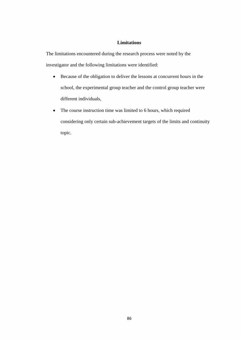
86
Limitations
The limitations encountered during the research process were noted by the
investigator and the following limitations were identified:
Because of the obligation to deliver the lessons at concurrent hours in the
school, the experimental group teacher and the control group teacher were
different individuals,
The course instruction time was limited to 6 hours, which required
considering only certain sub-achievement targets of the limits and continuity
topic.

87
REFERENCES
Aizikovitsh-Udi, E., & Radakovic, N. (2012). Teaching probability by using
GeoGebra dynamic tool and implemanting critical thinking skills.
Procedia-Social and Behavioral Sciences, 46, 4943-4947.
Akkaya, A., Tatar, E., & Kağızmanlı, T. B. (2011). Using dynamic software in
teaching of the symmetry in analytic geometry: The case of Geogebra.
Procedia-Social and Behavioral Sciences, 15, 2540-2544.
Aktümen, M., Yıldız, A., Horzum, T., & Ceylan, T. (2011). İlköğretim matematik
öğretmenlerinin geogebra yazılımının derslerde uygulanabilirliği hakkındaki
görüşleri [Elementary mathematics teachers’ opinions about geogebra
practicality in the lessons]. Turkish Journal of Computer and Mathematics
Education, 2(2), 103-120.
Aktümen, M., Horzum, T., Yıldız, A., & Ceylan, T. (2011). Bir dinamik
matematik yazılımı: Geogebra ve ilköğretim 6-8. sınıf matematik dersleri
için örnek etkinlikler. Retrieved from
http://w3.gazi.edu.tr/web/aktumen/dosyalar/geo gebraturkiye.pdf.
Aktümen, M., & Kaçar, A. (2003). İlköğretim 8. sınıflarda harfli ifadelerle
işlemlerin öğretiminde bilgisayar destekli öğretimin rolü ve bilgisayar
destekli öğretim üzerine öğrenci görüşlerinin değerlendirilmesi [The role of
computer assisted instruction in the teaching of expressions among primary
education eight grade students and evaluation students’ opinion about
computer assisted instruction]. Kastamonu Eğitim Dergisi, 11(2), 339-358.
Aktümen, M., & Kaçar, A. (2008). Bilgisayar cebiri sistemlerinin matematiğe
yönelik tutuma etkisi [Effects of computer algebra systems on attitudes

88
towards mathematics]. Hacettepe Üniversitesi Eğitim Fakültesi Dergisi, 35,
13-26.
Aktümen, M., & Kabaca, T. (2012). Exploring the mathematical model of the
thumbaround motion by Geogebra. Technology, Knowledge and Learning,
17(3), 109-114.
Aktümen, M., & Bulut, M. (2013). Teacher candidates’ opinions on real life
problems designed in GeoGebra software. Anthropologist, 16(1-2), 167-176.
Alacacı, C., & McDonald, G. (2012). The impact of technology on high school
mathematics curriculum. Turkish Journal of Computer and Mathematics
Education, 3(1), 21-34.
Almeqdadi, F. (2000). The effect of using geometer’s sketchpad (GSP) on
Jordanian students’ understanding of geometrical concepts. Proceedings of
the International Conference on Technology in Mathematics Education (pp.
163-169). Lebanon.
Arghode, V. (2012). Qualitative and quantitative research: Paradigmatic
differences. Global Education Journal, 2012(4), 155-163.
Artigue, M. (2002). Learning mathematics in a CAS environment: The genesis of
a reflection about instrumentation and the dialectics between technical and
conceptual work. International Journal of Computers for Mathematical
Learning, 7, 245-274.
Bakar, K. A., Tarmizi, R. A., Ayub, A. F. M., & Yunus, A. S. M. (2009). Effect of
utilizing geometer’s sketchpad on performance and mathematical thinking
of secondary mathematics learners: An initial exploration. International
Journal of Education and Information Technologies, 3(1), 20-27.
89
Baki, A. (2001). Bilişim teknolojisi ışığı altında matematik eğitiminin
değerlendirilmesi [Evaluation of mathematics education in the light of
information technology]. Milli Eğitim Dergisi, 149, 26-31.
Baki, A., & Güveli, E. (2008). Evaluation of a web based mathematics teaching
material on the subject of functions. Computers & Education, 51(2), 854-
863.
Baştürk, S., & Dönmez, G. (2011). Mathematics student teachers’ misconceptions
on the limit and continuity concepts. Necatibey Faculty of Education
Electronic Journal of Science and Mathematics Education, 5(1), 225-249.
Baydaş, Ö., Göktaş, Y., & Tatar, E. (2013). The use of GeoGebra with different
perspectives in mathematics teaching. Çukurova University Faculty of
Education Journal, 42(2), 36-50.
Bildiren, A., & Uzun, M. (2007). Üstün yetenekli öğrencilerin belirlenmesine
yönelik bir tanılama yönteminin kullanılabilirliğinin incelenmesi [An
identification study for gifted students]. Pamukkale Üniversitesi Eğitim
Fakültesi Dergisi, 22(2), 31-39.
Blaisdell, R. (2012). Student understanding in the concept of limit in calculus:
How student responses vary depending on question format and type of
representation. In S. Brown, S. Larsen, K. Marrongelle, and M. Oehrtman
(Eds.), Proceedings of the 15th Annual Conference on Research in
Undergraduate Mathematics Education (pp. 348-353). Portland, Oregon.
Bryman, A., & Cramer, D. (2005). Quantitative data analysis with SPSS 12 and
13: A guide for social scientists. London, UK: Routledge.
Brenner, M. E., Mayer, R. E., Moseley, B., Brar, T., Duran, R., Reed, B. S., &
Webb, D. (1997). Learning by understanding: The role of multiple

90
representations in learning algebra. American Educational Research
Journal, 34(4), 663-689.
Bruner, J. S. (1966). Toward a theory of instruction (Vol. 59). Boston, MA:
Harvard University Press.
Bruner, J. S. (1985). Vygotsky: A historical and conceptual perspective. Culture,
communication, and cognition: Vygotskian perspectives, 21-34. Bulut, M., & Bulut, N. (2011). Pre-service teachers ’ usage of dynamic
mathematics software. Educational Technology, 10(4), 294-299.
Caligaris, M. G., Schivo, M. E., & Romiti, M. R. (2015). Calculus & GeoGebra,
an interesting partnership. Procedia-Social and Behavioral Sciences, 174,
1183-1188.
Choi, K. S. (2010). Motivating students in learning mathematics with
GeoGebra. Annals. Computer Science Series, 8(2), 65-76.
Clements, D. H. (2000). From exercises and tasks to problems and projects:
Unique contributions of computers to innovative mathematics
education. The Journal of Mathematical Behavior, 19(1), 9-47.
Cobb, P., Yackel, E., & Wood, T. (1992). A constructivist alternative to the
representational view of mind in mathematics education. Journal for
Research in Mathematics education, 23(1), 2-33.
Corlu, M. S., Burlbaw, L. M., Capraro, R. M., Han, S., & Çorlu, M. A. (2010).
The Ottoman palace school and the man with multiple talents, Matrakçı
Nasuh. Journal of the Korea Society of Mathematical Education Series D:
Research in Mathematical Education, 14(1), 19–31.
91
Çatma, Z., & Corlu, M. S. (2015). How special are teachers of specialized schools?
Assessing self-confidence levels in the technology domain. Eurasia Journal of
Mathematics, Science, and Technology Education.
DeCoster, J. (2009). Effect size calculator [Excel Add-on]. Retrieved from
http://www.stat-help.com
Doerr, H. M., & Zangor, R. (2000). Creating meaning for and with the graphing
calculator. Educational Studies in Mathematics, 41(2), 143-163.
Duda, B. J., Ogolnoksztalcacych, Z. S., & Poland, Z. (2010). Mathematical
creative activity and graphic calculator. International Journal of Technology
in Mathematics Education, 18(1), 3–14.
Duval, R. (2006). A cognitive analysis of problems of comprehension in a
learning of mathematics. Educational studies in mathematics, 61(1-2), 103-
131.
Filiz, M. (2009). Geogebra ve Cabri geometri II dinamik geometri yazılımlarının
web destekli ortamlarda kullanılmasının öğrenci başarısına etkisi [The
effect of using GeoGebra and Cabri Geometry II dynamic geometry
softwares in a web-based setting on students’ achievement] (Unpublished
master’s thesis). Karadeniz Teknik Üniversitesi.
Gagatsis, A., & Elia, I. (2004). The effects of different modes of representation on
mathematical problem solving. In M. Johnsen Hoines & A. Berit Fuglestad
(Eds.), Proceedings of the 28th Conference of the International Group for
the Psychology of Mathematics Education (Vol. 2, pp. 447-454). Bergen,
Norway: Bergen University College.
Goldin, G. A., & Kaput, J. J. (1996). A joint perspective on the idea of
representation in learning and doing mathematics. In L. P. Steffe, P. Mesher,

92
P. Cobb, G. A. Goldin, & B. Greer (Eds.), Theories of mathematical
learning (pp. 397-430). Hillsdale, NJ: Lawrence Erlbaum.
Goldin, G. A. (2008). Perspective on representation in mathematical learning and
problem solving. In L. D. English (Ed.), Handbook of international research
in Mathematics Education, Second Edition (pp. 176-201). New York, NY:
Routledge.
Goldin, G. A. (2014). Mathematical representations. In Encyclopedia of
Mathematics Education (pp. 409-413). Springer Netherlands.
Gülseçen, S., Karataş, E. K., & Koçoğlu, F. Ö. (2012). Can GeoGebra make easier
the understanding of cartesian coordinates? A quantitative study in
Turkey. International Journal on New Trends in Education and Their
Implications, 3(4), 19-29.
Güven, B., & Kosa, T. (2008). The effect of DGS on student mathematics teachers'
spatial visualization skills. The Turkish Online Journal of Educational
Technology, 7(4), 100-107.
Güven, B. (2012). Using dynamic geometry software to improve eight grade
students' understanding of transformation geometry. Australasian Journal of
Educational Technology, 28(2), 364-382.
Heugl, H. (2001). The necessary fundamental algebraic competence in the age of
CAS. Proceedings of the 5th Austrian Center for Didactics of Computer
Algebra Summer Academy. Austria.
Hohenwarter, M., & Jones, K. (2007). Ways of linking geometry and algebra: the
case of GeoGebra. In D. Küchemann (Ed), Proceedings of the British
Society for Research into Learning Mathematics, 27(3), 126-131.
93
Hohenwarter, M., & Lavicza, Z. (2007). Mathematics teacher development with
ICT: Towards an International GeoGebra Institute. In D. Küchemann (Ed),
Proceedings of the British Society for Research into Learning
Mathematics, 27(3), 49-54.
Hohenwarter, M., Lavicza, Z. (2009). The strength of the community : How
GeoGebra can inspire technology integration in mathematics teaching.
Mathematics, Statistics and Operations Research Connections, 9(2), 3-5.
doi: 10.11120/msor.2009.09020003
Hohenwarter, J., Hohenwarter, M., & Lavicza, Z. (2010). Evaluating difficulty
levels of dynamic geometry software tools to enhance teachers’ professional
development. International Journal for Technology in Mathematics
Education, 17(3), 127-134.
Hohenwarter, M., & Lavicza, Z. (2010, ). GeoGebra, its community and future.
Paper presented at the Asian Technology Conference in Mathematics.
Retrieved from http://www.unsam.edu.ar/
Hohenwarter, M., Hohenwarter, J., Kreis, Y., & Lavicza, Z. (2008). Teaching and
learning calculus with free dynamic mathematics software GeoGebra. Paper
presented at the 11th International Congress on Mathematical Education.
Monterrey, Nuevo Leon, Mexico.
Hohenwarter, M., & Fuchs, K. (2004, May). Combination of dynamic geometry,
algebra and calculus in the software system GeoGebra. ZDM Mathematics
Education, 20(70), 1-5.
Huck, S. W. (2011). Reading statistics and research (6th ed.). Boston, MA.
Pearson.

94
Hutkemri & Zakaria, E. (2012). The effect of GeoGebra on students' conceptual
and procedural knowledge of function. Indian Journal of Science and
Technology, 5(12), 3802-3808.
İçel, R. (2011). Bilgisayar destekli öğretimin matematik başarısına etkisi:
GeoGebra örneği [Effect of computer based teaching on students’
mathematics achievements: Example of GeoGebra] (Unpublished master’s
thesis). Selçuk Üniversitesi Eğitim Bilimleri Enstitüsü, Turkey.
İpek, S., & İspir, O. A. (2011). Preservice elementary mathematics teachers'
geometric and algebraic proof process with dynamic geometry
software. Turkish Journal of Computer and Mathematics Education, 2(1),
20-34.
Jones, K. (2000). Providing a foundation for deductive reasoning: Students'
interpretations when using dynamic geometry software and their evolving
mathematical explanations. Educational Studies in Mathematics, 44(1-2),
55-85.
Jones, K. (2001). Learning geometrical concepts using DGS. In K. Irwin (Ed),
Mathematics education research: A catalyst for change (pp. 50-58).
Auckland: University of Auckland.
Kabaca, T. (2006). Limit kavramının öğretiminde bilgisayar cebiri sistemlerinin
etkisi [The effect of computer algebra systems on teaching limit concept]
(Unpublished doctoral dissertation). Gazi Üniversitesi, Ankara, Turkey.
Kabaca, T., Aktümen, M., Aksoy, Y., & Bulut, M. (2010). Matematik
öğretmenlerinin avrasya geogebra toplantısı kapsamında dinamik matematik
yazılımı geogebra ile tanıştırılması ve geogebra hakkındaki görüşleri
[Introducing the in-service mathematics teachers with the dynamic

95
mathematics software GeoGebra and their views about GeoGebra]. Turkish
Journal of Computer and Mathematics Education, 1(2), 148-165.
Kaput, J. J., & Thompson, P. W. (1994). Technology in mathematics education
research: The first 25 years in the JRME. Journal for Research in
Mathematics Education, 25(6), 676-684.
Karakuş, Ö. (2008). Bilgisayar destekli dönüşüm geometrisi öğretiminin öğrenci
erişisine etkisi [The effects on the students’ success of computer based
transformation geometry learning] (Unpublished master’s thesis). The
University of Eskisehir Osmangazi, Eskisehir, Turkey.
Karakuş, F. (2010). Üstün yetenekli çocukların anne babalarının karşılaştıkları
güçlükler [Difficulties that families of gifted students face]. Mersin
Üniversitesi Eğitim Fakültesi Dergisi, 6(1), 127-144.
Kastberg, S., & Leatham, K. (2005). Research on graphing calculators at the
secondary level: Implications for mathematics teacher education.
Contemporary Issues in Technology and Teacher Education, 5(1), 25-37.
Kepceoglu, I. (2010). Geogebra yazılımıyla limit ve süreklilik öğretiminin öğretmen
adaylarının başarısına ve kavramsal öğrenmelerine etkisi [The effect of
teaching limit and continuity with GeoGebra on pre-service teachers’
achievement and conceptual understanding] (Unpublished master’s thesis).
Marmara Üniversitesi, İstanbul, Turkey.
Kidron, I. (2014). Calculus teaching and learning. In S. Lerman (Ed), Encyclopedia
of mathematics education (pp. 69-75). London: Springer.
Kllogjeri, P., & Kllogjeri, Q. (2011). GeoGebra–a very effective tool for teaching
mathematical concepts and properties. In D. Takači (Ed.), Proceedings of the

96
International GeoGebra Conference for Southeast Europe (pp. 90-98). Novi
Sad: Stojkov.
Kortenkamp, U. (1999). Foundations of dynamic geometry (Unpublished doctoral
dissertation). Swiss Federal Institute of Technology Zurih, Switzerland.
Kutluca, T., & Zengin, Y. (2011, September). Belirli integral konusunda dinamik
matematik yazılımı GeoGebra kullanarak çalısma yapraklarının gelistirilmesi
[Developing worksheets for definite integral by using dynamic mathematics
software with GeoGebra]. Paper presented at the 5th international computer &
instructional technologies symposium, Fırat University, Elazığ.
Leikin, R. (2014). Giftedness and high ability in mathematics. In S. Lerman
(Eds.), Encyclopedia of Mathematics Education (pp. 247-251). Springer
Netherlands.
Mainali, B. R., & Key, M. B. (2012). Using dynamic geometry software GeoGebra
in developing countries: A case study of impressions of mathematics teachers in
Nepal. International Journal for Mathematics Teaching and Learning.
Retrieved from http://www.cimt.plymouth.ac.uk/journal/mainali.pdf/
Masteroides, E., & Zachariades, T. (2004). Secondary mathematics teachers’
knowledge concerning the concept of limit and continuity. In M.J. Hoines, &
A.B. Fuglestad (Eds.), Proceedings of the 28th Conference of the International
Group for the Psychology of Mathematics Education (Vol. 4, pp. 481–488).
Bergen: PME.
Mehanovic, S. (2011). The potential and challenges of the use of Dynamic Software
in upper secondary mathematics: Students’ and teachers’ work with integrals in
Geogebra based environments (Unpublished doctoral dissertation). Linköping
University, Sweden.
97
Mitchelmore, M. C., & White, P. (2004). Abstraction in mathematics and
mathematics learning. In M. J. Høines & A. B. Fuglestad (Eds.),
Proceedings of the 28th Conference of the International Group for the
Psychology of Mathematics Education (Vol. 3, pp. 329–336). Bergen,
Norway: Program Committee.
Ministry of National Education [MoNE]. (2005). Ortaöğretim matematik dersi
öğretim programı [Secondary school mathematics curriculum]. Ankara,
Turkey.
Ministry of National Education [MoNE]. (2012). Fatih Project [Webpage]. Retrieved
from http://fatihprojesi.meb.gov.tr/tr/english.php
Ministry of National Education [MoNE]. (2013). Ortaöğretim matematik dersi
öğretim programı [Secondary school mathematics curriculum]. Ankara,
Turkey.
Ministry of National Education [MoNE]. (2009). Strengthening the vocational
education and training system project in Turkey: Gifted and talented children.
Ankara, Turkey.
Moursund, D. (2006, March 30). Computers in education for talented and gifted
students. Eugene , Oregon, United States of America. Retrieved from
http://pages.uoregon.edu/moursund/Books/TAG/TAG.pdf
Mulyono, B. (2010). Traditional teaching about angles compared to an active
learning approach that focuses on students’ skills in seeing, measuring and
reasoning, including the use of dynamic geometry software: Differences in
achievement (Unpublished master’s thesis). Universiteit van Amsterdam,
Netherlands.

98
National Council of Teachers of Mathematics [NCTM]. (2000). Principles and
standards for school mathematics. Reston, VA.
National Council of Teachers of Mathematics [NCTM]. (2003). NCTM program
standards: Programs for initial preparation of mathematics teachers. Reston,
VA: NCTM.
Orimogunje, E. (2011). Pilot Study. Retrieved from
https://tr.scribd.com/doc/56221002/Pilot-Study
Özel, S., Yetkiner, Z.E., & Capraro, R. M. (2008). Technology in K-12 mathematics
classrooms. School Science and Mathematics, 108(2), 80-85.
Özgün-Koca, S. A. (1998). Students' use of representations in mathematics
education. Paper presented at the Annual Meeting of the North American
Chapter of the International Group for the Psychology of Mathematics
Education, Raleigh, NC.
Özgün-Koca, S. A. (2012). An analysis of prospective mathematics teachers' views
on the use of computer algebra systems in algebra instruction in Turkey and in
the United States. Turkish Journal of Computer and Mathematics
Education, 3(1), 1-20.
Özgün-Koca, S. A., & Meagher, M. (2012). Birth of a virtual manipulative. North
American GeoGebra Journal, 1(1), 27-32.
Özmantar, M. F., Akkoç, H., Bingölbali, E., Demir, S., & Ergene, B. (2010). Pre-
service mathematics teachers’ use of multiple representations in technology-rich
environments. Eurasia Journal of Mathematics, Science & Technology
Education, 6(1), 19-36.
Pallant, J. (2001). The SPSS survival manual: A step-by-step guide to data analysis
using SPSS for Windows (version 10). St Leonards, NSW: Allen & Unwin.

99
Panasuk, R. M., & Beyranevand, M. L. (2010). Algebra students’ ability to recognize
multiple representations and achievement. International Journal for
Mathematics Teaching and Learning, 22, 1-22.
Pape, S. J., & Tchoshanov, M. A. (2001). The role of representation(s) in developing
mathematical understanding. Theory into practice, 40(2), 118-127. Pierce, R. (2005). Using CAS to enrich the teaching and learning of mathematics. In
S-C. Chu, H-C. Lew, & W-C. Yang (Eds), Proceedings of the 10th Asian
Conference on Technology in Mathematics (pp. 47-58). Blacksburg, VA:
ATCM Inc.
Pierce, R., Stacey, K. & Barkatsas, A. (2007). A scale for monitoring students'
attitudes to learning mathematics with technology. Computers and Education,
48(2), 285-300.
Reis, Z. A., & Ozdemir, S. (2010). Using Geogebra as an information technology
tool: parabola teaching. Procedia-Social and Behavioral Sciences, 9, 565-572.
Renzulli, J. S. (1986). The three-ring conception of giftedness: A development model
for creative productivity. In R. J. Sternberg, & J. E. Davidson (Eds.),
Conceptions of giftedness (pp. 53-92). New York: Cambridge University Press.
Saab, M. A., (2011). Implementing dynamic geometry software-based constructivist
approach (DGS-CA) in teaching Thales’ Theorem: Impact of students’
achievement, problem solving skills and motivation (Unpublished master’s
thesis). Lebanese American University, Lebanon.
Saha, R. A., Ayub, A. F. M., & Tarmizi, R. A., (2010). The effects of GeoGebra on
mathematics achievement: Enlightening coordinate geometry
learning. Procedia-Social and Behavioral Sciences, 8, 686-693.

100
Schacter, J. (1999). The impact of education technology on student achievement:
What the most current research has to say. Journal of Educating Computing
Research, 20.
Schoenfeld, A. H. (1985). Mathematical problem solving. Orlando, FL: Academic
Press.
Scientific and Technological Research Council of Turkey. (2005). Vizyon 2023
teknoloji öngörü projesi [Vision 2023: Turkey’s national technology foresight
program]. Ankara, Turkey.
Selçik, N., & Bilgici, G. (2011). GeoGebra yazılımının öğrenci başarısına etkisi
[The effect of GeoGebra software on students’ academic achievement].
Kastamonu Egitim Dergisi, 19(3), 913-924.
Shadaan, P., & Eu, L. K. (2013). Effectiveness of using GeoGebra on students’
understanding in learning circles. The Malaysian Online Journal of
Educational Technology, 1(4), 1-11.
Shore, B. (1997). Keeping the conversation going: An interview with Jerome
Bruner. Ethos, 25(1), 7-62.
Subramanian, L. (2005). An investigation of high school geometry
students’proving and logical thinking abilities and the impact of dynamic
geometry software on student performance (Unpublished doctoral
dissertation). University of Central Florida, Florida.
Swan, M. (2008). Designing a multiple representation learning experience in
secondary algebra. Educational Designer, 1(1), 1-17.
Tabachnick, B. G., & Fiedell, L. S. (2007). Using multivariate statistics (5th ed.)
Boston, MA: Allyn and Bacon.

101
Tall, D. (1993). Students’ difficulties in calculus. In C. Gaulin et al. (Eds.),
Proceedings of Working Group 3 on Students’ Difficulties in Calculus, 7th
International Conference on Mathematicaal Education (pp. 13-28). Québec,
Canada.
Tall, D. (1994). A versatile theory of visualisation and simbolisation in
mathematics. Invited plenary lecture at the CIEAIEM Conference,
Toulouse, France.
Tall, D. O., Smith, D., Piez, C. (2008). Technology and calculus. In M. K. Heid &
G. W. Blume (Eds.), Research on technology and the teaching and learning
of mathematics: Research syntheses (Vol. 1, pp. 207-258). Charlotte:
Information Age Publishing.
Taş, M. (2010). Dinamik matematik yazılımı GeoGebra ile eğrisel integrallerin
görselleştirilmesi [Visualization of curvilinear integrals using the dynamic
mathematics software GeoGebra] (Unpublished master’s thesis). Istanbul
University, Turkey.
Tatar, E., Zengin, Y., & Kağızmanlı, T. B. (2013). Dinamik matematik yazılımı ile
etkileşimli tahta teknolojisinin matematik öğretiminde kullanımı [The use of
dynamic mathematics software and interactive whiteboard technology in
mathematics teaching]. Turkish Journal of Computer and Mathematics
Education, 4(2), 104-123.
Teijlingen, E. R., & Hundley, V. (2001). The importance of pilot studies. Social
Research Update, 35, 1-4.
Uzun, P. (2014). GeoGebra ile öğretimin 7.sınıf öğrencilerinin akademik
başarılarına ve geometriye yönelik tutumlarına etkisi [The effect of instruction
with GeoGebra on 7th grade students’ academic achievement and attitudes

102
towards geometry] (Unpublished master’s thesis). Kastamonu University,
Turkey.
Vanatta, R. A., & Fordham, N. (2004). Teacher dispositions as predictors of
classroom technology use. Journal of Research on Technology in Education,
36(3), 253–271.
Wood, K. (2006). Effect of using multiple representations on student success in
solving rational, radical, and absolute value equations and
inequalities (Unpublished doctoral dissertation). University of Victoria,
Canada.
Zengin, Y. (2011). Dinamik matematik yazılımı GeoGebranın öğrencilerin
başarılarına ve tutumlarına etkisi [The effect of dynamic mathematics
software GeoGebra on students’ achievement and attitude] (Unpublished
master’s thesis). Kahramanmaraş Sütçü İmam University, Turkey.
Zengin, Y., Furkan, H., & Kutluca, T. (2012). The effect of dynamic mathematics
software geogebra on student achievement in teaching of trigonometry.
Procedia-Social and Behavioral Sciences, 31, 183-187.

103
APPENDICES
Appendix 1: Limits and continuity readiness test [LCRT]
1)
limitinin değerini hesaplayınız.
2)
limitinin değerini hesaplayınız.
3) ( )
fonksiyonunun için limitini hesaplayınız.
4) ( )
fonksiyonu için ( ) limitinin değerini hesaplayınız.
5) ( ) {
şeklinde verilen fonksiyonu reel sayılarda
sürekli ise n kaçtır? 6, 7 ve 8. soruların doğru olup olmadığını aşağıdaki bilgiyi göze alarak belirtiniz ve
nedenlerini kısaca açıklayınız.
Bir fonksiyonu için ( ) 6)
7)
8)
İfade Doğru/Yanlış Neden
f(1)=1 olmak
zorundadır
O Doğru
O Yanlış
İfade Doğru/Yanlış Neden
f fonksiyonu x=1
noktasında sürekli olmak
zorundadır
O Doğru
O Yanlış
İfade Doğru/Yanlış Neden
f fonksiyonu x=1
noktasında tanımlı olmak
zorundadır.
O Doğru
O Yanlış

104
9,10,11 ve 12. soruları aşağıdaki grafikten yararlanarak cevaplayınız.
9) ( ) =? 10) ( ) =? 11) ( ) fonksiyonu sürekli midir? Neden? 12) ( ) fonksiyonu (0,2) aralığında sürekli midir? Neden?
𝑔: 𝑅 − { } 𝑅

105
Appendix 2: Limits and continuity achievement test [LCAT]
1)
limitinin değerini varsa hesaplayınız. Yoksa nedenini belirtiniz.
2) (
) limitinin değerini hesaplayınız.
3) ( )
fonksiyonunun için limitini hesaplayınız.
4) ( )
fonksiyonu için ( ) limitinin değerini hesaplayınız.
5) {
şeklinde verilen fonksiyonu reel
sayılarda sürekli ise k+n kaçtır?
6, 7 ve 8. soruların doğru olup olmadığını aşağıdaki bilgiyi göze alarak belirtiniz ve
nedenlerini kısaca açıklayınız:
Bir fonksiyonu için ( ) 6)
7)
8)
İfade Doğru/Yanlış Neden
f(1)=0 olmak zorundadır
O Doğru
O Yanlış
İfade Doğru/Yanlış Neden
f fonksiyonu x=1
noktasında sürekli olmak
zorundadır
O Doğru
O Yanlış
İfade Doğru/Yanlış Neden
f fonksiyonu x=1
noktasında tanımlı olmak
zorundadır.
O Doğru
O Yanlış

106
9)
limitinin değeri kaçtır? Neden?
Aşağıdaki 10, 11 ve 12. soruları verilen grafiğe göre cevaplandırınız.
10) Verilen fonksiyonun hangi nokta(lar)da limiti yoktur? Nedenleriyle birlikte
belirtiniz.
11) Verilen fonksiyon hangi nokta(lar)da sürekli değildir? Nedenleriyle birlikte
belirtiniz.
12) Verilen fonksiyon hangi nokta(lar)da tanımsızdır? Nedenleriyle birlikte
belirtiniz.

107
Appendix 3: Mathematics and technology attitude scale [MTAS]
1. I concentrate hard in mathematics. HE Oc Ha U NA
2. I try to answer questions the teacher
asks HE Oc Ha U NA
3. If I make mistakes, I work until I have
corrected them. HE Oc Ha U NA
4. If I can’t do a problem, I keep trying
different ideas. HE Oc Ha U NA
5. I am good at using computers. SD D NS A SA
6. I am good at using things like VCRs,
DVDs, MP3s and mobile phones SD D NS A SA
7. I can fix a lot of computer problems SD D NS A SA
8. I am quick to learn new computer
software needed for school SD D NS A SA
9. I have a mathematical mind. SD D NS A SA
10. I can get good results in mathematics SD D NS A SA
11. I know I can handle difficulties in
mathematics SD D NS A SA
12. I am confident with mathematics SD D NS A SA
13. I am interested to learn new things in
mathematics SD D NS A SA
14. In mathematics you get rewards for
your effort SD D NS A SA
15. Learning mathematics is enjoyable SD D NS A SA
16. I get a sense of satisfaction when I
solve mathematics problems SD D NS A SA
17. I like using DGS for learning
mathematics SD D NS A SA
18. Using DGS is worth the extra effort SD D NS A SA
19. Mathematics is more interesting when
using DGS SD D NS A SA
20. DGS help me learn mathematics better SD D NS A SA
HE: hardly ever Oc: occasionally Ha: about half the time U: usually NA. nearly always
SD: strongly disagree D: disagree NS: not sure A: agree SA: strongly agree

108
Appendix 4: Written permission for LCRT and LCAT

109
Appendix 5: Written permission for MTAS

110
Appendix 6: Written permission of Ministry of National Education [MoNE]

111
Appendix 7: Worksheets
Matematik Dersi Limit Konusu [Mathematics Lesson Limits Concept]
Çalışma Sayfası-1- [Worksheet-1-]
Aşağıda verilen grafikler için istenilen noktalardaki sağdan ve soldan limitleri
bulunuz. Fonksiyonun o noktada limiti var mıdır? Tartışınız. Limit gösterimlerini
kullanarak ifade ediniz. [Find the left and right limits for the given graphs at the
stated x values. Discuss whether there was a limits of the function at that exact x
value. State the limits by using limits notations.]
a) b)
c) ( )
( )

112
Matematik Dersi Limit Konusu [Mathematics Lesson Limits Concept]
Çalışma Sayfası-2- [Worksheet-2-]
Aşağıdaki tabloyu verilen x değerleri için fonksiyon değerlerini bularak doldurunuz.
Grafikleriyle karşılaştırınız. Hesap makinesi kullanabilirsiniz. [Fill out the table
below by finding values of the functions at the given x values. You can use
calculator.]
x=1.9
x=1.99 x=2 x=2.01 x=2.1
x=1.9
x=1.99 x=2 x=2.01 x=2.1
x=2.9
x=2.99 x=3 x=3.01 x=3.1

113
Matematik Dersi Limit Konusu [Mathematics Lesson Limits Concept]
Çalışma Sayfası-3- [Worksheet-3-]
Aşağıdaki test sorularını limit yaklaşımlarını ve limit özelliklerini kullanarak
çözünüz. [Solve the questions below by considering limiting process and limits
properties.]
1)
2)
3)
4)
5)
6)
7)
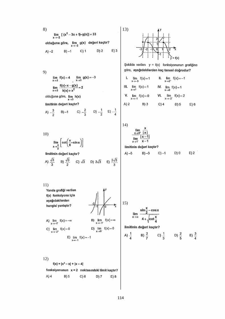
114
8)
13)
9)
10)
11)
12)
14)
15)
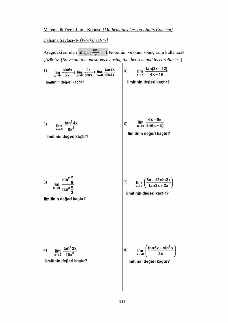
115
Matematik Dersi Limit Konusu [Mathematics Lesson Limits Concept]
Çalışma Sayfası-4- [Worksheet-4-]
Aşağıdaki soruları
teoremini ve onun sonuçlarını kullanarak
çözünüz. [Solve out the questions by using the theorem and its corollaries.]
1)
2)
3)
4)
5)
6)
7)
8)

116
Matematik Dersi Limit Konusu [Mathematics Lesson Limits Concept]
Çalışma Sayfası-5- [Worksheet-5-]
Aşağıdaki soruları çözünüz. [Solve out the questions below.]
1)
2)
3)
4)
5)
6)
7)
8)

117
Matematik Dersi Limit Konusu [Mathematics Lesson Limits Concept]
Çalışma Sayfası-6- [Worksheet-6-]
1)
2)
3)
4)
5) Bir fonksiyon sürekli olduğu her noktada
tanımlı olmak zorunda mıdır? Nedenini
açıklayınız. [Does a function have to be
defined where it is continuous? Explain.]
6) Bir fonksiyon sürekli olduğu her noktada
limitli olmak zorunda mıdır? Nedenini
açıklayınız. [Does a function have limits
where it is continuous? Explain.]
7) Limit konusunun günlük hayatta nasıl
kullanılabileceği konusunda araştırma
yapınız. [Investigate how limits concept
could be used in real life.]
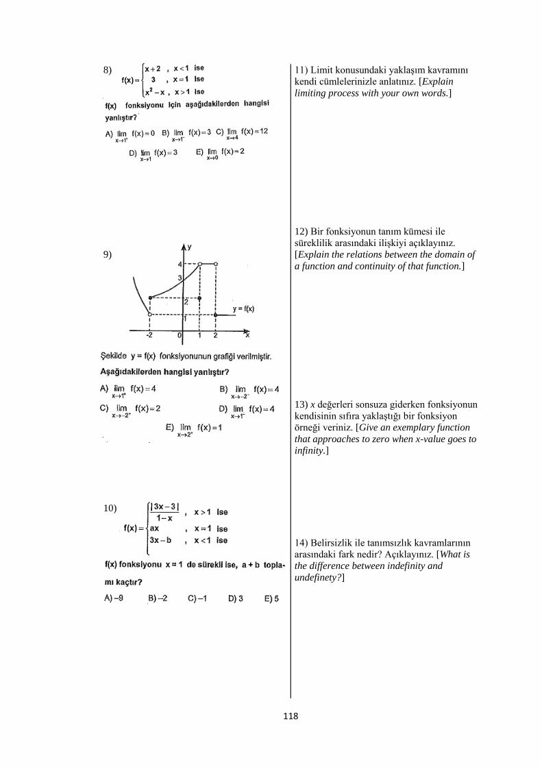
118
8)
9)
10)
11) Limit konusundaki yaklaşım kavramını
kendi cümlelerinizle anlatınız. [Explain
limiting process with your own words.]
12) Bir fonksiyonun tanım kümesi ile
süreklilik arasındaki ilişkiyi açıklayınız.
[Explain the relations between the domain of
a function and continuity of that function.]
13) x değerleri sonsuza giderken fonksiyonun
kendisinin sıfıra yaklaştığı bir fonksiyon
örneği veriniz. [Give an exemplary function
that approaches to zero when x-value goes to
infinity.]
14) Belirsizlik ile tanımsızlık kavramlarının
arasındaki fark nedir? Açıklayınız. [What is
the difference between indefinity and
undefinety?]

119
15)
16)
17)
18)
19)
20)
21)
22)


