Download - The Impact of Public

Economic History Working Papers
No: 331
Economic History Department, London School of Economics and Political Science,
Houghton Street, London, WC2A 2AE, London, UK. T: +44 (0) 20 7955 7084.
The Impact of Public
Transportation and Commuting on
Urban Labour Markets: Evidence
from the New Survey of London
Life and Labour, 1929-32
Andrew Seltzer, Royal Holloway & LSE, and
Jonathan Wadsworth, Royal Holloway
September 2021

1
The Impact of Public Transportation and Commuting on Urban Labour
Markets: Evidence from the New Survey of London Life and Labour,
1929-32
Andrew Seltzer and Jonathan Wadsworth•
Keywords: Commuting, public transport, labour markets, New Survey of
London Life and Labour
JEL codes: N34, N94, J31
Abstract
This paper examines the consequences of the commuter transport
revolution on working class labour markets in 1930s London. The ability
to commute alleviated urban crowding and increased workers’ choice of
potential employers. Using GIS-based data constructed from the New
Survey of London Life and Labour, we examine the extent of commuting
and estimate the earnings returns to commuting. We obtain a lower-
bound estimate of two percent increase in earnings per kilometre
travelled. We also show that commuting was an important contributor
to improving quality of life in the early-twentieth century.
I. Introduction
Urban industry tends to cluster in fairly small geographic areas due to economies
of scale and agglomeration. Prior to the mid-nineteenth century, London was
characterized by workplace concentration with considerable geographic
clustering. Workplace concentration coupled with the inability of workers to
• Please address any correspondence to Andrew Seltzer ([email protected]). We wish to thank
Jessica Bean for discussions early in the project. We also wish to thank Simon Abernathy, Mark
Edele, Rob Gillezeau, Dan Hamermesh, Tim Leunig, Nigel O’Leary, Bruce McClung, and Jens
Wrona for useful comments and suggestions. We have also benefitted from comments from
participants at seminars at Royal Holloway, London School of Economics, University of
Melbourne, University of Swansea, Lund University, the Economic History Society Annual
Conference, Frontier Research in Economic History Conference, the Economic History
Association Annual Conference, the World Congress of Cliometrics, the Australasian and Asian
Society of Labour Economists, Labour Markets and Living Standards in Britain Conference,
Exploring the Breadth of Labour Economics Conference, the World Economic History Congress,
and the Urban History Group. The usual disclaimer applies.

2
commute meant that virtually all workers lived near their place of work (Heblich,
et al 2020). Consequently, the population density of inner London was extremely
high, with some working-class areas, such as the Whitechapel District, containing
over 50,000 residents per square kilometre in the late-nineteenth century (1891
UK Census). Residential concentration created significant negative crowding
externalities in the newly industrialised cities. Much of the debate about the early
Industrial Revolution examines whether the increase in standard of living
associated with higher wages outweighed the costs of higher population density
(Lindert and Williamson 1983; Komlos 1998). However, by the later-nineteenth
and early-twentieth centuries, improved transport, allied to investment in public
housing began to alleviate many of the problems associated with crowding.
Prior to the development of suitable infrastructure, commuting even moderate
distances was infeasible as available forms of travel were slow and expensive. The
commuting revolution began with railways in the mid-nineteenth century (Crafts
and Leunig 2005; Leunig 2006; Heblich, et. al. 2020). By the end of the century,
virtually the entire modern rail Greater London network had been built. Railways
offered a far faster means of transport than anything powered by horses or
humans. However, rail commuting was mostly limited to the middle class and
wealthy well into the twentieth century (Dyos 1982; Polasky 2010). Contemporary
and later accounts generally agree that most working-class Londoners continued
to live very near their workplace into the early-twentieth century (Booth 1902;
Ponsonby and Ruck 1930; Polasky 2010).
Much of the modern bus, tram, and London Underground networks were built in
the early-twentieth century. As we show below, by 1930 virtually all residents
living within about 15 kilometres of the City of London lived within a few hundred
meters of public transport. Unlike the railroads, these transport networks crossed
the central areas, making it possible to commute within the inner boroughs at
relatively high speed and low cost. Buses and trams had near-universal coverage,
with most households in central areas being a fairly short walk away from a stop.
The Underground had its own dedicated tracks, making it considerably faster and

3
more reliable than buses or trams, although it was also more expensive and
geographically limited in coverage. Technological changes, such as the
replacement of horse drawn buses and trams by motorised counterparts, meant
that the speed and availability of public transport increased dramatically in the
early-twentieth century. Concurrently, the average cost per mile travelled
declined sharply between 1900 and 1930.
There is a broad consensus that by the early-twentieth century quality of life was
improving across a range of dimensions (Crafts 1997; Easterlin 2000; Prados de la
Escosura 2015; Chapman 2019). While the existing literature emphasizes the role
of productivity-led increases in income and investment in public health, it is also
plausible that investment in public transport played an important role. The
availability of relatively high-speed, low-cost transport fundamentally altered the
constraint of co-location of workplace and residence. By allowing workers to live
away from their jobs, public transport resulted in net movement away from the
city centre towards the suburbs. This in turn led to a decline in urban crowding.
Urban and labour economists have emphasized a second effect of commuting,
namely increasing the efficiency of labour markets. Competitive theory suggests
that identical workers would be paid identical wages regardless of commute – or
that unobserved worker attributes underlie any difference in earnings. It also
allows for the possibility that employers could pay higher wages to compensate for
attracting workers into a central business district or a remote location (Gibbons
and Machin 2006). Search theory emphasizes that productivity often depends on
the specific match between workers and firms (Mortensen and Pissarides 1994;
Rogerson, et al. 2005). Public transport reduces the travel cost for employees and
thus allows them to search across and commute to more potential employers
(Gibbons and Machin 2006). This, in turn, leads to better matches between
workers and firms.
A second potential labour market effect of improved public transport is a reduction
of employers’ monopsony power (Bhaskar and To 1999; Bhaskar, et. al. 2002,

4
Manning 2003a). Manning (2003b) suggests that acceptable job offers may rise
with distance commuted, so generating a positive relationship between distance
commuted and wages. Workers may also be willing to accept lower wages to avoid
the disutility of longer commuting time. As such, travel costs create a wedge
between net wages (wages less commuting costs) earned at local and distant
employment. This wedge may give employers local monopsony power, as workers’
threat to switch employers is constrained by their commuting costs. Monopsony
power may also derive from differentiated worker preferences over non-wage
attributes across employers. Employers who need large numbers of workers,
particularly non-local workers, will need to offer higher wages. High-speed, low-
cost public transport reduces employers’ monopsony power by reducing the cost to
the worker of commuting to more remote positions paying higher wages.
Our focus in this paper is on the effects of London’s public transport networks on
working-class labour markets, circa 1930. We use data from the New Survey of
London Life and Labour (henceforth New Survey or NSLLL), a household survey
conducted between 1928 and 1932, to examine working-class commuting patterns
and the effects of commuting on earnings. The NSLLL surveyed approximately
two percent of working-class households residing in the 29 Metropolitan Boroughs
and nine adjacent Municipal and County Boroughs. The data contain a range of
personal, housing, and employment-related characteristics. Crucially for our
purposes, the NSLLL provides two indicators of commuting: 1) expenditures per
week on work-related travel and 2) places of residence and work.
We generate GIS coordinates for residences and workplaces, assigning a single
centroid to each unique street address or place name. We also generate GIS
coordinates for the entire rail, Underground, tram, and bus network in the Greater
London area. We use the GIS data to estimate crow-flies distances between
residence, workplace, public transport, and two central points – the Bank of
England (the commercial centre of London) and Charing Cross Station (the
geographic centre of Greater London). These distances provide us with measures

5
of commuting distance, access to public transport, and home and workplace
centrality.
We use these data to examine working-class commuting patterns. Over 70 percent
of workers in the sample had a one-way commute of at least one crow-flies
kilometre. The median (mean) distance was 1.94 (3.05) kilometres. Commuting
followed the expected geographic pattern for a modern metropolis: there were net
flows from outer boroughs to the centre, although there was also a considerable
number of individuals who worked locally or reverse commuted. The wealthy
central boroughs, particularly the ancient centres of Westminster and the City of
London received the largest net commuting inflows.
We also use these distances as independent variables in Mincer-type regressions
on labour force status and earnings. Our results show that the probability of
employment was higher for individuals residing closer to the centre but was not
affected by proximity to public transport. Residing further from the city centre and
living close to an underground station resulted in a greater commuting distance
and higher probability of having transport expenditures. We also find that a one
kilometre increase in distance commuted increased earnings by slightly over two
percent. For a substantial majority of workers in the sample, the monetary return
was greater than the monetary cost of travel. On the other hand, we do not find
particularly large earnings effects for proximity to public transport, although
access to the London Underground indirectly increased earnings through its effect
on distance commuted. These results, particularly the effect of distance commuted
on earnings, are robust to a variety of specifications.
Finally, we compare our results to evidence from the late-nineteenth century.
Booth (1902) provides detailed summary information from the Life and Labour of
the People of London (LLPL), a household survey conducted in the 1890s. Travel
to work was far less of a focus of the LLPL than the NSLLL, suggesting that it
was also a less important aspect of working-class lives. Home-work, the most
extreme form of absence of commuting, was common across a wide range of

6
industries. Few people worked more than a few hundred meters from their
residence (Booth 1902; Ponsonby and Ruck 1930). A simple back-of-the-envelope
calculation shows that approximately one quarter of the increase in working-class
earnings between 1890 and 1930 can be attributed to the effects of increased
commuting distance.
II. Commuting and Labour Markets
Economic theory offers four mechanisms by which lower commuting costs may
increase the efficiency of labour markets. First, lower commuting costs enable
workers to search across more potential employers. Manning (2003b) argues that
the low arrival rate of new job opportunities in a given location is sufficient to
initiate commuting across otherwise identical employers. Workers trade off any
disutility of commuting for higher wages. Mortensen and Pissarides (1994) and
Rogerson, et al. (2005) argue that if there is a match-specific component of
productivity, increased search will lead to better matches between workers and
firms and thus to higher productivity and earnings. Second, lower commuting
costs improves workers’ bargaining position and reduces employers’ local
monopsony power by reducing the gap between net earnings at local and distant
employers (Bhaskar and To 1999; Rotemberg and Saloner 2000; and Bhaskar, et.
al. 2002). Third, workers may distinguish between employers in terms of non-wage
aspects of the job. Because workers differentiate between employers, the labour
supply curve facing individual employers is upward sloping. To attract sufficient
numbers of workers, employers may need to recruit outside their immediate area.
The cost of commuting thus affects individual employers’ labour supply (Bhaskar,
et. al. 2002). Finally, employers who are geographically isolated may need to pay
higher wages as a compensating differential to attract workers. Improvements in
public transport will reduce the cost of travelling to a previously isolated location,
lowering the compensating differential necessary to attract workers (Gibbons and
Machin 2006).

7
Figure 1 shows the relationship between commuting and earnings
diagrammatically. In this framework both workers and jobs are either skilled
(denoted S) or unskilled (denoted U). Skilled jobs pay W0,S and unskilled jobs pay
the lower wage W0,U. Unskilled jobs can be done by either skilled or unskilled
workers, but skilled jobs can only be done by skilled workers. Jobs also differ in
distance from workers’ homes but are homogeneous in terms of other attributes.
The horizontal axis represents physical location, with the worker’s home at the
origin and moves to the right reflecting increasing travel distance. The vertical
axis is the worker’s net wage, e.g. (wage - commuting costs). Commuting costs
include both monetary and time costs; and we assume they increase linearly with
distance travelled in order to simplify the diagram. Finally, we make the
simplifying assumption that workers’ place of residence is exogenously fixed,
deferring the issue of residential choice until Section VI.
The impact of public transport on increased search and better employer/employee
matching can be seen in Figure 1. In the absence of public transport, the net wage
for a skilled worker in a skilled job is shown by WS and the net wage for any worker
in an unskilled job by WU. The gap between WS and WU reflects match-specific
productivity, which occurs when a skilled worker finds a skilled job. Jobs are not
located everywhere, so WS and WU do not show the actual opportunities of workers,
rather the net earnings at all possible locations, conditional on job availability.
The reservation net wages are 𝑊𝑆∗ and, 𝑊𝑈
∗, for skilled and unskilled workers
respectively. If net wages fall below these levels, they choose not to work. We
assume the reservation net wage to be higher for skilled than unskilled workers
(i.e. skilled workers are more productive outside the labour market). A skilled
worker maximizes their net wage by taking the closest available skilled job
between home and l4. If there are no skilled jobs available in this range, they then
compare available skilled jobs between l4 and l5 and unskilled jobs between home
and l0. If there are no unskilled jobs inside l0 or skilled jobs inside l5, they choose
not to work. An unskilled worker maximizes their net wage by taking the closest
unskilled job to their home or, if there are no jobs available inside distance l1, by
not working.

8
Now we consider the effects of building public transport along the space
represented by the horizontal axis. The cost of commuting declines along the
transport route, and thus the net wage curve shifts up. Note that this is direction-
specific, the net wage in other directions does not change. This is shown by the
new wage curves 𝑊𝑈′ and 𝑊𝑆
′. For very short commutes, walking remains less
expensive than public transport, and thus the net wage remains unchanged.
However, for longer travel, public transport reduces the cost of commuting and
thus shifts net wages up. This has two effects on the labour market. First, skilled
workers now earn more than their reservation net wage at skilled jobs between l5
and l6, thus the quality of matches between workers and firms improves. Second,
unskilled workers between l1 and l3 and skilled workers between l0 and l2 now
earn more than their reservation net wage in unskilled jobs, and thus workers
enter the labour force.
A second possible impact of public transport is that it may reduce local monopsony
power (Bhaskar and To 1999; Rotemberg and Saloner 2000; and Bhaskar, et al.
2002). The difference in commuting cost between a nearby employer and a more
distant alternative gives local employers bargaining power. Employers with
perfect information about employees’ outside opportunities will be able to set
wages at less than marginal revenue product, so long as net wages remain above
the worker’s next best alternative. This can be seen in Figure 1. Consider an
employee working immediately adjacent to their home with the next closest
employer is located at lY. In a competitive market, the employee would be paid
W0,S, their marginal revenue product. However, in the absence of public transport,
their outside opportunity is WY. A perfectly price discriminating monopsonist
could pay just above the lower wage WY and still retain the worker. The effect of
public transport is to lower the cost of commuting and thus increase net earnings
at more distant employers. In Figure 1, building high speed public transport along
the horizontal axis shifts the net wage curve up to 𝑊𝑈′ and 𝑊𝑆
′. The skilled worker’s
outside option is now 𝑊𝑌′, and the local employer must pay at least this amount to
retain them. The skilled worker does not switch employers or use public transport,
but is now paid a higher wage due to their increased bargaining power.

9
A third possible impact of commuting (not shown in Figure 1) results from workers
differentiating between employers based on non-wage characteristics. If
employers are sufficiently heterogeneous, they will not be close substitutes for
each other and thus the labour market will not be perfectly competitive (Baskar,
et. al. 2002). Under this sort of monopsonistic competition, individual employers
will face upward sloping labour supply curves. Larger firms would have to pay
higher wages and also to recruit more remotely in order to attract sufficient
workers. If firms can differentiate between employees, they will pay higher wages
only to the marginal employees – those who commute greater distances or face
higher commuting costs. If differentiation is not possible, larger firms will have to
pay higher wages than otherwise equivalent smaller firms in order to recruit
remote workers. Even in this case aggregate wages will be correlated with
commuting distance because larger firms will recruit from further afield.
Monopsony theories can also explain the apparent paradox of ostensibly identical
workers commuting in different directions. If vacancies are hard to find, workers
may have to search for employment in different areas (Manning (2003).
A fourth possible impact of public transport (which is also not shown in Figure 1)
is that it reduces employers’ isolation (Gibbons and Machin 2006). Employers will
locate in areas that are distant from their potential labour force if these areas offer
lower rents, access to raw materials, better distribution networks, etc. However,
isolated firms will be less attractive to workers because of higher commuting costs.
To attract workers these firms will need to increase wages to the point where they
offset these costs; in other words, they need to pay higher wages as a compensating
differential. Improved public transport reduces the cost of commuting to distant
locations and thus reduces the size of this compensating differential.
III. Historical Background: The London Metropolis and Its Commuting
Infrastructure
London is a bicentric metropolis with a commercial centre in the City of London
and a geographic and political centre in the nearby Metropolitan Borough of

10
Westminster. Urban settlement beyond these centres dates back centuries, but
accelerated after the rapid increase in population following the Industrial
Revolution. Settlement outside the centres occurred in every direction. However,
areas north of the River Thames and west of the city centre tended to be wealthier
than areas south and east due to the prevailing winds and river flow.
During the period of our study London was administered under the London
Government Act, 1899. Under the Act, Greater London was divided into the City
of London, 29 Metropolitan Boroughs in the County of London, and a ring of outer
boroughs (officially County Boroughs, Municipal Boroughs, and Urban Districts).1
Following Ponsonby and Ruck (1930), we classify the 38 Boroughs in the New
Survey into central, middle, and exterior rings.2
The New Survey area comprised 429.9 square kilometres, about 27 percent of the
total area of Greater London. It was the most densely populated part of the
metropolis, with about 5,686,000 residents in 1928, approximately 72.4 percent of
the total population of the Greater London area.3 Within the New Survey area,
population density tended to be highest near the centre.4 It is likely that
predominantly working-class areas surveyed in the New Survey contained much
higher population densities than those reported above.5
1 The London Government Act, 1899 was replaced by the LGA, 1963, which abolished the County
of London and restructured the Metropolitan, Municipal, County Boroughs and Urban Districts
into much larger London Boroughs. Throughout this paper we refer to Boroughs and Urban
Districts as of the time of the New Survey. 2 The central boroughs are Bermondsey, Bethnal Green, City of London, Finsbury, Holborn, St.
Marylebone, St. Pancras, Shoreditch, Southwark, Stepney, and Westminster. The middle boroughs
are Battersea, Chelsea, Islington, Kensington, Lambeth, and Paddington. The exterior boroughs
are Camberwell, Deptford, Fulham, Greenwich, Hackney, Hammersmith, Hampstead, Lewisham,
Stoke Newington, Poplar, Wandsworth, Woolwich, and the outer boroughs. The exact location of
the individual boroughs can be seen in Figures 3 and 4. 3 UK Census data, reprinted in London Statistics and Llewellyn-Smith (1930a). 4 The population densities per square kilometre in 1931 were 2303.2, 2127.1, 1007.0, 1323.7, and
499.3 for the central ring, middle ring, exterior ring, New Survey area, and Greater London,
respectively (London Statistics). 5 We are unaware of data on population density for levels below Metropolitan Boroughs. However,
one of the initial reasons for undertaking the both the LLPL and NSLLL was a perception of
widespread crowding in these areas (Booth 1902; Llewellyn-Smith 1930a). It is clear from the
summary volumes of both surveys that working-class dwellings were small, often crowded, and
located close together (Booth 1902; Llewellyn-Smith 1930b). The NSLLL data also show that
approximately 7.7 percent of households and 12 percent individuals lived in crowded households,

11
As with most modern cities, London was characterised by economies of
agglomeration and a resulting industrial concentration. Textiles, furniture-
making, and box-making were heavily concentrated in the East End; the docks
were located by the rivers and major canals; banking, finance, and insurance and
their associated clerical employment were concentrated centrally in the City of
London. To examine population and employment densities more formally, we have
constructed spatial Herfindahl indexes.6 The New Survey area contains 36
residential boroughs and 37 employment boroughs (including the City of London),
and thus a uniform distribution of residences (places of employment) would imply
a residential (workplace) Herfindahl index of .027 (.028).
Table 1 shows the estimated indexes for residences, overall employment, and
employment in the largest 13 industries. The index for overall employment, 0.038,
is slightly higher than for residences, 0.035, which is itself somewhat higher than
if residences were uniformly distributed across boroughs. While these numbers
seem fairly small relative to the baseline of 0.027, they reflect considerable
concentration. The residential index of 0.035 reflects the fact that there are
approximately 9.1 times as many observations in the New Survey data (6,958 vs
763) in the largest residential borough (Islington) as the smallest (Chelsea). The
degree of spatial concentration by industry varied considerably. Financial services
and “footloose” industries – such as construction, painting, and metal working –
had similar levels of spatial concentration to residences. Personal services,
transport and communications, and some manufacturing industries (typically
those dominated by small firms) had higher levels of spatial concentration.
Clerical work and printing had substantially higher levels of spatial concentration.
It can also be seen in Table 1 (column 2) that the largest share of employment for
most industries was in one of the central boroughs.
defined as more than two people to a room (Llewellyn-Smith 1930b; Hatton and Bailey 1998). If
crowding is defined by the so-called Manchester standard of over 2.5 individuals to a bedroom
(Llewellyn-Smith 1930b), approximately 34.7 percent of households and 46.4 percent of individuals
lived in crowded conditions. 6 Formally, the index is given by ∑ 𝑆𝐵
2𝑁𝐵=1 where SB denotes the share of the population residing or
employed in borough B. We exclude workplace observations from Tottenham, Walthamstow, and
outside the New Survey area when calculating workplace indexes.

12
The concentration of employment in central areas meant that commuting to work
was necessary to prevent over-crowding. However, travel was slow until the mid-
nineteenth century. Walking averaged at most five kilometres per hour, and
probably somewhat less.7 The only faster alternative was horse-drawn hackney
carriages (and horse-drawn omnibuses and trams from 1829 and 1861,
respectively), which averaged 6-10 kilometres per hour, but were beyond the
means of but the very wealthy (London Transport Museum 2020). Consequently,
up to the mid-nineteenth century virtually all workers lived nearby their place of
employment (Heblich, et. al. 2020). The development of the faster transport
infrastructure needed for longer-distance commutes occurred from the mid-
nineteenth through the early-twentieth centuries. Table 2 shows some statistics
on speed, coverage, cost, and usage of railways, the London Underground, trams,
and omnibuses in 1900-07, 1913, and 1929. The dramatic improvements in public
transport shown in Table 2 led to an increase in usage, which far outpaced the
population growth over the same period of time.
Railways were first built in London in 1836. The rail network expanded rapidly,
and most of the modern network was complete by the end of the nineteenth
century. Compared to other available means of transport, trains were fast. In
1907, the average scheduled speed for commuting trains into central London
terminal stations was about 32.3 kilometres an hour (Statistics London, 1907).8
The availability of fast transport led to the growth of middle-class residential
suburbs. The pattern of residential movement away from the centre is particularly
evident for the City of London, which experienced a dramatic decline in residential
7 Five kilometres per hour is a widely cited average walking speed first proposed by the Scottish
mountaineer William Naismith. However, Naismith’s rule assumes level ground, no
encumbrances, and no stoppages; and thus urban walking speed was probably substantially
slower. We follow Leunig (2006) and assume a walking speed of 4.0 kilometres an hour throughout
this paper. 8 London Statistics (1907) shows the inward speed for 20 suburban train routes with terminus at
a central London station between 8:00 and 9:00 am. The figure of 32.3 kilometres per hour is the
average across these routes, weighted by the number of trains on each route. This figure is
consistent with other sources. Leunig (2006) uses surviving train timetables and calculates that
the scheduled rail speed for “minor journeys” (inner-city routes with many stops to provide local
service) were 30.4 and 32.8 kilometres per hour in 1887 and 1910, respectively.

13
population from 130,117 in 1801, to 43,882 in 1891, and 15,758 in 1931 (UK
Census), although employment continued to grow over this period.9
Figure 2, panel A, shows the railway network circa 1930 and the borders of the
County of London and the New Survey area. The map of the network shows two
important features of rail travel. First, there was extensive coverage of the exterior
of the Greater London area. Virtually all built up locations within the area were
connected to the centre by rail. Second, rail commuting across the central areas of
the City of London and Westminster was much more difficult, as the terminal
stations of the network were built on what was the outskirts of the central area
when the rail networks were first built in the mid-nineteenth century.10 There
were few direct connections between the terminal stations. These two
characteristics meant that rail travel was typically used for longer-distance
commutes from the suburbs to the centre or, less frequently, reverse commuting
out from the centre to industrial suburbs.
Although rail commuting transformed the lives of the wealthy and middle classes,
most scholars have argued that, with the exception of a relatively small number
of relatively high earners, few working-class employees commuted by rail in the
nineteenth century.11 Ponsonby and Ruck (1930) argue that even circa 1930, rail
was a relatively infrequent mode of commuting for the working-class, typically
9 The City of London undertook Day Censuses in 1866, 1881, 1891, and 1911 to demonstrate its
continued commercial importance. The Reports of the Day Censuses show that many non-residents
entered the City every day and that employment increased substantially even as the residential
population declined. The estimated daytime population of the City of London was 261,061 in 1881;
301,384 in 1891; 364,061 in 1911; and 436,721 in 1921 (Day Census, 1881-1911 and UK Census,
1921). Table 1 shows that the City of London remained the largest employment location at the time
of the New Survey. 10 The opening of the Metropolitan Underground Line in 1863 provided limited connections
between the terminal rail stations and the central areas of London. However, coverage was limited
and additional ticket cost would have been beyond the means of most working-class employees in
the late-nineteenth century. 11 See Ponsonby and Ruck (1930), Dyos (1953), Polasky (2010). Even into the twentieth century,
rail commuting from the outer boroughs was not practical for most working-class households.
These households often had multiple earners, thereby would have required multiple fares. Working
class employees also worked very long hours and thus faced time constraints and faced sufficiently
irregular employment that many could not be sure of work when they would have had to board a
train (Booth 1902; Maddison 1964; Huberman and Minns 2007).

14
used for very long commutes (over 16.1 kilometres) or as a substitute for the
Underground in the south and east of the metropolis.
Working-class access to public transport did, however, improve dramatically in the
early-twentieth century. New modes of transport made it practical to commute
between inner-city locations. New infrastructure and technology, most notably the
development of the Underground network and the replacement of horse-drawn
buses and trams by their motorised counterparts, reduced the cost and increased
the speed and reliability of travel. Buses and trams were cheap, with fares starting
at ½d, whereas Underground fares were typically 2d or more.12 The Underground
lines, trams, and buses were owned separately, but were regulated under a
common framework established under the London Traffic Act of 1924. Public
transport companies sometimes competed for passengers on the same route until
their consolidation under the London Passenger Transport Act and the formation
of the London Transport Board in 1933.13
Although its first underground train line was opened in 1863, the core of the
modern Underground network was built in the early twentieth century. The
Central London Railway (the Central Line), Baker Street & Waterloo Railway (the
Bakerloo Line), Piccadilly & Brompton Railway (the Piccadilly Line), and Charing
Cross, Euston & Hampstead Railway (the Northern Line) opened in 1900, 1906,
1906, and 1907, respectively.14 The Underground ran at similar speeds to mainline
rail. However, unlike the rail network, the Underground network was designed to
12 Prices are reported using “old” pounds sterling, where one pound (£) equals 20 shillings (s) and
one shilling equals 12 pence (d). 13 In addition to public transport, bicycles were an important form of transport for the working-
class. Aldred (2014) argues that bicycles were relatively cheaper and much more widely used for
commuting in 1930 than in 1900. It is not possible to determine the exact number of workers
commuting by bicycle, as the New Survey recorded transport expenses rather than mode of
transport. Nevertheless, commuting by bicycle is specifically mentioned for 288 individuals and it
is likely that many individuals with zero or missing commuting expenditures cycled to work.
Private cars and motorcycles were beyond the means of almost all workers in our sample. These
modes of transport are specifically mentioned for only 12 individuals. 14 By 1907 the routes that would become the Central, District, Metropolitan, Central, Bakerloo,
Piccadilly, and Northern Lines were all largely completed. Although the outer termini of these
lines would be extended between 1907 and 1930, no new lines were opened from 1907 until the
opening of the Victoria Line in 1969.

15
cross the inner city, and made it feasible to commute between most locations in
the north and west regions of the NSLLL area. The limiting factor on Underground
usage was its cost, with 58 percent of journeys in 1930 costing 2d or more
(Ponsonby and Ruck 1930, p. 187). While the average fare per mile on the
Underground was lower than the bus or tram (Table 2), the Underground was
more expensive for shorter journeys. Ponsonby and Ruck (1930) argue that circa
1930 the Underground was the primary mode of working-class travel for distances
between 3.2 and 19.3 kilometres.
Figure 2, panel B shows the Underground network circa 1930. Unlike the rail
network, the Underground network was geographically concentrated, with over 80
percent of stations located north of the River Thames and west of the eastern
boundary of the City of London. This concentration occurred for both geological
and economic reasons. North of the River Thames, the soil is predominantly
“London clay”, which is comparatively easy and inexpensive to tunnel through and
is largely impermeable to water (Paul 2016). In most areas south of the Thames,
the London clay is covered by sand and silt which is porous and difficult to tunnel
through. Even today, virtually all of the deep underground rail network is located
in the areas where the London clay is near the surface. The boroughs east of the
City of London were poorer than those to the west, and the Underground was
generally not extended to this area, regardless of geological suitability.15 The outer
parts of the metropolis, with the exception of a few wealthier areas to the north
and west, were generally not serviced by the Underground because the density of
traffic would not have been sufficient to justify the high initial fixed investment.
Private horse-drawn carriages (or “hackneys”) have been used in London for
centuries. Horse-drawn omnibuses open to the public were first run in 1829
(London Transport Museum 2020). Horse-drawn trams date back to 1860. In the
twentieth century, electric, diesel, and petrol engines replaced horses (London
Transport Museum 2020). Circa 1930, buses and trams were similar in terms of
15 The entire area east of the City of London contained only one Underground line (District) and 9
stations.
16
vehicle design, speed, and cost, with the only major difference being that trams
ran on fixed lines whereas buses could be run on any road (Ponsonby and Ruck
1930; London Transport Museum 2020). Both were substantially slower than rail
or the Underground, but were also cheaper on short routes. Ponsonby and Ruck
(1930) argue that workers used buses and trams interchangeably on journeys of
up to 3.2 kilometres.
The bus and tram networks circa 1930 are shown in Figure 2, panels C and D.
Trams were contained within inner-London, with few routes extending beyond the
boundaries of the New Survey area. Tram density was highest in areas without
Underground lines. On the other hand, buses were the most widely distributed
form of public transport. In 1931 there were 209 routes within Greater London,
covering virtually all built-up areas. Virtually all residents of the New Survey area
had access to at least one bus route, and only a few households in the outer
boroughs were located more than a few hundred meters from a route.
IV. Data
Our primary source of data are records from the New Survey of London Life and
Labour, a household survey of working-class residents of the 29 Metropolitan
Boroughs and nine outer boroughs conducted between 1928 and 1932. Most of the
original record cards have survived intact, and were encoded in the 1990s by the
team of Roy Bailey, Dudley Baines, Timothy Hatton, Paul Johnson, Anna Leith,
and Angela Raspin. The original cards from the Municipal Boroughs of
Walthamstow and Tottenham, the two northernmost boroughs in the sample, have
been lost.16 The computerized records are freely available from the UK Data
Archive (Johnson, et. al. 1999). The computerized records contain 26,915
households, 94,137 individuals, and 49,445 income earners, about two percent of
the working-class population of London.
16 The adjacent boroughs of Leyton and Hornsey comprise slightly over 3 percent of the NSLLL
sample and thus it is likely that the share of records lost was fairly small.

17
The NSLLL was created to follow the LLPL, which influences both the sample and
the questions. The LLPL surveyed residents of the 29 Metropolitan Boroughs,
excluding the City of London, which had few working-class residents by the 1890s.
The NSLLL also included the County of London (again excluding the City of
London). However, by the late-1920s there had been outward movement of
working-class residences, thus the NSLLL also included nine adjacent outer
boroughs.17
The sample is limited to working-class households, defined by the head of
household not working in a white-collar occupation. Most households surveyed
earned well below £250, approximately the median household income in London
in 1929. The mean (median) wage earnings for households with at least one income
earner was £110/14s/5d (£100) and only 7.5 percent of households in the sample
earned more than £200.18
The NSLLL was structured by individual household. Each record card contains
background information about each member of the household: age, gender, place
of birth (for adults), relation to head of household, and different sources of non-
wage income. The cards also contain information on the dwelling: address;
borough; rent paid; number of bedrooms; and whether it contains a kitchen,
pantry, scullery or larder, bath, parlour, garden, yard, and allotment. Finally, they
contain the following additional information for each working member of the
household: earnings in the previous week and in a full-time week, hours worked
in the previous week and in a full-time week, occupation, employer, place of work,
and transport expenditures. A complete list of the information on the record cards
17 These were Acton, Barking, East Ham, Hornsey, Leyton, Tottenham, Walthamstow, West Ham,
and Willesden. These boroughs contained the majority of working-class residents of the Greater
London area outside the County of London (Llewellyn-Smith 1930a). 18 These figures likely overestimate annual earnings, which we estimate using the standard
approach of multiplying pay in a full week by 50 weeks. Some intermittent employment was for
less than 50 full-time weeks per year. A rough indication of the extent of intermittency can be
obtained by comparing hours worked in the previous week and hours worked in a full -time week.
Approximately one percent of those reporting positive hours in a full-time week also reported zero
hours in the previous week. Hours worked in the previous week is missing for another 2.5 percent.
Approximately 7.0 percent of workers reported working less than full time hours in the previous
week, compared to only about 1.0 percent who reported working more than full time.

18
is shown in Appendix I. Summary statistics for variables used in the paper are
shown in Appendix I, Table A.I.1.
For our purposes, the most important feature of the data is that it contains
information about travel to work. The only direct information in the data is
expenditure on transport. However, using transport expenditure to measure
commuting is problematic for our purposes. This information is missing for about
30.8 percent of workers who worked a positive number of hours in the previous
week.19 In addition, many respondents did not supply easily quantifiable answers
to the question about transport expenditures, e.g. “bicycle” or “it varies”. Moreover,
it is possible that some non-commuting-related travel costs are included in the
responses even though the question was clearly intended to cover commuting costs
only (see Appendix I). Finally, the monetary cost of travel does not incorporate the
implicit costs of workers’ time commuting and thus would not reflect the full cost
of transport even absent errors in the data. For these reasons, we only use
transport expenditures for robustness tests, rather than as the main indicator of
commuting in our analysis.
As an alternative to travel expenditure, we measure the crow-flies distances
between individuals’ residence and workplace, residence (workplace) and the
geographic and commercial centres of London, and residence (workplace) and
nearest available public transport. To do this, we first generate GIS coordinates
for each relevant point of interest using Streetmap.co.uk and National Library of
Scotland (2020). For each unique location we generate GIS coordinates for a single
centroid, typically at the centre of each street or place name. In addition to home
and workplace, we have gathered GIS data for the entire public transport network
within the Greater London area. We then used the GIS coordinates and the Great
Circle Distance formula to construct several variables measuring crow-flies
19 When coding transport costs, we have handled missing observations in two ways. First, we
simply leave these as missing and drop the observations from the analysis. Secondly, we recode
missing values to zero if the individual’s residence and workplace were less than a kilometre apart.
We generally prefer the second approach, as one kilometre is a plausible walking distance and
virtually no individuals in the data residing within a kilometre of their workplace reported non-
zero transport costs.

19
distances between home, workplace, the nearest public transport, and the nearest
centre of London. Appendix II outlines in detail the procedures used to obtain the
GIS data and construct the distance variables and the potential sources of
measurement error and bias in these variables.
V. Summary Statistics on Commuting
Table 3 shows some summary statistics on distances.20 The first 8 rows show the
mean distances from home and then workplace to the nearest available point of
embarkation for each of the four modes of public transport. As would be expected
based on Figure 2, the average distance from both home and work is largest for
the Underground and smallest for buses. The variance is also much higher for the
Underground, due to its incomplete coverage. Table 3 also shows the universality
of access to at least some form of public transport. A household two standard
deviations above the mean distance from the nearest bus stop, would nevertheless
still be in easy walking distance of a stop (520 meters). Only 0.02 percent of income
earners in the sample resided more than one kilometre from the nearest available
means of public transport.
The next 15 rows of Table 3 show the distribution of crow-flies distances between
home and work. The mean and median distances were 3.05 and 1.94 kilometres,
respectively; less than modern commutes, but considerably more than “working
on the spot”, which was typical in the 1890s (Ponsonby and Ruck 1930).21 It is also
evident that on average 1) men commuted greater distances than women, 2)
commuting distance increased with skill, and 3) commuting distance was very
similar for heads of households and others. The construction of the sample implies
that it is likely that the average commute across the entire London population was
20 Approximately eight percent of workers who report pay were itinerant, with no fixed place of
work. We did not assign a commuting distance to these workers. See Appendix II for further
details. 21 According to figures from the 2011 UK Census, the average commute for full-time workers in
Greater London was 16.4 kilometres (Greater London Authority 2015). The New Survey area
comprises the central-most part of Greater London, thus one would expect shorter average
commutes than for the Metropolis as a whole.

20
almost certainly greater than shown in Table 3 because the NSLLL sample only
includes workers who lived relatively close to the centre.
The final four rows show the direction of commuting, divided into four mutually
exclusive and collectively exhaustive categories: inwards – workplace is at least
one kilometre closer to the centre than home, outwards – home is at least one
kilometre closer to the centre than workplace, local – distance travelled is less
than one kilometre, and across – distance travelled is at least one kilometre but
there is less than one kilometre difference in home and workplace centrality. The
largest share, (38%), commuted inward, followed by working locally, (29%), but
around one third of workers in the sample commuted outward or across London.
Figures 3 and 4 explore the patterns of commuting by borough of residence and
workplace. Figure 3 shows the workplaces for residents of four boroughs: Stepney
(an East End borough adjacent to the City), Lambeth (a largely working-class
borough which runs from directly across the river from the City to the southern
boundary of the New Survey area), Westminster (the political and geographic
centre of the metropolis), and Islington (an inner-north borough with the largest
working-class population in the metropolis).22 Figure 4 shows net commuting
inflows and outflows by borough of residence.
The conclusions from Figures 3 and 4 are fairly consistent, and we summarize
them jointly. The general pattern across all residential boroughs was that the
largest share of workers either worked within their borough of residence or
commuted inwards to the centre. Consistent with evidence from earlier Day
Censuses and the 1921 UK Census, the City of London was the largest net recipient
of commuters, although the wealthier boroughs north and west of the City were
also net recipients. The exterior boroughs were typically “dormitory suburbs”,
although some had large employers that attracted many workers from other
22 We have constructed similar figures for each of the 36 residential boroughs in the data. This is
shown in Appendix IV, Figure A.IV.1. The patterns shown in Figure 4 are common across the
remaining boroughs.

21
boroughs, such as the Arsenal at Woolwich or the docks at Bermondsey and
Poplar.
VI. Empirical results
i. Estimation Strategy
The models outlined in Section II imply that proximity to and use of public
transport will have direct effects on labour markets. Proximity to public transport
reduces the (time) cost of commuting. This in turn leads to a higher likelihood of
using public transport and longer commutes, which may lead to higher income
through the mechanisms outlined in Section II. In this section, we examine the
impact of public transport and commuting using the New Survey data, augmented
by the GIS data described in previous sections.
To examine labour force status, we run probit regressions of the general form:
𝐸𝑀𝑃i = 𝑎 + 𝐵𝑋𝑖 + 𝑏2𝐷𝐶𝐸𝑁𝑇𝐻,𝑖 + 𝑏3 𝐷𝑈𝐻,𝑖 + 𝑏4𝐷𝑇𝑟𝑎𝑖𝑛𝐻, 𝑖 + 𝑏5 𝐷𝑇𝑟𝑎𝑚,𝐻 𝑖 + 𝑏6𝑗 𝐷𝐵𝑢𝑠𝐻,𝑖 + 𝑒𝑖
where:
EMP is a dummy variable taking a value of one if an individual is employed.
We define employment as either having an earner number or reporting non-
zero working hours in the previous week.
X – control variables: age, age2, age not reported, age > 14 (the school-leaving
age in 1930), sex, born in England, born in London, born in same borough as
current residence, born in an adjacent borough to current borough of
residence, wage income of other family members, non-wage income of the
household, and borough of residence.
DU,H – crow flies distance (CFD) home to nearest underground station.
𝐷𝑇𝑟𝑎𝑖𝑛,𝐻 – CFD home to nearest train station.
𝐷𝑇𝑟𝑎𝑚,𝐻 – CFD home to nearest tram stop.
𝐷𝐵𝑈𝑆 – CFD to nearest bus stop.
DCENT,H – MIN[CFD home to Charing Cross, CFD home to Bank of England].
To examine distance commuted or use of public transport we run the following
regressions:

22
𝐶𝑂𝑀𝑖 = 𝑎 + 𝐵𝑋𝑖 + 𝑏2𝐷𝐶𝐸𝑁𝑇𝐻,𝑖 + 𝑏3 𝐷𝑈𝐻,𝑖 + 𝑏4 𝐷𝑇𝑟𝑎𝑖𝑛𝐻, 𝑖 + 𝑏5 𝐷𝑇𝑟𝑎𝑚𝐻 𝑖 + 𝑏6𝑗 𝐷𝐵𝑢𝑠𝐻 ,𝑖 + 𝑒𝑖
where:
COM – is a variable indicating the extent of commuting. We define this in
several ways: crow-flies distance commuted, whether reporting positive
commuting expenditures, whether distance commuted was less than one
kilometre, and whether distance commuted was 3.2 kilometres or more.23
X – control variables: age, age2, age not reported, sex, hours worked last
week, hours worked not reported, born in England, born in London, born in
same borough as current residence, born in an adjacent borough to current
borough of residence, and borough.
To address the impact of commuting on earnings, we run modified Mincer-type
wage regressions (Mincer, 1958 and 1974) of the general form:
ln(𝑃𝑎𝑦𝑖) = 𝑎 + 𝐵𝑋𝑖 + 𝑏1𝐷𝐸,𝑖 + 𝑏2𝐷𝐶𝐸𝑁𝑇𝐻,𝑖 + 𝑏3 𝐷𝑈𝐻,𝑖 + 𝑏4 𝐷𝑇𝑟𝑎𝑖𝑛𝐻, 𝑖 + 𝑏5 𝐷𝑇𝑟𝑎𝑚,𝐻 𝑖
+ 𝑏6𝑗 𝐷𝐵𝑢𝑠𝐻,𝑖 + 𝑏2𝐷𝐶𝐸𝑁𝑇𝑊,𝑖 + 𝑏3 𝐷𝑈𝑊,𝑖 + 𝑏4𝐷𝑇𝑟𝑎𝑖𝑛𝑊, 𝑖 + 𝑏5 𝐷𝑇𝑟𝑎𝑚𝑊, 𝑖
+ 𝑏6𝑗 𝐷𝐵𝑢𝑠𝑊 ,𝑖 + 𝑒𝑖
where:
Pay – earnings in the previous week in hundredths of old pence.
X – control variables: age, age2, age not reported, sex, hours worked last
week, hours worked not reported, born in England, born in London, born in
same borough as current residence, born in an adjacent borough to current
borough of residence, skill level, occupation, and boroughs of residence and
workplace.
H, W subscripts denote home and workplace, respectively.
The frameworks outlined in Section II imply the following for the regression
coefficients. Living close to one of the centres implies a higher density of local jobs
and lower commuting costs needed to reach a suitable job. Thus, we expect
residential centrality to be associated with a higher likelihood of being employed,
a lower likelihood of commuting by public transport, and shorter commutes.
Proximity to public transport will reduce the (non-monetary) cost of its usage.
23 The cut-off points of 1.0 and 3.2 kilometres are selected based on discussion about transport
mode in Ponsonby and Ruck (1930). In the data, 92.1 percent of workers with reported
expenditures who commuted less than 1.0 kilometres reported expenditures of exactly zero.
Among workers with non-missing expenditures commuting over 3.2 kilometres, 89.8 percent
reported positive transport expenditures.

23
Thus, we expect it to be associated with a higher probability of employment and a
higher probability of positive transport expenditures.
The effect of proximity on distance commuted is likely to vary across the different
modes of public transport. Workers typically used buses or trams for short
distances, and trains or the Underground for longer distances (Ponsonby and Ruck
1930). A worker residing nearby a bus or tram would be more likely to use these
modes of transport than to walk and thus commute further, but also more likely
to use them instead of trains or the Underground and thus have a shorter
commute. By a similar line of reasoning, proximity to trains or the Underground
would lead to longer commutes for those who use public transport. However,
stations, particularly the larger train stations, were themselves important focal
points of local employment. This implies an ambiguous relationship between
residential access to trains or the Underground and commuting distance. Finally,
the frameworks described in Section II imply that greater residential access to
public transport, greater commuting distance, and lower workplace access to
public transport will all result in higher earnings.
ii. Endogeneity of Location
An important econometric issue associated with these regressions is that the
locations of both residence and workplace are choice variables and thus there
exists the possibility of reverse causality in an OLS regression on the full sample.
Income may determine commuting distance by affecting the set of available
residential choices. Put simply, a high earning individual could choose to live
either near their workplace or alternatively in distant residential suburbs and
commute into work. The existence of reverse causation would imply that the
estimated coefficients on the distance variables in an OLS regression would be
biased, and a priori the direction of the bias is ambiguous. Llewellyn-Smith
(1930b) argues that London housing rental markets were very tight circa 1930,
and respondents in the NSLLL would not have had the extent of residential choice
that would be open to Londoners today. Nevertheless, it is very likely that there
24
was at least some degree of residential choice, and it is necessary to mitigate the
associated potential biases.
The standard approach to identification with this sort of endogeneity concern
would be to use an instrumental variable (IV). However, it is far from clear that
the cross-sectional NSLLL data (Appendix I) contains a suitable instrument which
will satisfy both of the required exclusion restrictions: e.g. relevance (the
instrument must be correlated with the distance variables) and exogeneity (the
instrument cannot plausibly directly influence the dependent variable through
mechanisms other than its correlation with the distance variables).
Because the standard IV approach is not viable, we have attempted to limit the
extent of endogeneity in other ways. First, we restrict our sample to individuals
who presumably had the least choice with regard to residential location. There
exists a literature in urban economics which assumes that households’ residential
choices revolve around the primary income earner (Kain 1962; O’Reagan and
Quigley 1993, Rees and Shultz 1970). Thus, our preferred regression specifications
exclude heads of household and non-family members. Non-relatives (such as
lodgers) presumably had the greatest extent of residential choice, and thus these
individuals are also excluded from our preferred regression specification.24
Because we cannot be sure that our approach of restricting the sample fully
mitigates against endogeneity, we have also estimated the regressions splitting
the sample several different ways as a robustness check.
Another strategy that will help control for endogeneity caused by any unobserved
heterogeneity in location choice is to estimate over all individuals in a household
and to include household fixed effects in the estimation. Including household fixed
effects means that the distance variables are identified by within-household
24 Heads of household are defined either by the relationships given on the original record cards or
by the highest earner within the household. We use the relationship categories from the original
record cards to decide whether individuals were related to the head of household. We have
excluded individuals if there is ambiguity in the relationship (“single”, “bachelor”, “spinster”) as
well as if it is clear that they were unrelated (“lodger”).

25
differences in commuting. This will reveal whether individuals in the same
household (and by extension the same location) receive higher wages with distance
travelled. This approach will mitigate against biases associated with any
unobserved characteristics that also determine wages.
iii. Effects of Public Transport on Labour Force Status and Commuting Distance
Table 4 shows results for the employment and distance commuted regressions for
the sample who are related to the head of household and aged 14 or over. The first
two columns show results for the probability of being in work. We report the
estimated marginal effects for the explanatory variables of interest.25 The last five
columns show results for distance commuted. To ensure the robustness of our
results, we change the dependent variable in the different specifications, and, in
column 4, jointly estimate the effects on employment and commuting distance
using the Heckman correction. In this regression, the first stage is identified by
the standard “labour supply” variables, wage income of other family members and
non-wage income of the household.
While the estimated signs of the distance effects are the same for the two
participation specifications, their significance differs. The coefficient on distance
from the nearer centre is negative and significantly different from zero in the
earner number specification, (column 2) but not the hours worked specification,
(column 1). These differences stem from observations with missing hours among
self-employed workers, who typically commuted shorter distances. Individuals
residing more centrally were more likely to be employed, presumably because of
the greater concentration of jobs in the central areas. Closer access to a train
station is negatively associated with the likelihood of being in work in the hours
worked model. Closer access to a bus stop is positively associated with working.26
25 The estimated marginal effects for the other explanatory variables are given in Appendix IV,
Table A.IV.1. 26 As robustness tests we re-estimate the models using family fixed effects (Appendix IV, Table
A.IV.2). We also replaced the distance from public transport variables with the number of
train/Underground stations and bus/tram routes in the same 500 square meter grid (and one
square kilometre grid) as the individual’s residence. The results are qualitatively similar to those
shown in Table 4.

26
The results of the commuting regressions are consistent across specification.
Workers residing near one of the centres commuted shorter distances, (columns 3
& 4, row 1), were less likely to incur transport expenses, (column 5 row 1), were
more likely to work locally, (column 6 row 1) and were less likely to commute
medium to long distances (column 7 row 1). As with the employment regressions,
the logical interpretation of this result is that labour markets were much thicker
and thus there were more local employment opportunities near the two centres.
Access to the Underground – conditional on distance from the centre – was
associated with longer commutes, a higher probability of incurring transport
expenses, a lower probability of working locally, and a higher probability of a
medium to longer commute (row 3, columns 3 to 7). There is a sharp contrast
between access to the Underground and access to the train system, the two
transport modes used to commute longer distances. The coefficients on access to
the train are much smaller than on access to the Underground and are
insignificant in all but one specification, suggesting either that commuting by
train was fairly uncommon or that local employment near train stations more-or-
less offset longer-distance travel by train. The coefficients on distance to bus and
tram stops are generally insignificant and the estimated marginal effects small.
iv. Effects of access to public transport and commuting on earnings
Table 5 shows the distance results for the earnings regressions. In the main
specification (column 1), we restrict the sample to relatives of the head of
household, and thus exclude heads, lodgers, and other non-relatives. In column 2,
we jointly estimate earnings and the probability of employment and report the
Heckman selectivity corrected earnings estimates on distance. As robustness
tests, we further restrict the sample to individuals under age 25 (column 3) and
children of the head of household under age 25 (column 4).27 We also run the
27 Children tended to live with their parents until their late-20s. Among individuals in the sample
aged 25 or less, 78.6 percent lived in a household headed by one of their parents, 7.6 percent were
the head of household, 10.1 percent were the spouse of the head of household, 2.9 percent lived in
a household headed by another relative, and 0.1 lived in a household headed by a non-relative
(usually as a lodger). At age 25, 45.4 percent of women and 54.5 percent of men in the sample we re
listed as the child of the head of household.

27
regression using all individuals in the sample (column 5) and add household fixed
effects (column 6).28 The control variables in the regressions are generally
significant, have the expected sign, and are consistent with other studies
estimating earnings (see Appendix IV, Table A.IV.3).
The strongest and most robust results in Table 5 pertain to the distance travelled
from home to work. The estimated coefficients on the distance commuted and its
square have large, strongly significant effects in every specification. The
magnitude of the net effect is very similar across specifications and all household
members. A one kilometre increase in distance is associated with slightly over a
two percent increase in earnings. The inclusion of household fixed effects does not
change the estimated coefficients appreciably. The coefficients can be interpreted
as semi-elasticities and imply that, when evaluated at the mean, earnings
increased by about two percent for each kilometre commuted. Appendix IV, Table
A.IV.5 replaces continuous distance with dummy variables for discrete distance
intervals measured relative to a base category of a less than 0.5 kilometre
commute. The estimated effects rise montonically but nonlinearly with distance
commuted. In Appendix II, we show that the measured crow-flies distance
commuted is likely to be an over-estimate, and thus the estimated returns here
should be interpreted as a lower bound.
While there is a strong effect for distance commuted on earnings, the effects of the
other distance variables are far weaker. The coefficients on both home and
workplace centrality are insignificant in nearly every specification. The
coefficients on the other access to public transport variables are mostly
insignificant and are not robust to specification.
28 As further robustness tests, we have also run additional regressions which 1) replace the
designated head with the highest income earner in each household, 2) use one kilometre squared
grids to measure access to public transport, 3) include only heads of household, 4) replace
continuous distance with discrete categories, 5) include very long commutes (50+ kilometre), 6)
exclude the occupation and workplace borough dummies, 7) replace occupation dummies with skill
categories, 8) exclude observations collected by the most prolific enumerator, G.E. Bartlett, whose
accuracy has been questioned in Abernathy (2017). In all cases, the main results are qualitatively
very similar to those presented in Table 5. Additional results are shown in Appendix IV, Table
A.IV.4.

28
v. Commuting Costs
Commuting has monetary and non-monetary costs in addition to the benefits
shown in Table 5. Table 6 shows some simple back-of-the-envelope calculations of
the returns and costs of 8 “standard” commutes, which are stylized versions of
what we observe in the data. The table shows one-way commuting distances and
the time, estimated monetary returns, and monetary and implied time costs for
each of these commutes. We use information on travel modes and cost from
Ponsonby and Ruck (1930) to identify the likely mode of travel and the associated
monetary cost. We estimate the returns to commuting at the tenth, twenty fifth,
and fiftieth percentiles of the weekly income distribution using the regression
results from the first column of Table 5. We estimate the implied time cost by
calculating the estimated time spent walking, waiting, and taking public transport
for each commute and multiplying this by 50 percent of hourly earnings.29 We
assume a walking speed of four kilometres an hour, public transport speeds shown
in Table 2, and waiting times of five minutes for bus and tram and eight minutes
for train and Underground. Full details of these calculations are shown in
Appendix III.
It can be seen in Table 6 that the monetary returns from commuting outweighed
the monetary costs for all but the bottom 10-25 percent of earners. Workers above
this level of income would not have faced income constraints that prevented them
from commuting, as their higher earnings due to commuting would have paid for
the monetary costs of travel. Whether these workers would have chosen to
commute would thus depend only on whether the total (monetary and non-
monetary) returns outweighed the total costs. It can be seen in Table 6 that time
costs were substantial even for low earners, suggesting that most individuals
would not have commuted unless there were non-monetary as well as monetary
returns.
29 This is a fairly typical estimated value of time travel savings from the urban economics and
geography literatures (Wardman 1998; Zamparini and Reggiani 2007).

29
Commuting would have given households greater residential choice, and thus
reduced rents or provided non-pecuniary benefits associated with neighbourhoods.
It would have also given workers more choices over non-monetary attributes of
their job. We cannot observe these benefits for individuals, although we later show
that living further away from the centre was associated with lower rents, all else
equal. It is likely that there was substantial heterogeneity in both costs and
returns, which is consistent with the observed distribution of commuting distances
and with a sizable share of workers working locally despite the monetary returns
to commuting outweighing the monetary costs for all but the lowest earners.
For workers in the bottom 10-25 percent of the earnings distribution, the monetary
costs of commuting outweighed the returns. If these workers were the primary
source of income for their household, it is likely that they would have been income
constrained, and unable to afford to commute even if the total returns outweighed
the total costs. On the other hand, if these workers were secondary earners from
wealthier households, it is much less likely that they would have faced income
constraints. To determine whether low earners were typically from poor
households, we construct household-specific poverty lines using the approach
outlined in Hatton and Bailey (1998). The poverty lines are based on minimum
required expenditure on food and clothing, rent, and fuel given the structure of
each household and actual expenditure on National Insurance and transport.
Further details of the construction of the poverty line are available in the appendix
of Hatton and Bailey (1998) and Appendix III of this paper. We estimate the share
of workers in the bottom 10 percent (25 percent) of the earnings distribution who
resided in households under the poverty line to be 25.2 percent (17.3 percent).
Although low earners were more likely than the sample as a whole to be below or
only slightly above the poverty line, a majority of low earners were secondary
earners in wealthier households. These figures imply that only 2.5-4.3 percent of
workers in the New Survey data faced income constraints that may have prevented
commuting.

30
vi. Comparison to the 1890s
Ponsonby and Ruck (1930, pp. 171, 191) argue that newly available modes of
transport in the early twentieth century led to commuting by the working class,
and a fundamental change in the market for their labour, stating, “No change in
the last generation has had more far-reaching effects upon the life of the whole
community in London than the improvement of transport facilities. … It must be
remembered, above all, in this connection that by far the greatest proportion of
the increase (in commuting) is due to working-class travel. In Charles Booth’s time
[the 1890s] workmen travelled but little, being generally employed on the spot.”
The evidence on commuting in companion volumes to the LLPL is largely indirect,
but also suggests that most working-class employees in the 1890s did not
commute. There are only a few direct references to working-class commuting in
these volumes, generally pertaining to footloose occupations such as the building
trades (Booth 1902, Vol. IX, p. 17, Vol. V, p. 125).30 The LLPL volumes do, however,
contain numerous mentions of outwork from home, the most extreme absence of
commuting.31 The LLPL volumes also make multiple mentions of workshops
adjacent to or very nearby workers’ residences, and to neighbourhoods of specific
groups of workers, such as dock labourers, being located nearby their workplace.
The primary reason for the lack of inner-city commuting in the late-nineteenth
century was almost certainly under-developed infrastructure. As can be seen in
Table 2, the bus, tram, and Underground networks had fewer route miles and
vehicle miles and slower travel speeds in the early-twentieth century than at the
time of the New Survey. These supply-side issues were even greater in the 1890s,
as most of the Underground lines had yet to be opened and buses and trams were
still horse-drawn. Tables 2, 5 and 6 highlight an additional demand-side
explanation for absence of commuting in the earlier period, namely income
constraints. Table 5 shows that the returns from commuting are a function of
30 Booth (1902) refers to commuting by middle class workers, such as bankers and clerks (Booth
1902, vol. IX, p. 189). He also refers to working class travel in the context of outworkers picking up
raw materials and dropping off finished products. However, these trips were only made on a weekly
or bi-weekly basis. 31 Booth (1902), Vol. IX, p. 204-5, Vol. IV, pp. 19, 41-42, 60, 71, 73, 79, 117, 149, 160-1, 174, 204,
278, 295.

31
earnings, which were substantially lower in the 1890s than circa 1930.32 Table 2
shows that the real monetary cost of travel was considerably higher in the first
decade of the twentieth century than in 1930. It is likely that costs in the 1890s
were higher still. The combination of lower income, lower returns to commuting,
and higher cost of public transport suggests that a much higher proportion of
workers in the 1890s would have faced income constraints than was the case in
1930.
Tables 3 and 5 and the discussion from Booth (1902) can be used to estimate
additional earnings due to increased commuting distance between 1890 and 1930.
Based on the discussion of co-location of residences and workplace and on the
absence of discussion of longer commutes in Booth (1902), we believe that 200-500
meters was a plausible average one-way commute in the 1890s. Using the 1930
distances shown in Table 3, this implies an increased commuting distance 2.5-3.0
kilometres each way or 25-36 kilometres per week. Using the estimated returns
from Table 5, column 1, this increased distance would imply an increase in
earnings of about 5 to 6 percent, or about 18-36 percent of the real weekly earnings
increase for the working class over this period of time. The lower end of these
figures is similar to Leunig’s (2006) finding that social savings from railways
accounts for about one sixth of economy-wide productivity growth during late-
nineteenth and early-twentieth centuries.33
32 Lewellyn-Smith (1930a, p. 19) states that the real weekly earnings of working-class Londoners
increased by about 20 percent between 1890 and 1928. After adjusting for the decline in the
workweek and making the comparison between like-for-like workers, he concludes that the real
hourly increase was about a third. This is very similar to other estimates of real earnings. For
example, Clark (2020) calculates real earnings increase of 35.6 percent for the entire UK over the
period 1895-1930. 33 Increased commuting also had an important impact on time use. The 200-500 meter walk typical
of the 1890s would have taken perhaps 3-7.5 minutes, whereas a 3 kilometre bus trip typical of
1930 would likely have taken about 9 minutes plus another 10-15 minutes walking at either end
and waiting for the bus. Assuming a five and a half or six-day work week, there would have been
about four hours weekly difference in the typical commuting times between the 1890s and 1930s.

32
VII. Discussion – Commuting and Quality of Life
This research provides important new insights to broader historical debates about
improvements in the quality of life from the mid-nineteenth century onwards.
Economic historians have long debated the broader implications of urbanization
during the period of the Industrial Revolution (1780-1850). Urbanization led to
higher productivity and incomes but also to crowding externalities, most notably
reduced health due to the spread of waterborne and airborne diseases.34 Although
extensively surveying this literature is beyond the scope of this paper, we note
that this discussion rarely extends to the period beyond the mid-nineteenth
century. It is generally recognized that increased income, improvements in health,
and reduced hours of work resulted in marked improvements in quality of life in
the late-nineteenth and particularly the early-twentieth centuries. By the middle
of the twentieth century, per capita income was substantially higher than prior to
the turn of the century (Crafts 1997; Clark 2005) and overall mortality rates in
urban areas had declined to very similar levels as in rural areas (Szreter and
Hardy 2001; Chapman 2019).
The role of transport in the improvement of urban quality from life from the mid-
nineteenth century onwards has been largely overlooked. As far as we are aware,
the literature has not previously explored the link between the improvement of
commuter networks and productivity gains in the early-twentieth century.
Similarly, improvements in health have generally been attributed to greater
availability of fresh foods, better medical care, and improvements sanitation,
rather than improvements in transport networks (Chapman 2019; Horrell 2000).
Chapman (2019, p. 240) dismisses any link between public transport and urban
health outright, stating, “There were also some spending items which would not
have contributed to mortality declines including … tram systems.” However, our
results suggest that improvements in public transport made two distinct and
34 “Optimists” have argued that the quality of life increased during the industrial revolution due
to higher incomes (Lindert and Williamson 1983; Clark 2005). “Pessimists” have argued that
income growth has been overstated (Feinstein 1998; Horrell and Humphries 1992, Allen 2009);
that increases in income were due to longer hours of work (Voth 1998); and that urbanization
contributed to declining health (Komlos 1998; Chapman 2019).

33
important contributions to improvements in health and thus quality of life. First,
commuting went in parallel with reduced crowding and the associated health
externalities in the central areas by removing the need for co-location of residence
and employment. Second, as shown in Section VI, commuting increased incomes
and this likely had flow-on effects for health.
Census figures show that, although the population of the Metropolis continued to
increase through to the NSLLL survey time, crowding in the wealthier central
boroughs peaked in the mid- to late-nineteenth century.35 Crowding in the
predominantly working-class central and middle boroughs peaked in the early-
twentieth century.36 While crowding remained a problem in 1930, the companion
volumes of the NSLLL note that it was much less serious than it had been forty
years earlier (Llewellyn-Smith 1930b; Ponsonby and Ruck 1930). The
simultaneous declining population of inner London, increasing population of outer
London, and increasing employment in the City suggests the importance of
commuting. Rail was the only fully developed public transport network prior to
the twentieth century and thus was primarily responsible for the initial
outmigration and reduced crowding in the more prosperous central areas
(Hebblich, et. al 2020). The construction of the Underground network and
expansion and motorization of the bus and tram networks in the early twentieth
century coincides with the population peak and subsequent decline in the working-
class inner-city areas.
The New Survey data provides direct evidence that commuting went hand-in-hand
with reduced inner-city crowding. Approximately 58 percent of workers in the
sample worked outside their borough of residence. Approximately 60 percent
35 The central boroughs in question and the Census year with the peak population are City of
London (1851), Finsbury (1851), Holborn (1851), Shoreditch (1861), St Pancras (1891), St
Marylebone (1851), Westminster (1851), and Bermondsey (1891). UK Census statistics show that
the population of the inner ring declined from its peak of 1,671,000 in 1891 to 1,319,000 in 1931. 36 The boroughs which reached a population peak in the 1901 Census were Bethnal Green, Stepney,
Southwark, Islington, Paddington, Chelsea, Kensington, Lambeth, and Poplar. Battersea and
Hackney peaked in 1911. Except for Chelsea and Kensington, all of these boroughs were
predominantly working-class. The population of the middle ring declined slightly from its peak of
1,201,000 in 1901 to 1,174,000 in 1931.
34
commuted regularly using public transport.37 There was a substantial net inflow
to the central areas, (Figures 3 and 4). As can be seen in Table 1, workplace density
in 1930 was higher than residential density, and much higher for the most densely
concentrated industries. The most densely concentrated industries also typically
had the longest average commutes.38 Thus, in the absence of public transport
networks and widespread commuting it is likely that crowding circa 1930 would
have been considerably greater than was actually the case.
The second mechanism by which commuting likely improved urban health and
overall quality of life was through increased income, as shown in Section VI.
Higher income contributed directly to improved quality of life. It also could be used
to “buy” health through improvements in nutrition, medical care, or housing. The
New Survey data do not contain any information on expenditures on food or
medical care. However, it is likely that both were normal goods and thus some of
the higher income from commuting would have been spent on these goods.
The impact of commuting on housing consumption can be estimated using hedonic
regressions on weekly rents, and dwelling characteristics from the New Survey
data. This is shown in Table 7. We begin with a parsimonious specification
including only centrality and demographic characteristics of the head of
household. We then add dwelling characteristics (number of bedrooms, kitchens,
parlours, sculleries, bathrooms, pantries, outdoor spaces, and shared spaces) and
centrality as independent variables. Additional specifications include dummy
variables for shared household amenities, dummy variables for missing household
amenities, and adding borough dummies.
37 Because transport expenditures are missing for about 30 percent of the sample, we can not
provide an exact figure for public transport usage. We obtain an approximate number by adding
the number of workers who report positive transport expenditure (18,374) and the number with
missing transport expenditures who commuted over two reasonable walking distances, one crow-
flies kilometre (5,160) or one crow-flies mile (3,300). 38 The two industries with the highest spatial concentration, clerks/typists and
printers/photographers, had fairly typical residential Herfindahl indexes of 0.043 and 0.035,
respectively. These industries also had the longest average commutes of those shown in Table 1
(4.90 and 4.40 kilometres, respectively). Across all industries in Table 1, the correlation between
the Spatial Herfindahl Index and the average commuting distance is 0.67.

35
In the first column, the coefficient on centrality is significant and positive, but
after controlling for dwelling characteristics it is significantly negative, suggesting
that dwellings located further from the centre contained both more rooms and
rooms with additional dedicated attributes. The coefficient on centrality in column
3 implies that each kilometre away from the nearest centre reduced rent by about
1d per week, about 0.5 percent of average earnings or 1.9 percent of average rent.39
As public transport allowed workers to live further from the centre, this result
implies that the estimated returns in Table 5 may understate the effect on
workers’ purchasing power.
In addition, commuting could have substantially contributed to reducing within-
household crowding, by allowing households to rent larger dwellings. The implied
costs of an additional bedroom and bathroom, 27.2d and 50.1d per week,
respectively from Table 7 (column 3), are similar to returns for commuting 2 or 4
kilometres, respectively, for a worker at the median sample income (Table 6).
VIII. Conclusions
In this paper we have used data from the New Survey of London Life and Labour
to examine the impact of access to public transport and commuting on working-
class London labour markets, circa 1930. In contrast to the 1890s, when most
working-class employment was within a few hundred meters of their residence,
longer commutes were fairly common by 1930. This was facilitated by
improvements in the public transportation networks, which in 1930 were faster,
cheaper and had much better coverage than had been the case in the 1890s.
Much of the debate about the Industrial Revolution weighs the gains from higher
wages and lower prices of manufactured good against the costs of urban
externalities, largely due to crowding. The “commuting revolution” between 1890
39 The dependent variable is weekly rent in hundredths of pence Housing, of course, differed in
terms of unobservable quality and this is not captured in Table 7. Llewellyn-Smith (1930b) notes
that the central areas contained some of the worst slums, suggesting that Table 7 underestimates
the quality-adjusted discount associated with moving away from the centre.

36
and 1930 reduced crowding by breaking the requirement of co-location of residence
and workplace. In 1890 most working-class employees worked within a few
hundred meters of their residence, by 1930 a substantial majority commuted at
least one kilometre. The average commute was slightly over three kilometres. Our
results show that increased commuting had a direct effect on quality of life
through increased earnings. Our estimates point to a return of about two percent
for each kilometre commuted, which implies that increased commuting accounts
for between a fifth and a third of increased working-class earnings between 1890
and 1930.
37
References
Abernethy, Simon (2017). “Deceptive data? The role of the investigators in the
New Survey of London Life and Labour 1928–32.” Historical Methods A
Journal of Quantitative and Interdisciplinary History, 50(1):1-15.
Aldred, Rachel (2014). “The commute.” In Adey, P.; Bissell, D.; Hannam; K.,
Merriman; P. Sheller; M., eds. Routledge Handbook of Mobilities. (Abington:
Routledge), pp. 450-9.
Allen, Robert (2009). “Engels’ pause: technical change, capital accumulation, and
inequality in the British industrial revolution.” Explorations in Economic
History, 46(4): 418-35.
Bhaskar, V. and To, Ted (1999). “Minimum wages for Ronald McDonald
monopsonies: A theory of monopsonistic competition.” Economic Journal,
109(455): 190-203.
Bhaskar, V.; Manning, Alan; and To, Ted (2002). “Oligopsony and monopsonistic
competition in labour markets.” Journal of Economic Perspectives, 16(2):
155-74.
Booth, Charles (1902). Life and Labour of the People of London. (London:
Macmillan).
Chapman, Jonathan (2019). “The contribution of infrastructure investment to
Britain’s urban mortality decline, 1861–1900.” Economic History Review, 72,
1 (2019): 233-59.
City of London (1866, 1881, 1891, 1911). Report of the Day Census. (London:
Simpkin, Marshall, Hamilton, Kent & Co.).
Clark, Gregory (2005). “The condition of the working class in England, 1209–
2004.” Journal of Political Economy, 113(6): 1307-40.
Clark, Gregory (2020). “What were the British earnings and prices then? (new
series).” Measuring Worth, http://www.measuringworth.com/ukearncpi/
[Accessed 25/9/2020].
Crafts, Nicholas (1997). “The human development index and changes in
standards of living: Some historical comparisons.” European Review of
Economic History, 1(3): 299-323.
Crafts, Nicholas and Leunig, Tim (2005). “The historical significance of transport
for economic growth and productivity.” Eddington Transport Study:
Research Annexes Vol. 1.
Dyos, H. J. (1953). “Workmen’s fares in south London, 1860 – 1914.” Journal of
Transport History, fs-1(1): 3-19.
Feinstein, Charles (1998). “Pessimism perpetuated: real wages and the standard
of living in Britain during and after the Industrial Revolution.” Journal of
Economic History, 58(3): 625-58.
Gibbons, Stephen and Machin, Stephen (2006). “Transport and labour market
linkages: empirical evidence, implications for policy and scope for further
UK research.” Department of Transport.
Greater London Authority (2015). Characteristics of Commuters. (London:
Greater London Authority).
Hatton, Timothy and Bailey, Roy (1998). “Poverty and the welfare state in
interwar London.” Oxford Economic Papers, 50(4): 574-606.

38
Heblich, Stephan, Redding, Stephen, and Sturm, Daniel (2020). “The making of
the modern metropolis: Evidence from London.” The Quarterly Journal of
Economics, 135(4): 2059–133.
Horrell, Sara (2000). “Living standards in Britain 1900-2000: women's century?”
National Institute Economic Review, 172: 62-77
Horrell, Sara and Humphries, Jane (1992). “Old questions, new data, and
alternative perspectives: families' living standards in the Industrial
Revolution.” Journal of Economic History, 52(4): 849-80.
Huberman, Michael and Minns, Christopher (2007). “The times they are not
changin’: Days and hours of work in Old and New Worlds, 1870–2000.”
Explorations in Economic History, 44(4): 538-67.
Johnson, Paul, Bailey, Roy, Baines, Dudley, Raspin, Anna, Hatton, Timothy
(1999). New Survey of London Life and Labour, 1929-1931. [data collection].
2nd Edition. UK Data Service. SN: 3758, http://doi.org/10.5255/UKDA-SN-
3758-1.
https://beta.ukdataservice.ac.uk/datacatalogue/studies/study?id=3758
[Accessed 25/9/2020].
Kain, John (1962). “The journey‐to‐work as a determinant of residential
location.” Papers in Regional Science, 9(1): 137-60.
Komlos, John (1998). “Shrinking in a growing economy? The mystery of physical
stature during the Industrial Revolution.” Journal of Economic History,
58(3): 779-802.
Leunig, Tim (2006). “Time is money: a re-assessment of the passenger social
savings from Victorian British railways.” Journal of Economic History,
66(3): 635-73.
Lindert, P. H. and Williamson, J. G. (1983). “English workers' living standards
during the Industrial Revolution: a new look.” Economic History Review,
36(1): 1-25.
Llewellyn-Smith, Hubert (1930a). “Introduction”. In Llewellyn-Smith, Hubert
(ed.) The New Survey of London Life and Labour (London: P. S. King), pp. 1-
57.
Llewellyn-Smith, Hubert (1930b). “House rents and overcrowding”. In Llewellyn-
Smith, Hubert (ed.) The New Survey of London Life and Labour (London: P.
S. King), pp. 143-70.
London County Council (various years). London Statistics. (London: P. S. King
and Son).
London School of Economics (2020). Charles Booth’s London: Poverty Maps and
Police Notebooks. https://booth.lse.ac.uk/map/14/-0.1174/51.5064/100/0
[accessed 13/9/2020].
London Transport Museum (2020). “London’s transport history: A social history
of London’s public transport, 1829-2000.”
https://web.archive.org/web/20070609023730/http://www.ltmuseum.co.uk/le
arning/online_resources/ecobus_omnibus/pg/intro.htm [Accessed 25/9/2020].
Maddison, Angus (1964). Economic Growth in the West. (New York: Twentieth
Century Fund).
Manning, Alan (2003a). Monopsony in Motion. (Princeton: Princeton University
Press).

39
Manning, Alan (2003b). “The Real Thin Theory: Monopsony in Modern Labour
Markets”,
Labour Economics, 10(2): 105-131.
Measuring Worth (2020). “Five ways to compute the relative value of a U.K.
dollar amount, 1270 to present.”
https://www.measuringworth.com/calculators/ukcompare/
Mincer, Jacob (1958). “Investment in human capital and personal income
distribution.” Journal of Political Economy, 66 (4): 281–302.
Mincer, Jacob (1974). Schooling, Experience and Earnings. New York: National
Bureau of Economic Research.
Morgan, Mary, Bhullar, Inderbir, Wise, Sarah, Power, Anne, Garner, Katie,
Reid, Aileen and Field, Jacob (2019). Charles Booth’s London Poverty Maps.
(London: Thames & Hudson).
Mortensen, Dale and Pissarides, Christopher (1994). “Job creation and job
destruction in the theory of unemployment.” The Review of Economic
Studies, 61(3): 397-415.
Munby, D. L. (1978). Inland Transport Statistics: Railways; Public Road
Passenger Transport: London's Transport v. 1: Great Britain, 1900-70.
(Oxford: Clarendon Press).
National Library of Scotland (2020). Side-by-Side Map Images.
https://maps.nls.uk/ [Accessed 25/9/2020].
Orford, Scott, Dorling, Danny, Mitchell, Richard, Shaw, Mary and Davey Smith,
George 2002. “Life and death of the people of London: a historical GIS of
Charles Booth's inquiry.” Health & Place, 8(1): 25-35.
O'Regan, Katherine and Quigley, John (1993). “Family networks and youth
access to jobs.” Journal of Urban Economics, 34(2): 230-48.
Paul, Jonathan (2016). “High-resolution geological maps of central London, UK:
Comparisons with the London Underground.” Geoscience Frontiers, 7(2):
273-86.
Polasky, Janet (2010). Reforming urban labour: Routes to the city, roots in the
country (Ithaca: Cornell University Press).
Ponsonby, G. and Ruck, S. K. (1930). “Travel and mobility”. In Llewellyn-Smith,
Hubert, eds. The New Survey of London Life and Labour. (London: P. S.
King), pp. 171-99.
Prados de la Escosura, Leandro (2015). “World human development: 1870–2007.”
Review of Income and Wealth, 61(2): 220-47.
Redding, Stephen and Sturm, Daniel (2016). “Estimating neighborhood effects:
Evidence from war-time destruction in London.” Mimeo, London School of
Economics.
Rees, Albert and Schultz, George (1970). Workers in an Urban Labour Market.
(Chicago: University of Chicago Press).
Rogerson, Richard; Shimer, Robert; and Wright, Randall (2005). “Search-
theoretic models of the labour market: A survey.” Journal of Economic
Literature, 43(4): 959-88.
Rotemberg, Julio and Saloner, Garth (2000). “Competition and human capital
accumulation: A theory of interregional specialization and trade.” Regional
Science and Urban Economics, 30(4): 373-404.

40
Seltzer, Andrew (2020a). London Bus Map, 1931-32.
http://sharemap.org/ajseltzer1/london_bus_1931#!webgl [accessed
25/9/2020].
Seltzer, Andrew (2020b). London Underground Map, 1931.
http://sharemap.org/ajseltzer1/underground_1#!webgl [accessed 25/9/2020].
Seltzer, Andrew (2020c). London Train Map, 1931.
http://sharemap.org/ajseltzer1/London_Railways#!webgl [accessed
25/9/2020].
Seltzer, Andrew (2020d). London Tram Map, 1931.
http://sharemap.org/ajseltzer1/trams_1#!webgl [accessed 25/9/2020].
Streetmap (2020). https://www.streetmap.co.uk/ [accessed 25/9/2020].
Szreter, Simon and Hardy, Anne (2001). “Urban fertility and mortality patterns.”
In: Martin Daunton, ed. The Cambridge Urban History of Britain.
(Cambridge: Cambridge University Press), pp. 629-72.
van Ommeren, Jos, Rietveld, Piet, and Nijkamp, Peter (1997). “Commuting: in
search of jobs and residences.” Journal of Urban Economics, 42(3): 402-21.
Voth, Hans-Joachim (1998). “Time and work in eighteenth-century London.”
Journal of Economic History, 58(1): 29-58.
Wardman, Mark (1998). “The value of travel time: A review of British evidence.”
Journal of Transport Economics and Policy, 32(3): 285-316.
Zamparini, Luca and Reggiani, Aura (2007). “Meta-analysis and the value of
travel time savings: a transatlantic perspective in passenger transport.”
Networks and Spatial Economics, 7(4): 377-96.

41
Table 1. Spatial Herfindahl Indexes by Industry
Industry Modal Borough N H
Transport & communications City of London 5,821 0.042
Personal service Westminster 3,835 0.046
Makers of textile goods Stepney 3,154 0.067
Commerce, finance, insurance City of London 3,053 0.033
Metal workers Woolwich 2,644 0.039
Clerks, typists City of London 1,911 0.116
Warehousemen, storekeepers, packers City of London 1,656 0.066
Wood and furniture Bethnal Green 1,612 0.041
Builders, bricklayers, stone & contractors City of London 1,234 0.034
Foods, drinks & tobacco West Ham 1,100 0.044
Painters and decorators Hackney 838 0.034
Printers and photographers City of London 822 0.148
Electrical apparatus & electricians Woolwich 761 0.060
All employment City of London 33,566 0.038
Residences Islington 94,136 0.035 Sources: Johnson, et. al. (1999) and authors’ calculations.

42
Table 2. Public Transportation Statistics for 1900-07, 1913, and 1929
1900-07 1913 1929
Local and
Underground
railways
Route miles 95.2 110.6 120.6
Train miles (1,000,000s) 5.01 18.45 24.13
Passengers (1,000,000s) 214.5 474.7 648.8
Average fare per mile
(in 1930 pence) 1.143 0.989 0.790
Average scheduled speed
(in kilometres per hour) 24.1 28.8 31.1
Mainline
railways
Route miles 561.2 558.2 534.1
Daily trains 2097 NA 2799
Average scheduled speed
(in kilometres per hour) 32.35 NA NA
Passengers (1,000,000s) 233 250 415
Buses
Route miles 300 467 1,170
Car miles (1,000,000s) 42.0 110.0 215.7
Average scheduled speed
(in kilometres per hour) 8.0 13.7 15.3
Passengers (1,000,000s) 264.5 735.7 1,912.1
Average fare per mile
(in 1930 pence) 1.879 1.061 0.960
Average seats per vehicle 23 34 50
Tramways
Miles of roadway 221.7 350.3 345.5
Car miles (1,000,000s) 47.9 95.9 104.3
Average scheduled speed
(in kilometres per hour) N.A. 14.2 16.1
Passengers (1,000,000s) 340.2 812.1 1,076.3
Average fare per mile
(in 1930 pence) 1.062 0.899 0.680
Average seats per vehicle 38 67 67
Notes: The figures for the first column are from 1900, 1905, 1906, and 1907. See Ponsonby and
Ruck (1930), p. 194 for details. Figures for fares are converted into 1930 prices using
O’Donoghue, et. al. (2004). The reported scheduled speed for the London Underground is for the
Metropolitan and District Line.
Sources: Ponsonby and Ruck (1930), p. 194 and Munby (1978), p. 537.

43
Table 3. Summary Statistics on Commuting
Mean (standard
deviation)
Distance from home to nearest train station 0.64 (0.35)
Distance from home to nearest Underground station 1.17 (1.21)
Distance from home to nearest bus stop 0.20 (0.16)
Distance from home to nearest tram stop 0.35 (0.31)
Distance from workplace to nearest train station 0.61 (0.41)
Distance from workplace to nearest Underground station 0.97 (1.21)
Distance from workplace to nearest bus stop 0.16 (0.19)
Distance from workplace to nearest tram stop 0.41 (0.42)
Distance from home to work 3.05 (3.35)
10th percentile 0.40
25th percentile 0.85
Median 1.94
75th percentile 4.16
90th percentile 7.25
95th percentile 9.38
99th percentile 14.39
Heads of household 3.08 (3.47)
Others 3.02 (3.21)
Male 3.21 (3.55)
Female 2.69 (2.82)
Skill Category = professional 6.31 (6.47)
Skill Category = middling 4.11 (4.48)
Skill Category = skilled 3.42 (3.62)
Skill Category = semi-skilled 2.60 (2.83)
Skill Category = unskilled 2.73 (3.09)
Direction of Commute
Commutes inwards 37.9 %
Commutes outwards 16.0 %
Works locally, does not commute 29.4 %
Commutes across 16.7 %
Notes: Standard deviation are shown in parentheses for continuous variables. Sample sizes: 49,361
with an earner number (used to estimate distances from home to public transportation), 34,972
with an identifiable workplace. Distances from workplace to public transport is only reported for
workers employed in the New Survey area.
Sources: Johnson, et. al. (1999) and authors’ calculations.

44
Table 4: Distance Effects on Labour Force Participation
(1) (2) (3) (4) (5) (6) (7)
Hours>0:
Probit
In Work:
Probit
Dist. to
Work:
OLS
Dist. to
Work:
Heckman
Tran.
Costs=0:
Probit
Dist. to
work<1 Km:
Probit
Dist. to
work>3.2 Km:
Probit
Distance-Centre -0.001
(0.002)
-0.006*
(0.002)
0.469*
(0.034)
0.451*
(0.040)
-0.056*
(0.004)
-0.056*
(0.003)
0.065*
(0.003)
Distance-Train 0.016*
(0.006)
0.006
(0.006)
-0.025
(0.124)
-0.010
(0.116)
0.022
(0.012)
-0.003
(0.010)
-0.008
(0.010)
Distance-
Underground
0.002
(0.003)
-0.004
(0.003)
-0.160*
(0.074)
-0.170*
(0.069)
0.050*
(0.007)
0.050*
(0.006)
-0.039*
(0.006)
Distance-Tram 0.002
(0.007)
0.002
(0.007)
0.185
(0.133)
0.180
(0.144)
-0.020
(0.015)
-0.059*
(0.012)
0.010
(0.012)
Distance-Bus -0.017
(0.012)
-0.030*
(0.011)
-0.174
(0.232)
-0.188
(0.235)
0.029
(0.024)
-0.006
(0.020)
-0.010
(0.020)
Observations 51,970 51,970 23,254 51,970 19,137 23,231 23,231
R-squared 0.288 0.343 0.046 0.051 0.041 0.070
Sample mean 0.457 0.513 3.22 3.22 0.390 0.287 0.343
Notes: The sample consists of individuals aged 14 or more who were related to the head of household. Robust Standard errors in brackets. * = significant
at 5%. Marginal effects evaluated at sample means reported for probit estimates. Pseudo R2 reported for all probits. The Heckman regression in column
4 uses the probit on reporting positive hours in the previous week (column 1) as the first stage. The difference in the sample means of the dep endent
variable between columns 1 and 2 is mainly driven by more observations with missing hours among self-employed workers, who typically commuted
shorter distances. This may help explain differences in the estimates between the two specifications. See Appendix IV, Tables A.IV.1 and A.IV.2 for
additional results.
Sources: Johnson, et. al. (1999) and authors’ calculations.

45
Table 5. Regressions on the Distance Effects on Log Weekly Earnings
(1) (2) (3) (4) (5) (5)
Related
to Head:
OLS
Related
to Head:
Heckman
Related to
Head &
Age<25
Children
of Head &
Age<25
All All: HH
Fixed
Effects
Distance 2.577*
(0.233)
2.574*
(0.231)
2.144*
(0.244)
2.017*
(0.247)
2.185*
(0.167)
2.134*
(0.229)
Distance
squared
-0.0489*
(0.0138)
-0.0490*
(0.0137)
-0.0486*
(0.0148)
-0.0448*
(0.015)
-0.0605*
(0.0113)
-0.0551*
(0.0125)
Home
Centrality
-0.062
(0.355)
-0.066
(0.354)
-0.335
(0.351)
-0.156
(0.357)
1.105*
(0.236)
Home-Train 1.659
(0.978)
1.510
(0.977)
2.133*
(0.957)
2.601*
(0.976)
0.736
(0.644)
Home-
Underground
0.768
(0.614)
0.763
(0.612)
0.701
(0.615)
0.792
(0.620)
-0.221
(0.384)
Home-Tram 2.405
(1.255)
2.380
(1.250)
1.098
(1.222)
1.505
(1.236)
1.380
(0.773)
Home-Bus -2.882
(2.082)
-2.826
(2.074)
-1.687
(2.050)
-1.995
(2.074)
-1.620
(1.261)
Work
Centrality
-0.139
(0.348)
-0.136
(0.347)
-0.213
(0.341)
-0.040
(0.345)
0.194
(0.230)
0.242
(0.369)
Work-Train -0.533
(0.943)
-0.529
(0.938)
-1.459
(0.908)
-1.171
(0.914)
0.513
(0.566)
-0.111
(0.911)
Work-
Underground
0.929
(0.483)
0.930
(0.481)
0.955
(0.539)
0.961
(0.543)
0.363
(0.298)
-0.025
(0.558)
Work-Tram 0.773
(0.804)
0.774
(0.800)
0.444
(0.832)
0.213
(0.861)
0.552
(0.493)
-0.962
(0.816)
Work-Bus 0.229
(1.120)
0.227
(1.112)
0.980
(1.302)
0.716
(1.296)
0.241
(0.707)
3.887*
(1.195)
Observations 15,436 15,436 11,997 11,354 31,668 31,668
R-squared 0.572 0.632 0.645 0.687 0.891
F statistic 173.123 . . 601.849 370.387
Notes: The dependent variable is the natural log of earnings (in hundredths of pence) in the
previous week. All regression coefficients and standard errors multiplied by 100. The first stage
controls in the Heckman regressions are as in Table 4, column 1. Household characteristics are
omitted in the household fixed effects specification. Robust standard errors in brackets. * indicates
significance at a 5% level. See Appendix IV, Tables A.IV.3, A.IV.4, A.IV.5 for additional results.
Sources: Johnson, et. al. (1999) and authors’ calculations.

46
Table 6. Costs and Returns of Commuting
Crow-
flies dist. (mtrs)
Trans.
mode
Dist.
walked
Dist.
public trans.
Walk
time (mins)
public
trans. time (mins)
implied
return (10th perc.)
implied
return (25th perc.)
implied
return (median)
Monetary
cost (d)
implied time
cost, 10th perc. (d)
implied
time cost, median (d)
500 Walk 625 0 9.38 0 2.31 3.85 7.49 0 3.52 11.40
1,000 Walk 1250 0 18.75 0 4.61 7.68 14.94 0 7.03 22.79
2,000 Bus 300 2,200 4.5 8.62 9.15 15.25 29.66 6-12 6.50 21.08
2,000 Tram 300 2,200 4.5 8.20 9.15 15.25 29.66 6-12 6.36 20.60
4,000 UG 600 4,400 9 7.83 17.99 29.98 58.31 12-24 9.05 29.32
8,000 UG 600 8,800 9 15.66 34.39 57.32 111.48 18-30 11.72 37.98
8,000 Train 600 8,800 9 15.08 34.39 57.32 111.48 18-30 11.52 37.33
16,000 Train 600 17,600 9 30.17 59.85 99.75 194.02 30-36 16.66 54.01
Notes: The tenth, twenty fifth, and fiftieth percentile of weekly earnings were 180d, 300d, and 583.5d, respectively.
Sources: Ponsonby and Ruck (1930); Johnson, et. al. (1999); and authors’ calculations.

47
Table 7: Distance Effects on Rents
(1) (2) (3) (4) (5)
Centrality 447.2*
(67.7)
-266.5*
(83.6)
-311.5*
(85.7)
-321.2*
(88.1)
-510.4*
(202.9)
No. Bedrooms 2674.9*
(319.5)
2721.1*
(319.6)
2724.4*
(321.9)
2743.9*
(318.3)
Kitchen 3836.1*
(399.3)
3845.0*
(412.7)
4114.3*
(302.4)
4208.9*
(336.4)
Parlour 4950.7*
(341.1)
4814.6*
(360.7)
4567.0*
(397.5)
4423.8*
(414.2)
Scullery 1511.7*
(444.1)
1564.0*
(465.6)
1402.0*
(495.0)
1879.3*
(520.4)
Pantry 2333.5*
(965.8)
2202.4*
(971.0)
2265.7*
(944.8)
2079.8*
(977.4)
Bathroom 4705.0*
(1434.5)
5013.5*
(1436.7)
4973.3*
(1415.4)
4852.2*
(1532.7)
Backyard 911.8
(563.1)
1033.0
(580.7)
963.5
(632.9)
1252.5
(662.5)
Garden 1778.8*
(576.8)
1914.0*
(608.0)
1884.6*
(632.4)
2489.6*
(680.8)
Constant -17.3
(2788.8)
11624.7*
(2869.8)
11386.2*
(2885.3)
11535.4*
(2887.3)
8071.7*
(3049.8)
Demographic controls YES YES YES YES YES
Shared amenities NO NO YES YES YES
Dummy for missing
amenities
NO NO NO YES YES
Borough Dummies NO NO NO NO YES
Observations 15,087 15,087 15,087 15,087 15,087
R-squared 0.019 0.070 0.071 0.072 0.082
F statistic 22.0* 97.3* 99.0* 100.9* 94.7*
Notes: The dependent variable is weekly rent in hundredths of pence. The sample is heads of
households, as this ensures one observation per dwelling. The demographic controls are age,
age2, age not reported, sex, born in England, born in London, born in same borough as current
residence, and born in an adjacent borough to current borough of residence. Amenities were often
shared across households (e.g. bathrooms were shared between apartments) and the shared
amenities specification contains an additional dummy variable for each of the amenities listed
above. Specifications without dummies for missing amenities set the value of any missing
amenity to zero. * indicates significance at a 5% level.
Source: Johnson, et. al. (1999); Authors’ calculations.

48
Figure 1. Commuting, Labour Force Participation, and Earnings

49
Figure 2. Public Transport Networks, Circa 1931
A. Rail B. London Underground
C. Trams D. Buses
Notes: The maps show the transport networks (circa 1931) within the Greater London area
(inside the modern ring road, the M25). The border of the County of London and the New Survey
catchment area are shown to provide scale. Scalable versions of these maps can be found at
Seltzer (2020a, 2020b, 2020c, 2020d).
Sources: National Library of Scotland, Map Images, https://maps.nls.uk/geo/explore/side-by-side;
Omnibus Society, Motor Omnibus Routes in London, vol 10a, 1930-31;
http://sharemap.org/public/Trams_in_London#!webgl; Underground,
https://londonist.com/2016/05/the-history-of-the-tube-map.

50
Figure 3. Commuting Destinations of Residents of Four Boroughs
A. Stepney B. Lambeth
C. Westminster D. Islington
Sources: Johnson, et. al. (1999); Authors’ calculations.
FULHAM DEPTFORD
CAMBERWELL
HACKNEY
STOKE NEWINGTON
ISLINGTON
BATTERSEA
ST PANCRASWILLESDEN
LEWISHAMWANDSWORTH
HAMPSTEAD
EAST HAM
WEST HAM
BARKING TOWN
POPLAR
SHOREDITCH
ST MARYLEBONE
BETHNAL GREEN
PADDINGTON
FINSBURY
ACTON
STEPNEY
HAMMERSMITHKENSINGTON
HOLBORN
WOOLWICH
CITY OF LONDON
HORNSEY
WESTMINSTER
SOUTHWARK
LAMBETH
BERMONDSEY
GREENWICH
CHELSEA
LEYTON
Borough Share of Commute
50%+
10-50%
5-10%
1-5%
<1%

51
Figure 4. Net Commuting Flows by Borough of Residence
Notes: The map shows the net commuter flow by borough:
(100∗(𝑖𝑛𝑑𝑖𝑣𝑖𝑑𝑢𝑎𝑙𝑠 𝑒𝑚𝑝𝑙𝑜𝑦𝑒𝑑 𝑖𝑛 𝑏𝑜𝑟𝑜𝑢𝑔ℎ 𝑖−𝑒𝑚𝑝𝑙𝑜𝑦𝑒𝑒𝑠 𝑟𝑒𝑠𝑖𝑑𝑖𝑛𝑔 𝑖𝑛 𝑏𝑜𝑟𝑜𝑢𝑔ℎ 𝑖)
𝑒𝑚𝑝𝑙𝑜𝑦𝑒𝑒𝑠 𝑟𝑒𝑠𝑖𝑑𝑖𝑛𝑔 𝑖𝑛 𝑏𝑜𝑟𝑜𝑢 𝑔ℎ 𝑖)
The City of London is blank on the map as its residents were not included in the New Survey.
Sources: Johnson, et. al. (1999) and authors’ calculations.
FULHAM DEPTFORD
CAMBERWELL
HACKNEY
STOKE NEWINGTON
ISLINGTON
BATTERSEA
ST PANCRASWILLESDEN
LEWISHAMWANDSWORTH
HAMPSTEAD
EAST HAM
WEST HAM
BARKING TOWN
POPLAR
SHOREDITCH
ST MARYLEBONE
BETHNAL GREEN
PADDINGTON
FINSBURY
ACTON
STEPNEY
HAMMERSMITHKENSINGTON
HOLBORN
WOOLWICH
CITY OF LONDON
HORNSEY
WESTMINSTER
SOUTHWARK
LAMBETH
BERMONDSEY
GREENWICH
CHELSEA
LEYTON
Net Commute(% of residents)
(200,500]
(100,200]
(40,100]
(0,40]
(-40,0]
(-100,-40]
[-200,-100]

52
Appendix I: Information in the New Survey of London Life and Labour
Front of Card
Name (Not recorded in Johnson, et. al (1999))
Address (street address)
Borough
For each wage earner
Relationship to head of household
Age
Occupation – see Johnson, et. al. (1999) for a description
Employer
Place of Work
Cost of transport weekly
Hours last week
Hours full time
Earnings last week (in s. and d.)
Earnings full time (in s. and d.)
State Insurance deductions (in s. and d.)
For each non-wage earner
Sex
Age
Relationship to head of household
Income from other sources
Source
Amount (in s. and d.)
Date of Interview
Interviewer
Back of Card
Birthplace of Adults
Rent, weekly (includes rates)
Persons and accommodation
No. of persons
No. of bedrooms
Parlour (yes or no)
Kitchen (number)
Scullery (yes or no)
Pantry or Larder (yes or no)
Bath (yes or no)
Yard (yes or no)
Garden (yes or no)
Allotment (yes or no)
Remarks on accommodation
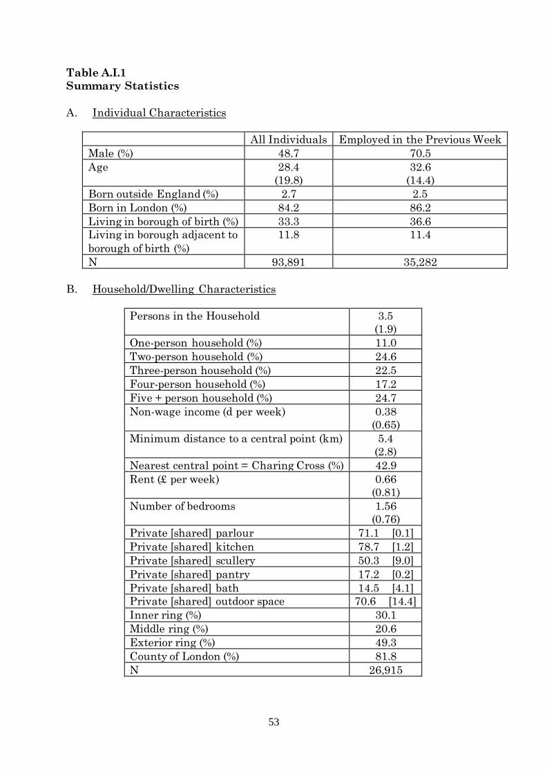
53
Table A.I.1
Summary Statistics
A. Individual Characteristics
All Individuals Employed in the Previous Week
Male (%) 48.7 70.5
Age 28.4
(19.8)
32.6
(14.4)
Born outside England (%) 2.7 2.5
Born in London (%) 84.2 86.2
Living in borough of birth (%) 33.3 36.6
Living in borough adjacent to
borough of birth (%)
11.8 11.4
N 93,891 35,282
B. Household/Dwelling Characteristics
Persons in the Household 3.5
(1.9)
One-person household (%) 11.0
Two-person household (%) 24.6
Three-person household (%) 22.5
Four-person household (%) 17.2
Five + person household (%) 24.7
Non-wage income (d per week) 0.38
(0.65)
Minimum distance to a central point (km) 5.4
(2.8)
Nearest central point = Charing Cross (%) 42.9
Rent (£ per week) 0.66
(0.81)
Number of bedrooms 1.56
(0.76)
Private [shared] parlour 71.1 [0.1]
Private [shared] kitchen 78.7 [1.2]
Private [shared] scullery 50.3 [9.0]
Private [shared] pantry 17.2 [0.2]
Private [shared] bath 14.5 [4.1]
Private [shared] outdoor space 70.6 [14.4]
Inner ring (%) 30.1
Middle ring (%) 20.6
Exterior ring (%) 49.3
County of London (%) 81.8
N 26,915

54
Table A.I.1
Summary Statistics, Continued
C. Employment Characteristics
Hours working in previous week 46.1
(8.3)
% age 16-65 reporting hours in previous week >0 54.9
Worked at least 40 hours (%) 90.8
Worked at least 48 hours (%) 57.1
Hours worked in a full-time week 46.9
(7.2)
% age 16-65 reporting hours in a full time week >0 56.1
Earnings in previous week (£) 2.34
(1.17)
Earnings in a full-time week (£) 2.38
(1.17)
Occupation = metal worker (%) 8.0
Occupation = electrical (%) 2.4
Occupation = makers of textile goods (%) 8.5
Occupation = food, drinks & tobacco (%) 3.1
Occupation = wood & furniture (%) 4.9
Occupation = printers & photographers (%) 2.5
Occupation = building trades (%) 4.4
Occupation = painters & decorators (%) 2.8
Occupation = transport and communications (%) 17.7
Occupation = Commerce, finance, insurance (%) 8.6
Occupation = personal service (%) 11.4
Occupation = clerk (%) 5.5
Occupation = warehousemen, storekeepers (%) 4.7
Occupation = other or unknown (%) 15.5
Armstrong skill category = professional (%) 0.1
Armstrong skill category = middling (%) 0.7
Armstrong skill category = skilled (%) 49.0
Armstrong skill category = semi-skilled (%) 24.0
Armstrong skill category = unskilled (%) 26.1
N 35,353
Notes: Standard errors are reported in parentheses for continuous variables. Age is reported as
zero in 9.2 percent of observations. We have excluded these observations from our calculations in
Table A.I.1 and included a dummy variable for the regressions reported in Tables 4 and 5.
Outside space comprises garden, yard, and allotment. Some households had multiple types of
outdoor space and some had both private and shared space.
Sources: Johnson, et. al. (1999) and authors’ calculations.

55
Appendix II: Coding GIS Coordinates and Distances
This appendix outlines our approach to GIS coding of home street addresses,
workplace locations, and the public transport network. We also outline how we use
these GIS coordinates to construct our measures of distance commuted, access to
public transport, and centrality. Finally, we examine measurement error and
biases that are likely to result from our approach and the likely implications for
our results.
I. Residential Addresses
Our approach to GIS coding home addresses is as follows. First, we have entered
the street name into streetmap.co.uk. If there exists exactly one modern street
with the same name that is located within the historic Metropolitan Borough listed
on the original record we assume this to be the residential address. We then take
the GIS coordinates from streetmap.co.uk. Occasionally there are multiple streets
of the same name within the same historic borough, e.g. two towns have a “High
St.”. Normally in these cases, the records themselves indicate the correct street.
For example, the streets may be listed as “High St., Woolwich” or “High St.,
Plumstead”. In cases such as this, the street is clearly identified even though the
official name of both streets is just “High St.” and both Woolwich and Plumstead
were in the Metropolitan Borough of Woolwich. In the small handful of cases
where there remained ambiguity, we have looked at additional information from
the record cards to determine the most likely correct address (e.g. whether
household members were working in Plumstead or Woolwich).
For about a quarter of the observations, we were unable to find the address listed
on the record card in streetmap.co.uk due to changes of street names. London was
extensively bombed during the Second World War. Many homes and even entire
neighbourhoods were damaged beyond repair (Ward 2015). After the War,
London’s urban planners “cleared” many War-damaged areas and other urban
slums. The clearances disproportionately affected working-class areas, as
wealthier areas which suffered minor bomb damage were quickly rebuilt. The
clearances often changed the physical layout of the area, for example replacing
low-rise dwellings with high-rise council housing (Sturm and Redding 2016).
To locate no-longer-extent streets, we began by searching the online indexed maps
from the LLPL (London School of Economics 2020). Because of the similarity of
coverage between the two surveys, most residential streets within the County of
London appearing in the NSLLL previously appeared in the LLPL. We were thus
normally able to find residential streets on the LLPL map and obtain GIS
coordinates from Ordinance Survey maps (National Library of Scotland 2020). In
cases where a street was not included in the LLPL index (particularly in the outer
boroughs not surveyed in the LLPL), we have searched other on-line resources
such as Medical Officer of Health Reports, Census Street Index, and various
genealogical web sites (Welcome Library 2021; Family Search 2021). Often, we
were able to find an exact or at least an approximate location for a residential
street, usually based on known locations for nearby streets that were listed in the

56
same source. Once we found the location, we then found the GIS coordinates using
Ordinance Survey maps (National Library of Scotland 2020).40
When entering GIS coordinates, we have used a single centroid for each home
address in the data.41 The centroid will either be the location used by
Streetmap.co.uk (for still-extent streets) or at approximately the middle of the
street (for no-longer-extent streets). The approach of using a single centroid
facilitates checking for inconsistencies in the data. It also makes it possible to
replicate our GIS coding procedure, as it avoids non-replicable ad hoc assumptions
about individual locations.
We believe that home addresses were very accurately recorded by the NSLLL
enumerators. The enumerators were instructed to visit each individual household;
hence they actually set foot on the residential street. We have been able to locate
well over 99 percent of home addresses in the data. Although our use of a single
centroid for each address will inevitably create some measurement error, we
believe that this measurement error is likely to be small because working-class
residential streets tended to be fairly short.
II Workplace addresses
Our approach to obtaining GIS coordinates for workplaces closely follows that of
home addresses. We searched streetmap.co.uk, followed by the indexed LLPL
maps, followed by other on-line sources to identify workplace streets or place
names. If this failed to produce a likely match, we searched old Ordinance Survey
maps (National Library of Scotland 2020) for similarly named streets nearby the
place of residence.42
There are several sources of measurement error for workplaces that are not
present for residences. First, the survey question for workplace is less precise than
residence, asking for “place of work” rather than “address”. Accordingly, the
responses were more varied than for home addresses, ranging from an exact
address, to just a street name, to a broader place name. About half the responses
are place names. Even place names can be imprecise. For example, “Greenwich”
is the name of both a Metropolitan Borough and the main town within the borough.
Where a place name is reported, we enter a common GIS coordinate using the
centroid of the smallest plausible geographic unit (e.g. town, rather than borough).
If the record card provides a general, but very broad area (e.g. “London” or “East
40 National Library of Scotland (2020) contains a variety of scalable modern and historic street
maps which can be uploaded side-by-side. Our GIS coding has primarily relied on OpenStreetMap;
Ordinance Survey (OS), 25 inches, 1892-1914; and OS 1/2500, 1944-1967. 41 We have used the street/borough pair when assigning centroids. Most streets were entirely
contained within a single borough and we assign a single set of GIS coordinates to these streets.
In cases were a street passed through multiple boroughs, we assign a single centroid for each
borough covered by the street. Street names tended to change at borough boundaries, so there are
very few residential streets with multiple coordinates in the data. 42 Since enumerators relied on residents to provide workplace addresses, there were fairly frequent
transcription errors or spelling mistakes on the original records. We were often able to find very
similar (or identically pronounced) workplace street names by searching the map around the home
address.

57
End”), we treated for place of work as missing unless we could identify a more
specific location based on the employer. The lack of precision in workplace
locations implies that our GIS coordinates are inherently subject to more
measurement error than for home addresses. In addition, commercial streets
tended to be longer than residential streets and thus there is likely to be more
measurement error for workplaces than residences, even in cases where a street
is listed for both. A final issue is that in about eight percent of observations with
pay reported the place of work is listed as “various” or “casual”. We assume these
workers to either be footloose (such as in the building trades) or itinerant. We do
not assign workplace locations to these workers.
A second difficulty identifying workplaces is that, unlike the home addresses, the
original record cards do not contain boroughs for workplace.43 This makes it more
difficult to identify the workplace location for common London street names,
unless the location is given on the original record card, e.g. “High St., Plumstead”.
In cases where a workplace address was ambiguous, we used other data from the
record such as home address, name of employer, and travel costs to identify the
most plausible location.44
A final issue results from the fact that enumerators never visited places of work,
instead they relied on information supplied by interviewees. At best, this meant
that the address was from second-hand information from the worker, rather than
directly from the enumerator. However, it is likely that the information was often
supplied by another member of the household. Although the New Survey
enumerators were explicitly instructed to make repeated visits to households in
order to get employment information from the income earner themselves, it is
known that Arthur Bowley, the overseer of the NSLLL, was willing to “sacrifice
accuracy to speed and simplicity” (Abernathy 2017; Hennock 1991).45 Responses
from someone other than individual workers themselves were probably widely
tolerated.46
43 The Johnson, et. al (1999) data contains a variable for workplace borough. However, this has
been constructed by the researchers and is not from the original record cards. We have created a
new variable for workplace borough by mapping the NSLLL area into approximately 500 square
meter grids. We map each observation into a cell using the GIS coordinates. We then map the grid
cells into boroughs. In cases where a grid cell is divided between more than one borough, we
mapped workplace addresses within the cell into boroughs by hand using Ordinance Survey maps
(OS 25 inches, 1892-1914). 44 Locations of larger employers often turned up in on-line searches, and we were often able to
identify precise GIS coordinates using this information. 45 It was noted in the original instructions to enumerators that “Vague estimates of husband’s
earnings by wife, of child’s by parent, or of lodger’s by landlady, should no t be entered until an
effort has been made to see the wage earner concerned” (New Survey, instructions issued to
investigators, quoted in Abernathy 2017). 46 Missing or imprecise workplace information is much more common in the NSLLL data for lodgers
than family members. It is difficult to reconcile this with earners supplying their own information,
but consistent with a single (non-working) resident supplying information for all household
members. In addition, the original record cards often provide relationships within households vis-
à-vis someone other than the likely head of household. Johnson, et. al (1999) have reclassified
household relationships using the age, gender, and earnings data to identify the head. The fact
that the head of household was frequently not correctly identified by the enumerators is strongly

58
Although the issues raised above imply that workplace addresses are more prone
to measurement error than home addresses, we believe that they are nevertheless
fairly accurate. We were able to obtain GIS coordinates for about 98 percent of
observations where a street or place name is given for place of work. When we
were unable to obtain workplace GIS coordinates, it was typically because either
the worker was itinerant or the original respondent did not supply the necessary
information. In about 12 percent of observations reporting earnings in the
previous week the information is either missing or unusable (“X”, “refused”,
“London”, etc.).
III Public transport
We have compiled a list of railway and London Underground stations in 1929
using historic Underground maps (Graham-Smith 2018), historic Ordinance
Survey maps (National Library of Scotland 2020), and Wikipedia lists of current
and historic stations (Wikipedia 2020a, 2020b, 2020c, 2020d). Wikipedia usually
provides GIS coordinates for rail and Underground stations and we cross-checked
these using historical Ordinance Survey maps (National Library of Scotland 2020).
We thus believe that these GIS coordinates are very accurate.
We obtained detailed information on bus and tram routes from London Historical
Research Group (2014) and Public (2020), respectively. However, neither source
indicates where vehicles stopped along the route. We have used OpenStreetMap
to find the location of modern bus stops and assumed that these correspond to
stops on the historic routes. Where the historic routes do not coincide with modern
routes, we have assumed that stops were 300-500 meters apart in central areas
and slightly further apart in outer areas, as with modern routes. We start with a
known stop on route, such as the route terminus or a railway station, and assign
stops approximately equidistant from this point. In addition to official stops, it was
generally possible for able-bodied passengers to board or leave a bus or tram at
any point where the vehicle was stopped and thus we also classify major
intersections as stops.47 There will be some measurement error in this approach
that is absent in our calculations for rail and Underground (for which we know the
exact location for each station), but this is likely to be fairly small, as tram and
bus stops were generally fairly close together.
IV Calculating Distances
We have used the GIS coordinates to calculate crow-flies distances between home,
work, the city centres, and public transport for each employed individual in the
sample. Conceptually, these distances are 1) the distance commuted (home to
work), 2) the centrality of their home or workplace (minimum distance to Charing
Cross or the Bank of England), and 3) access to public transport (distance to bus,
tram, Underground, or train). Figure A.II.1 shows these distances for one
individual. On the map, the residence is denoted H, the workplace is denoted W,
the nearest Underground stop to home is denoted U, and Charing Cross is denoted
suggestive that they made a single visit to the household and collected all information from the
person who answered the door. 47 The buses and trams of the 1930s were “routemaster” design with an open entrance at the
back. Passengers could embark or disembark at any point on route when the bus was stopped.

59
CX. The black line shows the crow-flies distance between home and work
(commuting distance). The green line shows the distance between home and
Charing Cross (centrality). The solid red line between H and U shows the distance
from home to the nearest underground station. The dotted and solid red lines
connected to this show the most plausible transport route to work (by underground
for two stops and a short walk to the workplace at the end). For ease of exposition,
we have not shown the other distances on this map.
To calculate distances, we use the great circle distance formula:
d = R*acos(sin(lat_a)*sin(lat_b) + cos(lat_a)*cos(lat_b)*cos(d_lon));
where: R = radius of the earth (6365 kilometres)
lat_a, lat_b = latitudes of points a and b
d_lon = difference in longitude between the two points.
There were a few exceptions to these principles in our calculations of distance. As
mentioned above, if a worker was deemed to be itinerant, we did not fix workplace
coordinates, and thus could not calculate distances. In addition, if the original
record card listed workplace as some variant of “local” or “nearby”, we assume a
commuting distance of 0.5 kilometres and that workplace centrality is the same
as home centrality. These cases account for approximately 2.4 percent of
observations.
There are also observations for which the distances between home and workplace
were very large. It is likely that these workers were stationed remotely and did
not commute on a daily basis. Thus, in our main analysis, we exclude the 76
observations where the distance between home and work was over 50 kilometres.
We have also set the cut-off at 20 kilometres (which excludes an additional 117
observations) and included long commutes in the analysis as robustness checks.
Our results are not particularly sensitive to the rule used for exclusion of outliers.
V. Measurement error and bias
For the most part, errors in our distance variables will simply be classical
measurement error, resulting from our inability to identify precise locations for
home, workplace, bus stops, and tram stops. As noted above, the extent of this
measurement error is likely to be larger for workplaces than for residences or
public transport. The consequence of this measurement error will be attenuation
bias in our estimates of the effects of distances on earnings. In other words, our
estimated returns to commuting in Section VII are likely to be biased downwards.
In addition to this measurement error, there exist two likely sources of systematic
bias in our variable for distance commuted. First, we are less likely to find
workplace locations for individuals who had longer commutes. When we could not
find a workplace through other means, our final approach was to search the map
in proximity to the worker’s residence. This approach helped locate numerous
workplaces, but it also implies that we are more likely to be missing data for

60
workplace location if a worker’s residence was further from home, and thus had a
longer commute. This will bias the estimated travel distances in Section VI
downwards. It will also bias the estimated effects of commuting on earnings
upwards. However, we do not feel that these biases are likely to be large because
we have been able to locate all but about two percent of workplaces named on the
original record cards.
A more serious concern results from our use of a single centroid for each residential
street and workplace location. As noted above, the use of a single centroid is likely
to result only in measurement error for residential addresses or workplace
locations, taken individually. However, the location of an individual’s workplace
is not independent of their residence. For example, a worker who resides on a short
north-south street that intersects a lengthy east-west workplace street near its
eastern end is more likely to work around the corner at the eastern end of the
workplace street than a couple kilometres away at the centroid of the street.
Similarly, a worker whose workplace is reported as a borough adjacent to their
borough of residence is more likely to be employed near the border of the two
boroughs than at the centroid of the workplace borough. Consequently, we are
likely to systematically overestimate the distance commuted, and thus
underestimate the returns to commuting.
The net bias resulting from our approach is almost certainly to underestimate the
returns to distance commuted. On the other hand, there is likely to be little bias
in our estimated returns to access to public transport, as these distances are
measured with little error. As a result, we think our results in Section VII
represent a lower bound on the returns to distance commuted but are fairly
accurate on the returns to access to public transport.
References
Abernethy, Simon T. (2017). “Deceptive data? The role of the investigators in the
New Survey of London Life and Labour 1928–32.” Historical Methods A
Journal of Quantitative and Interdisciplinary History, 50(1):1-15.
Family Search (2021). Census Street Index.
https://www.familysearch.org/wiki/en/Census_Street_Indexes [Accessed
25/9/2020].
Graham-Smith, Darien (2018). “The history of the tube map”. Londonist.
https://londonist.com/2016/05/the-history-of-the-tube-map [Accessed
25/9/2020].
Hennock, E. P. (1991). “Concepts of poverty in the British social surveys from
Charles Booth to Arthur Bowley.” In M. Bulmer, K. Bales, and K. K. Sklar,
eds. The Social Survey in Historical Perspective. (Cambridge: Cambridge
University Press), pp. 189-217.
Johnson, Paul A., Bailey, Roy E., Baines, Dudley E., Raspin, Anna, Hatton,
Timothy J. (1999). New Survey of London Life and Labour, 1929-1931. [data
collection]. 2nd Edition. UK Data Service. SN: 3758,
http://doi.org/10.5255/UKDA-SN-3758-1.

61
https://beta.ukdataservice.ac.uk/datacatalogue/studies/study?id=3758
[Accessed 25/9/2020].
London Historical Research Group, The Omnibus Society (2014): Motor Omnibus
Routes in London, vol. 10A (1st January 1931 to 31st December 1932)
(Sevenoaks: London Historical Research Group).
London School of Economics (2020). Charles Booth’s London: Poverty Maps and
Police Notebooks. https://booth.lse.ac.uk/map/14/-0.1174/51.5064/100/0
[accessed 13/9/2020].
National Library of Scotland (2020). Side-by-Side Map Images.
https://maps.nls.uk/ [Accessed 25/9/2020].
Public (2020). “Trams in London.”
http://sharemap.org/public/Trams_in_London#!webgl [Accessed 25/9/2020].
Redding, Stephen and Sturm, Daniel (2016). “Estimating neighbourhood effects:
evidence from War-time destruction in London.” Mimeo, London School of
Economics.
Streetmap (2020). https://www.streetmap.co.uk/ [accessed 25/9/2020].
Ward, Laurence (2018). The London County Council Bomb Damage Maps, 1939-
1945. (London: Thames & Hudson).
Welcome Library (2021). The Medical Officer of Health Reports.
https://wellcomelibrary.org/moh/about-the-reports/about-the-medical-
officer-of-health-reports/ [accessed 25/9/2020].
Wikipedia (2020a). “List of London railway stations.”
https://en.wikipedia.org/wiki/List_of_London_railway_stations [accessed
25/9/2020].
Wikipedia (2020b). “List of closed railway stations in London.”
https://en.wikipedia.org/wiki/List_of_closed_railway_stations_in_London
[accessed 25/9/2020].
Wikipedia (2020c). “List of London Underground stations.”
https://en.wikipedia.org/wiki/List_of_London_Underground_stations
[accessed 25/9/2020].
Wikipedia (2020d). “List of former and unopened London Underground stations.”
https://en.wikipedia.org/wiki/List_of_former_and_unopened_London_Under
ground_stations [accessed 25/9/2020].

62
Figure A.II.1
Distances for One Individual

63
Appendix III: Costs and Benefits of Commuting and Calculating Poverty
Lines
I. Costs and benefits of Commuting
Table 6 shows the costs and benefits of commuting. The calculations in this table
are very much back-of-the-envelope, but are informed by stylized facts from
Ponsonby and Ruck (1930) and from the New Survey data. In this appendix we
describe the assumptions behind these calculations and examine their historical
basis.
Crow-flies distances:
The distances in the first column are arbitrary round numbers, which cover the
range of distances commuted. The range of distances covers virtually all workers
who were not working “on the spot” (the term used by Ponsonby and Ruck (1930)
to describe the proximity of employment to residence in the 1890s). Approximately
86 percent of income earners in the sample travelled at least 500 meters;
approximately 99 percent travelled at most 16 kilometres.
Transport mode:
Ponsonby and Ruck (1930) state that workers typically walked up to 1.6
kilometres, buses and trams were used interchangeably for distances of 1.6 to 3.2
kilometres, the Underground was typically used for distances of 3.2 to 19.3
kilometres, and trains were used for longer distances or as a replacement for the
Underground in places where it was not available. Approximately 82.9 percent of
workers with non-missing transport costs who travelled distances of up to 1.6
kilometres, reported costs of exactly zero, and thus must have walked or cycled.
Approximately, 83.7 percent of individuals with non-missing transport costs who
commuted over 1.61 kilometres, reported positive costs, and thus must have used
public transport. We do not observe the mode of transport, but the relationship
between proximity to stops/stations and commuting distances shown in the
regressions in Table 4 is consistent with the pattern reported by Ponsonby and
Ruck (1930).
Distance walked:
We construct as the crow-flies, distances i.e. in a straight line. The urban layout
rarely allows this to be the actual route, thus actual distance travelled must be
greater than crow-flies distance. There exists a substantial literature in geography
on the difference between crow-flies and actual distances (Rietveld, et. al. 1999
and Underhill 2020). We assume, somewhat arbitrarily, that walking-only
journeys were 25 percent longer than the crow-flies distance. Any journey
involving public transport would have also involved walking from home to
transport and from transport to work. Table 3 shows the average distance from
home and work to each public transport mode. However, workers would have
chosen their mode of transport at least partly based on proximity, so the walking

64
distance to the chosen mode of transport will have on average been less than for
modes not used. We assume 300 meters of total walking at both ends for a one-
way bus journey, about 75 percent of the sum of average distances from the nearest
bus stop to home and workplace. We also assume 300 meters of walking for a one-
way tram journey. This is considerably less than the average distance shown in
Table 3; however, one would expect that the distance walked by tram users would
have been approximately the same as bus users, as the two modes of transport
were used interchangeably. We assume 600 meters of walking at both ends for a
one-way Underground or train journey, about 75 percent of the maximum distance
that geographers have argued that commuters are willing to walk to these modes
of transport (Daniels and Mulley 2013).
Distance on public transport:
As with walking, public transport generally does not travel in a straight line and
this adds to the total distance. On the other hand, in many cases workers can
choose between stops which are approximately equidistant to home (work). If there
are two approximately equidistant stops from home, a worker would have been
more likely to use the one closer to their work in order to minimize total travel
time. This will at least partly offset the effect of added distance due to non-linear
transport routes, and thus we assume that the travel distance for public transport
is only 10 percent more than the crow-flies distance of total travel.
With each of our assumptions about distance, there is likely to be considerable
heterogeneity across individuals and locations. The assumptions are not verifiable
in the data, so it is also possible that there is some error on average. However, it
is unlikely that modest errors in either direction will have a substantial impact on
our conclusions in Section VI.
Walking and public transport time:
Time is calculated as distance (from columns 3 and 4 in Table 6) divided by speed.
Following Leunig (2006), we use 4 kilometres per hour as a typical urban walking
speed. We take public transport speeds from Table 2. Neither Ponsonby and Ruck
(1930) nor London Statistics provide train speeds after the first World War and
we assume that average speeds in 1930 were 10 percent faster than those reported
in London Statistics for 1907-08.
Implied return:
We use the first regression in Table 5, evaluated at the tenth, twenty fifth, and
fiftieth percentiles of the weekly earnings distribution (180d, 300d, and 583.5d) to
calculate the returns to commuting the distances shown in the first column.
Specifically, we estimate the returns as:
Exp[ln(WE) + .02577d - .00489d2] – Exp[ln(WE)]
where:

65
WE = weekly earnings (in pence), evaluated at the 10th, 25th, and 50th percentile d = distance commuted, in kilometres (from Table 6, column 1)
Monetary costs:
We use reported transport expenses from the New Survey data and the description
of travel costs from Ponsonby and Ruck (1930) to determine a “typical” cost for the
journey in each row. Public transport fares were set by zones, which were
imperfectly correlated to distance. For any given distance and mode of transport
there may have been multiple fares, depending on the embarkation and
disembarkation stations. The monetary costs reported in Table 6 are the range of
typical fares reported in the New Survey data for workers commuting distances
within 500 meters of the crow-flies distances in column 1.48
Implied time costs:
The total time spent commuting is the sum of walking time, transport time, and
waiting time. We assume five minutes waiting time for the bus and tram and eight
minutes for the train and Underground. We assume a longer time for train and
Underground because the platform was physically removed from the entrance to
the station. Following an extensive literature on the value of travel time saved, we
use 50 percent of salary as the implied cost of commuting time (Wardman 1998;
Zamparini and Reggiani 2007). In the second column of Table 6, we assume a
single mode of transport. In practice, some commuters, particularly those with
longer commutes, may have needed to transfer between modes and thus incurred
additional waiting time.
II. The Hatton-Bailey Poverty Line
The appendix in Hatton and Bailey (1998) outlines their approach to constructing
household poverty lines. To briefly summarize, they allocate minimum required
expenditures on food and clothing, rent, and fuel. The minimum required
expenditure on food and clothing is based on age and sex of the individual and
ranges from 36d per week for a child under age 1 to 102d per week for males aged
18 and over. The minimum required rental expenditure is based on a standard of
no more than two individuals to a room and a cost of 60d per week for one room,
102d per week for two rooms, 126d per week for three rooms, and 30d per week for
each additional room. The minimum required expenditure on fuel is 36d per week,
plus an additional 2d in South London. A household is classified as poor if the sum
of these minimum expenditures and actual household expenditures on transport
and National Insurance is greater than their total income from all sources. The
New Survey reports income in previous week and in a full-time week and Hatton
and Bailey (1998) use income from the previous week for the poverty calculations.
The estimated poverty lines using this approach are 198, 292, 392, 588 pence per
week for a household with only a single adult male, a married couple, a couple
with one child, and a couple with three children, respectively. Hatton and Bailey
48 The New Survey data typically reports weekly expenditures on transport. We divide this by 12
to find one-way fares. In each case, the range reported in Table 6 covers both the median and
modal fare.

66
(1998) estimate that 12.11 percent of households and 12.0 percent of individuals
fell below the poverty line.
We have made two adjustments to their calculations. First, approximately 9.2
percent of individuals in the New Survey have a reported age of exactly zero. This
is an implausibly large number and almost certainly indicates that age was not
reported in most of these observations. We have reclassified these individuals as
adults and adjusted required expenditure on food and clothing if 1) they had an
occupation or reported earnings or hours worked or 2) their relationship to the
head of household indicates they must have been an adult (e.g. wife or
grandfather). If the individual was not an income earner and was plausibly a child
(e.g. son or nephew of the head), we use a value of zero for age and assign minimum
expenditure accordingly. The reclassification of children age zero to adults (age
18+) increases the minimum expenditure on food and clothing from 38d per week
to 102d per week for 3742 men and to 94d per week for 4792 women. It is likely
that many of those we still classify as age zero were actually older and thus would
require greater expenditures than for an infant, so our upwards adjustment to the
poverty line is a lower-bound. Secondly, both National Insurance contributions
and transport expenses are frequently missing in the New Survey data. Among
individuals reporting earnings or hours in the previous week, approximately 30
percent are missing data for transport costs and approximately 20 percent are
missing data for National Insurance contributions. We have handled missing data
in two ways: constructing a lower-bound poverty line where missing observations
are replaced by a value of zero and an expected value poverty line where missing
observations are replaced by the overall sample mean. These reclassifications
increase the poverty line for 4730 households and increase the number of
individuals classified as poor from 12.0 percent of the sample (Hatton and Bailey
1998, p. 584) to 16.7 percent of the sample (lower-bound poverty line) or 20.6
percent of the sample (expected value poverty line).
References
Daniels, Rhonda and Mulley, Corinne (2013). “Explaining walking distance to
public transport: The dominance of public transport supply.” Journal of
Transport and Land Use,
6(2): 5-20.
Leunig, Tim (2006). “Time is money: a re-assessment of the passenger social
savings from Victorian British railways.” Journal of Economic History,
66(3): 635-73.
London County Council (various years). London Statistics. (London: P. S. King
and Son).
Ponsonby, G. and Ruck, S. K. (1930). “Travel and mobility”. In Llewellyn-Smith,
Hubert, eds. The New Survey of London Life and Labour. (London: P. S.
King), pp. 171-99.
Rietveld, Piet, Zwart, Bert, van Wee, Bert, van den Hoorn, Toon (1999). “On the
relationship between travel time and travel distance of commuters.” Annals
of Regional Science, 33(3): 269-87.

67
Underhill, Keziah (2020). “December visualisation blog: crow flies vs. OD paths.”
https://www.basemap.co.uk/december-visualisation-blog-crow-flies-vs-od-
paths/ [accessed 23/02/2021].
Wardman, Mark (1998). “The value of travel time: A review of British evidence.”
Journal of Transport Economics and Policy, 32(3): 285-316.
Zamparini, Luca and Reggiani, Aura (2007). “Meta-analysis and the value of travel
time savings: a transatlantic perspective in passenger transport.” Networks
and Spatial Economics, 7(4): 377-96.

68
Appendix IV: Additional Tables and Figures
Table A.IV.1: Estimated Effects of Control Variables on Labour Force
Participation
(1) (2) (3) (4) (5) (6) (7)
Hours>0 In Work Distance Distance
(Heckman)
Transport
Costs=0
Distance
<1 Km
Distance
>3.2 Km
Age -1.558*
(0.056)
-1.630*
(0.053)
10.195*
(1.478)
6.873*
(1.771)
-1.130*
(0.001)
-0.633*
(0.122)
1.104*
(0.127)
Age squared 0.009*
(0.001)
0.009*
(0.001)
-0.144*
(0.020)
-0.129*
(0.020)
0.170*
(0.020)
0.011*
(0.002)
-0.016*
(0.002)
Age reported as
zero
-0.599*
(0.012)
-0.570*
(0.011)
1.825*
(0.276)
0.518
(0.484)
-0.131*
(0.028)
-0.064*
(0.024)
0.186*
(0.024)
Female -0.341*
(0.003)
-0.380*
(0.003)
-0.418*
(0.062)
-1.041*
(0.200)
-0.015*
(0.007)
0.027*
(0.006)
-0.046*
(0.006)
Born in England 0.077*
(0.007)
0.070*
(0.007)
-0.176
(0.185)
-0.004
(0.152)
0.019
(0.014)
-0.001
(0.012)
-0.022
(0.012)
Born in London 0.188*
(0.006)
0.192*
(0.006)
-0.214
(0.139)
0.163
(0.159)
-0.009
(0.011)
0.001
(0.009)
-0.014
(0.009)
Born and lives in
the same borough
-0.029*
(0.005)
-0.037*
(0.004)
-0.165*
(0.081)
-0.187*
(0.090)
0.031*
(0.009)
0.010
(0.007)
-0.023*
(0.008)
Borough is
adjacent to birth
borough
-0.055*
(0.006)
-0.071*
(0.006)
-0.209*
(0.102)
-0.280*
(0.138)
-0.004
(0.013)
-0.019
(0.011)
0.009
(0.012)
Other family pay -0.000*
(0.000)
-0.001*
(0.000)
Non-labour income
household
-0.002*
(0.000)
-0.002*
(0.000)
Observations 51,970 51,970 23,254 51,970 19,147 23,254 23,254
Notes: Coefficients on Age and Age squared are multiplied by 100. See Table 4 for additional
results and notes.
Sources: Johnson, et. al. (1999) and authors’ calculations.

69
Table A.IV.2: Distance Effects on Labour Force Participation: All Family Members in a Household
(1) (2) (3) (4) (5) (6) (7)
Hours>0:
Probit
In
Work:
Probit
Dist. to
Work:
OLS
Dist. to
Work:
Heckman
Trans.
Costs=0:
Probit
Dist. to
Work<1Km:
Probit
Dist. to
Work>3.2Km:
Probit
Distance-Centre -0.001
(0.002)
-0.005*
(0.002)
0.441*
(0.035)
0.410*
(0.038)
-0.052*
(0.003)
-0.057*
(0.003)
0.060*
(0.003)
Distance Home-Train 0.024*
(0.005)
0.007
(0.005)
-0.100
(0.105)
-0.072
(0.109)
0.011
(0.009)
-0.010
(0.008)
-0.008
(0.008)
Distance Home-
Underground
0.005
(0.003)
-0.003
(0.003)
-0.182*
(0.080)
-0.179*
(0.067)
0.039*
(0.006)
0.041*
(0.005)
-0.026*
(0.005)
Distance Home-Tram -0.007
(0.006)
-0.003
(0.006)
-0.063
(0.129)
-0.102
(0.133)
-0.007
(0.012)
-0.040*
(0.010)
0.001
(0.010)
Distance Home-Bus -0.004
(0.010)
-0.026*
(0.009)
-0.064
(0.189)
-0.060
(0.220)
-0.009
(0.019)
-0.043*
(0.016)
0.006
(0.016)
Observations 67,584 67,584 34,342 67,584 28,880 34,294 34,294
R-squared 0.278 0.351 0.029 0.047 0.042 0.063
Sample mean 0.512 0.582 3.22 3.22 0.418 0.294 0.332
Notes: See notes in Table 4.
Sources: Johnson, et. al. (1999) and authors’ calculations.

70
Table A.IV.3 Estimated Effects of Control Variables on Earnings
(1) (2) (3) (4) (5) (6)
Related
to Head
Related to
Head: Heckman
Related to
Head: Age<25
Children
of Head: Age<25
All All: HH
Fixed Effects
Age 0.146* (0.003)
0.146* (0.003)
0.491* (0.015)
0.495* (0.015)
0.098* (0.001)
0.110* (0.001)
Age2 -0.002* (0.000)
-0.002* (0.000)
-0.010* (0.000)
-0.010* (0.000)
-0.001* (0.000)
-0.001* (0.000)
Missing Age 2.586*
(0.039)
2.595*
(0.038)
6.131*
(0.140)
6.246*
(0.143)
2.054*
(0.022)
2.187*
(0.030)
Male 0.266*
(0.007)
0.266*
(0.007)
0.211*
(0.007)
0.202*
(0.007)
0.321*
(0.006)
0.272*
(0.008)
Born in
England
0.042*
(0.016)
0.043*
(0.016)
0.006
(0.018)
0.007
(0.019)
0.039*
(0.008)
0.058*
(0.014)
Born in
London
-0.001
(0.010)
-0.001
(0.010)
0.016
(0.009)
0.018*
(0.009)
0.003
(0.007)
-0.024
(0.014)
Born and lives
in the same borough
0.102*
(0.008)
0.102*
(0.008)
0.015
(0.008)
0.014
(0.008)
0.074*
(0.005)
0.161*
(0.010)
Lives in an adjacent
borough
0.019 (0.013)
0.019 (0.013)
0.004 (0.013)
0.013 (0.013)
0.024* (0.007)
0.082* (0.014)
Hours last
week
0.017*
(0.001)
0.016*
(0.001)
0.010*
(0.001)
0.009*
(0.001)
0.016*
(0.000)
0.018*
(0.000)
Hours missing 0.615*
(0.036)
0.615*
(0.036)
0.351*
(0.041)
0.305*
(0.041)
0.635*
(0.024)
0.672*
(0.028)
Quarrying 0.056
(0.132)
0.056
(0.132)
0.136
(0.127)
0.129
(0.134)
0.167*
(0.054)
0.132
(0.120)
Brick/Glass
worker
0.106
(0.099)
0.105
(0.099)
0.139
(0.087)
0.117
(0.089)
0.165*
(0.048)
0.198
(0.084)
Chemicals 0.178
(0.095)
0.179
(0.094)
0.184
(0.080)
0.178
(0.082)
0.170*
(0.042)
0.196
(0.078)
Metals 0.144
(0.093)
0.144
(0.093)
0.134
(0.078)
0.132
(0.080)
0.174*
(0.040)
0.165*
(0.073)
Electro-plate 0.090
(0.121)
0.090
(0.120)
0.107
(0.111)
0.079
(0.116)
0.240*
(0.062)
0.144
(0.099)
Electricians 0.115 (0.093)
0.115 (0.093)
0.103 (0.079)
0.095 (0.081)
0.185* (0.041)
0.124 (0.075)
Watchmakers 0.151 (0.115)
0.152 (0.114)
0.113 (0.090)
0.107 (0.092)
0.226* (0.055)
0.096 (0.098)
Leather 0.104 (0.095)
0.105 (0.094)
0.131 (0.079)
0.111 (0.081)
0.175* (0.043)
0.130 (0.077)
Textiles 0.036 (0.096)
0.035 (0.096)
0.047 (0.083)
0.038 (0.085)
0.092 (0.048)
0.102 (0.085)
Dressmakers 0.108 (0.093)
0.108 (0.092)
0.112 (0.078)
0.101 (0.080)
0.166* (0.040)
0.103 (0.073)
Food/Drink 0.131
(0.093)
0.132
(0.093)
0.148
(0.079)
0.142
(0.081)
0.169*
(0.040)
0.170
(0.074)
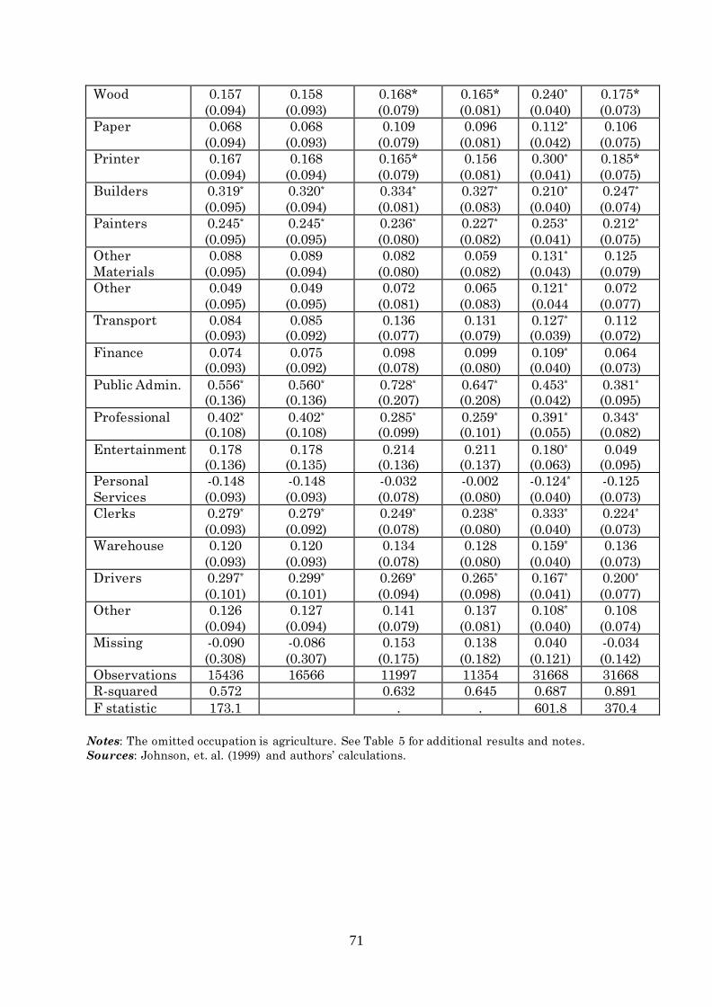
71
Wood 0.157
(0.094)
0.158
(0.093)
0.168*
(0.079)
0.165*
(0.081)
0.240*
(0.040)
0.175*
(0.073)
Paper 0.068
(0.094)
0.068
(0.093)
0.109
(0.079)
0.096
(0.081)
0.112*
(0.042)
0.106
(0.075)
Printer 0.167
(0.094)
0.168
(0.094)
0.165*
(0.079)
0.156
(0.081)
0.300*
(0.041)
0.185*
(0.075)
Builders 0.319*
(0.095)
0.320*
(0.094)
0.334*
(0.081)
0.327*
(0.083)
0.210*
(0.040)
0.247*
(0.074)
Painters 0.245*
(0.095)
0.245*
(0.095)
0.236*
(0.080)
0.227*
(0.082)
0.253*
(0.041)
0.212*
(0.075)
Other
Materials
0.088
(0.095)
0.089
(0.094)
0.082
(0.080)
0.059
(0.082)
0.131*
(0.043)
0.125
(0.079)
Other 0.049
(0.095)
0.049
(0.095)
0.072
(0.081)
0.065
(0.083)
0.121*
(0.044
0.072
(0.077)
Transport 0.084 (0.093)
0.085 (0.092)
0.136 (0.077)
0.131 (0.079)
0.127* (0.039)
0.112 (0.072)
Finance 0.074 (0.093)
0.075 (0.092)
0.098 (0.078)
0.099 (0.080)
0.109* (0.040)
0.064 (0.073)
Public Admin. 0.556* (0.136)
0.560* (0.136)
0.728* (0.207)
0.647* (0.208)
0.453* (0.042)
0.381* (0.095)
Professional 0.402* (0.108)
0.402* (0.108)
0.285* (0.099)
0.259* (0.101)
0.391* (0.055)
0.343* (0.082)
Entertainment 0.178 (0.136)
0.178 (0.135)
0.214 (0.136)
0.211 (0.137)
0.180* (0.063)
0.049 (0.095)
Personal
Services
-0.148
(0.093)
-0.148
(0.093)
-0.032
(0.078)
-0.002
(0.080)
-0.124*
(0.040)
-0.125
(0.073)
Clerks 0.279*
(0.093)
0.279*
(0.092)
0.249*
(0.078)
0.238*
(0.080)
0.333*
(0.040)
0.224*
(0.073)
Warehouse 0.120
(0.093)
0.120
(0.093)
0.134
(0.078)
0.128
(0.080)
0.159*
(0.040)
0.136
(0.073)
Drivers 0.297*
(0.101)
0.299*
(0.101)
0.269*
(0.094)
0.265*
(0.098)
0.167*
(0.041)
0.200*
(0.077)
Other 0.126
(0.094)
0.127
(0.094)
0.141
(0.079)
0.137
(0.081)
0.108*
(0.040)
0.108
(0.074)
Missing -0.090
(0.308)
-0.086
(0.307)
0.153
(0.175)
0.138
(0.182)
0.040
(0.121)
-0.034
(0.142)
Observations 15436 16566 11997 11354 31668 31668
R-squared 0.572 0.632 0.645 0.687 0.891
F statistic 173.1 . . 601.8 370.4
Notes: The omitted occupation is agriculture. See Table 5 for additional results and notes.
Sources: Johnson, et. al. (1999) and authors’ calculations.
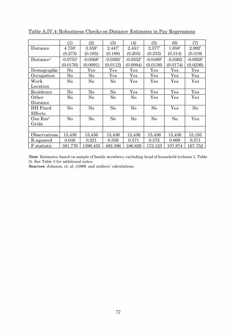
72
Table A.IV.4: Robustness Checks on Distance Estimates in Pay Regressions
(1) (2) (3) (4) (5) (6) (7)
Distance 4.738*
(0.273)
3.359*
(0.165)
2.447*
(0.188)
2.451*
(0.203)
2.577*
(0.233)
1.858*
(0.314)
2.992*
(0.319)
Distance2 -0.0755*
(0.0176)
-0.0568*
(0.0091)
-0.0392*
(0.0112)
-0.0352*
(0.0094)
-0.0489*
(0.0138)
-0.0262
(0.0174)
-0.0828*
(0.0236)
Demographic No Yes Yes Yes Yes Yes Yes
Occupation No No Yes Yes Yes Yes Yes
Work Location
No No No Yes Yes Yes Yes
Residence No No No Yes Yes Yes Yes
Other
Distance
No No No No Yes Yes Yes
HH Fixed
Effects
No No No No No Yes No
One Km2 Grids
No No No No No No Yes
Observations 15,436 15,436 15,436 15,436 15,436 15,436 15,185
R-squared 0.046 0.521 0.559 0.571 0.572 0.869 0.571
F statistic 381.776 1396.455 482.596 186.829 173.123 107.874 167.752
Note: Estimates based on sample of family members, excluding head of household (column 1, Table
5). See Table 5 for additional notes.
Sources: Johnson, et. al. (1999) and authors’ calculations.

73
Table A.IV.5: Further Robustness Checks on Distance Estimates in Pay Regressions
(1) (2) (3) (4) (5) (6) (7) (8)
Unlimited
Distance
Armstrong
Skill
Exclude
highest
earner
No
Bartlett
sample
Discrete
Distance:
Non-Head Family
Discrete
Distance:
All Family
Only
Heads
Discrete
Distance:
Only Heads
Distance-Work 2.337*
(0.177)
2.999*
(0.239)
3.040*
(0.267)
2.595*
(0.258)
1.272*
(0.167)
Distance2 -0.0304*
(0.0093)
-0.0600*
(0.0143)
-0.0734*
(0.0154)
-0.0506*
(0.0153)
-0.0418*
(0.0118)
Ref: Distance<0.5
Km
Distance: 0.5-1 0.038*
(0.013)
0.029*
(0.009)
0.025*
(0.010)
Distance: 1-2 0.046*
(0.012)
0.042*
(0.008)
0.041*
(0.009)
Distance: 2-3 0.070*
(0.013)
0.061*
(0.009)
0.047*
(0.010)
Distance: 3-4 0.081*
(0.014)
0.074*
(0.009)
0.062*
(0.011)
Distance: 4-5 0.132*
(0.016)
0.102*
(0.010)
0.057*
(0.012)
Distance: 5-10 0.166*
(0.015)
0.126*
(0.009)
0.071*
(0.010)
Distance: 10+ 0.236* (0.021)
0.183* (0.013)
0.117* (0.013)
Observations 15,441 15,436 15,436 13,298 15,436 31,195 15,758 15,758
R-squared 0.572 0.553 0.571 0.567 0.572 0.686 0.512 0.512
F statistic 172.912 199.754 173.805 147.639 166.068 574.471 68.871 67.419
Notes: See notes in Table 5.
Sources: Johnson, et. al. (1999) and authors’ calculations.

74
Figure A.IV.1. Commuting Destinations for Residents of All Boroughs


