
The Impact of Gradient Wind Imbalance on Tropical Cyclone Intensificationwithin Ooyama’s Three-Layer Model
THOMAS FRISIUS AND MARGUERITE LEE
Meteorological Institute, University of Hamburg, Hamburg, Germany
(Manuscript received 3 November 2015, in final form 8 June 2016)
ABSTRACT
This paper addresses the validity of the gradient wind balance approximation during the intensification
phase of a tropical cyclone in Ooyama’s three-layer model. For this purpose, the sensitivity to various model
modifications is examined, given by the inclusion of (i) unbalanced dynamics in the free atmosphere, (ii)
unbalanced dynamics in the slab boundary layer, (iii) a height-parameterized boundary layermodel, and (iv) a
rigid lid. The most rapid intensification occurs when the model employs the unbalanced slab boundary layer,
while the simulation with the balanced boundary layer reveals the slowest intensification. The simulation with
the realistic height-parameterized boundary layer model exhibits an intensification rate that lies in between.
Intensification is induced by a convective ring in all experiments, but a distinct contraction of the radius of
maximum gradient wind only takes place with unbalanced boundary layer dynamics. In all experiments the
rigid lid and the balance approximation for the free atmosphere have no crucial impact on intensification,
and a linear stability analysis cannot explain the found sensitivity to intensification. Most likely the nonlinear
momentum advection term plays an important role in the boundary layer. It is found on the basis of a di-
agnostic radial mass flux equation that the source term for latent heat provides the largest contribution to
intensification and contraction. Furthermore, it turns out that the position of the convective ring inside or
outside of the radius of maximum gradient wind (RMGW) is of vital importance for intensification and most
likely explains the large impact of boundary layer imbalance.
1. Introduction
The mechanism for tropical cyclone intensification is
still controversially debated [for a review, see Smith and
Montgomery (2015)], although many numerical non-
linear models can capture this phenomenon properly.
The numerical axisymmetric model developed by Ooyama
(1969, hereafter O69) was one of the first to reveal tropical
cyclone intensification. The model is based on the hy-
drostatic Boussinesq equations and has three layers of
uniform density, where the lowest one is a slab boundary
layer. This simple model conception enables a better
understanding of the intensification process and has the
advantage of a high numerical efficiency. However, the
Ooyama model includes the balance approximation—
that is, the tangential wind underlies the gradient wind
balance—and it is questionable if this assumption is
justified during the intensification stage, when the rate at
which pressure falls becomes large in magnitude. In the
present study we will analyze the impact of this assump-
tion by relaxing the balance assumption within Ooyama’s
model. Indeed, K.V. Ooyama (1968, unpublished manu-
script)1 presented results of a modified three-layer model
that includes an unbalanced boundary layer. He found
more realistic solutions than with the original model (see
also Smith and Montgomery 2008). An unbalanced non-
axisymmetric Ooyama model was also developed by
Schecter and Dunkerton (2009) and compared to a cloud-
resolving model by Schecter (2011). These studies in-
vestigated the sensitivity of tropical cyclone formation and
maximum intensity with respect to various model param-
eters but did not address the impact of gradient wind
imbalance.
Another aimof this study is to advance understanding of
the intensificationmechanism. The balance approximation
has the advantage that the cause of tangential wind rise can
be revealed by the Sawyer–Eliassen equation (Shapiro and
Corresponding author address: Thomas Frisius, CliSAP, Uni-
versität Hamburg, Grindelberg 5, D-20144 Hamburg, Germany.
E-mail: [email protected]
1 ‘‘Numerical Simulation of Tropical Cyclones with an Axi-
symmetric Model.’’
SEPTEMBER 2016 FR I S IU S AND LEE 3659
DOI: 10.1175/JAS-D-15-0336.1
� 2016 American Meteorological SocietyUnauthenticated | Downloaded 12/25/21 04:19 AM UTC

Willoughby 1982; Bui et al. 2009). This diagnostic equation
results from the time derivative of the thermal wind bal-
ance equation. In the Ooyama model a simpler diagnostic
equation can be derived because of the three-layer formu-
lation. We will see that time differentiation of the gradient
wind balance equation yields a single ordinary differential
equation for the radial mass flux when a rigid lid is
assumed. Shapiro and Willoughby (1982) also analyzed
tropical cyclone intensification, and they found that a
single point source for heat can induce contraction of the
wind maximum and intensification. We will see that this
convective ring contraction scenario also does take place
in the Ooyama model and that the findings by Shapiro
and Willoughby (1982) are indeed relevant. However,
less clear is the role of the boundary layer. The boundary
layer supplies the necessary latent energy that is released
in the contracting convective ring. Smith andMontgomery
(2008) found that the gradient wind imbalance has a large
impact on the wind profiles in a steady-state slab boundary
layer model of a tropical cyclone. It is likely that this also
has an effect on the strength and position of the convec-
tive ring fed by boundary layer air. Therefore, the balance
assumption in the boundary layer could sensitively influ-
ence the intensification rate. On the other hand, Kepert
(2010a,b) and Williams (2015) found by comparing the
slab boundary layer model with a height-resolving bound-
ary layer model that the former tends to overestimate su-
pergradient winds and vertical velocities. Kepert (2010b)
suggested using a height-parameterized boundary layer
model instead, which can be coupled to theOoyamamodel
indeed, as we will demonstrate in this paper.
The paper is organized as follows. Section 2 contains
the model description and the outline of the simulations.
In section 3, results of the performed simulations are
presented and the differences due to the balance ap-
proximation are identified. Section 4 clarifies the in-
tensification mechanism by analyzing the linearized
equations and evaluating the diagnostic equation for the
induced secondary circulation. Finally, the conclusions
are summarized in section 5.
2. Description of the model
Ooyama’s model includes three layers lying upon each
other, which is sketched in Fig. 1. The interface between
the middle and the upper layers is a free material surface,
while the interface between the lower andmiddle layers is
fixed but permeable. The lowermost layer forms the
boundary layer where microturbulent exchange with the
ocean surface is relevant. Convection can pervade all in-
terfaces, and it gives rise to the vertical mass fluxes Qb,1,
Qb,2, and Q1;2. The density of the two lower layers is r0,
while that of the upper layer takes the value �r0 with �, 1.
In the following subsections the governing equations, the
physical parameterization schemes, the rigid-lid modifi-
cation, Kepert’s height-parameterized boundary layer
model, and the performed experiments are outlined.
a. Governing equations of the free-surface Ooyamamodel
The governing equations of the free-surface Ooyama
model are as follows:
d1
�›u
j
›t1 u
j
›uj
›r
�2
�f 1
yj
r
�yj
52›P
j
›r1 d
1(D
y,uj1D
h,uj), j5 1; 2, (1)
›yj
›t1 z
juj5D
y,yj1D
h,yj, j5 1; 2, (2)
d2
�d3
›ub
›t1u
b
›ub
›r
�2
�f 1
yb
r
�yb
52›P
1
›r1 d
2(D
y,ub1D
h,ub1D
s,ub), (3)
d2d3
›yb
›t1 z
bub5 d
2(D
y,yb1D
h,yb)1D
s,yb, (4)
›ue,b
›t1 u
b
›ue,b
›r5 (D
y,ue,b1D
h,ue,b1D
s,ue,b), (5)
›h1
›t11
r
›
›r(ru
1h1)5Q
b,12Q
1,b2Q
1;2, (6)
›h2
›t1
1
r
›
›r(ru
2h2)5Q
b,2/�1Q
1;2/�, (7)
w52hb
r
›rub
›r, (8)
FIG. 1. Schematic showing the design of Ooyama’s
three-layer model.
3660 JOURNAL OF THE ATMOSPHER IC SC IENCES VOLUME 73
Unauthenticated | Downloaded 12/25/21 04:19 AM UTC

P15 g(h
12H
1)1 �g(h
22H
2), and (9)
P25 g(h
12H
1)1 g(h
22H
2) , (10)
where r denotes the radius, t the time, u the radial wind,
y the tangential wind, w the vertical velocity at the top of
the boundary layer, h the layer depth, H the mean layer
depth, P the kinematic pressure anomaly, ue the equiva-
lent potential temperature, f the Coriolis parameter,
z5 f 1 r21›(ry)/›r the absolute vorticity, Qj,k the vertical
mass flux from layer j into layer k2, and g the gravity ac-
celeration. The indices b, 1, and 2 denote the boundary
layer, middle layer, and upper layer, respectively. The
terms Dy,X , Dh,X , and Ds,X describe the tendencies of
quantity X as a result of vertical exchange between the
layers, horizontal mixing, and surface fluxes, respectively.
The switches d1, d2, and d3 include additional terms that
were absent in the original formulation by O69. With
d1 5 1, the balance approximation for the free atmosphere
(layers 1 and 2) is switched off. Switch d2 5 1 includes an
unbalanced slab boundary layer model. Setting d3 5 0 in
the case d2 5 1 removes the local time derivatives of the
boundary layer momentum equations so that the bound-
ary layer model becomes diagnostic as in Smith and
Montgomery (2008). With this switch, we can estimate the
importance of the boundary layer adjustment time scale for
intensification. For d3 5 1, the boundary layer model also
includes the effect of local wind change in the momentum
budget. For d1 5 d2 5 d3 5 0, the originalOoyamamodel is
recovered, while for d1 5 d2 5 d3 5 1, the model formula-
tion corresponds to that by Schecter andDunkerton (2009).
b. Parameterization of irreversible physical processes
The Ooyama model comprises parameterization
schemes for updrafts, surface fluxes, and vertical and
horizontal diffusion. The updraft parameterization yields
the mass fluxes between the various layers. It is assumed
that the upward mass fluxes are proportional to the up-
ward boundary layer mass flux Qb 5 (w1 jwj)/2 so that
Q1;2
51
2[(h2 1)1 j(h2 1)j]Q
b, (11)
Qb,1
51
2[(12h)1 j(12h)j]Q
b, and (12)
Qb,2
5Qb2Q
b,1, (13)
where h denotes the so-called entrainment parameter.
Mass of layer 1will be entrained into the updraft forh. 1
and transformed into mass of layer 2 having a lower
density. Then deep convection takes place, while h# 1
yields detrainment, which is characteristic for shallow
convection. The entrainment parameter h is a function of
the vertical thermal and moisture stratification, namely,
h5 11ue,b
2 ue,2*
ue,2*2 u
e,1
, (14)
where ue* is the saturation equivalent potential temper-
ature. A constant value is assumed for ue,1, while ue,2*
results from the approximation
ue,2* 5 u
e,2* 1 a(P
22P
1) , (15)
where the overbar denotes the ambient value and a is a
thermodynamic constant.
The upward boundary layer mass flux Qb,1 must be
compensated by a downward mass flux Q1,b in order to
conserve the mass of the boundary layer. This is ensured
by setting
Q1,b
521
2(w2 jwj) . (16)
There is no downwardmass flux from layer 2 to layer 1 in
the original Ooyama model.
Note that this parameterization differs from conven-
tional convective parameterization schemes since it does
not include downdrafts. Indeed, Ooyama’s scheme is
rather valid for a single convective cloud or convective
ring than for an ensemble of many convective elements
that usually include downdrafts. Therefore, a cloud-scale
model resolution does not disagree with this scheme.
The tendencies due to surface fluxes are parameter-
ized as follows:
Ds,ub
52C
D0
hb
(11 0:12Vb)V
bub, (17)
Ds,yb
52C
D0
hb
(11 0:12Vb)V
byb, and (18)
Ds,ue,b
5C
E0
hb
(11 0:12Vb)V
b(u
e,s* 2 u
e,b), (19)
whereCD0 andCE0 denote theminimum surface transfer
coefficients for momentum and enthalpy, respectively.
Furthermore,Vb 5 (d2u2b 1 y2b)
1/2 is the wind speed in the
boundary layer and ue,s* the saturation equivalent po-
tential temperature at the sea surface, which is a func-
tion of pressure and is given by
ue,s* 5 u
e,s* 2 bP
1, (20)
where b is another thermodynamic constant. Since we
make use of a slab boundary layer model, the surface
transfer is regulated by the depth-averaged wind instead
2 Strictly speaking, Qj,k represents mass fluxes divided by refer-
ence density r0.
SEPTEMBER 2016 FR I S IU S AND LEE 3661
Unauthenticated | Downloaded 12/25/21 04:19 AM UTC

of the conventional 10-m wind. This obvious deficiency
is eliminated in Kepert’s height-parameterized bound-
ary layer model, which will be described below.
For horizontal exchange, a simple diffusion scheme is
applied: that is,
Dh,uj
51
hjr2
›
›r
�nhhjr3›
›r
�uj
r
��, j5 b, 1; 2, (21)
Dh,yj
51
hjr2
›
›r
�nhhjr3›
›r
�yj
r
��, j5 b, 1; 2, and (22)
Dh,ue,b
51
r
›
›r
�nhr›
›r(u
e,b)
�, (23)
where nh denotes the horizontal diffusion coefficient.
Vertical exchange is related to vertical mass fluxes,
causing the following tendencies:
Dy,ub
5Q1,b
u12 u
b
hb
, (24)
Dy,yb
5Q1,b
y12 y
b
hb
, (25)
Dy,u1
5Qb,1
ub2 u
1
h1
, (26)
Dy,y1
5Qb,1
yb2 y
1
h1
, (27)
Dy,u2
5Qb,2
ub2 u
2
�h2
1Q1;2
u12 u
2
�h2
, (28)
Dy,y2
5Qb,2
yb2 y
2
�h2
1Q1;2
y12 y
2
�h2
, and (29)
Due,b
5Q1,b
ue,1
2 ue,b
hb
. (30)
O69 also includes shearing stress at the interface be-
tween the layers. However, we found a negligible impact
of these stresses in the simulations performed, and,
therefore, we left this process out here.
c. Rigid-lid assumption
Some of the governing equations have to be modified
when a rigid lid is assumed. This assumption has the
consequence that
h11 h
25H
11H
2dH . (31)
Therefore, we obtain for the pressure anomalies
P15P
l1 (12 �)g(h
12H
1) and (32)
P25P
l, (33)
where Pl is the kinematic pressure anomaly at the rigid
lid. These equations replace Eqs. (9) and (10). Because of
the enforced volume conservation of the free atmosphere,
the radial velocity u2 becomes a function of u1, ub, and
h1, namely,
u252(u
1h11 u
bhb)/(H2 h
1) . (34)
With the rigid-lid assumption, mass conservation does
not hold anymore when convection is included, since the
expansion due to latent heat release cannot be consis-
tent with the volume conservation enforced by the rigid
lid. Then the model loses some mass in the course of
time. However, the artificial mass loss is rather small,
since only the fraction 12 � of the total upper layer mass
gain is removed, and � is usually close to 1.
The rigid-lid assumption has the advantage that the
radial flow of the free-atmosphere layer can be de-
termined by a single diagnostic equation in the balanced
case (d1 5 0). The time derivative of the gradient wind
balance equation for the middle layer becomes the fol-
lowing by substituting Eqs. (2), (32), and (6):�f 1 2
y1
r
�(z
1u12D
y,y12D
h,y1)
52›2P
l
›r›t2 g(12 �)
›
›r
�1
r
›C1
›r1Q
b,12Q
1,b2Q
1;2
�,
(35)
where C1 52rh1u1 denotes the inward radial volume flux
in the middle layer. The contribution of the lid pressure
tendency can be evaluated by the gradient wind balance
equation for the upper layer, and the result leads to the
followingdiagnostic equation for the inwardvolumefluxC1:
r›
›r
�1
r
›C1
›r
�2 SC
15B
A1B
B1B
C1B
D1B
E1B
F,
(36)
in which
S51
g(12 �)�2
j51
�f 1 2
yj
r
�z1
hj
(37)
is a factor measuring the inertial stability, and the vari-
ous source terms are as follows:
BA52r
›
›r(Q
b,12Q
1,b), (38)
BB5 r
›
›r(Q
1;2), (39)
BC5
r
g(12 �)
�f 1 2
y1
r
�D
y,y1, (40)
BD52
r
g(12 �)
�f 1 2
y2
r
�D
y,y2, (41)
BE52�
2
j51
(21) jr
g(12 �)
�f 1 2
yj
r
�D
h,yj, and (42)
3662 JOURNAL OF THE ATMOSPHER IC SC IENCES VOLUME 73
Unauthenticated | Downloaded 12/25/21 04:19 AM UTC

BF5
1
g(12 �)
�f 1 2
y2
r
�z2ru
b. (43)
The source termBA results from the mass fluxes between
the middle layer and the boundary layer due to frictional
convergence or divergence, while BB is associated with
latent heat release due to deep convection. The source
terms BC and BD refer to vertical flux of tangential mo-
mentum from the boundary layer into the middle layer
and from the two lower layers into the upper layer, re-
spectively. The source term BE arises as a result of hori-
zontal diffusion, and BF is the effect of radial angular
momentum advection in the upper layer due to frictional
convergence. The diagnostic Eq. (36) forms the equivalent
to the Sawyer–Eliassen equation that applies to a vertically
continuousmodel. In the latter equation, however, vertical
and horizontal momentum advection do not appear as
source terms. These diagnostic equations can help in un-
derstanding tropical cyclone intensification, since they di-
agnose the inflow in the free atmosphere, which is required
for the spinup of the vortex. The linear nature of Eq. (36)
facilitates the assignment of the various source terms to
associated tangential wind tendencies resulting from in-
ward angular momentum advection.
In the rigid-lid case, the solution method for the free-
atmosphere equations is as follows. First, the gradientwind
balance equations are integrated inward from the outer
boundary to the center to obtain the lid pressure anomaly
Pl and the middle-layer depth h1. The values PL 5 0 and
h1 5H1 are assumed at the outer boundary for the in-
tegration. Then the diagnostic Eq. (36) is solved, and the
resulting radial velocity is used for the time integration of
the prognostic tangential wind equation [see Eq. (2)].
d. Kepert’s height-parameterized boundarylayer model
The slab boundary layer model used in the present
study has some shortcomings, which were demonstrated
by Kepert (2010a,b), and Williams (2015). They found
by comparing the slab boundary model with a height-
resolving model that the inflow has too large an ampli-
tude and that the departure from gradient wind balance
is overestimated as a result of excessive surface drag.
Furthermore, the vertical and horizontal wind compo-
nents can display unnaturally large oscillations for cer-
tain gradient wind profiles. Kepert (2010b) proposed a
height-parameterized boundary layer model that re-
solves these issues. In this model, the vertical profiles of
the boundary layer wind components are prescribed by
the Ekman spiral as a function of height z and are given
by the following:
u5 [ub(r, t)2 ~y
b(r, t)] cos
�zd
�e2z/d
1 [ub(r, t)1 ~y
b(r, t)] sin
�zd
�e2z/d, and (44)
y2 y15 [~y
b(r, t)2 u
b(r, t)] sin
�zd
�e2z/d
1 [ub(r, t)1 ~y
b(r, t)] cos
�zd
�e2z/d , (45)
where d denotes the height scale. Kepert (2010b) found
that 2.5 3 d approximately yields the boundary layer
height hb. The vertical averages of these profiles
becomes
1
hb
ðhb0
u dz’1
hb
ð‘0
u dz5d
hb
ub
and (46)
1
hb
ðhb0
y2 y1dz’
1
hb
ð‘0
y2 y1dz5
d
hb
~yb. (47)
Therefore, ub and yb 5 ~yb 1 y1 are not the vertically av-
eraged wind components, since hb/d’ 2:5. These com-
ponents rather yield the scale of the boundary layer
winds. The equations for the height-parameterized
model become
›ub
›t1
3ub
4
›ub
›r2
ub
4
›~yb
›r2~yb
4
›ub
›r1~yb
4
›~yb
›r2 f y
b2
y21 1 2~yby1
r2
u2b 1 2u
b~yb1 3~y 2
b
4r
5Q1,b
u12 u
b
d1D
h,ub2›P
1
›r2
CD0
d(11 0:12V
s)V
sus, (48)
›yb
›t1
ub
4
›ub
›r1
3ub
4
›~yb
›r2~yb
4
›ub
›r2~yb
4
›~yb
›r1u
b
›y1
›r1 fu
b1
uby1
r1
u2b 1 2u
b~yb2 ~y 2
b
4r
5Q1,b
y12 y
b
d1D
h,yb2
CD0
d(11 0:12V
s)V
sys, and (49)
›ue,b
›t1
d
hb
ub
›ue,b
›r5Q
1,b
ue,1
2 ue,b
hb
1Dh,ue,b
1C
E0
hb
(11 0:12Vs)V
s(u
e,s* 2 u
e,b), (50)
SEPTEMBER 2016 FR I S IU S AND LEE 3663
Unauthenticated | Downloaded 12/25/21 04:19 AM UTC

where us, ys, and Vs respectively denote the radial
wind, tangential wind, and wind speed at the surface
(z 5 0) deduced from Eqs. (44) and (45). Using these
surface wind values instead of vertically averaged
values yields a more realistic surface transfer param-
eterization. Most terms result by vertically averaging
the terms of the height-dependent axisymmetric mo-
mentum and temperature equations for the given
vertical wind profiles, but the vertically averaged
vertical advection term has been simplified as in the
original slab boundary layer model. The vertical ve-
locity at the top of the boundary layer becomes
approximately
w521
r
ðhb0
›ru
›rdz’2
d
r
›rub
›r. (51)
Note that Kepert’s height-parameterized boundary
layer model deviates from the slab boundary layer
model in terms of (i) different expressions for the inertia
forces, (ii) the use of surface wind for the surface
transfer parameterization, and (iii) a 2.5-times-smaller
height scale in the momentum equations. Kepert
(2010b) also included a radial variation of boundary
layer depth, which is omitted here. Furthermore, there
is a small inconsistency in the boundary condition, since
the direction of turbulent stresses becomes discontinu-
ous immediately above the surface (Kepert 2010b).
However, the height-parameterized boundary layer
model still produces more realistic results compared to
the slab boundary layer model.
e. Numerical method and experimental design
For the numerical solution, a stretched staggered grid
has been introduced, as described by Frisius (2015). The
grid has an inner part and an outer part with gridpoint
distances of 250 and 2500m, respectively. Between these
regions there is a smooth transition zone that is centered
between the first and second quarter of all grid points.
For time integration, a leapfrog scheme including a
Robert–Asselin time filter is applied. The lateral
boundary is located at r 5 4647.08 km where the radial
velocity and all horizontal diffusive fluxes vanish. These
boundary conditions also apply at the center axis where
the tangential wind becomes zero in addition. In the
balanced case (d1 5 0), the equations for the upper two
layers are solved as described in O69. To solve the
steady unbalanced boundary equations (d2 5 1 and
d3 5 0), the boundary layer model is integrated sepa-
rately in time at each time step until the solution attains
approximately a steady state.
The initial fields for all simulations are identical to
those of case A in O69. The parameters were also taken
from O69 (Table 1), except for the interfacial friction
coefficient, which is set to zero in the present study. The
density ratio �5 0:9 appears too small for the tropo-
sphere. However, DeMaria and Pickle (1988) found that
the Ooyama model can alternatively be interpreted in
terms of compressible isentropic layers. Then the chosen
� value agrees indeed with a typical tropospheric strati-
fication. Table 2 shows the designation and configura-
tion of the various experiments. Experiment REF
corresponds to the original model experiment per-
formed by O69. Experiments BALBL and UNBALBL
include unbalanced dynamics in the free atmosphere
and in the boundary layer, respectively, while experi-
ment UNBAL adopts unbalanced dynamics in both the
boundary layer and free atmosphere. Experiment SBL
has unbalanced dynamics in the boundary layer, but
local time tendencies for momentum are switched off
so that equations for a steady-state boundary layer
are solved (d3 5 0). Experiment KEPERTBL includes
Kepert’s height-parameterized boundary layer model
but is identical to UNBALBL otherwise. Experiments
REF_RIGID, UNBALBL_RIGID, SBL_RIGID and
KEPERTBL_RIGID employ a rigid lid and conform
in other respects with REF, UNBALBL, SBL and
KEPERTBL, respectively.
TABLE 1. Values of the model parameters.
Parameter Value
� 0.9
hb 1000m
H1, H2 5000m
f 0:53 1024 s21
ue,1 332K
ue,2* 342K
ue,s* 372K
a 0.001K s2m22
b 0.0002K s2m22
nh 1000m2 s21
CD0 0.005
CE0 0.005
TABLE 2. Specification of the various experiments. In experi-
ments KEPERTBL and KEPERTBL_RIGID, boundary layer
equations described in section 2d were adopted.
Expt Rigid lid Switches
REF No d1 5 0, d2 5 0, d3 5 0
UNBAL No d1 5 1, d2 5 1, d3 5 1
UNBALBL No d1 5 0, d2 5 1, d3 5 1
BALBL No d1 5 1, d2 5 0, d3 5 0
SBL No d1 5 0, d2 5 1, d3 5 0
KEPERTBL No d1 5 0, d2 5 1, d3 5 1
REF_RIGID Yes d1 5 0, d2 5 0, d3 5 0
UNBALBL_RIGID Yes d1 5 0, d2 5 1, d3 5 1
SBL_RIGID Yes d1 5 0, d2 5 1, d3 5 0
KEPERTBL_RIGID Yes d1 5 0, d2 5 1, d3 5 1
3664 JOURNAL OF THE ATMOSPHER IC SC IENCES VOLUME 73
Unauthenticated | Downloaded 12/25/21 04:19 AM UTC

3. Results
Before discussing all experiments, the results of the
reference experiment REF are compared with those of
O69, which should be similar. However, some differ-
ences may arise because of the different numerical
scheme, model resolution, and boundary conditions.
a. Reference experiment
Figure 2 shows the maximum tangential wind of the
middle layer and the radiuswhere it is located. The former
is taken as a measure for intensity while the latter con-
stitutes the radius ofmaximumgradientwind (RMGW) in
the runs based on the balanced free atmosphere (d1 5 0).
The present simulation reveals a similar result compared
to that obtained by O69 (see his Fig. 4). Nevertheless, the
maximal tangential wind peaks at 64.9ms21 instead of
58ms21, as found by O69, and the final radius of maxi-
mum tangential wind becomes 158km, which is much
larger than in the simulation by O69. Figure 3 presents
radial profiles of various model variables at time t5 81h,
when the intensification rate is close to its maximum. This
figure should be compared to the middle panel of Fig. 5 in
O69. The profiles for the displayed tangential and radial
wind components are very similar inmagnitude and shape
to those found by O69. However, the peak vertical ve-
locity of 1.7ms21 is about 0.5ms21 larger than in the
original Ooyama model. This could possibly explain the
higher peak intensity, as the vertical velocity w is pro-
portional to the latent heat release in the developing
eyewall. The shape of the profile for the entrainment
parameterh resembles that displayed byO69, except near
the center axis, where O69 found somewhat smaller
values. This parameter is closely related to the convective
available potential energy (CAPE). Therefore, CAPE is
minimal close to the developing eyewall, and it increases
toward the center as well as outwards. Three reasons can
be responsible for the differences found between the
simulations. First, the grid spacing is reduced by a factor of
20 in the inner part of the model compared to that in the
original Ooyama model. Second, the model domain of
O69 has only a radius of 1000km, which is less than a
quarter of the domain size used here. Furthermore, O69
treated the lateral wall differently by allowing fluxes
across the boundary. Third, O69 did not make use of
horizontal diffusion in the prognostic equation for the
equivalent potential temperature in the boundary layer.
We also made a simulation with uniform grid spacing of
5km, no horizontal diffusion in Eq. (5), and a lateral wall
at r 5 1000km. In this case, the tangential wind y1 only
reaches a maximum of 45ms21, and the RMGWdoes not
expand in the decay phase. Furthermore, the profiles of
vertical velocity w and entrainment parameter h exhibit
gridpoint scale oscillations. However, the value of h at t581h is now at the axis (r5 0) very similar to that found by
FIG. 2. Maximum of tangential wind y1 (solid line) and the
radius of maximal y1 (dashed line) as a function of time for the
experiment REF.
FIG. 3. Radial profiles at t 5 81 h for the experiment REF:
(a) Tangential wind y1 (solid line), inward boundary layer wind
2ub (dotted line), and tangential wind y2 (dashed line); (b) vertical
velocity w (solid line) and entrainment parameter h (dashed line).
SEPTEMBER 2016 FR I S IU S AND LEE 3665
Unauthenticated | Downloaded 12/25/21 04:19 AM UTC

O69. Using a lateral wall at r 5 1750km yields a time
evolution of maximum y1 and RMGW that is very similar
to the result of O69. From these results, we can presume
that both the different boundary conditions and grid
spacing are responsible for differences in the evolution of
intensity and the RMGW. On the other hand, horizontal
diffusion in the thermodynamic equation causes a higher
h value at the vortex axis. The reason why O69 did not
detect gridpoint-scale oscillations remains unclear. It is
likely that the different gridpoint discretization schemes
are responsible for the deviations.3 We also performed a
simulation at doubled gridpoint spacing andwith a smaller
model domain. In both cases, we found only very small
differences in the results. Therefore, the positions of the
lateral wall and the radial gridpoint resolution appear
suitable for the present simulation. However, this was
possibly not the case in the original simulation by O69.
b. Sensitivity experiments
In this subsection we compare the outcome of all
performed simulations. Figure 4a shows the time evo-
lution of the maximum tangential wind of layer 1. Ob-
viously, large differences arise between the various
developments. The peak intensity varies between 58 and
80ms21, and the time of maximum intensification rate
ranges from 1.5 to 4 days. The intensification phase can
be assigned to four experiment groups. The most rapid
intensification takes place when the model includes
the full unbalanced boundary layer model (experi-
ments UNBAL, UNBALBL, and UNBALBL_RIGID),
while a somewhat slower intensification is found for the
model configurations neglecting the local momentum
tendencies in the boundary layer model (experiments
SBL and SBL_RIGID). The tangential wind in experi-
ments KEPERTBL andKEPERTBL_RIGID intensifies
in turn less rapidly compared to SBL and SBL_RIGID.
The slowest growth emerges in the experiments based on
the balanced boundary layer model (REF, BALB, and
BALB_RIGID). In these simulations, intensification is
slower, and a decay of vortex intensity takes place
eventually in contrast to the other experiments. The cases
UNBAL, UNBALBL, and UNBALBL_RIGID reveal a
contraction of the radius of maximum y1, after which this
radius increases again very slowly (see Fig. 4b). This
behavior is similar to that typically observed in more
sophisticated tropical cyclone models (e.g., Hausman
et al. 2006; Hill and Lackmann 2009; Xu and Wang
2010; Persing et al. 2013; Frisius 2015; Smith et al.
2015; Stern et al. 2015). The developments in the
experiments SBL, SBL_RIGID, KEPERTBL, and
KEPERTBL_RIGID are qualitatively similar, but the
contraction begins several hours later and is slower. In
Stern et al. (2015), it is noted that the vortex contraction
stops well before the intensity reaches its maximum.
This is also fulfilled in the abovementioned experi-
ments, although after contraction only little further in-
tensification happens. The experimentsREF,BALB, and
BALB_RIGID reveal only a weak contraction and an
untypically fast outward migration of the wind maximum
afterward.
Figure 5 displays radius–time diagrams of tangential
wind y1 and vertical velocity w for selected experiments.
The diagrams for UNBALBL and SBL_RIGID are very
similar to UNBAL and SBL, respectively, and have,
therefore, not been displayed in Fig. 5. Also in this figure
the differences and commonalities suggest the subdivision
FIG. 4. (a) Maximum middle-layer tangential wind as a function
of time for the experiments REF (red solid curve), UNBAL (green
solid curve), UNBALBL (blue solid curve), SBL (violet solid
curve), BALBL (light blue solid curve), and KEPERTBL (black
solid curve). The corresponding experiments assuming a rigid lid
are displayed by dashed curves. (b) As in (a), but the radius of
maximum y1 is shown.
3 The discretization of the prognostic equation for boundary
layer equivalent potential temperature was not described in O69.
3666 JOURNAL OF THE ATMOSPHER IC SC IENCES VOLUME 73
Unauthenticated | Downloaded 12/25/21 04:19 AM UTC

FIG. 5. Radius–time diagrams showing tangential wind y1 (shading; m s21) and vertical velocity w (white contours; m s21) for the
experiments (a) REF, (b) UNBAL, (c) BALBL, (d) SBL, (e) KEPERTBL, (f) REF_RIGID, (g) UNBALBL_RIGID, and
(h) KEPERTBL_RIGID. The contour interval for vertical velocity is 3m s21 in (b),(d), and (g) and 1m s21 in (a),(c),(e),(f), and (h).
SEPTEMBER 2016 FR I S IU S AND LEE 3667
Unauthenticated | Downloaded 12/25/21 04:19 AM UTC
into the four experiment groups. All unbalanced
boundary layer experiments exhibit the single convec-
tive ring contraction scenario, as suggested by Shapiro
and Willoughby (1982). The convective ring develops
already at the beginning of the intensification phase just
inside of the tangential wind maximum. Then the solu-
tion of the Sawyer–Eliassen equation reveals both con-
traction and intensification as a result of the latent heat
release (Shapiro and Willoughby 1982). Frisius (2006)
also detected intensification by a single convective ring
in an axisymmetric nonhydrostatic cloud model. Such a
scenario may even be seen in more realistic 3D models
when the azimuthally averaged vertical velocity is ana-
lyzed (e.g., Braun et al. 2006; Persing et al. 2013). The
single convective ring scenario could be disturbed by
further convection outside the developing eyewall as
a consequence of latent cooling in downdrafts (Wang
2002a; Frisius and Hasselbeck 2009). Furthermore,
Wang (2002b) found that vortex Rossby waves can lead
to outward-propagating spiral rainbands and eyewall
breakdown. However, the effects of latent cooling and
asymmetries like vortex Rossby waves are not consid-
ered in the Ooyama model, and, therefore, further
convective cells do not develop in our experiments.
In the experimentsUNBAL,UNBALBL_RIGID, and
SBL the vertical velocityw takes values of up to 18ms21,
which appear unrealistically large. On the other hand, w
is much smaller and more realistic in experiments
KEPERTBL andKEPERTBL_RIGID.Hence, Kepert’s
height-parameterized model obviously corrects an un-
warranted feature of the slab boundary model in this
context. The experiments based on a balanced boundary
layer (REF, BALB, and BALB_RIGID) reveal a single
convective ring too, but it does not contract significantly
and is weaker. It is always located outside of the tan-
gential wind maximum. This could be the reason why
contraction and intensification are much weaker in these
experiments. The results are consistent with Heng and
Wang (2016), who found in a nonhydrostatic tropical
cyclone model with a prescribed heating and the Sawyer–
Eliassen equation that the balance approximation is
fulfilled quite well above the boundary layer but that
unbalanced boundary layer processes may enhance eye-
wall contraction and produce more realistic boundary
layer structures. At last, we can draw the conclusion that
the balance approximation above the boundary layer and
the rigid-lid assumption may have some effect on the
peak intensity but are not very crucial for the intensifi-
cation phase. Therefore, we only consider the rigid-lid
experiments in the remainder of this study.
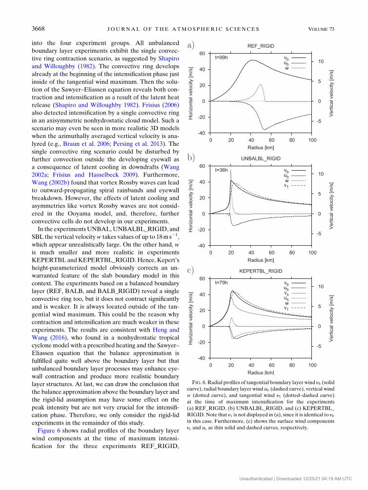
Figure 6 shows radial profiles of the boundary layer
wind components at the time of maximum intensi-
fication for the three experiments REF_RIGID,
FIG. 6. Radial profiles of tangential boundary layer wind yb (solid
curve), radial boundary layer wind ub (dashed curve), vertical wind
w (dotted curve), and tangential wind y1 (dotted–dashed curve)
at the time of maximum intensification for the experiments
(a) REF_RIGID, (b) UNBALBL_RIGID, and (c) KEPERTBL_
RIGID. Note that y1 is not displayed in (a), since it is identical to ybin this case. Furthermore, (c) shows the surface wind components
ys and us as thin solid and dashed curves, respectively.
3668 JOURNAL OF THE ATMOSPHER IC SC IENCES VOLUME 73
Unauthenticated | Downloaded 12/25/21 04:19 AM UTC

UNBALBL_RIGID, and KEPERTBL_RIGID. Note
that the tangential boundary layer wind in REF_
RIGID is identical to the gradient wind of the middle
model layer. In this simulation, the maximum inflow is
found at a radius of more than 50 km, while the
RMGW is located at a significantly smaller radius. This
has the consequence that the maximum vertical ve-
locity also lies at a radius larger than the RMGW. The
maximum inflow velocity of 36m s21 is very large, and
the resulting inflow angle of about 408 appears un-
realistically high (e.g., Frank 1977). In contrast, the
simulations UNBALBL_RIGID and KEPERTBL_
RIGID reveal a lower inflow angle, and the radius of
maximum inflow is close to the RMGW. Therefore, the
vertical wind peaks inside of this maximum. Further-
more, tangential winds become supergradient beneath
the developing eyewall in UNBALBL_RIGID and
also in KEPERTBL_RIGID but with a smaller am-
plitude in the latter. Experiment KEPERTBL_RIGID
has smaller horizontal wind shear inside of the tangential
wind maximum, and the peak vertical velocity is also
much smaller in comparison with UNBALBL_RIGID.
Boundary layer profiles similar to KEPERTBL_RIGID
were also observed in more complex cloud-resolving
models [e.g., Fig. 11a of Schecter (2011)]. We can also
clearly see weaker tangential winds at the surface, with
the consequence that the supergradient wind nearly
vanishes there, which is consistent with results found in
multilevel models [e.g., Fig. 10 of Bryan and Rotunno
(2009)]. The radial surface wind becomes weaker too at
most radii, but the reduction is smaller, and the radial
surface wind minimum is located more inward. Ooyama
found similar results in his unpublished work. In the
modified experiment conforming to experiment SBL, he
detected in comparison with the balanced model faster
intensification, RMGW contraction, a shift of the updraft
toward the center, and less expansion of theRMGWafter
the intensification phase. The smaller surface wind speed
considered in KEPERTBL_RIGID can explain the
slower intensification compared to UNBALBL_RIGID.
Indeed, the surface wind intensification rate might be
similar to that observed in the balanced boundary
layer simulation REF_RIGID. Therefore, the balanced
boundary layer model has, compared to a realistic model,
two deficiencies: (i) it overestimates the radius of eyewall
convection, and (ii) it overestimates the near-surface
wind speed. The experiments show that these two ef-
fects have opposing impacts. Profiles of UNBALBL_
RIGID and SBL_RIGID are almost identical at the time
of maximum intensification (not shown). Consequently,
the consideration of the local time tendency of boundary
layer momentum only enhances the amplification rate
but does not influence the radial wind structure. A
plausible candidate for explaining the differences to
REF_RIGID is the momentum advection term ub›ub/›r
in Eq. (3). It leads to higher inertia and more inward
intrusion of the inflow beyond the RMGW, where su-
pergradient winds and an updraft arise [for more dis-
cussion, see Frisius et al. (2013)]. This updraft lying
closer to the center provokes further contraction and
intensification, as will be shown in the next section.
However, the slab boundary model overestimates
the overshoot by inertia (Kepert 2010b). The height-
parameterized boundary layer model corrects this
overestimation to a high degree, but the inertia of the
inflow can still be important, since supergradient winds
also appear in KEPERTBL_RIGID.
4. Analysis of the intensification processes
O69 found conditional instability of the second kind
(CISK; Charney and Eliassen 1964) in his model by
linearizing the equations with respect to a conditionally
unstable atmosphere at rest. Growth due to CISK in-
creases with decreasing perturbation size. This property
is known as the ‘‘ultraviolet catastrophe’’ (Montgomery
et al. 2006) and leads to the consequence that only
horizontal diffusion can prevent shrinking of the per-
turbation to arbitrary small scales.4 However, the nu-
merical results are not inconsistent with such a scenario
indeed, since the width of the convective ring is close to
the scale of the grid and only remains finite because of
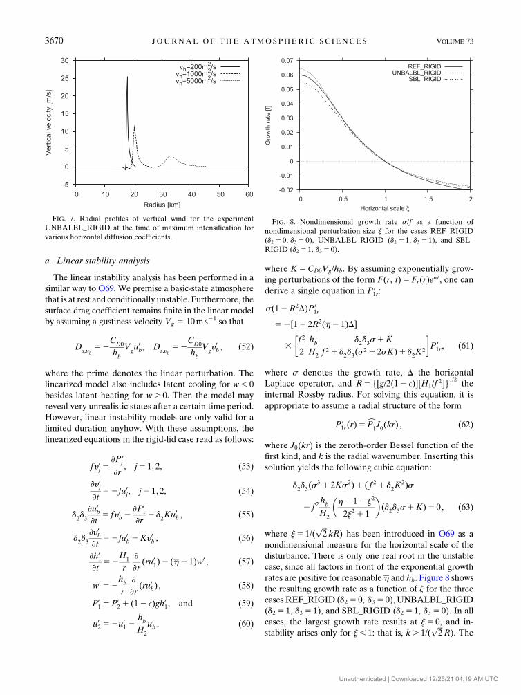
the inclusion of horizontal diffusion. The effect of hor-
izontal diffusion on the updraft profile in the in-
tensification phase for experiment UNBALBL_RIGID
is displayed in Fig. 7. Obviously, the width and radius
increases significantly with increasing horizontal diffu-
sion, while themaximum updraft velocity decreases. For
the low-diffusion case (nh 5 200m2 s21), a doubled grid
resolution was actually necessary to resolve the updraft
properly. This result is qualitatively consistent with
CISK, except for the difference that the updraft does not
develop at the vortex axis. On the other hand, Eliassen
(1971) showed that the updraft forms at a finite radius
when a quadratic drag law is used that is more similar to
that employed in the Ooyama model than a linear drag
law. Therefore, some aspects of intensification could
possibly be understood in terms of the CISK theory.
This possibility will be checked in the following.
4 It has to be noted that Charney and Eliassen (1964) found in
their CISKmodel rather uniform growth rates for disturbance sizes
smaller than about 100 km. Therefore, arbitrarily small distur-
bances grow only slightly faster than those having a scale of
about 100 km.
SEPTEMBER 2016 FR I S IU S AND LEE 3669
Unauthenticated | Downloaded 12/25/21 04:19 AM UTC
a. Linear stability analysis
The linear instability analysis has been performed in a
similar way to O69. We premise a basic-state atmosphere
that is at rest and conditionally unstable. Furthermore, the
surface drag coefficient remains finite in the linear model
by assuming a gustiness velocity Vg 5 10ms21 so that
Ds,ub
52C
D0
hb
Vgu0b, D
s,yb52
CD0
hb
Vgy0b , (52)
where the prime denotes the linear perturbation. The
linearized model also includes latent cooling for w, 0
besides latent heating for w. 0. Then the model may
reveal very unrealistic states after a certain time period.
However, linear instability models are only valid for a
limited duration anyhow. With these assumptions, the
linearized equations in the rigid-lid case read as follows:
f y0j 5›P 0
j
›r, j5 1; 2, (53)
›y0j›t
52fu0j, j5 1; 2, (54)
d2d3
›u0b
›t5 f y0b 2
›P01
›r2 d
2Ku0
b , (55)
d2d3
›y0b›t
52fu0b 2Ky0b , (56)
›h01
›t52
H1
r
›
›r(ru0
1)2 (h2 1)w0 , (57)
w0 52hb
r
›
›r(ru0
b) , (58)
P01 5P0
2 1 (12 �)gh01, and (59)
u02 52u0
1 2hb
H2
u0b , (60)
where K5CD0Vg/hb. By assuming exponentially grow-
ing perturbations of the form F(r, t)5Fr(r)est, one can
derive a single equation in P 01r:
s(12R2D)P 01r
52[11 2R2(h2 1)D]
3
�f 2
2
hb
H2
d2d3s1K
f 2 1 d2d3(s2 1 2sK)1 d
2K2
�P 01r, (61)
where s denotes the growth rate, D the horizontal
Laplace operator, and R5 f[g/2(12 �)][H1/f2]g1/2 the
internal Rossby radius. For solving this equation, it is
appropriate to assume a radial structure of the form
P 01r(r)5
cP1J0(kr) , (62)
where J0(kr) is the zeroth-order Bessel function of the
first kind, and k is the radial wavenumber. Inserting this
solution yields the following cubic equation:
d2d3(s3 1 2Ks2)1 ( f 2 1 d
2K2)s
2 f 2hb
H2
�h2 12 j2
2j2 1 1
�(d
2d3s1K)5 0, (63)
where j5 1/(ffiffiffi2
pkR) has been introduced in O69 as a
nondimensional measure for the horizontal scale of the
disturbance. There is only one real root in the unstable
case, since all factors in front of the exponential growth
rates are positive for reasonable h and hb. Figure 8 shows
the resulting growth rate as a function of j for the three
casesREF_RIGID (d2 5 0, d3 5 0), UNBALBL_RIGID
(d2 5 1, d3 5 1), and SBL_RIGID (d2 5 1, d3 5 0). In all
cases, the largest growth rate results at j5 0, and in-
stability arises only for j, 1: that is, k. 1/(ffiffiffi2
pR). The
FIG. 8. Nondimensional growth rate s/f as a function of
nondimensional perturbation size j for the cases REF_RIGID
(d2 5 0, d3 5 0), UNBALBL_RIGID (d2 5 1, d3 5 1), and SBL_
RIGID (d2 5 1, d3 5 0).
FIG. 7. Radial profiles of vertical wind for the experiment
UNBALBL_RIGID at the time of maximum intensification for
various horizontal diffusion coefficients.
3670 JOURNAL OF THE ATMOSPHER IC SC IENCES VOLUME 73
Unauthenticated | Downloaded 12/25/21 04:19 AM UTC

unstable modes have an updraft with the radius 2:4048/k
in the center, and the growth rate s increases with de-
creasing updraft diameter. The largest growth rates occur
for d2 5 1 and d3 5 1 (UNBALBL_RIGID). Therefore,
the inclusion of the local time tendencies ›u0b/›t and
›y0b/›t in UNBALBL_RIGID enhances the instability as
in the nonlinear experiments (see Fig. 4a). Equation (63)
simplifies drastically in the case d3 5 0 and has the fol-
lowing solution:
s5hb
H2
K
11 d2K2/f 2
h2 12 j2
2j2 1 1. (64)
For d2 5 0, this formula is very similar to that obtained by
O69 [see his Eq. (8.10)]. In his formula the additional
summand (12 �)j4 shows up in the denominator of the
second factor, but it has a small impact since 12 � � 1.
For d2 5 1, the growth rate becomes smaller than in the
case d2 5 0. Therefore, the violation of the balance as-
sumption in the steady boundary layer has a damping
effect in the linearized system. Thus, only nonlinear terms
in the boundary layer model can explain the larger in-
tensification rate observed in the nonlinear experi-
ments SBL_RIGID in comparison to REF_RIGID (see
Fig. 4a). This outcome does not appear surprising, since
the abovementioned radial momentum advection term
is not part of the linear model, and it is, therefore, un-
derstandable that it cannot explain the unbalanced
intensification phase properly. Furthermore, representa-
tion of a convective ring in terms of a Fourier–Bessel
series does not exhibit the ring contraction when each
coefficient growswith the corresponding growth rate (not
shown). Consequently, the linear model cannot explain
the contraction of the vortex either.
Further simulations have been performed in which the
vertically averaged radial momentum advection term
2u›u/›r has been set to zero in the boundary layer to
test if this term plays an important role for the inten-
sification. The experiments called SBLMOD_RIGIDand
KEPERTBLMOD_RIGID are identical to SBL_RIGID
and KEPERTBL_RIGID, respectively, except for this
modification. Figure 9 shows the maximum tangential
wind y1 and the RMGW for these additional simulations
as a function of time. The results for the unmodified runs
are also displayed for comparison. Obviously, the devel-
opment for SBLMOD_RIGID significantly differs from
that for SBL_RIGID. Both intensity and intensification
rate take much lower values than for SBL_RIGID. Fur-
thermore, the contraction of the RMGW already stops at
37km compared to the minimum RMGW of 12km ob-
served in SBL_RIGID. The final intensity is even lower
than in REF_RIGID. The omission of the radial mo-
mentum advection term has a visibly smaller effect in
Kepert’s height-parameterized boundary layer model, as
can be seen in Fig. 9b. This brings again intomind that the
slab boundary model overestimates the role of radial
momentum advection. We also performed simulations in
which both nonlinear advection terms 2u›u/›r and
2u›(y2 y1)/›r are omitted in the boundary layer and the
time tendencies are retained. In the case of a steady slab
boundary, these additional modifications have little ef-
fect, but neglecting 2u›(y2 y1)/›r reduces the intensifi-
cation and contraction by another significant amount in
Kepert’s height-parameterized boundary layer model.
These results demonstrate the vital role of nonlinear
momentum advection for intensification in the Ooyama
model. Possibly, nonlinear momentum advection in the
boundary layer could also explain some aspects of the
finite-amplitude nature of tropical cyclogenesis.5
b. Evaluation of the middle-layer momentum budget
The source termsBA,BB,BC,BD,BE, andBF [see Eqs.
(38)–(43)] cause a radial middle-layer flow, which in turn
FIG. 9. As in Fig. 2, but for (a) SBLMOD_RIGID and (b)
KEPERTBLMOD_RIGID (see text). The thin curves in (a) and
(b) show for comparison the results of the experiments SBL_
RIGID and KEPERTBL_RIGID, respectively.
5 Substantial intensification within 10 days occurs in UNBALBL_
RIGID only when the initial tangential wind maximum is above
3m s21 (not shown).
SEPTEMBER 2016 FR I S IU S AND LEE 3671
Unauthenticated | Downloaded 12/25/21 04:19 AM UTC

induces a tendency in tangential wind y1 through angular
momentum advection. Therefore, at least one of these
source terms should be responsible for intensification,
because the resulting radial flow should be inward to
produce a local increase of angular momentum. How-
ever, vertical transport of boundary layer air could also
contribute to a local increase of angular momentum,
but it appears rather unlikely that this process solely
accounts for intensification. Figure 10 displays the var-
ious contributions to the tendency of tangential wind y1as a function of radius and time for the experiment
UNBALBL_RIGID. As expected, latent heat (source
term BB) release provides the major contribution to
intensification and RMGW contraction. During the
contraction phase, it has a distinct and narrowmaximum
inside the RMGW. The small horizontal extension of
the response can be explained by the high inertial sta-
bility inside the RMGW where the maximum vertical
mass flux occurs (see Fig. 5). At the end of the con-
traction phase, nonnegligible contributions due to fric-
tional convergence (source term BA) and upper-layer
gradient wind change (source term BD 1BF) become
apparent. The former arises because of downward mo-
tion immediately inside of the eyewall leading to inward
flow in the middle layer. This descent could be an arti-
fact of the simple slab boundary layer model, since it
emerges with a much smaller amplitude in KEPERTBL_
RIGID (see Fig. 6). A corresponding upward flux from
the boundary layer into the middle layer does not ap-
pear, since the entrainment parameter h is larger than 1
below the eyewall, and, therefore, the updraft at the top
of the boundary layer transports air directly into the
upper layer [see Eqs. (11)–(13)]. The upper-layer gradi-
ent wind change contributes to the y1 tendency, since an
alteration of the radial pressure gradient in the upper
layer also modifies the radial pressure gradient in the
middle layer, leading to additional inflow. A relevant
process for upper-layer gradient wind intensification is
given by the vertical momentum flux Dy,y2 . However, a
large portion of this intensification is compensated by
outward advection of angularmomentum so that finally a
positive contribution remains, which is considerably
smaller than that of latent heat release. The impact of
upward momentum flux (source term BC) and diffusion
(source term BE) on midlevel inflow is negligible. Nev-
ertheless, both these processes also have a direct con-
tribution to the tangential momentum budget. Diffusion
mainly dampens intensification but also supports the
contraction of the RMGW. The direct tendency due to
upwardmomentum flux appears to be small compared to
latent heat release. All the displayed tendencies add up
to the total tendency (shown in Fig. 10h). The pattern
of the total tendency resembles that due to latent heat
release, but the radial extension of the maximum is
somewhat larger, which is mainly a consequence of hor-
izontal diffusion.
Figure 11 shows the middle-layer momentum budget
for experiment KEPERTBL_RIGID. In this experi-
ment, the entrainment parameter h remains above 1
during the complete simulation. Therefore, no shallow
convection and no momentum transport from the
boundary layer to the middle layer takes place. Conse-
quently, the tendencies due to upward momentum flux
vanish identically. The tendency due to frictional con-
vergence attains much smaller values, presumably be-
cause of the smaller vertical velocity at the top of the
boundary layer. The tendency due to horizontal diffusion
induces, in contrast to UNBALBL_RIGID, a spinup of
the tangential wind inside the RMGW but with a small
amplitude and after the vortex has already terminated its
contraction. The other tendency terms resemble quali-
tatively those of the experiment UNBALBL_RIGID.
However, the tendencies have a significantly smaller
amplitude, which explains the slower intensification in
KEPERTBL_RIGID.
Figure 12 displays the contributions to the tendencies
of y1 for the experiment REF_RIGID. Note that up-
wardmomentum flux out of the boundary layer does not
change the middle-layer tangential wind because in
REF_RIGID it is assumed that yb 5 y1. In contrast to
UNBALBL_RIGID, the tendency due to latent heat
release spreads over a larger radial range. This hap-
pens because the updraft has a larger width than in
UNBALBL_RIGID and is located outside of the
RMGW (see Fig. 5f), where a smaller inertial stability
occurs. Furthermore, the maximum tendency due to
heating is about a factor of 10 smaller compared to
UNBALBL_RIGID. Although the total heating might
be similar to UNBALBL_RIGID, the smaller peak
value can explain the smaller intensification rate in
REF_RIGID, since the radial gradient of latent heating
and not the total heating induces the gradient wind
increase [cf. Eq. (39)]. Frictional convergence only
dampens intensification in REF_RIGID, and its magni-
tude is very small. The upper-layer gradient wind change
contributes with a large amount to the midlevel inflow
in the mature stage. The radial flow induced by diffu-
sion also supports intensification in the mature stage,
but the resulting tendencies are very small. The direct
tendency due to diffusion is negative near the RMGW,
and, therefore, it mainly dampens intensification. After
maximum contraction, the RMGW migrates outward
rapidly. This happens because latent heat release pro-
duces a positive tangential tendency outside of the
RMGW, while frictional convergence decreases tan-
gential wind inside of the RMGW.
3672 JOURNAL OF THE ATMOSPHER IC SC IENCES VOLUME 73
Unauthenticated | Downloaded 12/25/21 04:19 AM UTC
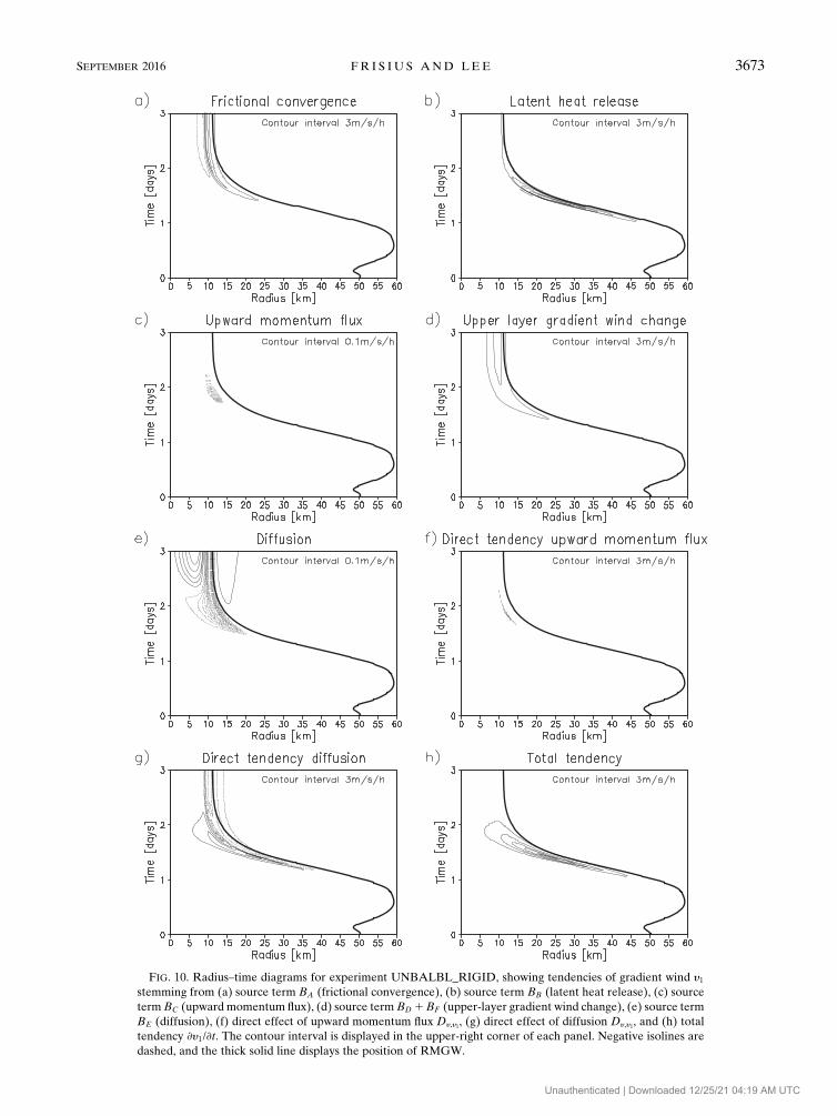
FIG. 10. Radius–time diagrams for experiment UNBALBL_RIGID, showing tendencies of gradient wind y1stemming from (a) source term BA (frictional convergence), (b) source term BB (latent heat release), (c) source
termBC (upward momentum flux), (d) source termBD 1BF (upper-layer gradient wind change), (e) source term
BE (diffusion), (f) direct effect of upward momentum flux Dy,y1, (g) direct effect of diffusion Dy,y1, and (h) total
tendency ›y1/›t. The contour interval is displayed in the upper-right corner of each panel. Negative isolines are
dashed, and the thick solid line displays the position of RMGW.
SEPTEMBER 2016 FR I S IU S AND LEE 3673
Unauthenticated | Downloaded 12/25/21 04:19 AM UTC

Comparison of Figs. 10 and 11 with Fig. 12 manifests
large qualitative and quantitative differences in the in-
tensification dynamics. In UNBALBL_RIGID and
KEPERTBL_RIGID the tendencies are mostly con-
centrated in a narrow ring inside of the RMGW, while in
REF_RIGID the tendency profiles are smoother and
sometimes are maximized outside the RMGW. The
reason for the different behavior of REF_RIGID is the
neglect of gradient wind imbalance in the boundary layer
model. The consequence is that the maximum ascent out
of the boundary layer occurs outside of the RMGWwith a
smooth radial profile (see Fig. 6a). This leads via latent
heat release to a gradient wind intensification with little
contraction and whose profile is also smooth.
To substantiate this conclusion further, steady-state
solutions of the unbalanced slab boundary layer model
and of Kepert’s height-parameterized boundary layer
model have been calculated using the gradient wind field
FIG. 11. Radius–time diagrams for experiment KEPERTBL_RIGID showing tendencies of gradient wind y1stemming from (a) source term BA (frictional convergence), (b) source term BB (latent heat release), (c) source
termBD 1BF (upper-layer gradient wind change), (d) source termBE (diffusion), (e) direct effect of diffusionDy,y1 ,
and (f) total tendency ›y1/›t. The contour interval is displayed in the upper-right corner of each panel. Negative
isolines are dashed, and the thick solid line displays the position of RMGW.
3674 JOURNAL OF THE ATMOSPHER IC SC IENCES VOLUME 73
Unauthenticated | Downloaded 12/25/21 04:19 AM UTC

of REF_RIGID at t 5 99 h. The results are shown in
Fig. 13, which should be compared with Fig. 6a. As ex-
pected, the boundary layer wind profiles differ greatly to
those of REF_RIGID. For the slab boundary layer
model, the vertical wind maximum arises far inside of
the RMGW, where strong supergradient winds are
found. The radial inflow also maximizes inside of the
RMGW and takes smaller values compared to the bal-
anced boundary layer calculation in REF_RIGID. The
steady-state solution of Kepert’s height-parameterized
boundary layer model also reveals an inward shift of the
vertical wind maximum and a decrease of the radial in-
flow velocity. However, the maximum vertical velocity
and the supergradient wind appear to be much smaller
than in the slab boundary layer model. Such differences
have already been noted and are consistent with the
findings of section 3. An inward shift of the frictional
updraft location was also found by Kepert (2013) with a
height-resolving boundary layer model when compared
with a linearized one. Furthermore, he demonstrated
that the linearized version yields vertical wind profiles
that resemble those found with the balanced slab
FIG. 12. As in Fig. 11, but for the experiment REF_RIGID.
SEPTEMBER 2016 FR I S IU S AND LEE 3675
Unauthenticated | Downloaded 12/25/21 04:19 AM UTC

boundary layer model of O69. Running the model by
using the gradient wind of REF_RIGID at t 5 99 h as
initial condition for d2 5 d3 5 1 would lead to immediate
contraction and rapid intensification. These results
support our conclusion on the importance of the non-
linear advection terms and show that it is of importance
for intensificationwhether the convective heating occurs
inside or outside of the RMGW.
5. Conclusions
In this study we have investigated the impact of the
balance assumption for the intensification of a tropical
cyclone in Ooyama’s three-layer model. Furthermore,
the effects of a rigid lid, the neglect of local time de-
rivatives in the boundary layer momentum equations,
and the inclusion of Kepert’s height-parameterized
boundary layer model have also been examined. We
found that the balance approximation in the two upper
layers and the rigid-lid assumption are of minor impor-
tance for the intensification phase, while the balance
approximation in the boundary layer has a significant
impact. With a balanced boundary layer (as given in ex-
periment REF_RIGID), the tropical cyclone intensifies
much more slowly than in the simulation employing
an unbalanced boundary layer (as given in experiment
UNBALBL_RIGID). Furthermore, the vortex contracts
only slightly during intensification, and the RMGW
increases dramatically after the intensity has maxi-
mized in REF_RIGID. In contrast, the simulation
UNBALBL_RIGID reveals a substantial vortex con-
traction with little RMGW variation after the intensi-
fication stage. In both experiments intensification is
accompanied by the occurrence of a convective ring in the
vicinity of the RMGW. However, in REF_RIGID the con-
vective ring is located outside and in UNBALBL_RIGID
inside the RMGW. We suggest that this discrepancy is
crucial for the different intensification rates. Because of
the higher inertial stability, latent heating inside the
RMGW leads to a larger and tighter tangential wind ten-
dency than in the case with heating outside the RMGW.
This can explain the faster growth and contraction in
UNBALBL_RIGID compared to REF_RIGID. An en-
hancement of intensification with increasing inertial sta-
bilitywas already foundbySchubert andHack (1982) in an
idealized analytical solution of the Sawyer–Eliassen
equation. This result hints at the importance of non-
linearity in tropical cyclone intensification, and the mech-
anismwas further elaborated byHack andSchubert (1986)
on the basis of nonlinear primitive equation and balanced
models. However, they assumed a time-independent heat
source, and, therefore, they excluded a possible feedback
of inertial stability on heating. This could stem from a
modification of the boundary layer inflow and the as-
sociated vertical mass fluxes. The results based on
Ooyama’s three-layer model show that the increasing
inflow in the unbalanced boundary layer supplies the
eyewall with enough moist air so that heating is main-
tained or even increased at larger inertial stability.
Eventually, the intensification stops because the fric-
tional dissipation rate increases at a much faster rate
than the energy input rate from the ocean (Wang 2012).
The simulations with neglected time derivatives (as
given in experiment SBL_RIGID) and with Kepert’s
height-parameterized boundary layer model (as given in
experiment KEPERTBL_RIGID) exhibit vortex con-
traction like in UNBALBL_RIGID, but the intensifica-
tion rates are smaller. Experiment KEPERTBL_RIGID
has more realistic wind profiles, and the smaller intensi-
fication rate in this experiment partially results because
the surface flux parameterization includes surface winds
FIG. 13. As in Fig. 6a, but the calculated boundary layer wind
profiles have been determined by finding the steady-state solutions
of (a) the unbalanced slab boundary layer model and (b) Kepert’s
height-parameterized boundary layer model.
3676 JOURNAL OF THE ATMOSPHER IC SC IENCES VOLUME 73
Unauthenticated | Downloaded 12/25/21 04:19 AM UTC

instead of vertically averaged winds, as in the slab bound-
ary layer model. Furthermore, the radial overshoot is
also reduced in the height-parameterized boundary
layer model (see Fig. 13) so that convection forms in a
less inertially stable environment, where a diminished
intensification rate results.
The linear instability analysis of the governing equa-
tions does not reveal an enhancement of the in-
tensification rate by the relaxation of the balance
assumption in the boundary layer, and it cannot ex-
plain the contraction of the intensifying vortex either.
Therefore, nonlinear terms appear to enhance intensi-
fication in the Ooyama model as a result of gradient
wind imbalance. The radial advection of radial mo-
mentum likely supports the intrusion of boundary layer
air inside of the RMGW, where the eyewall develops. A
simulation without this term in the slab boundary layer
model exhibits a much slower development with lit-
tle contraction. The reason for faster intensification
and contraction in UNBALBL_RIGID compared to
REF_RIGID has been found by analyzing the various
terms in the tangential wind equation of the middle
model layer. In both experiments latent heat release is
the main driver for intensification. Gradient wind
intensification by upward momentum flux from the
middle layer to the upper layer also contributes to in-
tensification in the middle layer in the later stages of
the development. The frictionally induced downdraft
inside the eyewall yields another contribution in
UNBALBL_RIGID. However, the crucial difference
between both experiments is the radial scale of the wind
tendency. In UNBALBL_RIGID the radial extent is
much smaller than in REF_RIGID because the eyewall
emerges in the inertially stable region inside of the
RMGW, while in REF_RIGID it arises outside of the
RMGW, where weak inertial stability dominates.
Although the intensification rate is smaller, experi-
ment KEPERTBL_RIGID reveals an intensification
mechanism resembling that of UNBALBL_RIGID.
Therefore, a more realistic representation of bound-
ary layer dynamics still supports the finding that gra-
dient wind imbalance in the boundary layer is of
importance for the intensification scenario and vortex
contraction.
These results suggest the following intensification
mechanism in Ooyama’s three-layer model. First, an
incipient vortex generates inflow, and the inflow over-
shoots the RMGW as a result of its inertia. The over-
shoot causes an updraft inside the RMGW, which
would occur outside the RMGW in the balanced and
the linearized boundary layer model [as found by
Kepert (2013)]. Then moist convective instability re-
leased by Ekman pumping generates a convective ring,
and the entrainment of air above the boundary layer
intensifies the tangential wind because of angular mo-
mentum import in the middle layer. Finally, the re-
sulting increase of gradient wind enhances the inflow
with more inward intrusion, which causes an inward
migration of the eyewall and further intensification.
Fluxes of latent heat from the sea surface are, of course,
necessary in this feedback loop to maintain the con-
vective instability near the eyewall radius. This picture
has some similarity with the CISK theory, since there is
also a cooperation of a large-scale vortex with con-
vection, and the latent heating depends on frictional
convergence in the boundary layer. However, the CISK
theory refers to an ensemble of individual convection
cells, but in the present model convection only appears
in the form of a single convective ring. Obviously,
convection is in the nonlinear Ooyama model only
triggered at the position where maximum frictional
convergence appears. Furthermore, the linear CISK
model by Charney and Eliassen (1964) predicts, like
the linearized Ooyama model, a maximum heating at
the vortex center, while in the nonlinear Ooyama
model it appears at a finite radius where the contracting
convective ring is located. This difference is in agree-
ment with the finding by Eliassen (1971) that a qua-
dratic drag law yields a boundary layer updraft
maximum at a finite radius. Ooyama (1982) already
appreciated the role of nonlinearities in his co-
operation intensification theory, but he did not con-
sider gradient wind imbalance in the boundary layer,
although he found previously in his unpublished study
that it enhances intensification. The frictionally in-
duced intensification mechanism is also consistent with
the study ofWang andXu (2010), who found in a cloud-
resolving model that inward boundary layer enthalpy
transport is important to the energy balance in the
eyewall.
The present study suggests that gradient wind imbal-
ance must be taken into account for a proper un-
derstanding of the intensification process. However, one
may ask why some balanced models already provide a
reasonable picture for intensification and vortex con-
traction. For example, Emanuel (1989) developed a
simple balanced hurricanemodel that reveals a behavior
as in the unbalanced case discussed here. On the other
hand, Emanuel (1989) applied a convective parameter-
ization scheme inwhich the convectivemass flux depends
directly on buoyancy and is independent of moisture
convergence in the boundary layer. Therefore, the
placement of the developing eyewall follows other rules
in his model than in the Ooyama model. A possible
drawback of the Ooyama model is the nonexistence of
ordinary conditional instability like that found by Lilly
SEPTEMBER 2016 FR I S IU S AND LEE 3677
Unauthenticated | Downloaded 12/25/21 04:19 AM UTC

(1960). Convective instability can take place without
frictional convergence in the boundary layer only if h
becomes unrealistically large. This is unlike the situation
in the vertically continuous atmosphere, where both
kinds of conditional instability occur simultaneously, if at
all (Fraedrich and McBride 1995). Possibly, convective
ring formation can result from ordinary conditional in-
stability in a more realistic model. This could potentially
explain why intensification and contraction arise without
surface drag in one of the axisymmetric model experi-
ments by Craig and Gray (1996). Such an outcome does
not invalidate the importance of unbalanced dynamics,
since ordinary convection cannot evolve in a balanced
model. Nevertheless, to reveal the relevance of the results
of the present study and the possible limitations of the
Ooyama model, it is necessary to investigate further the
intensification mechanism in more complex models.
Acknowledgments. This work was supported by the
Deutsche Forschungsgemeinschaft (DFG) within the
following individual research grant: The role of con-
vective available potential energy for tropical cyclone
intensification FR 1678/2-1. The first author also grate-
fully acknowledges support by the Cluster of Excellence
CliSAP (EXC177) funded by the DFG. We thank M. T.
Montgomery for the hint that K. V. Ooyama already
indicated the importance of unbalanced boundary layer
dynamics for intensification in an unpublished manu-
script that was kindly provided to us. Furthermore, we
thank three anonymous reviewers for their valuable
comments.
REFERENCES
Braun, S. A., M. T. Montgomery, and Z. Pu, 2006: High-resolution
simulation of Hurricane Bonnie (1998). Part I: The organiza-
tion of eyewall vertical motion. J. Atmos. Sci., 63, 19–42,
doi:10.1175/JAS3598.1.
Bryan, G. H., and R. Rotunno, 2009: Evaluation of an analytical
model for the maximum intensity of tropical cyclones.
J. Atmos. Sci., 66, 3042–3060, doi:10.1175/2009JAS3038.1.
Bui, H. H., R. K. Smith, M. T. Montgomery, and J. Peng, 2009:
Balanced and unbalanced aspects of tropical cyclone in-
tensification. Quart. J. Roy. Meteor. Soc., 135, 1715–1731,
doi:10.1002/qj.502.
Charney, J. G., and A. Eliassen, 1964: On the growth of the hur-
ricane depression. J. Atmos. Sci., 21, 68–75, doi:10.1175/
1520-0469(1964)021,0068:OTGOTH.2.0.CO;2.
Craig, G. C., and S. L. Gray, 1996: CISK or WISHE as the
mechanism for tropical cyclone intensification. J. Atmos.
Sci., 53, 3528–3540, doi:10.1175/1520-0469(1996)053,3528:
COWATM.2.0.CO;2.
DeMaria, M., and J. D. Pickle, 1988: A simplified system of
equations for simulation of tropical cyclones. J. Atmos. Sci.,
45, 1542–1554, doi:10.1175/1520-0469(1988)045,1542:
ASSOEF.2.0.CO;2.
Eliassen, A., 1971: On the Ekman layer in a circular vortex.
J. Meteor. Soc. Japan, 49, 784–789.
Emanuel, K. A., 1989: The finite-amplitude nature of tropical cy-
clogenesis. J. Atmos. Sci., 46, 3431–3456, doi:10.1175/
1520-0469(1989)046,3431:TFANOT.2.0.CO;2.
Fraedrich, K., and J. L. McBride, 1995: Large-scale convective
instability revisited. J. Atmos. Sci., 52, 1914–1923, doi:10.1175/
1520-0469(1995)052,1914:LSCIR.2.0.CO;2.
Frank, W. M., 1977: The storm structure and energetics of the trop-
ical cyclone. I: Storm structure.Mon.Wea. Rev., 105, 1119–1135,
doi:10.1175/1520-0493(1977)105,1119:TSAEOT.2.0.CO;2.
Frisius, T., 2006: Axisymmetric tropical cyclogenesis via a
single convective ring. 27th Conf. on Hurricanes and
Tropical Meteorology, Monterey, CA, Amer. Meteor. Soc.,
14B.7. [Available online at https://ams.confex.com/ams/
27Hurricanes/webprogram/Paper108695.html.]
——, 2015: What controls the size of a tropical cyclone? In-
vestigations with an axisymmetric model. Quart. J. Roy. Me-
teor. Soc., 141, 2457–2470, doi:10.1002/qj.2537.——, and T. Hasselbeck, 2009: The effect of latent cooling pro-
cesses in tropical cyclone simulations. Quart. J. Roy. Meteor.
Soc., 135, 1732–1749, doi:10.1002/qj.495.
——, D. Schönemann, and J. Vigh, 2013: The impact of gradient
wind imbalance on potential intensity of tropical cyclones in
an unbalanced slab boundary layer model. J. Atmos. Sci., 70,
1874–1890, doi:10.1175/JAS-D-12-0160.1.
Hack, J. J., and W. H. Schubert, 1986: Nonlinear response of
atmospheric vortices to heating by organized cumulus
convection. J. Atmos. Sci., 43, 1559–1573, doi:10.1175/
1520-0469(1986)043,1559:NROAVT.2.0.CO;2.
Hausman, S. A., K. V. Ooyama, and W. H. Schubert, 2006: Po-
tential vorticity structure of simulated hurricanes. J. Atmos.
Sci., 63, 87–108, doi:10.1175/JAS3601.1.
Heng, J., and Y. Wang, 2016: Nonlinear response of a tropical cy-
clone vortex to prescribed eyewall heating with and without
surface friction in TCM4: Implications for tropical cyclone
intensification. J. Atmos. Sci., 73, 1315–1333, doi:10.1175/
JAS-D-15-0164.1.
Hill, K. A., andG.M. Lackmann, 2009: Influence of environmental
humidity on tropical cyclone size. Mon. Wea. Rev., 137, 3294–
3315, doi:10.1175/2009MWR2679.1.
Kepert, J. D., 2010a: Slab- and height-resolving models of the
tropical cyclone boundary layer. Part I: Comparing the simu-
lations. Quart. J. Roy. Meteor. Soc., 136, 1686–1699,
doi:10.1002/qj.667.
——, 2010b: Slab- and height-resolving models of the tropical cyclone
boundary layer. Part II: Why the simulations differ.Quart. J. Roy.
Meteor. Soc., 136, 1700–1711, doi:10.1002/qj.685.
——, 2013: How does the boundary layer contribute to eyewall
replacement cycles in axisymmetric tropical cyclones?
J. Atmos. Sci., 70, 2808–2830, doi:10.1175/JAS-D-13-046.1.
Lilly, D. K., 1960: On the theory of disturbances in a conditionally
unstable atmosphere. Mon. Wea. Rev., 88, 1–17, doi:10.1175/
1520-0493(1960)088,0001:OTTODI.2.0.CO;2.
Montgomery, M. T., M. E. Nicholls, T. A. Cram, and A. B.
Saunders, 2006: A vortical hot tower route to tropical
cyclogenesis. J. Atmos. Sci., 63, 355–386, doi:10.1175/
JAS3604.1.
Ooyama, K. V., 1969: Numerical simulation of the life cycle of
tropical cyclones. J. Atmos. Sci., 26, 3–40, doi:10.1175/
1520-0469(1969)026,0003:NSOTLC.2.0.CO;2.
——, 1982: Conceptual evolution of the theory and modelling of
the tropical cyclone. J. Meteor. Soc. Japan, 60, 369–379.
3678 JOURNAL OF THE ATMOSPHER IC SC IENCES VOLUME 73
Unauthenticated | Downloaded 12/25/21 04:19 AM UTC

Persing, J., M. T. Montgomery, J. C. McWilliams, and R. K. Smith,
2013: Asymmetric and axisymmetric dynamics of tropical
cyclones. Atmos. Chem. Phys., 13, 12 299–12 341, doi:10.5194/
acp-13-12299-2013.
Schecter, D. A., 2011: Evaluation of a reduced model for in-
vestigating hurricane formation from turbulence. Quart.
J. Roy. Meteor. Soc., 137, 155–178, doi:10.1002/qj.729.
——, and T. J. Dunkerton, 2009: Hurricane formation in diabatic
Ekman turbulence. Quart. J. Roy. Meteor. Soc., 135, 823–838,
doi:10.1002/qj.405.
Schubert, W. H., and J. J. Hack, 1982: Inertial stability and tropical
cyclone development. J. Atmos. Sci., 39, 1687–1597,
doi:10.1175/1520-0469(1982)039,1687:ISATCD.2.0.CO;2.
Shapiro, L. J., andH. E.Willoughby, 1982: The response of balanced
hurricanes to local sources of heat and momentum. J. Atmos.
Sci., 39, 378–394, doi:10.1175/1520-0469(1982)039,0378:
TROBHT.2.0.CO;2.
Smith, R. K., and M. T. Montgomery, 2008: Balanced boundary
layers used in hurricane models. Quart. J. Roy. Meteor. Soc.,
134, 1385–1395, doi:10.1002/qj.296.
——, and ——, 2015: Toward clarity on understanding tropical cy-
clone intensification. J. Atmos. Sci., 72, 3020–3031, doi:10.1175/
JAS-D-15-0017.1.
——, G. Kilroy, and M. T. Montgomery, 2015: Why do model
tropical cyclones intensify more rapidly at low latitudes?
J. Atmos. Sci., 72, 1783–1804, doi:10.1175/JAS-D-14-0044.1.
Stern,D. P., J. L.Vigh,D. S.Nolan, andF.Zhang, 2015:Revisiting the
relationship between eyewall contraction and intensification.
J. Atmos. Sci., 72, 1283–1306, doi:10.1175/JAS-D-14-0261.1.
Wang, Y., 2002a: An explicit simulation of tropical cyclones
with a triply nested movable mesh primitive equation model:
TCM3. Part II: Model refinements and sensitivity to cloud
microphysics parameterization. Mon. Wea. Rev., 130, 3022–
3036, doi:10.1175/1520-0493(2002)130,3022:AESOTC.2.0.
CO;2.
——, 2002b: Vortex Rossby waves in a numerically simulated
tropical cyclone. Part II: The role in tropical cyclone struc-
ture and intensity change. J. Atmos. Sci., 59, 1239–1262,
doi:10.1175/1520-0469(2002)059,1239:VRWIAN.2.0.CO;2.
——, 2012: Recent research progress on tropical cyclone structure
and intensity.Trop. CycloneRes. Rev., 1, 254–275, doi:10.6057/
2012TCRR02.05.
——, and J. Xu, 2010: Energy production, frictional dissipation, and
maximum intensity of a numerically simulated tropical cyclone.
J. Atmos. Sci., 67, 97–116, doi:10.1175/2009JAS3143.1.
Williams, G., 2015: The effects of vortex structure and vortex trans-
lation on the tropical cyclone boundary layer wind field. J. Adv.
Model. Earth Syst., 7, 188–214, doi:10.1002/2013MS000299.
Xu, J., and Y. Wang, 2010: Sensitivity of the simulated tropical
cyclone inner-core size to the initial vortex size. Mon. Wea.
Rev., 138, 4135–4157, doi:10.1175/2010MWR3335.1.
SEPTEMBER 2016 FR I S IU S AND LEE 3679
Unauthenticated | Downloaded 12/25/21 04:19 AM UTC


