PROJECT NUMBER: TAC-MQP-FR20
The Effect of Substrate Variation on Biofilm Growth for Use in
Wastewater Treatment
A Major Qualifying Project
Submitted to the Faculty of
WORCESTER POLYTECHNIC INSTITUTE
in Partial Fulfillment of the Requirements for the
Degree of Bachelor of Science
Submitted by:
Sebastian Cohn
Alysia Hayes
Kristin Renault
Submitted to:
Project Advisors:
Prof. Terri Camesano
Prof. Destin Heilman
Site Advisor:
Prof. Marie Noelle Pons
April 8, 2010
2
Abstract
The formation of biofilms on surfaces exposed to water has had significant impacts on
wastewater treatment technology. Biofilms are used advantageously in wastewater treatment as
rotating biological contractors to degrade harmful organic and inorganic materials. However,
biofilm formation on equipment designed to inspect water quality, such as a passive sampler, can
alter calculated pollution concentrations. This project investigates the effect of salt and heavy
metals on a slowly rotating biological contactor and the effect of a strong magnetic field on a
quickly rotating biological contactor. The extent of biofouling on a passive sampler is also
examined. Opacity measurements are taken to measure biofilm accumulation. Biofilm efficiency
is monitored through Ultraviolet-Visible and Fluorescence Spectroscopy, the Ammonium Test,
and Ion Chromatography and heavy metal concentrations are measured with Inductively Coupled
Plasma Atomic Emission Spectroscopy.

3
Table of Contents
Authorship....................................................................................................................................... 7
Acknowledgments........................................................................................................................... 7
1 Summary ...................................................................................................................................... 8
2 Background ................................................................................................................................ 11
2.1 Wastewater Treatment........................................................................................................ 11
2.1.1 Components of Wastewater ......................................................................................... 11
2.1.1.1 Microorganisms .................................................................................................... 11
2.1.1.2 Biodegradable Organic Materials ......................................................................... 12
2.1.1.3 Organic Materials.................................................................................................. 12
2.1.1.4 Basic Nutrients ...................................................................................................... 13
2.1.1.4.1 Nitrogen Fixation ........................................................................................... 13
2.1.1.5 Metals & Inorganic Materials ............................................................................... 14
2.1.1.6 Other Factors ......................................................................................................... 14
2.1.2 Wastewater Treatment ................................................................................................. 15
2.1.2.1 Preliminary Treatment .......................................................................................... 15
2.1.2.2 Primary Treatment ................................................................................................ 16
2.1.2.3 Secondary Treatment ............................................................................................ 18
2.1.2.4 Advanced Treatment ............................................................................................. 20
2.2 Biofilms .............................................................................................................................. 21
2.2.1 Biofilm Structure ......................................................................................................... 22
2.2.1.1 The Biofilm Matrix ............................................................................................... 23
2.2.1.2 Microcolonies ....................................................................................................... 24
2.2.1.2.1 Horizontal Gene Transfer ............................................................................... 24
2.2.1.2.2 Quorum Sensing ............................................................................................. 25
2.2.2 Biofilm Formation ....................................................................................................... 25
2.2.3 Microbial Diversity...................................................................................................... 29
4
2.2.3.1 Bacteria ................................................................................................................. 29
2.2.3.2 Algae ..................................................................................................................... 30
2.2.3.3 Protozoa and Metazoa ........................................................................................... 31
2.3 Biofilm Applications .......................................................................................................... 32
2.3.1 The Effect of Salt and Heavy Metals on Biofilm Development .................................. 32
2.3.1.1 Chemical Properties of Seawater .......................................................................... 32
2.3.1.2 Biofilm Resistance to Heavy Metals..................................................................... 33
2.3.1.3 Research Application ............................................................................................ 34
2.3.2 The Effect of Biofouling on Passive Sampler Performance ........................................ 35
2.4 Analytical Techniques ........................................................................................................ 38
2.4.1 Fluorescence Spectroscopy .......................................................................................... 38
2.4.2 Ultraviolet Molecular Absorption Spectroscopy ......................................................... 39
2.4.3 Inductively Coupled Plasma Atomic Emission Spectroscopy (ICP-AES) .................. 41
2.4.4 Ion Exchange Chromatography ................................................................................... 44
2.4.5 Colorimetry: Ammonium Test .................................................................................... 44
3 Methodology ............................................................................................................................. 45
3.1 Experiment 1 ....................................................................................................................... 45
3.2 Experiment 2 ...................................................................................................................... 47
3.3 Experiment 3 ....................................................................................................................... 49
3.4 Analytical Techniques ........................................................................................................ 51
3.4.1 Opacity......................................................................................................................... 51
3.4.2 Fluorescence Spectroscopy .......................................................................................... 52
3.4.3 Ultraviolet-Visible Spectroscopy ................................................................................ 53
3.4.4 Ion Exchange Chromatography and the Ammonium Test .......................................... 53
3.4.5 Inductively Coupled Plasma Atomic Emission Spectroscopy (ICP-AES) .................. 55
4 Results ....................................................................................................................................... 55
4.1 Experiment 1 ...................................................................................................................... 55
4.1.1 Opacity......................................................................................................................... 55
4.1.3 Ultraviolet-Visible Spectroscopy ................................................................................ 61
4.1.4 Ion Chromatography and the Ammonium Test ........................................................... 64
4.1.5 ICP-AES Spectroscopy ................................................................................................ 67
5
4.2 Experiment 2 ...................................................................................................................... 69
4.2.1 Opacity......................................................................................................................... 69
4.2.2 Fluorescence Spectroscopy .......................................................................................... 72
4.2.3 Ultraviolet-Visible Spectroscopy ................................................................................ 73
4.2.4 Ion Chromatography and the Ammonium Test ........................................................... 75
4.3 Experiment 3 ....................................................................................................................... 79
4.3.1 Opacity......................................................................................................................... 79
4.3.2 Fluorescence Spectroscopy .......................................................................................... 83
4.3.3 Ultraviolet-Visible Spectroscopy ................................................................................ 84
4.3.4 Ion Chromatography and the Ammonium Test ........................................................... 86
5 Conclusions ............................................................................................................................... 88
5.1 Experiment 1 ...................................................................................................................... 88
5.2 Experiment 2 ...................................................................................................................... 91
5.3 Experiment 3 ...................................................................................................................... 92
6 Appendices ................................................................................................................................ 93
6.1 Procedures .......................................................................................................................... 93
6.1.1 Maintenance of the Biological Contactors .................................................................. 93
6.1.1.1 Procedure for the Maintenance of Experiment 1 .................................................. 93
6.1.1.1.1 Image of Experiment 1 Apparatus ................................................................. 95
6.1.1.2 Procedure for the Maintenance of Experiment 2 .................................................. 95
6.1.1.2.2 Image of Axle with Biofilm and Magnetic Discs .......................................... 97
6.1.1.3 Procedure for the Maintenance of Experiment 3 .................................................. 97
6.1.1.3.2 Image of the Horizontally Positoned Plastic Films on the Plate .................... 99
6.1.1.3.3 Image of the Plastic Films on the Plate in the Bottom of the Reactor ........... 99
6.1.1.3.4 Image of the Vertically Hanging Plastic Films .............................................. 99
6.1.2 Wastewater Substrate Preparation Procedure ............................................................ 100
6.1.2.1 Experiment 2 and 24 Substrate Preparation ........................................................ 100
6.1.2.2 Experiment 1 Substrate Preparation.................................................................... 100
6.1.3 Biofilm Scanning and Analysis ................................................................................. 101
6.1.3.1 Experiment 1 and Experiment 2 Biofilm Scanning ............................................ 101
6.1.5.2 Experiment 1 and Experiment 2 Analysis .......................................................... 102
6
6.1.5.3 Experiment 3 Biofilm Scanning.......................................................................... 103
6.1.5.4 Experiment 3 Analysis ........................................................................................ 104
6.1.6 Fluorescence Spectroscopy ........................................................................................ 106
6.1.7 Ultraviolet-Visible Spectroscopy .............................................................................. 107
6.1.8 The Ammonium Test ................................................................................................. 108
6.1.9 Ion chromatography ................................................................................................... 109
6.1.10 Inductively Coupled Plasma Atomic Emission Spectroscopy (ICP-AES) .............. 110
Work Cited .................................................................................................................................. 111
7
Authorship
This project was completed by Sebastian Cohn, Alysia Hayes, and Kristin Renault. The three
authors contributed equally to the laboratory work, research, and the writing of this report.
Acknowledgments
We would like to thank the following people for their guidance, support, and contributions
throughout this project:
Professor Terri Camesano, Worcester Polytechnic Institute, Project Advisor
Professor Destin Heilman, Worcester Polytechnic Institute, Project Co-Advisor
Professor Marie-Noelle Pons, ENSIC, Site Advisor
Muatasem Alnnasouri, ENSIC, Post Doctorate
Steve Pontvianne, ENSIC, Laboratory Technician

8
1 Summary
Effective and efficient water treatment are integral to a well-functioning society,
especially now, as natural water resources dwindle and contamination is becoming an
increasingly prominent issue. Before being returned to the natural environment or reused,
wastewater must go through a series of stages of treatment to purify the water and remove
materials that are potentially harmful to human health. In the final stages of this treatment, a
variety of methods are used to remove dangerous organic material and to denitrify ammonia
compounds present in the wastewater. Principal among these methods employs the use of
biofilm.
Biofilms are complex layers of microorganisms that coat surfaces exposed to water.
Biofilms consist of many different types of microorganisms, such as bacteria, fungi, algae, and
protozoa. The microorganisms colonize and excrete a matrix of extracellular polymeric
substance which encloses the biofilm and protects the microbial colonies from degradation,
predators, antimicrobials, and toxins. Biofilms remove organic and inorganic materials from the
surrounding water. This feature is used advantageously in wastewater treatment systems to
remove these harmful substances from the wastewater before it is reintroduced to the
environment.
While biofilms are often used beneficially to treat wastewater, they can also be a
nuisance and hazard. The development of biofilms generates many medical issues, including
dental plaque and the contamination of medical devices, and industrial problems, such as the
corrosion and clogging of water pipes. In addition, biofilms interfere with pollution monitoring
in wastewater treatment systems. Passive sampling is a technique used to monitor the
9
concentration of pollutants and toxins in a flowing water system. The pollutants are absorbed by
a plastic film and later excreted and analyzed to determine the level of pollution within the water
source. The growth of biofilm over the passive sampler, known as “biofouling”, prevents the
diffusion of the toxins into the passive sampler, resulting in inaccurately calculated toxin
concentrations.
This project examines the effectiveness and the resilience of biofilms on rotating disc
reactors under a variety of conditions. It also studies the extent of biofouling on two different
configurations of plastic films in a passive sampler with only dissolved oxygen as a source of
aeration. Three reactors were examined over a two month period using various analytical
techniques to measure the biofilm growth, the amount of protein in the reactor, the soluble
Chemical Oxygen Demand (COD), and the extent of nitrification occurring in the reactor. Each
reactor used equivalent volumes of wastewater and had equivalent water retention times.
The first reactor, Experiment 1, was a slowly rotating biological contactor in which
biofilm was grown upon five vertically oriented rotating discs. The discs were partially
submerged in a wastewater tank that was continually fed by a drip pump, feeding wastewater that
had been combined with salt and, later in the experiment, nickel ions. The purpose of the
experiment was to examine the effects of salt and heavy metals upon biofilm growth.
Wastewater samples were analyzed with Fluorescence Spectroscopy, UV-Visible Spectroscopy,
Ion Chromatography, and the Ammonium Test. The discs were scanned daily and analyzed using
a grayscale program to monitor biofilm accumulation. Finally, sludge and sloughed biofilm were
gathered weekly and tested using Inductively Coupled Plasma Atomic Emission Spectroscopy
(ICP-AES) to determine its heavy metal content. The experiment showed that the addition of salt
to the wastewater retarded the development of the biofilm and resulted in a thin and delicate

10
biofilm structure. The addition of nickel inhibited organic degradation, while also increasing
biomass.
The second experiment, Experiment 2, was a rotating biological contactor designed to
study the effects of a magnetic field in conjunction with a high rate of rotation upon biofilm
growth and longevity. In this experiment, two discs were placed inside of a high magnetic field
and two were placed outside of the magnetic field. The reactor was fed continually by a drip
pump feeding pure wastewater. As in Experiment 1, water samples were analyzed with
Fluorescence Spectroscopy, UV-Visible Spectroscopy, Ion Chromatography, and the
Ammonium Test. Daily scanning was also utilized in this test to determine the level of biomass
accumulation. The experiment demonstrated that the magnetic field and rotation speed affected
biomass accumulation and the rate of detachment. In addition, the results showed that the
magnetic field may have influenced the biodegradation of organic compounds and the initiation
of the nitrification process.
The final biological contactor, Experiment 3, was designed to examine the potential
effect of biofouling on long-term passive samplers to determine if different configurations of the
sampler would alter the extent of the biofouling. Sixteen rectangular films made from a plastic
garbage bag were placed into a reactor in two configurations: eight hanging vertically in the
water, and eight attached to a plate, which was horizontally positioned at the bottom of the
reactor. Both sets of films were evenly spaced in the tank, which was aspirated and fed with
wastewater. All of the films in the reactor were scanned for opacity in addition to being tested
with UV-Visible Spectroscopy, Fluorescence Spectroscopy, Ion Chromatography, and the
Ammonium Test. The conclusion reached was that the vertical orientation is the configuration in
a passive sampler that would be the least affected by biofouling.
11
2 Background
2.1 Wastewater Treatment
Modern wastewater treatment began in the early 1800s with the advent of the first
underground sewer system in London, followed shortly afterwards by similar ones in Paris,
Hamburg, and Chicago. However, while these removed wastewater, they did nothing to treat it
and reduce its toxicity, although the time spent in the sewer likely did induce a certain amount of
settling and other processes that unintentionally cleaned the water. Despite these new methods of
removing wastewater, an outbreak of cholera in London was eventually shown to be the result of
a pump contaminated by wastewater. This led to the discovery of a variety of water-borne
diseases and the understanding of the need for actual treatment of wastewater. Additional
discoveries and advancements in wastewater treatment over the past 150 years have made it
possible to reintroduce treated wastewater as potable water [1].
2.1.1 Components of Wastewater
The precise components of wastewater vary radically by location, and even by day within a
given location. Although wastewater comes primarily from three sources, industrial waste,
household waste, and runoff, the constituents of each of these sources are fundamentally
different. Their individual volumes may differ by location, time of day, and current weather (in
the case of runoff).
2.1.1.1 Microorganisms
12
The components that are found in wastewater can be divided into nine main groups.
Microorganisms may include pathogenic bacteria such as cryptosporidium, viruses, or worm
eggs. These are of particular concern to those dealing with water treatment as they have the most
immediate potential for causing illness. Although the vast majority of microorganisms are
harmless and found naturally in the human body, there are some mixed in that may cause disease
and so must be deactivated. This deactivation is the reason for the chlorination process that all
potable water goes through [2].
2.1.1.2 Biodegradable Organic Materials
Biodegradable organic materials make up another considerable part of wastewater. These
include such benign substances as pieces of bark, wood, and plant matter, in addition to feces
and animal matter that may have entered the wastewater through runoff or household waste
(dinner scrapings, etc). While they in and of themselves do not necessarily present a risk to the
environment, organic material tends to be the method by which microorganisms are conveyed.
While many microorganisms are water-born, they often are transmitted to the water through
organic material, so the removal of this organic material eliminates many of the microorganisms
[2].
2.1.1.3 Organic Materials
In addition to biodegradable organic material, wastewater contains a variety of other,
more basic, organic substances, including detergents, pesticides, fat, oil, grease, coloring,
solvents, phenol, and cyanide [2]. All of these must be removed, as they may be dangerous for
animal or human consumption. In recent years, the problem of dissolved pharmaceuticals in the
water has also come under scrutiny. Many of these are not removed effectively during the
13
treatment process, and those that are removed in sludge may not be broken down at all. This
means when the sludge is sold to farmers as a soil amendment the drugs infect the farmed
vegetation [3].
2.1.1.4 Basic Nutrients
Basic nutrients such as nitrogen, phosphorous, and ammonia are also found in
wastewater. These are of particular concern for the environment in which the wastewater is
released. Heavy nutrient loading in a natural water body results in the increased growth of
phytoplankton and opportunistic macroalgae well beyond the levels naturally found. Increased
levels of these organisms often leads to the reduction or disappearance of natural algal forms,
fewer plants within the water body, and changes in the composition of the water (including
reduced levels of dissolved O2). These changes all affect the animal ecosystems in and
surrounding the water body [4].
2.1.1.4.1 Nitrogen Fixation
Plants depend upon a variety of nutrients for growth, with nitrogen making up 1-10% of
their dry mass. In order to utilize the nitrogenous compounds found naturally, plants must go
through a process of nitrogen fixation [38]. Nitrogen fixation is performed by a variety of
bacteria found within the plant to convert nitrogen (often in the form of N2) into ammonia (NH3).
The plant may then use the ammonia as a source of energy and nitrogen necessary for cell-
growth. As previously explained, an abundance of nitrogen in the water promotes this process in
algal species that are harmful to the overall ecosystem in large numbers. In nature, excess
nitrogen may be removed given the proper conditions. For example, in wetlands, nitrogen
present in the water is converted into nitrogenous oxides before percolating into the soil. Since

14
wetland soil is continually flooded and therefore unable to be aerated and have significant levels
of O2, it is an anaerobic environment and promotes the denitrification process. Denitrification is
the method in which nitrogenous oxides are biologically reduced into N2O and N2 gas. Ideal
conditions for denitrification are found in wetland soil, in which there is an abundance of carbon
and a lack of oxygen [39]. In wastewater treatment, this same process is simulated in advanced
treatment and is discussed in section 2.1.2.4.
2.1.1.5 Metals & Inorganic Materials
The next two categories of materials found in wastewater, metals and other inorganic
materials (primarily acids and bases), are largely the result of industrial wastewater. While some
heavy metals are needed for both human and animal health (e.g. iron, copper, and zinc), these
levels are very small, generally far under the levels found in many industrial wastewater flows.
In addition, these flows often include metals such as lead and mercury whose ingestion will, over
time, cause significant adverse health effects. The inclusion of acids and bases in wastewater is
also of concern because of their effects upon the pH of the water. The pH is generally kept
within a certain range so as to avoid causing unnecessary problems in the environment in which
the treated water is released [2]
2.1.1.6 Other Factors
Other factors which affect wastewater include thermal effects, odor, and radioactivity.
First, thermal effects are important because oftentimes the wastewater entering a treatment plant
is substantially warmer than the water it will be released into. Aquatic ecosystems are often
extremely temperature-sensitive, making it necessary to bring the temperature of the treated
wastewater to within a defined percentage of the temperature of the water body it is being
15
released into. In addition, much of the foul odor emitted by wastewater is caused by sulfur in the
form of H2S, and so this must be removed as a part of odor control, which is particularly
important for treatment plants located in urban or suburban areas [5]. Finally, radioactivity can
be an issue if radioactive elements have been introduced to the wastewater. If an industrial
process is known to produce wastewater that is radioactive, then specific treatment processes
may be introduced either on-site or at the treatment facility that the wastewater goes to in order
to deal with the radioactivity [2].
2.1.2 Wastewater Treatment
In order to treat for all of these components, wastewater goes through four main stages of
treatment within a wastewater treatment facility: preliminary treatment, primary treatment,
secondary treatment, and advanced treatment. All of these provide some form of residuals, which
are in turn either incinerated or dried and added to soils as a supplement to be sold to farmers.
2.1.2.1 Preliminary Treatment
The primary purpose of preliminary treatment is to smooth out the stream so that the
later, more sensitive processes are not damaged. This may require the removal of larger objects
present in the wastewater flow or the hydraulics of the flow itself may need to be evened out,
with any surges removed. The first step of preliminary treatment is screening, in which the
wastewater flows through a screen or series of screens whose openings may range from 5 to 150
millimeters in order to filter out larger debris in the water. These screens may be manually
cleaned or cleaned mechanically, in which chain- or cable-driven “teeth” rake the screen
regularly to remove debris. Once the larger debris has been captured and removed it is sent
through a grinder to be turned into a more manageable size. Grinders use two sets of
16
intermeshing cutters to reduce solids to sizes between six and nine millimeters. Once ground
down, the screenings will generally be treated as municipal trash and will be sent to a municipal
landfill or incinerated at a municipal incinerator. If the township dealing with the waste requires
it, the screenings may sometimes need to be washed and dried before being incinerated [7].
Once the larger objects have been removed, the wastewater goes through a process of grit
removal, which is accomplished through different settlers. Grit may consist of sand, gravel, other
mineral matter, and certain organics including coffee grounds, egg shells, and seeds. It can be
removed simply through short-term settling, or in a settling tank, in which minor turbulence is
introduced to the system so that lighter organic particles remain suspended while the heavier grit
is removed. The importance of removing grit during preliminary treatment is to avoid the wear it
causes upon mechanical systems of the wastewater treatment plant, in addition to buildup and
accumulation of grit inside of anaerobic digesters and biological reactors [7].
The final purpose of preliminary treatment is that of equalization. Equalization may refer
to flow or waste-strength. Both of these must be made steady to ensure a constant level and
quality of effluent without risk to the more sensitive apparatuses at later stages of treatment. This
is achieved through the use of “equalization tanks”, large tanks that store water and release it
over time at a steady rate, so that spikes in flow or strength of contaminants are minimized
through release over an extended period of time [7].
2.1.2.2 Primary Treatment
Primary treatment is the oldest form of wastewater treatment, and removes the vast
majority of organics and contaminants from the wastewater. In primary treatment the water goes
through a process of coagulation and flocculation followed by settling in order to, in conjunction
with scraping, remove much of the organic material from the wastewater. The idea behind

17
coagulation and flocculation is that many of the particles that must be removed from the water
are small enough that they are suspended, and will never settle to the bottom of the tank or rise to
the surface, or at least not in a timely manner. Therefore, they are chemically induced to become
attractive to one another and form clumps, which have sufficient mass to sink during the settling
process [7].
The first step of primary treatment is preaerating the wastewater. Increasing the dissolved
O2 levels of the water helps promote flocculation in addition to improving the floating tendencies
of scum in the water, so that it can more easily be scraped off in the settling tanks. Next, the
water goes through the process of coagulation. While material will settle out of the water and be
removed without it, coagulation has been shown to increase the amount of material that settles,
depending upon the source of wastewater, by upwards of 50%. Coagulants commonly used
include aluminum salts, iron salts, and lime, although aluminum sulfate, or “alum” is likely the
most common coagulant being used today [6]. All of these reverse the polarity of some of the
particles, causing them to become attracted to one another, and to clump together. However, if
excessive amounts of coagulant are added, it will fully reverse the polarity of the colloid
complex in the wastewater and result in a total lack of clumping [7].
Once the coagulant has been added, the water must go through a short “rapid mix”
process in order to ensure that the colloid is completely dispersed throughout the water. After
this has been completed, the water moves on to a “slow-mix tank” in which it continues to be
mixed, but at a rate designed to induce flocculation of the suspended solids. Often there are
several stages of slow mixing, with the mixing becoming slower and gentler at each stage so as
to avoid breaking up the flocs [7].
18
The second half of primary treatment is settling. In the settling tank the water travels
extremely slowly, with minimal turbulence being created so that particles in the water may settle
to the bottom of the tank and be removed as sludge. This is achieved through the use of a moving
scraper that shovels the sludge into a hopper. In addition, scum is continuously scraped off of the
top of the settling tank in much the same manner as sludge is scraped from the bottom. Once
removed, the sludge and scum may either be disposed of or dried and used as soil additives.
Another option that is becoming more popular is to capture the methane gas that is released from
the sludge during the drying process and use it to generate a small amount of electricity. The
plant then utilizes the electricity generated to offset its own energy costs [7].
2.1.2.3 Secondary Treatment
Secondary treatment may be classified as two distinct systems: suspended growth or
fixed-film systems. Regardless of the precise method by which they go through the process, both
systems serve the same purpose: to remove any residual biological content in the wastewater
after it has gone through primary treatment. Suspended growth and fixed-film systems may each
be further broken down into several specific types of reactors. Reactors that operate via a
suspended growth system include activated sludge systems, aerated lagoons, and aerobic
digestion systems. Fixed-film systems, however, include trickling filters, rotating biological
contactors (similar to those being studied in this report), and packed-bed reactors [8].
Activated sludge is the oldest and most commonly used form of secondary treatment. It
was developed in America in the early 1900’s and involves the mixing of microorganisms (or
“activated sludge”) that can stabilize organics found in wastewater while mechanically bubbling
air through the system in order to create an aerobic environment. These microorganisms are
19
continually mixed with the water and air for a set amount of time, growing in number through
the consumption of organics, and forming floc particles of 50 to 200 micrometers, large enough
to precipitate out of the water. In the next step the floc is settled out in a secondary clarifier, and
a portion is recycled as activated sludge. This may be carried out as a batch process or as
continual flow. Using this method, the biological reactor typically removes over 99% of the
suspended solids present in the wastewater after primary treatment [8].
The most common fixed-film system is the “trickling filter”. This is also a type of aerobic
reactor, but it uses a continually grown biofilm rather than recycled activated sludge as its
biological agent. Trickling filters are towers of packed, specialized plastic m material, in which
approximately 90% to 95% of the volume of the tower remains as void space. The wastewater is
then sprayed over the top of the tower, from which point it trickles down through the packing
material. As a result of the constant flow of wastewater and supply of oxygen, which is provided
by either natural drafts or blowers, a biofilm grows upon the packing material. The biofilm
consumes the organics present in the wastewater. Occasional sloughing of the biofilm does
occur, which is then collected in the bottom of the reactor and removed as waste sludge. As with
the activated sludge system, the wastewater leaving the reactor goes through a secondary clarifier
to settle out any remaining pieces of biomass [8].
Rotating biological contactors (RBCs) use the same principles as trickling filters in that
they are also fixed-film reactors. However, in RBCs the biological film is grown upon discs that
rotate, entering and leaving the wastewater. This action allows the water to flow down the
biofilm and be treated as the disc as it rotates out of the water. In addition, continually leaving
the water provides air for the biofilm, so that it may act as an aerobic reactor. As in the trickling
filter, the biofilm on RBCs does occasionally slough off, and so must be collected and removed

20
as sludge. However, unlike trickling filters, the biofilm sloughs off due to sheer forces in
addition to its own weight, which does not allow for thick biofilm growth. One advantage of
RBCs is that they are entirely visible and may be easily monitored and repaired if necessary [8]
Also, the frequency of sloughing, and hence thickness of the biofilm, may be controlled by
modifying the speed of rotation of the reactor. In fixed film systems, modifying the flow velocity
of water moving through the reactor is the only way to alter this variable [40].
2.1.2.4 Advanced Treatment
The final stage of wastewater treatment is “advanced treatment”. While there is no single
process that defines advanced treatment, it may be described as “any process designed to
produce an effluent of higher quality than normally achieved by secondary treatment processes
or containing unit operations not normally found in Secondary Treatment” [9]. This is of course,
a rather broad definition. However, as advanced treatment is meant to remove anything that the
other forms of treatment miss, there are several distinct components of the wastewater that are
generally being removed in advanced treatment. While it may remove any remaining vestiges of
organic material, advanced treatment is often designed for nutrient removal (nitrogen,
phosphorous, and ammonia) and the removal of non-organic toxic substances, often of the sort
introduced to the wastewater by industrial sources. While levels of Biochemical Oxygen
Demand (BOD) are almost always reduced to acceptable levels through primary and secondary
treatment, the use of advanced treatment allows wastewater to be recycled. The treated water
may be used for the domestic water supply, for use in industrial situations, or simply to dilute the
inbound flow of untreated wastewater if there are dangerously high levels of pollutants [9].

21
Although the removal of toxins often requires specific treatment techniques for each type of
toxin being removed, one form of advanced treatment that is often used is biological
denitrification. The purpose of this treatment is to convert ammonia present in the water to
nitrate, thus satisfying the Nitrogenous Oxygen Demand (NOD). Without this conversion,
bacteria may use ammonia as their own energy source, converting it to nitrate and nitrite, and
using this energy to reproduce. Biological denitrification is carried out by keeping the
wastewater in an anaerobic environment and mixing a carbon source (generally methanol) with
it. The carbon allows for sufficient cell-growth of controlled nitrogen-consuming bacteria in the
anaerobic environment. Once these cells have consumed the available ammonia, the water goes
through a process of clarification and filtration to remove the cell colonies. Providing a proper
amount of methanol (or other carbon source) is key, as any excess will remain in the effluent.
Also important for this process is to maintain the pH between 6.0 and 8.0 and to keep track of the
temperature, as denitrification rates vary greatly with temperature. For example, denitrification
occurs five times faster in 20ºC water than in 10ºC water, and so retention time must be varied
accordingly [9].
2.2 Biofilms
Throughout history microorganisms have commonly been classified in the planktonic form,
freely floating and suspended in an aqueous medium. It was not until Van Leeuwenhoek
observed that microbial cells aggregate on tooth surfaces that microbial biofilms were
discovered. Later, other scientists determined that microbial attachment to a surface enhances
growth and that bacteria tend to congregate on surfaces instead of freely moving in the
surrounding environment. Finally, the development of scanning and transmission electron
22
microscopy enabled scientists to ascertain the composition of the biofilm and the surrounding
matrix material [10].
A biofilm is an aggregation of microorganisms irreversibly attached to a solid surface and
enclosed by a matrix of extracellular polymeric substance [10]. Biofilms can consist of many
different types of microorganisms, such as bacteria, diatoms, fungi, algae, and protozoa, and
noncellular materials, such as salt or silt. Biofilms are located on solid materials in an aqueous
medium and acquire organic and inorganic material floating in surrounding water. Organic
compounds, such as nitrogen and phosphorous and reduced inorganic compounds provide energy
for the metabolism of the biofilm [11].
Research pertaining to biofilms has increasingly become important to medicine, industry, and
the environment. Medically, biofilms can contaminate implanted biomedical devices and infect
living tissues. The extracellular surface of the biofilm conveys increased resistance to antibiotics
and other treatments. Dental plaque, a leading cause of cavities, is also a biofilm. In industry,
biofilms clog and corrode pipes resulting in damaged equipment and contamination. Biofilms are
used advantageously as biofilters, which control air pollution by passing odorous air through a
filter containing microorganisms that treat the air and remove the odor. Finally, in municipal and
industrial wastewater treatment systems, biofilms are used to remove the harmful organic and
inorganic material [12].
2.2.1 Biofilm Structure
The structure of biofilms varies but certain structural characteristics are common among all
biofilms. All biofilms are composed of microcolonies of bacterial cells embedded in a matrix of
extracellular polymeric substance. Hydrodynamic channels separate the microcolonies from one

23
another and provide means of communication between the bacterial cells and permit the
diffusion of nutrients, oxygen, and detritus. Differences in biofilm structure arise from alterations
to the biofilm due to the microorganisms that encompass the biofilm, the presence of external
forces, hydrodynamic conditions, nutrient availability, and particle interactions with noncellular
elements from the surrounding environment [10]. For example, biofilms grown in fresh water
exhibit thicker and denser channels than biofilms grown in salt water [16].
2.2.1.1 The Biofilm Matrix
The biofilm matrix encloses the bacteria and determines the architecture and shape of the
biofilm. Extracellular polymeric substance (EPS) is the major component of the biofilms’s
matrix and comprises 50% to 90% of the total organic carbon of the biofilm. Although the
physical and chemical properties of the EPS of different biofilms may vary, the principal
component of all EPS is polysaccharides. The polysaccharides of the EPS acquire great
quantities of water through hydrogen bonding resulting in a highly hydrated matrix composed of
97% water [13]. The synthesis of EPS relies of the availability of nutrients. EPS synthesis is
promoted by an excess of carbon and an inadequacy of other nutrients, such as nitrogen and
phosphate. EPS production is also stimulated by inhibited bacterial growth [16].
The composition of the exopolysaccharides in different bacterial strains may vary. The
polysaccharides of the EPS matrix of gram negative bacteria are neutral or polyanionic because
of the presence of uronic acids. These polysaccharides are drawn to divalent cations, which
subsequently crosslink the polymer strands and strengthen the biofilm. In contrast, the
polysaccharides comprising the matrix of gram positive bacteria produce polycationic EPS [10].
The structure of the biofilm matrix is also dependent upon the attachment of polysaccharides to
24
hydrophobic groups. Hydrophobic groups, such as methyl, contribute to cell surface
hydrophobicity. In addition, the presence of 1-3 or 1-4 beta linked hexose residues establishes
greater rigidness and lowers the solubility of the biofilm [16].
The polysaccharides that comprise the matrix give a three dimensional shape to the
mature biofilm and provide structural support. The matrix enables the bacterial cells to remain
close to the surface and to easily attach to one another [10]. In addition to the structural function
of the biofilm matrix, another main function of the matrix is to provide protection. The hydrated
layer of EPS prevents the biofilm from dehydration and enables the embedded cells to avoid
recognition by immune systems, resulting in biofilm resistance to antimicrobials. The matrix also
serves as barrier against the diffusion of toxins into the biofilm and protects the biofilm from
predators [13].
2.2.1.2 Microcolonies
The basic building block of the biofilm is the microcolony. The microcolonized structure
of biofilms and the water channels separating the colonies enable the cells to be in close
proximity to each other. The close proximity is required for the exchange of genes through
conjugation and stable cell to cell signaling [16].
2.2.1.2.1 Horizontal Gene Transfer
Horizontal gene transfer through bacterial conjugation is the method in which bacteria are
able to transfer DNA to bacterial organisms other than their descendants. Extrachromosomal
DNA is exchanged through conjugation at a greater rate in biofilms than in freely drifting
bacterial cells. Conjugation is the favorable method of gene transfer in biofilms because of
closer cell to cell contact, minimal shear forces, greater nutrient availability, and the stabilization

25
of the cells on the substratum. The F conjugative pilus of the bacterial donor cell produced by
the tra operon, or the transfer gene cluster operon, of the F plasmid directs the attachment of the
bacterial donor cell to a recipient cell. DNA is passed from the donor to the recipient organism
through the pilus resulting in biofilm formation and expansion [10].
2.2.1.2.2 Quorum Sensing
Quorum sensing, or cell to cell signaling, is essential to biofilm development. Experiments
with the bacteria P. aeruginosa showed that a minimum of one cell signaling system is necessary
for normal biofilm development. There are two cell to cell signaling systems involved in P.
aeruginosa biofilm formation, lasR-lasD, which regulates virulence and directs the second
system, rH 1R-rH 1I, which controls the production of secondary metabolites [17]. Mutants
lacking both cell signaling systems are unable to produce a biofilm. Mutants lacking one cell
signaling system are able to produce a biofilm, but the structural assembly is thinner and more
densely packed than the wild type. In addition, the mutant lacks the typical water channels that
separate the microcolonies in the wildtype biofilm and the biofilm is easily removed by
surfactant [10].
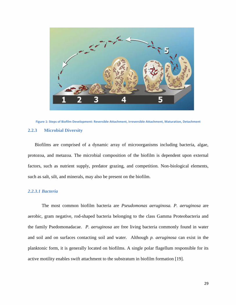
2.2.2 Biofilm Formation
Biofilm formation involves a series of distinct stages consisting of reversible attachment,
irreversible attachment, maturation, and detachment. Biofilm attachment begins at the solid-
liquid interface of the surface and aqueous surroundings. First, the bacteria weakly associate
with the surface through Van der Walls forces. In order to make this attachment, the bacteria
must overcome various repulsive forces at the solid-liquid interface, such as electrostatic
repulsion and hydrophobic interactions [15]. Substratum effects, the conditioning film,
26
hydrodynamic strength, and other characteristics of the aqueous medium and cell surface enable
the bacteria to overcome these repulsive forces and establish the initial reversible attachment.
Several substratum effects of the solid surface appear to influence the effectiveness of the
attachment and the ability of the bacteria to overcome the repulsive forces. First, attachment is
enhanced by increased surface roughness which minimizes shear forces and increases surface
area. Microorganisms also attach more competently and quickly to hydrophobic, nonpolar
surfaces than hydrophilic, polar surfaces [10]. In addition, the exposure of the solid surface to
the aqueous surroundings results in the adsorption of proteins, glycoproteins, proteoglycons, and
polysaccharides leading to the formation of the conditioning film. The adsorption of these
molecules enables the initial attachment through chemical modifications of the interface, such as
the changes in electric charge and hydrophobicity [11].
Hydrodynamic strength also greatly affects microbial adhesion to the solid-liquid interface
by acting as a repulsive or attractive force and thereby influencing the rate of the attachment. A
hydrodynamic boundary exists in the area of the interface where there is an insignificant flow
velocity. The thickness of the boundary layer is dependent upon the linear velocity rates and the
shear forces of the surrounding aqueous medium [10]. Greater linear velocities and high shear
force results in thinner boundary layers, denser biofilms, and more rapid union with the surface.
Low linear velocities and smaller shear forces produce thicker boundary layers and result in
slower attachment. A greater linear velocity of the liquid enables the cells to more efficiently
cross the boundary and attach to the surface [11].
Attachment to a surface is also affected by characteristics of the surrounding aqueous
medium. Temporal variations such as seasonal effects, unrelated aquatic environments, nutrient
27
composition and concentration, temperature, pH, and the strength of ionic interactions may affect
the rate of microbial adhesion [10].
Properties of the cell that affect attachment include hydrophobicity, appendages that enable
motility, lipopolysaccharide (LPS), and extracellular polymeric substance (EPS). Hydrophobic
constituents exist on the fimbrae of many bacteria and enable the bacteria to overcome
electrostatic repulsions at the interface and attach to hydrophobic surfaces [10]. Flagella assist
bacterial cells in their movement across the hydrodynamic boundary at the solid liquid interface
and facilitate attachment to a surface. The motile function of flagella appears to serve as a
propeller to translocate the cells as well as an adhesive appendage to attach the cell to the
substrate [11]. LPS is important to attachment because organisms that lack the O polysaccharide
of LPS are unable to effectively attach to a substrate. The O antigen supplies hydrophilic
properties to gram-negative bacteria enabling reversible attachment to hydrophilic surfaces [15].
EPS is integral to reversible attachment because the polyhydroxyl groups of the polysaccharides
associated with EPS in the biofilm matrix anchor the bacteria to the surface through hydrogen
bonding.
If the conditions for reversible attachment are favorable, the bacteria are able to engage in a
more secure attachment through reorientation to the surface resulting in irreversible attachment.
If the conditions were unfavorable and the bacteria were unable to reversibly attach to the
surface, the bacteria reenter the planktonic state. During irreversible attachment, the orientation
of the bacteria changes and the bacteria is longitudinally bound to the surface. Current research
has demonstrated that the cytoplasmic protein SadB may be responsible for regulating
irreversible attachment. In addition, a large adhesion, Lap A associates with the bacterial cell
28
envelope and an ABC transporter. Bacteria lacking Lap A are unable to advance past reversible
attachment [15].
The next step of biofilm formation is maturation, or the three dimensional growth of the
biofilm. Following irreversible attachment, the bacteria begin to grow and aggregate into
microcolonies. More planktonic bacteria are recruited and additional microorganisms colonize.
As the bacteria cultivate, extracellular polymers are produced and the bacteria become embedded
in a highly hydrated matrix [16]. The microcolonies in the EPS matrix are separated by water
channels and pores that are necessary for the diffusion of nutrients, oxygen, and debris within the
biofilm. The hydrodynamic voids also enable the cells to communicate with one another
through the exchange genes and quorum sensing [14].
The final step of biofilm growth, detachment, results from the shedding of cells, changes in
the environment, and physical forces. The shedding of cells can be attributed to cellular lysis,
the release of progeny, and the discharge of single cells in planktonic form that could not attach
to the biofilm. Hydrodynamic forces and the velocity of the liquid result in the natural erosion of
the biofilm, or shearing, in which small segments of the biofilm are constantly eliminated.
Abrasion can also cause detachment through collision of liquid particles with the biofilm.
Sloughing, in which large portions of the biofilm rapidly separate, is caused by depletions in
nutrients or oxygen availability. The thickness of the biofilm is dependent upon the net buildup
of the cells through attachment and maturation and the net loss of cells through detachment.
Research has shown that the rate of detachment escalates as the thickness of the biofilm
increases [14].
29
Figure 1: Steps of Biofilm Development: Reversible Attachment, Irreversible Attachment, Maturation, Detachment
2.2.3 Microbial Diversity
Biofilms are comprised of a dynamic array of microorganisms including bacteria, algae,
protozoa, and metazoa. The microbial composition of the biofilm is dependent upon external
factors, such as nutrient supply, predator grazing, and competition. Non-biological elements,
such as salt, silt, and minerals, may also be present on the biofilm.
2.2.3.1 Bacteria
The most common biofilm bacteria are Pseudomonas aeruginosa. P. aeruginosa are
aerobic, gram negative, rod-shaped bacteria belonging to the class Gamma Proteobacteria and
the family Psedomonadacae. P. aeruginosa are free living bacteria commonly found in water
and soil and on surfaces contacting soil and water. Although p. aeruginosa can exist in the
planktonic form, it is generally located on biofilms. A single polar flagellum responsible for its
active motility enables swift attachment to the substratum in biofilm formation [19].
30
Several characteristics of p. aeruginosa contribute to its ability to thrive on biofilms.
First, p. aeruginosa can grow in the absence of oxygen if nitrate is available to act as an electron
acceptor. In addition, the nutritional needs of p. aeruginosa are minimal and the bacteria can
utilize more than seventy-five organic compounds for growth. P. aeruginosa is able to grow on
mediums containing acetate as a source of carbon and ammonium sulfate as a source of nitrogen.
P. aeruginosa can withstand extreme physical conditions and flourishes at temperatures ranging
from 37 to 42 degrees Celsius. Finally, P. aeruginosa is resistant to many antimicrobials and can
endure high concentrations of salt [19].
A study of biofilm formation of thirteen bacterial strains found in wastewater treatment
systems showed that all thirteen bacterial strains were able to form biofilms on at least one of the
four different media used. Three of the strains, Pseudomonas aeruginosa, Acinetobacter
calcoaceticus, and Comamonas denitrificans, were able to form biofilms on any of the tested
media. Several adherence characteristics, including cell surface hydrophobicity, hydrodynamic
strength, initial attachment, and the production of EPS, contributed to the bacteria’s affinity to
form biofilms [20].
2.2.3.2 Algae
Diatoms, the unicellular algae of the class Bacillariophyceae, are the earliest and most
extensive colonizers of biofilms. They live in fresh and salt water and constitute a large portion
of marine plankton. Frustules, or firm bivalve shells composed of silica, and chloroplasts, enable
diatoms to perform photosynthesis. Diatoms attach to the surfaces of biofilms through a variety
of adhesive mechanisms, including filaments, glue-like substances, pads, and stalks. Once a few
31
cells have attached to the biofilm, cell division quickly results in colonization and the merging of
the microcolonies [18].
Unicellular and filamentous green algae and blue-green algae contribute to biofilms in
freshwater environments. Blue green algae, or cyanobacteria, are photosynthetic bacterium of the
class Coccogoneae. Cyanobacteria may exist as individual cells, filaments, or colonies and are
capable of nitrogen fixation. The ability of cyanobacteria to withstand extreme temperatures and
to utilize nitrogen fixation in the case of oxygen or nutrient deprivation contributes to their
flourishing existence on biofilms.
Algal biofilms are also present in marine environments. Enteromorpha, green algae that
grow as tubular single layer of cells, and Ectocarpus, small brown algae that form branched
filaments, produce flagellate zoospores and adhesive rhizoids that assist in the initial attachment
of the algae to the substratum [18].
2.2.3.3 Protozoa and Metazoa
The grazing of protozoa and metazoa alters the composition and nutrient supply of the
biofilm. Protozoa remove 30% to 100% of the bacteria produced each day within the biofilm.
The protozoa are grazed on by invertebrates, such as rotifers and nematodes. This food chain
results in the cycling of carbon, nitrogen, and phosphorous and the excretion of ammonia and
orthophosphate [16]. In addition, studies have shown that the channels present between the
microcolonies may be attributed to the movement and grazing of protozoa and metazoa [21].
Protozoa are single-celled eukaryotic organisms, belonging to the kingdom Protista, that
associate with biofilms and graze on bacteria and algae. They are nonphotosynthetic organisms
that exist singularly or aggregate into colonies. Protozoa are classified as amoebae, flagellates,
32
or ciliates according to their motility and means to capture prey. The level of attachment and
grazing varies among the different classes of protozoa. Primarily planktonic, or “transient
protozoa” do not directly attach to the biofilm. “Sessile protozoa” attach the surface but also
consume prey in the surrounding environment. Finally, the remaining protozoa principally use
the biofilm as a source of nourishment [16].
Metazoan invertebrates utilize bacteria and protozoa as an important food source and thereby
become common components of biofilms. Rotifers, multicellular organisms of the phylum
Rotifera, are the most common invertebrate in biofilms. Rotifers feed on bacteria by filtering
water passing the biofilm surface. They also graze on sessile ciliates by migrating into the
biofilm. Nematodes, unsegmented worms of the phylum Nematoda, are able to live inside the
biofilm matrix and graze on bacteria, amoebae, and sessile ciliates. Through the consumption of
dead cells, rotifers and nematodes enable growth and the proliferation of new cells in the biofilm
[21].
2.3 Biofilm Applications
2.3.1 The Effect of Salt and Heavy Metals on Biofilm Development
2.3.1.1 Chemical Properties of Seawater
Salinity, temperature, pH, and the dissolved gas and nutrient composition of seawater
affect biofilm development in marine environments. Seawater is made up of water and various
dissolved chemical elements and salts. The salinity of seawater in the majority of marine
environments is 35 parts per thousand. Chloride, sodium, sulfur, magnesium, calcium and
potassium comprise 99% of the salts found in seawater. Although the salinity of seawater may
fluctuate, these salts are always found in the same proportions. Evaporation, precipitation, water
33
runoff from streams and rivers, and the freezing and thawing of ice all affect salinity and biofilm
formation [42].
The temperature of seawater also varies with respect to the amount of sunlight it receives
and the angle of the sun’s rays. Tropical environments may present seawater temperatures as
high as 30 degrees Celsius, while polar environments may exhibit temperatures as low as -2
degrees Celsius [42]. Studies have shown that water temperatures from 2 to 7 degrees Celsius
and from 20 to 25 degrees Celsius resulted in a slow rate of biofilm maturation and production.
Maximal biofilm formation occurred at a seawater temperature of 15 degrees Celsius. In
addition, salinity and temperature affect the density of the seawater, which may affect the vitality
of marine microbes [43].
Finally, the concentration of dissolved gases and nutrient composition of seawater may
fluctuate in different marine environments. The amount of dissolved oxygen and carbon dioxide
in the seawater is dependent upon the temperature and types of organisms found in the aquatic
surroundings. Decreased temperature elevates the concentration of dissolved gases and the
photosynthetic activity of plants increases oxygen levels. The availability of nutrients is also
dependent upon the inhabitation and decomposition of organisms in the seawater. The nutrient
composition of seawater is important to biofilm formation because organic compounds, such as
nitrogen and phosphate, and reduced inorganic compounds provide energy for the metabolism of
the biofilm and promote or impede the synthesis of EPS [42].
2.3.1.2 Biofilm Resistance to Heavy Metals
Heavy metals, such as nickel, copper, and lead, are unrelenting pollutants of drinking
water, wastewater, freshwater, and marine environments. Heavy metals have extremely adverse
34
effects on human health, including DNA damage from free radicals and the breakdown of the
protein folding mechanisms. Biofilm bacteria, such as P. aeruginosa, possess intrinsic methods
to resist heavy metal toxicity. Biofilms are capable of eliminating heavy metals from the
surrounding liquid by binding the heavy metal ions to the EPS matrix. The use of biofilms in
wastewater treatment facilities has been investigated as a method of removing heavy metal from
wastewater [44].
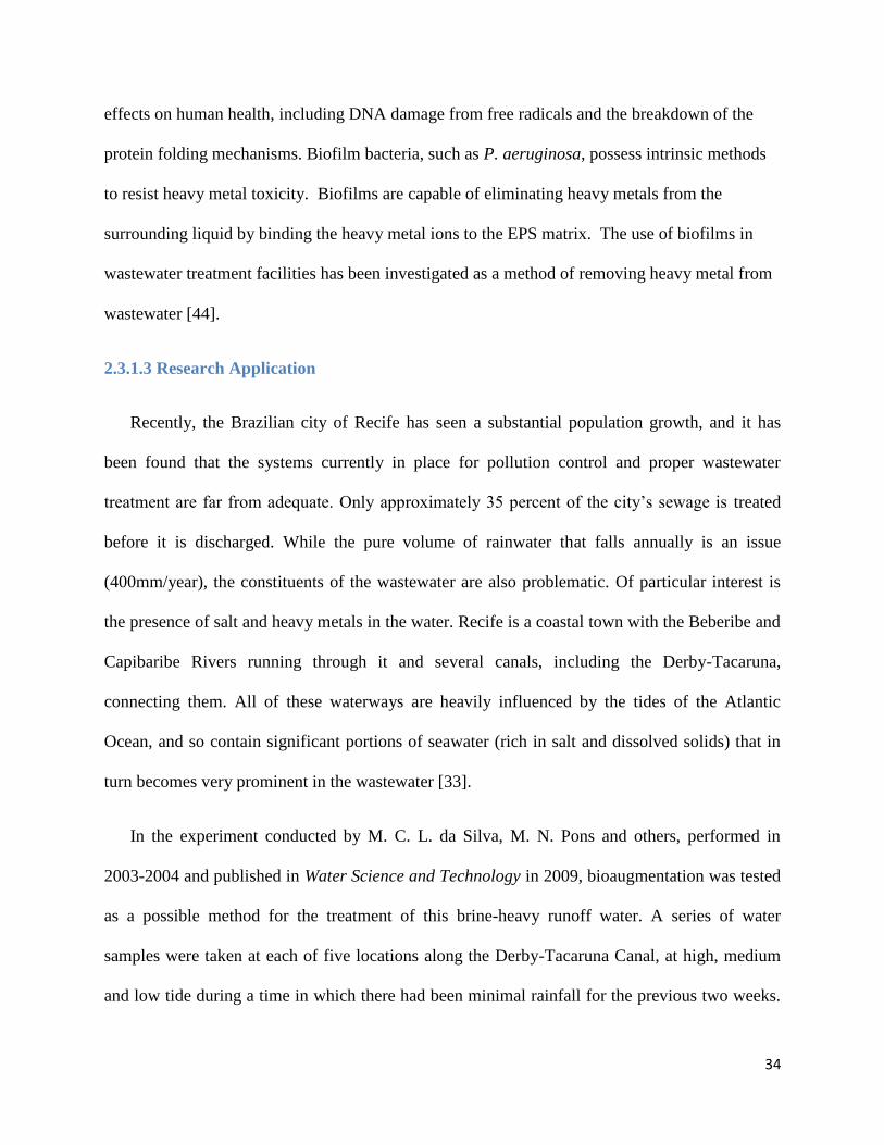
2.3.1.3 Research Application
Recently, the Brazilian city of Recife has seen a substantial population growth, and it has
been found that the systems currently in place for pollution control and proper wastewater
treatment are far from adequate. Only approximately 35 percent of the city’s sewage is treated
before it is discharged. While the pure volume of rainwater that falls annually is an issue
(400mm/year), the constituents of the wastewater are also problematic. Of particular interest is
the presence of salt and heavy metals in the water. Recife is a coastal town with the Beberibe and
Capibaribe Rivers running through it and several canals, including the Derby-Tacaruna,
connecting them. All of these waterways are heavily influenced by the tides of the Atlantic
Ocean, and so contain significant portions of seawater (rich in salt and dissolved solids) that in
turn becomes very prominent in the wastewater [33].
In the experiment conducted by M. C. L. da Silva, M. N. Pons and others, performed in
2003-2004 and published in Water Science and Technology in 2009, bioaugmentation was tested
as a possible method for the treatment of this brine-heavy runoff water. A series of water
samples were taken at each of five locations along the Derby-Tacaruna Canal, at high, medium
and low tide during a time in which there had been minimal rainfall for the previous two weeks.
35
These samples were then tested for a variety of parameters, after which one representative
sample was sent through a reactor using activated sludge and “bioaugmentation”. In
bioaugmentation a commercial bioadditive containing a variety of lyophilized strains of bacteria
is added to the wastewater prior to treatment as a replacement for activated sludge. Within this
reactor the mixture was aerated via perforated tube, while being sampled at five different points
throughout the reactor. These samples were then tested for the same parameters as the water had
been prior to treatment [33].
The data obtained by this experiment showed several results. First, the high levels of bacteria
in the unprocessed canal water confirmed previous observations of substantial amounts of
untreated wastewater being released into the waterways of the area. In addition, it was confirmed
that the high levels of salinity, conductivity, and dissolved solids are due largely to the tide, as all
were generally highest in the samples taken at high tide. Heavy metals were also present in the
untreated water, with Iron and Lead having particularly high concentrations. Results showed that
the bioaugmentation was substantially less efficient at removing both BOD and COD than the
traditional activated sludge system. Bioaugmentation removed 55% and 62% of COD and BOD
on average, respectively. Activated sludge, however, removed 89% and 96.8% of COD and
BOD, respectively [33].
2.3.2 The Effect of Biofouling on Passive Sampler Performance
Passive sampling is a technique used to monitor the concentration of organic and
inorganic pollutants in low concentrations and to assess water quality. Older grab sampling
techniques utilize bottle samples to record pollutant concentrations at specific time intervals.
However, these techniques are susceptible to variations in the pollutant concentrations in natural
36
waters. Limitations to the grab sampling method arise from fluctuations of contaminant
concentrations over time and the intermittency of pollution events. However, the technique of
passive sampling is well equipped to monitor time dependent concentrations of pollutants and is
not as sensitive to the innate variations of the aqueous environment. The greater stability of
passive sampling results in more reliable data for the long term monitoring of pollutants. In
addition, passive sampling reduces electricity usage and is thereby is the most cost-effective
method. Over the past twenty years, passive sampling technology has greatly advanced and is
becoming an increasingly more common method of pollution monitoring in water treatment
facilities [34].
Passive sampling is based on the free flow of analyte molecules from the sample medium
to the receiving phase in another medium due to a difference in the chemical potentials of the
analyte of the two media. The analyte molecules continue to flow between the media until
equilibrium is established. This results in the isolation of the analyte molecules in the receiving
phase of the passive sampler. The absorbed analyte molecules in the passive sampler can then be
dissolved and analyzed [35].
Different types of passive samplers are used to acquire information about pollution
concentrations. Linear, or non-equilibrium, passive samplers do not reach equilibrium within a
sampling period. These types of samplers have a high capacity for collecting target pollutants
over the entire sampling period, providing the time-weighted average of the concentration of
pollutants over a specific period of time. Another type of passive samplers, equilibrium passive
samplers, are not used to determine the time-weighted average because the equilibrium times of
different passive samplers may differ. Instead, equilibrium passive samplers signify the level of

37
the pollutant contamination in the monitored section. Contaminants pass through a sorption
medium and are trapped in the receiving medium inside in the sampler [35].
Environmental conditions and biofouling can greatly affect passive sampler performance.
Surfaces submerged in water become colonized by bacteria and other microorganisms resulting
in the formation of a biofilm. Biofilms reduce the sampling uptake rate of the passive sampler
by increasing resistance to mass transfer of contaminants from the water to the receiver. The
resistance to mass transfer is caused by an increased barrier thickness and blockage of pores. In
addition, certain microorganisms are capable of biodegradation, resulting in the decomposition
of analytes in the water that contact the biofilm surface and subsequently the miscalculation of
the concentration of pollutants [36].
Current research has been completed to measure the effect of biofouling on uptake rate in
passive samplers and two main approaches have been utilized to examine the biofouling effect.
The first method entails the biofouling of a membrane and the measurement of the sampling
uptake rates of the contaminants. The second method involves the addition of triolein to
compounds in the passive sampler. The differences in the release rates of the compounds are then
related to differences in biofouling. Richardson et al. experimented with biofouled membranes
and the addition of triolein to compounds in coastal waters over a four week period. The results
of the experiment showed that biofouling reduces contaminant uptake by fifty percent.
Additional research by Huckins et al. implies that the addition of organic solvents and pesticides
may reduce biofouling [37].
38
2.4 Analytical Techniques
2.4.1 Fluorescence Spectroscopy
Fluorescence is a specific type of photoluminescence, the general term used to describe the
interaction that occurs when molecules are excited by the absorption of photons of
electromagnetic radiation and then, consequently, the re-emission of light energy. The
phenomenon of fluorescence occurs when a beam of light is passed through a sample and the
photons of light excite the electrons of the molecules in the sample. The electrons jump into
higher energy molecular orbitals and then as they fall back into their original orbitals they emit
energy in the form of light. Fluorescence is characterized by this almost immediate re-emission
of energy after absorption, the entire event occurring in only 10-12
to 10-9
second [22].
Fluorescence can be measured through the use of a fluorescence spectrometer. A typical
instrument consists of a radiation source, a primary monochromator, a secondary
monochromator, a detector, an amplifier, and a readout device. Light from the source of radiation
is passed through the primary monochromator, which allows only the wavelength of light
required for excitation of the molecules in the sample to pass through. The second
monochromator, located at a 90° angle from the incident optical path, absorbs this primary
radiant energy, transmitting only the fluorescent radiant energy. The geometrical arrangement of
this device makes it particularly sensitive, around three to four orders of magnitude more
sensitive than the spectrophotometer, and therefore a very important analytical tool [23].
In biological and biochemical fields of study, the fluorescence spectrometer is often used to
detect fluorescent probes. There are three classes into which fluorescent probes can be divided:
intrinsic probes, extrinsic covalently bonded probes, and extrinsic associating probes.

39
Tryptophan is one of the three aromatic amino acid residues found in proteins which act as
intrinsic fluorophores (the other two amino acids being tyrosine and phenylalanine)[24] and
although typical proteins are comprised of only 1.1 molar percent tryptophan residues, this
particular amino acid is a very valuable probe of protein structure [25]. In comparison to the
absorption maxima (λmax) and extinction coefficient (ε) for both tyrosine (λmax=274.8, ε=1405)
and phenylalanine (λmax=257.6, ε=195), tryptophan has a higher wavelength of absorption and a
much higher extinction coefficient (λmax=279.0, ε=5579). Both of these factors contribute to the
dominance of the tryptophan emission signal, making it the “ultimate energy acceptor in
proteins” [23]. For this reason, tryptophan can be used as a fluorescent probe to determine the
relative concentrations of protein, and hence of organic materials, contained within different
samples of wastewater.
2.4.2 Ultraviolet Molecular Absorption Spectroscopy
In the process of electronic excitation, the electrons of a molecule, originally found at the
lowest energy state, the ground state, absorb radiant energy and move into higher energy states.
In order for radiation to cause this electronic excitation, it must be in UV region of the
electromagnetic spectrum. The near-UV (quartz) region of the electromagnetic spectrum, which
extends from 200 to 380 nanometers, is the main area of focus in ultraviolet spectroscopy.
In the case of organic molecules there are three different types of electrons separated into two
categories: bonding electrons and nonbonding electrons. The energy required to excite the
electrons involved in saturated hydrocarbon bonds (one σ bond) is often more than that which
UV light produces, and hence paraffinic compounds are quite useful as solvents. The electrons
found in unsaturated hydrocarbon bonds (such as those found in aromatics and conjugated

40
olefins), which usually contain one σ bond and one π bond, are capable of being excited by UV
radiation. For this reason, these electrons, as well as those not involved in bonding (n electrons),
may absorb UV radiation. N electrons are found in organic compounds containing nitrogen,
oxygen, sulfur or halogens. Functional groups that contain electrons which can absorb radiation
in the UV region are known as chromophores [29]. Wastewater contains both nitrate (-ONO2),
which has an absorption peak around 220 nm, and nitrite (-ONO), which has an absorption peak
at 270 nm [30].
Another important parameter used when analyzing wastewater which can be determined
using the UV-Vis spectrophotometer is the COD. The Chemical Oxygen Demand is a measure of
the amount of organic material within a given sample of water, or effluent in general, which is
susceptible to chemical oxidation. The standard method employed in the determination of COD
involves a variety of toxic chemicals and takes several days; hence many scientists have begun to
seek new analytical techniques to employ. The UV-Vis spectrophotometer can be used to
estimate the COD of a sample based on the fact that the organic materials in the effluent show
well-known absorption peaks in the UV-Visible region of the electromagnetic spectrum. These
peaks result from the incorporation of absorbing groups, such as aromatic compounds [30]. In a
previous study, conducted by Mrkva in 1975, a correlation between this organic matter in natural
waters and the UV absorbance at 254 nm was discovered and using this particular wavelength
allows for the estimation of the COD [31].
Absorption is detected using a device called an ultraviolet/visible spectrophotometer. This
device uses two light sources: a tungsten lamp for visible light and a deuterium lamp for
ultraviolet light. The beam of radiation from the light sources is divided into its component
wavelengths by a prism or diffraction grating. Each monochromatic beam of light is then divided
41
into two identical beams of light by a half-mirrored device. One of the beams of light passes
through the sample cell, a quartz cuvette containing the sample being studied dissolved in a
solvent, while the other passes through a reference cell. After passing through these cells, the
intensities of the two beams of light are then compared. The difference in the intensities gives a
direct measure of the absorption by the sample [29].
2.4.3 Inductively Coupled Plasma Atomic Emission Spectroscopy (ICP-AES)
Inductively coupled plasma atomic emission spectroscopy (ICP-AES) is one of the most
commonly employed analytical techniques because it is capable of detecting trace amounts,
typically 1-10 parts per billion, of many trace elements. Similar to atomic emission spectrometry,
in ICP technology samples are decomposed to their elemental components inside high
temperature argon plasma, the atomic constituents being excited to higher energy levels. These
components are then analyzed based on the wavelength of light their electrons emit when
returning to their ground states. ICP-AES involves four main processes: sample introduction and
aerosol generation, ionization of specific elements by argon plasma, separation of light emitted
by atoms into characteristic wavelengths, and quantification of each sample calibrated against
standards [41].
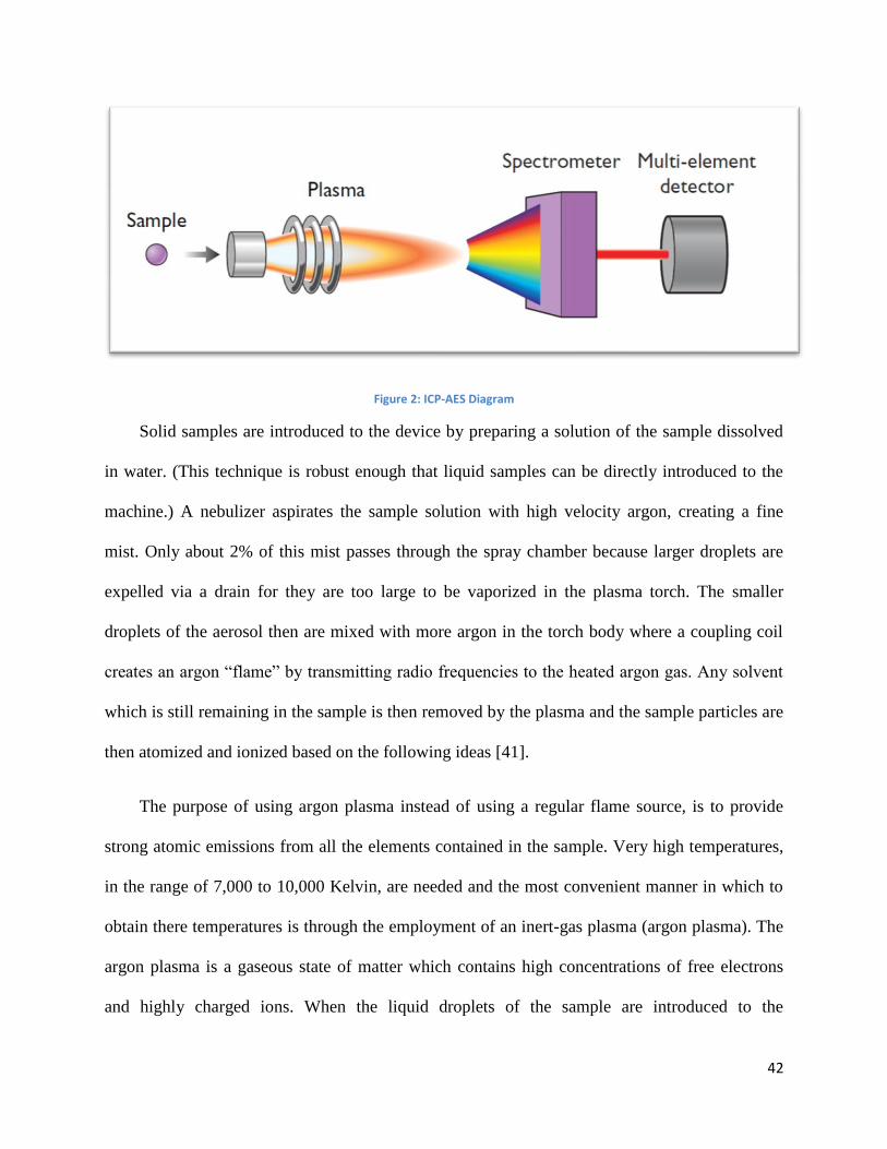
42
Figure 2: ICP-AES Diagram
Solid samples are introduced to the device by preparing a solution of the sample dissolved
in water. (This technique is robust enough that liquid samples can be directly introduced to the
machine.) A nebulizer aspirates the sample solution with high velocity argon, creating a fine
mist. Only about 2% of this mist passes through the spray chamber because larger droplets are
expelled via a drain for they are too large to be vaporized in the plasma torch. The smaller
droplets of the aerosol then are mixed with more argon in the torch body where a coupling coil
creates an argon “flame” by transmitting radio frequencies to the heated argon gas. Any solvent
which is still remaining in the sample is then removed by the plasma and the sample particles are
then atomized and ionized based on the following ideas [41].
The purpose of using argon plasma instead of using a regular flame source, is to provide
strong atomic emissions from all the elements contained in the sample. Very high temperatures,
in the range of 7,000 to 10,000 Kelvin, are needed and the most convenient manner in which to
obtain there temperatures is through the employment of an inert-gas plasma (argon plasma). The
argon plasma is a gaseous state of matter which contains high concentrations of free electrons
and highly charged ions. When the liquid droplets of the sample are introduced to the
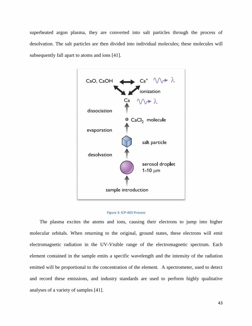
43
superheated argon plasma, they are converted into salt particles through the process of
desolvation. The salt particles are then divided into individual molecules; these molecules will
subsequently fall apart to atoms and ions [41].
Figure 3: ICP-AES Process
The plasma excites the atoms and ions, causing their electrons to jump into higher
molecular orbitals. When returning to the original, ground states, these electrons will emit
electromagnetic radiation in the UV-Visible range of the electromagnetic spectrum. Each
element contained in the sample emits a specific wavelength and the intensity of the radiation
emitted will be proportional to the concentration of the element. A spectrometer, used to detect
and record these emissions, and industry standards are used to perform highly qualitative
analyses of a variety of samples [41].
44
2.4.4 Ion Exchange Chromatography
Natural and artificial zeolites (sodium aluminum silicates) have been used for many years to
remove calcium and magnesium ions from water because they include metal ions, which are able
to exchange places with the other metal ions. Ion exchangers are now being produced which
combine a polymer (a resin which acts as an insoluble inert support) and a functional group,
which dictates whether the exchanger is anionic or cationic. Acids are usually used as the
functional group in cation exchange resins while amines or quaternary ammonium salts are
generally used in anion exchange resins.8 Both types of exchangers can be used for the
analyzation of wastewater, the dominant ions being Cl-, NO2
-, NO3
-, PO4
-3, and NH4
+ [29].
The rate of ion exchange, and hence separation of the ions, is governed by their relative
affinities. The metal ions in the sample are in constant competition for binding of the functional
groups. Generally at equal concentrations the ion with the highest affinity for the functional
group will take the binding site and move the slowest through the column. An ion’s affinity is
determined by its charge and its size: the greater the charge and the larger the size, the higher the
affinity. The total cation or anion content of a sample is also able to be determined simply by
using either a cation or an anion exchanger and then titrating the H+ or OH
-, respectively [29].
2.4.5 Colorimetry: Ammonium Test
In wastewater, when uric acid and urea from human and animal urine come into contact with
the urease enzymes produced by various strains of bacteria, ammonia is produced [26].
Therefore, although ammonia nitrogen is present at low concentrations in many bodies of water
as a result of the decay of plants and animals, high levels of ammonia may indicate pollution
from wastewater facilities and high levels of nitrogen are toxic to a great deal of aquatic
45
organisms. Ammonia (nitrogen) concentrations in water samples can be measured through direct
Nesslerization [27].
Nessler’s reagent, first proposed by J. Nessler in 1856, is an alkaline solution of mercury (II)
iodide in potassium iodide, which can be used for the colorimetric determination of ammonia.
The reagent is added to dilute samples of wastewater where it reacts with ammonia fairly rapidly
to form an orange-brown product [22]. The intensity of the color is dependent on the
concentration of ammonia in the sample. A mineral stabilizer comprised of potassium sodium
tartrate, sodium citrate, and demineralized water, was added to each sample to reduce the
cloudiness of the sample caused by magnesium and calcium traces in the water [27]. Clarity of
the solution is further increased by the addition of polyvinyl alcohol, which stabilizes the
colloidal product of Nessler’s reagent and ammonia. Absorbance can then be quantified in a
spectrophotometer. The level of ammonium in the sample is indicative of the health of the
biofilm because ammonium levels directly correspond to the biofilm’s nitrification abilities [28].
3 Methodology
3.1 Experiment 1
The rotating biological contactor with a slow speed of rotation was designed to examine
the chemical and physical properties of biofilm when it is grown in a substrate containing salt.
Heavy metals were later on added to the substrate of the already developed biofilm and any
subsequent effect this had on the biofilm was analyzed. The salt and the heavy metal (nickel)
were added specifically to roughly imitate the type of water which fills the canals in the city of
Recife, Brazil. The canals, which were built to connect the rivers in the region and to collect run-
off from rain, are thoroughly contaminated by sea water and wastewater and this has become a
46
great issue for the inhabitants of the city. Through this study, and other related studies examining
the use of fixed biofilms for wastewater treatment, cities such as this one may be able to
decontaminate their water.
In order to conduct this experiment, a rotating biological contactor was setup in the
following manner. Five discs were setup on an axle, with two small rubber spacers in between
each disc, which was slowly rotated at 4 rpm in a glass tank. The base of the tank contained 3.42
liters of wastewater and this volume was maintained through the employment of a drainage tube.
The base and the lid of the tank each had the dimensions of 27.25 cm x 10.25 cm x 13 cm. 2.4 L
of fresh wastewater, collected from the wastewater treatment center of Nancy, France, was fed
into the system every day using a pump. The discs on which the biofilm grew were identical,
smooth, circular plastic discs with a diameter of 13 cm and a small hole cut in the center for the
axle to pass through; they were labeled with numbers 1 to 5. An air pump was also installed,
providing the system with a steady supply of air.
Maintenance procedures were performed on the RBC every two days. The substrate
container was replaced with a new container containing 4.8 L of a wastewater and 10 g/L NaCl
solution. The solution was prepared by dissolving 48 grams of NaCl in the wastewater a day
prior to the intended day of use, so that the salt would be fully dissolved. From December 8,
2009 until February 4, 2010, this was the substrate used in the reactor for Experiment 1.
Beginning February 5, 2010, 0.25 mg/L of nickel (Nickel (III) Sulfate) was added to each new
substrate solution. On February 25, 2010, the concentration of nickel was increased to 0.5 mg/L.
The biofilm’s efficiencies were indirectly measured by the chemical analyses of the
wastewater using the following tests: Ultraviolet-Visible Spectroscopy, Fluorescence
47
Spectroscopy, Ion Exchange Chromatography, and the Ammonium Test. Wastewater samples
were collected from both the reactor and the new substrate container each time that the substrate
container was replaced. The water was then filtered through a coffee filter and stored in the
refrigerator until the tests were conducted. The sludge deposited in the reactor was also collected,
at various intervals (when it appeared there was a sufficient quantity to collect), and tested for
the presence of heavy metals using ICP-AES Spectrometry.
The growth of the biofilm was monitored daily by scanning the discs using the Epson
Perfection 4490 Photo Flat Bed Scanner and the Epson Scan program. The parameters of the
program were set to 8-bit grey image with a resolution of 800 dpi. The dimensions of the image
size were set to 28.5mm x 96.9 mm. The setup for the acquisition was set to Paramètrage 1.
Each disc was scanned by first drying the back of the disc and then centering it on a mask in
order to correctly align the scanned image with the set parameters. Six images were acquired
each scanning session. The first image, 1, is a blank scan (the mask with no disc on it). Discs 1-5
then appear as image numbers 2-6. After scanning, the discs were repositioned in the contactor in
the exact same order each day, in numeroligical order.
3.2 Experiment 2
Rotating biological contactor “Experiment 2” was designed specifically to determine whether
being in the presence of a magnetic field affects the growth and development of biofilm. A
previous study conducted by Marie-Noëlle Pons at ENSIC in Nancy, France yielded quite
fascinating results which suggested that biofilm developing in the presence of a magnetic field
may grow more thickly and robustly. The very structure of the biofilm in this previous study was
even found to be different than what is commonly observed when there is no magnetic field.

48
Interestingly, instead of sloughing off at various intervals throughout its growth, this biofilm
appeared to slowly slide to the outer perimeter of the disc. Experiment 2 was set up in a similar
manner to the contactor previously studied, but Experiment 2 had a higher speed of rotation and
included four biodiscs, two of which were located within the magnetic field and two which were
located outside of the magnetic field.
The construction of this RBC was quite similar to that of Experiment 1. The axle that held
the four discs was placed in a glass tank, the base and the lid of which each had the dimensions
of 27.25 cm x 10.25 cm x 13 cm. Four wing nuts were used to firmly attach the lid to the base, in
order to provide protection to the apparatus. The base was filled with 3.42 L of wastewater and
the level of this water was kept constant through the use of a drainage tube. A feed line
connected to a water pump allowed 4.8 L of fresh wastewater to enter the system at a steady rate
over the course of two days. The wastewater was collected from the municipal wastewater
treatment plant in Nancy, France.
The discs on which the biofilm grew were all identical and made of smooth plastic. They
were arranged in the following manner: disc number 1 was placed on the axle followed by two
small rubber spacers; a magnetic disc was placed on the axle next, with the magnets facing
upwards (away from disc 1); discs two and three were then added, with two spacers separating
each disc; the second magnetic disc was then placed facing downwards (towards disc 1); and
lastly the fourth disc was added, along with spacers, to complete the assembly. This apparatus
rotated through the wastewater substrate at a speed of 127 rpm through the use of a motor. The
discs also were provided with a constant supply of air through the use of an air line attached to
an air pump.
49
Every two days, maintenance procedures were performed on Experiment 2. This included
replacing the empty wastewater container with a fresh container containing 4.8 L of wastewater
substrate. At this time, samples from both the reactor and the new wastewater substrate were
obtained and filtered through a coffee filter before being stored in plastic bottles in the
refrigerator until tests were conducted with them. These tests included Ultraviolet-Visible
Spectroscopy, Fluorescence Spectroscopy, Ion Exchange Chromatography and the Ammonium
Test.
Biofilm growth on the discs was monitored by scanning the discs using the Epson Perfection
4490 Photo Flat Bed Scanner and the Epson Scan program. The parameters of the program were
set to 8-bit grey image with a resolution of 800 dpi. The dimensions of the image size were set to
28.5mm x 96.9 mm. The setup for the acquisition was set to Paramètrage 1. Each disc was
scanned by first drying the back of the disc and then centering it on a mask in order to correctly
align the scanned image with the set parameters. Five images were acquired each scanning
session. The first image, 1, is a blank scan (the mask with no disc on it). Discs 1-4 then appear as
image numbers 2-5. After scanning the discs were repositioned in the contactor in the exact same
order each day, in numeroligical order. The discs were also placed in the same exact alignment
every day by lining up markings located on a certain spot on the edge of each disc.
3.3 Experiment 3
The third experiment was designed to monitor biofouling and to determine the best
configuration of the plastic films in a passive sampler. To set up the experiment, a plastic
garbage bag was cut into rectangular pieces. Each plastic retangular film had dimensions of 1.5
cm x 7 cm. The films were labeled 1 through 8 and a through g. Small holes were cut in the
50
top of films 1 through 8 and the films were attached to a plate by inserting screws into the holes
of each film. The plate was positioned horizontally at the bottom of the reactor. Films a through
g were hung vertically on thin metal poles using metal binder clips. Two films were attached to
each of the four poles. The order of the films, from right to left, was e and f on the first pole, g
and h on the second pole, a and b on the third pole, and c and d on the last pole.
The rectangular films were positioned in a reactor of dimensions of 27 cm x 10.5 cm x 13
cm. The reactor had a holding capacity of 2.5 L. The reactor was not covered and was exposed
to the surroundings. Rena Air 50 was connected to a tube attached to the left side of the reactor
to provide air flow to the bottom of the reactor and the horizontally positioned films. Substrate
was pumped into the right side of the reactor at a rate of 400 mL per hour for 15 minutes an hour.
A drainage tube enabled excess water to exit the reactor resulting in a constant volume. The
substrate was changed every other day and the empty substrate container was replaced with a
new container, containing 4.8 L of pure wastewater from the Nancy, France wastewater
treatment facilitiy. 50 mL samples of the new substrate and the water in the reactor were taken
every other day. The samples were filtered using a coffee filter and stored in the refrigerator.
The samples from the substrate and the reactor were tested using Fluorescence Spectroscopy, UV
Spectroscopy, Ion Exchange Chromatography, and the Ammonium Test.
Every morning the plastic films were scanned using the Epson Perfection 4490 Photo Flat
Bed Scanner and the Epson Scan program. The parameters of the program were set to 8-bit grey
image with a resolution of 800 dpi and the dimensions of the image size were set to 28.5 mm x
96.9 mm. The setup for the acquisition was changed to Paramètrage 7 and each plastic film was
scanned by centering the film inside a mask in order to correctly align the scanned image with
the set parameters. Seventeen images were acquired through the scanning. A blank image was
51
scanned followed by films 1 through 8 and then a through g. Each image was saved in the
format Experiment 3_year/month/day_image number.tif. The blank was recorded as image
number one, films 1 through 8 were recorded as images 2 through 9, and films a through g were
recorded as images 10 through 17. The films were repositioned in the same order as they were
prior to removal.
3.4 Analytical Techniques
3.4.1 Opacity
The scans of the discs and slides from runs 22, 23, and 24 were analyzed using the Greyscale
Fortran program written by Marie-Noëlle Pons. This program and the Spatial Gray Level
Dependence Method (SGLDM) were used to analyze the gray level of each pixel in the scan and
find their averages, both horizontally and vertically. Using this information, the opacity, or the
degree to which an object reduces the passage of light, was measured for each biofilm disc and
plastic film to gauge biofilm growth and accumulation. Biofilm growth directly corresponds to
the average value of the opacity. The biofilm accumulation was plotted against time for Runs 22,
23, and 24.
The original scans of both the discs and slides contained the full mask, which would have
significantly altered the average darkness of the image and result in apparently thicker biofilms.
Therefore, it was necessary to modify the images to contain only the scanned disc or slide. For
Runs 22 and 23, this was achieved for the discs by using the program “Visilog 6.3” to select
three points around the perimeter of the disc. The Fortran program used to analyze the disc
images created a circle based upon these three points and only analyzed the data within that
circle. To account for the center area of the discs (which have no accumulated biofilm as they

52
never touch the water) and the edges, where biofilm regularly sloughs off and is often damaged,
only the area from 36% to 98% of the radius of the disc was analyzed. The program works on a
rectilinear system in only the horizontal and vertical directions, and hence it was necessary to
transform the circular disc scans to rectangles. To achieve this, the Fortran program stretched the
portion of the image being analyzed so that the inner radius was the lower edge of a rectangle
and the outer radius was the upper edge.
For Experiment 3, the program “ImageJ” was used to remove the masks from the scans of the
slides. The program allowed a rectangular area that contained the plastic film to be selected and
the rest of the image to be cropped away. The top portion of each film was also cropped away to
remove any other artifacts created by the hole (for those that sit on the plate at the bottom of the
tank) or the writing on the film.
3.4.2 Fluorescence Spectroscopy
Fluorescence Spectroscopy was used to observe the amount of protein found in the
wastewater samples from the reactors and substrates of the three experiments. The spectral
signatures, both absorption and fluorescence, of samples from the substrate (raw wastewater) and
from the reactor (treated effluent) from Runs 22, 23, and 24 were found to be similar. All three
runs presented an absorption band at around a wavelength of 288 nm and two fluorescence
maxima centered at around 325 nm and 350 nm (using 280 nm excitation). The samples were
excited at a wavelength of 280 nm because this is where tryptophan, an aromatic amino acid
found in most proteins and the source of most of the intrinsic fluorescent emission properties of
folded proteins, has a maximum absorption (λmax). For this reason, the amount of fluorescence
directly correlates to the amount of protein in the sample. Data to support this reasoning was
presented in 1993 by Angell et al., who used the biofilm removed from stainless steel coupons to
53
demonstrate the tryptophan is indeed a relaible indicator of bacterial biomass. The fluorescence
spectra from each of the samples from all of the runs were recorded; the absorption values from
288 nm were extracted and compiled into a graph used to compare the relative amounts of
protein in the reactor and the substrate samples.
3.4.3 Ultraviolet-Visible Spectroscopy
The wastewater samples from the reactor and substrate of Runs 22, 23, and 24 were
analyzed with Ultraviolet-Visible Spectroscopy to estimate the Chemical Oxygen Demand and
nitrate production. COD measures the amount of organic material, within a sample of
wastewater, which is susceptible to chemical oxidation. The COD for each sample can be
estimated from the absorption peak at 254 nm. In addition, the absorption peak at 220 nm is
proportional to the nitrate concentration and was used to determine nitrate production for the
samples from the reactors and substrates.
3.4.4 Ion Exchange Chromatography and the Ammonium Test
Ion Exchange Chromatography was used to analyze the relative amounts nitrate and nitrite
ions present in the samples from the reactors and substrates of Runs 22, 23, and 24. Due to the
high concentration of salt in Experiment 1, the samples from the reactors and substrates of Runs
22, 23, and 24 were diluted 10 fold. In addition to the Ion Exchange Chromatography analytical
technique, the Ammonium Test, which employs the direct Nesslerization method, was performed
on each sample from Runs 22, 23, and 24. This test allowed the levels of ammonia to be
quantitatively determined. The relative increases and decreases observed in the levels of the
nitrate, nitrite, and ammonia were then plotted against time to give a graphic representation of
the process of nitrification, or lack thereof, in each of the runs.
54
Biofilm is a useful tool in the bioremediation of wastewater because it is comprised of many
species of nitrifying bacteria. It is important to remove organic nitrogen from the wastewater
before it exits the treatment plant because water bodies which are fertilized with nitrogen
produced by human activities exhibit the syndrome of Eutrophication. As a result of
Eutrophication, algal blooms arise, depleting the oxygen content in the water. Low oxygen levels
induce the deaths of many fish and other organisms.
In a biotic reaction carried out by the bacteria through the chemical processes of proteolysis
and aminization, the organic nitrogen in the system is converted into amines (R-NH2). Through
the process of ammonificiation, the amines are then converted first into ammonia (NH3) and then
into ammonium (NH4+). In the final, and perhaps most important, step performed by these
bacteria, through the two-step microbial process of nitrification, ammonium is oxidized to nitrate
(NO3-). Nitrite (NO2
-) is formed as an intermediate in this process before being converted into
nitrate. High levels of free ammonia and ammonium in the substrate will promote the growth of
these species of nitrifying bacteria as they metabolize the ammonia into nitrate.
Organic N R-NH2
R-NH2 NH3 + H2O NH4+ + OH
2 NH4+ + 3 O2 2 NO2
- + 2 H2O + 4 H
+ + energy
2 NO2- + O2 2 NO3
-
In contrast to nitrification, denitrification is the predominantly microbial process which
reduces nitrate and nitrite into gaseous forms of nitrogen, i.e. N2O, N2, and NO. The
denitrification process occurs only under anaerobic conditions. When the bacteria in the reactor
55
are faced with a depletion of oxygen, they will begin to use nitrate as an acceptor of electrons,
instead of oxygen. Nitrate levels are hence depleted in this process [48].
3.4.5 Inductively Coupled Plasma Atomic Emission Spectroscopy (ICP-AES)
Heavy metal concentrations within a biofilm are a good indication of the substances that
make up the biofilm, in addition to what the biofilm has absorbed from the surrounding medium.
To obtain this data, sloughed biofilm was collected from Experiment 1 on a weekly basis, and
dried in an oven at 105ºC for 24 hours. The dried biofilm was then tested using Inductively
Coupled Plasma Atomic Emission Spectroscopy (ICP-AES), from which the concentrations of a
variety of metals could be obtained.
4 Results
The following section summarizes the results acquired from the scanning of the biofilm
discs from Runs 22 and 23 and the plastic films from Experiment 3. It also details the analytical
techniques, and the corresponding results, which were performed on the wastewater samples
collected from the reactors and substrates of these experimental runs. The techniques performed
were Opacity, Fluorescence Spectroscopy, Ultraviolet-Visible Spectroscopy, Ion Exchange
Chromatography, and Ammonia Test. In addition, the results of the Inductively Coupled Plasma
Atomic Emission Spectrometry for Experiment 1 are analyzed.
4.1 Experiment 1
4.1.1 Opacity
Experiment 1 was the only slowly rotating biological contactor maintained and examined
in this study and was also the longest running experiment. The variation of opacity of the five
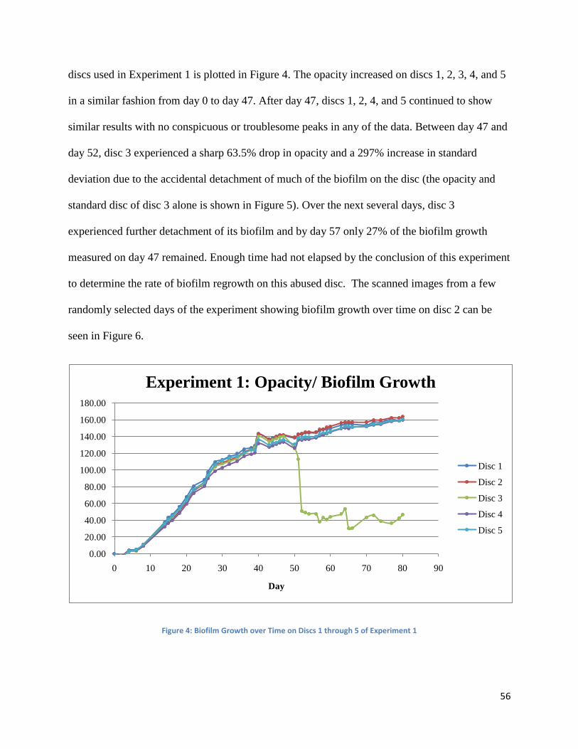
56
discs used in Experiment 1 is plotted in Figure 4. The opacity increased on discs 1, 2, 3, 4, and 5
in a similar fashion from day 0 to day 47. After day 47, discs 1, 2, 4, and 5 continued to show
similar results with no conspicuous or troublesome peaks in any of the data. Between day 47 and
day 52, disc 3 experienced a sharp 63.5% drop in opacity and a 297% increase in standard
deviation due to the accidental detachment of much of the biofilm on the disc (the opacity and
standard disc of disc 3 alone is shown in Figure 5). Over the next several days, disc 3
experienced further detachment of its biofilm and by day 57 only 27% of the biofilm growth
measured on day 47 remained. Enough time had not elapsed by the conclusion of this experiment
to determine the rate of biofilm regrowth on this abused disc. The scanned images from a few
randomly selected days of the experiment showing biofilm growth over time on disc 2 can be
seen in Figure 6.
Figure 4: Biofilm Growth over Time on Discs 1 through 5 of Experiment 1
0.00
20.00
40.00
60.00
80.00
100.00
120.00
140.00
160.00
180.00
0 10 20 30 40 50 60 70 80 90
Day
Experiment 1: Opacity/ Biofilm Growth
Disc 1
Disc 2
Disc 3
Disc 4
Disc 5
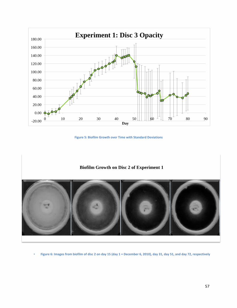
57
Figure 5: Biofilm Growth over Time with Standard Deviations
-20.00
0.00
20.00
40.00
60.00
80.00
100.00
120.00
140.00
160.00
180.00
0 10 20 30 40 50 60 70 80 90
Day
Experiment 1: Disc 3 Opacity
Biofilm Growth on Disc 2 of Experiment 1
• Figure 6: Images from biofilm of disc 2 on day 15 (day 1 = December 6, 2010), day 31, day 51, and day 72, respectively

58
4.1.2 Fluorescence Spectroscopy
The fluorescence absorption peaks for both the substrate and the reactor samples taken
from Experiment 1 remained relatively stable throughout the course of the experiment (see
Figure 7). The intensity of the peak from the reactor samples, and hence the relative protein
concentrations, which are indicative of the bacterial biomass, remained consistantly lower than
those of the substrate samples from day 1 to day 80. The sharp peak in the fluoresce absorption
on day 24 of the substrate sample could be attributed to an array of environmemtal factors, but
does not seem to be evidence of any major change or occurance within the experiment. This data
confirms that the biofilm has indeed matured enough to begin the removal of organic materials
from the wastewater.
The slight decrease which occurs from day 61 to day 63 may be attributed to the addition
of the heavy metal nickel to the Experiment 1 substrate on day 59. Previous studies have
determined that the introduction of the heavy metals Ni+2
or Cu+2
at a concentration of 0.2 mg/L
to the substrate of a reactor can quench the fluorescnce of the wastewater sample by as much as
40%. (Quenching is stabilized at higher concentrations of these metal ions). This occurs due to
the affinity the metal ions possess for certain functional groups directly attached to aromatic
rings, such as those incorporated in tryptophan. The chelation of the metal ions with the aromatic
compounds results in the deactivation of the shared electrons and quenching of the fluorescence.
The mere fact that 0.25 mg/L of nickel was added to the substrate in this experiment would
explain why the fluoresence intensity decreased only a very slight amount. (metal ions and
fluorescence) [47].
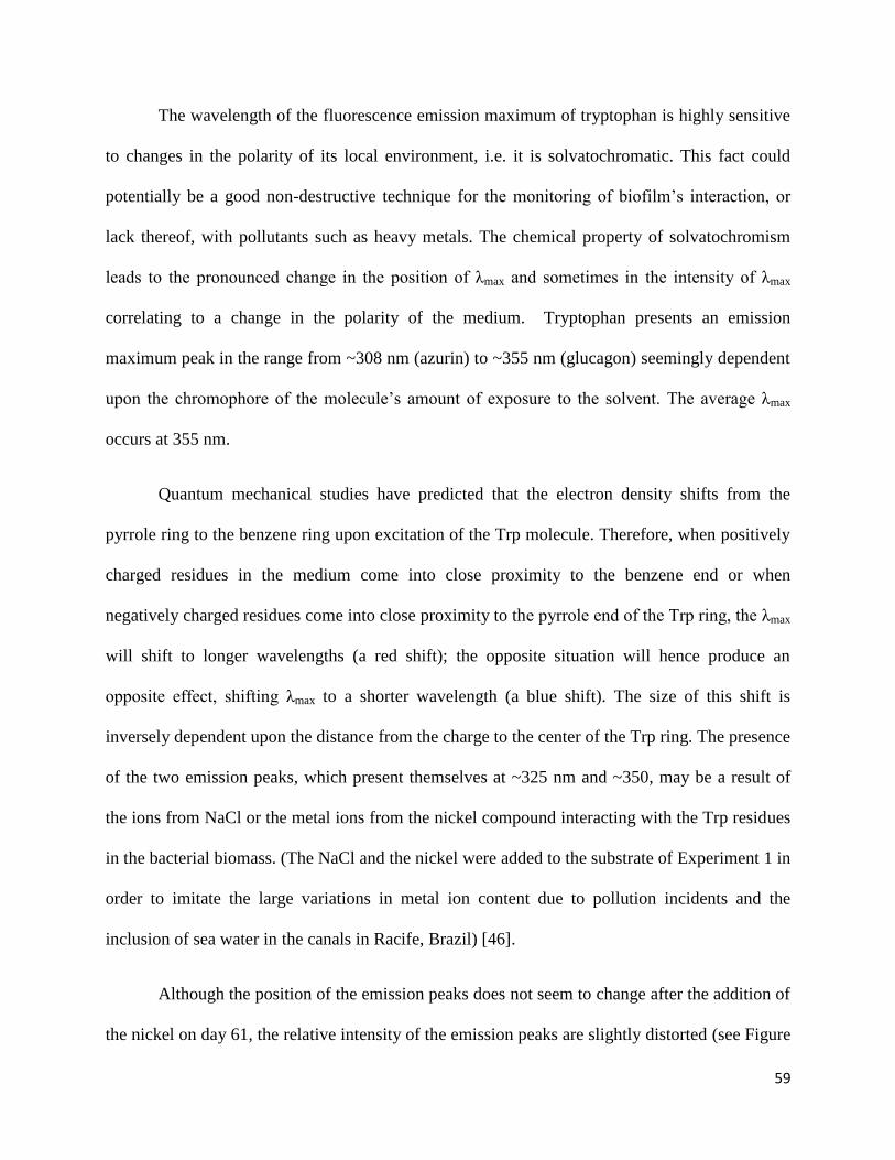
59
The wavelength of the fluorescence emission maximum of tryptophan is highly sensitive
to changes in the polarity of its local environment, i.e. it is solvatochromatic. This fact could
potentially be a good non-destructive technique for the monitoring of biofilm’s interaction, or
lack thereof, with pollutants such as heavy metals. The chemical property of solvatochromism
leads to the pronounced change in the position of λmax and sometimes in the intensity of λmax
correlating to a change in the polarity of the medium. Tryptophan presents an emission
maximum peak in the range from ~308 nm (azurin) to ~355 nm (glucagon) seemingly dependent
upon the chromophore of the molecule’s amount of exposure to the solvent. The average λmax
occurs at 355 nm.
Quantum mechanical studies have predicted that the electron density shifts from the
pyrrole ring to the benzene ring upon excitation of the Trp molecule. Therefore, when positively
charged residues in the medium come into close proximity to the benzene end or when
negatively charged residues come into close proximity to the pyrrole end of the Trp ring, the λmax
will shift to longer wavelengths (a red shift); the opposite situation will hence produce an
opposite effect, shifting λmax to a shorter wavelength (a blue shift). The size of this shift is
inversely dependent upon the distance from the charge to the center of the Trp ring. The presence
of the two emission peaks, which present themselves at ~325 nm and ~350, may be a result of
the ions from NaCl or the metal ions from the nickel compound interacting with the Trp residues
in the bacterial biomass. (The NaCl and the nickel were added to the substrate of Experiment 1 in
order to imitate the large variations in metal ion content due to pollution incidents and the
inclusion of sea water in the canals in Racife, Brazil) [46].
Although the position of the emission peaks does not seem to change after the addition of
the nickel on day 61, the relative intensity of the emission peaks are slightly distorted (see Figure

60
8). The peak located at ~350 nm seems to increase in intensity while the peak located at ~325 nm
seems to decrease in intensity. Then, by day 74 and the conclusion of the experimentation with
the 0.25 mg/L concentration of nickel in the substrate, the peaks have both shifted back to their
original relative intensities (where they were located before nickel was added). It appears that the
biofilm is in some manner interacting with or affected by the nickel in the substrate, but
unfortunately it appears that the conclusion of this experiment occurred too soon to gain any
concrete results in regards to the heavy metal-biofilm interaction. This is important to know for
designing more efficient biofilms or wastewater filtration devices to deal with heavy metal
contamination.
Figure 7: Protein Levels in Water Samples from the Reactor and Substrate of Experiment 1 Over Time
0
100
200
300
400
500
600
700
0 10 20 30 40 50 60 70 80 90
Pro
tein
(A
rbit
rary
Un
its)
Day
Experiment 1: Protein Levels
Reactor
Substrate
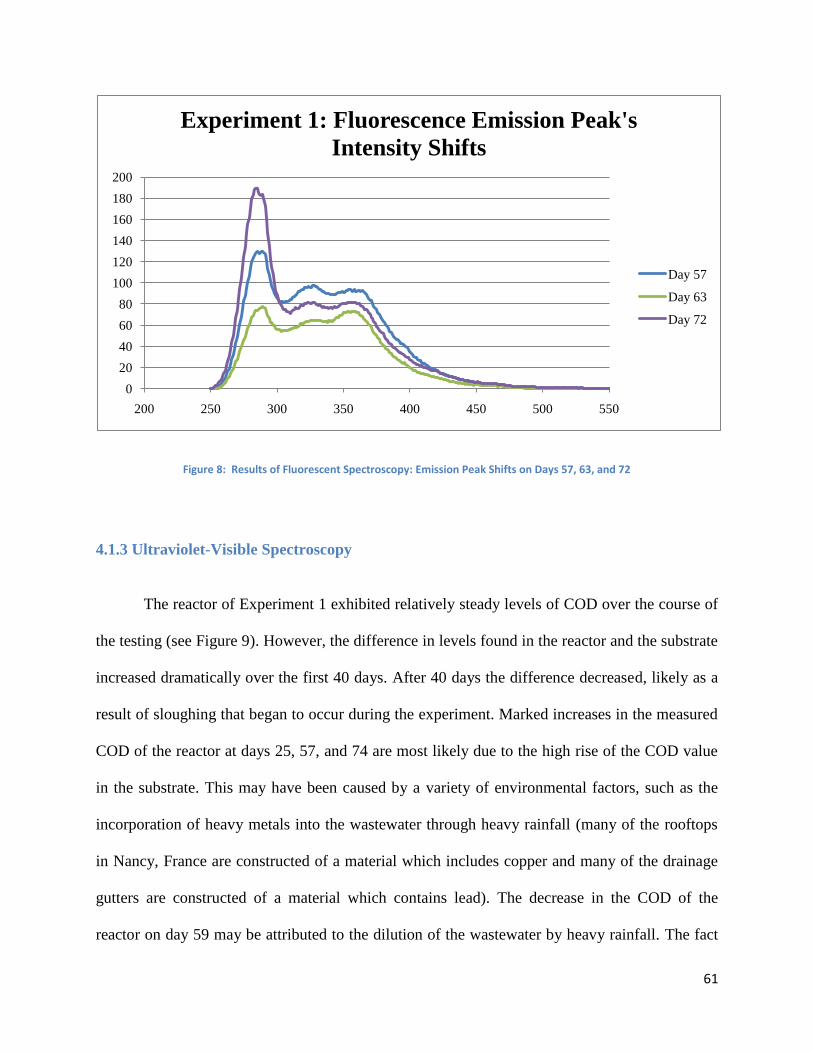
61
Figure 8: Results of Fluorescent Spectroscopy: Emission Peak Shifts on Days 57, 63, and 72
4.1.3 Ultraviolet-Visible Spectroscopy
The reactor of Experiment 1 exhibited relatively steady levels of COD over the course of
the testing (see Figure 9). However, the difference in levels found in the reactor and the substrate
increased dramatically over the first 40 days. After 40 days the difference decreased, likely as a
result of sloughing that began to occur during the experiment. Marked increases in the measured
COD of the reactor at days 25, 57, and 74 are most likely due to the high rise of the COD value
in the substrate. This may have been caused by a variety of environmental factors, such as the
incorporation of heavy metals into the wastewater through heavy rainfall (many of the rooftops
in Nancy, France are constructed of a material which includes copper and many of the drainage
gutters are constructed of a material which contains lead). The decrease in the COD of the
reactor on day 59 may be attributed to the dilution of the wastewater by heavy rainfall. The fact
0
20
40
60
80
100
120
140
160
180
200
200 250 300 350 400 450 500 550
Experiment 1: Fluorescence Emission Peak's
Intensity Shifts
Day 57
Day 63
Day 72
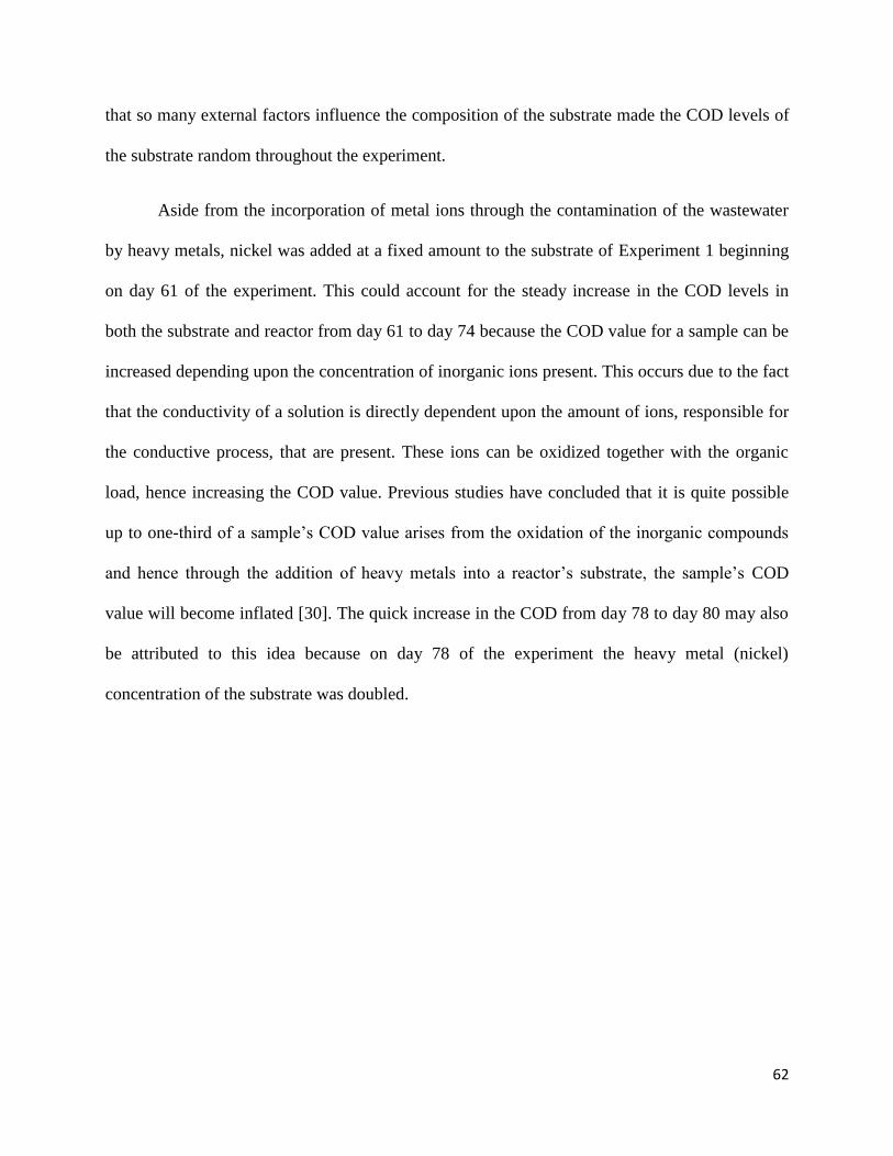
62
that so many external factors influence the composition of the substrate made the COD levels of
the substrate random throughout the experiment.
Aside from the incorporation of metal ions through the contamination of the wastewater
by heavy metals, nickel was added at a fixed amount to the substrate of Experiment 1 beginning
on day 61 of the experiment. This could account for the steady increase in the COD levels in
both the substrate and reactor from day 61 to day 74 because the COD value for a sample can be
increased depending upon the concentration of inorganic ions present. This occurs due to the fact
that the conductivity of a solution is directly dependent upon the amount of ions, responsible for
the conductive process, that are present. These ions can be oxidized together with the organic
load, hence increasing the COD value. Previous studies have concluded that it is quite possible
up to one-third of a sample’s COD value arises from the oxidation of the inorganic compounds
and hence through the addition of heavy metals into a reactor’s substrate, the sample’s COD
value will become inflated [30]. The quick increase in the COD from day 78 to day 80 may also
be attributed to this idea because on day 78 of the experiment the heavy metal (nickel)
concentration of the substrate was doubled.
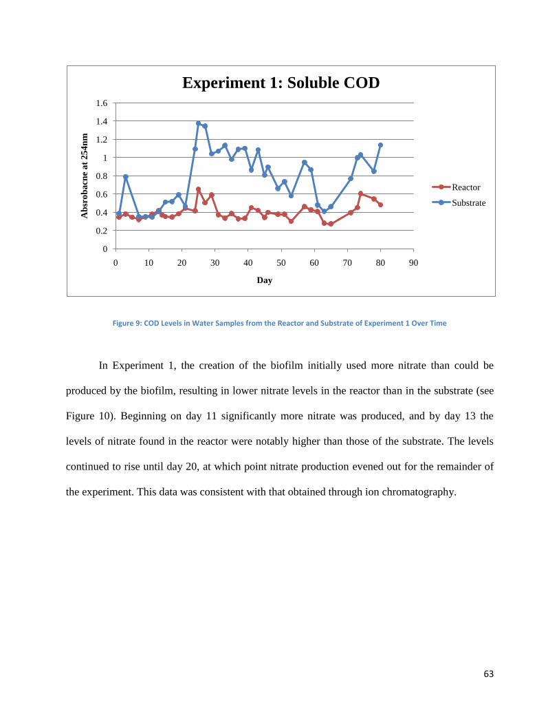
63
Figure 9: COD Levels in Water Samples from the Reactor and Substrate of Experiment 1 Over Time
In Experiment 1, the creation of the biofilm initially used more nitrate than could be
produced by the biofilm, resulting in lower nitrate levels in the reactor than in the substrate (see
Figure 10). Beginning on day 11 significantly more nitrate was produced, and by day 13 the
levels of nitrate found in the reactor were notably higher than those of the substrate. The levels
continued to rise until day 20, at which point nitrate production evened out for the remainder of
the experiment. This data was consistent with that obtained through ion chromatography.
0
0.2
0.4
0.6
0.8
1
1.2
1.4
1.6
0 10 20 30 40 50 60 70 80 90
Ab
sro
ba
cne
at
25
4n
m
Day
Experiment 1: Soluble COD
Reactor
Substrate

64
Figure 10: Nitrate Production in Water Samples from the Reactor and Substrate of Experiment 1 Over Time
4.1.4 Ion Chromatography and the Ammonium Test
The ammonia, nitrate, and nitrite levels within the rotating biological reactor Experiment
1 were collected through the analytical techniques of Ion Chromatography and the Ammonium
Test. The values obtained in these tests were then all transformed (from mg NO2/L, for example)
into the same units (mg Nitrogen/L) and compiled into the graph shown in Figure 11. This graph
begins on day 43 because the ion chromatography results were not collected prior to this date.
The levels of ammonia exhibit a downward trend as time progresses and as the biofilm
develops (ammonium results are isolated and are shown over a longer period of time in Figure
13). This is as expected because as the biofilm grows, it is accumulating more and more
nitrifying bacteria. These bacteria then convert the ammonia into the end product of nitrate in
order to perform their necessary life functions. In accordance to this idea, the overall decreasing
levels of ammonia coincide with a rise in nitrite levels beginning at or before day 43 (because the
0.0000
0.5000
1.0000
1.5000
2.0000
2.5000
3.0000
3.5000
0 10 20 30 40 50 60 70 80 90
[NO
3]
mg
/L
Day
Experiment 1: Nitrate Production (UV-Vis)
Substrate
Reactor
65
graph does not include any data from before this time point, the exact date that this increase
began cannot be known). The maximum level of nitrite and the minimum level of nitrate are
observed on day 59. Subsequent to this date, the nitrite levels slowly begin to decline as the
nitrate levels slowly begin to increase. At about day 71, the nitrate levels begin to plateau, while
the nitrite levels begin to return to their original levels. The nitrate levels are significantly lower
than the nitrite levels. It is possible that the addition of salt to the substrate interfered with the
nitrification process. The sodium ions from the sodium chloride may have formed molecules
with the oxygen, such as sodium oxide or sodium peroxide, thereby decreasing the oxygen
levels, which are required to convert nitrite to nitrate. Overall, although the nitrite levels rose and
fell dramatically throughout the experiment, the concentration of nitrite at the beginning of the
experiment and at the end of the experiment remained about equal. This occurs because of the
role which nitrite plays in the nitrification pathway, which is that of an intermediate between the
ammonia and the nitrate. The nitrite and nitrate levels are magnified for easier viewing in Figure
12.
All these results are to be expected of the bacteria in the biofilm, because the nitrification
process began when the biofilm was mature enough to undergo this endeavor. These results are
further supported by those obtained for the nitrate production from UV-Visible Spectroscopy.
However, it is quite interesting that the nitrification process appears to have started (on day 59)
at the same exact time that the heavy metal nickel was introduced to the substrate, perhaps
indicating that the introduction of these metal ions into the substrate may have somehow
stimulated the nitrification process. This idea could not be confirmed because the experiment
was not maintained long enough after the addition of nickel to yield any substantiating results.
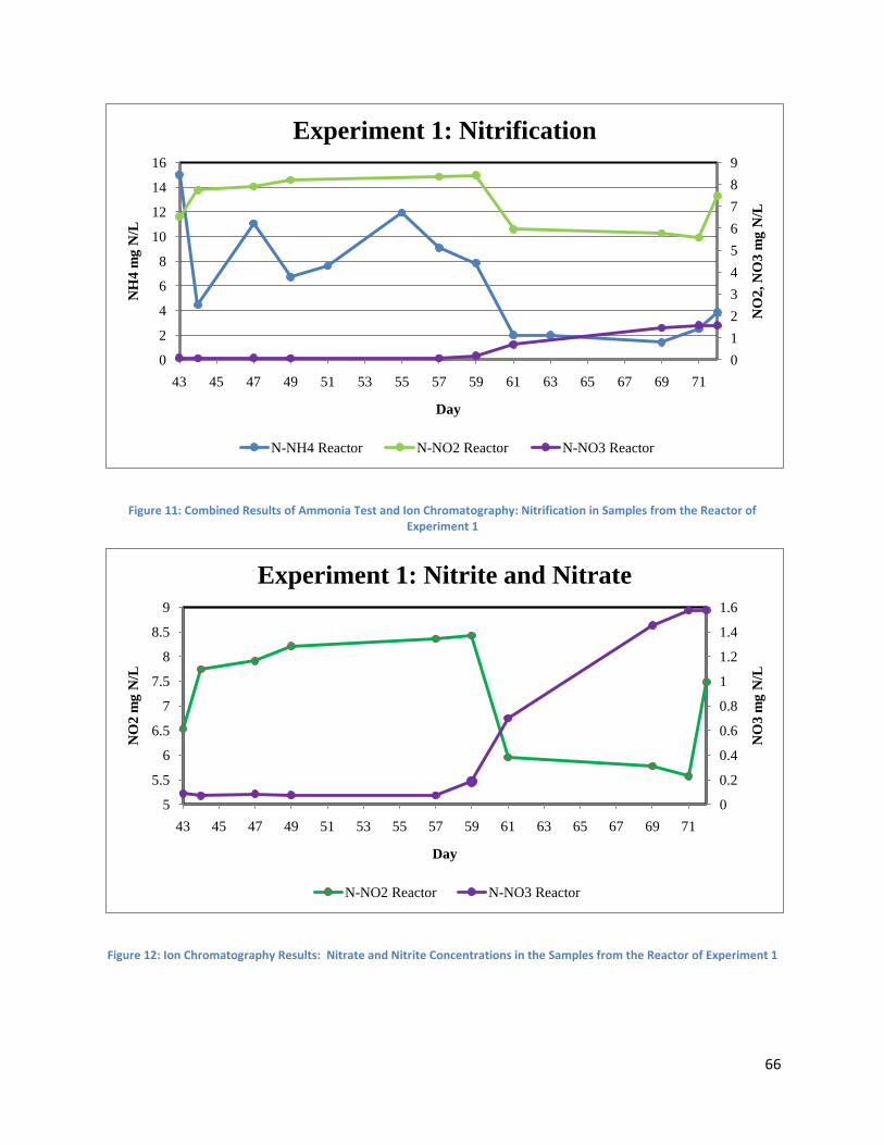
66
Figure 11: Combined Results of Ammonia Test and Ion Chromatography: Nitrification in Samples from the Reactor of Experiment 1
Figure 12: Ion Chromatography Results: Nitrate and Nitrite Concentrations in the Samples from the Reactor of Experiment 1
0
1
2
3
4
5
6
7
8
9
0
2
4
6
8
10
12
14
16
43 45 47 49 51 53 55 57 59 61 63 65 67 69 71
NO
2, N
O3
mg
N/L
NH
4 m
g N
/L
Day
Experiment 1: Nitrification
N-NH4 Reactor N-NO2 Reactor N-NO3 Reactor
0
0.2
0.4
0.6
0.8
1
1.2
1.4
1.6
5
5.5
6
6.5
7
7.5
8
8.5
9
43 45 47 49 51 53 55 57 59 61 63 65 67 69 71
NO
3 m
g N
/L
NO
2 m
g N
/L
Day
Experiment 1: Nitrite and Nitrate
N-NO2 Reactor N-NO3 Reactor
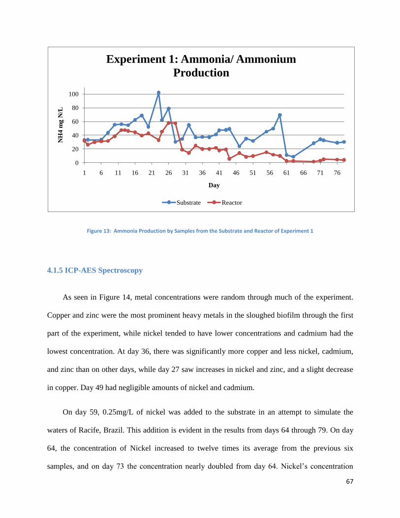
67
Figure 13: Ammonia Production by Samples from the Substrate and Reactor of Experiment 1
4.1.5 ICP-AES Spectroscopy
As seen in Figure 14, metal concentrations were random through much of the experiment.
Copper and zinc were the most prominent heavy metals in the sloughed biofilm through the first
part of the experiment, while nickel tended to have lower concentrations and cadmium had the
lowest concentration. At day 36, there was significantly more copper and less nickel, cadmium,
and zinc than on other days, while day 27 saw increases in nickel and zinc, and a slight decrease
in copper. Day 49 had negligible amounts of nickel and cadmium.
On day 59, 0.25mg/L of nickel was added to the substrate in an attempt to simulate the
waters of Racife, Brazil. This addition is evident in the results from days 64 through 79. On day
64, the concentration of Nickel increased to twelve times its average from the previous six
samples, and on day 73 the concentration nearly doubled from day 64. Nickel’s concentration
0
20
40
60
80
100
1 6 11 16 21 26 31 36 41 46 51 56 61 66 71 76
NH
4 m
g N
/L
Day
Experiment 1: Ammonia/ Ammonium
Production
Substrate Reactor
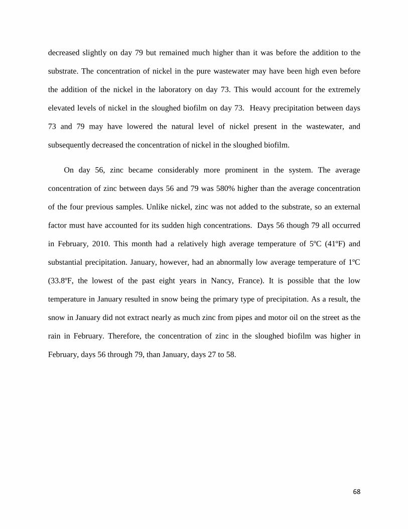
68
decreased slightly on day 79 but remained much higher than it was before the addition to the
substrate. The concentration of nickel in the pure wastewater may have been high even before
the addition of the nickel in the laboratory on day 73. This would account for the extremely
elevated levels of nickel in the sloughed biofilm on day 73. Heavy precipitation between days
73 and 79 may have lowered the natural level of nickel present in the wastewater, and
subsequently decreased the concentration of nickel in the sloughed biofilm.
On day 56, zinc became considerably more prominent in the system. The average
concentration of zinc between days 56 and 79 was 580% higher than the average concentration
of the four previous samples. Unlike nickel, zinc was not added to the substrate, so an external
factor must have accounted for its sudden high concentrations. Days 56 though 79 all occurred
in February, 2010. This month had a relatively high average temperature of 5ºC (41ºF) and
substantial precipitation. January, however, had an abnormally low average temperature of 1ºC
(33.8ºF, the lowest of the past eight years in Nancy, France). It is possible that the low
temperature in January resulted in snow being the primary type of precipitation. As a result, the
snow in January did not extract nearly as much zinc from pipes and motor oil on the street as the
rain in February. Therefore, the concentration of zinc in the sloughed biofilm was higher in
February, days 56 through 79, than January, days 27 to 58.
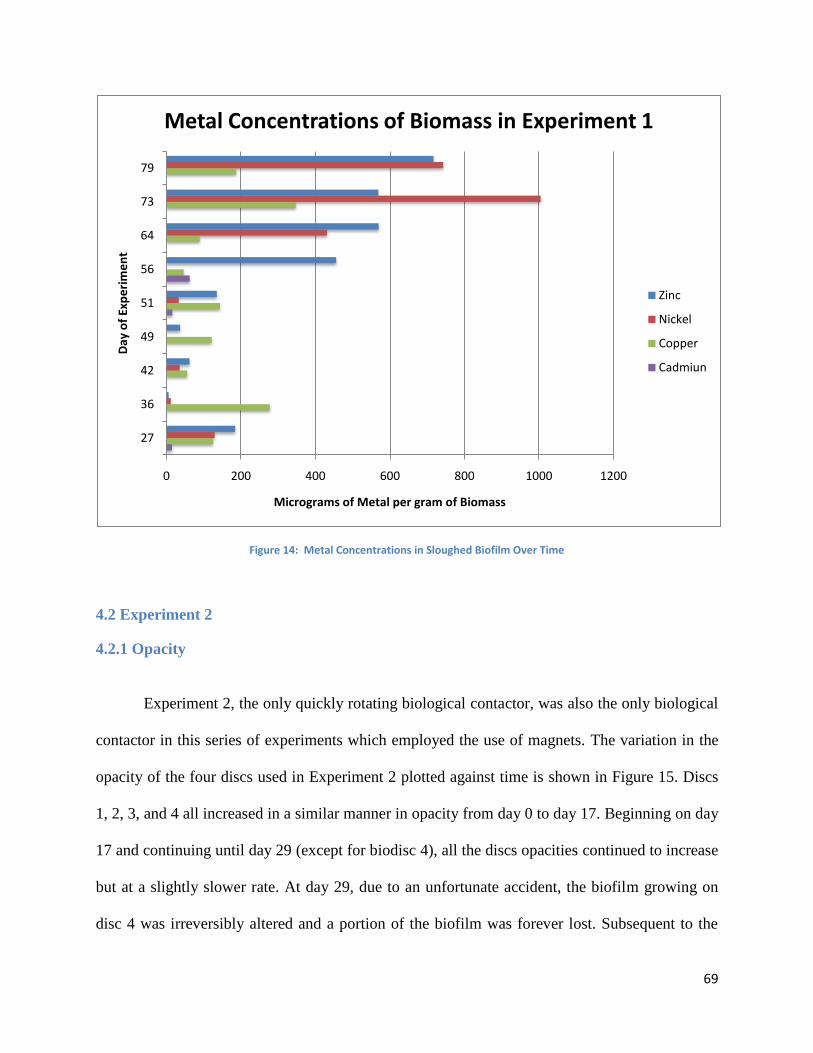
69
Figure 14: Metal Concentrations in Sloughed Biofilm Over Time
4.2 Experiment 2
4.2.1 Opacity
Experiment 2, the only quickly rotating biological contactor, was also the only biological
contactor in this series of experiments which employed the use of magnets. The variation in the
opacity of the four discs used in Experiment 2 plotted against time is shown in Figure 15. Discs
1, 2, 3, and 4 all increased in a similar manner in opacity from day 0 to day 17. Beginning on day
17 and continuing until day 29 (except for biodisc 4), all the discs opacities continued to increase
but at a slightly slower rate. At day 29, due to an unfortunate accident, the biofilm growing on
disc 4 was irreversibly altered and a portion of the biofilm was forever lost. Subsequent to the
0 200 400 600 800 1000 1200
27
36
42
49
51
56
64
73
79
Micrograms of Metal per gram of Biomass
Day
of
Exp
eri
me
nt
Metal Concentrations of Biomass in Experiment 1
Zinc
Nickel
Copper
Cadmiun
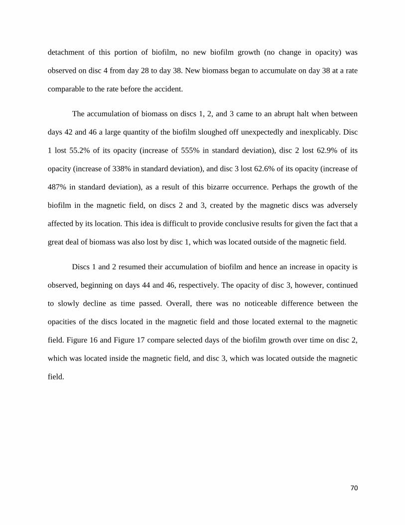
70
detachment of this portion of biofilm, no new biofilm growth (no change in opacity) was
observed on disc 4 from day 28 to day 38. New biomass began to accumulate on day 38 at a rate
comparable to the rate before the accident.
The accumulation of biomass on discs 1, 2, and 3 came to an abrupt halt when between
days 42 and 46 a large quantity of the biofilm sloughed off unexpectedly and inexplicably. Disc
1 lost 55.2% of its opacity (increase of 555% in standard deviation), disc 2 lost 62.9% of its
opacity (increase of 338% in standard deviation), and disc 3 lost 62.6% of its opacity (increase of
487% in standard deviation), as a result of this bizarre occurrence. Perhaps the growth of the
biofilm in the magnetic field, on discs 2 and 3, created by the magnetic discs was adversely
affected by its location. This idea is difficult to provide conclusive results for given the fact that a
great deal of biomass was also lost by disc 1, which was located outside of the magnetic field.
Discs 1 and 2 resumed their accumulation of biofilm and hence an increase in opacity is
observed, beginning on days 44 and 46, respectively. The opacity of disc 3, however, continued
to slowly decline as time passed. Overall, there was no noticeable difference between the
opacities of the discs located in the magnetic field and those located external to the magnetic
field. Figure 16 and Figure 17 compare selected days of the biofilm growth over time on disc 2,
which was located inside the magnetic field, and disc 3, which was located outside the magnetic
field.
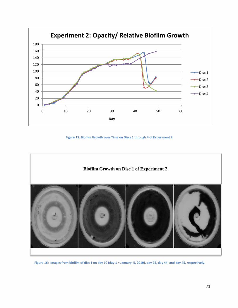
71
Figure 15: Biofilm Growth over Time on Discs 1 through 4 of Experiment 2
Figure 16: Images from biofilm of disc 1 on day 10 (day 1 = January, 5, 2010), day 25, day 44, and day 45, respectively.
0
20
40
60
80
100
120
140
160
180
0 10 20 30 40 50 60
Day
Experiment 2: Opacity/ Relative Biofilm Growth
Disc 1
Disc 2
Disc 3
Disc 4
Biofilm Growth on Disc 1 of Experiment 2.

72
Figure 17: Images from biofilm of disc 3 on day 10 (day 1 = January, 5, 2010), day 25, day 44, and day 45, respectively.
4.2.2 Fluorescence Spectroscopy
As seen in Figure 18, the samples from the reactor of Experiment 2 consistently had a
lower amount of protein than the samples from the substrate. The biofilm absorbs and removes
organic material from the wastewater in the reactor and converts the organic nitrogen to an end
product of nitrate, subsequently lowering the amount of trypophan in the reactor. Therefore, as
expected, less protein and residual organic matter were present in the samples from the reactor
than from the substrate each day [42]. In addition, the results showed that the biofilm more
efficiently removed protein from the wastewater in the reactor as time progressed. As the biofilm
grew thicker, more ammonium was converted to nitrite and then oxidized to nitrate resulting in
lower concentrations of fluorecing tryptophan, which can be used to monitor biofilm efficiency.
Biofilm Growth on Disc 3 of Experiment 2

73
Figure 18: Protein Levels in Samples from the Reactor and Substrate of Experiment 2
4.2.3 Ultraviolet-Visible Spectroscopy
The levels of COD in the reactor of Experiment 2 were generally lower than those found
in the substrate, with a negative trend over time as the biofilm thickness and effectiveness
increased (see Figure 19). As expected, the levels found in the substrate were random. Near the
beginning of week 2 of the experiment, a large spike in COD levels occurred within the reactor,
which is unexplained.
0
50
100
150
200
250
300
350
400
450
500
0 10 20 30 40 50 60
Days
Experiment 2: Protein Levels
Reactor
Substrate
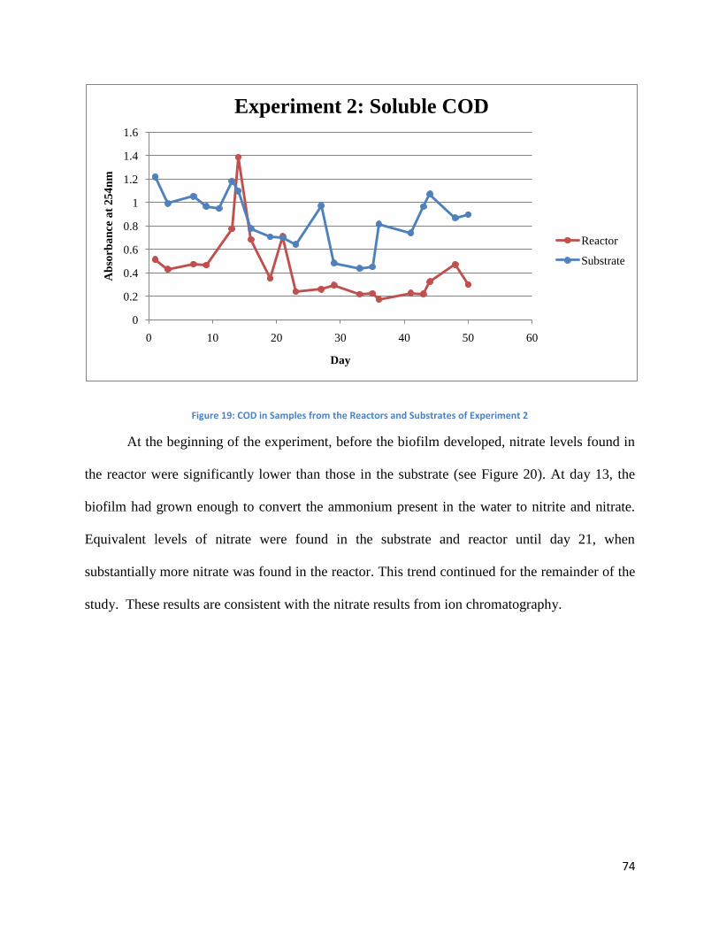
74
Figure 19: COD in Samples from the Reactors and Substrates of Experiment 2
At the beginning of the experiment, before the biofilm developed, nitrate levels found in
the reactor were significantly lower than those in the substrate (see Figure 20). At day 13, the
biofilm had grown enough to convert the ammonium present in the water to nitrite and nitrate.
Equivalent levels of nitrate were found in the substrate and reactor until day 21, when
substantially more nitrate was found in the reactor. This trend continued for the remainder of the
study. These results are consistent with the nitrate results from ion chromatography.
0
0.2
0.4
0.6
0.8
1
1.2
1.4
1.6
0 10 20 30 40 50 60
Ab
sorb
an
ce a
t 2
54
nm
Day
Experiment 2: Soluble COD
Reactor
Substrate
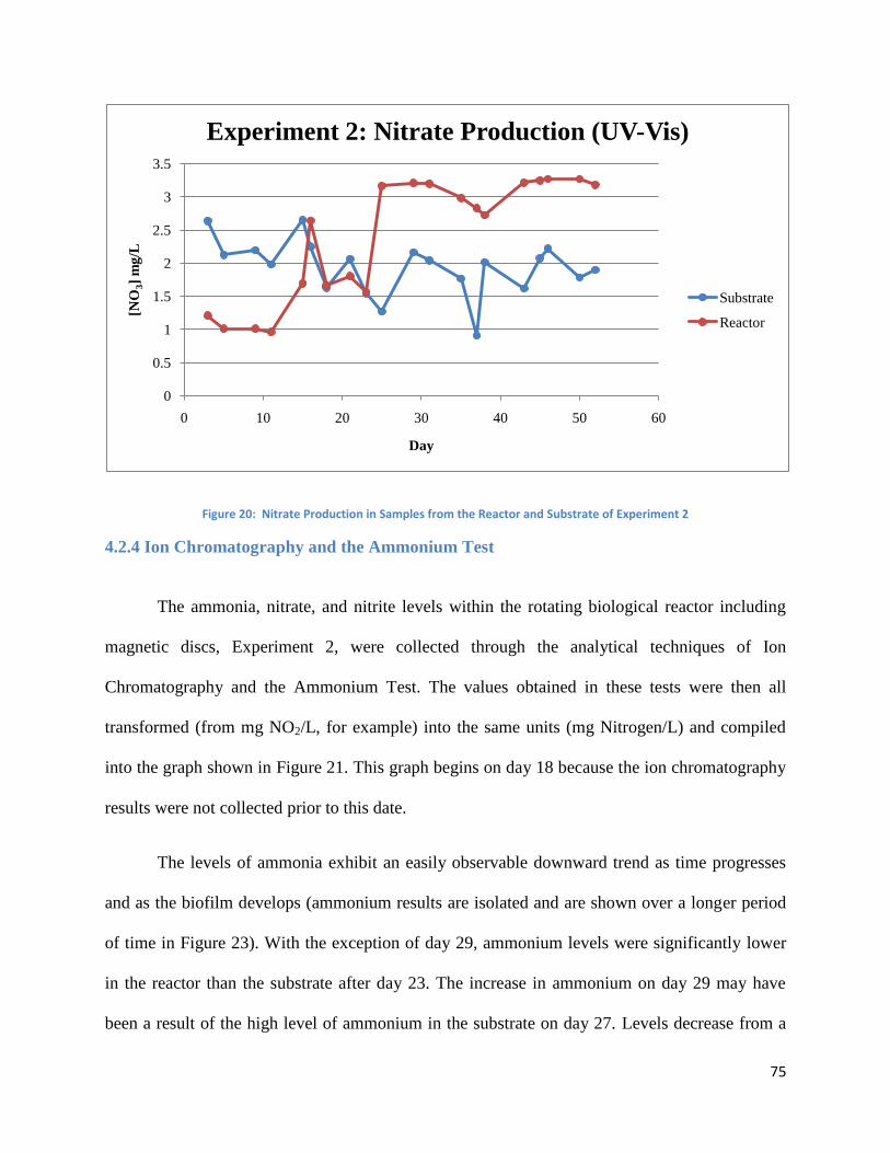
75
Figure 20: Nitrate Production in Samples from the Reactor and Substrate of Experiment 2
4.2.4 Ion Chromatography and the Ammonium Test
The ammonia, nitrate, and nitrite levels within the rotating biological reactor including
magnetic discs, Experiment 2, were collected through the analytical techniques of Ion
Chromatography and the Ammonium Test. The values obtained in these tests were then all
transformed (from mg NO2/L, for example) into the same units (mg Nitrogen/L) and compiled
into the graph shown in Figure 21. This graph begins on day 18 because the ion chromatography
results were not collected prior to this date.
The levels of ammonia exhibit an easily observable downward trend as time progresses
and as the biofilm develops (ammonium results are isolated and are shown over a longer period
of time in Figure 23). With the exception of day 29, ammonium levels were significantly lower
in the reactor than the substrate after day 23. The increase in ammonium on day 29 may have
been a result of the high level of ammonium in the substrate on day 27. Levels decrease from a
0
0.5
1
1.5
2
2.5
3
3.5
0 10 20 30 40 50 60
[NO
3]
mg
/L
Day
Experiment 2: Nitrate Production (UV-Vis)
Substrate
Reactor
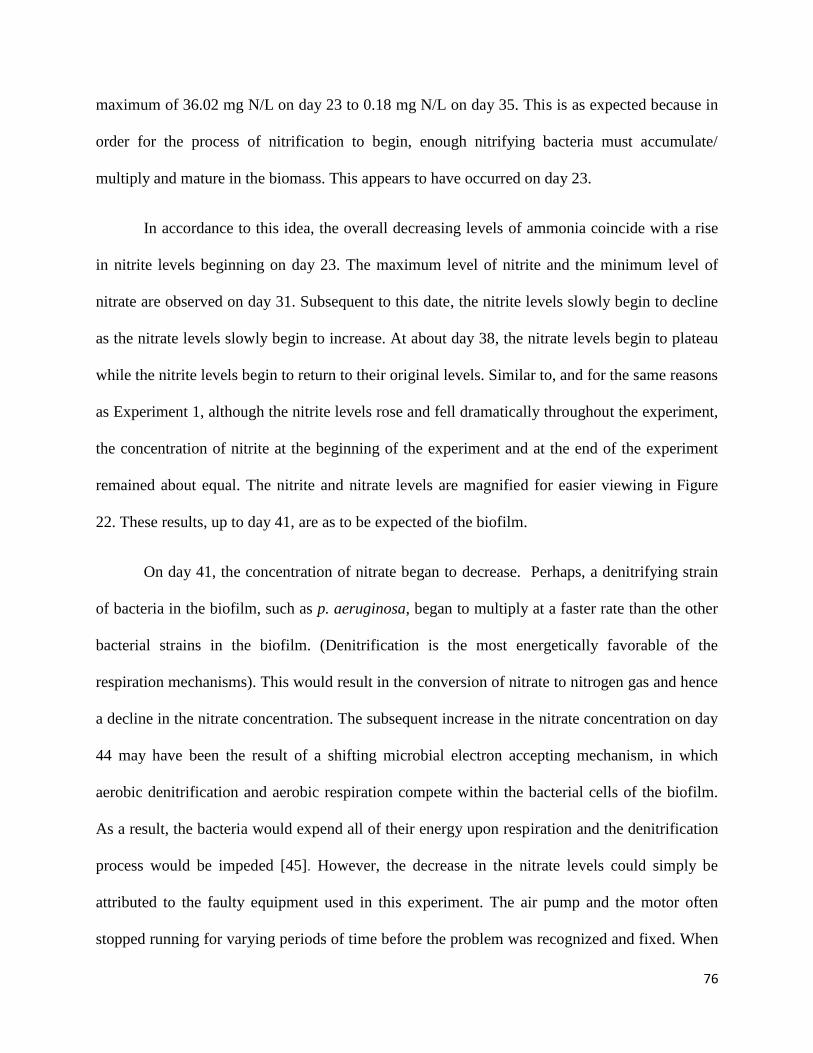
76
maximum of 36.02 mg N/L on day 23 to 0.18 mg N/L on day 35. This is as expected because in
order for the process of nitrification to begin, enough nitrifying bacteria must accumulate/
multiply and mature in the biomass. This appears to have occurred on day 23.
In accordance to this idea, the overall decreasing levels of ammonia coincide with a rise
in nitrite levels beginning on day 23. The maximum level of nitrite and the minimum level of
nitrate are observed on day 31. Subsequent to this date, the nitrite levels slowly begin to decline
as the nitrate levels slowly begin to increase. At about day 38, the nitrate levels begin to plateau
while the nitrite levels begin to return to their original levels. Similar to, and for the same reasons
as Experiment 1, although the nitrite levels rose and fell dramatically throughout the experiment,
the concentration of nitrite at the beginning of the experiment and at the end of the experiment
remained about equal. The nitrite and nitrate levels are magnified for easier viewing in Figure
22. These results, up to day 41, are as to be expected of the biofilm.
On day 41, the concentration of nitrate began to decrease. Perhaps, a denitrifying strain
of bacteria in the biofilm, such as p. aeruginosa, began to multiply at a faster rate than the other
bacterial strains in the biofilm. (Denitrification is the most energetically favorable of the
respiration mechanisms). This would result in the conversion of nitrate to nitrogen gas and hence
a decline in the nitrate concentration. The subsequent increase in the nitrate concentration on day
44 may have been the result of a shifting microbial electron accepting mechanism, in which
aerobic denitrification and aerobic respiration compete within the bacterial cells of the biofilm.
As a result, the bacteria would expend all of their energy upon respiration and the denitrification
process would be impeded [45]. However, the decrease in the nitrate levels could simply be
attributed to the faulty equipment used in this experiment. The air pump and the motor often
stopped running for varying periods of time before the problem was recognized and fixed. When
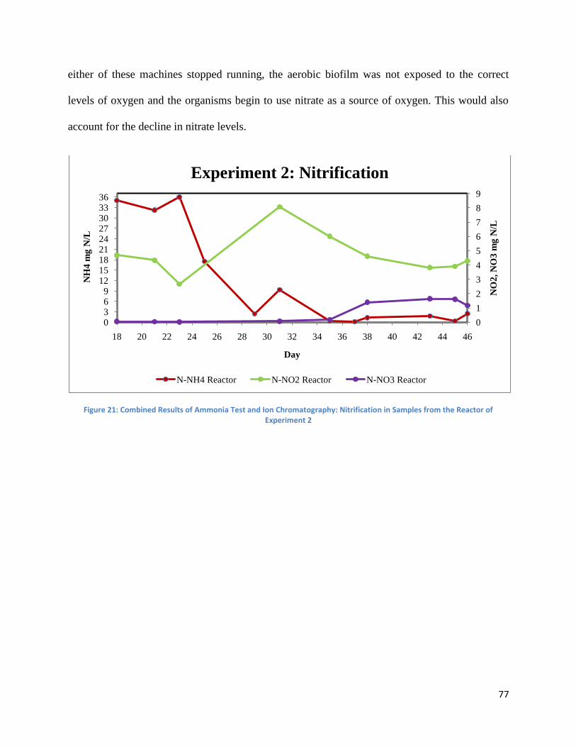
77
either of these machines stopped running, the aerobic biofilm was not exposed to the correct
levels of oxygen and the organisms begin to use nitrate as a source of oxygen. This would also
account for the decline in nitrate levels.
Figure 21: Combined Results of Ammonia Test and Ion Chromatography: Nitrification in Samples from the Reactor of Experiment 2
0
1
2
3
4
5
6
7
8
9
0369
121518212427303336
18 20 22 24 26 28 30 32 34 36 38 40 42 44 46
NO
2, N
O3
mg
N/L
NH
4 m
g N
/L
Day
Experiment 2: Nitrification
N-NH4 Reactor N-NO2 Reactor N-NO3 Reactor
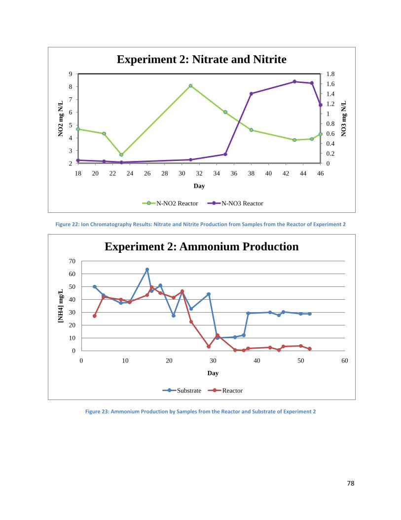
78
Figure 22: Ion Chromatography Results: Nitrate and Nitrite Production from Samples from the Reactor of Experiment 2
Figure 23: Ammonium Production by Samples from the Reactor and Substrate of Experiment 2
0
0.2
0.4
0.6
0.8
1
1.2
1.4
1.6
1.8
2
3
4
5
6
7
8
9
18 20 22 24 26 28 30 32 34 36 38 40 42 44 46
NO
3 m
g N
/L
NO
2 m
g N
/L
Day
Experiment 2: Nitrate and Nitrite
N-NO2 Reactor N-NO3 Reactor
0
10
20
30
40
50
60
70
0 10 20 30 40 50 60
[NH
4]
mg
/L
Day
Experiment 2: Ammonium Production
Substrate Reactor
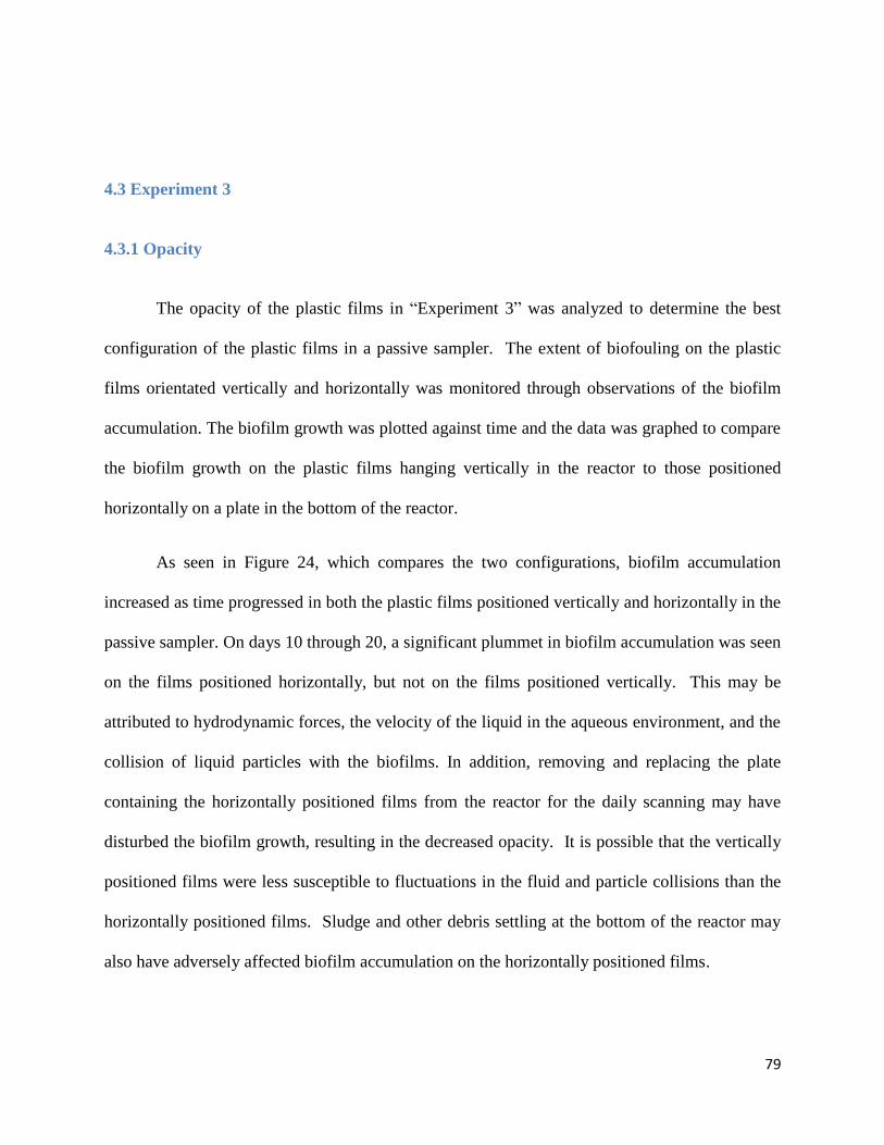
79
4.3 Experiment 3
4.3.1 Opacity
The opacity of the plastic films in “Experiment 3” was analyzed to determine the best
configuration of the plastic films in a passive sampler. The extent of biofouling on the plastic
films orientated vertically and horizontally was monitored through observations of the biofilm
accumulation. The biofilm growth was plotted against time and the data was graphed to compare
the biofilm growth on the plastic films hanging vertically in the reactor to those positioned
horizontally on a plate in the bottom of the reactor.
As seen in Figure 24, which compares the two configurations, biofilm accumulation
increased as time progressed in both the plastic films positioned vertically and horizontally in the
passive sampler. On days 10 through 20, a significant plummet in biofilm accumulation was seen
on the films positioned horizontally, but not on the films positioned vertically. This may be
attributed to hydrodynamic forces, the velocity of the liquid in the aqueous environment, and the
collision of liquid particles with the biofilms. In addition, removing and replacing the plate
containing the horizontally positioned films from the reactor for the daily scanning may have
disturbed the biofilm growth, resulting in the decreased opacity. It is possible that the vertically
positioned films were less susceptible to fluctuations in the fluid and particle collisions than the
horizontally positioned films. Sludge and other debris settling at the bottom of the reactor may
also have adversely affected biofilm accumulation on the horizontally positioned films.
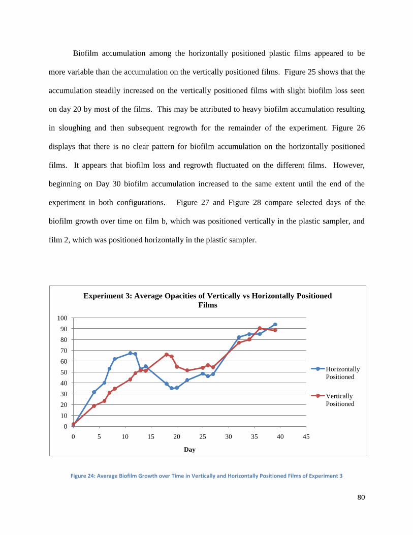
80
Biofilm accumulation among the horizontally positioned plastic films appeared to be
more variable than the accumulation on the vertically positioned films. Figure 25 shows that the
accumulation steadily increased on the vertically positioned films with slight biofilm loss seen
on day 20 by most of the films. This may be attributed to heavy biofilm accumulation resulting
in sloughing and then subsequent regrowth for the remainder of the experiment. Figure 26
displays that there is no clear pattern for biofilm accumulation on the horizontally positioned
films. It appears that biofilm loss and regrowth fluctuated on the different films. However,
beginning on Day 30 biofilm accumulation increased to the same extent until the end of the
experiment in both configurations. Figure 27 and Figure 28 compare selected days of the
biofilm growth over time on film b, which was positioned vertically in the plastic sampler, and
film 2, which was positioned horizontally in the plastic sampler.
Figure 24: Average Biofilm Growth over Time in Vertically and Horizontally Positioned Films of Experiment 3
0
10
20
30
40
50
60
70
80
90
100
0 5 10 15 20 25 30 35 40 45
Day
Experiment 3: Average Opacities of Vertically vs Horizontally Positioned
Films
Horizontally
Positioned
Vertically
Positioned
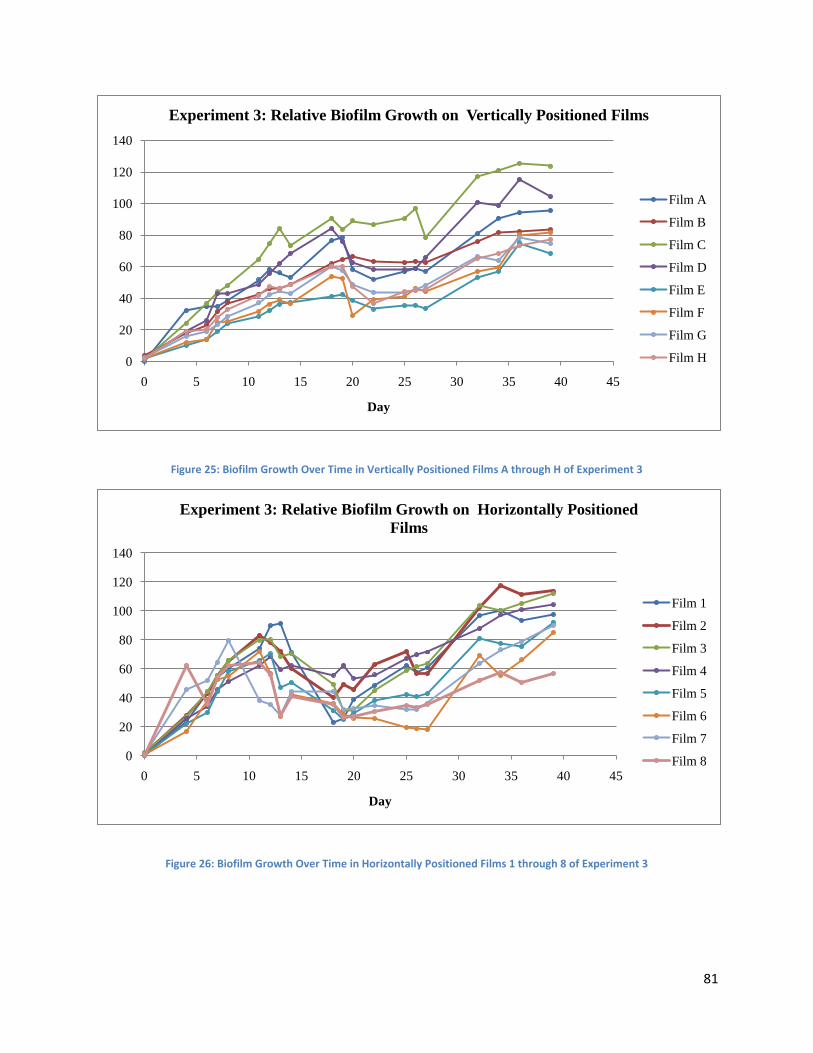
81
Figure 25: Biofilm Growth Over Time in Vertically Positioned Films A through H of Experiment 3
Figure 26: Biofilm Growth Over Time in Horizontally Positioned Films 1 through 8 of Experiment 3
0
20
40
60
80
100
120
140
0 5 10 15 20 25 30 35 40 45
Day
Experiment 3: Relative Biofilm Growth on Vertically Positioned Films
Film A
Film B
Film C
Film D
Film E
Film F
Film G
Film H
0
20
40
60
80
100
120
140
0 5 10 15 20 25 30 35 40 45
Day
Experiment 3: Relative Biofilm Growth on Horizontally Positioned
Films
Film 1
Film 2
Film 3
Film 4
Film 5
Film 6
Film 7
Film 8

82
Figure 27: Images from biofilm of plastic film b on day 1, day 7, day 14, day 20, day 25, and day 34.
Biofilm growth on vertically positioned plastic film b
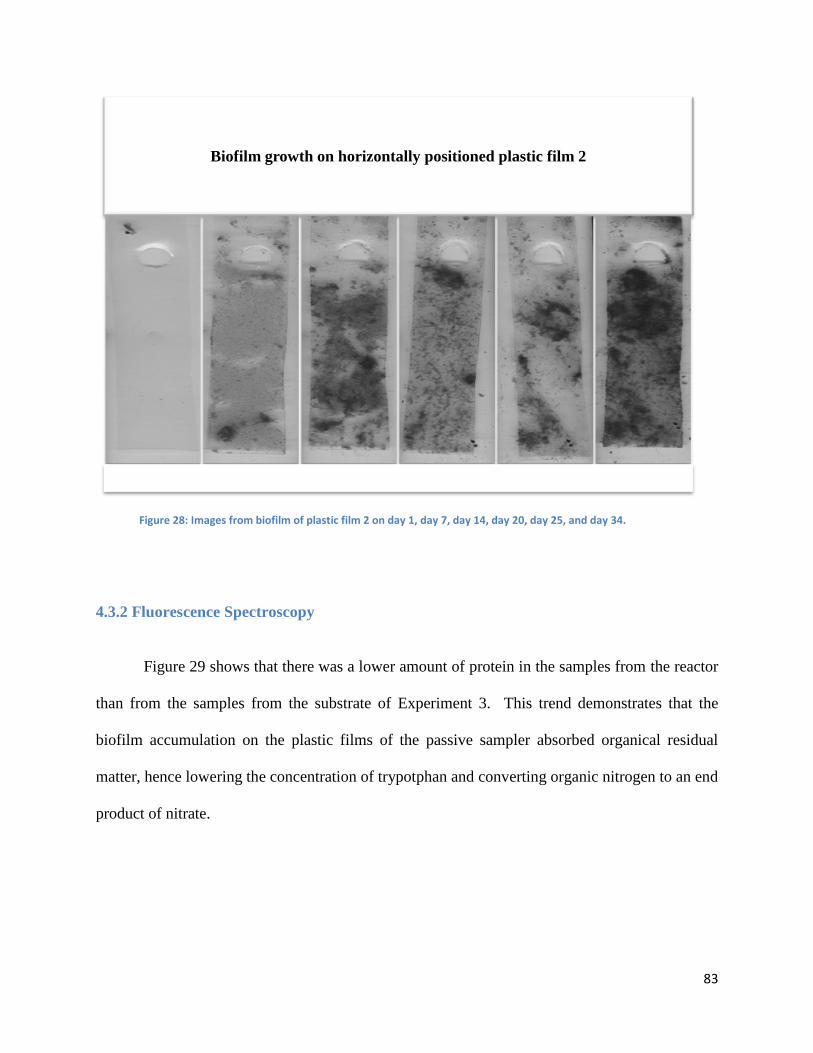
83
Figure 28: Images from biofilm of plastic film 2 on day 1, day 7, day 14, day 20, day 25, and day 34.
4.3.2 Fluorescence Spectroscopy
Figure 29 shows that there was a lower amount of protein in the samples from the reactor
than from the samples from the substrate of Experiment 3. This trend demonstrates that the
biofilm accumulation on the plastic films of the passive sampler absorbed organical residual
matter, hence lowering the concentration of trypotphan and converting organic nitrogen to an end
product of nitrate.
Biofilm growth on horizontally positioned plastic film 2

84
Figure 29: Protein Levels from Samples from the Reactor and Substrate of Experiment 3
4.3.3 Ultraviolet-Visible Spectroscopy
The COD levels found in the reactor of Experiment 3 through UV-Visible Spectroscopy,
seen in Figure 30, were lower than those found in the substrate. There is also a negative trend
over time, although less pronounced. At days 17 and 33, the measured COD increases, but both
of these increases may be attributed to simultaneous rises in the COD levels of the substrate
being used by the reactor. The levels found in the substrate are random.
0
50
100
150
200
250
300
350
400
450
0 5 10 15 20 25 30 35 40
Days
Experiment 3: Protein Levels
Reactor
Substrate
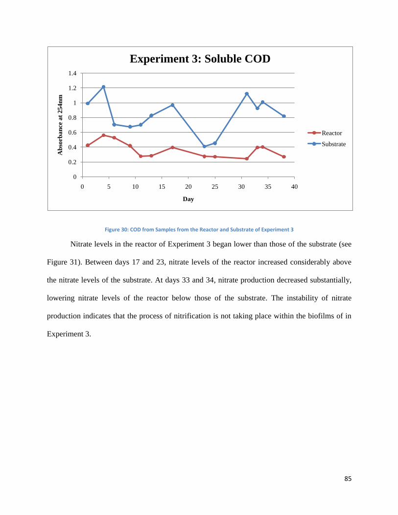
85
Figure 30: COD from Samples from the Reactor and Substrate of Experiment 3
Nitrate levels in the reactor of Experiment 3 began lower than those of the substrate (see
Figure 31). Between days 17 and 23, nitrate levels of the reactor increased considerably above
the nitrate levels of the substrate. At days 33 and 34, nitrate production decreased substantially,
lowering nitrate levels of the reactor below those of the substrate. The instability of nitrate
production indicates that the process of nitrification is not taking place within the biofilms of in
Experiment 3.
0
0.2
0.4
0.6
0.8
1
1.2
1.4
0 5 10 15 20 25 30 35 40
Ab
sorb
an
ce a
t 2
54
nm
Day
Experiment 3: Soluble COD
Reactor
Substrate
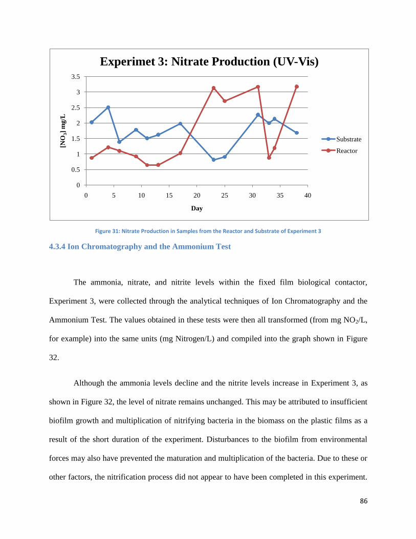
86
Figure 31: Nitrate Production in Samples from the Reactor and Substrate of Experiment 3
4.3.4 Ion Chromatography and the Ammonium Test
The ammonia, nitrate, and nitrite levels within the fixed film biological contactor,
Experiment 3, were collected through the analytical techniques of Ion Chromatography and the
Ammonium Test. The values obtained in these tests were then all transformed (from mg NO2/L,
for example) into the same units (mg Nitrogen/L) and compiled into the graph shown in Figure
32.
Although the ammonia levels decline and the nitrite levels increase in Experiment 3, as
shown in Figure 32, the level of nitrate remains unchanged. This may be attributed to insufficient
biofilm growth and multiplication of nitrifying bacteria in the biomass on the plastic films as a
result of the short duration of the experiment. Disturbances to the biofilm from environmental
forces may also have prevented the maturation and multiplication of the bacteria. Due to these or
other factors, the nitrification process did not appear to have been completed in this experiment.
0
0.5
1
1.5
2
2.5
3
3.5
0 5 10 15 20 25 30 35 40
[NO
3]
mg
/L
Day
Experimet 3: Nitrate Production (UV-Vis)
Substrate
Reactor

87
Figure 33 shows that the levels of ammonia were declining, so it can be surmised that if the
experiment had been allowed to run for an extended period of time, the nitrate levels would have
increased as the other steps of the process transpired.
Figure 32: Combined Results of Ammonia Test and Ion Chromatography: Nitrification in Samples from the Reactor of Experiment 3
0
1
2
3
4
5
6
0
4
8
12
16
20
24
28
32
36
40
6 8 10 12 14 16 18 20 22 24 26 28 30 32 34
NO
2, N
O3
mg
N/L
NH
4 m
g N
/L
Day
Experiment 3: Nitrification
N-NH4 N-NO2 N-NO3
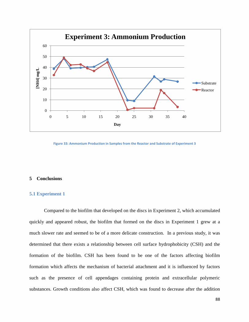
88
Figure 33: Ammonium Production in Samples from the Reactor and Substrate of Experiment 3
5 Conclusions
5.1 Experiment 1
Compared to the biofilm that developed on the discs in Experiment 2, which accumulated
quickly and appeared robust, the biofilm that formed on the discs in Experiment 1 grew at a
much slower rate and seemed to be of a more delicate construction. In a previous study, it was
determined that there exists a relationship between cell surface hydrophobicity (CSH) and the
formation of the biofilm. CSH has been found to be one of the factors affecting biofilm
formation which affects the mechanism of bacterial attachment and it is influenced by factors
such as the presence of cell appendages containing protein and extracellular polymeric
substances. Growth conditions also affect CSH, which was found to decrease after the addition
0
10
20
30
40
50
60
0 5 10 15 20 25 30 35 40
[NH
4]
mg
/L
Day
Experiment 3: Ammonium Production
Substrate
Reactor

89
of sodium chloride (NaCl) to the growth medium and this decrease resulted in the formation of
thinner and more fragile biofilms than those formed under high CSH conditions. Detachment
was observed to occur less frequently and on a smaller scale while the subsequent reattachment
and growth of the biofilm was found to be retarded under low CSH conditions.
This previous study reported that the hydrophobicity of bacterial cell colonies raised in a
substrate containing sodium chloride fell to zero faster than the hydrophobicity of bacterial
colonies grown in plain substrate did. It therefore appears that the sodium chloride must have
interacted with the bacteria in some manner, causing changes to their intrinsic hydrophobicity.
An increase in exopolysaccharide production, and hence a change in the cell physiology and the
cell surface properties, has been shown to occur in the presence of salts and this would lead to a
decrease in hydrophobicity if these exopolysaccharides are predominantly neutral or hydrophilic.
The effects on cell surface hydrophobicity caused by the alteration of the growth conditions
through the addition of sodium chloride, and consequently the effects on biofilm formation and
growth, can be attributed to this [51].
However, although it appears that the presence of sodium chloride in the substrate
affected the development and growth of the biofilm, whether the nitrifying properties of the
biofilm were affected could not be determined. The salt was added to the substrate before the
biofilm had been given an adequate amount of time to develop and mature and hence begin the
process of nitrification. Therefore, in the future, the biofilm will be allowed to grow on the discs
in the biological contactor for a longer period of time, the levels of nitrate and ammonia kept
under constant observation, and only when it is certain nitrification has begun will the sodium
chloride be added.
90
In previous experiments completed by Claire Perrin et al. in 2009, nickel has been shown
to increase the growth of biofilm when provided in moderate quantities. The addition of nickel to
a substrate results in an over expression of the curli gene in bacteria, specifically E. Coli. The
excess curli production converts certain bacteria from their natural planktonic form to a fixed
biofilm by inducing adherence of bacterial cells to one another. The belief is that the attachment
of the heavy metals to the EPS matrix of the biofilm protects the bacteria from the harmful
effects of the heavy metal. In pure culture studies, it has been found that biofilm grown cells are
two to six hundred times more resistant to metal stress than planktonic cells. This also relates to
the absorption capacity of the biofilm because it directly corresponds to the chelat-forming
capacity of the EPS matrix due to its inclusion of high numbers of carboxyl, hydroxyl, and acetyl
groups as well as ketal-linked pyruvates [52].
With respect to the biofilms being tested in this experiment, the increase of biomass due
to bacterial conversion from a planktonic state may explain the results of protein and COD
levels. Although the biomass of discs 1, 2, 4 and 5 steadily increased throughout the experiment
as shown by the measured opacity levels of the scans, the efficiency of the biofilms’ degradation
of organics decreased after day 59, when nickel was added to the system. The difference in levels
of both protein and COD between the water samples from the reactor and the substrate decreased
after day 59, indicating the deteriorating function of the biofilm as the addition nickel resulted in
a lower number of live cells that degrade these organic materials. In addition, it has been
observed that metal ions compete against organic compounds for active sites on biofilms
hampering organic degradation [53].
91
5.2 Experiment 2
The experiment with the fast rotating biological contactor, Experiment 2, demonstrated
that the application of a magnetic field and rotation speed affects biofilm development. On days
42 through 46, large portions of biofilm suddenly detached from the disc. The biofilm on the
discs inside of the magnetic field sloughed off about 2 days before the separation of the biofilm
from the disc outside of the magnetic field. Studies have shown that biofilm exposure to a
magnetic field results in transcriptional changes to planktonic cells, which affect the surface
adhesion of the free cells to the biofilm, resulting in dispersion and the rapid formation of denser
and thinner biofilm [49]. In comparison to a previous experiment by Marie Noëlle Pons, in
which a magnetic field was applied to biofilms rotating at a slower speed, biofilm detachment
occurred 5 to 7 days later than in Experiment 2. This may attributed to the velocity of the
rotating contactor, which resulted in shearing, or the constant elimination of small portions of the
biofilm.
The magnetic field also influences the biodegradation of organic materials in the
wastewater. Solutions exposed to magnetic fields readily absorb atmospheric oxygen. Due to
the fact that most microorganisms are aerobic, the increased oxygen concentration of the
magnetized wastewater results in more efficient metabolic activity and elimination of organic
materials. In addition, the increased oxygen concentration may result in the formation of free
radicals in the biofilm, which also reduce the concentration of organic matter [50]. The
reduction of organic materials through the increased oxygen concentration may have contributed
to the reduced COD and protein levels of the samples from the reactor compared to the samples
from the substrate of Experiment 2. However, there is no control experimental data available to
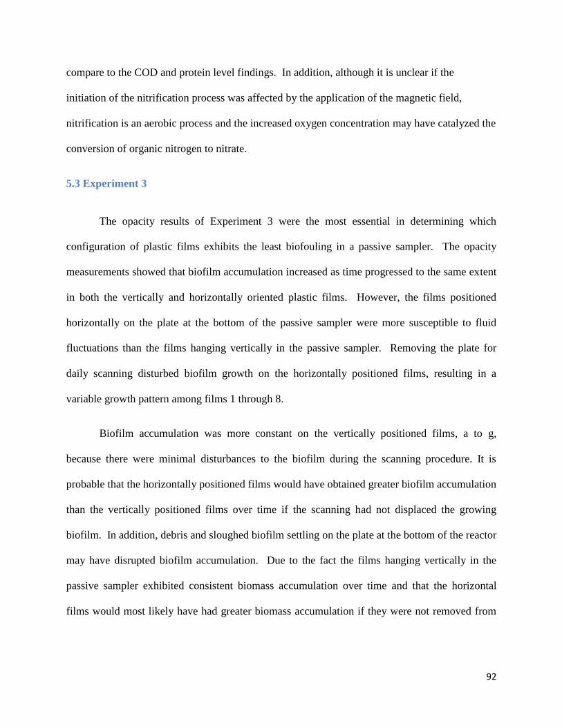
92
compare to the COD and protein level findings. In addition, although it is unclear if the
initiation of the nitrification process was affected by the application of the magnetic field,
nitrification is an aerobic process and the increased oxygen concentration may have catalyzed the
conversion of organic nitrogen to nitrate.
5.3 Experiment 3
The opacity results of Experiment 3 were the most essential in determining which
configuration of plastic films exhibits the least biofouling in a passive sampler. The opacity
measurements showed that biofilm accumulation increased as time progressed to the same extent
in both the vertically and horizontally oriented plastic films. However, the films positioned
horizontally on the plate at the bottom of the passive sampler were more susceptible to fluid
fluctuations than the films hanging vertically in the passive sampler. Removing the plate for
daily scanning disturbed biofilm growth on the horizontally positioned films, resulting in a
variable growth pattern among films 1 through 8.
Biofilm accumulation was more constant on the vertically positioned films, a to g,
because there were minimal disturbances to the biofilm during the scanning procedure. It is
probable that the horizontally positioned films would have obtained greater biofilm accumulation
than the vertically positioned films over time if the scanning had not displaced the growing
biofilm. In addition, debris and sloughed biofilm settling on the plate at the bottom of the reactor
may have disrupted biofilm accumulation. Due to the fact the films hanging vertically in the
passive sampler exhibited consistent biomass accumulation over time and that the horizontal
films would most likely have had greater biomass accumulation if they were not removed from

93
the reactor, it can be surmised that the vertical orientation is the best configuration in a passive
sampler.
The other analytical tests were less significant in determining the best orientation of the
plastic films. However, the results of these tests were indicative of the efficiency of the biomass
that formed on the plastic films. The lower protein concentration and Chemical Oxygen Demand
in the samples from the reactor than the samples from the substrate of Experiment 3
demonstrated that the biofilms were effectively removing organic materials from the water.
However, the results of the Ion Chromatography and Ammonium Test showed that the biofilm
had not matured enough to complete the nitrification process and to convert organic nitrogen into
nitrate. This may have been the result of the short duration of the experiment, the material the
biofilm was growing on, or environmental disturbances to the biofilm.
6 Appendices
6.1 Procedures
6.1.1 Maintenance of the Biological Contactors
Maintenance procedures were performed every other day on Runs 22, 23, and 24 to
replenish the substrate supply, which feeds each reactor; to remove any buildup that may affect
the functioning of the contactors; and to monitor the growth of the biofilms.
6.1.1.1 Procedure for the Maintenance of Experiment 1
1. Turn off the motor and the water pump that are associated with the rotating biological
contactor.
2. Remove the tubing connected to the RBC: the tubing which connects the water pump to
the glass contactor lid (the feed line), the tubing which connects the air pump to the lid
(the air line), and the third spacer tube (used only to keep the other two tubes in place).

94
3. Take the glass contactor lid off the apparatus.
4. Remove the screw which connects the axle to which the biodiscs are attached to an arm
that extends from the motor.
5. Gently lift the axle with the biodiscs and place it into a vice. Tighten the vice so that the
axle is secure.
6. Unfasten the outer screw. Carefully remove the small rubber spacers and the biodiscs,
placing each biodisc on a paper towel, biofilm side up, in a separate Petri dish.
7. Scan each biodisc according to the procedure described in the “Biofilm Scanning”
section.
8. Replace the biodiscs and the spacers on the axle in the correct order. Biodisc 1 is placed
on first, followed in numerological order up to biodisc 5. Reattach the end screw to
secure the biodiscs in place.
9. Before putting the axle back into the reactor, take a sample of water from the reactor
using a small, empty glass jar. Pour the water through a coffee filter placed in a funnel
and into a plastic sample container. Screw the cap on the container and label the container
with the run number, the date, and with the letter R for reactor. Place the sample in the
refrigerator.
10. Position the axle in the reactor and replace the screw that attaches the axle to the arm of
the motor.
11. Replace the glass lid of the reactor.
12. Connect the three tubes back to the glass lid. Every few days make sure to detach the
tubing completely from the apparatus and run water through it to clean it out.
13. Every two days, exchange the empty substrate container with a new container filled with
4.8 L of freshly made substrate (wastewater mixed with salt and heavy metals). Take a
sample from the substrate container and then filter and label it as described in step 9, but
with an S instead of an R.
14. Turn the water pump and the motor back on (the motor needs a little assistance to start
spinning).
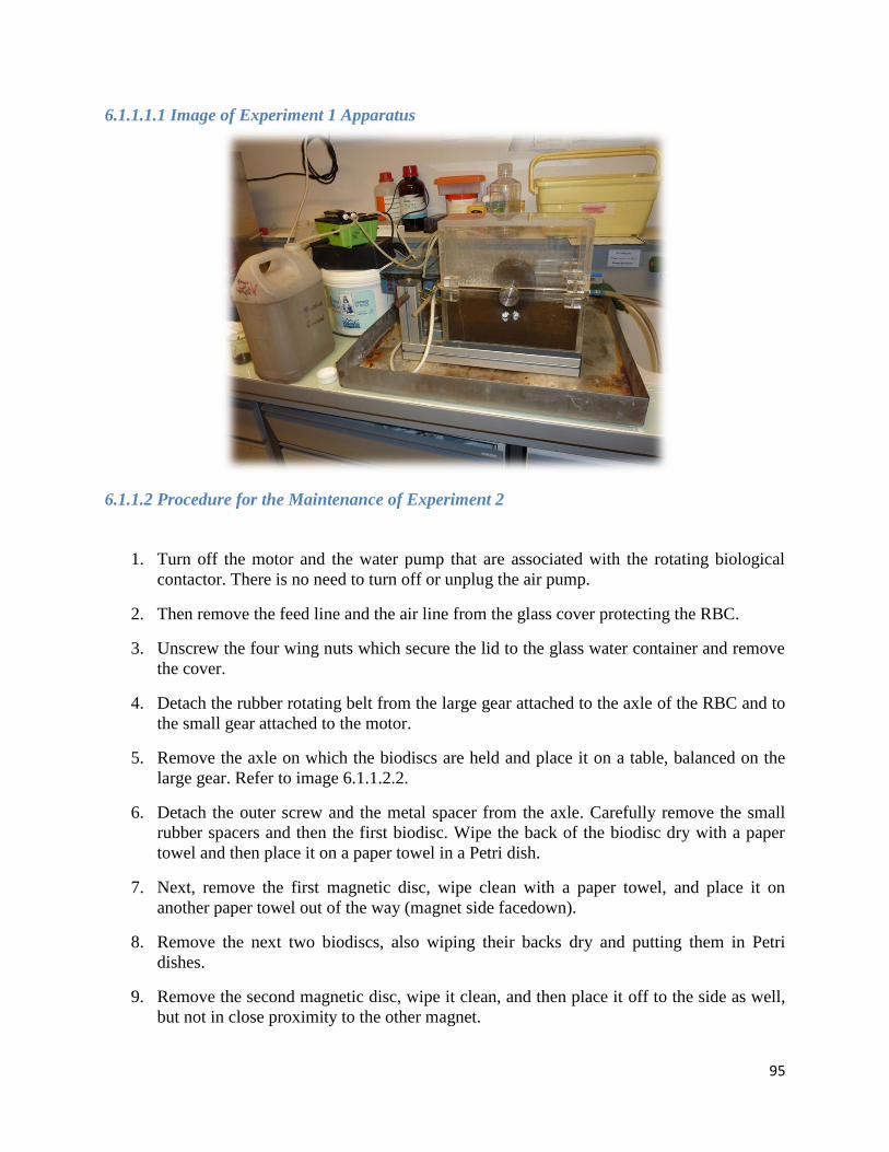
95
6.1.1.1.1 Image of Experiment 1 Apparatus
6.1.1.2 Procedure for the Maintenance of Experiment 2
1. Turn off the motor and the water pump that are associated with the rotating biological
contactor. There is no need to turn off or unplug the air pump.
2. Then remove the feed line and the air line from the glass cover protecting the RBC.
3. Unscrew the four wing nuts which secure the lid to the glass water container and remove
the cover.
4. Detach the rubber rotating belt from the large gear attached to the axle of the RBC and to
the small gear attached to the motor.
5. Remove the axle on which the biodiscs are held and place it on a table, balanced on the
large gear. Refer to image 6.1.1.2.2.
6. Detach the outer screw and the metal spacer from the axle. Carefully remove the small
rubber spacers and then the first biodisc. Wipe the back of the biodisc dry with a paper
towel and then place it on a paper towel in a Petri dish.
7. Next, remove the first magnetic disc, wipe clean with a paper towel, and place it on
another paper towel out of the way (magnet side facedown).
8. Remove the next two biodiscs, also wiping their backs dry and putting them in Petri
dishes.
9. Remove the second magnetic disc, wipe it clean, and then place it off to the side as well,
but not in close proximity to the other magnet.

96
10. Scan the biodiscs according to the “Biodisc Scanning” procedure.
11. Reassemble the biodiscs, the magnetic discs, and the spacers on the axle. Make sure that
the biodiscs are all placed back in the correct order. 1 is installed first followed in
numerological order up to 4, with the magnetic discs located between 1-2 and 3-4. The
magnets on the magnetic discs should be facing one another, so that discs 2 and 3 are
located in the magnetic field. There is also a small marking on discs 2-3 and both
magnetic discs; make sure to align these markings. Replace the end screw to secure the
biodiscs in place.
12. Before replacing the axle with the biodiscs in the RBC, use a small, empty glass jar to
collect some of the reactor water to test. Store the sample by following the procedure
described in step 9 of the “Procedure for Maintenance of Experiment 1”.
13. Gently place the axle back into the RBC container.
14. Reattach the rubber rotating belt and secure the cover back on with the wing nuts.
15. Reconnect all the tubing to the RBC. Every few days make sure to detach the tubing
completely from the apparatus and run water through it to clean it out.
16. At this point, every two days, replace the empty substrate container with a new container
filled with 4.8 L of freshly obtained wastewater. Take a sample from the substrate
container and then filter and label it as described in step 9 of the “Procedure for
Maintenance of Experiment 1”, but with an S instead of an R.
17. Turn the water pump and the motor back on
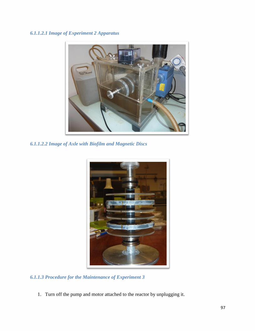
97
6.1.1.2.1 Image of Experiment 2 Apparatus
6.1.1.2.2 Image of Axle with Biofilm and Magnetic Discs
6.1.1.3 Procedure for the Maintenance of Experiment 3
1. Turn off the pump and motor attached to the reactor by unplugging it.
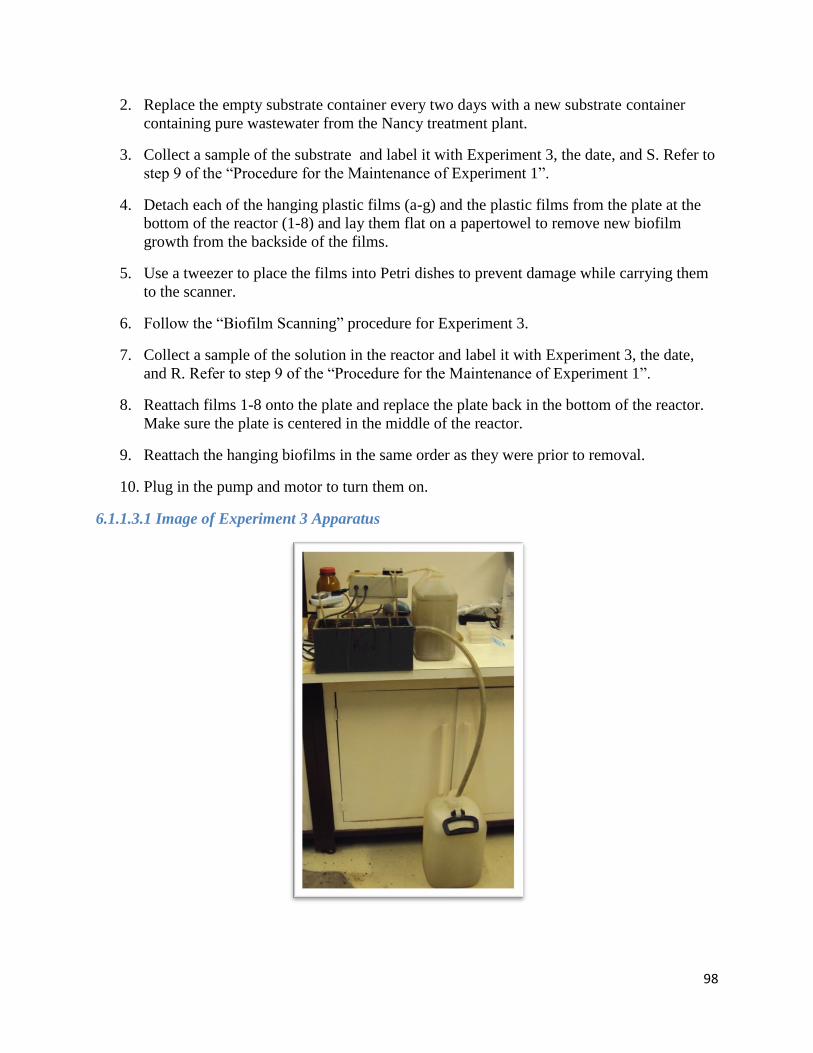
98
2. Replace the empty substrate container every two days with a new substrate container
containing pure wastewater from the Nancy treatment plant.
3. Collect a sample of the substrate and label it with Experiment 3, the date, and S. Refer to
step 9 of the “Procedure for the Maintenance of Experiment 1”.
4. Detach each of the hanging plastic films (a-g) and the plastic films from the plate at the
bottom of the reactor (1-8) and lay them flat on a papertowel to remove new biofilm
growth from the backside of the films.
5. Use a tweezer to place the films into Petri dishes to prevent damage while carrying them
to the scanner.
6. Follow the “Biofilm Scanning” procedure for Experiment 3.
7. Collect a sample of the solution in the reactor and label it with Experiment 3, the date,
and R. Refer to step 9 of the “Procedure for the Maintenance of Experiment 1”.
8. Reattach films 1-8 onto the plate and replace the plate back in the bottom of the reactor.
Make sure the plate is centered in the middle of the reactor.
9. Reattach the hanging biofilms in the same order as they were prior to removal.
10. Plug in the pump and motor to turn them on.
6.1.1.3.1 Image of Experiment 3 Apparatus
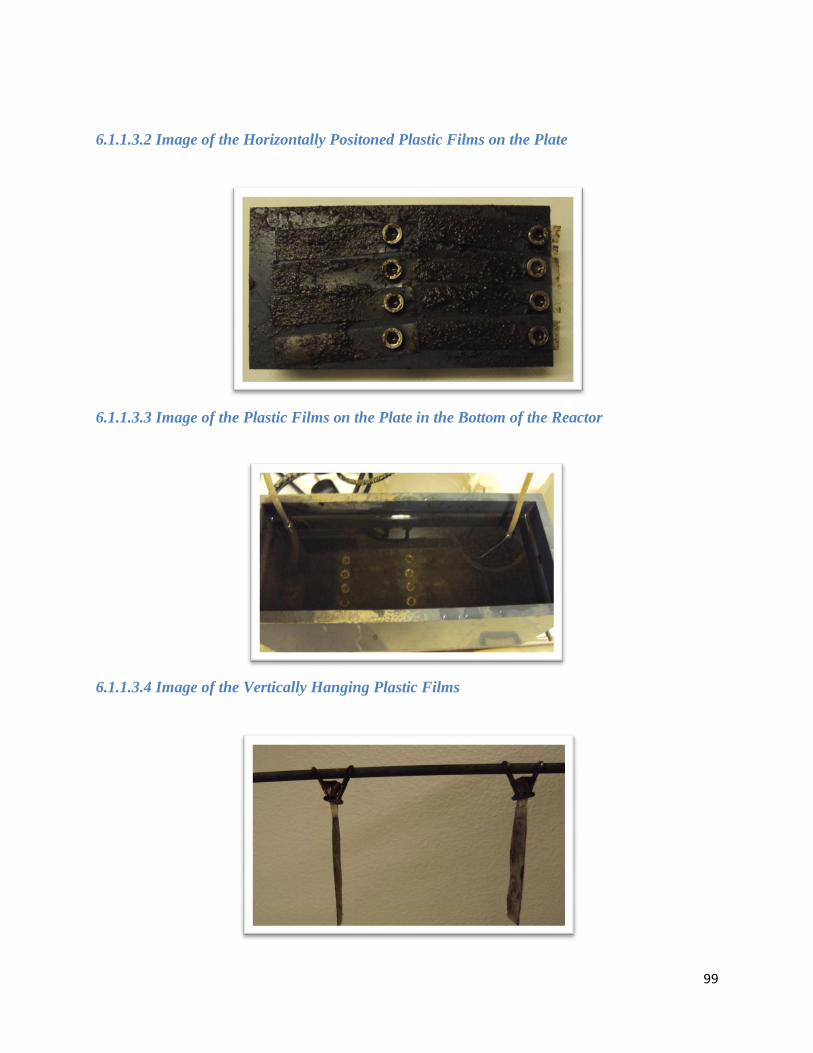
99
6.1.1.3.2 Image of the Horizontally Positoned Plastic Films on the Plate
6.1.1.3.3 Image of the Plastic Films on the Plate in the Bottom of the Reactor
6.1.1.3.4 Image of the Vertically Hanging Plastic Films
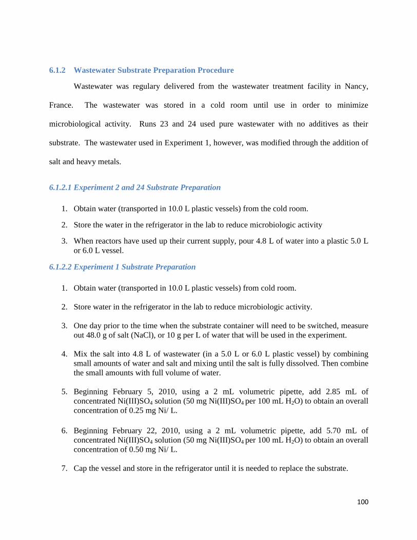
100
6.1.2 Wastewater Substrate Preparation Procedure
Wastewater was regulary delivered from the wastewater treatment facility in Nancy,
France. The wastewater was stored in a cold room until use in order to minimize
microbiological activity. Runs 23 and 24 used pure wastewater with no additives as their
substrate. The wastewater used in Experiment 1, however, was modified through the addition of
salt and heavy metals.
6.1.2.1 Experiment 2 and 24 Substrate Preparation
1. Obtain water (transported in 10.0 L plastic vessels) from the cold room.
2. Store the water in the refrigerator in the lab to reduce microbiologic activity
3. When reactors have used up their current supply, pour 4.8 L of water into a plastic 5.0 L
or 6.0 L vessel.
6.1.2.2 Experiment 1 Substrate Preparation
1. Obtain water (transported in 10.0 L plastic vessels) from cold room.
2. Store water in the refrigerator in the lab to reduce microbiologic activity.
3. One day prior to the time when the substrate container will need to be switched, measure
out 48.0 g of salt (NaCl), or 10 g per L of water that will be used in the experiment.
4. Mix the salt into 4.8 L of wastewater (in a 5.0 L or 6.0 L plastic vessel) by combining
small amounts of water and salt and mixing until the salt is fully dissolved. Then combine
the small amounts with full volume of water.
5. Beginning February 5, 2010, using a 2 mL volumetric pipette, add 2.85 mL of
concentrated Ni(III)SO4 solution (50 mg Ni(III)SO4 per 100 mL H2O) to obtain an overall
concentration of 0.25 mg Ni/ L.
6. Beginning February 22, 2010, using a 2 mL volumetric pipette, add 5.70 mL of
concentrated Ni(III)SO4 solution (50 mg Ni(III)SO4 per 100 mL H2O) to obtain an overall
concentration of 0.50 mg Ni/ L.
7. Cap the vessel and store in the refrigerator until it is needed to replace the substrate.
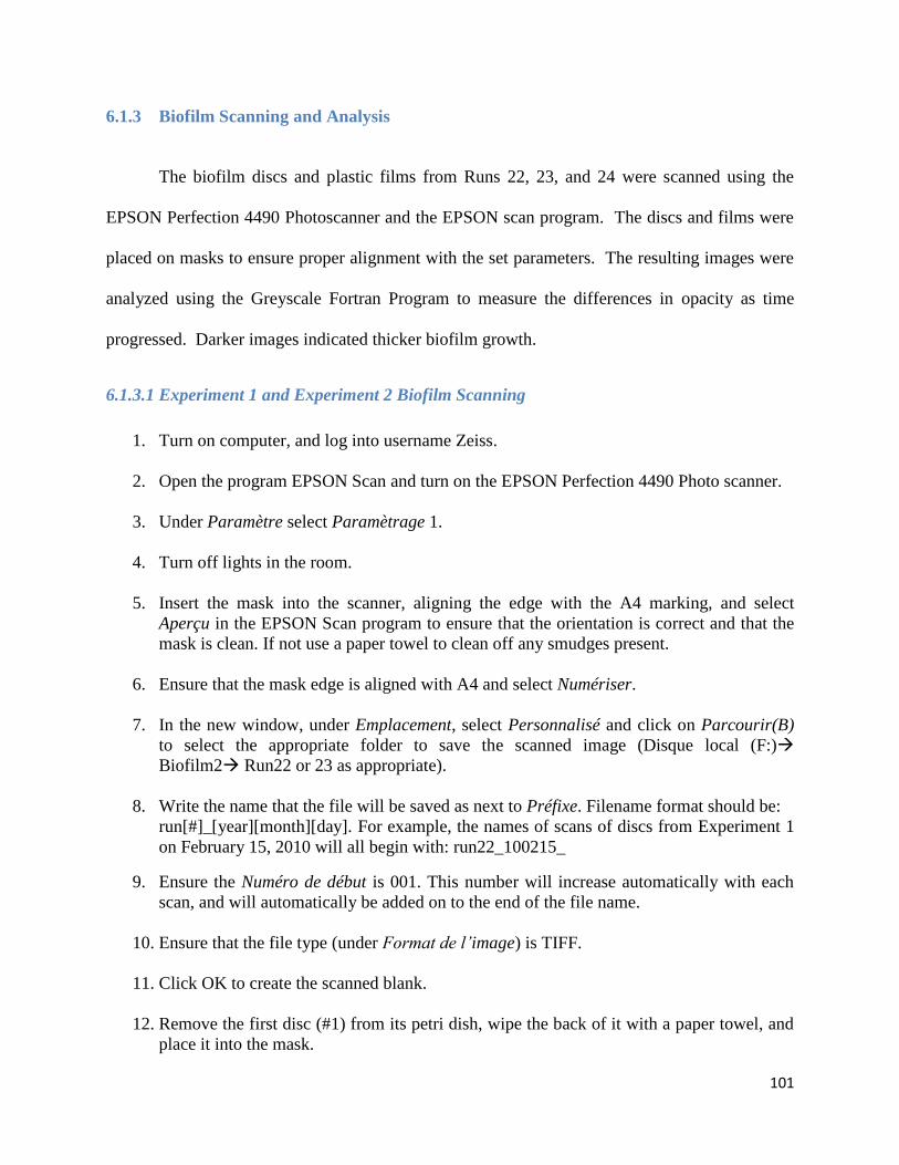
101
6.1.3 Biofilm Scanning and Analysis
The biofilm discs and plastic films from Runs 22, 23, and 24 were scanned using the
EPSON Perfection 4490 Photoscanner and the EPSON scan program. The discs and films were
placed on masks to ensure proper alignment with the set parameters. The resulting images were
analyzed using the Greyscale Fortran Program to measure the differences in opacity as time
progressed. Darker images indicated thicker biofilm growth.
6.1.3.1 Experiment 1 and Experiment 2 Biofilm Scanning
1. Turn on computer, and log into username Zeiss.
2. Open the program EPSON Scan and turn on the EPSON Perfection 4490 Photo scanner.
3. Under Paramètre select Paramètrage 1.
4. Turn off lights in the room.
5. Insert the mask into the scanner, aligning the edge with the A4 marking, and select
Aperçu in the EPSON Scan program to ensure that the orientation is correct and that the
mask is clean. If not use a paper towel to clean off any smudges present.
6. Ensure that the mask edge is aligned with A4 and select Numériser.
7. In the new window, under Emplacement, select Personnalisé and click on Parcourir(B)
to select the appropriate folder to save the scanned image (Disque local (F:)
Biofilm2 Run22 or 23 as appropriate).
8. Write the name that the file will be saved as next to Préfixe. Filename format should be:
run[#]_[year][month][day]. For example, the names of scans of discs from Experiment 1
on February 15, 2010 will all begin with: run22_100215_
9. Ensure the Numéro de début is 001. This number will increase automatically with each
scan, and will automatically be added on to the end of the file name.
10. Ensure that the file type (under Format de l’image) is TIFF.
11. Click OK to create the scanned blank.
12. Remove the first disc (#1) from its petri dish, wipe the back of it with a paper towel, and
place it into the mask.
102
13. Click Numériser and ensure that all options are the same as for the blank except for
Numéro de début, which should read 002.
14. Click OK.
15. After scanning is finished, return the disc to its Petri dish.
16. Repeat the process for the remaining discs in the proper order.
17. Once finished, close the program, log out of the computer, and turn off the scanner.
6.1.5.2 Experiment 1 and Experiment 2 Analysis
1. Turn on computer and log into username Zeiss.
2. Open Visilog 6.3.
3. Select File, Ouvrir, choose the folder containing the images of the run to be analyzed,
and choose the first image that will be analyzed (do not select number 001, the blank,
throughout the process).
4. Select the Point button on the toolbar, which appears as a blue set of intersecting lines.
5. Make three approximately equidistant points around the border of the scanned image of
the disc.
6. Click the Afficher les coordonnées des objets Point button, which appears as three red
points, two of which are connected to the third via red dotted lines. This will copy the
coordinates of the three points into a spreadsheet.
7. Close the image of the scanned disc and repeat the process with each scanned image for
that run.
8. Save the spreadsheet into the run’s folder as “coordinates[x].dat”, in which [x] is the
number of the time that the procedure has been carried out.
9. In the explorer, right click the file and open with Excel.
10. Add “.tif” to the end of all of the file names by, in a new column, entering:
=[cell of filename]&”.tif”.
11. All of the coordinates for points in each scan will be in a vertical column. Move the
coordinates so that they are in a horizontal row for each scan, before deleting the extra
rows from the spreadsheet, so that there is only one row for each scan file.
103
12. Copy the names that include “.tif” at the end into a new spreadsheet, and save this
spreadsheet in the run’s folder as “names.txt”.
13. Copy the point coordinates into a new excel spreadsheet and save this in the run’s folder
as “points.txt”.
14. Copy the entire run folder into the C: drive of the computer.
15. Ensure that the files “angles.txt” and “dists.txt” are in the folder. If not, copy and paste
them from a previous similar experiment.
16. Open the DOS Terminal (Invite de Commandes), and move back in directories by typing:
cd..
Once inside the directory containing the run folder, change to the appropriate directory by
typing (for Experiment 1, for example): cd run22
17. Open the grayscale Fortran program by typing: tex_disc_general
18. After each of the prompts, give the appropriate response:
Input file name: names.txt
Case: 2
Name of points file: points.txt
Min: 38
Max: 98
Name of stats file: stats_22.txt or stats_23.txt, as is appropriate.
Name of SGLDM file: sgldm_22.txt or sgldm_23, as is appropriate
Angle file: angles.txt
Distance file: dists.txt
Size of warped image: 1024
19. Open the new file “stats_22.txt” in excel, using delineated spacing, and add a new
column labeled “Opacity” with the following equation: =G$2-G2
*note: Use the values from the column labeled “Mean1”, which may not be G.
20. Drag this equation down to obtain the difference between the first entry of “Mean1” and
the following entries.
21. Organize the data in excel so as to group the data from each disc together.
6.1.5.3 Experiment 3 Biofilm Scanning
1. Turn on computer, and log into username Zeiss.

104
2. Open the program EPSON Scan and turn on the EPSON Perfection 4490 Photo scanner.
3. Under Paramètre select Paramètrage 7.
4. Turn off lights in the room.
5. Insert the mask into the scanner, aligning the edge with A4 marking, and select Aperçu in
the EPSON Scan program to ensure that the orientation is correct and the mask is clean.
If not use a paper towel to clean off any smudges present.
6. Ensure the mask edge is aligned with A4 and select Numériser.
7. In the new window, under Emplacement, select Personnalisé and click on Parcourir(B)
to select the appropriate folder to save the scanned image (Disque local (F:)
Biofilm2 Run24).
8. Write the name the file will be saved as next to Préfixe. Filename format should be:
run[#]_[year][month][day]. For example, the names of scans of discs from Experiment 3
on February 15, 2010 will all begin with: run24_100215_
9. Ensure the Numéro de début is 001. This number will increase automatically with each
scan, and will automatically be added on to the end of the file name.
10. Ensure the file type (under Format de l’image) is TIFF.
11. Click OK to create the scanned blank.
12. Remove the first plastic film (#1) from the plate, wipe the back of it with a paper towel,
and place it into the mask.
13. Click Numériser and ensure that all options are the same as for the blank except for
Numéro de début, which should read 002.
14. Click OK.
15. After scanning is finished, return the film to the plate.
16. Repeat the process for the remaining films in proper order (1-8 followed by a-h).
17. Once finished, close the program, log out of the computer, and turn off the scanner.
6.1.5.4 Experiment 3 Analysis
1. Turn on computer and log into username Zeiss.

105
2. Open the application ImageJ.
3. Select file, open, and choose the first scanned image from Experiment 3 (ignoring 001.
All files ending in 001 will be ignored)
4. Click on the Polygon Selections button, and click four points around the plastic slide to
surround it. In order to avoid unnatural artifacts in the perceived gray levels of the slide,
do not include in the selection the area of the slide with a hole (for those attached to the
plate on the bottom of the tank) or a letter (for those hanging from above the tank).
5. Select edit, then copy to system.
6. Select file, new, system clipboard.
7. Save the “cut” image as a TIF file in a subfolder of Run24 also called Run24. The name
of the image should be the same as it was before being cut.
8. To move to the next image to be cut, select file and open next. The rectangle made on the
previous image will appear again, and the corners may be dragged to appropriate
positions on the new image.
9. Copy the names that include “.tif” at the end into a new spreadsheet, and save this
spreadsheet in the run’s folder as “names.txt”.
10. Copy the entire run folder into the C: drive of the computer.
11. Ensure that the files “angles.txt” and “dists.txt” are in the folder. If not, copy and paste
them from a previous similar experiment.
12. Open the DOS Terminal (Invite de Commandes), and move back in directories by typing:
cd..
Once inside the directory containing the run folder, change to the appropriate directory by
typing (for Experiment 3, for example): cd Experiment 3
13. Open the grayscale Fortran program by typing: tex_disc_general
14. After each of the prompts, give the appropriate response:
Input file name: names.txt
Case: 2
Name of points file: points.txt
Minimum number of columns and rows:
400
1600
Name of stats file: stats_24.txt
Name of SGLDM file: sgldm_24.txt
Angle file: angles.txt
Distance file: dists.txt
106
15. Open the new file “stats_24.txt” in excel, using delineated spacing, and add a new
column labeled “Opacity” with the following equation: =G$2-G2
*note: Use the values from the column labeled “Mean”, which may not be G.
16. Drag this equation down to obtain the difference between the first entry of “Mean” and
the following entries.
17. Organize the data in excel so as to group the data from each film together.
6.1.6 Fluorescence Spectroscopy
Fluorescence spectroscopy was performed once a week on Runs 22, 23, and 24 in an
effort to estimate the relative amounts of organic materials in each of the samples of wastewater.
The objective was to determine whether there was a difference in the levels of the organic
materials between the reactor and substrate samples. The only peak that was pertinent to the
study was that of tryptophan, which is located at a wavelength 288 nm. The procedure for
fluorescence spectroscopy was:
1. Turn on the PC.
2. Log into the computer under Pons.
3. Turn on the Digilab Hitachi F-2500 fluorescence spectophotometer using the button on
the front of the device and make sure the lamp light turns on.
4. Open FL Solutions 2.0 on the desktop.
5. Set a baseline for the acquisition by loading a new method.
6. Load a new method. Click Method, Load, Program Files, FL Solutions, MNP, and then
raman_eau.flm.
7. Fill a plastic cuvet with deionized water.
8. Press Measure to obtain the reading.
9. Press Report and save the Excel file of the baseline.
10. Load a new method. Click Method, Load, Program Files, FL Solutions, MNP, and then
eau_sync.flm.
107
11. Rinse the plastic cuvette with the sample and then refill the cuvette with the same sample.
12. Press Measure to obtain the reading.
13. Press report and save the Excel file.
14. Close the windows and repeat steps 11 through 13 for each sample.
6.1.7 Ultraviolet-Visible Spectroscopy
Ultraviolet-Visible Spectroscopy was performed on samples from Runs 22, 23, and 24
each week. The purpose was to estimate the chemical oxygen demand (COD) for the substrate
and reactor samples. The peak at a wavelength of 254 nm corresponded to the COD
measurement. The procedure for Ultraviolet-Visible Spectroscopy was:
1. Turn the computer on. Login with the username ECCMA9. Do not start the LabPowerJ
software at this point.
2. Turn the UV-Vis Anthélie Light Spectrophotometer on (the switch is located on the
back). Allow the spectrophotometer to run its auto test.
3. When asked the question “Porte-cuve vide?”, check to make sure that the cuvette holder
is empty and then push the Val (validate) key.
4. When asked the question “Imprimer?” (Print), move the right arrow to Abandonner
(Abandon) and then push the Val key.
5. Once the auto test is finished, the word Absorbance will be indicated on the
spectrophotometer screen. Move the down arrow to the sub-menu Configuration and then
move the right arrow to Liaison RS232. Press the Val key.
6. Open the LabPowerJ software and prepare the program for spectra scanning.
7. Click on the sub-menu Méthode, then choose Nouvelle méthode, and finally choose
Balayage despectre.
8. Edit the parameters by clicking on éditer at the bottom of the main window. Change
Début (start) to 200 nm and Fin (end) to 600 nm.
9. Zero the spectrophotometer by first filling the quartz cuvette with DI water and then start
the baseline acquisition by clicking on OK. The device will tell how the baseline
acquisition is progressing.
10. Prepare the first sample by filling the quartz cuvette with the sample and then pouring it
out (to rinse the cuvette). Refill the cuvette with the sample, wipe it clean with a paper
towel, and then place it in the spectrophotometer.

108
11. Scan each sample by clicking on the yellow M icon in the LabPowerJ software.
12. Save the spectrum as an Excel file by choosing the export to excel option located under
the Fichier option in the menu bar of the main window.
13. Repeat steps 10 through12 for every sample.
6.1.8 The Ammonium Test
The concentration of ammonia was determined from the reactor and substrate samples
from Runs 22, 23, and 24 once a week. The samples were diluted 20 fold with the Hamilton
Digital Diluter in order to obtain an accurate reading with the Hach Spectrophotometer. The
samples were prepared using the Nesslerization process and the absorbance of each sample was
measured at 425 nm. The procedure for the Ammonium Test was:
1. Dilute each of the wastewater samples, both the substrate and reactor samples, 20 fold
using the Hamilton Digital Diluter.
Set the digital diluter to 90% and 50% (4.5 mL DI H20 and 0.5 mL sample).
Place the tube into the sample bottle and press the down arrow (the diluter will measure
the appropriate amount of both the DI water and the sample). Then place the tube into a
clean, empty test tube and press the up arrow to expel the two components of the diluted
sample into the test tube. The sample is now diluted 10 fold.
Then set the digital diluter to 99% and 0% to add 5 mL more of distilled water to dilute
the sample 20 fold.
Lastly, remember to make a blank sample. Use the machine while it is set to 99% and 0%
to add 10 mL of DI water to a test tube.
2. Add two drops of mineral stabilizer to each test tube, including the blank.
3. Add two drops of polyvinyl alcohol to each test tube, again including the blank.
4. Using an Eppendorf 100-1000 µL Manual Single Channel Pipet, add 400 µL Nessler’s
Reagent to each test tube.
5. Place caps on the test tubes and invert each tube several times to mix the sample.
6. Measure the absorption of each sample using a spectrophotometer set at a wavelength of
425 nm.
First zero the spectrophotometer using the blank. Wipe the test tube with a paper towel to
clean the glass and then place the tube into the machine. Choose the Signale Unique
109
option on the machine and then make sure that the wavelength is set t 425 nm before
pressing Zéro.
Test each sample in the same manner by first wiping off the test tube and then placing it
into the machine. However, for the samples instead of pressing Zéro press the Lire button
and record the absorbance.
7. To determine the ammonium concentration in each sample, use the calibration curve with
the equation y=3.651x with an R2 value of 0.999. Plug the absorbance value for each
sample into the following equation: [N·NH4] in mg/L = 3.651(Absorbance Value)*20. (It
must be multiplied by 20 to account for the 20 fold dilution).
6.1.9 Ion chromatography
Each week the samples from Runs 22, 23, and 24 were prepared to be run in the HPLC
machine by a trained laboratory technician. All of the samples were diluted 10 fold in order to
account for the high salt concentrations in Experiment 1 and in order to maintain comparable
data between the runs. The procedure for ion chromatography was:
1. Count the number of samples that will be tested.
2. Label 1.5 mL ion chromatography vials with numbers from ranging from 1 to the number
of samples.
3. Using the auto-dilution apparatus, combine 0.5 mL of the first sample with 4.5 mL of
deionized water (using the 90% and 50% settings for the 5 mL and 1 mL tubes,
respectively) to make a 90% diluted solution.
4. Using a 10 cc plastic syringe, remove the diluted sample.
5. Attach a 0.45 µm syringe filter and fill a labeled 1.5 mL vial.
6. Record the number of the vial and which sample it contains. Repeat for all of the
samples.
7. Store the sample vials in refrigerator until the ion chromatography test is to be carried
out.
The ion chromatography testing was carried out by Steve Pontvianne, the lab technician
at ENSIC. Once the diluted sample vials were prepared, they were delivered him the
results would be received by email or in person.

110
6.1.10 Inductively Coupled Plasma Atomic Emission Spectroscopy (ICP-AES)
Samples of the sludge taken from reactor of Experiment 1 were analyzed with ICP-AES
to test the heavy metal concentrations.
1. Using a small plastic handheld strainer, remove the sludge and sloughed biofilm from the
bottom of the tank, creating minimal turbulence. If turbulence is created and biofilm is
kicked up into the water, remove as much as possible, depositing into small glass jar.
2. Without attaching a lid, place the jar into an oven at 105ºC for 24 hours to fully dehydrate
the sludge.
3. Using a metal scraping implement, remove dried sludge from the jar. Ensuring the dried
sludge is fully crushed, without flakes, transfer to a labeled plastic vial and cap the vial.
4. Deliver vial to be analyzed via ICP-AES

111
Work Cited
1. The History of Wastewater Treatment [Online]. Available from:
http://www.cityoflewisville.com/wcmsite/publishing.nsf/AttachmentsByTitle/Wastewater
+Treatment+History/$FILE/The+History+of+Wastewater+Treatment3.pdf. Accessed
2010 Jan 20.
2. Henze M, Herremoë P. 2002. Wastewater Treatment: Biological and Chemical Processes.
3rd
ed. New York: Springer.
3. McRandle PW. 2007. What Happens to Pharmaceuticals in Wastewater? National
Geographic Green Guide. 122.
4. Villares R, Carballeira A. 2006. Trophic Categorization in the Rías Baixas (NW Spain):
Nutrients in Water and in Macroalgae. Scientia Marina. 70: 89-97.
5. Harshman V, Barnette T. 2010. Wastewater Odor Control: An Evaluation of
Technologies [online]. Available from: http://www.wwdmag.com/Wastewater-Odor-
Control-An-Evaluation-of-Technologies-article1698. Accessed 2010 Jan 25.
6. Omoike A, Vanloon G. 1999. Removal of Phosphorous and Organic Matter Removal by
Alum During Wastewater Treatment. Water Res 33:3617-3627
7. Vesilind P. 2003. Wastewater Treatment Plant Design. IWA Publishing. Alexandria, VA.
8. Tchobanoglous G, Burton F, Stensel H. 2002. Wastewater Engineering: Treatment and
Reuse. 4th
ed. New York: McGraw-Hill Science/Engineering/Math.
9. Lens P, Pol L, Wilderer P, Asano T. 2002. Water Recycling and Resource Recovery in
Industry: Analysis, Technologies and Implementation. Padstow, Cornwall, UK: TJ
International (Ltd). p. 359-370.
10. Donian, RM 2002. Biofilms: Microbial Life on Surfaces. Emerging Infectious Diseases.
8: 881-890
11. Wesley SG, Satheesh S. 2009. Temporal variability of nutrient concentration in marine
biofilm developed on acrylic panels. Journal of Experimental Marine Biology and
Ecology. 379: 1-7.
12. Reynolds K. 2008. New Clues in Understanding Biofilm Formation. Water Conditioning
and Purification.
13. Romeo T. 2008. Bacterial Biofilms. Berlin: Springer Verlag. p. 254-260
14. Kurladze GV. 2007. Environmental Microbiology Research Trends. New York: Nova
Science Publishers, Inc. p. 107-110
15. Kjelleberg S, Givskov M. 2007. The Biofilm Mode of Life: Mechanisms and
Adaptations. Norfolk, UK: Horizon Bioscience. p. 25-26, 46-49.
16. Laskin AI, Bennett JW, Gadd GM. 2005. Advances in Applied Microbiology Volume 57.
San Diego, CA: Elsevier Inc. p. 81-104, 165-175
17. Evans, LV. 2000. Biofilms: recent advances in their study and control. Amsterdam:
Overseas Publishers Association. p. 43
18. Melo, LF. 1992. Biofilms: Science and Technology. Norwell, MA: Kluwer Academic
Publishers. p. 150
19. Todar, K. 2008. Online Textbook of Bacteriology: Pseudomonas aeruginosa [online].
Available from: http://www.textbookofbacteriology.net/pseudomonas.html. Accessed 2010
Jan 20. 20. Andersson S, Rajarao GK, Land CJ, Dalhammar G. 2008. Biofilm formation and
interactions of bacterial strains found in wastewater treatment systems. FEMS
Microbiology Letters. 283: 83-90

112
21. Fried J, Mayr G, Berger H, Traunspurger W, Psenner R, Lemmer H. 2000. Monitoring
protozoa and metazoa biofilm communities for assessing wastewater quality impact and
reactor up-scaling effects. Water Science and Technology. 41: 313
22. Vogel AI. 1989. Textbook of Quantitative Chemical Analysis. 5th
ed. New York: John
Wiley and Sons Inc. p. 731-733.
23. Dekker M, Guilbault GG. 1990. Practical Fluorescence. 2nd
ed. New York: Marcel
Dekker, Inc.
24. Valeur B. 2002. Molecular Fluorescence: Principles and Applications. Weinham: Wiley-
VCH.
25. Pokalsky, C, Wick P, Harms E, Lytle FE, Van Etten RL. 1995. Fluorescence Resolution
of the Intrinsic Tryptophan Residues of Bovine Protein Tyrosyl Phosphatase. The Journal
of Biological Chemistry. 270: 3809-3815.
26. Edwards VA. The Nitrogen Cycle- Control Ammonia and Nitrate in Ponds, Lakes,
Lagoons, Rivers, and Wastewater Treatment [Online]. Available from: http://www.alken-
murray.com/BioInfo2-03.htm. Accessed 2010 Jan 20.
27. Ammonia (nitrogen) [Online]. Available from: http://www.chemetrics.com/analytes/
ammonia.html. Accessed 2010 Jan 20.
28. Hach CC, Brayton SV, Kopelove AB. 1985. A powerful Kjeldahl nitrogen method using
peroxymonosulfuric acid. Journal of Agricultural and Food Chemistry. 33(6): 1117-1123
29. Robinson JW. 2005. Undergraduate Instrument Analysis. New York, NY. Marcel
Deckker Inc. p. 178-230
30. Martins AF, Arsand DR, Brenner CB, Minetto LM. 2008. COD Evaluation of Hospital
Effluent by Means of UV-Spectral Deconvolution. Clean-Journal. 36(10-11): 875-878
31. Reynold DM, Ahmad SR. 1997. Rapid and Direct Determination of Wastewater BOD
Values Using a Fluorescence Technique. Wat. Res. 21(8): 2012-2018.
32. Worley J, Kvech K. 2000. ICP-MS [Online]. Available from: http://www.cee.vt.edu/
ewr/environmental/teach/smprimer/icpms/icpms.htm. Accessed 2010 Feb 3.
33. Da Silva M, Nascimento A, Da Silva V, Pons M, Da Motta M. 2009. Evaluation of
Bioaugmentation Efficiency for the Treatment of Run-Off Water Under Tropical
Conditions: Applications to the Derby-Tacaruna Canal. Water Science and Technology.
60
34. Vrana B, Mills G, Allan I, Dominiak E, Svensson K, Knutsson J, Morrison G,
Greenwood R. 2005. Passive sampling techniques for monitoring pollutants in water.
Trends in Analytical Chemistry. 24: 845-868.
35. Zabiegała B, Kot-Wasik A, Urbanowicz M, Namieśnik J. 2009. Passive sampling as a
tool for obtaining reliable analytical information in environmental quality monitoring.
Analytical Bioanalytical Chemistry. 396: 273-278.
36. Namiesnik J, Szefer P. 2010. Analytical Measurements in Aquatic Environments. Boca
Raton, FL: CRC Press. p. 49
37. Francesc A, Turrilla E, Yusà V, Pastor A, Guardia M. 2007. New perspectives in the use
of semipermeable membrane devices as passive samplers. Talanta. 74: 453-455
38. Petzoldt T, Uhlmann D. 2006. Nitrogen emissions into freshwater ecosystems: Is there a
need for nitrate elimination in all wastewater treatment plants? Acta Hydrochim.
Hydrobiol. p. 305-324
39. White J, Reddy K. 2003. Nitrification and Denitrification Rates of Everglades Wetland
Soils Along a Phosphorus-Impacted Gradient. J Environ Qual. 32

113
40. Lewandowski Z, Beyenal H. 2007. Fundamentals of Biofilm Research. New York: CRC
Press. p. 103
41. Inductively Coupled Plasma-Atomic Emission Spectrometry (ICP-AES) [Online]. 2008.
Koninklijke Philips. Available from: http://www.miplaza.com/materialsanalysis
/projects/technical noteschemicalanalysis/icpaesan.pdf. Accessed 2010 Feb 8.
42. Marine Science: Seawater Composition [Online]. 2008. Available from: http://www.
marinebio.net/marinescience/02ocean/swcomposition.htm. Accessed 2010 Feb 2.
43. Pederson K. 1982. Factors Regulating Microbial Biofilm Development in a System with
Slowly Flowing Seawater. Applied and Environmental Microbiology. 44(5): 1196-1204
44. Teitzel GM, Parsek MR. Heavy Metal Resistance of Biofilm and Planktonic
Pseudomonas aeruginosa. Applied and Environmental Microbiology. 69(4): 2313-2320
45. Chen F, Xia Q, Ju L. 2003. Aerobic Denitrification of Pseudomonas aeruginosa
Monitored by Online NAD(P)H Fluorescence. Appl Environ Microbiol. 69(11): 6715–
6722.
46. Vivian JT, Callis PR. 2001. Mechanisms of Tryptophan Fluorescence Shifts in Proteins.
Biophysical Journal. 80: 2093-2109.
47. Reynolds DM, Ahmad SR. 1995. The Effect of Metal Ions on the Fluorescence of
Sewage Wastewater. Wat. Res. 29(9): 2214-2216
48. Oxford A. Chemistry and the Nitrogen Cycle [Online]. Available from: http://www.ala
skafb.org/~akaitc/alaskaAITC/pdf/9_12/chemistry_nitrogen.pdf. Accessed 2010 Feb 20.
49. Di Campli E, Di Bartolomeo S, Grande
R, Di Giulio M, Cellini L. 2009. Effects of
Extremely Low-Frequency Electromagnetic Fields on Helicobacter pylori Biofilm.
Current Microbiology.
50. Krzemieniewski M, Dębowski M, Janczukowicz W, Pesta J. 2004. The Influence of
Different Intensity Electromagnetic Fields on Phosphorus and COD Removal from
Domestic Wastewater in Steel Packing Systems. Polish Journal of Environmental
Studies. 13(4): 381-387
51. Kuntiya A, Nicolella C, Pyle L, Poosaran N. 2005. Effect of sodium chloride on cell
surface hydrophobicity and formation of biofilm in membrane bioreactor. Songklanakarin
J. Sci. Technol. 27(5): 1073-1082
52. Perrin C, Briandet R, Jubelin G, Lejeune P, Mandrand-Berthelot M, Rodrigue A, Dorel
C. 2009. Nickel Promotes Biofilm Formation by Escherichia coli K-12 Strains That
Produce Curli. Applied and Environmental Microbiology. 75(6): 1723-1733
53. Lawrence JR, Chenier MR, Roy R, Beaumier D, Fortin N,. Swerhone GDW, Neu TR,
and Greer CW. 2004. Microscale and Molecular Assessment of Impacts of Nickel,
Nutrients, and Oxygen Level on Structure and Function of River Biofilm Communities.
Applied Environmental Microbiology. 70(7): 4326–4339


