
The development and application ofan LHD underground face simulator
Item Type text; Thesis-Reproduction (electronic)
Authors Mazaris, George Michael
Publisher The University of Arizona.
Rights Copyright © is held by the author. Digital access to this materialis made possible by the University Libraries, University of Arizona.Further transmission, reproduction or presentation (such aspublic display or performance) of protected items is prohibitedexcept with permission of the author.
Download date 27/07/2018 00:44:28
Link to Item http://hdl.handle.net/10150/557654

THE DEVELOPMENT'AND APPLICATION OF
AN LHD UNDERGROUND FACE SIMULATOR
by
George Michael Mazaris
A Thesis Submitted to the Faculty of the
DEPARTMENT OF MINING AND GEOLOGICAL ENGINEERING
In Partial Fulfillment of the Requirements For the Degree of -
. • MASTER.OF SCIENCE -- WITH A MAJOR IN MINING ENGINEERING
In the Graduate College
THE UNIVERSITY OF ARIZONA^
1 9 8 1

STATEMENT BY AUTHOR»
This thesis has been submitted in partia l fulfillment of re q u ire ments for an advanced d eg ree at The U niversity of Arizona and is deposited in the U niversity L ib ra ry to be made available to borrow ers u n d e r rules of the L ib ra ry .
Brief quotations from th is thes is a re allowable without special permission, provided th a t accu ra te acknowledgment of source is made. R equests for permission for ex tended quotation from or reproduction of th is m anuscrip t in whole or in p a r t may be g ran ted by the head of the major departm ent or the Dean of the G raduate College when in his ju d g ment the proposed use of the material is in the in te re s ts of schola rsh ip . In all o th e r in s tances , however, permission must be obtained from the au th o r .
SIGNED:
APPROVAL BY THESIS DIRECTOR
This thesis has been approved on the date shown below:
______ ^ / / J & /Y. C. KIM Date
P ro fesso r of Mining and Geological Engineering

ACKNOWLEDGMENTS
The author of this thesis would like to express his appreciation
to those individuals whose comments helped in its creation. A debt of
gratitude is owed to Dr. Y. C. Kim, thesis advisor, whose collaboration
and remarks helped to put the various ideas into an explicit and con
tinuous form. Professors T. J. O'Neil and J. C. Dotson are acknowledged
for serving on the thesis committee and for their helpful critiques. The
management of the S & S Corporation, Green Bluffs, Virginia, is thanked
for providing the data used in the application of the model. Special
thanks are given to Miss Julie Cameron for her helpful corrections of the
first draft and to H. R. Hauck for assistance in the preparation of the
final draft.

TABLE OF CONTENTS
Page
LIST OF ILLUSTRATIONS ........................ vi
LIST OF T A B L E S . vii
ABSTRACT ........................ viii
INTRODUCTION ............................................ . 1
Statement of the Problem . . . . . . . . . . . . . . . . . . . 1Load-Haul-Dump E quipm ent.................................................................... 2
Machine D escrip tion ................... 2Advantages and Disadvantages . ................................................ 4
Application of LHD- Equiopment in M ining................................ 6Review of Currently Available Face Simulation Programs . . . . . 7Purpose and Scope ................................................................ . 11
METHOD OF ANALYSIS . . . . . . . . . . . . . . . . . . . . . . 12
Simulation Philosophy ............................................ 12Simulation in Underground Mining S y ste m s......................... 15Simulation Program MINPIL. . . . . . . . . . . ............................ 16
Input Variables ................................ 17O u tp u t .................... 23Simulation Procedure........................ . 23
Program Capabilities . . . . . . . . . . . . . . . . . . . . . . 32Deterministic Simulation ............................................ 32Range of V a r ia b le s ............................ 32Assumptions Used in the Model.................... 32
VALIDATION OF PROGRAM MINPIL................................ 34
APPLICATION OF PROGRAM MINPIL . ; ................... . . . '................. 49
Program Adjustment • . ............................................ 49Results of Program Application................................................................. 53
Productivity Estimation , 53Analysis of Sensitivity of Productivity
to Average Haul Speed ............................. 55
CONCLUSIONS.................................... 56
Capability of Program MINPIL to HandleVaried Operating Characteristics ............................................ 56
iv

V
TABLE OF CONTENTS—Continued
Page
Room-and-Pillar Mine Layout P rob lem s........................................ 56General LHD A p p lica tio n s.................................................... 57
Suggested Refinements. . . . ............................ 57
APPENDIX A: PROGRAM MINPIL INPUT AND OUTPUT FOR SIMULATION STUDY OF LHD OPERATIONS IN FIVE COAL MINES................................ 59
APPENDIX B : INPUT AND OUTPUT DATA FOR SENSITIVITYANALYSIS STUDY ........................ 72
APPENDIX C: USER'S MANUAL FOR PROGRAM MINPIL........................ 91
REFERENCES 164

LIST OF ILLUSTRATIONS
Figure Page
1. Increasing trend of use of LHD equipment inunderground mines . . ................................ 3
2. Basic parameters for a typical room-and-pillar panel . . . . 20
3. Sequence of cuts with which program MINPIL cansimulate a typical adit development................................ 21
•4. Sequence of cuts with which program MINPIL can5 simulate a typical pile removal . . . . . . . . . . . . . . 22
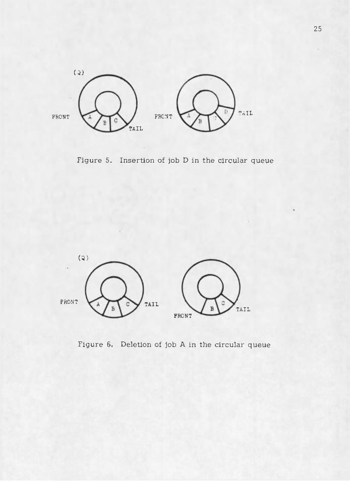
5. Insertion of job D in the circular queue . .............................. 25
6. Deletion of job A in the circular queue . . . . . . . . . . . 25
7. Main events of the program MINPIL circular queue . . . . . 26
8. Method by which program MINPIL examinesavailability of the called unit. . . . . . ' ..................... 31
9. Status of the five runs of Case 1 . . .......................................... 35
10. Average LHD queueing, down, and waiting timesfor the five runs of Case 1 37
11. Results of Case 1 .......................... 38
12. Status of the five runs of Case 2 ........................................... 40
13. Average LHD queueing, down, and waiting timesfor the five runs of Case 2 41
14. Results of Case 2 ......................................... 42
15. Results of the five runs of Case 3 ......................... .44
16. Three-dimensional diagram showing the resultsof joint sensitivity analysis . . . . . . . . . . . . . . . 45
17. Room-and-pillar panel used for Case 4 . . . . . .................. 47
vi

LIST OF TABLES
Table Page
1. Advantages and Disadvantages of LED Units . . . . . . . . 5
2. Program MINPIL Input Variables . ..................................... ... . 10
3. Program MINPIL O u tp u t.................... 23
4. Individual Run Statistics for Case 4 . . .................................. 48
5. Summary of Input Data for Operational LED U nits........... 51
6. Summary of Productivities and Rankings of LED Models . . . 52
vii

ABSTRACT
Introduction of high mechanization in underground mines has re
sulted in replacement of conventional methods in stoping and development
operations. Load-haul-dump (LHD) units with their high productivity,
flexibility, and low maintenance cost have been introduced into mines
using room-and-pillar, mechanized cut-and-fill, sublevel caving, and
stoping methods and for development work.
A computer program, written in FORTRAN and using an event-
oriented simulation philosophy, was developed to simulate LHD operation
between a series of discrete quantities of material (the mining cut) and
a dumping point. A combination of appropriate cut tonnage and selected
sequence for mining the cuts permits simulation of LHD operation under
the desired mine plan.
The program was validated with test data and then applied to a
specific real problem of estimating productivity for different models of
LHD units opearating under similar conditions. The four methods for
estimating productivity available in the program were analyzed, and it
was found that for the problem the productivity measured in kilometer-
tons per minute gave a reliable estimate. The sensitivity of the model
to characteristics of LHD units and mining operations was demonstrated
by using the sensitivity analysis option of the program to determine the
effect of average haul speed on production per shift.
viii
INTRODUCTION
Statement of the Problem
The present turmoil in the world economy has not left out one of
its most capital-intensive members, the mining industry. The frequent
economic fluctuations have caused an increase in the cost of mining oper
ations. The problem becomes more critical in underground mining where
mining costs are undoubtedly higher than costs of surface operations.
The reduction or even closure of operations in an underground mine be
cause of high costs is not an unusual phenomenon in the mining world.
To curb the disadvantages that derived from economic instability,
mine management is trying to invent, develop, and apply hew cost-
reducing tools. The first step in solving the problem is to point out
possible sources of high costs in operations. This is not difficult. An
experienced miner can easily point out that the main sources of high
costs in underground activities are the working faces. The second step
is to determine the measure to take to decrease mining costs. In general,
such efforts involve development of new, more efficient, mechanized min
ing methods and the introduction of more productive machinery. Selecting
the right equipment for the appropriate mining method may cut down the
cost of mining considerably and thereby contribute to the solution.
But the problem is not solved yet. Although new methods or new
equipment may theoretically reduce cost, their behavior in a specific mine
is still unknown. Considering the high price of a new machine or a method
change, mine management confronts the problem of finding ways toV -

2
appraise the new situations in advance in order to justify the large in
vestment involved.
Load-Haul-Dump Equipment
Application of mechanized underground stoping and development
operations has substantially contributed to underground mine production.
The use of trackless mining equipment, which is the major component of a
mechanized underground method, has shown a tremendous increase since
the early 1960s. Equipment like load-haul-dump (LHD) units, mobile
haulage units, and ancillary support vehicles have become common opera
tional units in the mines of Africa, Australia, Canada, Europe, the Middle
and Far East, South America, and the United States.
Historically, the use of LHD units represents the greatest change
in underground rock handling since the introduction of the mechanized
loader in the mid 1930s (Johnstone, 1975b, p. 44).
At first, operation of LHD units was confined to development of
horizontal tunnels. Later, due to mobility and development of efficient
exhaust systems, the units were introduced to stoping operations.
Figure 1 illustrates the growth over time of the total number of mines
that use LHD equipment.
Machine Description
An LHD unit is a center-articulated loader that can perform the
loading, hauling, and dumping activities and is composed of two subunits:
1. A truck, powered by a diesel or hydrostatic motor,, which contains
all the operational systems and the driver's seat.

:n e s
140
120
100
8 0
6 0
40
20
0
Figi
+ + + UPTURN PO IN T : 1 9 6 5
+
♦
+
51 1 9 5 5 1 9 5 9 1 9 6 3 1 9 6 7 1971 1 9 7 5
1. Increasing trend of use of LHD equipment in under-

4
2. The bucket, which is operated by hydraulic or compressed air.
A good description of an LHD unit is given by Knopp (1975,
p. 51):
Take a conventional front end loader, place one hand on top, the other on the bottom, and squeeze—but don't let it get any wider.The resulting altered silhouette illustrates the basic difference between the short, high front end loader and the lower, longer load-haul-dump [u n it]. While the load-haul-dump [unit] doesn't offer the top travel speeds, maneuverability or dump clearance of its above the ground cousin, pound for pound it offers 50 percent greater bucket capacity, a slightly smaller engine and generally better exhaust emission characteristics.
Advantages and Disadvantages
The following discussion on the advantages and disadvantages of
the LHD equipment is primarily based on the answers of the 119 mines
that took part in the investigation about LHD units made by Mining
Magazine- (Johnstone, 1975b, pp. 45-53).
The LHD units have been used in a variety of mines because of
the advantages they have, but it should not be though that this loading
system is a panacea for underground operations. These units do have a
lot of disadvantages, which sometimes may be critical and result in their
rejection. The specific advantages;and disadvantages are summarized in
Table 1.
The most important advantage, as the survey pointed out, is the
high productivity of the LHD unit. The gain in productivity results in
reduced costs of production, better efficiency, and ease of labor recruit
ment. Flexibility, mobility, and versatility were mentioned with enthusiasm.
Development speed and cost were also rated high.

5
Table 1. Advantages and Disadvantages of LED Units
Advantages Disadvantages
Eigh productivity Ventilation problems with diesel-powered LES units
FlexibilityEigh maintenance costs and time
Eigh productionLow average availability
MobilityShortage of skilled manpower
VersatilityEigh capital investment
Development speed and costGround control required
Ease of incline development
Adaptability to mining methods
Improved ore recovery
Wide choice of equipment
The high productivity derives from the adaptability, mobility,
better visibility, and good traction of LED units due to the following
LED characteristics:
1. Long, narrow, low profile (adaptability).
2. Center articulation (mobility).
3. Center sideways position for operator (better v isib ility ).
4. Rubber tires (mobility).
5. Planetary axles (support for heavy loads).
6. Four-wheel drive (better traction).
7. Equal speeds in both directions (mobility).

6
Most of the operators of the mines participating in the survey
pointed out that the main disadvantage to the use of LHD units is the
cost of the increased ventilation required when diesel-powered units are
used. As is stated in the results of the survey (Johnstone, 1975a, p.
115): "Although the various cleaners for exhaust fumes have been an
object of concentrated concern and research over the past few years . . .
the mine operators find the extra ventilation requirements irksome." The
ventilation problem has caused a complete rejection of the diesel-powered
LHD equiopment in many mines.
The high maintenance cost and low.availability are a result of the
high sophistication of LHD equipment and the low availability of spare
parts in some places in the world. The shortage of skilled manpower may
create economic problems because exhaustive and extensive training is
needed to become familiar with the equipment. The required ground con
trol was, in the opinion of the operators of the mines participating in the
survey, a major disadvantage. The large excavations needed to accom
modate the equipment and the requirement for good road conditions to
increase equipment traction impose extra costs.
Application of LHD Equipment in Mining
The results of the survey reported by Johnstone (1975b) show
that many of the world's hard-rock mines use LHD equipment. Further
more, many operators have found that using LHD units is far more pro
ductive than using the conventional trackless system of shuttle cars
with conveyors, if the tramming distance for the LHD units is kept within
economical limits. These limits are unique for each mine and depend on

the parameters (speed, ground control, existing water conditions, e tc .)
of the specific operation.
Specifically, LHD equipment has been reported to operate in open
sloping and inclined room and pillar (Clark, 1973), sublevel caving and
sloping, block caving, mechanized cut and fill, vertical crater retreat,
breast sloping, top slice, undercut and fill, long-hole benching, square
set, and development work.
The introduction of LHD equipment in an existing mine may re
quire changes in existing operations. For. example, when INCO's
Creighton mine in Canada introduced LHD equipment in 1966 to replace
the existing slusher cleaning method, it was necessary to develop a ramp
between the various levels so that the LHD units could move easily be
tween levels (Parris, 1969). The choice of LHD equipment for a new mine
may be influenced by economic factors. Prieska Copper Mines Ltd.'s
choice of LHD units for development of a new mine was determined by the
relatively high cost of electric power in the area in which the mine was
located.
Review of Currently Available Face Simulation Programs
The high complexity and variability of face operations and the
increased availability of computer facilities and the accuracy of their
answers have prompted many engineers and programmers to develop
simulation programs to examine underground material handling systems
(Subolesky and Weyher, 1979). In this section, a general review of the
most important face simulation programs is given. The programs included
are those that meet the following criteria: (1) able to handle LHD

equipment and (2) available at the present time. The following seven pro
grams that meet these criteria will be described.
1. Simulator I (Virginia Polytechnic Institute).
2. Simulator II (Virginia Polytechnic Institute).
3. UGMHS simulator (Pennsylvania State University).
4. USBM Simulator (U.S. Bureau of Mines).
5. BETHFACE-1 Simulator (Bethlehem Steel Corporation, Research
Department).
6. LHD Simulator (University of Wisconsin).
7. LHDSIM Face Simulator (Virginia Polytechnic Institute).
It must be pointed out that most of these computer programs have been
developed to simulate room-and-pillar face operations, but they can
handle other simpler mining methods.
The first general face-production simulation program that was
made available was Simulator I developed at Virginia Polytechnic Institute
(Prelaz et a l . , 1964). This program can handle the simulation of loadingi
and hauling operations for various speeds, payloads, and loading rates.
Empirical distributions were incorporated. Later modification of Simulator
I permitted simulation of miner-pickup loader systems, multiple roof bolt
ers, and battery or diesel-powered haulage units. Due to its simplicity
(600 FORTRAN instructions) the program received, and is still receiving,
wide application. The program uses an event-oriented simulation ,
language.
A second program. Simulator II, was developed at Virginia Poly
technic Institute at the same time as Simulator I (Prelaz et a l., :1964).

Although this program is of a more advanced concept, it did not gain the
same acceptance as the first. It was initially written in machine language
and later reprogrammed in FORTRAN. Almost all the basic program vari
ables were treated with normal distributions.
The researchers at Virginia Polytechnic Institute tried, especially
with Simulator I, to introduce and handle LHD equipment in the programs,
although the two programs were designed for discontinuous systems (load
ers plus shuttle cars). In this attempt, LHD equipment was introduced
by considering the two parts (loader and shuttle car) of the discontin
uous system as one LHD unit. The procedure was ineffective, and the
decision was made to develop an LHD simulator, which will be described
later.
The third available program was UGMHS (Underground Material
Handling Simulator) developed at Pennsylvania State University in 1974.
The following description of the program is from Weyher and Suboleski
(1979). The program is a general material-handling simulator, which was
used as a subprogram in MDS (Master Design Simulator). The MDS pro
gram was designed to be a totally integrated long-range planning tool.
The UGMHS program introduced many new programming elements in its
structure. The most important are:
1. The programmed mining language is based on coordinate-based
> nmemonic mining shorthand.
2. Shuttle car speeds are generated from force-mass-acceleration
equations.
3. The program can handle simulation of a multiple-sectioned mine.
Although UGMHS can handle LHD equipment simulation, no such

10
applications have been reported„ Unlike in most simulation programs,
the simulation time increases in a variable way.
The fourth simulation program reviewed comes from the U.S.
Bureau of Mines. This face simulator, which uses a strict event-oriented
language, is under additional development (Hanson and Selim, 1975).
A fifth program, BETHFACE-1, was developed by Bethlehem
Steel Corporation's Research Department and is based on "transactions,"
which are representations of program entities (machines, e tc .) . The
program is written in GPSS, which provides ease of making program
changes, and uses variable time increments. (Bender, 1974). The
BETHFACE-1 simulator has not been tested with LHD equipment because
the Bethlehem mines use the shuttle car-continuous miner system.
Program LHD, developed at the University of Wisconsin, was
the sixth program reviewed. It has a size of 8K and is written in BASIC.
Its capabilities include: (1) ore removal from N draw points in a specified
sequence and tramming to an ore pass and (2) muck pile removal of a
specified tonnage to an ore pass or other position (Sanford and Bloom,
1977).
The last program reviewed was LHDSIM, an LHD face simulator
developed at Virginia Polytechnic Institute. This program, written in
FORTRAN, is event oriented and can handle the room -and - p illar mining
method. Cut location and tonnage information are calculated by a cut
generator. Data are, supplied either deterministically or stochastically
with discrete probability distributions. The program is able to incor
porate LHD dispatching and requires 305K core storage plus disk storage
(Beckett, Haycocks, and Lucas, 1979).

Purpose and Scope
Having described the capabilities of LED units and having given
an overview of available computer programs, it is time to become specific
about the purpose and scope of this thesis. The purpose of the thesis is
to analyze the operation of LED equipment working in five coal mines and/- -
by using a computer program to attempt to derive conclusions concerning
the performance of. LED equipment.
Because most available computer programs cannot efficiently
handle the operation of LED equipment or require many assumptions that
distort the reality , the scope of this thesis is to provide mine manage
ment with an easy-to-use tool that will enable it to evaluate mining sy s
tems, study equipment performance, and generally predict the results of
its decisions, if it deals with LED equipment.

METHOD OF ANALYSIS
To solve the problem of evaluating LHD equipment by using a new
computer program, the following basic decisions concerning the solution
approach were made early in the study:
1. Type of method. It was decided to approach the problem by
using the relatively new field of operations research (OR), which is the
application of the scientific method to the decision problems of industry,
business, and other units of social organization, including government
and military organizations (Gupta and Cozzolino, 1975).
2. Focus of method. It was decided to focus the solution method oh
the evaluation of excavation activity and LHD face haulage. The reason
for this restriction was that in most mines these activities are the most
important (and sensitive) in an underground system and account for most
of the resulting bottlenecks in the production cycle.
Simulation Philosophy
As was mentioned, it was decided to use the OR method to ap
proach the problem of evaluating LHD equipment. In this thesis, the
particular section of the OR method that will be used is the field of sys
tem simulation. According to one definition, simulation is the establish
ment of a mathematical-logical model of a system and the experimental
manipulation of it on a computer (Gupta and Cozzolino, 1975). Another,
and more rough, definition is: "Simulation is a technique to which a de
signer and analyst resort when it is impossible, or not economically
12
13
feasible, or just sufficiently inconvenient to study the real system"
(Prelaz et a l . , 1964, p. 52). The system of this study, the underground
face system, meets these criteria, and the choice of simulation as a solu
tion tool therefore seems justified.
A simulation study is , as stated in the first definition, a study of
a system that is representative of the real one. This artificial system is
composed of only those elements of the real system that are of major in
terest. By limiting the number of elements to be considered, the study
of the new system may be simpler than the study of the real one. The
formulation of the new system and its correlation with the real system are
the key to a successful study. More specifically, having decided to use
the simulation technique the analyst must perform the following steps in
order to define the new system as clearly as possible:
1. State the purpose of the simulation study.
2. Define the variables of importance and indicate their interactions.
3. Develop the artificial model.
4. Validate the model and apply it to specific problems.
Perhaps the most important part of a simulation study is the
definition of its purpose (Kim, 1975). The purpose influences the defini
tion of the important variables, the development of the model, and the
results of the study itself.
The system variables must be clearly defined, and it must be
determined whether they are to be treated stochastically or determinis-
tically. Stochastic variables must be followed by specific rules of occur
rence. It should be noted that the introduction of high-speed computers

14
has markedly increased the application of simulation. Monte Carlo sam
pling computer routines can simulate stochastic variables quickly and
efficiently.
Development of a model is the creation of a logical-mathematical
structure that manages the variables and their interactions. A model
should be as flexible and as simple as possible. In other words, a model
must perform what the purpose of a particular simulation study dictates
in a clear way.
The first step in a simulation study is model validation. It should
not be forgotten that a simulation model results from an artificial struc
ture. Consequently, there may be doubts as to whether it represents the
real system. A model must be exhaustively tested before it can be used
to draw inferences about the real system.
If the system variables and interactions have been properly de
fined, the resulting model for the simulation study can handle complicated
problems without considering the details of their structures. To illustrate
this characteristic with an example, assume that the purpose of a simula
tion study is to define the trip time of a shuttle car in an underground
operation. One of the problems the researcher faces in this study is the
simulation of trip delays. Priority problems in the trips or down times in
the operation cause delays that may create difficulties in a detailed simu
lation. The establishment of an average delay time (deterministic ap
proach) or a probability distribution of delay times (stochastic approach)
gives an acceptable solution without considering the details (priorities,
etc .) of the system.

15
The advantages of the simulation technique are its ability to
handle highly complex systems and to give, a feasible solution without
requiring overly many assumptions concerning the operations under
study. Disadvantges are that it does not necessarily find the optimum
solution to the problem, it imposes difficulties in analysis of the results,
and it is relatively expensive in terms of time and money.
Once the analyst resorts to simulation, he has to consider three
factors that influence development of his model (Kim, 1975):
1. The nature of the artificial system . The system may be continu
ous or discrete. In a continuous sytem, the time in the simulation study
is advanced at fixed but equal intervals. In a discrete system, on the
other hand, time is advanced at fixed but not necessarily equal intervals.
Most mining systems are discrete systems.
2. Extent of random variables. A simulation study is composed of
deterministic (represented by their expected values) and (or) stochastic
variables (represented by probability distributions).
3. Mode of simulation implementation. The modes are analog Simula-t
tion (using an analog computer), digital simulation (using a digital com
puter) , and hybrid simulation (using a combination of the two types of
computers).
Simulation in Underground Mining Systems
The. underground face mining system is a highly complex system.
Its complexity derives from the complicated geometry of the face system
and the simultaneous operation of several mechanical units within the
system (Prelaz et a l . , 1964).

16
The geometry of the face operations is based on the applied min
ing method. In general, underground mining methods include more than
one operational face. For example, in a typical room-and-pillar panel, five
or more faces can be in operation at one time to improve equipment pro
ductivity. The multiple continuous operation results in a constant change
in traffic characteristics (distance of tr ip s, e tc .) of the traveling units in
the limited available space of an underground system. The production
requirements for each face and the objective to optimize equipment oper
ations result in the simultaneous operation of several machine units.
The complicated geometry of the mine and the requirement for
simultaneous equipment operation can create multi-station queueing situ
ations that cannot be easily examined by analytical methods. A simulation
study is an effective tool for management to use to predict possible bottle
necks to improve the mine plan. The computer program MINPIL that was
developed to solve the problem of evaluating LED units is a typical simu
lation program. The remainder of this chapter deals with MINPIL.■ \
Simulation Program MINPIL
Program MINPIL attempts to simulate the loading and secondary
haulage operations of an underground mine in which LHD equipment is in
use. The program is able to handle conventional or continuous room-and-
pillar methods, pull-push or circular LHD trips, development work, and
removal of a material pile to a new position or draw point.
Because LHD delays are an important factor in LHD application,
they are taken into account by using mechanical availability. Queueing

17
times due to no-passing rules and operation of the miner were also con
sidered.
Required input data include probability distributions for the
basic LHD variables (payload, speed, loading and dumping times, e tc . ) ,
deterministic values for other LHD-related variables (acceleration, de
celeration, e tc . ) , and deterministic values for non-LHD-related variables
(mine layout characteristics, cut sequence, e tc . ) .
Output results consist of a shift-by-shift simulation report,
which includes a production analysis, a haulage summary and an indi
vidual LHD wait-time analysis. At the end of the simulation, a general
simulation report is presented.
To clarify how program MINPIL simulates the operation of LHD
units in an underground mine, a general discussion concerning the pro
gram input and output variables, the main program algorithms, the
program simulation language, and the program constants follows.
Input Variables
Table 2 presents the input variables needed by the program.
Three of these variables, the mining cut, cut tonnage, and cut sequence,
are of major importance to the program and require a more detail discus
sion .
Cut. The concept of a mining cut is of basic importance to the
program. A cut is defined as a given mass, of material that is to be
mined continuously. The position of the cut in the mining panel is
defined by its center of mass. The center of mass is defined by its
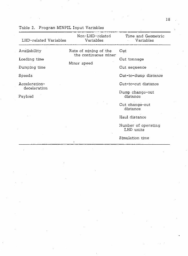
Table 2. Program MINPIL Input Variables
18
LHD-related VariablesNon-LHD-related
VariablesTime and Geometric
Variables
Availability
Loading time
Dumping time
Speeds
Acceleration-deceleration
Payload
Rate of mining of the the continuous miner
Miner speed
Cut
Cut tonnage
Cut sequence
Cut-to-dump distance
Cut-to-cut distance
Dump change-out distance
Cut change-out distance
Haul distance
Number of operating LHD units
Simulation time

19
distance from the dumping point and its distance from the center of mass
of the next cut in sequence.
Cut Tonnage. The cut tonnage is the mass of material contained
in the cut. It should be pointed out that this variable is adequate to
define the geometrical volume of the cut. Consequently, the dimensions
of the cuts are not needed as input to the program. They are only
needed to define the mass of the cut. Cut tonnage is treated determinis-
tically as input to the program.
Cut Sequence. Cut sequence defines the mining sequence of the
cuts and is of major importance to the program. Its importance is based
on the fact that it is the only variable with which the mine plan of a
specific operation can be simulated. Figures 2, 3, and 4 attempt to show
the importance of the cut sequence for the program.
Figure 2 illustrates a typical room-and-pillar panel. It is easily
understood that the choice of the appropriate cut tonnage (defined by its
dimensions) and sequence can result in the formation and'simulation of
rooms and pillars of the desired size, which is one of the mine plan objec
tives. Figure 3 shows that the correct choice of cut tonnage and sequence
can simulate a typical adit development. Figure 4 illustrates the simula
tion case where LHD units do not operate in the face but are used to haul
a pile of ore.

20
29 39 2822
Ai : LOADING AREA
A - i : CUT CHANGE-OUT DISTANCE
P : DUMP CHANGE-OUT DISTANCEE ,D i HAUL DISTANCEFULL-PUSH T R IP : A - B - E - P - B - A
CIRCULAR T R IP : A - B - E - F - D - B - A
DP: DUMPING POINT
Figure 2. Basic param eters for a typical room-and-pillar panel

21
GUI *3
CUT #2
CUT rLF
LP LHD LOADING POINT
DP : LHD DUMPING POINT
L P -D P ; LHD TRIP
DP
Figure 3. Sequence of cu ts with which program MINPIL can simulate a typical adit development

22
c t : t #1
CUT #2
CUT
L ? : LHD LOADING POINT
DP : LHD DUMPING POINT
L F-D P : LHD TRIP
DP
Figure 4. Sequence of cuts with which program MINPIL can simulate a typical pile removal

23
Output
The program output is divided into a production summary, a
haulage summary, and a wait-time analysis. Table 3 summarizes the
program output.
Table 3. Program MINPIL Output
Production Summary Haulage Summary Wait-Time Analysis
Tons delivered to Average LED cycle LED working timedump time
Machine-minutes Standard deviation of LED wait timesimulated LED cycle time
Production rate in Production rate in LED downtimetons per minute kilometer-tons
per minute
Production rate in LED utilizatontons per machine-minute
Simulation Procedure
The simulation procedure of program MINPIL is based on the
operation of a circular queue. Before giving details about the procedure
some general definitions are presented.
Definitions.
1. A queue is an ordered list in which all insertions take place at
one end, the tail, and all deletions take place at the other end, the front.
A queue is represented by means of an array Q (l:n ).
24
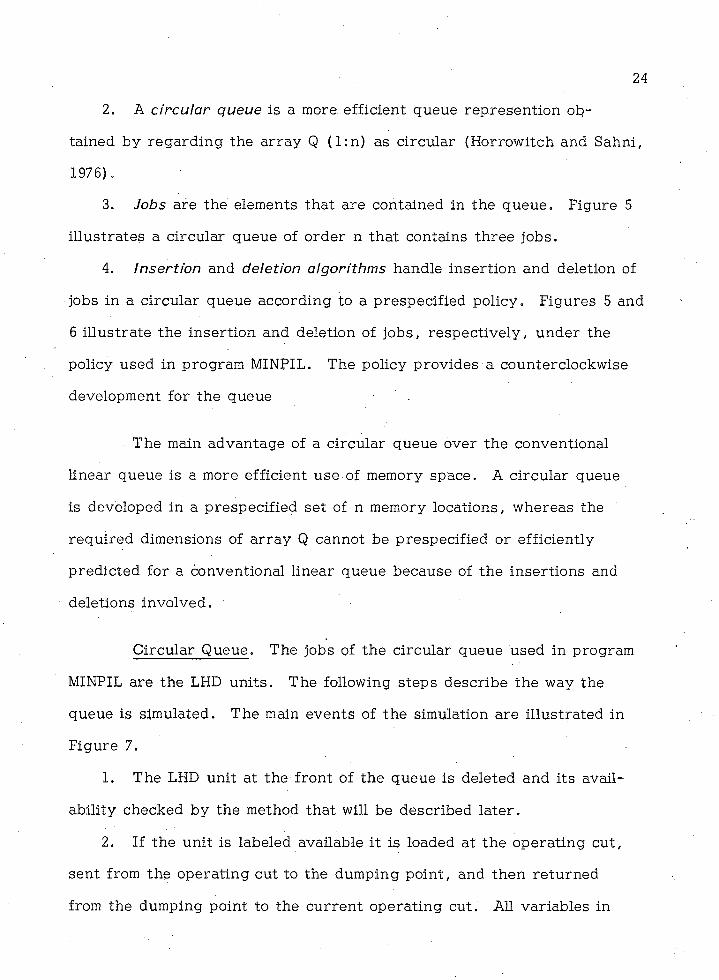
2. A circular queue is a more efficient queue represention ob
tained by regarding the array Q (l:n ) as circular (Horrowitch and Sahni,
1976).
3. Jobs are the elements that are contained in the queue. Figure 5
illustrates a circular queue of order n that contains three jobs.
4. Insertion and deletion algorithms handle insertion and deletion of
jobs in a circular queue according to a prespecified policy. Figures 5 and
6 illustrate the insertion and deletion of jobs, respectively, under the
policy used in program MINPIL. The policy provides a counterclockwise
development for the queue
The main advantage of a circular queue over the conventional
linear queue is a more efficient use of memory space. A circular queue
is developed in a prespecified set of n memory locations, whereas the
required dimensions of array Q cannot be prespecified or efficiently
predicted for a conventional linear queue because of the insertions and
deletions involved.
Circular Queue. The jobs of the circular queue used in program
MINPIL are the LED units. The following steps describe the way the
queue is simulated. The main events of the simulation are illustrated in
Figure 7.
1. The LED unit at the front of the queue is deleted and its avail
ability checked by the method that will be described later.
2. If the unit is labeled available it is loaded at the operating cut,
sent from the operating cut to the dumping point, and then returned
from the dumping point to the current operating cut. All variables in
25
FRONT
(a)
TAIL
FRONT 'AIL
Figure 5. Insertion of job D in the circular queue
(a)
FRONT TAILTAIL
FRONT
Figure 6. Deletion of job A in the circular queue

START
RECORD TIME UNIT WAS CALLED
PLACE UNIT AT END OF QUEUE
CALL FIRST UNIT OF QUEUE
ISNIT AVAILABLE
WASUNIT AVAILIAB
LAST TIME
COMPUTEDOWNTIME
LHD IS LOADED
LHD GOES TO DUMPAND
RETURNS TO CUT
COMPUTE DELAYS
DUE TO MINER
COMPUTE POSSIBLE
QUEUEING TIME
IS SHIFT OVER
NO
PLACE UNITAT END OF QUEUE
Figure 7, Main events of the program MINPIL circular queue

27
the program that simulates the trip are updated. When the unit returns
to the operating cut, it is inserted at the tail of the queue.
3. If the unit is labeled unavailable, it is inserted directly at the end
of the queue. The critical event in the circular queue operations is the
time the unit is checked for availability. This control takes place before
the unit is to be loaded.
Trip Time. A typical LHD trip comprises four activities: loading,
tramming, dumping, and queueing, which program MINPIL simulates. The
time for these four activities are calculated in the following manner.
1. Loading time. After the LHD has been labeled available, the unit
proceeds to the loading area and is loaded in time LT. The loading oper
ation may start at once when the unit enters the cut or it may be delayed
due to the performance of the miner. Program MINPIL determines and
records the delay time (DEL).
2. Tramming time. After being loaded, the unit trams to the dump
ing point and then returns to the operating cut. Program MINPIL calcu
lates tramming time using average values as follows:
Let TOTIME = tramming time
ACR = acceleration
BRR = braking rate
DIS (I) = distance between cut I and dump
LL(I) = cut change-out distance for cut I
LD (I) = dump change-out distance for cut I
SDUMP = average speed for dump change-out
28
SCUT = average speed for cut change-out
SHAUL = average speed for haul
The time for the LHD unit to travel from cut to dump (T) is the sum of the
cut change-out time ( T l ) , haul time (T 2), and dump change-out time
(T3), or
T = T l + T2 + T3
where: Tl = f(SCUT, ACR, LL(I))
T2 = f(SHAUL, SCUT, ACR, DIS(I), LL(I), LD(I))
T3 = f(SHAUL, SDUMP, BRR, LD(I))
The total tramming time for a trip would be:
TOTIME = 2 T
3. Dumping time. The time required for an LHD unit to dump its
load at the dumping point is the dumping time (DT).
4. Queueing time due to no passing policy. If an LHD is delayed in
the queue because of the no-passing policy, this time (TQ) is recorded
by program MINPIL.
The total time required for an LHD unit to complete a round trip
is:
Total Trip Time = LT + DEL + TOTIME + DT + TQ
Miner Activity. If a continuous miner is incorporated in the
mining operation, program MINPIL performs the following tasks:

29
1. Determines if the miner has excavated enough material at the
time the available LHD unit is ready for loading. If the material is ade
quate the unit is loaded. If not, the time the unit has to wait for the
material to be excavated (PQ) is recorded.
2. Determines if the loading area is occupied by another unit. If it
is not occupied, the program performs step 1. If it is occupied, the
program forces the unit to wait until the area is free, records the time
the unit must wait until the other unit is loaded (SQ), and then performs
step 1.
3. Calculates the time the unit has to wait in the loading area before
loading activities begin (DEL) as
DEL = PQ + SQ
and records DEL.
Queueing Time Due to No-passing Policy. A delay in the LHD
trip caused by the no-passing policy is examined and recorded by the
program. This delay time (TQ) is found by comparing the arrival time in
the loading area for the unit under consideration (TARIV) with arrival
time of the last unit called and found available before the arrival of the
Unit under consideration (T'ARIV).
If TARIV >T'ARIV, TQ = 0.
If TARIV < T'ARIV, TQ f 0 = T'ARIV - TARIV
Mechanical Availability. The mechanical availability of an LHD
unit is used by the program as a breakdown generator, that is , a task
that defines if the particular unit is available when it is called.

30
The task of labeling an LHD unit available or unavailable is performed by
a randomizing method, which works according to the following steps:
1. A random decimal number RN is called.
2. It is specified that RN be smaller or larger than AV.
3. If RN _< AV, the unit is labeled available; if RN > AV, the unit
is labeled unavailable. Figure 8 illustrates the method and gives two
examples.
LHD Downtime. The time a particular unit is down (DW) is re
corded by the program. The steps with which the program works are:
1. The time LHD unit I is called and found unavailable (CLN(I)) is
recorded.
2. The time LHD unit I is called again and found available (DCL) is
also recorded.
3. The program calculates total downtime for unit I as:
DW = (DCL - CLN(I))
Simulation Philosophy. The simulation philosophy used in pro
gram MINPIL is event oriented; that is , the state of the system remains
constant until the next event is reached (Kim, 1875). In this program
the events occur whenever one of the following conditions are met:
1. The LHD is called and found unavailable.
2. The LHD is called and found available.
3. The LHD loading is completed.
4. The LHD returns to the operating cut.
5. The LHD is ready for loading.
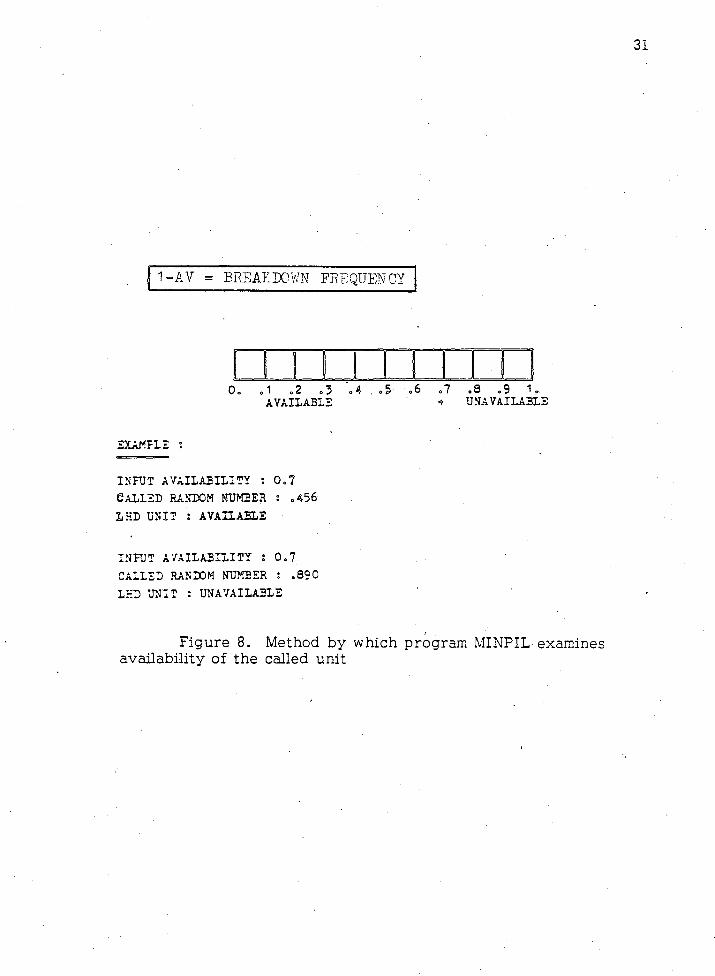
1-AV = BREAKDOWN FREQUENCY
M M I I I I T T !0. „1 .2 .3 o4 . .5- .6 .7 .8 .9 1.
AVAILABLE «• UNAVAILABLE
EXAMPLE :
INPUT AVA ILABILITY : 0 . 7
c a l l e d random n u m b e r : .4 5 6
LKD UNIT s AVAILABLE
INPUT A V A ILABILITY : 0 . 7
CALLED RANDOM NUMBER : .8 9 0
LHD UNIT : UNAVAILABLE
Figure 8. Method by which program MINPIL examines availability of the called unit
32
Program Capabilities
Deterministic Simulation
The program is capable of performing deterministic simulation by-
using multiple runs and changing the value of a specific variable to be
studied. The variables that can be changed are LHD availability, con
tinuous miner availability , distance between the first cut in the sequence
and the dumping point, average LHD haul speed, LHD heaped capacity,
and cut tonnage. The results of the multiple runs are output by program
MINPIL as horizontal histograms that show the impact of the changes of
the particular variable on the production recorded at the dumping point.
Range of Variables-
Under present dimensioning of the variables, the program can
handle no more than 10 LHD units working at the same face and no more
than 60 cuts in a mining cycle.
Assumptions Used in the Model
Certain assumptions incorporated in the model development may
affect the accuracy of the program. However, they do not impose serious
limitations on program application. The most important assumptions are:
1. All LHD units discharge at the same point, which is considered
the dumping point for the simulation area.
2. To define the exact values of the characteristics of an LHD trip
(loading and dumping times, change-out and haul speeds, heaped capac
ity) , the Monte Carlo sampling method is used in conjunction with input
normal distributions of the above characteristics. The normal
k

33
distributions of the above characteristics provide the sample values that
are used as average values to simulate the particular LHD trip.
3. Change-out distances for a particular cut are the same for all
opearating LHD units.
4. The distance from a particular cut to the dumping point is the
same for all LHD units.
5. A small tonnage of ore can be stored for a time at the face.
6. All the mass of a cut is concentrated at its center of mass
7. All recorded distances are measured from the center lines of the
covered drifts and cross cuts.
8. The program cannot handle LHD dispatching; that is , the pro
gram needs a prespecified number of LHD units assigned to the working
miner or the working face of the simulated area.
9. If pull-push LHD trips are incorporated in the program, queue
ing time is not recorded because of the no-passing policy. The reason
for that assumption is that in a pull-push trip environment, each LHD
has its own route from the cut to the dumping point and queueing time
in the drifts therefore does not exist.
10. In the conventional mining method option of the program, where
a continuous miner is not used, loading and tramming operations take
place continuously and cannot be interrupted by any other face operation.
11. Both in the conventional and continuous methods, the mine bolter
or any other support unit is outside the boundaries of the simulation.
12. The program uses the concept of availability as a breakdown
generator.

fVALIDATION OF PROGRAM MINPIL
This chapter deals with the validation of program MINPIL with
artificial test data for the application of LHD equipment in four different
cases where the room-and-pillar methods is used. The first case studies
the effect of queueing times due to LHD trips. The program was run with
different number of LHD units performing circular trips. The resulting
queueing times were recorded and studied. The second case illustrates
the effect of the use of a continuous miner on productivity of LHD units.
For comparison, the program was run using the same data as in the first
case with the additional element of a continuous miner. The third case is
a joint sensitivity analysis of the effect of haul distance and number of
LHD units on LHD productivity. The program was run for different num
ber of units and a different haul distance each time. The last case was
the simulation of LHD operation in an actual room-and-pillar panel. For
this case the program was run four times and the individual LHD statistics
recorded and studied.
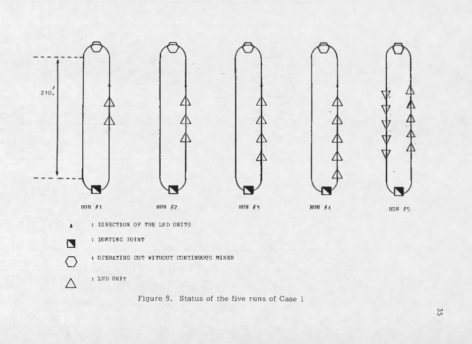
Case 1: To study the effect of trip queueing time on LHD pro
ductivity, program MINPIL was run five times. The first run used 2 LHD
units, the second 3 units, the third 4 units, the fourth 5 units, and the
fifth 10 units. Figure 9 illustrates the status of the circular trip of each
run. In this case study, the following input data were used:
LHD availability 70%
LHD average haul speed: 330 ft/min; SD = 0
34
RUN ^1
z x
zOx
z xz xz x
RUN n
4 : DIRECTION OF THE LHD UNITS
: DUMPING IOINT□O
A
ZXZXZXZX
RUN
: OPERATING CUT WITHOUT CONTINUOUS MINER
: LHD UNIT
RUN #/| RUN #5
Figure 9. Status of the five runs of Case 1u>cn
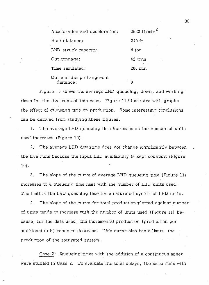
2Acceleration and deceleration: 3620 ft/min
Haul distance.: 210 ft
LHD struck capacity: 4 ton
Cut tonnage: 42 tons
Time simulated: 200 min
Cut and dump change-outdistance: 0
Figure 10 shows the average LHD queueing, down, and working
times for the five runs of this case. Figure 11 illustrates with graphs
the effect of queueing time on production. Some interesting conclusions
can be derived from studying.these figures.
1. The average LHD queueing time increases as the number of units
used increases (Figure 10).
2. The average LHD downtime does not change significantly between
the five runs because the input LHD availability is kept constant (Figure
10) .
3. The slope of the curve of average LHD queueing time (Figure 11)
increases to. a queueing time limit with the number of LHD units used.
The limit is the LHD queueing time for a saturated system of LHD units.
4. The slope of the curve for total production plotted against number
of units tends to increase with the number of units used (Figure 11) be
cause, for the data used, the incremental production (production per
additional unit) tends to decrease. This curve also has a limit: the
production of the saturated system.
Case 2: -Queueing times with the addition of a continuous miner
were studied in Case 2. To evaluate the total delays, the same runs with

109
89
J ,“ 1RUN #1 RUN //2
Q : QUEUEING TIME D: TOWN TIME
RUN
W: WORKING TIME
8 9 W
-
9 2
18
RUN #4 RUN #5
.1 5 0
D JL 100 m in .
50
Figure 10. Average LHD queueing, down, and waiting times for the five runs of Case 1
GO

5 10 15 2 0 25 30 35 40 45 4 0 0 5 0 0 6 0 0 7 0 0 8 0 0
AVERAGE LHD QUEUEING TIMETOTAL PRODUCTION IN TONS
IN MINUTES
Figure 11. Results of Case 1 COCO

39
the same characteristics as in Case 1 were made. The only additional
element introduced was the incorporation of a continuous miner with the
following characteristics:
Miner availability: . 50%
Mining rate: 8 ton/min
Tramming speed: 120 ft/min
Figure 12 presents the status of the five runs of this case
Figure 13 shows the average LHD queueing, down, and working times
for each run, and Figure 14 illustrates with curves the effect of the new
queueing times (due to LHD trips and continuous miner) on productivity.
All conclusions of Case 1 can be derived from this study. Addi
tional conclusions are:
1. The curves in Figure 14 for Case 2 and those in Figure 11 for
Case 1 were constructed in a similar fashion to permit comparison. Be
cause the only element that was changed in Case 2 was the incorporation
of a continuous miner, any difference between the curves must be attrib
uted to the miner.
2. The average LHD queueing time (Figure 13) increases faster as
the number of units used increases. The queueing time now is the sum
of the delays from Case 1 and the new delays imposed by the continuous
miner.
Case 3: The third case performs a joint sensitivity analysis for
the effect of number of LHD units and average haul distance on produc
tivity. The program was run four times, changing the two elements as
follows:

2 1 0 .
□0A
RUN it'i RUN
: DIRECTION. OF THE LHD UNITS
: DUMPING POINT
: OPERATING CUT WITH CONTINUOUS MINER
: LHD UNIT
RUN RUN H
Z 0 \
VVVVV
AAAAA
RUN ff'i
Figure 12. Status of the five runs of Case 2iCho

56
103 W 9 7 W 9 3 w 81 W
102
94 D 91 D 91 D 97 D
42
11 Q Q II . 21* Q6 2
RUN #1 RUN #2 RUN # 3 RUN #4 RUN #5
Q : QUEUEING TIME D :‘ DOWN TIME W; WORKING TIME
Figure 13. Average LHD queueing, down, and waiting times for the five runs of

NUM
BER
OF
LHD
UN
ITS
10
9
8
7
6
5
4
3
2
1
4 0 0 5 0 0 6 0 0 7 0 0 8 0 0 9 0 030 35 40 45 5010 1 20
AVERAGE LHD QUEUEINGTOTAL PRODUCTION IN TONS
TIME IN MINUTES
_____________ I SIMILAR GRAPH OF THE CASE I
Figure 14. Results of Case 2

43
Average HaulRun Number of LHDs Distance (ft)
1 2 200
2 3 300
3 4 600
4 1 800
The status of the four runs is shown in Figure 14. The remain
ing input data used in this case were:
. LHD availability 70%
LHD struck capacity: 4 tons
Haul speed: 330 ft/min
Continuous miner rate: 5 tons
Continuous miner availability: 50%
Cut and change-out distance: 0
Time simulated: 200
Figure 16 illustrates the effect of haul distance and number of
LHDs used on production. From this figure the following conclusion is
derived. The production when the program was run with two units and
a 200-foot haul distance or three units and a 400-foot distance or four
units and a 600-foot distance is 360 to 385 tons. This finding shows that
the extra advantage introduced by incorporating an additional LHD unit
is approximately canceled by the increase in haul distance. If the rate of
increase in haul distance is proportionately the same as the rate of in
crease in number of LHD units (1:2:2 = 200:400:600), productivity is
apparently equally sensitive to both variables within the range used in
this case.

z ^ x Z ^ X / ^ x z ^ x
200 .
A
A 4 0 0 .
A6 0 0 . '
A
RUN
RUN if 2
k
H
QA
AA
RUN
: DIRECTION OF THE LHD UNITS
: DUMPING POINT
: OPERATING CUT WITH CONTINUOUS MINER
: LHD UNIT
A8 0 0 .
RUN
Figure 15. Status of the five runs of Case 3 0

400
300TOTAL PRODUCTION
IN TONS200
100NUMBER OF LHD
UNITS
200HAUL DISTANCE
6 0 0
800
Figure 16. Three-dimensional diagram showing the results of joint sensitivity analysis4cn

46
Case 4: The fourth case is the simulation of an actual room-and-
pillar panel (Figure 17). The program was run with 2, 3, 4, and 10 LHD
units. The output data for each of the four runs are presented in Table
4. Input data for Case 4 were:
Cut change-out distance: 30 ft
Dump change-out distance: 30 ft
Number of cuts simulated: 30
LHD availability: 80%
Average LHD haul speed: 440 ft/min; SD = 10
LHD cut and dumpchange-out speed: 350 ft/min; SD = 10
LHD loading and dumping time: 0.5 min; SD = .05
LHD heaped capacity : 7 ton
Acceleration and deceleration: 3520 ft/min2
Time simulated: 500 min
Studying the results shown in Table 4 permits derivation of
several conclusions:
1. Working times are different fori the individual LHD units. This
is an effect of (a) the randomized method used by the program to deter
mine the availability of a unit and (b) the different Speeds andloading
and dumping times generated randomly from the input distributions for
each LHD trip.
2. Again, because input LHD availability does not change, the LHD
downtimes do not differ appreciably.
3. The productions (load hauled. Table 4) decrease for individual
units because LHD waiting time increases with introduction of more units.

47
10
10' t
5 0 0 '
1 0 0 '30 29
28 27 26 2 5
24 2 3 22 21
2 0 19 18 .-7
16 15 14 13
12 11 10 9
8 7 6 5
4 3 2 1
j j j DUMPING PO IN T
. CUT CHANGE-CUTDUMP CHANGE-OUT
HAITI DISTANCE
Figure 17. Room-and-pillar panel used for Case 4
*
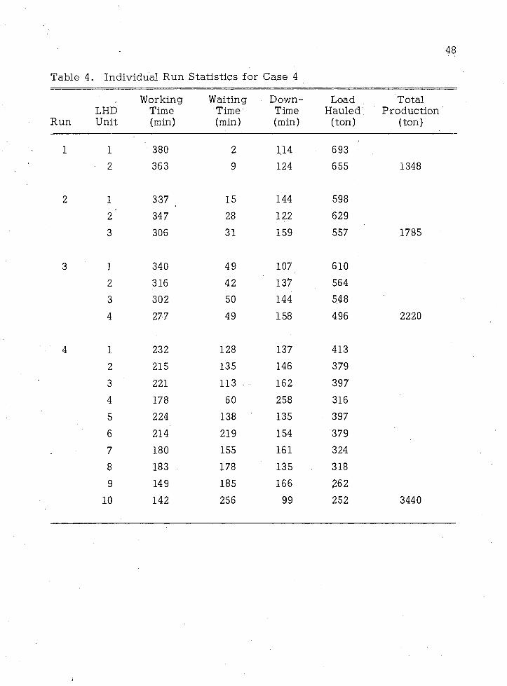
Table 4. Individual Run Statistics for Case 4
48
RunLHDUnit
WorkingTime(min)
WaitingTime(min)
Down-Time(min)
LoadHauled
(ton)
TotalProduction
(ton)
1 1 380 2 114 6932 363 9 124 655 1348
2 1 337 _ 15 144 5982' 347 28 122 6293 306 31 159 557 1785
3 . 1 340 49 107 6102 316 42 137 5643 302 50 144 5484 277 49 158 496 2220
4 1 232 128 137 4132 215 135 146 3793 221 113 162 3974 178 60 258 3165 224 138 135 3976 214 219 154 3797 180 155 161 3248 183 178 135 3189 149 185 166 262
10 142 256 99 252 3440
APPLICATION OF PROGRAM MINPIL
Program MINPIL was used to simulate the performance of LED
units at'.five coal mines operated by the same company. The steps in the
simulation study were to adjust the model structure for the particular
operating environment at each mine and to apply the adjusted simulation
model to the specific problem of evaluating the performance of the LED
model used at that mine. The following sections discuss the adjustment
procedure and the results of the simulation.
Program Adjustment
The mining company had recently introduced LED equipment to
its operations and wished to evaluate the performance of the different
LED types working under almost identical operational conditions. The
five mines at which the simulation studies were conducted provided the
standard conditions needed for equipment comparisons because they all
use the room-and-pillar mining method and have almost the same face
characteristics. The company provided all the required input data for
each mine and LED type. A great deal of the needed data (working time,
normal delay time, loading and dumping times, net tonnages, production
per shift) were in the form required by the program. The remaining
data (acceleration and braking rate, average trip speed, average LED
load) were computed from available time studies.
With all operational data available, the adjustment could be
focused on the selection of an availability figure for each unit at each
49

50
mine. This determination was necessary because the initial time studies
did not include abnormal delay times and the simulation model is highly
dependent on this variable. A number of runs were performed using
different availabilities for each LHD type to determine the availability
values that produced the best match between actual and computed pro
duction per shift.
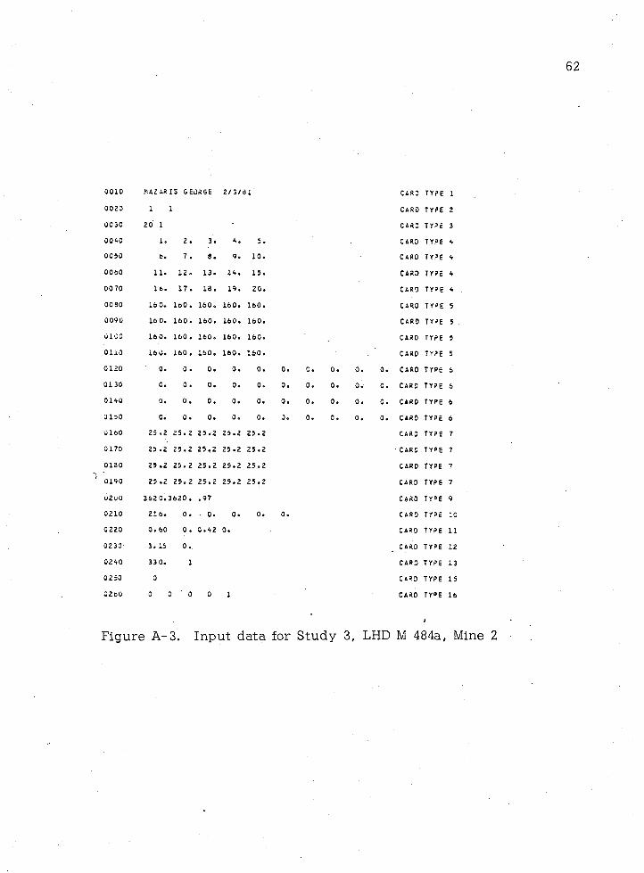
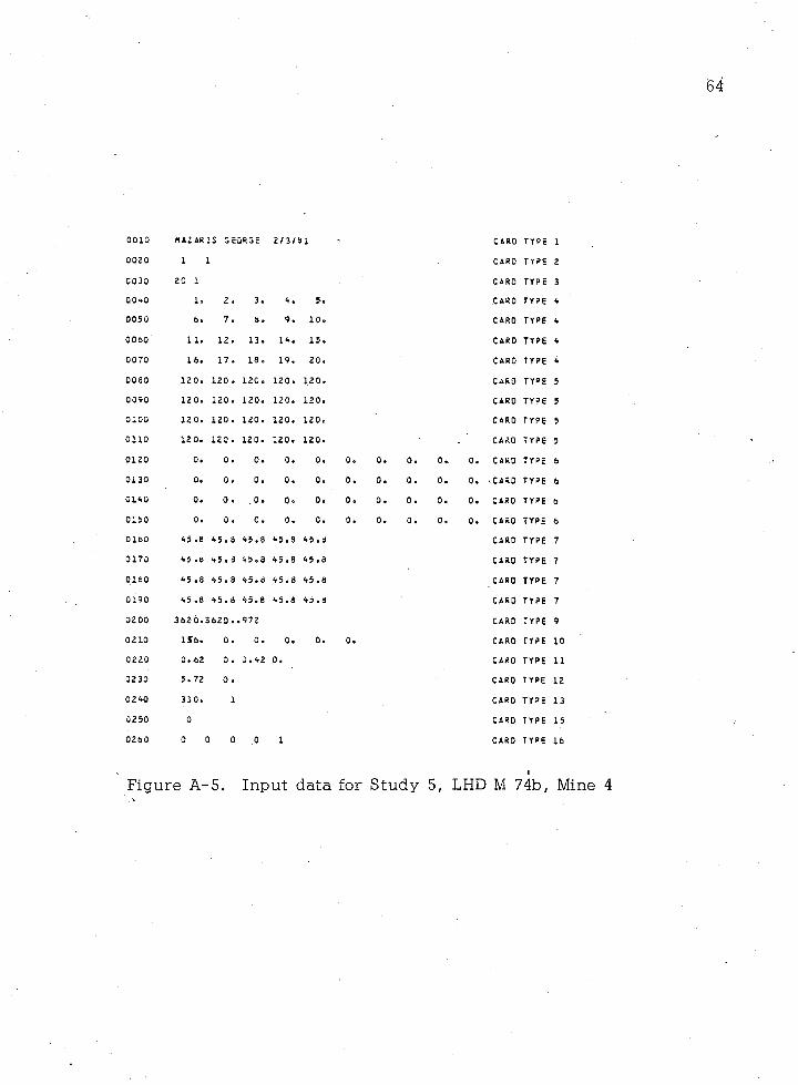
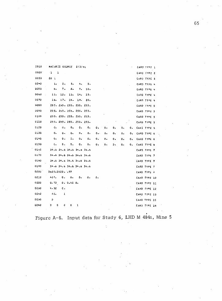
Table 5 summarizes the input data used in the simulation studies
of the various LHD units. Figures A -l through A -6 (Appendix A) pre
sent the same input data in the format required by program MINPIL.
Table 6 gives a summary of the program outputs for the six simulation
studies. The actual program outputs for each LHD unit are given in
Figures A-7 through A -12 (Appendix A) . Note that six simulation studies
were required to study the five models because at one mine (Mine 2)
Model 484a was operated at two cut-dump distances.
The output data presented in Table 6 permit the following con
clusions :
1. The range of availability values that best fit the various runs is
97-100 percent, a result that was expected because the time used for the
studies was one shift and the input data for each LHD unit (with one ex
ception) derived from successful sh ifts , i . e . , with no abnormal delays.
2. In general, the model fits the actual situation. The differences
between actual and computed productions per shift have a range from -6 1 ,
to +4 percent with a mean deviation of -4 percent.

Table 5:„ Summary of Input Data for Operational LHD Units
Acceleration and deceleration = 3620 ft/min^
LHDModel
#Study Mine
#
HeapedCapacity
(tn)
StudyTime(min)
CutTonnage
(tn)
Cut-DumpDistance
(ft)
Availability
(%)
Average Speed
(ft/min)
LoadingTime(min)
DumpingTime(min)
M 480 1 1 4 330 41.8 210 97 334 0.69 0.42
M 480a 2 2 3.15 330 25.2 280 97 216 0.60 0.42
3 2 3.15 330 25.3 160 97 216 0.60 0.42
M 74a 4 3 2.65 330 29.2 280 100 241 0.37 0.34
M 74b 5 4 5.72 330 45.8 120 97.2 156 0.62 0.42
M 484b 6 . 5 4.32 92 34.6 255 100 407 0.73 0.42
cn

Table 6. Summary of Productivities and Rankings of LHD Models
Numbers in parenthesis are rankings of LHD models by study
LHDModel
#Study
#Mine
#
Productivity
tn / shift
tn /minModelRank tn/Mmina
ModelRank km-tn/min
ModelRank. Actual
Computed Diff.
ModelRank
M 480 1 1 575 (2) 572 (2) -1% 2 1.73 (.3) 3 1.87 (3) 3 32 (1) 1
M 484a 2 2 287 (5) 299 (5) +4% 0.90 (6) 0. 95 (5) 15 (5) ■
3 2 420 (3) 434 (3) +3% 1.31 (4) 1.43 (4) 18 (4)
354b 367b 3 I.IQ5 4 1 .12b 4 16b 4
M 74a 4 3 330 (4) 310 (4) -6% 4 0.94 (5) 5 0.94 (6) 5 19 (3) 3
M 74b 5 4 733 (1) 720 (1) -2% 1 2.18 (1) 1 2.32 (1) 1 20 (2) 2
M 484b 6 5 190 (6) 177 (6) -6% 5 1.92 ( 2) 2 1.95 ( 2) 2 12 (6) 5
a. Mmin = time (minutes) LHD unit, is in motion.b. Average for the two M 484a units.
Results of Program Application
When the model had been adjusted to the existing operation, it
was used to obtain an estimation of the productivity for each LHD model
studied and to perform a sensitivity analysis for the average LHD haul
speed for each LHD model.
Productivity Estimation
The main objective for the company's introducing different LHD
models was to examine the behavior of each model and to derive conclu
sions about its operation for future applications. Consequently, program
MINPIL was used to measure the performance of each LHD model and to
compare the productivities of the various models. The output summary
(Table 6) gives four measures of productivity that can be used for quan
titative comparisons of performance:
1. LHD productivity in tons' per shift.
2. LHD productivity in tons per minute.
3. LHD productivity in tons per machine-minute.
4. LHD productivity in kilometer-tons per minute.
Shift production is not a representative comparison figure becausei
it does not consider the differences between mines. Note that the study
time for Model 484b (study 6) was only 92 minutes because of mine condi
tions. Also note the different ranks obtained for the two Model 484a units
operating at mine 2 (studibs 2 and 3) where each model operated at a dif
ferent cut-dump distance.
Productivity measured in either tons per minute or tons per
machine-minute does not incorporate differences in trip distances and is
54
therefore not a reliable comparison figure for a study in which trips
differ (Table 5). Again observe the differences in ranking for the two
Model 484a units.
Because the LHD models have different characteristics (average
speeds) and operate over different trip distances, the performance cri
terion to be used must take into account all operating differences to give
an unbiased result. The output variable that best fits a complex compari
son is productivity measured in kilometer-tons per machine minute. In
this study the availabilities used were high (97%-100%), therefore the
introduction of machine-minutes in this measurement of productivity would
not improve the comparison.
Table 5 also gives the ranks of the five LHD models being judged
by the four output measures for productivity. It is evident that the
ranks as determined by prqducitivity in kilometer-tons per minute do not
coincide with either the ranks for tons per shift or for tons per minute
or tons per machine-minute. Some interesting points concerning the
various results can be pointed out.
The most productive unit as measured in kilometer-tons per
minute is LHD M 480 working in mine 1. This unit ranked third in
productivity by the other three productivity measures. In contrast,
LHD M 74b working in mine 4 ranked first for productivity measured in
tons per shift, tons per minute and tons per machine-minute but ranked
second to LHD M 480 in kilometer-tons per minute. It is interesting to note
that although LHD 74b had the largest heaped capacity of the five models
studied, it had the lowest average speed. It is clear that if the method
55
for determining productivity had not incorporated kilometer-tons, the
difference in productivity would not have been evident.
Analysis of Sensitivity of Productivity ■ to Average Haul Speed
Having defined the performance of all LHD models, a sensitivity
analysis was made of the effect Of average haul speed on productivity
measured as tons per shift. The reason for choosing average haul speed
as the variable to study was that it best reflects actual working conditions
in the mines. Improvement or deterioration of LHD operation due to use
of tire chains, increase or decrease in trip delays, or better or worse
ground control will have an immediate impact on average LHD speed and
will influence shift production.
Figures B-7 through B-12 illustrate with horizontal histograms
generated by the program the results of the sensitivity analysis. The
required input data for the various sensitivity analyses are also presented
in Appendix B. Such histograms can help the user define the new pro
duction figure when haul speed is changed.

CONCLUSIONS
Capability of Program MINPIL to Handle Varied Operating Characteristics
Program MINPIL can solve a variety of problems in the operation
of LED units. These problems can be divided into two categories: (1)
problems concerning room-and-pillar mining methods and (2) problems
arising in general applications of LED equipment. Some specific examples
follow.
Room-and-Pillar Mine Layout Problems
For a specific set of equipment it is often desired to find the
optimum cut sequence and cut dimensions for a particular room-and-pillar
panel. By using the multiple-runs option of the program and changing
the cut dimensions or cut sequence for each run, program MINPIL can
determine the optimum layout.
Another problem may be to determine the optimum set of equipment
to work in a prespecified panel. Again, by using the multiple-runs op
tion and changing the number or characteristics of the LED units in the
set or the characteristics of the miner for each run, program MINPIL can
provide information for the optimum equipment selection. It is also pos
sible to simulate the current panel layout for the current set of equipment
by incorporation the first option of the multiple-runs option. This pro
gram capability was tested in the study by simulating the present situ
ation in equipment and panel geometry for the six LED operations.
56

57
The program is also capable of performing sensitivity analyses by
changing one variable in a set of variables during each run by using the
multiple-runs option. The program displays the results of the analysis
as histograms. The sensitivity capability of program MINPIL was demon
strated in this study by analyzing the sensitivity of LHD productivity to
average haul speed.
Program MINPIL is also able to handle circular or pull-push LHD
trips in a room-and-pillar panel and the operation of LHD units in room-
and-pillar mining with continuous miners or the conventional mine cycle.
General LHD Applications
Program MINPIL is able to simulate LHD operation in tunnel de
velopment work. The development work is treated as a special case of a
room-and-pillar procedure in which the cuts to be mined form the shape
of the tunnel. Several mining methods require the LHD units to load and
haul material from a loading point that is not in the face to another point.
By considering the material concentrated at the loading point as a mining
cut, the program is able to handle this operation. A similar problem is
the removal of a pile of material to another point or to a draw point.
This problem can be treated in the same way. ■ *
Suggested Refinements
Two refinements of program MINPIL are suggested. The first is
the incorporation of a detailed cycle time. Although high accuracy in
estimating the travel time of LHD trips is not required to simulate an
underground operation, it is suggested that a more accurate determination
58
of trip time might be achieved by incorporating the University of Arizona
program CYCLE (Kim and Dixon, 1977) into program MINPIL. Program
CYCLE accurately computes the trip time for any moving unit in a pre
specified or generated mine layout by using the characteristic rimpull
curve.
The second suggestion is that new modules be introduced into
the program to increase the number of problems that can be solved. Two
modules of special interest are one that would incorporate delays due to
operation of the bolter (or other roof-support operation) and one that
would simulate multiple-face operations with-or without LED unit dis
patching. ,

APPENDIX A
PROGRAM MINPIL INPUT AND OUTPUT FOR SIMULATION
STUDY OF LED OPERATION IN FIVE COAL MINES
59

60
0010 HAZ ARIS GEORGE 2/3/81 CARD TYPE 10020 1 1 CARD TYPE 20030 20 1 CARD TYPE 30040 1« 2 • 3. 4 o 5. CARD t y p e 40050 6. 7. 8. 9. 10. CARO TYPE 40060 11. 12. 13. 14. 15. CARD TYPE 40070 16. 17 o 18. 19. 20. CARD TYPE 40080 210. 210. 210. 210. 210. CARD TYPE 50090 210. 210. 210. 210. 210. CARD TYPE 50100 210. 210. 210, 210. 210. CARO TYPE 50110 210. 210. 210. 210. 210. CARD TYPE 50120 0. 0 . 0. 0. 0. 0. 0. 0. 0. 0. CARD TYPE 60130 0. 0 . . o. 0. 0. 0. 0. 0. 0. 0. CARD TYPE 60140 0. 0 . 0. 0. 0. 0. 0. 0. 0. 0. CARD TYPE 60150 0. 0. 0. 0. 0. 0. 0. 0. 0. 0. CARD TYPE 60160 41 .8 41.8 41.8 41.3 41 .8 CARD TYPE 70170 41.8 41, 8 41.8 41.d 41.8 CARD TYPE 70180 41.8 41,8 41.8 41.8 41.8 CARD TYPE 70190 41 .8 41. 8 41.8 41.8 41.3 CARD TYPE 70200 362 0. 3620 • 0.97 CARD TYPE 90210 334. 0. 0. 0. 0. 0. CARD TYPE 100220 0.69 0 • 0.42 0. CARD TYPE 110230 4. 0. CARD TYPE 120240 330. 1 CARD TYPE 130250 0 CARD TYPE 150260 0 0 0 0 1 CARD TYPE 16
Figure A -l. Input data for Study 1, LHD M 480, Mine 1

61
0010 MAZAAIS GEOkOE 2/3/61 CARO TY>E 10020 1 1 CAPO TfJE 20030 20 1 CARO TYPE. 30040 1. 2 . 3. 4, 5. CARD TYPE 4'0050 6o 7. 8. 9. 10. CARD type 40060 . 1 1. 12 . 13. 14. 15. CARD TYPE 40070 1 Co 17 . 16. 19. 20. CARD TYPE 400 o0 230. 280 . 260. 290. 280. CARD TYPE 50090 23 0. 280 . 280. 290. 230. CARD TYPE 5Cl 00 280, 260 . 2o0. 260. 280. CARO TYRE 50110 290. 280. 280. 23 0. 280. CARD TYPE 50120 0. 0 . 0. 0. 0. 0. 0. 0. 0. 0. CARD T Y°£ 6C130 0. 0 . 0. 0. 0. 0. 0, 0. 0. 0. CARD TYPE 60140 0, 0. 0. 0. 0. 0. 0. 0. 0. 0. CARD TYPE 60150 0. 0 . 0. 0. 0. 0. c. Oo 0. 0. CARD t y p e 60160 25 .2 25.2 25.2 25.2 25.2 CARO TYPE 70170 25 .2 25.2 25.2 25.2 25.2 CARD TYPE 70190 25.2 25.2 25.2 25.2 25.2 CARD TYPE 70190 25 .2 25.2 25.2 25.2 25.2 CARD TYPE 702 00 3620, 2620. .97 CARD TYRE 90210 21 6. 0 . 0. 0. 0. 0. CARD TYRE 100220 0. c0 0 . 0.42 0. CARD TYRE 110230 3. 15 0. CARD TYPE 120 2 40 33 0. 1 CARD TYPE 1302 50 0 CARO TYPE 150260 0 0 0 0 1 CARD TYPE 16
Figure A -2. Input data for Study 2, LHD M 484a, Mine 2
0010 NAZAR IS GEORGE 2/3/81 CARD TYPE 10020 1 1 CARD t y p e 20030 2 0 1 - CARD TYPE 30040 1. 2 . 3. 4. 5. CARD TYPE 40050 t o 7. 8. 9. 10. CARD TYPE 40060 11. 12. 13. 14. 15. CARD TYPE 40070 16. 17. 18. 19. 20. CARD t y p e 40080 160. 160. 160. 160. 160. CARD TY»E 50090 16 0. 160. 160. 160. 160. CARD TYPE 5 .0100 160. 160. 160. 160. 160. CARD TYPE 50110 160. 160 . 160. 160. 160. CARD TYPE 50120 0. 0 . 0. 0. 0. 0. 0. 0. 0. 0. CARD TYPE 60130 0. 0. 0, 0. 0. 0. 0. 0, 0. 0. CARD TYPE 60140 0. 0. 0. 0. 0. 0. 0. 0. 0. 0. CARD TYPE 63150 0. 0. 0. 0. 0. 0. 0. 0. 0. 0. CARO TYPE 60160 25 .2 25. 2 25.2 25.2 25.2 CARD TYPE 70170 25 .2 25.2 25.2 25.2 25.2 CARD TYPE 70130 25 .2 25.2 25.2 25.2 25.2 CARD TYPE 70190 25 .2 25.2 25.2 25.2 25.2 CARD TYPE 70200 3620. 3620 . .97 CARD TYPE 90210 216. 0. ' 0. 0. 0. 0. CARD TYPE 100220 0. 60 0 . 0,42 0. CARD TYPE 110230 3. 15 o.„ CARD TYPE 120240 330. 1 CARD TYPE 130250 0 CARD TYPE 150260 0 0 0 0 1 CARD TYPE 16
Figure A -3. Input data for Study 3, LHD M 484a, Mine 2

63
0010 MAZAR1S GEORGE 2/3/ 81 CARD TYPE 1 .
0020 1 1 CARD TYPE 20030 20. 1 CARD TYPE 30040 lo 2 . 3. 4. 5. CARD TYPE 40050 6. 7. 6. 9. 10. CARD TYPE 40060 11. 12. 13. 14. 15. CARD TYPE 40070 16. 17. 18. 19. 20. CARD TYPE 40060 260. 280. 280. 280. 280. CARD TYPE 50090 2d 0. 260 . 260. 280. 280. CARD TYPE 501Q0 23 0. 280 . 280. 280. 280. CARD TYPE 50110 230. 260 . 280. 280. 280. CARD TYPE 50120 0. 0 . 0. 0. 0. 0. 0. 0. 0. 0. CARD TYPE 60130 0. 0. 0. 0. 0. 0. 0. 0. 0. 0. CARD TYPE 60140 0. 0. 0. 0. 0. 0. 0. 0. 0. 0. CARD TYPE 60150 0. 0 . 0. 0. 0. 0. 0. 0. 0. 0. CARD TYPE 60160 29 .2 29.2 29.2 29.2 29.2 CARD TYPE 70170 29 .2 29.2 29.2 29.2 29.2 CARD TYPE 70160 29 .2 29.2 29.2 29.2 29.2 - CARD TYPE 70190 29.2 29. 2 29.2 29.2 29.2 CARD TYPE 70200 3&2 0. 3620 . 1. CARD TYPE 90210 241. 0 . 0. 0. 0. 0, CARD TYPE 100220 0. 37 0 . 0.34 0. CARD TYPE 110230 2.65 0 . CARD TYPE 120240 330. 1 CARD TYPE 130250 0 CARD TYPE 150260 - 0 0 0 0 1 CARD TYPE 16
Figure A -4. Input data for Study 1, LHD M 74a, Mine 3
64
0010 MAZARIS GEORGE 2/3/61 CARD TYPE 10020 1 1 CARD TYPE 20030 20 1 CARD TYPE 30040 1. 2 . 3. 4. 5 o CARD TYPE 40050 6 a 7. 8. 9. 10. CARD TYPE 40060 11. 12. 13. 14. 15. CARD TYPE 40070 16. 17. 18. 19. 20. CARD TYPE 40080 12 0. 120 . 120. 120. 120. CARD TYPE 50090 120. 120. 120. 120. 120. CARD TYPE 50100 12 0. 120. 120. 120. 120. CARD TYPE 50110 120. 120. 120. 120. 120. CARO TYPE 50120 0. 0. 0. 0. 0. 0, 0. 0. 0.. 0. CARD TYPE 60130 0. 0 . 0, 0. 0. 0. 0. 0. 0. 0, nCARD TYPE 60140 0. 0 . .0. 0. 0. 0, 0. 0. 0. 0. CARD TYPE 60150 0. 0. 0. 0. 0. 0. 0. 0. 0. 0. CARD TYPE 60160 45 .8 45.6 45.8 45.8 45.3 CARD TYPE 70170 45 .6 45.8 45.8 45.8 45.8 CARD TYPE 70180 45 .8 45. 8 45.8 45.3 45.8 CARD TYPE 70190 45 .8 45.8 45.8 45.8 45.3 CARD TYPE 70200 3 62 0. 3620 ..972 CARD TYPE 90210 156. 0. 0 . 0. 0. 0. CARD TYPE 100220 0.62 0 . 0.42 0. CARD TYPE 110230 5.72 0 . CARD TYPE 120240 330. 1 CARD TYPE 130250 0 CARD TYPE 150260 0 0 0 0 1 CARD TYPE 16
Figure A-5. Input data for Study 5, LHD M 74b, Mine 4
65
0010 HAZARIS GE0020 1 . i0030 20 10040 1. 2.0050 6, 7.0060 11. 12.0070 16. 17.0080 255, 235 .0090 25 5. 255 .0100 255. 255.0110 25 5. 255 .0120 C. 0.0130 0. 0 .0140 0. 0 .0150 0. 0.0160 34,6 34,60170 34 .6 34.60180 34 .6 34, 60190 34 .6 34.60200 3620.:3620 .0210 407. 0 .0220 0. 73 0 .0230 4. 32 0 .0240 92. 10250 00260 0 1D 0
SE 2/3/dl
3. 4. 5.8. 9. 10.
13. 14. 15.13. 19. 20.
255. 255. 255.255. 255. 255,255. 255. 255.255 , 255. 255.
0. 0. 0.0. 0. 0.0. 0. 0.0. 0. 0.
34,6 34 . 6 34.634.6 34.6 34,634.6 34.6 34.634.6 34.6 34.6.97
0. 0. 0.0.42 0.
0 1
0. 1 0. 0. 0.0. 0. 0. 0.0. 0 o 0. 0.0• 0. Do o.
CARD T Y36 1CARD TYPE 2CARD TYPE 3CARD t y p e 4CARD t y p e 4CARD TYPE 4CARD TY3E 4CARD TYPE 5CARD TYPE 5CARO TY»E 5CARD TYPE 5
0. CARD TYPE 60. CARD TYPE 60. CARD TYPE 60. CARD TYPE 6
CARD TYPE 7CARO TYPE 7CARD TYPE 7CARD TYPE 7CARD TYPE 9CARD TYPE 10CARD TYPE 11CARD TYPE 12CARD TYPE 13CARD TYPE 15CARD TYPE 16
Figure A-6. Input data for Study 6, LHD M 484a, Mine 5
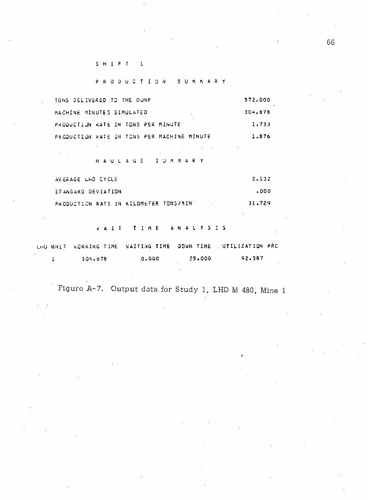
S H I F T 1
P R O D U C T I O N S U M M A R Y
TONS DELIVERED TO THE DUMP 5 7 2 . 0 0 0
MACHINE MINUTES SIMULATED , 3 0 4 . 8 7 8 .
PRODUCTION KATE IN TONS PER MINUTE 1 . 7 3 3
PRODUCTION KATE IN TONS PER MACHINE MINUTE 1 . 8 7 6
H A U L A G E S U M M A R Y
AVERAGE LHO CYCLE 2 . 1 3 2
STANDARD DEVIATION . 0 0 0
PRODUCTION RATE IN KILOMETER TONS/MIN 3 1 . 7 2 9
* A I T T I M E A N A L Y S I S
IhU U N IT UQRKING TIME WAITING TIME DOWN TIME UT I L I Z A T IO N PRC
1 3 0 4 . 8 7 8 0 . 0 0 0 2 5 . 0 0 0 9 2 . 3 8 7
Figure A -7. Output data for Study 1, LHD M 480, Mine 1

67
S H I F T i
P R O D U C T I O N S U M M A R Y
TONS' DEL IVtRED TO THE DUMP 2 9 9 . 2 5 0
MACHINE MINUTES SIMULATED 3 1 4 . 6 3 3 •
PRODUCTION RATE IN TONS PER MINUTE . 9 0 7
PRODUCTION RATE IN TONS PER MACHINE MINUTE .9 5 1
H A U L A G E S U M M A R Y
AJERAGE LHD CYCLE 3 . 3 1 2
STANDARD DEVIATION . 0 0 0
PRODUCTION RATE IN KILOMETER TONS/MIN 1 4 . 7 0 4
W A I T T I M E A N A L Y S I S
LHD UNIT WORKING TIME WAITING TIME DOWN TIME UT IL IZATION PRC
1 3 1 4 . 6 3 3 " 0 . 0 0 0 1 5 . 0 0 0 9 5 . 3 4 3
Figure A -8. Output data for Study 2, LHD 484a, Mine 2

68
S H I F T 1
P R O D U C T I O N S U M M A R Y
TONS DELIVERED TO THE DUMP •
MACHINE MINUTES SIMULATED
PRODUCTION RATE IN TONS PER MINUTE
PRODUCTION RATE IN TONS PER MACHINE MINUTE
HAULAGE S UMMARY
AVERAGE LHD CYCLE
STANDARD DEVIATION
PRODUCTION RATE IN KILOMETER TONS/MIN
W A I T T I M E A N A L Y S I S
LHD UNIT WORKING TIME WAITING TIME DOWN TIME UT ILIZATION PRC
x 3 0 3 * 7 1 3 0 * 0 0 0 25 *0 00 92 *0 34
2* 201
*000
17 *7 3 0
4 3 4 * 7 0 0
3 0 3 * 7 1 3
1* 3 1 7
1* 43 1
Figure A -9. Output data for Study 3, LHD 484a, Mine 2

69
S H I F T 1
P R O D U C T I O N S U M M A R Y
TONS DELIVERED TO THE DUMP 3 1 0 . 0 5 0
MACHINE MINUTES SIMULATED 3 3 0 . 7 3 6 .
PRODUCTION RATE IN TONS PER MINUTE . 9 4 0
PRODUCTION RATE IN TONS PER MACHINE MINUTE . 9 3 7
HAULAGE S UMMARY
AVERAGE LHD CYCLE 2 . 8 2 7
STANDARD DEVIATION . 0 0 0
PRODUCTION RATE IN KILOMETER TONS/MIN - 1 8 . 7 6 2
W A I T T I M E A N A L Y S I S
LHD UN.IT WORKING TIME WAITING TIME DOWN TIME UT IL IZATION PRC
1 3 3 0 . 7 3 6 0 . 0 0 0 0 . 0 0 0 1 0 0 . 0 0 0
Figure A-10. Output data for Study 4, LHD M 74a, Mine 3

70
S H I F T 1
P R O D U C T I O N S U M M A R Y
TONS DELIVERED TO THE DUMP 720o720
MACHINE MINUTES SIMULATED 3 0 9 . 9 4 0 .
PRODUCTION RATE IN TONS PER MINUTE 2 . 1 8 4
PRODUCTION RATE IN TONS PER MACHINE MINUTE 2 . 3 2 5
HAULAGE S UMMARY
AVERAGE LHD CYCLE 2 . 4 6 0
STANDARD DEVIATION . 0 0 0
PRODUCTION RATE IN KILOMETER TONS/MIN 2 0 . 1 2 9
WAI T TI ME A N A L Y S I S
LHU UNIT WORKING TIME WAITING TIME DOWN TIME UT IL IZATION PRC
1 3 0 9 . 9 4 0 0 . 0 0 0 2 0 . 0 0 0 9 3 . 9 2 1
Figure A -11. Output data for Study 4, LHD M 74b, Mine 4
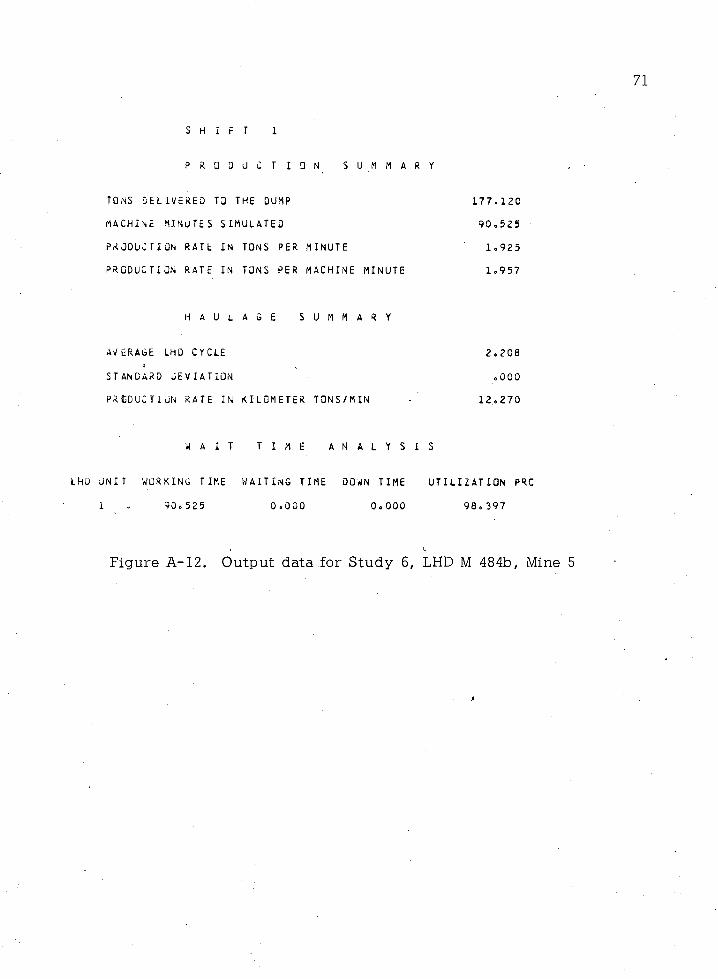
71
S H I F T 1
P R O D U C T I Q N ] S U M M A R Y
TONS DELIVERED T3 THE DUMP 1 7 7 . 1 2 0
MACHINE MINUTES SIMULATED 9 0 . 5 2 5
PRODUCTION RATE IN TONS PER MINUTE 1 . 9 2 5
PRODUCTION RATE IN TONS PER MACHINE MINUTE 1 . 9 5 7
H A U L A G E S U M M A R Y
AVERAGE LHD CYCLE 2 . 2 0 8i
STANDARD DEVIATION . 0 0 0
PR CDUC TI UN RATE IN KILOMETER TONS/MIN - 1 2 . 2 7 0
W A I T T I M E A N A L Y S I S
LHD UNIT WORKING TIME WAITING TIME DOWN TIME UT IL IZATION PRC
1 . 9 0 . 5 2 5 0 . 0 0 0 0 . 0 0 0 9 8 . 3 9 7
L
Figure A -12. Output data for Study 6, LHD M 484b, Mine 5

APPENDIX B
INPUT AND OUTPUT DATA FOR
SENSITIVITY ANALYSIS STUDY
72
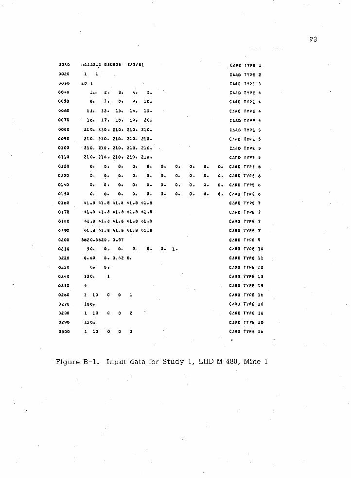
0010 nAZ&815 GEORGE 2/3/81 CARD TYPE 10020 1 1 CARO TYPE 20030 20 1 CARO TYPE 30040 lo. 2. 3. 4. 5. CARO TYPE 40050 6o 7 o 8. 9 o 10. CARO TYPE 40060 1 lo 12. 13. 14. 15. CARO TYPE 40070 16. 17. 18. 19. 20. CARD TYPE 40060 210. 210. 210. 210. 210. CARD TYPE 50090 210. 210. 210. 210. 210. CARO TYPE 50100 210. 210 . 210. 210. 210. CARO TYPE 50110 210. 210. 210. 210. 210. CARD TYPE 50120 0o 0. 0. 0. 0. 0. 0. 0. 0. 0. CARO TYPE 60130 0. o. 0. . 0. 0. 0. 0. 0. 0. 0. CARO TYPE 60140 0. 0. 0. 0. 0. 0. 0. 0. 0. 0. CARD TYPE 60150 0. 0. 0. 0. 0. 0. 0. 0. . 6. 0. CARO TYPE 60160 41.8 41. 8 41.8 41.8 41.8 CARO TYPE 70170 41.9 41.8 41.8 41.8 41.8 CARO TYPE 70180 41.8 41.8 41.8 41.8 41.8 CARD TYPE 70190 41 .8 41.8 41.8 41.8 41.8 CARO TYPE 70200 3620. 3620 . 0.97 CARD TYPE 90210 so. 0. 0. 0. 0. 0. 1. CARD TYPE 100220 0. 69 0. 0.42 0. CARO TYPE 110230 4. 0. CARO TYPE 120240 330. 1 CARO TYPE 130250 4 CARO TYPE 150260 1 10 0 0 1 CARO TYPE 160270 100. CARD TYPE 100280 o © 0 2 - CARO TYPE 160290 150. CARO TYPE 100300 1 10 0 0 3 CARO TYPE 16
Figure B -l. Input data for Study 1, LHD M 480, Mine 1
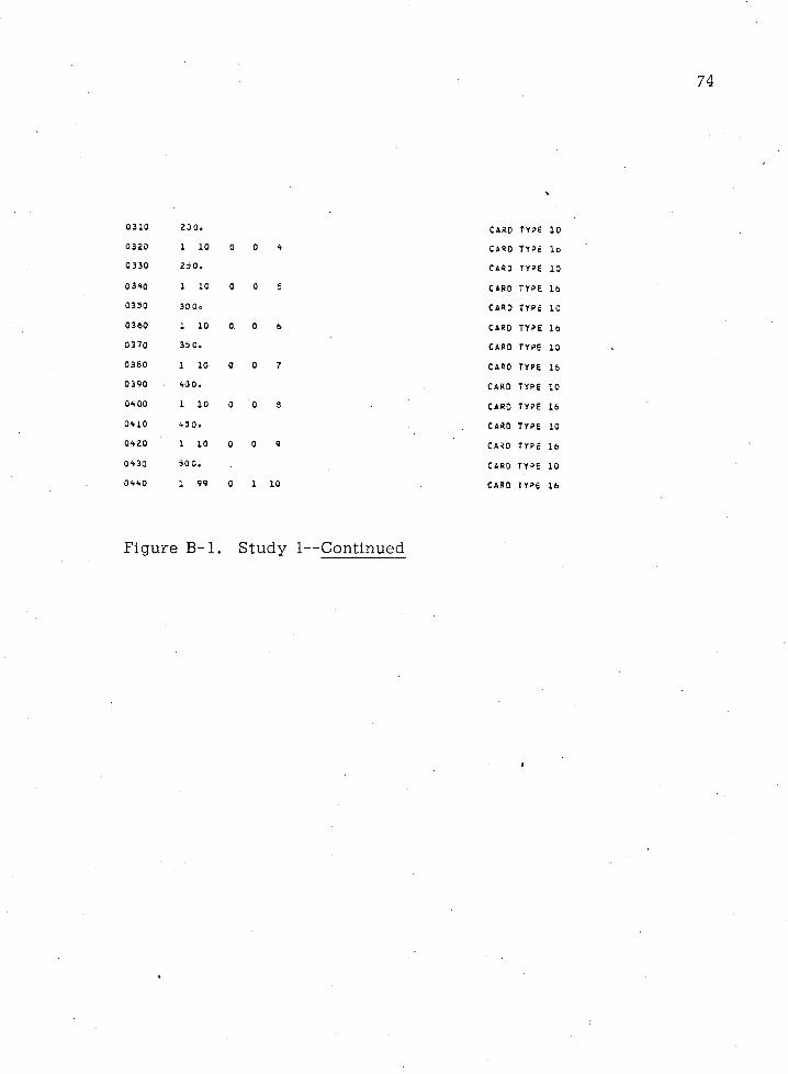
74
0310 200. CARD TYPE 100320 1 10 0 0 4 CARO TYPc lb0330 250. CARO TYPE 100340 1 10 0 0 5 CARD TYPE 160350 300. CARD TYPE 100360 1 10 0 0 6 CARD TYPE 160370 35 0. CARD TYPE 100380 1 10 0 0 7 CARD TYPE 160390 400. CARD TYPE 100400 1 10 0 0 8 CARD TYPE 160410 450. CARD TYPE 100420 1 10 0 0 9 CARD TYPE 160430 500. CARD TYPE 100440 1 99 0 1 10 CARD TYPE 16
Figure B -l. Study 1—Continued

0010 M A Z A B I S G E O a G E 2/3/91 CARO TYPE 10020 1 1 CARD TY9E 20030 20 1 C A R O TY9E 30040 lo 2. 3. 4. 5. CARD TYPE 40050 6o 7 . 8, 9. 10. C A R O TYPE 40060 l i e 12. 13. 14. 15. C A R D TYPE 40070 16, 17. 16. 19. 20. CARD TYPE 40080 25 0, 280 . 280, 290. 260. C A R D TYPE 50090 2d 0o 280. 260. 280. 250. C A R O TYPE 50100 280, 280 , 280. 290. 280. CARD TYPE 50110 290, 260 . 280, 280, 280, C A R O TYPE 5
0120 0, 0 . 0 . , 0 , 0 . 0 . 0 . 0 . 0 . 0 . CARD TYPE 6
0130 Go 0 . 0. 0 . 0. 0 . 0 . 0 . 0 . 0 . CARD TYPE 60140 0 , 0 . 0. 0 . 0 , 0. 0. 0. 0. 0 . CARO TYPE 60150 6, 0. 0 . 0 . 0 , 3. 0 . 0 . o . 0. CARD TYPE 60160 25 .2 25.2 25.2 25.2 25.2 CARO TYPE 70170 25,2 25.2 25,2 25,2 25,2 CARD TYPE 70180 25 ,2 25.2 25.2 25,2 25.2 CARD TYPE 70190 25 ,2 25. 2 25.2 25.2 25.2 CARO TYPE 70200 3620,3620, .97 CARD TYPE 90210 5 0, 0 . 0 . 0o Qo 0 * 1 0 CARD TYPE 100220 0, 60 0 . 0.42 0 . CARO TYPE 110230 3,15 0 , CARD TYPE 120240 330, 1 CARO TYPE 130250 4 CARD TYPE 150260 1 10 0 0 1 CARO TYPE 160270 100. CARO TYPE 100280 1 101 0 0 2 CARO TYPE 160290 150, CARD TYPE 100300 1 10 0 0 3 CARO TYPE 16
Figure B-2. Input data for Study 2, LED M 484a, Mine 2

76
0310 200. CARD TYRE 100320 1 10 0 0 4 CARO TYPE 160 330 250. CARD TYPE 100340 1 10 0 0 5 CARD TYPE 160350 300. CARD TYPE 100360 1 10 o' 0 6 CARD TYPE 160370 350. CARD. TYPE 100380 1 10 0 0 7 CARD TYPE 160390 400. CARD TYPE 100400 1 10 0 0 8 CARD TYPE 160410 450. CARD TYPE 100420 1 10 0 0 9 CARD TYPE 1604 30 500. CARD T Y°E 100440 1 99 0 1 10 CARD TYPE 16
Figure B-2. Study 2—Continued
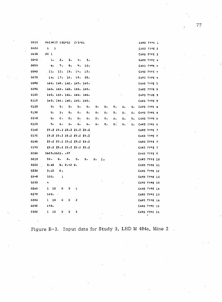
0010 fUZARIS GEORGE 2/3/81 CARO TY3E 10020 1 1 CARO TYPE 20030 20 1 CARO TYPE 30040 lo 2, 3. 4. 5. CARO TYPE 40050 6o 7, 8, 9, 10. CARO TY°E 40060 lie 12. 13, 14. 15. CARO TYPE 40070 16o 17, 18 . 19. 20. CARO TYPE 40080 16 Oo 160 , 160, 160 o 160. CARO TYPE 50090 16 0o 160, 160, 160. 160 o CARD TYPE 50100 160, 160 , 160, 160. 160. CARO TYPE 50110 16 0e 160 , 160 o. 160. 160. CARD TYPE 50120 Oo 0o 0, 0, 0, 0. 0. Oo 0. Oo CARO TYPE 60130 Oo 0. 0o 0, 0. 0. 0. 0. 0. 0. CARO TYPE 60140 Oo 0. 0o Oo Oo Oo Oo Oo Oo 0. CARO TYPE 60150 Oo 0. 0, 0. 0, 0. 0. 0. 0. ' Oo CARD TYPE 60160 25o2 25,2 25,2 25.2 25.2 CARO TYPE 70170 25 o2 25.2 25.2 25.2 25.2 CARD TYPE 70180 25 o2 25 6 2 25,2 25,2 25.2 CARO TYPE 70190 25,2 25,2 25.2 25.2 25.2 CARO TY»E 702 00 3620,3620. .97 CARD TYPE 90210 50 » 0. Oo 0. Oo Oo lo CARO TYPE 100220 Oo 60 0. 0 • 42 Oo CARD TYPE 110230 3.15 0 o CARD TYPE 120240 33 Oo 1 CARD TYPE 130250 4 CARO TYPE 150260 1 10 0 0 1 CARO TYPE 160270 100, CARO TYPE 100280 1 10 0 0 2 CARD TYPE 160290 15 Oo CARO TYPE 100300 1 10 0 0 3 CARO TYPE 16
Figure B-3. Input data for Study 3, LHD M 484a, Mine 2

78
0310 200. CARO TYPE0320 1 10 0 0 4 CARD TYPE0330 250. CARD TYPE0340 1 10 0 0 5 CARD TYPE0350 300. CARD TYPE0360 1 10 0 0 6 CARD TYPE0370 35 0. CARO TYPE0380 1 10 0 0 7 CARD TYPE0390 40 0. CARD TYPE0400 1 10 0 0 8 CARD TYPE0410 450. CARO TYPE0420 1 10 0 0 9 CARD TYPE0430 500. CARO TYPE0440 1 99 0 1 10 CARO TYPE
Figure B-3. Study 3—Continued
10
1610
1610
1610
1610
16101610
16

0010 HAZ Aft IS GEuRGc 2/3/81 CARD TY»E 10020 1 1 CARD TYPE 20030 20 1 CARO TYPE 30040 lo 2. 3. 4. 5. CARD TYPE 40050 6o 7. 8. 9. 10. CARO TYPE 40060 lie 12. 13. 14. 15. CARD TYPE 40070 16. 17. 18. 19. 20. c a r d TYPE 40060 230. 260 . 260. 280. 230. CARO TYPE 50090 230. 280. 290. 280. 230. CARD TYPE 50100 290. 280 . 290. 280. 280. CARD TYPE 50110 230. 280 • 280. 280. 280. CARO TYPE 50120 0. 0. 0. 0. 0. 0. 0. 0. 0. 0. CARO TYPE 60130 0. 0. 0. 0. Go 0. 0. 0. 0. 0. CARO TYPE 60140 0. 0 . 0. 0. 0. 0. 0. 0. 0. 0. CARO TYPE 60150 0. 0 . 0. 0, 0. 0. 0. 0. 0. „ ' 0. CARO TY»E 60160 29 ,2 29.2 29.2 29.2 29.2 CARD TYPE 70170 29.2 29.2 29;2 29,2 29,2 CARO TYPE 70180 29.2 29.2 29.2 29.2 29.2 CARO TYPE 70190 29 .2 29.2 29.2 29.2 29.2 CARD TYPE 70200 3620.3o20 o lo CARO TY*E 90210 50. 0. 0. 0. 0. 0. 1. CARO TYPE 100220 0. 37 0. 0.34 0, CARO TYPE 110230 2.65 0. CARO TYPE 120240 330. 1 CARO TYPE 130250 4 CARD TYPE 150260 1 10 0 0 1 CARD TYPE 160270 100. CARO TYPE 100260 1 10 0 0 2 CARO TYPE 160290 15 0. CARO TYPE 100300 1 10 0 0 3 CARO TYPE 16
Figure B-4. Input data for Study 4, LHD M 74a, Mine 3

80
0310 200. CAAO TYPE0320 1 10 0 0 4 CARD TYPE0330 250. CARD TYPE0340 1 10 0 0 5 CARD TYPE0350 300. CARD typ e
0360 1 10 0 0 6 CARD TYPE0370 35 0. CARD TY»E03 80 1 10 0 0 7 CARD TYPE0390 400. CARD TYPE0400 1 10 0 0 8 CARD TYPE0410 450. CARD TY = E0420 1 10 0 0 9 CARO TYPE04 30 500. CARD TYPE0440 1 99 0 1 10 CARD TYPE
10
1610
1610
1610
161016
10
1610
16
Figure B-4. Study 4—Continued

0010 RAZ ARIS GcORGE 2/3/81 CARO TYPE 100 20 1 1 CARD T Y 9E 2
0030 20 1 CARO TYPE 30040 1. 2 . 3. 4 o 5. CARD TYPE 40050 Oo 7 o 8 . 9 o 1 0 . CARD TYPE 40060 1 1 0 12 o 13. 14. 15 o CARD TYPE 4
0070 16. 17. 18. 19. 2 0 . CARD TYPE 40080 1 2 0 . 1 2 0 , 1 2 0 . 1 2 0 . 1 2 0 . CARD TYPE 50090 12 0 o 1 2 0 , 120 o 1 2 0 . 1 2 0 . CARD TYPE 50 1 0 0 1 2 0 . 1 2 0 . 1 2 0 . 1 2 0 . 1 2 0 . CARD TYPE 50110 12 0 . 1 2 0 . 1 2 0 . 1 2 0 . 1 2 0 . CARD TYPE 50120 Oo Oo 0 . Oo Oo Oo Oo Oo Oo 0 . CARD TYPE 6
0130 Oo Oo Oo 0. Oo 0. Oo Oo 0. Oo CARD TYPE 6
0140 Oo 0. Oo 0. 0, 0. 0. Oo 0. 0. CARO TYPE 60150 Oo 0 6 Oo Oo 0, Oo Oo Oo o'. - ■ Oo CARD TY'E 60160 45 08 45.8 45,8 45.8 45.3 CARD TYPE 70170 45 .8 45. 8 45.8 45.8 45.8 CARO TYPE 70180 45 .8 45. ti 45 0 8 45 e 8 45,8 CARD TYPE 70190 45 .8 45. 8 45.8 45 . d 45.8 CARD TYPE 7
0200 362 0.3620 .<,972 CARD TYPE 90210 5 Oo 0 0 0. 0 0 • 0. Oo 1 0 CARO TYPE 100220 Oo 62 0. 0.42 0. CARD TYPE 110230 5.72 0 0 CARD TYPE 120240 33 Oo 1 CARD TYPE 130250 4 CARO TYPE 150260 1 10 0 0 1 CARO TYPE 160270 100. CARD TYPE 100280 1 10 0 0 2 CARD TYPE 160290 150. CARO TYPE 100300 1 10 0 0 3 CARD TYPE 16
Figure B-5. Input data for Study 5, LHD M 74b, Mine 4

82
0310 230. CARD TYPE0320 1 10 0 0 4 CARO TYPE0330 250. CARO TYPE0340 1 10 0 0 5 CARD TYPE0350 300. CARD TYPE0360 1 10 0 0 6 CARD TYPE0370 350. CARD TYPE0360 • 1 io 0 0 7 CARD TYPE0390 400. CARD TY°E0400 1 10 0 0 3 CARD TYPE0410 450. CARD TYPE0420 1 10 0 0 9 CARD TYPE0430 500. CARD TYPE0440 1 99 0 A 10 CARD TYPE
Figure B-5. Study 5—Continued
10
1610
1610
1610
1610
1610
1610
16
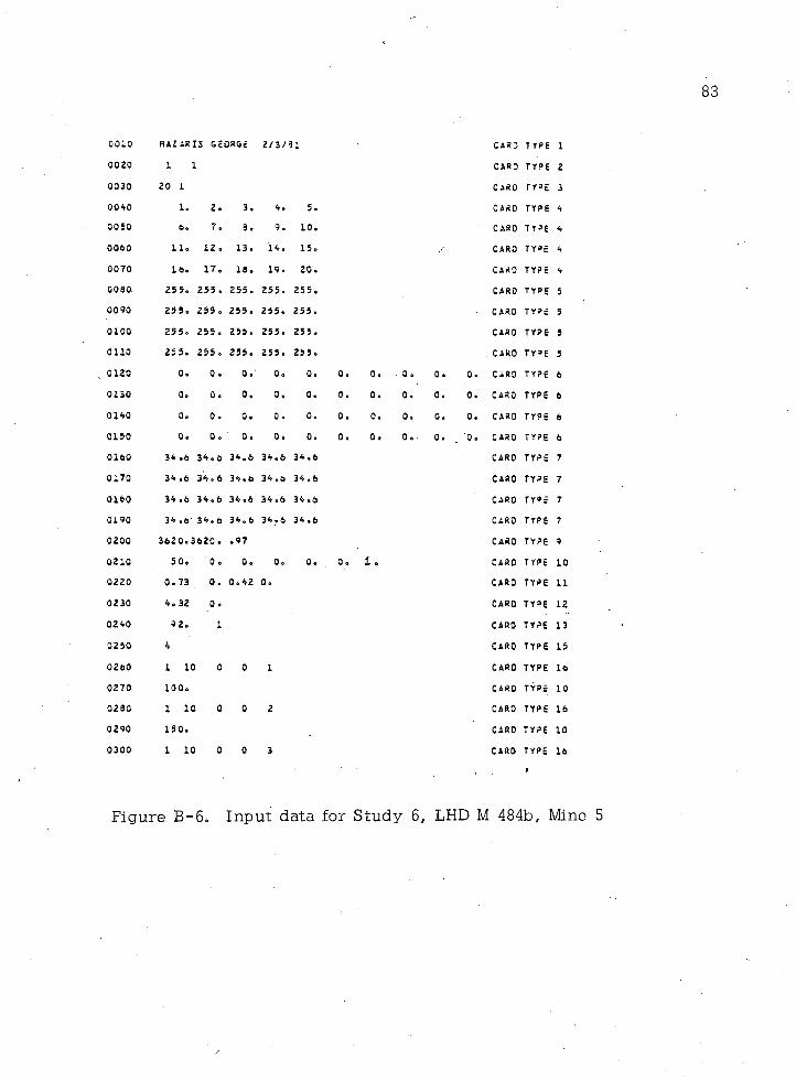
83
C010 MAZARI 5 GcORGe 2/3/51 CARO TYPE 100 20 1 1 CARO TYPE 20030 20 1 CARO TYPE 30040 1. 2. 3. 4. 5. CARD TYPE 40050 tie 7. 3. 9. 10. CARD t y p e 40060 H o 12. 13. 14. 15. CARO TY»E 40070 16. 17. 18. 19. 20. CARO TYPE 40080. 255. 255 . 255. 255. 255. CARD TYPE 50090 25 5 o 255 . 255. 255. 255. CARD TYPE 50100 255. 255 . 255. 255. 255. CARD TYPE 50110 255. 255 . 255. 255. 255. CARO TYPE 50120 0. 0 . 0.' 0 , 0, 0. 0. 0 . 0. 0. CARD TYPE 60130 0. 0 . 0 . 0 . 0 . 0 . 0 . 0 . 0. 0 . CARD TYPE 60140 0. 0 . 0 . 0. 0 . 0 . 0 . 0 . 0 . 0 . CARD TYPE 60150 0 . 0 . ' 0. b. 0. 0 , 0. 0 . 0. 0 . CARO TYPE 60160 34 .6 34.6 34.6 34,6 34.6 CARD TYPE 70170 34 .6 34 o 6 34.6 34.6 34.6 CARO TYPE 70160 34 .6 34.6 34,6 34.6 34 .6 CARD TYPE 70190 34 .6 34.6 34.6 34.6 34.6 CARO TYPE 70200 3620.3620. .97 CARD TYPE 90210 5 0, 0 • 0. 0. . o, . 0 . I. CARO TYPE 100220 0.73 0. 0.42 0 . CARD TYPE 110230 4.32 0. CARO TYPE 120240 92. 1 CARO TYPE 130250 4 CARD TYPE 150260 1 10 0 0 1 CARO TYPE 160270 100. CARO TYPE 100280 1 10 0 0 2 CARD TYPE 160290 150. CARD TYPE 100300 1 10 0 0 3 CARD TYPE 16
Figure B-6. Input data for Study 6, LHD M 484b, Mine 5

84
0310 200. CARD TYPE 100320 1 10 0 0 4 CARD TYPE 160330 250, CARD TYPE 100340 1 10 0 0 5 CARD TYPE 160350 300. CARD TYPE 100360 1 10 0 0 6 CARD TYPE 160370 350. CARD TYPE 100 360 1 10 0 0 7 CARD TYPE 160390 400. CARO TYPE 1004C0 1 10 0 0 8 CARD TYPE 160410 450. CARD t y p e 100420 1 10 0 0 9 CARO TYPE 160430 500. CARO TYPE 100440 1 99 0 1 10 CARD TYPE 16
Figure B-6. Study 6—Continued

85
AVERAGE LHD SPEED
o •*
500 o CO
o • *
# o o # 0* o e # * # g & * # e * e # c * # e c e o 0 4 50 O 00 * 4%0 00#C*00
0 5? #0*9*0 ##*##* # # # $ # # # 0 0 # # *
*o00#*00**0000000 OoOO00000000
400oG0 0 000 0 9000o o o o o o o o # 0 0 o o o o o o o OOO0 0 0 0 *0 9 0 0 0 0 # o o o o o o o o o o o o o 00 0 # 0900 0 0 * 0 0 * 0 0 OOO # 000 0 o
3 50 o 00 * 0 0 o o o o # o o o o o o o o o o o o o o o #9 9009 0 099 009990999 000 00 9 0 9OOO900 0 0 9 0 0 9 0 0 0 9 0 0 00 000
300o00 0 0 0 0 0 0 0 0 9 0 9 0 0 0 0 0 0 9 0 0 0 9 90 0 0 0 0 9000 000009 o o o o o o o o900 9 0 9 * 9 9 9 9999 90099999 09
£ 50 O 00 OOO 90# 0#9 009000 00# 00000 0 0 OOOOOO 0009 0 0 O OOoooo90
OOO0 0 0 9 0 9 0 0 9 0 0 9 OOOO
200 O 00 00 0 00 0900 000900 o o o o009909 90 0009 909009 9o0009 0 0 0 * 0 0 o o o o o o 0
150 o 00 999 900900 909990 90 00 OOOOOo OOOOOO 0 0 0999990 00 0 09 9
100 o 00 0 * 9 0 9 0 0 0 9 0 0 0 090900900*0**0 9 0 OOOO
50o 00 o o o o o o *o 0 O 90 9 0009 OOOOOO 4*00000 OOOOOOOO OOO 009 <»0 OOOOOOOO '
Oo 2 5 0 . 5 0 0 . 7 5 0 . 1 0 0 0 .
TONS DELIVERED IN THE DUMP
Figure B-7. Histogram for average speed-production per shiftsensitivity analysis, Study 1, LHD M' 480," Mine 1

8 6
A V E i U
5 0 0 o 0 0
4 5 0 o 0 0
4 0 0 oOO
3 5 0 o 0 0
3 0 0 0 0 0
250 o 00
200000
1 5 0 , 0 0
1 0 0 , 0 0
5 0 , 0 0
iE LHO SPEED
t?*00* OOOOOO0 * 4 * 0 * 0 * 0 * 0 4 * 0 0 0 0 * * 0 0
o
0*** 000000 000 000 *00*0 * 0* 0* 0*00 000**0 * 0 0 0 0 «? 00 0*0i?** 00000o 00000 0 0* 0 * 0 0 0 0 0 0 0 0 * 0 0 * * 0 0 00 0 * 0 0 * 0 * 0 0 0 * * 0 0 OOO*0 * 4 0 0 * * 0 0 0 * * 0 0 0 0*0.*
o
00 0 0 000* 00* 00000*00 Op* *000000000*0 0 0 0 00* 000000 000000 000 o
00 0 * * 0 0 0 0 0 0 0 0 0 0 0 0 00000000000* 000oOOO 0000*0000000 oo
o
0 0 * 0 0 0 0 0 0 OOO00 00* 0 0 0 0 0 0 0 0 0 0 0 OOO0 * 0 0 0 0 o o o o *000 0 0 0 0 0 0 0 0 0 0 0P O O * 0 0 0 0 0 0 0 0 000 0 0 0 0 0 0 OOO
o
00 0 * 0 0 0 0 0 0 *
0 0 * 0 0 0 0 0 0 0
0 0 * OOOOOO o
o
o
00*00000 0 0 0 0 * 0000*0*0 Ioo
0 0 * 0 0000000 0 0 0 0OOP 0 0 0 * 0 0 4 * 0 0 0 0 0 0 0 0 4 0 0 0 0 0 * 0 0 * 4 * 0 0 0 00 00 0* 4
Oo. 2 50 o 500o 750 0 lOOOo
TONS DELIVERED IN THE DUMP
Figure B-8. Histogram for average speed-production per shiftsensitivity analysis. Study 2, LHD M 484a, Mine 2

87
AVERAGE LHD SPEED
oo
5 0 0 o 00 *oo000**0 oooooo ooooooooo00OoOooooooooooooooooooooo
450 O 00 000 oooooo oooooooooooooooO O0 OOO OOO OOOOOO 0 0 0 * 0 * 0 * 0o00 0 0 0 0 * 0 0 0 o o o o o o o o o o o o o o o
4 0 0 o 0 0 * 0 0 0 0 * 0 0 0 OOOoOO 0 0 0 0 0 . 0 0 0 0 * * o OOOOOO 0 0 * 0 0 0 o o o o o o o o o 0 0 .
0 0 0 OOOOOO 0 0 0 * 0 0 * 0 0 OOOOOO350 0 00 0 00ooooooooooooooooooooo
C$ 0 0 OOOOOp o o o o o o OOOOOOOOO 00 - 0 0 0 OOOOOO * 0 0 * 0 0 o o o o o o o
3 0 0 o 0 0 o o o o o o o o o o o o o o o o o o o o o *0*0 oooooo 000*00 ooooooo 0 0O O O * 0 0 0 * 0 0 0 * 0 0 0 o o o o o o
250 O 00 ooooooooooooooooooooo ********************* o o* * * * * * * * * * * * * * * * * * *
200 o 00 ooooooooooooooooooo * * * * * * * * * * * * * * * * * * *0o* * * * * * * * * * * * * * *
150o00 ooo oooo**************p**oooooo 0 0* * * * * * 0 * * 0 0 0
100 oOO oOoooooostoo** * * * * * * * * * * *0 ' o0 * 0 0 0 0 0
50 o 00 ooooooo ooooooo000 0*00*0 <*00000 ooo0«>00 0*00*0*<• 0000*0ooo<•Oo 2 5 0 o 5 0 0 o . 7 5 0 o lOOOo
TONS DELIVERED IN THE DUMP
Figure B-9. Histogram for average speed-production per shiftsensitivity analysis, Study 3, LHD M 484a, Mine 2
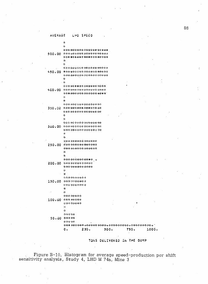
8 8
average LHO SPEED
*o
500 o 00 ooao**oeoo*oocco#9**o0o # o * # # * p o $ o # # # e * o * & o
A50 o 00 $ o o * o o o * o o c * # c * $ o o o *e e o # o o e * o & # e a o # & # o c OOo0 # e c * $ $ * 0 0 $ # e § 0 0 0 # #
4 0 0 oOO o o o c e o o o p e a e c e o o o * *
o0o c o o o o e c c o o e o e o o *
350 o 00 o o o & o o e o e o e # # # * * # o * o o o o o o o 0 * * 0 0 * oo o o* 0 * * 0 0 0 0 0 * 0 0 * 0 0 0 #
300 o 00 *o o o o o o o o o o o o o o o oOOO0 0 0 * 0 0 0 0 0 * * 0 0 0oo00 0 0* 0 * 0 0 * * * 0*0
250 o 00 ooo oooooo ooooooOOO***********0o00 0 0 * 0 0 0 0 0 0 0 0 0 e>
2 0 0 o 00 0 0 0 0 * 0 * * 000*00 0 * o o o o o o * * * *o0o o o o * * o * o 0
150 o 00 * * # o o o o o o ** * * * * * * * * *
*oo o o * * * * *
I C O o 00 o o o o o o * *O O O * # # * * <*00 0 * 0 0
50o 00 ****** * * * *
0*0 ooo*#* 4,#*#** *00*4,ooo*o#o#*<,ooo*ooo** «> •Oo 250. 500. 750, 1000.
TONS DELIVERED IN THE DUMP
Figure B-10. Histogram for average speed-production per shiftsensitivity analysis. Study 4, LHD M 74a, Mine 3

89
AVEkAGE LHO SPEED
*5 00 o 00 * # * # ? * * $ * # # *
o <19 o e e o e * 9999 # * 9 9 9 9 9 9 9 9 9 9 9 9 9 9 9 9 9 9 0 9 3 0 9 9 9 9 * 9 9
09 9 9 9 0 9 * * * 0 0 * * 9 * * * * 9 * * 9 * * 9 9 9 * * * * * 0 9 0 * * 9 * 0 * * *
450 * 00 c 9 * * c * c o o * c o * * o o o e o e O e o o o c O c e c c o e o o o o c c e c o *9 00 *09 0 * 0 9 0 * 0 00 9 0 0 0 0 * * * * * * * * * * * * * * * * * * * * * 0 *
o
*0 9 0 9 0 * 0 0 0 9OO*?i?0 9O0OPOOOCiO90^0 00 9 00*<70 0* 9 * 0 *
4 0 0 o 00 ^ 0 0 9 * * 9 0 * 0 0 * 0 * 0 9 0 0 0 * 0 0 * 0 0 0 * 0 0 0 0 * 0 0 * 0 0 * * 0 * 0 *0 0* * 9 9 0 * 9 0 0 0 0 99 9 9 * 0 * 9 * * * * * Oo** 9 0 o * * * OOOOOO0
o
o
000 * 0*000 * * * * * * * 0 * * 0 0 0 * 0 0 0 * 0 * 0 0 * 0 * 0 0 0 0 * 0*0 03 5 0 0 00 0*000*000OOOOOOOOO000000*000000000000000000
0 0 0 0 0 0 * * 9 0 0 0 0 0 * 0* 0 0 0 * 0 * 0 0 0 0 * * 0 * 0 0 0 * * 0 * 0 0 0 0 *
O
0
0 9 * 0 0 * 0 0 0 0 0 0 * 0 * 0 0 0 0 0 0 0 9 * 0 0 0 0 0 0 0 * * 0 0 0 * 0 * 0 0 * 0 300 o 00 0 0 0 0 0 0 * * 0 0 0 0 0 0 0 0 0 0 0 * 0 * * 0 0 0 0 0 * 0 0 0 0 0 0 0 0 0 0 0 0 0 *
9 9 9 090 99 9 0 9 9 9 9 9 9 9 0 9 9 0 9 0 0 0 0 * 0 * 9 0 * 9 0 * 0 0 * 0 0 99 0
0
0 .
0 0 0 0 0 * 0 0 0 0 * 0 0 0 0 0 * * 0 0 0 0 0 0 0 * 0 0 0 0 0 * 0 0 * 0 0 0 0 * *
2 50 o 00 * 0 0 0 * * 9 0 0 * 9 9 9 9 * 9 * 9 9 0 0 * * 0 0 9 9 0 0 * 0 * 9 0 9 0 * 0 0 90*** ****** *00*** *********0 0**0o***********0
*0*0 0*0*0900 9*9* 0*09*999 9 9 9909*9 990*9 *0*
200 0 00 * 0 * 0 * * * 0 * 0 * 9 * 0 9 0 * 0 0 9 0 0 * * 0 0 * 0 * 0 * * 9 0 * * * * *
0 0* * 0 0 * * 0 * 0 0 * * 0 0 * 0 0 0 9 0 0 0 * 0 0 0 * * 0 * * 0 * * * * *
o
o0 0 * 0 0 0 * 0 0 0 0 0 * 0 0 o * * * * * * 0 0 * * * * * * 0 *0
150 0 00 * * * *0 * * 0 * 9 0 0 * 0 * * * 0 0 0 0 0 * * 0 0 * 9 * * 0 * *0 0 0 0 * 9 * 9 0 * * 9 0 * 0 * * * * * 0 * 0 * * 0 0 * 0 0 0 * 0
0
0000 ****** 0*000000**00*00
100 6 00 0 * 0 * 0 * * 0 0 * 0 0 * 0 * O O O * * * * * **09*0 0 9*0909*000*9*00 099 *00 * 0 * 0 * * 0 0 0 0 9 * 0 *
50 O GO 9 909*9*09 *999*9 0 0 0 .0* 0 * 0 * * 0***00 * 0 0 * 0 * 0 0 <>0*9*0 9 0 0 0 * 0 0 0 9 0 * 0 0 0 * 9 * 0 0 0 * 0 0 0 * 0 * 0 0 * 0 0 0 0 *
Do 2 5 0 . 5 0 0 . 7 5 0 . 1 0 0 0 . 1 2 5 0 .
TONS DELIVERED IN THE DUMP
Figure B - l l . Histogram for average speed-production per shiftsensitivity analysis. Study 5, LHD M 74b, Mine 4

90
a v e r a g e lho s p e e dO$
5 0 0 oOO ».** * * » $ * *
oo
4 5 0 o 0 0 * 0 9 * * 9 * * #
*
O* 9 * p O * 9 *
4 0 0 o 0 0 * * * * * * * ** 9 9 9 * 9 9 9 **** * * * * * * *
3 5 0 O 00 9 9 9 * * 9 0 0 * * * * * * * *** _
* * * * * * *
3 0 0 0 0 0 * * * * * * ** * * * * * *0
o* * * * * *
2 5 0 0 0 0 * * * * * ** * * * * **0* * * * * *
2 0 0 o 0 0 0 0 * 0 * ** * * * * *
***** **
1 5 0 0 0 0 09* * * * *00* 9 9 *
1 0 0 o 0 0 0 * * 09 * 9 *0 '9***
50 o 00 000 * * *9 9 9 9 * * * 9 * * * 9 * 9 9 * * * * 4 9 9 9 9 9 9 9 * 9 4 9 9 0 * * * * * * 40 . 2 5 0 . 5 0 0 . 7 5 0 . 1 0 0 0 .
TONS DELIVERED IN THE DUMP
Figure B-12. Histogram for average speed-production per shiftsensitivity analysis, Study 6, LHD M 848b, Mine 5

APPENDIX C
USER'S MANUAL FOR PROGRAM MINPIL
91

92
TABLE OF CONTENTS
Section Page
1. PROGRAM IDENTIFICATIONS . 94
1.1 Program T i t l e . 941.2 program Code Name ..................... 941.3 Program C oordinator..................................................... 941.4 Program Writer ............................................................. 941.5 Program Documentation................................................. 941.6 Organization .......................................................... 941.7 Date ......................................... 941.8 Updates, Versions . . . .................................... 941.9 Source Language ............................. 941.10 Availability................................. 941.11 A b stract..................................... 94
2. ENGINEERING DOCUMENTATION..................................................... 95
2.1 Narrative Description...................................................... 952.2 Method of Solution ......................... 96
2.2.1 Input Variables ................ 962.2 .2 Program MINPIL O u tp u t..............................1022.2 .3 Algorithm Formulation ..................... 1032.2 .4 Simulation P h ilo so p h y . 1092.2 .5 Program Constants ......................109
2.3 Program C ap ab ilities............................................ . . I l l2.3 .1 Deterministic Sim ulation . I l l2.3 .2 Range of Variables. . . . . . . . . . I l l2 .3 .3 Limitations and Restrictions of
Methods of A n alysis..................................I l l2.3 .4 Program S e n s it iv ity ......................................1122.3 .5 Handling Varied Operating
C haracteristics.................... . . . . ’ 1142.4 Data Inputs ..................................... 117
2.4.1 Introduction....................... 1172.4 .2 Data Input Description by
Card Type . . . . . . . . . . . . 1182.5 Program Options ..................... 121
2.5.1 Multiple Runs . ......................................... 1212.5 .2 Conventional and Continuous
Methods ......................................1252.6 Printed Output ..................................... 1252.7 Other O u tp u ts .................................................................. 1272.8 Flow Chart . . ..................................... 1302.9 Sample Runs ................................. 130
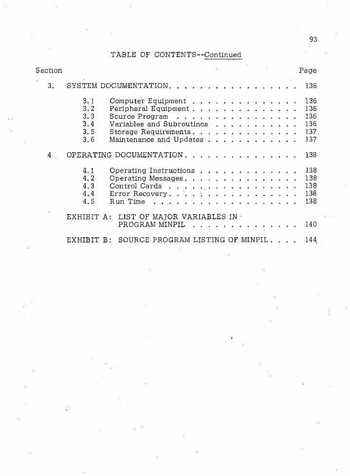
93
TABLE OF CONTENTS—Continued
Section " Page
3. SYSTEM DOCUMENTATION. .......................................................... 136
3.1 Computer E quipm ent..................................... 1363.2 Peripheral Equipment..................................... 1363.3 Source Program . . . ................................. 1363.4 Variables and S u b r o u tin e s ............................. 1363. 5 Storage Requirements. . . ...................................1373.6 Maintenance and U p d a tes.............................................. 137
4 OPERATING DOCUMENTATION ................................. 138
4.1 Operating In stru c tio n s .................................................. 1384.2 Operating M essages. ...............................1384.3 Control Cards ......................... 1384.4 Error Recovery. ............................................... 1384.5 Run Time . .................................................................. 138
EXHIBIT A: LIST OF MAJOR VARIABLES IN •PROGRAM M IN PIL........................ 140
EXHIBIT B: SOURCE PROGRAM LISTING OF MINPIL . . . . 144

94
SECTION 1
PROGRAM IDENTIFICATION
1.1 Program T itle: LHD Simulator
1.2 Program Code Name: MINPIL
1.3 Program Coordinator: Young C. Kim
1.4 Program Writer: George M. Mazaris
1.5 Program Documentation: George M. Mazaris
1.6 Organization: Department of Mining and Geological Engineering,The University of Arizona,Tucson, Arizona 85721
1.7 Date: October 30, 1980
1.8 Updates, V ersions: No updates, Version 0
1.9 Source Languages: FORTRAN IVCDC 6400 Computing System
1.10 Availability: Limited
1.11 Abstract:
This program simulates the loading and secondary haulage operation of an underground mine which utilizes load-haul-dump (LHD) units in loading and secondary haulage, given the LHD characteristics and the mine lay-out elements.

95
SECTION 2
ENGINEERING DOCUMENTATIONS
2.1 Narrative Description
The introduction of high mechanization in underground mines has replaced conventional methods in development and stoping operations. Trackless mining equipment, because of its unique characteristics, has contributed to the mechanization of loading, dumping, and hauling operation.
Load-haul-dump (LHD) units with their high productivity and flexibility and low maintenance costs are operating, as loading and secondary haulage units in various room-and-pillar mechanized cut and fill, sublevel caving, sublevel stoping, block caving, and development work.
Program MINPIL attempts to simulate the loading and secondary haulage operations of an underground mine where LHD equipment is in use. The program is able to handle conventional or continuous room-and- pillar methods, pull-push or circular LHD trips, development work, and removal of a material pile to a new position or draw point.
Because LHD delays are an important factor in the application of LHD units, delays are taken into account by using mechanical availability as a variable in the program. Queueing time due to a no-passing policy and the operation of the miner are also considered.
Required input data include probability distributions for the basic LHD-related variables (payload, speed, loading and dumping times, e tc .) and deterministic values for the other LHD-related variables (acceleration, deceleration, e tc .) and for the non-L HD-related variables (mine lay-out characteristics, cut sequence, e tc .) . Output is a sh ift-by-shift report which is composed of a productivity analysis, a haulage summary, and a

96
time analysis for each LHD unit. At the end of the simulation, a general simulation report is provided.
The user has the option of performing multiple runs and sensitivity analysis to evaluate the effect of some variable on shift production. The program generates histograms to illustrate the results of the multiple runs.
2. 2 Method of Solution
The method of solution is composed of definitions of input variables and output data, the development of the program algorithms, and clarification of the program simulation language.
2. 2.1 Input Variables
Mechanical Availability. The mechanical availability of an LHD unit or miner is defined as the percentage of time the unit is moving and not waiting or down. The availability value for a particular unit is obtained by using data from the maintenance department.
Loading Time. The loading time is the time it takes to load an LHD unit. The value for this variable is calculated from time studies and is composed of two parts: (1) the standard part,- which is connected to unit capabilities, and (2) the variable part, which depends on the skills of the operator. In program MINPIL loading time is measured in minutes per loading cycle and is treated stochastically (normally distributed).
Dumping Time. The dumping time is the time it takes the LHD unit to dump. In program MINPIL dumping time is measured and calculated in the same manner as loading time.
Speeds. The program incorporates the three speeds at which an LHD unit travels the cut change-out, the haul, and the dump change-out distances. The three speeds input in the program are: (1) cut change-out speed, (2) haul speed, and (3) dump change- out speed. All speeds are calculated from time studies, measured in ft/min, and are treated stochastically (normally distributed).

97
Acceleration and Deceleration. The rates at which an LHD unit increases or decreases its speed are the acceleration and deceleration, respectively. These rates are measured in ft/min2 and are treated deterministically.
Payload. The payload is the mass of the material hauled by the LHD unit per trip . It is calculated statistically for given conditions (operator, material, e tc .) and consists of two parts: a constant part, which includes material characteristics and the truck capacity of the unit, and a variable part, the experience of the operator. Payload is measured in tons/trip and is treated stochastically (normally distributed).
Rate of Mining. The rate of mining is the rate at which a continuous miner excavates the material from the production face.It is measured in tons/min and is treated deterministically.
Miner Speed. Miner speed is the speed at which the continuous miner travels between mine cuts. It is measured in ft/min and is treated deterministically.
Cut. The concept of a cut is of basic importance to program MINPIL. A cut is defined as the given mass of material to be mined continuously, and its position in the mining panel is defined by its center of mass. The center"of mass of a cut is defined by its distance from the dumping point and the distance to the center of mass of the next cut in the sequence.
Cut Tonnage. Cut tonnage is the mass of material contained in a cut. It should be pointed out that this variable is adequate to define the geometrical volume of the cut. Therefore, the dimensions of a cut are not needed as input to the program and are only needed to define the mass of the cut. Cut tonnage is treated deterministically.
Cut Sequence. Cut sequence is the variable that defines the mining sequence of the cuts and is of major importance to the program because it is the only variable with which the mine plan of
98
a specific operation can be simulated. Figures 1, 2, and 3 illustrate the importance of the cut sequence in program MINPIL. Figure 1 shows a typical room-and-pillar panel. It can be easily understood that the dhoice of the appropriate cut tonnage (defined by the dimensions of the cut) and the sequence can result in the formation of simulated rooms and pillars of the desired size, which is one of the mine plan objectives. Figure 2 shows how a correct choice of tonnage and sequence can simulate a typical adit development.Figure 3 illustrates the simulation case in which LED units do not operate at a face but are used to haul a pile of ore. The cut sequence is treated deterministically in the program and is structured in a queue. More details about the data structures used will be given in a later section.
Cut-to-Dump Distance. The distance between the center of mass of a cut and the dumping point is the cut-to-dump distance. This variable, which is illustrated in Figure 1, is treated deterministically.
Cut-to-Cut Distance. The distance between the center ofmass of one cut and the center of mass of the next cut in sequence
" V •
is the cut-to-cut distance. This variable, also Illustrated in Figure 1, is treated deterministically.
Tramming Trip. A typical LED tramming trip comprises the haul distance, the dump change-out distance, and the cut change- out distance. The cut change-out and dump change-out distances are the distances for the routes over which all available operating units have to travel. In Figure 1 they are labeled (A-B) and (F), respectively. The haul distance is the distance for that part of the LED route used only by the particular unit. Although the general case is the one the definition describes, sometimes due to the number units in operation and to the applied mine plan, the haul distance of the units may have common parts. In Figure 1, the haul distances for the two LEDs are (E) and (D ), respectively. The three distances are treated determinstically in the program.
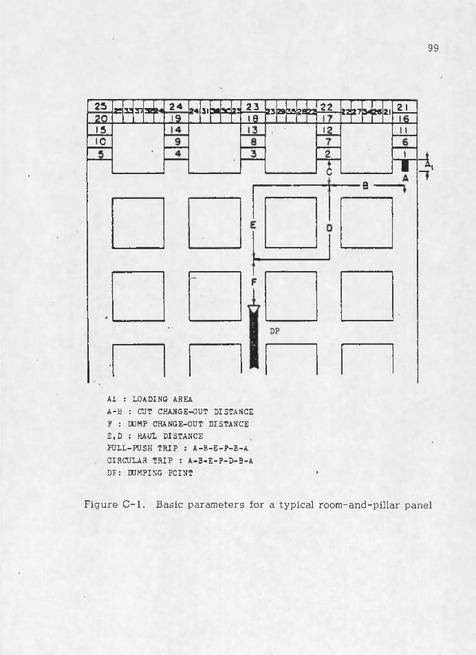
99
252 0
ZS 33 3 1 3 8 6 2419
31M3C2 , 2 218
23 2 9 3 5 2 8 2 2 -— — 8 2 2 7 M W 21225
21
111C
12 11
I n l r i i
B
Ai : LOADING AREA
A -E : CUT CHANGE-OUT DISTANCE
P : DUMP CHANGE-OUT DISTANCE
E ,D : HAUL DISTANCEFULL-PUSH T R IP i A - B - E - P - B - A
CIRCULAR T R IP : A - B - E - P - D - B - A
DP: DUMPING POINT
Figure C - l . Basic parameters for a typical room-and-pillar panel
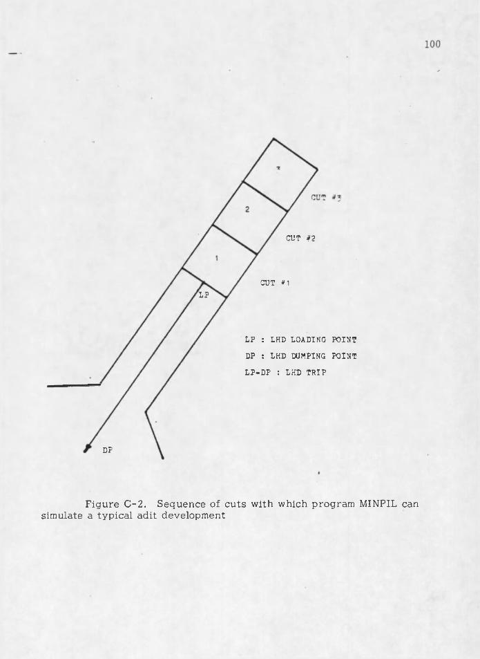
CUT #2
CUT #1
I P
LP : LHD LOADING POINT
DP : LHD DUMPING POINT
L P -D P : LHD T R IP
DP
Figure C-2. Sequence of cuts with which program MINPIL can simulate a typical adit development

1 0 1
CUT #1
CUT *2
L ? : u r n LOADING POINT
DP : LHD DUMPING POINT
L P -D P : LHD T R IP
DP
Figure C-3. Sequence of cuts with which program MINPIL can simulate a typical pile removal
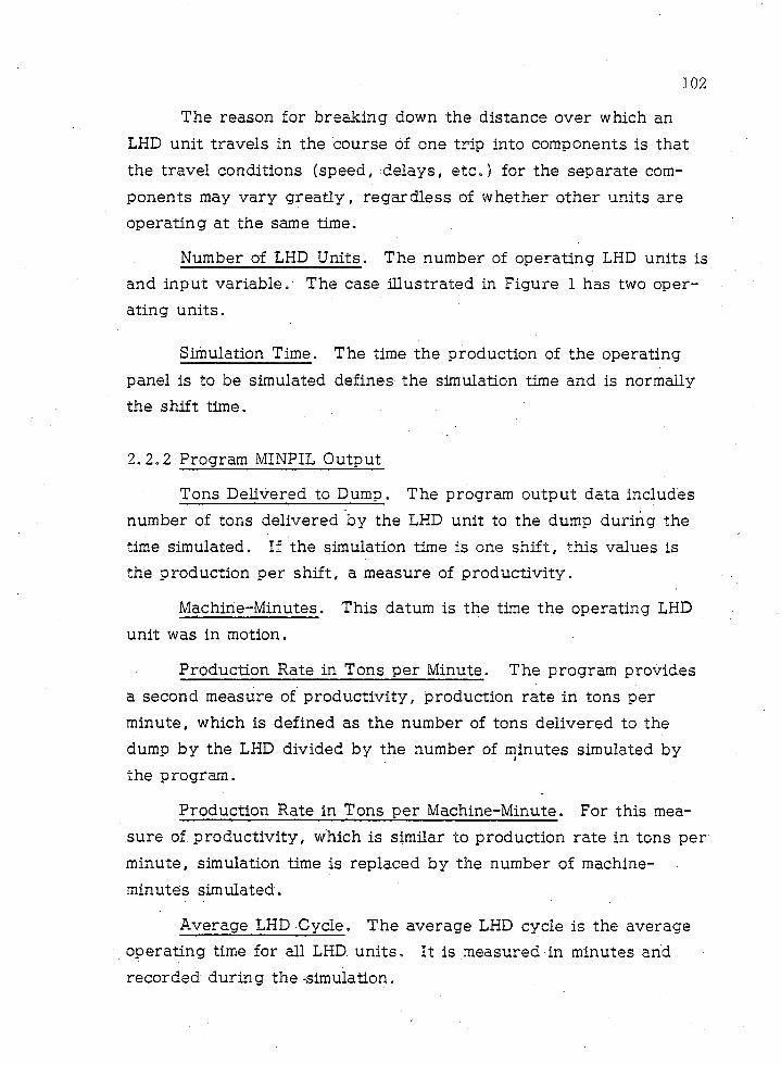
102
The reason for breaking down the distance over which an LHD unit travels in the course of one trip into components is that the travel conditions (speed, delays, e t c .) for the separate components may vary greatly , regardless of whether other units are operating at the same time.
Number of LHD Units. The number of operating LHD units is and input variable. The case illustrated in Figure 1 has two operating units.
Simulation Time. The time the production of the operating panel is to be simulated defines the simulation time and is normally the shift time.
2 .2 .2 Program MINPIL Output
Tons Delivered to Dump. The program output data includes number of tons delivered by the LHD unit to the dump during the time simulated. If the simulation time is one sh ift, this values is the production per shift, a measure of productivity.
Machine-Minutes. This datum is the time the operating LHD unit was in motion.
Production Rate in Tons per Minute. The program provides a second measure of productivity, production rate in tons per minute, which is defined as the number of tons delivered to the dump by the LHD divided by the number of minutes simulated by the program.
Production Rate in Tons per Machine-Minute. For this measure of productivity, which is similar to production rate in tons per minute, simulation time is replaced by the number of machine- minutes simulated.
Average LHD Cycle. The average LHD cycle is the average operating time for all LHD units. It is measured in minutes and recorded during the-simulation.
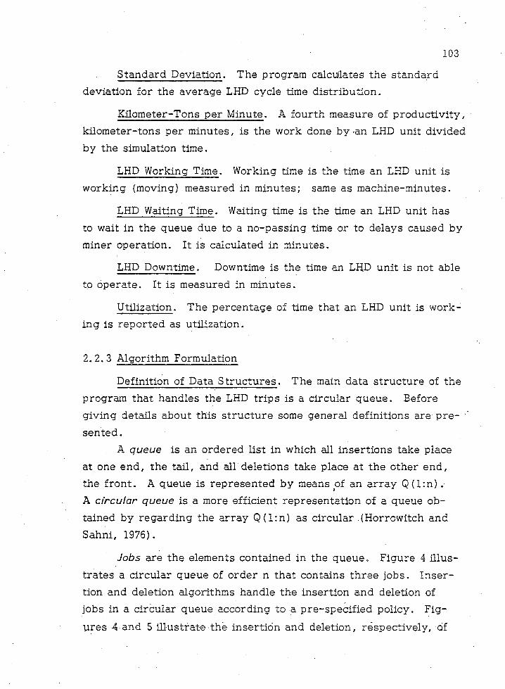
103
Standard Deviation. The program calculates the standard deviation for the average LHD cycle time distribution.
Kilometer-Tons per Minute. A fourth measure of productivity, kilometer-tons per minutes, is the work done by an LHD unit divided by the simulation time.
LHD Working Time. Working time is the time an LHD unit is working (moving) measured in minutes; same as machine-minutes.
LHD Waiting Time. Waiting time is the time an LHD unit has to wait in the queue due to a no-passing time or to delays caused by miner operation. It is calculated in minutes.
LHD Downtime. Downtime is the time an LHD unit is not able to operate. It is measured in minutes.
Utilization. The percentage of time that an LHD unit is working is reported as utilization.
2. 2. 3 Algorithm Formulation
Definition of Data Structures. The main data structure of the program that handles the LHD trips is a circular queue. Before giving details about this structure some general definitions are pre- •' sented.
A queue is an ordered list in which all insertions take place at one end, the tail, and air deletions take place at the other end, the front. A queue is represented by means of an array Q (1:n ) .•A circular queue is a more efficient representation of a queue obtained by regarding the array Q (l:n ) as circular (Horrowitch and Sahni, 1976).
Jobs are the elements contained in the queue. Figure 4 illustrates a circular queue of order n that contains three jobs. Insertion and deletion algorithms handle the insertion and deletion of jobs in a circular queue according to a pre-specified policy. Figures 4-and 5 illustrate the insertion and deletion, respectively, of

104
?RONT
TAIL
FRCMT TAIL
Figure C-4. Insertion of job D in the circular queue
(Q)
FRONT TAILTAIL
FRONT
Figure C-5. Deletion of job A in the circular queue
105
jobs under the policy used in program MINPIL. This policy provides aa counterclockwise development for the queue.
The main advantage of a circular queue over the conventional linear queue is a more efficient use of memory space. A circular queue is developed in a pre-specified set of n memory locations, whereas the required dimension of Array Q cannot be pre-specified or efficiently predicted for a conventional linear, queue because of the insertions and deletions involved.
Circular Queue. The jobs of the circular queue used in program MINPIL are the LHD units. The following steps describe the queue operation and are illustrated in Figure 6.
1. The LHD unit at the front of the queue is deleted and its availability checked by the method that will be described later.
2. If the unit is labeled available it is loaded at the operating cut, sent from the cut to the dumping point, and then returned from the dumping point to the current operating cut. All variables in the program that simulate the trip are updated. When the unit returns to the operating cut, it is inserted at the tail of the queue
3. If the unit is labeled unavailable, it is inserted directly at the end of the queue. The critical event in the circular queue operations is the time the unit is checked for availability. This control takes place before the unit is to be loaded.
Trip Time. A typical LHD trip comprises four activities: . loading, tramming, dumping, and queueing, which program MINPIL simulates. The time for these four activities 'are calculated in the following manner.
1. Loading time. After the LHD has been labeled available, the unit proceeds to the loading area and is loaded in time LT. The loading operation may start at once when the unit enters the cutor it may be delayed due to the performance of the miner. Program MINPIL determines and records the delay time (DEL).
2. Tramming time. After being loaded, the unit trams to the dumping point and then returns to the operating cut. Program

106
DUMPING POINT
LOADING POINT
0 : LOADED LHD UNIT GOING TO THE DUMP
Q : EMPTY LHD UNIT GOING TO THE OPERATIONAL CUT
q : LHD UNIT BEING LOADED
@ : LHD UNIT WAITING TO BE LOADED
0 : LHD UNIT CALLED AND POUND UNAVAILABLE
Figure C-6. Circular queue of program MINPIL with its LHD job
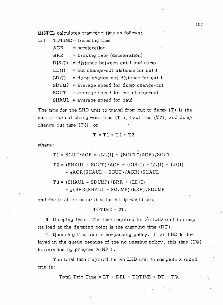
107
MINPIL calculates tramming time as follows:Let TOTIME = tramming time
ACR = acceleration BRR = braking rate (deceleration)DIS(I) = distance between cut I and dump LL (I) = cut change-out distance for cut I LD (I) = dump change-out distance for cut I SDUMP = average speed for dump change-out SCUT = average speed for cut change-out SHAUL = average speed for haul
The time for the LED unit to travel from cut to dump (T) is the sum of the cut change-out time (T l) , haul time (T 2), and dump change-out time (T3), or
T = T l + T2 + T3
where:
T l = SCUT/ACR = (LL(I) - £SCUT2/ACR)/SCUT
T2 = (SHAUL - SCUT)/ACR = (DIS(I) - LL(I) - LD(I)- ^ACR(SHAUL - SCUT)/ACR)/SHAUL
T3 = (SHAUL - SDUMP) /BRR + (LD(I)- i (BRR (SHAUL - SDUMP) /BRR) /SDUMP
and the total tramming time for a trip would be:.
TOTIME = 2T.
3. Dumping time. The time required for an LED unit to dump its load at the dumping point is the dumping time (DT).
4. Queueing time due to no-passing policy. If an LHD is delayed in the queue because of the no-passing policy, this time (TQ)is recorded by program MINPIL.
The total time required for an LHD unit to complete a round trip is:
Total Trip Time = LT + DEL + TOTIME + DT + TQ.

108
Miner Activity. If a continuous miner is incorporated in the mining operation, program MINPIL performs the following task s:
1. Determines if the miner has mined enough material at the time the available LHD unit is ready for loading. If the material is adequate, the unit is loaded. If not, the time the unit has to wait for the material to be mined (PQ) is recorded.
2. Determines if the loading area is occupied by another unit.If it is not occupied, the program performs step 1. If it is occupied the program forces the unit to wait until the area is free, records the time the unit must wait until the other unit is loaded (SQ), and then performs step 1.
3. Calculates the time the unit has to wait in the loading area before loading activities begin (DEL) as
DEL = PQ + SQand records DEL.
Queueing Time Due to No-passing Policy. A delay in the LHD trip caused by the no-passing policy is examined and the delay time (TQ) recorded. The delay time is found by comparing the arrival time in the loading area for the unit under consideration (TARIV)with the arrival time of the last unit called and found available before the arrival of the unit under consideration (T'ARIV).
If TARIV > T'ARIV, TQ = 0
If TARIV < T'ARIV, TQ f 0 = T'ARIV - TARIV
Mechanical Availability. The mechanical.availability of an LHD unit (AV) is defined as
1 ~ AV=BREAKDOWN FREQUENC Y
The task of labeling an LHD unit available or unavailable is performed by a randomizing method, which works according to the following Steps:
1. A random decimal number RN is called.2. It is specified that RN be smaller or larger than AV.

109
3. If RN _< AV, the unit is labeled available; if RN > AV, the unit is labeled unavailable. Figure 7 illustrates the method and gives two examples.
LHP Downtime. The time an LHD unit is down (DW) is recorded by the program. The steps with which the program works are:
1. The time LHD unit I is called and found unavailable (CLN (I)) is recorded.
2. The time LHD unit I is called again and found available (DCL) is also recorded.
3. The program calculates the total downtime for unit I as the sum of the downtimes for that unit, or
DW = Z(DCL - CLN (I))
2.2.4 Simulation Philosophy
The simulation philosophy used .in program MINPIL is event oriented; that is , the state of the system remains constant until the next event is reached (Kim, 1975). In the program, the event occur whenever one of the following conditions are met:
1. The LHD is called and found unavailable.2. The LHD is called and found available.3. The LHD loading is completed.4. The LHD returns to the operating cut.5. The LHD is ready for loading.
When one of these conditions occurs the individual LHD time variables as well as the simulation clock variable are updated. When the simulation clock reaches the amount of time for which the sy stem is to be simulated, the simulation stops and the proper output is generated.
2 .2 .5 Program Constants
Program MINPIL uses the English system with one exception: kilometer-tons per minute as one measure of LHD productivity.

0 . .1 .2 . 3 . 4 .5 .6 ,7 .3 . 9 1 .AVAIXA313 * U NA7AILA3L3
IN PUT A VA ILA BU iITY : 0
CALL2D HANDOM NUMBER :
LEU UNIT : AVAILABLE
INPUT A V A ILA B ILITY : 0
CALLED RANDOM NUMBER :
LED UNIT : UNAVAILABLE
7
.4 5 6
7
.3 9 0
Figure 0 7 , Method by which program MINFIL examines availability of the called unit ,
I l l
2. 3 Program Capabilities
2. 3.1 Deterministic Simulatibn
The program is capable of performing deterministic simulation by using multiple runs and changing the value of a specific variable to be studied. The variables that can be changed are LHD availability, continuous miner availability, distance between the first cut in the sequence and the dumping point, average LHD haul speed, LHD heaped capacity, and cut tonnage. The results of the multiple runs are output by program MINPIL as horizontal histograms that show the impact of the changes of the particular variable on the production recorded at the dumping point.
2 .3 .2 Range of Variables
Due to present dimensioning of the variables, the program can handle no more than 10 LHD units working at the same face and no more than 60 cuts in a sequence cycle.
2 .3 .3 Limitations and Restrictions of Method of Analysis
Certain assumptions incorporated in the model development may affect the accuracy of the program. However, they do not impose serious limitations on program application. The most important limitations and restrictions are:
1. All LHD units discharge at the same point, which is considered the dumping point for the simulated area.
2 . Average speed limits and loading and dumping times were obtained from time studies and were as the mean of their distributions. Field studies show that these values are acceptable.
3. Change-out distances are the same for all operating LHD units.
4. The distance from a particular cut to the dumping point is the same for all LHD units.

112
5. It is assumed that a small tonnage of ore can be stored for a time at the face.
6 . It is assumed that all the mass of a cut is concentrated at its center of mass.
7. All recorded distances are based on measurement from the center lines of the covered drifts and crosscuts.
8 . The program cannot handle LHD dispatching; that is , the program needs a prespecified number of LHD units assigned to the working miner or the working face*of the simulated area.
9. If pull-push LHD trips are incorporated in the program, queueing time is not recorded because of the no-passing policy.The reason for the assumption is that in a pull-push trip environment, each LHD has its own route from the cut to the dumping point and queueing time in the drifts does not exist.
10. In the conventional mining method option of the program, where a continuous miner is not used, it is assumed that loading and tramming operations take place continuously and cannot be interrupted by an other face operation.
1 1 . Both in the conventional and continuous methods, the mine bolter or any other support unit is outside the boundaries of the simulation.
2.3.4 Program Sensitivity
The results of the program are highly sensitive to the availability of the operation LHD units. Sample runs illustrate a case where the best-fit line of the function for LHD availability-resulting production has a slope of 55 degrees (Fig. 8) . This mean that a diference of x% in the correct value for LHD availability in the input data results in an 0.73 x x% in calculated production (tan (90° - 55°) . = 0.73).
In addition to LHD availability, the program is highly sensitive to two other variables: average LHD haul speed and total LHD struck capcity. Best-fit lines for both functions plotted against production have a slope of 65 degrees, which means that a difference

113
L-HO AVAILABILITY
9
c$y^ ? e # e e e c e e a$ c
50 e o o a o e e e e o s e e n ^ e o c g e o
coo ec eo eoa oee eo Qpc o#
O sj r o o e e t : * g g g e o # nxf tf.
a9oa<% a a a e o o e a * # #
30 * 9 c e o o # o # o o * # v***#*#3*###3**o** a #goaoo*
20 9## a#a*#*# 0 3 3 3 # o o 3*######*
10 # # * # # #*#***## ## ###### 4»# #**# 3##3 + 3 #3#33#3# a###*#### 0 . 2 50 . 5 0 0 . 7 5 0 . . 1000,
TONS DELIVERED IN THE 0U*P
Figure C -8 . Typical histogram showing relationship between LHP availability and production per shift

114
of x% in the input data would result in an 0.45 x x% difference in the calculated production. Figure 9 shows a sample histogram that illustrates the relationship between haul speed and production.
An examination of the influence of the availability of the continuous miner on production shows that production is not sensitive to this variable. The best-fit line for this case has a slope of 78 degrees and a difference of x% in the availability of the continuous miner would result in 0 . 22 x x% difference in the production of the LHD unit. Figure 10 illustrates with a histogram the effect of miner availability on LHD production.
2. 3.5 Handling Varied Operating Characteristics
Program MINPIL can solve a variety of problems associated with the operation of LHD units. These problems can be divided into two categories: (1) problems concerning room-and-pillar mining methods and (2) problems arising in general applications of LHD equipment.
■1. Room-and-Pillar Mine Layout Problems. For a specific set of equipment it is often desired to find the optimum cut sequence and cut dimensions for a particular room-and-pillar panel. By using the multiple-runs option of the program and changing the cut dimensions or cut sequence for each run, program MINPIL can determine the optimum layout.
Another problem may be to determine the optimum set of equipment to work in a prespecified panel. Xgain, by using the multiple-runs option and changing the number or characteristics of the LHD units in the set or the characteristics of the miner for each run, program MINPIL can provide information for the optimum equipment selection. It is also possible to simulate the current panel layout with use of the current set of equipment by using the first option of the multiple-runs option.

AVERAGE LHD SPEED
0pO O P O P P P P P P P P P P P O P P P P P P P P P O P P P
5 0 0 o GO P o o o p p c^o q o o o p o p o o o o p p o o o p p p o oO O P O O p o p p O O P P O P P O P P P O O P O P P O P P 0 0O O P P O P P O O O O O O O O O p p O P P O P p p O P
4 5 0 o 0 0 O O O O O O O O O O O O O O O O O O O O O O O O O O P O O P P O P P O P P O P p p p o o p p p p p p p p p p 0 pp p p P O P p p p p o p p p p p p p p p p p p p p p p
^ OO o O O O O O O O O O O O O O O O O O O O O O O O O O O O O P p p p P O P p p p p p p p p p O O P P P P P P P P P P 0 op p p p p p p p p p p p p p p p p p p p p p p p
B 5 0 o 0 0 p o o o o p p p P P P P O P O o o o o o o o o o ^O O P p p p p p p p p p p p p P P P P P P O P P 0 op p p p p p p p p p p p p p p Ppp pp ppp
3 0 0 o 0 0 ' p o p o o o o o o o o o o o o o o o o o o o op p p p p p p p p p p p p p p p p p P O P p p 0 0O O P O O P O O P O O P O O O P P O P O P P
2 5 0 o 0 0 p o p p p p p p p p p p p p p p p p p p p pp p p p p p p p p p p p p p p OOOOOOO O 0p p p p p p p p p - O P P P P P P P P P
2 9 0 o 0 0 o o p p p p p p p p p p p p p p o p p
O O P p p p P O P P P P P P P P P P P 0 oO P O p p p p p p p p p p p p o
1 5 0 o 0 0 p o p p p p p p p p o o p p o op p p p p p p p p p p p p p p P 0 0p p p O O P P P P g o e
1 0 0 o 0 0 o o p p p p p p p p p p
OOP OpOOO 0 PP 0 0 0OOP PPPP »
5 0 0 0 0 o o o o o o oP O O p p p pp o o O O P O O P <>0 0 000 0 0 0 0 4 . O O P o o o o o o < > 0 0 0 0 0 0 0 0 0 ^
Oo 2 5 0 . 5 0 0 . 7 5 0 . 1 0 0 0 ,
TONS DELIVERED IN THE DUMP
Figure C-9. Typical histogram showing relationship between LHD haul speed and production per shift
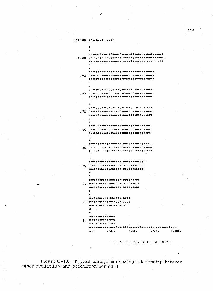
116
HI Nck
1 . 0 0
o bO
o 70
. bO
• :0
« 30
oiO
0 10
AVAILABIL ITY
»o9#$ *o$ ****** *$000*0***
9 * * 9**099 $ 0* 00 * 0**00 * * * * 00 * 0 0 0 0 * 0 ** * * * 0 * 0 * 0 * * o o * # * o * * * * * o * * o o * o * * * * o **oo* 0*0 0 00 OOOOOO 00**00*0**009**
*** 0*0*0*oo**** **0**000*******
*** *********00* *00*0*******0*0
*
0 * 0 * * * * * * * * * * * * 0 * 0 OooO* OOOOoO*0*0 **oo* * *o* * * * O* **00*0**00*0
*** ************ **************
o 4$OO* ** 0*0* 0*0 0** ** o * * * 0*00*00*
*** ***o*o $***** *************** * * * * 00*0 * 000*0 * 0*0 000 * 00 0 0 0 *
**** ************ oO*0**0******
090 900**0 90*90* OO*0*0000*000
*** ************ *o<%*00*0**00<i
**0*0 OOOOOOoo0*0* O* 0*0000000*0*
OO* **O»0*0**00********000*0**
0*0 *0*00* ****** 0*0**00**0000*
ao0*0*0**0**0*000*0*00*0*0$
* o******* ****** oOOo******
*** *$*Oo* $$00*0 00*00*0*0*
9** * * 0 * 0 o * * 0 * * 0 o * o o * * * * * *$*0*0*$**$0*0 0*oo***o*$
*00*0**0000*00***0*****
o **0*00**00*0$*****$$
o o * 0 * * 9 0 * 0 0 9 * 0 0 o o * ** $* 00$ *00 *0**0 0 00*0
* 1
cOO*Oo***opoo
* ** 0 0 * 0 * 0 o o **0*0*0*0*00*
0*0 OOOOO* «.*0000 00 0 * 000***0*04. *oo$o**o*<»
0 . 2 5 0 . 5 0 0 . 7 5 0 . 1 0 0 0 .
TONS DELIVERED. I,S THE CUM?
Figure C -10 . Typical histogram showing relationship between miner availability and production per shift

The program is capable of performing sensitivity analyses to determine the effect of any of the input variables.on production.One variable from a specified set of variables can be changed in each run of the second option of the multiple-runs options to show its impact on production.
Program MINPIL is able to handle circular or pull-push LHD trips in a simulated room-and-pillar panel. The program is also able to simulate room-and-pillar methods incorporating continuous miners (continuous method) or the conventional mine cycle (conventional method). ^
2. General LHD applications. Program MINPIL is able to simulate LHD operations in tunnel development work by treating it as a special case of the room-and-pillar procedure in which the cuts to mined and hauled form the shape of the tunnel.
Several mining methods require LHD units to load and haul a quantity of material from a loading point not at the face to another point. By considering the point at which the material is concentrated (loading point) as a production face, the program is able to incorporate this operation. A similar problem, the removal of a pile of material from one loading point to another point or to a draw point, is treated in the same way.
Data Inputs- v " v
2.4.1 Introduction
The data are input from punched cards or from a disk file that use a pre-specified format. The following pages illustrate by card type the data needed in the program. All data are contained on 16 card types. The user is cautioned to be consistent in the use-of units throughout input.
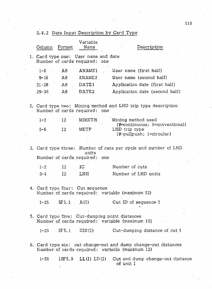
2.4 .2 Data Input Description by Card Type
Column FormatVariable
Name Description
Card type one: User name and dateNumber of cards required: one
1-8 A8 ANAME1 User name (first half)9-16 A8 ZNAME2 User name (second half)
21-28 A8 . DATE 1 Application date (first half)29-36 A8 DATE 2 Application date (second half)
Card type two: Mining method and LHD trip type description Number of cards required: one
1-2 12 MIMETH Mining method used(0=continuous; 1 conventional)
5-6 12 METP LHD trip type(0-pullpush; l=circular)
Card type three: Number of cuts per cycle and number of LHDunits
Number of cards required: one
1-2 12 IC Number of cuts3-4 12 LNH Number of LHD units
Cut sequencerequired: variable (maximum 12)
A (I) Cut ID of sequence I
Card type five: Cut-dumping point distances Number of cards required: variable (maximum 12)
1-25 5F5.1 DIS(I) Cut-dumping distance of cut I
Card type six: cut change-out and dump change-cut distancesNumber of cards required: variable (maximum 12)
1-50 10F5.0 LL(I) LD(I) Cut and dump change-out distanceof unit I
Card type four: Number of cards
1-25 5F5.1
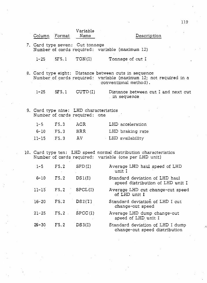
119
VariableColumn Format Name Description
7. Card type seven : Cut tonnageNumber of cards required: variable (maximum 12)
1-25 5F5.1 TON (I) Tonnage of cut I
8 . Card type eight: Distance between cuts in sequenceNumber of cards required: variable (maximum 12; not required in a
conventional method).
1-25 5F5.1 CUTD(I) Distance between cut I and next cut. in sequence
9. Card type nine: LHD characteristics Number of cards required: one. ■
1-5 F5.3 ACR LHD acceleration6 -10 F5.3 BRR LHD braking rate
11-15 F5.3 AV ■ LHD availability
Card type ten: LHD speed normal distribution characteristics Number of cards required: variable (one per LHD unit)
1-5 F5.2 SPD(I) Average LHD haul speed of LHD unit I
6 -1 0 F5.2 DSl(I) Standard deviation of LHD haul speed distribution of LHD unit I
11-15 F5.2 : SPCL (I) Average LHD cut change-cut speed of LHD unit I
16-20 F5.2 DS2(T) Standard deviation of LHD I cut change-out speed
21-25 F5.2 SPCC(I) Average LHD dump change-out speed of LHD unit I
26-30 F5.2 DS3(D Standard deviation of LHD I dump change-out speed distribution
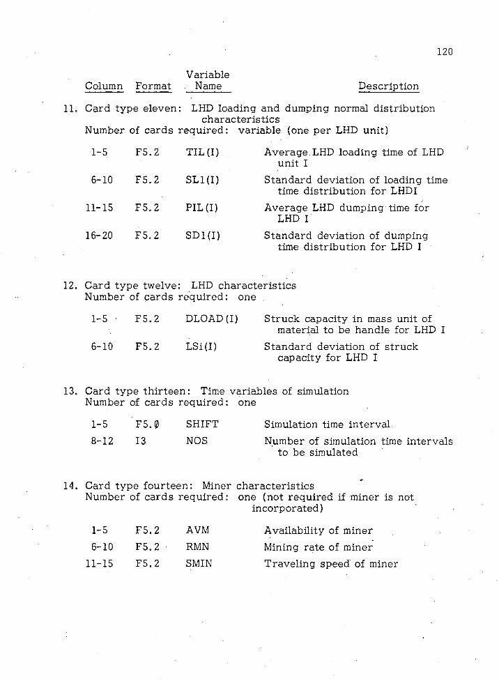
Column FormatVariable . Name Description
Card type eleven: LED loading and dumping normal distributioncharacteristics
Number of cards required: variable (one per LED unit)
1-5 F5.2 TIL (I) Average LED loading time of LED unit I
6-10 F5.2 SL1(I) Standard deviation of loading time time distribution for LEDI
11-15 F5.2 PIL(I) Average LED dumping time for LED I
16-20 F5.2 SD1(I) Standard deviation of dumping time distribution for LED I •
Card type twelve: LED characteristics Number of cards required: one
1-5 • F5.2 DLOAD(I) Struck capacity in mass unit ofmaterial to be handle for LED I
6-10 F5.2 LSI (I) Standard deviation of struck capacity for LED I
Card type thirteen: Time variables of simulation Number of cards required: one
1-5 F5. 0 SEIFT Simulation time interval8 -1 2 13 NOS Number of simulation time intervals
to be simulated
Card type fourteen: Miner characteristicsNumber of cards required: one (not required if miner is not
incorporated)
1-5 F5.2 AVM Availability of miner6 -10 F5.2 RMN Mining rate of miner
11-15 F5.2 SMIN Traveling speed of miner

121
VariableColumn Format Name Description
15. Card type fifteen : Variable to be change in multiple runs Number of cards required: one
1-2 12 NES Code of variable to be changed inmultiple runs
(0 = no variable to be changed1 = LHD availability2 = miner availability3 = first cut-dump distance4 = LHD average haul speed5 = total LHD capacity6 = cut tonnage)
16. Card type six teen : switchesNumber of cards required: one
1 -2 12 LSW1 Multiple-runs control switch (0 = no multiple runs required
1 = multiple runs required-5-6 12 LSW2 Number of card to be read for next
run if LSW1 = 1 (99 - last run)9-10 12 LSW3 Input data printout control switch
(0 = No; 1 = Yes)13-14 12 LSW4' Histogram requirement control
switch if LSW1 = 1 (0 = No; 1 = Yes)
17-18 12 NRUN Number of present run (1-10)
Figure 11 shows an 80-80 listing of data card types 1 through 16 for a simulation study of two sh ifts.
2.5 Program Options
The program has several options that are controlled by switches and variables. A discussion of these options follows:
2 .5 .1 Multiple Runs.The user can make single or multiple runs with program
MINPIL. The options of the multiple-runs applications are:

1 2 2
001 0 MAZARIS GEORGE 2 / 3 / 3 1 CARD TYPE 1
002 0 1 1 CARD TYPE 2
0 0 3 0 20 1 CARD TYPE 3
004Q 1 O 2 - 3 . 4 o 5 . CARO TYPE 4
0 0 5 0 6 c 7 o 8 c 9c 1 0 c CARD TYPE 4
0 0 6 0 1 1 O 1 2 , 13 o 1 4 . 1 5 . CARD TYPE 4
0 0 7 0 1 6 o 1 7 o 1 8 , 1 9 , 2 0 . CARD TYPE 4
OOSO 21 Do 2 1 0 , 2 1 0 c 2 1 0 , 2 1 0 . CARD TYPE 5
0 0 9 0 2 1 0 c 21 0 o 2 1 0 . 2 1 0 . 2 1 0 , CARD TYPE 5
01 0 0 2 1 0 c 2 1 0 c 210 o 2 1 0 c 2 1 0 , CARD TYPE 5
Q U O 2 1 0 c 210 c 210 o 2 1 0 , 2 1 0 . CARD TYPE 5
0 12 0 0 c Oo Oc Oc Oc Oc Oo Oc Oc Oo CARD TYPE 6
0 1 3 0 Oc Oc Oc Oc 0 . Oc Oo Oo Oc Oc CARO TYPE 6
0 1 4 0 Oc Oo Oc Oo Oc Oc Oo 0 o Oo Oo CARD TYPE 6
0 1 5 0 Oo Oc Oo Oo Oc Oc Oo Oo Oc Oo CARD TYPE 6
0 16 0 4 1 , 8 41c 8 4 1 . 8 4 1 . 8 41 o 8 CARD TYPE 7
0 1 7 0 ■9* e— Co 4 1 , 8 41 c 8 4 1 . 3 4 1 . 8 CARD TYPE 7
0 1 8 0 41 c 8 4 1 c 8 4 1 . 8 4 1 . 8 41 . 8 CARD TYPE 7
0 1 9 0 41 08 4 1 . 6 4 1 c 8 4 1 , 3 41 o,3 CARD TYPE 7
0 2 0 0 3 6 2 0c 3 6 2 0 o 0 o 9 7 CARD TYPE 9
0 2 1 0 33 4 o Oo Oo Oo Oo Oo CARD TYPE K
0 2 2 0 Oo 69 Oo Oo 4 2 Oo CARD TYPE 1
0 2 3 0 4c 0 0 CARD t y p e .1
0 2 4 0 448o 2 CARD TYPE 1
0250 0 CARD TYPE 1
0 260 0 0 C 0 1 CARD TYPE 1
Figure C - ll . Sample input data for a two-shift simulation study

123
1. To perform a simulation study for more than one pre-specified simulation time interval.
2. To perform a simulation study changing the value of a specific variable in each run.
The first option of the program (multiple simulation time operation) is performed automatically by the program and controlled by variables SHIFT and NOS. As has been described, SHIFT defines the simulation time and NOS the number of time intervals to be simulated. For example, if two sh ifts, 400 minutes each, are to be simulated, the variables SHIFT and NOS must take on the following values:
SHIFT = 400.NOS = 2
Figure 11 illustrates a complete input data printout for the simulation of two 400-minute sh ifts.
The second option of the program, deterministic simulation by changing values of a variable in each run, is more complex and is controlled by the available switches and variables. The following elements must be considered before applying multiple-runs option 2 .
1 . All data required by the program are read only in the first run and need not be read in the following runs unless they change.
2. Except for the first run, where all input data are required, every subsequent run must includ two data types:
a. The data card type that includes the variable to bechanged.
b. Data card type 16, which includes the switches.3. The variable to be changed is defined in the first run.
Having presented general information about the application of multiple-runs option II, a detailed step-by-step description of this operation follows.
Step 1 : The user must initialize the following variables in the first run of a multiple-runs option II.

124
a. NES = { 1 ,2 ,3 ,4 ,5 ,6 }. As had been mentioned, the variable NES defines the variable to be changed from the following run.
NES = 1: the changing variable is LHD availabilityNES = 2: the changing variable is miner availabilityNES = 3: the changing variable is first cu-dump
distanceNES = 4: the changing variable is LHD average load
speedNES = 5: the changing variable is total LHD capacityNES = 6 : the changing variable is cut tonnage
b. LSW1 = 1: this switch initiates multiple-runs option IIc. LSW2 = {3 ,4 ,5 , . . . , 15}: this switch defines the card
type to be read in the following run. Because the program is able to handle changes in only one variable, switch LSW2 must have the same number in all runs.
d. Switch LSW4 is not activated in the first run and can take any value.
Step 2: For each additional run switches LSW1 and LSW2 must take on the same values as in run 1. Variable NRUN must have the number of the present run. • Switch LSW4 is not activated.
Step 3: For the last run the following must be done:a. LSW1 = 1 : value of this switch does not changeb. LSW2 = 99: shows that the present run is the last run
to be donec. LSW4 = {0,1}: defines if a histogram is required
(1:Yes; 0:No)d. The variable NRUN must take on the number of the
present run (which is the last one).
As an illustration of the application of multiple-runs option II, suppose that the user wants to perform a sensitivity analysis with the following characteristics:
1 . The LHD availability is to be changed six times (10%-60% with with an interval of 10%).

126
UOulO000200 0 0 3 00 0 0 4 00 0 0 5 00 0 0 6 00 0 0 7 00 0 0 6 00 0 0 9 0001000 0 1 1 0001200 0 1 3 00014 00 0 1 5 0
hAZ APIS GEURGc 2 1
3 0 2 1.6 a
1 / 2 0 / 3 1
2 e 3 o 4 o 5 o7 o do 9 o 10 o
1 1 . 12 o 13 o 1 4 © 15 o1 6 o 17 « 1 b o 1 v • 20#21# 22# 23# 24 , 25#2 o# 27 o 2 8 , 2 9 , 30#
600# oOO o oOO# 600# 70 0#7 0 Co 700# 700# 800# 800#800# 800 # 900 # 900# 900#90 0# 1000 o1 0 0 0 # 1 0 0 0 # 1 0 0 0 #
110 0#1100 #1 1 0 0 # 1100# 1 2 0 0 # 1230# 1200 #1200# 1300# 1300#
0 0 1 6 0 30# 30 # 30# 30#0 0 1 7 0 30# 30 # 30# 30#0 0 1 5 0 3 o# 30 # 30 # 30 #U O 1 9 0 3 v« 30 # . 30# 30#0 0 2 0 0 3 0 # 30 # 3 0 # 30#0 0 2 1 0 30# 3 0 # 30# 30#0 0 2 2 0 1 0 0 # 1 0 0 # 1 0 0 # 1 0 0 #0 0 2 3 0 1 0 0 # 1 0 0 # 1 0 0 # 1 0 0 #0 0 2 4 0 1 0 0 # 1 0 0 # 1 0 0 # 1 0 0 #oO 25.0 1 0 0 # 1 0 0 # 1 0 0 , 1 0 0 #U 0 2 6 0 U O # 1 0 0 # 1 0 0 # 1 0 0 #U 0 2 7 0 1 0 0 # ICO# 1 0 0 # 1 0 0 #0 0 2 8 0 1 0 0 # 100'# 1 0 0 # 1 0 0 #0 0 2 9 0 1 0 0 # 1 0 0 # ICO# 3 3 0 #0 0 3 0 0 1 3 6 # 1 3 6 # 3 4 2 # 1 4 6 #vO.310 1 4 6 # 3 4 8 # 1 4 8 # 12#0 0 3 2 0 1 2 # 1 4 8 # 2 4 3 # 24#u 0 3 j 0 6 6# 6 6 # 66# 6 6 #0 0 3 4 0 3 5 2 0 # 35 20 # #1U 0 3 5 0 4 4 0 # 10 # 3 5 0 # 10 #003o0 4 4 0 # 10 # 3 5 0 # 1 0 ,0 0 3 7 0 #5 #0 5 #5 #0 50 0 3 8 00 0 3 9 00 U 4 0 00 0 4 1 0
#57,7#
4 0 0 #
# 0 5 » 5 # 5
1
#5 #05
0 0 4 2 00 0 4 3 0
#61
b # 1 0 0 #
0 0 4 4 0 1 9 1 0 10 0 4 50 3 5 2 0 # 3 5 2 0 # #20 0 4 6 0 1 9 1 0 2U 0 4 7 0 . 3 52 0# 3 5 2 0 # #30 0 4 8 0 1 9 1 0 30 0 4 9 0 3 5 2 0# 3 5 2 0 # # 40 0 5 0 0 1 9 1 0 40 0 6 1 0 3 5 2 0# 3 5 2 0 # #50 0 5 2 0 1 9 1 0 50 0 5 3 0 3 5 2 0 # 3 5 2 0 # #60 0 5 4 0 1 9 9 1 1 6
30# 30# 30 # 3 0 . 3030# 30# 30# 3 0 , 3 030 # 3 0# 3 0 # 3 0 # 3030# 30# 30 # 3 0 , 303 0 , 30# 30# 3 0 , 3030# 30# 30# 30# 30
1 0 0 #
100#1 0 0 ,1 0 0 #
1 0 0 #
1 0 0 #
3 1 2 #1 3 6 #1 4 b #1 4 8 #
2 4 #
1 0 #
1 0 #
1 # 1 -
CARO TYPE 1CARO TYPE 2CARD TYPE 3CARO TYPE 4CARO TYPE 4CARO TYPE 4CARO TYPE 4CARO TYPE 4CARD TYPE .4CARD TYPE 5CARD TYPE 5CARD TYPE 5CARD TYPE 5CARO TYRE 5CARO 1 Y=E 5
» CARD TYPE 6# CARD TYPE 6, CARD TYRE 6» CARD TYPE 6, CARO TYPE 6» CARD TYPE 6
CARD TYPE .7CARD TYPE 7CARO TYPE 7CARD TYPE 7CARD TYPE 7CARO TYPE 7CARO TYPE 8CARO TYPE 8CARO TYPE 8CARO TYPE 8CARD TYPE bCARO TYRE 8CARO TYPE 9CARD TYPE 10CARO TYPE 10CARD TYPE 11
. CARO TYRE 11CARD TYPE 12CARD TYPE 1 2CARD TY3 E 13CARD TYPE 14CARD TYPE 15CARD TYPE 16CARD TYPE 9CARD TYPE 16
~ CARO TYPE 9CARD TYPE 16CARO TYPE 9CARO TYPE I dCARD TYPE 9CARO TYPE 16
. CARD TYRE 9CARD TYPE 16
Figure C -12. Sample input for an LHD availability sensitivity analysis

127
1 . Single runThe available output is a simulation report for this run.
. 2. Multiple runsa. Option I (multiple simulation time generation)
The available outputs are a simulation report for each run and a general simulation report at the end of the last run.
b. Option II (sensitivity analysis)The available outputs are simulation reports at the end of
each run and, if requested, a horizontal histogram illustrating the results of the runs.
The program generates an input data list (echo check), which is available for each run and option.
Figure 13 shows the program out put for single run and Figure 14 shows the histogram from multiple-runs option II (input shown in Figure 12 ) .
The structure of a simulation report is divided into the main parts:1 . Production Summary.
a. Tons deliver to the dump.b. Machine-minutes simulated..^c. Production rate in tons/minute.d. Production rate in tons /machine-minute
2 . Haulage Summarya. Average LED cycle.b. Standard deviation of LED cycle time distribution.c. Production rate in kilometer-tons per minute.
3. Wait Time Analysisa. Working time per LED unit.b. Waiting time per LED unit.c. Downtime per LED unit.d. Utilization per LED unit.
2.7 Other Outputs
None.

128
S H I F T
P R O D U C T I O N S U M M A R Y
TO'i S DELIVERED TO THE DUMP
MACHINE MINUTES SIMULATED
PRODUCTION RATE IN TONS PER MINUTE
PRODUCTION RATE IN TONS PER MACHINE MINUTE
4 0 8 . 0 0 0
2 1 7 . 4 6 6
2 . 0 4 0
1 . 8 7 6
HAULAGE S UMMARY
AVERAGE LHO CYCLE
STANDARD DEVIATION
PRODUCTION RATE IN KILOMETER TONS/ MIN
2 . 1 5 5
.222
2 6 . 6 3 6
W A I T T I M E A N A L Y S I S
LrtO UNIT WORKING TIME WAITING TIME DOWN TIME UTI LIZATION PRC LOAD HAULED
1 1 1 2 . 9 9 7 0 . 0 0 0 8 2 . 6 4 0LrtO UNIT WORKING TIME WAITING TIME DOWN TIME
i 0 4 o 4 09 2 . 1 3 2 92 o 399
56© 498 UTILIZATION PRC
5 2 o 2 3 4
212 o 000LOAD HAULED
19 6 o000
Figure 0 1 3 . Sample output for a single run
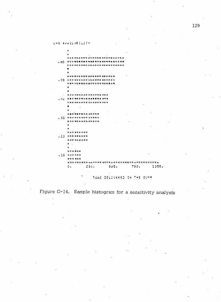
129
11 o
Figure C
A~li.ll ABILITY
:0
j? o -p 93?999 * 9 9 9 9 9 9 * 9 9 9 99 9 9*999 9 9 99 9 9 9 0 9 9 999 99 9 999999 9*9 9 9 * * 9 9 * 9 9 9 9 9 * 9 9 * 9 *
9
999 9 99999 999 99 9 99*
4(J $*9 6 9 9 * 9 9 9 * 9 * * * * 9 *0 9* * 0 * 99 9 9 9 9 9 9 9 0 9 *
*
30 9 9 0 0 * 0 0 0 9 9 * 0 9 9
* 9 * * 9 * * 9 * *9* *9
20
10
*0 9 90*09*
* 9 * ** * « * *
9 0 9 O** * 9 *
*
90 9 * * 9 99 0* 0 * 090* *9*
0 9* *9 9 9 9 O
Go 2 50. 5 0 0 , 7 5 0 , 1 3 0 0 .
T0,\S DELIVERED IN T ’ E O'J*?
-14. Sample histogram for a sensitivity analysis

130
2 . 8 Flow Chart
• See Figure 15.
2.9 Sample Runs
See Figures 16, 17, 18.

131
^ : START
READ DATA
WRITE DATA
CALL INPUT
W rite o u t in p u t da ta
CALL CRQUEUE
Manage LHD c i r c u la r queue
CALL AVAIL
Check i f c a l le d u n i t is a v a ila b le
isthe LHD
a v a ila b le
YES
th e re any queue v
YES
LHD t r i p p u ll-p u s h .
C a lc u la te queue tim e
Check f o r t r i p queueing
CALL CYCLE
E s ta b lis h th e one-way t r a v e l t im e
CALL TOTCYC
E s ta b lis h the t o t a l t r i p tim e
he LHD goes’ to th e dump and re tu rn s to c u t
CALL NORM
E s ta b lis h the dum ping, lo a d in g tim es and speeds
Figure C-15. Flowchart for program MINPIL

132
CALL EXCAV
Check f o r de la ys due to m in e r
FIND TIME LHD HAS TO WAIT
FOR MINER
ISTHE SHIFT FINISHE
PRINT SHIFT RESULTS
CALL OUTPUT
P r in t o u t s h i f t r e s u lts
^ HAVE x THE SHIFTS ^F IN IS H E D ,
YES
READ DATA FOR
NEXT RUNTHIS THE LASIp X . RUN /
YES
I PRINT SIMULATION
REPORTHISTOGRAMREQUEST
YES
CALL PLTINT
P r in t o u t the h is to g ra m
CALL OUTPUT
P r in t o u t the s im u la t io n re p o r t
PRINTHISTOGRAM
END
Figure C~ 15—-Continued
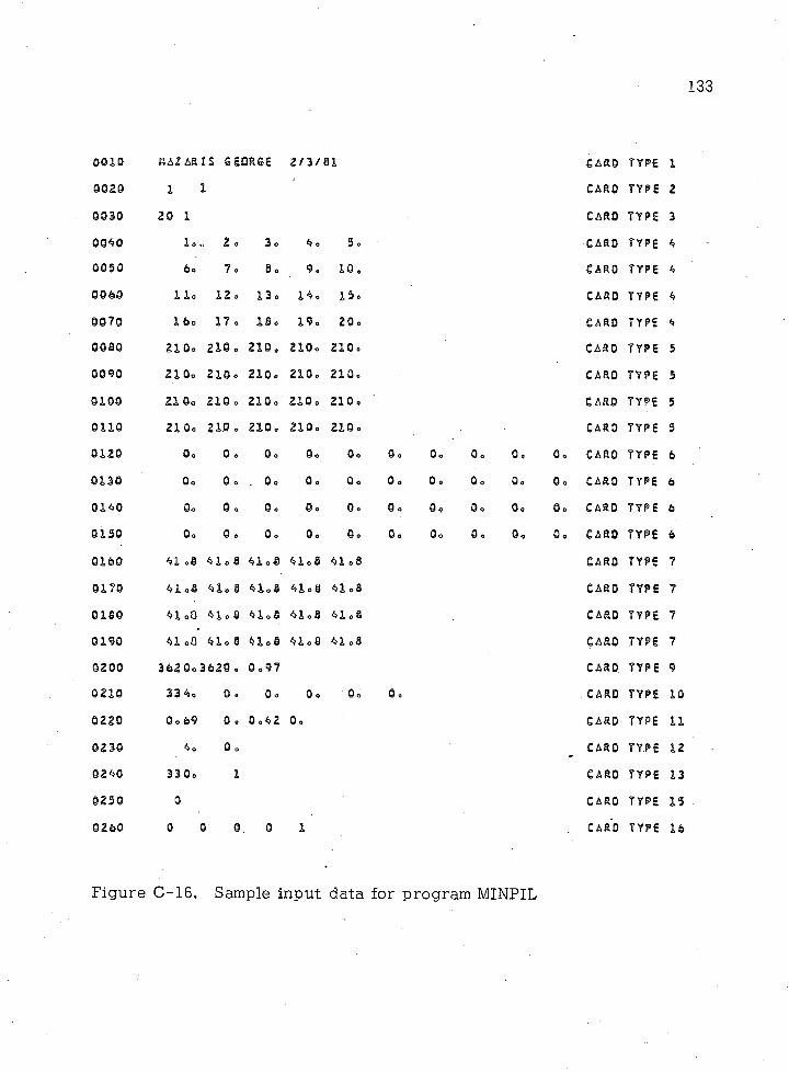
133
0010 BAZAR IS GEORGE 2 / 3 / 8 1
0020 1 10 0 3 0 2 0 1
0 0 4 0 l o „ 2 . 3 . 4 . 5 o
0 0 5 0 6o 7 o 8. 9 o 1 0 .
9 0 6 0 l i o 12 o 1 3 . 1 4 o 13 o
9 0 7 0 1 6o 1 7 o 1 8 . 1 9 . 20,
o o a o 21 Oo 210 o 210 o 210. 210.
0 0 9 0 2 1 Do 210. 210. 2 1 0 . 210o
0100 2 1 Oo 2 1 0 . 2 1 0 . 210. 2 1 0 .
0110 2 1 0 . 210 o 210. 2 1 0 . 210 o
0 1 2 0 Oo Oo 0. 0. 0 .
0 1 3 0 0. 0 0 . 0 . 0. 0 o
0 1 4 0 Oo 0 0 Oo 0. Oo
0 1 5 0 Oo 0 o 0 . 0 . Oo
0 1 6 0 4 1 . 8 4 1 . 6 4 1 . 8 4 1 . 8 4 1 . 8
0 1 7 0 4 1 . 8 4 1 . 8 4 1 . 8 4 1 . 8 4 1 . 8
0 1 8 0 4 1 . 0 4 1 . 8 4 1 . 8 4 1 . 8 4 1 . 8
0 1 9 0 41 oO 4 1 . 8 4 1 . 8 4 1 . 8 4 1 . 8
0200 3 6 2 Oo 3 6 2 0 o 0 . 9 7
0 2 1 0 3 3 4 . 0 0 Oo Oo 0.
0 2 2 0 0 . 6 9 0 0 0 , 4 2 0.
0 2 3 0 4 . Oo
0 2 4 0 3 3 0 . 10 2 5 0 00260 0 0 0 0 1
0 A R 0 TYPE 1
CARO TYPE 2
CARD TYPE 3
CARO t y p e 4
CARD TYPE 4
CARO TYPE 4
CARO TYPE 4
CARO TYPE 5
CARO TYPE 5
CARD TYPE 5
CARD TYPE 5
0 , Oo Oo Oo Oo CARD TYPE 6
0 . 0 . 0 . Oo Oo CARO TYPE 6
Oo Oo Oo 0 . 0 . CARD TYPE 6
0 . Oo Oo 0 . 0 . CARD TYPE 6
CARO TYPE 7
CARO TYPE 7
CARD TYPE 7
CARO TYPE 7
CARO. TYPE 9
CARO TYPE 10
CARO TYPE 1 1
CARO TYPE 12
CARO TYPE 1 3
CARO TYPE 1 5
CARO TYPE l b
Figure C-16. Sample input data for program MINPIL

134
S H I F T 1
P R O D U C T I O N S U M M A R Y
Tj NS DELIVERED TO THE DUMP 5 7 2 . 0 0 0
MACHINE MINUTES SIMULATED 3 0 4 . 3 7 8
PRODUCTION KATE IN TONS PER MINUTE 1 . 7 3 3
PRODUCTION RATE IN TONS PER MACHINE MINUTE 1 . 8 7 6
HAUL AGE S UMMARY
AV eRAGc LHO CYCLE 2 . 1 3 2
STANDARD d e v i a t i o n . 0 0 0
p r o d u c t i o n r a t e ' i n k i l o m e t e r t o n s / m i n - 3 1 . 7 2 9
d A I T T I M E A N A L Y S I S
LriJ U N I T ' WORKING TIME WAITING TIME DOWN TIME UTI LI ZATI ON PRC
1 3 0 4 . 8 7 8 0 . 0 0 0 2 5 . 0 0 0 9 2 . 3 8 7
Figure C -17. Sample output data from program MINPIL
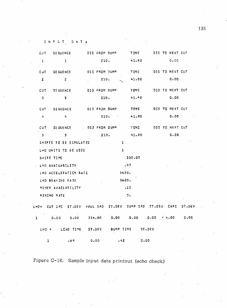
135
I N P U T D A T a
CUT SEQUENCE DIS FROM DUM*
1 1 210 o
CUT SEQUENCE DIS FROM DUMP
2 2 210 o
CUT SEQUENCE DIS FROM DUMP
3 3 210o
CUT SEQUENCE DIS FROM DUMP
4 4 2 1 0 o
CUT SEQUENCE DI S FROM DUMP
5 5 210oSHIFTS TO BE SIMULATED
LHD UNI TS TO BE USED
SHIFT TIME
I HD AVAILABILI TY
LHD ACCELERATION RATE
LHD BRAKING RATE
MINER AVAILABILITY
MINING RATE
LHD* CUT 5PD ST, DEV HAUL SPD
1 0 , 0 0 0 , 0 0 3 3 4 , 0 0
LHD o LOAD TIME ST, DEV
1 ,69 0,00
TONS DIS TO NEXT CUT
4 1 . 9 0 0 , 0 0
TONS DIS TO NEXT CUT
4 1 . 8 0 0 , 0 0
TONS DIS TO NEXT CUT
41.90 0,00
TONS DIS TO NEXT CUT
4 1 . 8 0 0 , 0 0
TONS DIS TO NEXT CUT
4 1 . 8 0 C,CO
1
1
3 3 0 , 0 0
, 9 7
3 6 2 0 ,
3 6 2 0 ,
, 10
5 ,
ST, DEV DUMP SPD ST, DEV CAPC ST,
0 , 0 0 0 , 0 0 0 , 0 0 - 4 , 0 0 0 ,
DUMP TIME ST, DEV
, 4 2 0 , 0 0
DEV
00
Figure 0 1 8 . Sample input data printout (echo check)

136
SECTION 3
SYSTEM DOCUMENTATION
3. 1 Computer Equipment
The program was run on the CDC 6400 computer at The University of Arizona using a 110K central memory core.
3. 2 Peripheral Equipment
The following peripheral equipment was used in executing the program: a CDC 512 line printer
3.3 Source Program
A listing of the source program is given in Exhibit B .
3.4 Variables and Subroutines
The following is a list and brief descriptions of the program's subroutines in the order of their occurrence:
CRQUEUG: manages the LED circular queue.AVAIL: checks the availability of the called unit.NORM: generates values following the standard normal distri
bution.TOTCYC: calculates the one-way LHD trip, including loading and
dumping time.CYCLE: calculates the one-way travel time of an LHD unit.STATIS: calculates the mean and standard deviation of a
distribution.OUTPUT: prints out the simulation reportEXCAV: examines the activities of a continuous miner excavation
and reports possible delays caused by it.INPUT: prints out the input data.HIS TO: plots the histograms

PLTINT: initializes the array to be plotted.
For a list of the program variables see Exhibit A.
3.5 Storage Requirements/
As presently structured, program MINPIL requires approximately 11 OK storage on the CDC 6400.
3. 6 Maintenance and Updates
None to date.

138
SECTION 4 ;
OPERATING DOCUMENTATION
4.1 Operating Instructions
Program MINPIL is operated under the CDC 6400 operating system.
4.2 Operating Messages
Normal system messages are produced.
4.3 Control Cards
Program MINPIL can be executed with standard SCOPE 3.4 control cards. As run on the University of Arizona CDC 6400, the makeup of the input deck is:
FTN.LGO.7 /8 /9<SOURCEPROGRAM>7 /8 /9<INPUT DATA>677/8 /9
4.4 Error Recovery
Standard operating actions are required.
4. 5 Run Time
The total run time depends on the number of runs made, the number of LHDs available, the number of cuts to be simulated, and the simulation time. In general, the program needs two (2) seconds

compilation time and about two (2) seconds for every run made after the compilation on the CDC 6400

140
A(I)
EXHIBIT A
LIST OF MAJOR VARIABLES IN PROGRAM MINPIL
Cut ID of sequence IACR Acceleration of LHD unitsAV Availability of LHD unitsAYM • Availability of continuous minerBRR Braking rate of LHD unitsCLN(I) Last time LHD unit I was called and found unavailableCLOCK (I) Clock variable which determines time status of LHD unit ICTON Tonnage delivered to dump during a set of runs .CUTD(I) Distance between cut I and next cut in mining sequenceDATE! Program application date (first half)DATE-2 Program application date (second half)DCL Time last LHD unit arrived at cutDCLOCK (I) Time LHD unit I arrived at cutDEL Time of delay due to continuous minerDIS(I) Distance between cut I and dumpDLOAD(I) Struck capacity of LHD unit IDMN Ore tonnage left in cut after LHD unit is loadedDS Total distance covered by all operating LHD units in one runDS1(I) Standard deviation of haul speed distribution for LHD unit IDS2(I) Standard deviation of cut change-out speed distribution for
DS3(I)LHD unit I " >
Standard deviation of dump change-out speed distribution for
DSTLHD unit I
Total distance covered by all operating LHD units during a
DWset of runs
Recorded part of downtime of an LHD unitITY Used input datai . e . Number of cuts in a panel cycleLCLOCK (I) Time LHD unit I leaves operating cut after having been loaded

LD (I) Dump change-out distance of cut ILHD(I) Defines if called LED unit I is available or unavailableLHDCL(I) Total time LED unit I was working during a runLEDCO Total time all operating LED units were working during a runLEDWT(I) Total time LED unit I was waiting during a runLK Flag which shows if the continuous miner has to move to next
cut in sequenceLL(I) Cut change-out distance of cut ILNE Number of operating LED unitsLPR Used output unitLSW1 Switch which defines requirement of multiple-runs option bLSW2 Switch which defines card type to be read in next runLSW3 Switch which defines if an input data printout is requiredLSW4 Switch which defines if a horizontal histogram is required,
after multiple runs of option IILT Loading time of an LED unitMETP Defines type of LED trips (circular or pull-push)MIMETE Defines type of mining method (continuous or conventional)NES Code of variable to be changed during a multiple-runs deter
ministic simulationNOS Number of time intervals to be simulatedNRUN Number of the run in operationORE Ore extracted by miner during the time between departure of
one LED unit and the arrival of the next unitPL Payload hauled by an LED unit during a tripPR (I) Utilization for LED unit IPRT1 Production rate in tons per minutePRT2 Production rate in tons per machine-minutePRT3 Production rate in kilometer-tons per minutePRTY(I) Downtime of LED unit IRCL Time loading of last LED unit startedRCLOCK(I) Time loading of-LED I startedREM Excavated ore remaining at operating face after an LED unit
has been loadedRMN Excavation rate Of minerRN Random number called

142
SCUT Cut change-out speed of an LED unitSDUMP Dump change-out speed of an LED unitSEN (NI) Value of variable to be change in multiple runs at run NISEAUL Eaul speed of an LED unitSEIFT Time interval of the simulationSL Time miner is ready to start operation after an LED unit's
departure or after tramming to next cut in sequenceSLS Departure time of last LED unit from operating faceSMIN Tramming speed of minerSNAY(NRUN) Availability value of an LED unit at run NRUNSNAVM (NRUN) Availability value of miner at run NRUNSNLB (NRUN) Total LED struck capacity at run NRUNSNSP(NRUN) Value of average LED haul speed at run NRUNSNT (NRUN) Tons delivered to dumping point at end of run NRUNSNTON (NRUN) Mean of cut tonnage used in run NRUN
Mean of dump change-out speed distribution, for LED unit IMean of cut-change-out speed, distribution! for LED unit IMean of haul speed distribution for LED unit ITime an LED unit has to wait before it proceeds to the miner
because loading area is occupied by another unitTons delivered to the dump from the operating cut during a
runTons delivered to the dump during a runTrip time from time an LED unit leaves the operating cut to
time it reaches the dumping pointTotal cycle time for an LED unit tripTime needed by an LED unti to cover the dump change-out
distanceTime needed by an LED unit to cover the haul distanceTime needed by an LED unit to cover the cut change-out
distanceWaiting time during a run for LED unit I Downtime during a set of runs for LED unit I Tonnage of Cut ITotal excavated material stored at operating face when an .
LED unit arrives
SPCC(I)SPCL(I)SPD(I)SQ
STN
STONT
TIMETIM1
TIM 2 TIMS
TLEDT(I) TLWN(I) TON (I) TORE

TOTIME Time, including dumping and loading time, for a one-way LHD trip
TPR Time continuous miner is free (time between arrival of an LHD unit and time preceding LHD unit departed)
TPRM Actual working time of a continuous miner due to its availability
TQ Queueing time of an LHD unit during a tripTWN(I) Total downtime of LHD unit I during a runZNAME1 User name (first half)ZNAME2 User name (second half)

EXHIBIT B
SOURCE PROGRAM LISTING OF MINPIL

145
000100 0 0 2 00 00 3000 04 00 0 0 5 000 0 6 000 0 7 00 0 08 00 0 0 9 000100001100012000 13 000 1 4 000 1 5 00 0 1 6 00 0 1 7 00 0 1 8 00 0 19 000200002100022000 23 00 024 00 0 2 5 0002600 0 2 7 000 2 8 00 0 2 9 00 03 000 0 3 1 00 03 2000 3 3 00 03 400 03 500 0 3 6 00 0 3 7 00 0 3 8 00 0 3 9 000 4 0 00 04 1 00 04 2000 4 3 00 04 4000 4 5 00 04 6 00 0 4 7 000 4 8 00 0 4 9 0U05G00 05 100 0 5 2 00 0 5 3 000 54 000 5 5 00 0 5 6 00 0 5 7 00 0 5 8 00 0 5 9000 6 0 00 0 6 1 0
C PROGRAM .NINPIL5D6C 1 0 jGoMoMAZARIS2OCTOBER 19 8 0 C DEPARTMENT OF MINING AND GEOLOGICAL ENGINEERING,C UNIVERSITY OF ARIZONA, TUCSON ARIZONA*
PROGRAM MXNPIL(INPUT, OUTPUT,TAP£ 5 ° INPUT,TAPE6°0UTPUT)
C• 0**000*0000*0***0*0*00*0*********************00**0**********
C PROGRAM DESCRIPTIONC THIS PROGRAM SIMULATES THE LOAD-HAUL-OUMP ACTIVITYC . OF AN UNDERGROUND MINE WHEN LOAO-HAUL-OUMP C UNITS ARE USED
C THE PROGRAM IS COMPOSED OF ONE MAIN PROGRAM AND ELEVENC SUBROUTINES tilCH PERFORM AN EVENT ORIENTED SIMULATION
C THE PROGRAM USES THE DETERMINISTIC AND THE STOCHASTIC APPROACH.C THE STOCHASTIS VARIABLES INCLUDE THE LHO LOAD AND DUMP TIME,C THE LHO DUMP CHANGE-OUT,CUT CHANGE-OUT, HAUL SPEEDC AND THE EXACT PAYLOAD
C EVERY CUT THAT IS MINED IS DEFINED BY ITS SEQUENCE,ITSC DISTANCE FROM THE DUMPING POINT,ITS DISTANCE FROM THE NEXTC CUT IN SEQUENCE AND ITS TONNAGE.
C THE PROGRAM CAN HANDLE CONVENTIONAL OR CONTINOUSC MINING METHODS AS WELL AS CIRCULAR OR PULL-PUSH LHOC TRIPS
C POSSIBLE QUEUEING OR BREAK-DOWN TIMES IN THE LHOC OPERATION, WHICH CAN BE CAUSED BY ELEMENTS WITHIN THEC SIMULATION BOUNDARIES,ARE ALSO CONSIDERED
COMMON A, IG, OIS , TON, CUTD, NOS, LNH, SHIFT, AV, ACR, 8RR,1 AVM, RMN, SPCL, DS2, SPO, DS1, SPCC, DS3, DLQAO, L S I ,T I L ,S M I2 , S L 1 , PIL, SOI , LPR, ITYCOMMON ZNAME1, ZNAME2, 0ATE1, 0ATE2, MIMETH, METP,ISt i l , L5ti2,1 LSW3, LSU4, NRUN, NESr e a l l e i o c k , 8 d, Ihde 1, I h d e o , I h d wt , M , 1 o a d , 1 t , mn REAL MAXHDIMENSION A ( 6 0 ) , C U T D ( 6 0 ) p 0 I S ( 6 0 ) , L D ( 6 0 ) , L L ( 6 0 ) , T 0 N ( 6 0 )DIMENSION 0 L Q A 0 ( 1 0 ) , D S l ( 1 0 ) , 0 S 2 ( i 0 ) , 0 S 3 ( 1 0 ) , L S l ( 1 0 ) , P I L ( 1 0 ) ,1 S D K 1 0 ) , S L 1 ( 1 0 ) , S P C C ( 1 0 ) , S P C L ( 1 0 ) , S P O ( 1 0 ) , T I L ( 1 0 )
o * o * * o o * * * * * o o * 0 * INPUT DATA DESCRIPTION o * * * ^ * * * * * * * * * * * * * * * *
COL
CARD 11 -8 9e 17 2 0 - 2 8 2 9 - 3 9 .
CARD 2 1 -2
FORMATa a oo o o o
NAMEo a o o o
DESCRIPTIONo o o a a a a a o a o
USER NAME AND DATEA8 ZNAME1A8 ZNAME 2A8 DATE1A8 DATE2
USER NAME USER NAME DATE DATE
DESCRIPTION OF METHOD AND LHD TRIP TYPE12 MIMETH MINING METHOD
^CONVENTIONAL0°C0NTINU0US

1460 0 6 2 00 0 6 3 0 C 5 - 6 12 METP LHD TP IF TYPE0 0 6 4 0 C ^CIRCULAR0 0 6 5 0 C 0°PULL—PUSH0 0 6 6 0 c0 0 6 7 0 c CARO 3 SIMULATION CUTS AND NO QtF LHD UNITS0 0 6 8 0 c 1 - 2 12 IC NO OF CUTS00 6 9 0 c 3 - 4 12 LNH NO OF LHD UNITS0 0 7 0 0 c0 0 7 1 0 c CARD 4 CUT SEQUENCE0 07 20 c 1 - 2 5 5P5 o 1 A d ) CUT ID OF SEQUENCE X0 0 7 3 0 c0 0 7 4 0 c CARD 5 CUT-OUMP DISTANCES0 0 7 5 0 c 1 - 2 5 5F5 o 1 D I S m CUT-OUMP DISTANCE OF CUT I0 07 60 c00 77 0 c CARD 6 CUT- AND DUMP-CHANGE-OUT DISTANCES0 0 7 8 0 c 1 - 5 0 10F 5o0 I L ( X ) p L O ( I ) CUT AND DUMP CHANGE-OUT0 0 7 9 0 c DISTANCE OF CUT I0 0 8 0 0 c0 0 8 1 0 c CARD 7 CUT TONNAGE00 8 2 0 c 1 - 2 5 5 F 5 o l TON C I ) TONNAGE OF CUT I0 0 8 3 0 c0 0 8 4 0 c CARO 8 DISTANCE BETWEEN CUTS IN SEQUENCE0 0 8 5 0 c 1 - 2 5 5F5 o1 CUTDCX) DISTANCE BETWEEN CUT I00 8 6 0 c AND THE NEXT CUT IN SEQUENCE0 0 8 7 0 c0 0 8 8 0 c CARO 9 LHD CHARACTARI#STXC50 0 8 9 0 c 1 - 5 F5o3 ACR LHD ACCELERATION0 0 9 0 0 c 6 - 1 0 F5»3 BRR LHD BRAKING RATE0 0 9 1 0 c 1 1 - 1 5 F5 o 3 AV LHD AVAILABILITY0 0 9 2 0 c0 09 30 c CARD 10 LHD SPEED OISTXBUTXQN CHARACTERISTICS0 0 9 4 0 c 1 - 5 ‘ F5o2 S P O (I ) I UNIT AVERAGE HAUL SPEED0 09 50 c 6 - 1 0 F5o2 D S 1 ( I ) I UNIT HAUL SPEED SToOEVXATX0 0 9 6 0 c 1 1 - 1 5 F5o 2 SPCL(I ) I UNIT AVERAGE CUT00 9 7 0 c CHANGE-OUT SPEED0 09 8 0 c 1 6 - 2 0 F5 o 2 DS23CI) I UNIT CUT CHANGE-OUT0 0 9 9 0 c SPEED STo DEVIATION0 1 0 0 0 c 2 1 - 2 5 F5o2 SPCC(I) I UNIT AVERAGE DUMP010 10 c CHANGE-OUT SPEED0 1 0 2 0 c 2 6 - 3 0 F5o2 DS3( X) I UNIT DUMP CHANGE-0103 0 c OUT SPEED STo DEVIATION01 04 0 c0 10 5 0 c CARD 11 LHD CHARACTERISTICS0 1 0 6 0 c 1 - 5 F5o2 T I L ( I ) X UNIT AVERAGE LOADING TIME0 1 0 7 0 c 6 - 1 0 F5o 2 S L l ( I ) UNIT I LOADING01 0 8 0 c TIME STo DEVIATION0 1 0 9 0 c 1 1 - 1 5 F5o2 P X L d ) I UNIT AVERAGE DUMPING TIME0 1 1 0 0 c 1 6 - 2 0 F5o2 so im UNIT I DUMPINGOH IO c TIME STo DEVIATION01 1 2 0 c0 1 1 3 0 c CARD 12 LHD CHARACTERISTICS0 1 1 4 0 c 1 - 5 F5o2 DLOADd) I UNIT STACK CAPACITY0 1 1 5 0 c 6 - 1 0 F5 o 2 LSI(X ) I UNIT STRACK CAPACITY0 11 6 0 c STo DEVIATION0 1 1 7 0 c0 1 1 8 0 c CARO 13 TIME VARIABLES OF SIMULATION0 1 1 9 0 c 1 - 5 F5oO SHIFT SHIFT TIME01 2 0 0 c 8 - 1 2 13 NOS NO OF SHIFTS TO BE01 2 1 0 c SIMULATED01 2 2 0 c

147
01 2 3 0 C CARD 14 MINER CHARACTERISTICS0 1 2 4 0 c 1 - 5 F5o2 AVM MINER AVAILABILITY0 1 2 5 0 c 6=10 F5o2 RMN MINING RATE0 1 2 6 0 c 1 1 - 1 5 F5o2 SHIN MINER TRAMMING SPEED0 1 2 7 0 c0 1 2 8 0 C CARO 15 VARIABLE TO BE CHANGED IN MULTIPLE RUNS0 1 2 9 0 c 1 - 2 12 NES CODE OF VARIABLE TO BE CHANGE0 1 3 0 0 c 0°NQ VARIABLE CHANGED0 1 3 1 0 c loLHO AVAILABILITY01 3 2 0 c 2=MINER AVAILABILITY0 1 3 3 0 c 3°FIRST CUT-0UMP DISTANCE0 1 3 4 0 c 4=LH0 AVERAGE HAUL SPEED0 1 3 5 0 c 5°T0TAL LHO CAPACITY0 1 3 6 0 c 6°CUT TONNAGE0 1 3 7 0 c0 1 3 8 0 c CARD 16 SWITCHES0 1 3 9 0 c 1 - 2 1 2 LSti l MULTIPLE RUN CONTROL01 4 0 0 c 0°NO MULTIPLE RUNS0 1 4 1 0 c . loMULTIPLE RUNS RE9UIRED0 1 4 2 0 c 5—6 12 LSW2 CARD ID TO BE READ FOR NEXT0 1 4 3 0 c (99°LAST RUN)0 1 4 4 0 c 0r-01
1 2 LSW3 INPUT DATA PRINT-OUT0 1 4 5 0 e 1°YES0 1 4 6 0 c 0=NO0 1 4 7 0 C . 1 3 - 1 4 1 2 LSW4 HISTOGRAM RE9UIRMENT0 14 8 0 c 0°N00 1 4 9 0 c 1°YES0 1 5 0 0 c 1 7 - 1 8 1 2 NRUM NO OF PRESENT R U N ( l - l O )0 1 5 1 0 c.0 1 5 2 0 LPR=60 1 5 3 0 ITY°50 1 5 4 0 e0 1 5 5 0 c OOOO0 0 0 0 * 0 0 0 0 0 0 0 0 0 0 * 0 OOOOOOOOOOOOOOOOOOOOOOOOOOOOOOOOOOOOOOO0 1 5 6 0 c — -READ THE INPUT DATA0 1 5 7 0 c # 0 0 0 0 0 0 0 * 0 0 0 0 0 0 0 0 0 0 0 0 0 0 0 * 0 0 0 0 0 0 0 * 0 0 0 0 0 0 0 0 0 0 0 0 0 0 0 0 0 0 0 0 0 0 0 0 0 0 00 1 5 8 0 e0 1 5 9 0 c0 1 6 0 0 c — -CARD TYPE 10 1 6 1 0 c0 1 6 2 0 10 REAOCITY si 2 0 0 0 ) ZNaHEIoZNAME OATElj)0 ATE20 1 6 3 0 c0 1 6 4 0 c—-CARD TYPE 20 1 6 5 0 c0 1 6 6 0 RE AO ( ITY » 202.0) niMETHpflETP0 1 6 7 0 c '0 16 8 0 c—-CARD TYPE 30 1 6 9 0 c0 1 7 0 0 20 RE AD < ITY » 2 0 2 0 ) ICj> LNH0 1 7 1 0 IF (NRFUNoGEo2.) GO TO 1 8 00 1 7 2 0 C -0 1 7 3 0 c ~ -CARO TYPE 40 1 7 4 0 c0 1 7 5 0 30 READ( ITY * 2 0 2 5 ) < A < I ) » I ° 1 » I C )01 7 6 0 IF(NRUMo GEol ) GO TO 1800 1 7 7 0 c0 1 7 8 0 c~ -CARD TYPE 50 1 7 9 0 c0 1 8 0 0 40 RE AO ( ITY » 2 0 2 5 ) (DIS ( I )» I ° l » IC )0 1 8 1 0 I F ( N R U N o G E o l ) GO TO 1800 1 8 2 0 C0 1 8 3 0 C—=-CARD TYPE 6

148
0 1 8 4 00 1 8 5 00 1 8 6 00 1 8 7 00 1 8 8 00 1 8 9 00 1 9 0 00 1 9 1 00 1 9 2 00 1 9 3 00 1 9 4 00 1 9 5 00 1 9 6 00 1 9 7 00 1 9 8 00 1 9 9 00200002010020200 2 0 3 00 2 0 4 00 2 0 5 00 2 0 6 00 2 0 7 00 2 0 8 00 2 0 9 00210002110021200 2 1 3 00 2 1 4 00 2 1 5 00 2 1 6 00 2 1 7 00 2 1 8 00 2 1 9 0022000221002220 -
0 2 2 3 00 2 2 4 00 2 2 5 00 2 2 6 00 2 2 7 00 2 2 8 00 2 2 9 00 2 3 0 00 2 3 1 00 2 3 2 00 2 3 3 00 2 3 4 00 2 3 5 00 2 3 6 00 2 3 7 00 2 3 8 00 2 3 9 00 2 4 0 00 2 4 1 00 2 4 2 00 2 4 3 00 2 4 4 0
C5 0
CC—c6 0
a£A D< XT Y/ >20 30 H U U X U U H I ) ) p X ° 1 j>XC) XF (NRUNoGEol ) GO TO 1 8 0
-CARO TYPE 7
R e A 0 ( X T Y p 2 0 2 5 ) ( T Q t m > » X ° X j > X C ) XF(NRUMoGSol ) GO TO 1 8 0
XF(HXMETHoEQol) GO TO 8 0CC —C7 0
CC —C8 0
9 0Cc~=c100
110cc---c120
1 3 0CC-----C
1 4 0
CC ~c1 5 0
Cc™c1 6 0
Cc— c1 7 0CC — C 1 8 0
"CARD TYPE 8
REA0( XTYp 2 0 2 5 ) ( CUTO ( X ) p X n lj>XC) I F ( N R U N o G E o l ) GO TO 1 8 0
-CARO TYPE 9
REAO( XTYp2 0 4 0 ) ACRpBRRpAV XF(NRUNq GEoX) GO TO 1 8 0 00. 100 XolpLNH
-CARO TYPE 10
READCXTYp 2O5O)SPOCX)p 0 S 1 ( X ) pSP CL (X ) pO S 2 ( X ) p SPCC(X)pOS3CX) CONTINUE
IF <NRUN0 G E o l ) GO TO 1 8 0 DO 1 2 0 l * U i m
CARD TYPE 1 1
REA0(XTYp 2 0 5 0 > T X L ( X ) p S L 1 ( X ) p P X L ( X ) p S D I ( X) CONTINUE
XFCNRUNoGEol) GO TO 1 8 0 DO 1 4 0 X ° 1 p LNH
CARD TYPE 12 ■
RE AD C XTYp 2 0 5 0 ) 0 U0A0 C X) p L S I < X)CONTINUE
XF(NRUNo G E o l ) GO TO 1 8 0
►CARD TYPE 13
READC XTYp2 0 6 0 ) SHIFTpNOS I F ( N R U N o G E o l ) GO TO 1 8 0
XF(HXFlETHoEQol) GO TO 1 7 0
CARO TYPE 14
‘ REAO^ XTYp 2 0 5 0 ) AVHp RNNp SHXNXFCNRUNoGEol) GO TO 18 0
CARO TYPE 15
READ(XTYp2 0 7 0 )NES
CARO TYPE 16
READ C XTYp2 0 8 0 )LSt i lpLSt i2pLSk!3pLSt i4pNRUN XF CLSHSo EQoO) GO TO 1 9 0

149
0 2 4 5 0 e0 2 4 6 0 c ™ ° CALL SUBROUTINE INPUT TO PRINT OUT THE INPUT DATA0 2 4 7 0 c OOOOOOOOOOOOCOOOOOOOOQOOiMOOOOOOOOOOOOOOOOOOOOCOOOOOOOOOOOO:)0 2 4 8 0 c0 2 4 9 0 CALL INPUT0 2 5 0 0 c0 2 5 1 0 c ooooooOOOOOO0 0 0 0 * 0 0 0 0 0 0 OOOOOOOOOOOOOOQOOOOOOOOOOOOOOOO0 * 00 2 5 2 0 CALL SUBROUTINE CRQUEUS TO MANAGE THE CIRCULAR QUEUE0 2 5 3 0 C $!)0 0 * 0 * 0 * 0 0 0 0 0 0 0 0 * 0 0 0 0 0 * 0 0 0 0 0 0 0 0 0 0 * 0 0 0 0 0 * * * 0 0 0 0 0 0 * 0 0 0 * o o o o o *0 2 5 4 0 c0 2 5 5 0 1 9 0 CALL CRQUeUE0 2 5 6 0 I F ( L 5 t i 2 o E Q o 9 9 o Q R o L S U 2 o £ Q o O ) GO TO 2 0 00 2 5 7 0 GO TO ( 2 0 0 p 1 0 p 2 0 p 3 0 p 4 0 p 5 0 p 6 0 p 7 0 p 8 0 p 9 0 p 1 1 0 p 1 3 0 p 1 5 0 p 1 6 0 p 1 7 0 ;0 2 5 8 0 1 LSU20 2 5 9 0 2 0 0 STOP0 2 6 0 0 2 0 0 0 FORMAT C4 A 8)0 2 6 1 0 2 0 1 0 FORMAT(I2p 2 X p 1 2 )0 2 6 2 0 2 0 2 0 FQRMATC2I2)0 2 6 3 0 2 0 2 5 FORMAT(5F5o1 )0 2 6 4 0 2 0 3 0 FORMAT(10F5 o O)0 2 6 5 0 2 0 4 0 FORMAT(3 F 5 o 3 )0 2 6 6 0 2 0 5 0 F ORMAT( 6F5o2)0 2 6 7 0 2 0 6 0 FORMAT CF 5o Op 2Xp 1 3 )0 2 6 8 0 2 0 7 0 FORMAT( 1 2 )0 2 6 9 0 2 0 8 0 FORMAT ( X 2 p 2X/ >I2 p 2Xp I 2 p 2Xp I 2 p 2Xp^I2p2X)0 2 7 0 0 END0 2 7 1 00 2 7 2 0 SUBROUTINE CRQUEUE0 2 7 3 0 C0 2 7 4 00 2 7 5 0 C— THIS SUBROUTINE MANAGES THE LHO CIRCULAR QUEUE0 2 7 6 00 2 7 7 0 C 0 0 * 0 0 0 * * 0 * 0 * 0 0 0 * 0 0 * 0 0 0 0 0 0 0 * 0 0 0 0 0 0 0 * 0 0 * 0 0 * 0 0 0 * 0 * 0 0 0 0 0 0 0 * 0 0 * 0 00 2 7 8 0 COMMON Ap ICp OXSp TONp CUTDp NOSp LNHp SHXFTp AVp ACRp BRRp0 2 7 9 0 1 AVHp SMNp SPCLp 0 S 2 p SPOp D S I p SPCCp 9 S 3 p DLOAOp L S I p T I L p SM0 2 8 0 0 2 p S L I p P I L p S D I p LPRp ITT0 2 8 1 0 COMMON ZNAMElp ZNAM£2p OATEIp 0ATE2p MIMETHp METPp LSU I p LSti2p0 2 8 2 0 1 LStiBp LSHAp NRUNp NES0 2 8 3 0 r e a l I e i o c k p I d p I h d e l p I h d c o p 1 hdwfcpI Ip 1o a d p 1 t pmn0 2 8 4 0 REAL MAXH0 2 8 5 0 DIMENSION A C 6 0 I p C L ( 1 0 0 p 1 0 ) p C LO C K( I O )pCUTDC60 ) p0 2 8 6 0 1 DCLOCK( 1 0 ) p OI S C 6 0 ) pLCLOCK( 1 0 ) p L 0 ( 6 0 ) p LH0 ( 1 0 ) p LHOCL( 1 0 ) p0 2 8 7 0 2 L H D U T ( 1 0 ) p L L ( 6 0 ) p L O A D ( 1 0 ) p P R ( 1 0 ) p S T ( 6 0 p 3 0 p I O ) pTLHOL( 1 0 ) p0 2 8 8 0 3 TLHOTC1 0 ) p TO N i 6 0 ) » TUN< 1 0 ) pRCLOCK( 1 0 ) p Z S R ( 1 0 ) ptiORK( 1 0 )0 2 8 9 0 DIMENSION C L N ( 1 0 ) p P R T A < 1 0 ) p S E N ( 1 0 ) p T L t i N ( 1 0 ) p P R l ( 1 0 )0 2 9 0 0 DIMENSION 0 L 0 A 0 ( 1 0 ) p S N A V ( 1 0 ) p SN A V M ( 1 0 ) p S N L B ( 1 0 ) p S N T ( 1 0 ) p0 2 9 1 0 1 SNTONC1 0 )0 2 9 2 0 DIMENSION 0 5 1 ( 1 0 ) p O S 2 ( 1 0 ) p 0 S 3 C 1 0 ) p LS1 ( 1 0 ) p P I L ( 1 0 ) p S O I ( 1 0 ) p0 2 9 3 0 1 S L K 1 0 ) p SNCTO ( 1 0 ) pSMSP( 1 0 ) pSPCC ( 1 0 ) p S P CL ( 1 5 ) pSPO ( 1 0 ) pTIL ( 1 0 )0 2 9 4 0 C0 2 9 5 0 C * t i < n ) * 0 * * * * * * * * * * * * * * * * * * * * * * * * * * * * * * * * * * * * * * * * * * * * * * * * * * * * * *0 2 9 6 0 C----- THE CIRCULAR QUEUE OF THE LHO OPERATION I S MANAGED THROUGH THE0 2 9 7 0 C FOLLOWING A CTI VI TI ES 80 2 9 8 0 C0 2 9 9 0 C ' l o I NI TI ALIZATION OF THE TIME THE UNITS ARRIVE AT THE CUT0 3 0 0 0 c FOR THE FIRST TIME0 3 0 1 0 c0 3 0 2 0 c 2 o UNIT AVAILABILITY CHECK BEFORE IT STARTS GETTING LOADED0 3 0 3 0 c0 3 0 4 0 c 3o UNIT LOADING0 3 0 5 0 e

0 3 0 6 0 C 4o LHO UNIT ROUND TRIP FROM THE CUT TO THE DUMP0 3 0 7 0 00 3 0 8 0 c 5 o CHECK FOR QUEUEING TIME IN THE TRIP0 3 0 9 0 c0 3 1 0 0 e 6o CHECK FOR DELAYS CAUSED BY THE CONTINUOUS MINER0 3 1 1 0 e0 3 1 2 0 c0 3 1 3 0 c0 3 1 4 0 c0 3 1 5 0 C----- ACTIVITY lo0 3 1 6 0 C0 3 1 7 0 c--- ■INITIALIZE THE TIME THE LHO UNITS ARRIVE AT THE CUT0 3 1 8 0 c FOR THE FIRST TIME, AND ZERO THE PRODUCTION VARIABLES0 3 1 9 0 c OOOOgOOOOOOOOOzMzOOOJMCOOOOOOOOOOOiMOOOOOOOOGOOOOOOOOOOO:):)*:):)0 3 2 0 0 c0 3 2 1 0 RCLOCKl l ) ° l o0 3 2 2 0 IF(LNHoEQol) GO TO 200 3 2 3 0 LI°LNH—10 3 2 4 0 DB 10 I ° 1 , L I0 3 2 5 0 RCLOCK <I * 1 ) ° R C L 0 C K ( I )0 3 2 6 0 10 CONTINUE.0 3 2 7 0 20 CTONoOo0 3 2 8 0 STON°Oo0 3 2 9 0 0 0 30 N ° l , I C0 3 3 0 0 00 30 M ° l , 300 3 3 1 0 DO 30 I °1 ,LNH0 3 3 2 0 t iORK(I )°0o0 3 3 3 0 LHOCL(I)°Oo0 3 3 4 0 TLHOL CI ) ° 0 o0 3 3 5 0 LH0CL(I )°O»0 3 3 6 0 30 S T i N o M , I ) ° 0 o0 3 3 7 0 C0 3 3 8 0 c0 3 3 9 0 c— =’■ACTIVITY 2<,0 3 4 0 0 c0 3 4 1 0 c---■THE PRODUCTION STARTS AMO FOLLOtiES THE DEFINED SEQUENCE,0 3 4 2 0 c THE PROGRAM CLOCK IS UPDATED AFTER EVERY ACTIVITY,0 3 4 3 0 c CALL THE LHO UNIT FROM THE HEAD OF THE QUEUE AND USE0 3 4 4 0 c SUBROUTINE AVAIL TO DETERMINE ITS AVAILABILITY, THE0 3 4 5 0 c AVAILABILITY TEST OCCURES BEFORE THE UNIT STARTS GETTING0 3 4 6 0 c LOADED0 3 4 7 0 c OOOOOOCOOOOO OggOOOOOOOOOOOOOgOOWOOOOOOOOOiMOOWOOiXiOOOO#:):)#0 3 4 8 0 DO 210 N o llic03 4 9 0 S T N° 0 ,0 3 5 0 0 DO 200 Md 1 , 300 3 5 1 0 40 BO 150 1 = 1 , LNH0 3 5 2 0 CALL AVAIL(AV,LHO,I)0 3 5 3 0 1 F ( L H D < I ) = l ) 5 0 , 6 0 , 600 3 5 4 0 c0 3 5 5 0 c THE CALLED UNIT 15 UNAVAILABLE, IF THE UNIT WAS UNAVAILABLE0 3 5 6 0 c THE LAST TIME IT WAS CALLED, DO NOT UPDATE THE TIME IT0 3 5 7 0 c STARTED BEING DOWN, IF THE LAST TIME IT WAS CALLED THE UNIT0 3 5 8 0 c WAS AVAILABLE, INITIALIZE THE TIME IT STARTED BEING DOWN0 3 5 9 0 c0 3 6 0 0 c0 3 6 1 0 50 IF(CLN<I)»NE,0)GOTQ 1500 3 6 2 0 CLN(I) °RCLOCK(I)0 3 6 3 0 GOTO 1500 3 6 4 0 c0 36 50 c0 3 6 6 0 c---■THE LHO UNIT IS AVAILABLE, CHECK IF THIS UNIT WAS AVAILABLE
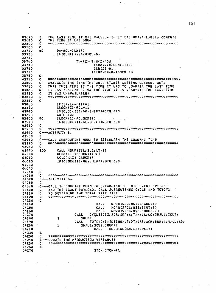
151
0 3 6 7 0 C THE LAST TIME IT WAS GALLED* IF IT WAS UNAVAILABLE, COMPUTE0 36 8 0 C, THE TIME XT WAS DOWN0 3 6 9 0 C o o o o o o o o o o o o o o o o o o o o o o o o o o o o o o o o o o o o o o o o o o o o o o o o o o g o o o o o o o o #0 3 7 0 0 c0 3 7 1 0 60 0 t i= 8C L -C im X )0 3 7 2 0 IF(CLM(X)oEQoO>Oti°Oo0 3 7 3 00 3 7 4 00 3 7 5 0 TLt iNd laT Lt iNd X- OH0 3 7 6 0 - CLN(X)°Oo0 3 7 7 0 XFtOHoEQoOo)GOTO 900 3 7 8 0 c0 3 7 9 0 c * 0 0 * 4 : * 0 * 0 * 0 0 OO* * 0 0 4 4 OOO0 0 * 0 0 0 * 0 3 % 0 0 00 3 8 0 0 c EVALUATE THE TIME THE UNIT STARTS GETTING LOAOEDo NOTE0 3 8 1 0 c THAT THIS TIME IS THE TIME IT WAS TO LOADCIF THE LAST TIME0 3 8 2 0 c IT WAS AVAILABLE) OR THE TIME IT IS READY( IF THE LAST TIME0 3 8 3 0 c IT WAS UNAVAILABLE)0 3 8 4 0 c OOOOOOOOOOOO OOOOOOOOOOOCOOOOOOOOOOOOsiOOOOSiOOOOOOOOOOOO0 0 0 * 0 00 3 8 5 0 c0 3 8 6 0 X F ( I X o EQ oO ) X X° L0 3 8 7 0 CLOCK(X)=RCL»»L0 3 8 8 0 IFKLQCK (XloSEoSHIFTlGOTO 2 200 3 8 9 0 GOTO 1000 3 9 0 0 90 CLOCK(I)°8CL0CK(X)0 3 9 1 0 XF(CLOCK(X)»GEoSHXFT)GOTO 2200 3 9 2 0 c0 3 9 3 0 C ' OOOOOOOOOOOOOOOOOOOOOOOOOOOOOOOOOOOOOOOOOOOOOOOOOOOOOOOOOOOO0 3 9 4 0 c—"ACTIVITY 3o0 3 9 5 0 c0 3 9 6 0 c—-CALL SUBROUTINE NORM TO ESTABLISH THE LOADING TIME0 3 9 7 0 c OOOOOOOOOOOO0 0 0 0 0 0 0 0 0 0 0 0 0 0 0 0 0 0 0 0 0 0 0 0 0 0 0 0 0 * 0 0 0 0 0 0 * 0 0 0 0 0 0 0 0 * 0 00398 0 c0 3 9 9 0 100 CALL NORMCT I L , S L I , L T , I )0 4 0 0 0 CLOCK(I)°CLQCK(I)^LT04 0 1 0 LCLQCKt I ) aCLOCK(I)0 4 0 2 0 IFiCLQCK(X)*GE©SHIFT)GOTO 22 00 4 0 3 004 0 4 00 4 0 5 0 cU4060 c OOOOOOOOOOOO0 0 0 0 0 0 0 0 0 0 0 0 0 0 0 0 0 0 0 * 0 0 0 0 0 0 OOOOOOOOOOOOOOOOOOO0 0 00 4 0 7 0 c—-ACTIVITY t > «
0 40 8 0 c0 4 0 9 0 c—-CALL SUBROUTINE NORM TO ESTABLISH THE DIFFERENT SPEEDS0 4 1 0 0 c AND THE EXACT PAYLOAD, CALL SUBROUTINES CYCLE AND TOTCYC0 4 1 1 0 c TO DETERMINE THE TOTAL TRIP TIME0 4 1 2 0 c 00000000* 0 0 0 0 0 0 * 0 0 * 0 0 0 * 0 0 0 0 0 0 0 0 0 0 0 0 0 0 0 0 0 0 0 0 0 0 0 0 0 0 0 0 0 0 0 0 0 0 0 0 00 4 1 3 0 c0 4 1 4 0 CALL NORMCPDpOSlf SHAUlf I ) '
0 4 1 5 0 CALL NORM(SPCL,0 5 2 , SCUT,Xl0 4 1 6 0 CALL NORM(SPCC,OS3,SOUMP,I)0 4 1 7 0 CALL CYCLE( 0 1 S ,ACR,BRR,A,T ,N,LL,LD,SHAUL,SCUT,04 1 8 0 1 SOUHP)0 4 1 9 0 CALL TOTCYC(I ,TOTIMS,LT,OT,OIS ,ACR,BRR,A,N,LL,LD,0 4 2 0 0 1 SHAUL,SCUT,SDUMP)0 4 2 1 0 CALL NORM( D LQ A O ,L S I ,P L , I )0 4 2 2 0 c04 2 3 0 c OOOOOOOOOOOO 0 0 0 0 0 0 0 0 0 0 * 0 0 0 0 0 0 0 0 0 0 0 0 0 * 0 0 0 0 0 0 0 0 0 0 * 0 0 0 0 * 0 0 0 0 0 0 00 4 2 4 0 c— -UPDATE THE PRODUCTION VARIABLES0 4 2 5 0 c 000* 0 0 0 0 0 0 0 0 0 0 0 0 0 0 0 0 0 0 0 0 0 0 0 * 0 0 0 0 0 0 0 0 0 0 0 0 0 0 0 0 0 0 * 0 0 0 0 0 0 0 0 0 0 0 0 *0 42 6 0 c0 4 2 7 0 STONoSTON+PL
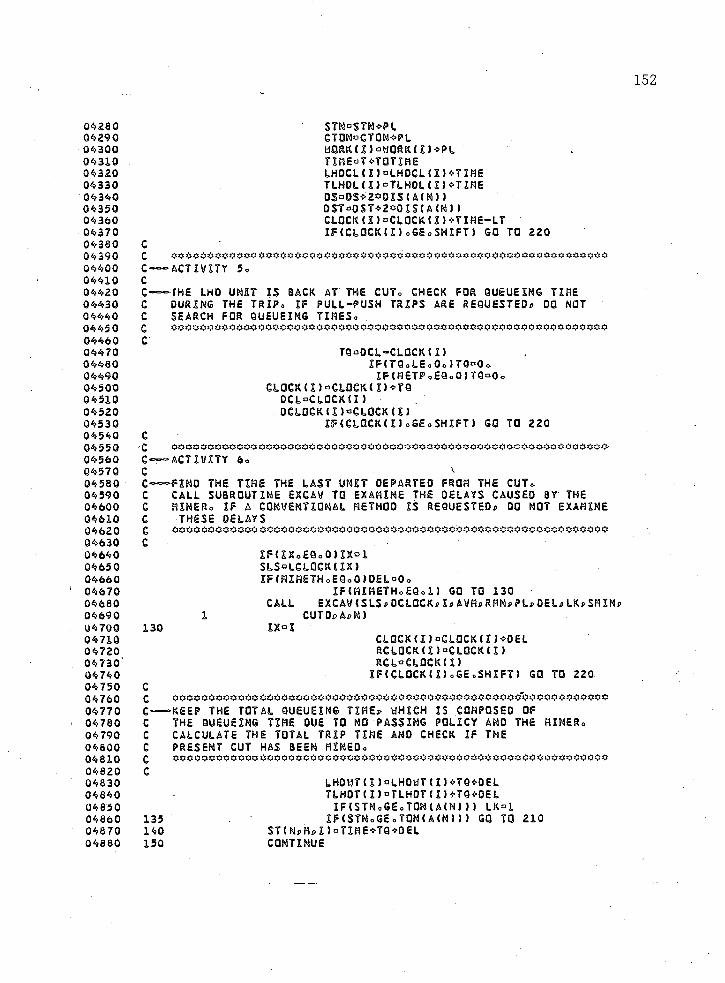
152
0 4 2 8 0 STN=STN*PL0 4 2 9 0 CTONoCTONtPL0 4 3 0 0 WORK C I ) otiORKC I ) *>PL0 4 3 1 0 TINE°T*TQTIHE0 4 3 2 0 LHDCL ( I ) °LH0CL ( I ) <*TIME0 4 3 3 0 TLHDL C I ) °TLH0L C I ) ->TIME0 4 3 4 0 DS °0S» 2» 0XS CA (N ) )0 4 3 5 0 D S T o 0 S T - > 2 » 0 I S C A ( N ) )0 4 3 6 0 CLOCK C I ) oCLOCK C I ) +TIME-LT0 4 3 7 0 IF (CLOCK( I ) o G E o S H I F T ) G O T O 2 2 00 4 3 8 0 C0 4 3 9 0 c 0*****000000ooooOO000000OO000OOOOOOOOOOO0000000000 0000 000*000 4 4 0 0 c ----- ACTIVITY 5 o0 4 4 1 0 c0 4 4 2 0 C------ THE LHO UNIT I S BACK AT THE CUTo CHECK FOR QUEUEING TIME0 4 4 3 0 C DURING THE TRIPo IF PULL-PUSH TRIPS ARE REQUESTED, DO NOT0 4 4 4 0 C SEARCH FOR QUEUEING TIMESo0 4 4 5 0 C **0000000000000000000000000000000000000000000000000000000000-0 4 4 6 0 C0 4 4 7 0 TQoOCL^CLOCKCI)0 4 4 8 0 I F ( T Q o L E o O o ) TQDOo.0 4 4 9 0 IF(METP oEQoO) TQ °0 o0 4 5 0 0 CLOCK(X)°€LQGK( I)*>TQ0 4 5 1 0 DCL° CL OCK (I )0 4 5 2 0 OCLQCK( I ) a CLQCK( I )0 4 5 3 0 I F ( C L Q C K ( I ) o G E o S H I F T ) GO TO 2 2 00 4 5 4 0 C0 4 5 5 0 C oooooooooooooooooooooooooooooooooooooooooooooooooooooooooooo*0 4 5 6 0 C— ‘ ACTIVITY 6o0 4 5 7 0 C V0 4 5 8 0 c ----- >FINO THE TIME THE LAST UNIT DEPARTED FROM THE CUT*0 4 5 9 0 c CALL SUBROUTINE EXCAV TO EXAMINE THE DELAYS CAUSED BY THE0 4 6 0 0 c MINERo IF A CONVENTIONAL METHOD IS REQUESTED, DO NOT EXAMINE0 4 6 1 0 c THESE DELAYS0 4 6 2 0 c ooooooooooooOOOOOOOOOOOOOOOOOOOOOOOOOOOOOOOOOOOOOOOOOO0000000 4 6 3 0 c0 4 6 4 0 I F< I Xo EQ o 0 ) I X ° 10 4 6 5 0 SLS°LCLOCK( IX >0 4 6 6 0 IF(MIHETHoEQoO)DELoOo0 4 6 7 0 I F ( M I M E T H o E Q o l ) GO TO 1 3 00 4 6 8 0 CALL E XC A V( S LS , OC LQC K, I ,AVM ,RMN ,P L, OEL, LK, S MI N0 4 6 9 0 1 C U T D , A , N )0 4 7 0 0 1 3 0 XX°X0 4 7 1 0 CLOCK( I ) °CLQCK( I ) ^ 0 EL0 4 7 2 0 RCLQCK( I ) dCLOCK( I)0 4 7 3 0 RCL°CLQCK( I )0 4 7 4 0 I F ( CLOCK( X)oGE o SH IF T) GO TO 2 2 00 4 7 5 0 c
*******00000 oooooooooooooooooooooooooooooooooooo’booooo 0000000 4 7 6 0 c0 4 7 7 0 CG— KEEP THE TOTAL QUEUEING TIME, WHICH IS COMPOSED OF0 4 7 8 0 C THE QUEUEING TIME DUE TO NO PASSING POLICY AND THE MINER.0 4 7 9 0 c CALCULATE THE TOTAL TRIP TIME AND CHECK IP THE0 4 6 0 0 c PRESENT CUT HAS BEEN MINED.0 4 8 1 0 c0 4 8 2 0 c0 4 8 3 0 LHOWT( X ) °LHOWT( X) ^TQ-frQEL0 4 8 4 0 TLHDT( I ) =TLHDT( I ) fTQ+OE L0 4 8 5 0 IFCSTNoGEoTONCACN)) ) LK°10 4 8 6 0 1 3 5 IF (STNoGE o T Q N ( A ( N ) ) ) GO TO 2 1 00 4 8 7 0 1 4 0 ST( N,M,X>°TXME<‘TQ«‘OEL0 4 6 8 0 1 5 0 CONTINUE
153
04*890 C0 4 9 0 0 C0 4 9 1 0 C----- IF ALL THE LHO UNITS HAVE BEEN FOUND UNAVAILABLE,0 4 9 2 0 C REINITIALIZE THE ARRIVAL TIME IN THE CUT0 4 9 3 0 e oooooooooooooooooooooooooooooooooooooooooooooooooooooooooooo-0 4 9 4 0 C0 4 9 5 0 160 DO 170 IN°1,LNH0 4 9 6 0 IFCLHO <IN 8 oNEo 0 ) GO TO 2 0 00 4 9 7 0 170 CONTINUE0 4 9 8 0 RCLoRCL-t’So.0 4 9 9 0 C05 0 0 0 C oooooooooooooooooooooooooooooooooooooooooooooooooooooooooooo0 50 10 c-----'PLACE THE LHD UNIT AT THE END OF THE QUEUE AND DELETE THE UNIT0 5 0 2 0 c AT THE FRONT05 0 3 0 c 0* 0 * 0 * * 0 0 0 * 0 * 0 0 0 * 0 * * o o o * * * * * O 0 * 0 O O O 0 0 0 0 0 0 0 * 0 0 0 0 * 0 0 O O O * 0 0 0 * 0 00 50 40 c0 5 0 5 0 20 0 CONTINUE0 5 0 6 0 210 CONTINUE0 5 0 7 0 220 CONTINUE0 5 0 8 0 C0 5 0 9 0 C oooooooooooooooooooooooooooooooooooooooooooooooooooooooooooo0 5 1 0 0 C— ='THE SHIFT HAS FIMISHEDoSTOP RECORDING DOWN TIMES0 5 1 1 0 c < S < 1 0 0 0 0 < 1 O < ! $ < > < > <30 5 1 2 0 e0 5 1 3 0 0 0 2 30 1 = 1 , LNH0 5 1 4 0 I F ( C L N ( I ) oNEoOo) GO TO 2300 5 1 5 0 TWN(I)oTWN(I)*SHIFT-CLOCK(I)05 1 6 0 TLtiNCI )oTLtiN<I)«e*SHIFT«CLOCKCI)0 5 1 7 0 230 CONTINUE0 5 1 8 0 c0 5 1 9 0 c * 0 0 0 0 0 0 0 0 0 0 0 0 0 0 0 0 0 0 0 * 0 0 0 0 0 0 0 0 0 0 0 * 0 0 0 0 0 0 0 0 0 0 0 0 0 0 0 0 0 0 0 0 0 0 0 0 0 0 0 -0 5 2 0 0 C----- FORMULATE THE SHIFT RESULTSo0 5 2 1 0 C CALL SUBROUTINES STATIS AND OUTPUT TO ESTABLISH THE STATISTICAL0 5 2 2 0 C PARAMETERS OF THE PRODUCTION DISTRIBUTIONS AND PRINT OUT THE0 52 3 0 C SHIFT RESULTS0 5 2 4 0 c o o o o o o o o o o o o o o o o o o O O O O O O O O O O O O O O O O O O O O * O O O O O O O O O O O O O O O 0 0 0 o o o0 5 2 5 0 c0 5 2 6 0 NS°NS*>10 5 2 7 0 CALL STATISCSTdMNdSO)0 5 2 8 0 00. 260 1= I f LNH0 5 2 9 0 LHOGO olHOCOtLHDGL( I )0 53 0 0 PRT4<I>°TWN(I>0 5 3 1 0 P R C I ) ° ( L H 0 C L ( I ) / S H I F T ) » 1 0 0 o0 5 3 2 0 PRI ( I ) ° t i O R K ( H0 5 3 3 0 IFC PRCDoGT o 100o ) P R ( I ) ° 1 0 0 o0 5 3 4 0 ' 260 CONTINUE0 5 3 5 0 PRT1°ST0N/SHIFT0 5 3 6 0 PRT2°ST0N/LHDCD0 5 3 7 0 P R T 3 °S T 0 N O (D S /3 2 91 ) / SHIFT0 5 3 8 0 WRITEC6f2000)NS0 5 3 9 0 CALL OUTPUT(STONfLHOCOfPRTlfPRT2,PRT3,PRT4,MNfSO,LHDWT,0 5 4 0 0 1 LHOCL,PR,PRI,LNH)0 5 4 1 0 C0 5 4 2 0 C 0000000000000000000000000000000000000000000000000000000000000 5 4 3 0 --- aSAVE THE SHIFT VARIABLES AND CHECK IF MULTIPLE RUNS0 5 4 4 0 C OF THE OPTION I (SEE USER°S GUIDE) ARE REQUESTED,,0 5 4 5 0 C CHECK IP THIS RUN IS THE LAST TO BE PERFORMEDo0 5 4 6 0 C * 0 0 0 0 0 * 0 0 0 0 0 0 * 0 0 0 0 0 0 * 0 0 0 0 0 * 0 0 0 * 0 * 0 0 0 0 0 0 0 0 0 0 0 0 0 0 0 0 * 0 0 0 * 0 0 0 0 0 00 5 4 7 0 c0 5 4 8 0 IF (LStiloEQoQoANOoNSoEQoNOS)GOTO 3800 5 49 0 IFCLSWloEOoOoANDoNSoNEoNOSlGOTO 320

154
0 5 5 0 0 270 SNT CNRUN) °CTON0 55 10 SNAVttCNRUNloAVtt0 5 5 2 0 SNAV( NRUN) d AV0 5 5 3 0 SNGTD( NRUN)oQIS( A( 1 ) )0 5 5 4 0 PT0N°0o0 5 5 5 0 90 280 HXQ°1p IC0 5 5 6 0 PTQN°PTQN->TON <MXQ)0 5 5 7 0 2 8 0 CONTINUE0 5 5 8 0 PTONaPTQN/XC0 5 5 9 0 SN TON( NRUN) °PT0N0 5 6 0 0 GER=Oo0 5 6 1 0 00 300 M0=ljLNH0 5 6 2 0 GERoOER^SPOCHO)0 5 6 3 0 SNLB(NRUN) °SNLB (NRUN )<*0L0A0( I )0 5 6 4 0 SNSP(NRUN) a GER/LNH0 5 6 5 0 300 CONTINUE0 5 6 6 0 C0 5 6 7 0 C 0 0 * * 0 0 * * 0 0 0 0 * * * * * * * * * * * * * * * * * * * * * * * * * * 0 * 0 * * * * * * * * * * 0 * 0 0 * 0 0 * 00 5 6 8 0 C-----•CHECK IF THE MULTIPLE RUMS OF THE OPTION I I (SEE USER'S*GUIDE)0 5 6 9 0 C ARE REQUESTED AND ZERO THE SHIFT VARIABLES FOR THE NEXT RUN0 5 7 0 0 e0 5 7 1 0 c0 5 7 2 0 IF(LSt i loEQoloAN0oLSH2=EQo9 9 oANO.LSU*oEQ.O)RETURN0 5 7 3 0 IF (L SH lo EQolo AN0oLSW2i>EQo996 ANOo LSH^oEQoI) GOTO 3700 5 7 4 0 320 DO 33 0 I ° I p LNH0 5 7 5 0 DCLOCK(I)°Oo0 5 7 6 0 LCLOCK(l)°Oo0 5 7 7 0 LHOUTCDoOo05 780 LHDCL(I )°0=0 5 7 9 0 CLOCK( I ) D0o0 5 8 0 0 CLN (I ) °Oo0 5 8 1 0 HORKtI) °0o0 5 8 2 0 330 T t i N ( I ) ° 0 »0 5 8 3 0 DS°Oo0 58 4 0 LHOCO°Oo0 5 8 5 0 STONoOo0 5 8 6 0 SL S=0 »0 5 8 7 0 OCL °0o0 5 8 8 0 RCL°Oo.0 5 8 9 00 5 9 0 0 IF( LSHlo£QoloANDoLSti2oNE<i99) NS=00 5 9 1 0 RCLOCK( 1 ) °1<>0 5 9 2 0 IFCLNHqEQoI ) GO TO 3300 5 9 3 0 0 0 3 4 0 I.°lfl LI0 5 9 4 0 340 RCLOCK(H-l )°RCLOCK(I)<- lo0 5 9 5 0 350 CONTINUE0 5 9 6 0 IFTLStiloEQo 1 oAND<iLSU2oNE<i99)RETURN0 5 9 7 0 IF(L SU loE QoO ) GO TO 1330 5 9 8 0 C0 5 9 9 0 c0 6 0 0 0 C----- GALL SUBROUTINE PLTXNT TO INITIALIZE THE ARRAY TO BE PLOTTEOo0 6 0 1 0 C FORMULATE AND PRINT THE FINAL RESULTS.0 6 0 2 0 c0 6 0 3 0 C0 6 0 4 0 370 CALL PLTINT(NES»SNT»SNLB»SNAV»SNAVM#SNCTD»SNSP»SNTON»0 6 0 5 0 1 NRUNjjLPR)0 60 6 0 RETURN0 6 0 7 0 380' tiRITE (6p 2 0 1 0 ) ZNAME1# ZNAME2j>OATE1»DATE2»NOS06 0 8 0 00 410 I D1» LNH0 6 0 9 0 TLHOC°TLHDC<-TLHOL(I)0 6 1 0 0 P R T 4 ( I ) ” TLt iN( I )

155-
0 6 1 1 0 PR( I ) = < TL HOL( I ) / ( N0S4SHIFT) ) a 100 o06 1 2 0 PR1( I ) QtfGRK( I )0 6 1 3 0 XF( PR( D o G T o l Q O o ) P R < I ) ° 1 0 0 o0 6 1 4 0 410 CONTINUE0 6 1 5 0 PRT1°CT0N/(NOSaSHXFT)0 6 1 6 0 PRT2°CTQN/TLH0C0 6 1 7 0 • PRT3DCTQNa<0S(f 3 2 8 1 ) / SHIFT0 6 1 8 0 CALL STATIS(ST,MMpSD)0 6 1 9 0 CALL OUTPUT ( CTONp TLHOCp PRTl^ PRT2j? PRT3p PRT4» MNp SOp TLHOT0 6 2 0 0 1 TLHDLpPR,PRljLNH)0 6 2 1 0 420 RETURN0 6 2 2 0 2000 FORHAT( I H l p 2 0 X p l S H I F T " , 2 X , X 2 / / )0 6 2 3 0 2010 F0RMAT(/ /1H1 j>20X/> eS I M U L A T I O N R E P O R T V / /0 6 2 4 0 1 20X^2A8j)4Xj,2A8/20Xp c UNIVERSITY OF ARIZONA COLLEGE OF MINES'06 25 0 2 20Xp 'TOTAL NUMBER OF SHIFTS SIMULATED*,2X,1 2 / / )0 6 2 6 0 END0 6 2 7 0 SUBROUTINE AVAIL( AV,LHOd I )0 6 2 8 0 C o o o o a a a o o o o a * o o a o o o o o a o o o a < i o o o < : a a * * o a a a a a o a a o a o o o a a a o o o o o a a o0 6 2 9 00 6 3 0 0 c----- THIS SUBROUTINE CHECKS. THE AVAILABILITY OF THE CALLED UNIT06 3 1 00 6 3 2 0 c0 6 3 3 00 6 3 4 0 DIMENSION LH0C10)0 6 3 5 0 c0 6 3 6 0 c o o o o a a a a o o a o o a o a a a o o o a o o o a o a a o o o a o a o a o a o a a a o o o o a a o a o o o a o o o o *0 6 3 7 0 c -- CALL A RANDOM NUMBER0 6 3 8 0 c0 6 3 9 0 c0 6 4 0 0 RN°RANF<0 o )0 6 4 1 0 c0 6 4 2 0 c0 6 4 3 0 C-9— IF THE CALLED RUNOOH NUMBER IS GREATER THAN THE0 6 4 4 0 c AVAILABILITYf THEN THE LHO UNIT IS NOT AVAILABLE0 6 4 5 0 c O O O O l X l <■<!<!<1<1<1<1<1 <1<1<I<1<S<!<i< 5 < 1 0 1 ) < ■ < ! < >0 6 4 6 0 c0 6 4 7 0 I F( RNo GE oAV) GO TO 100 6 4 8 0 c0 6 4 9 0 c 0 0 0 0 0 0 0 0 0 0 0 0 0 0 0 0 0 0 0 0 0 0 0 0 0 0 0 0 0 0 0 0 0 0 0 0 0 0 0 0 0 0 0 0 0 0 0 0 0 0 0 0 0 0 0 0 0 0 0 00 6 5 0 0 c — •THE CALLED RANDOM NUMBER IS SMALLER THAN THE AVAILABILITY,06 5 1 0 c THE LHO UNIT IS AVAILABLE0 6 5 2 0 c 0 0 0 0 0 0 0 0 0 0 0 0 0 0 0 0 0 0 0 0 0 0 0 0 0 0 0 0 0 0 0 0 0 0 0 0 0 0 0 0 0 0 0 0 0 0 0 0 0 0 0 0 0 0 0 0 0 0 0 *0 6 5 3 0 c0 6 5 4 0 LHD(I ) ° 10 6 5 5 0 GO TO 200 6 5 6 0 10 LHO(X ) n00 6 57 0 20 CONTINUE0 6 5 8 0 RETURN0 6 5 9 0 END0 6 6 0 0 "0 6 6 1 0 SUBROUTINE NORMCM , S , X , N)06 6 2 0 c 00* 00000*000 O O O O O O O O O O O O O O O O O O O O O O O 00* 00o o o o o o o o o o o o o o o o o o o o0 66 300 6 6 4 0 c--- THIS SUBROUTINE GENERATES RANDOM VALUES FOLLOWING0 66 5 0 c THE NORMAL DISTRIBUTION0 6 6 6 00 6 6 7 0 c o o o o o o 0 0 0 0 0 0 0 * 0 0 0 0 0 0 0 0 0 0 0 0 0 0 0 0 0 0 0 0 0 0 0 0 0 0 0 0 * 0 O O O O O O O O O O O O O 0 0 006 6 8 00 6 6 9 0 REAL M0 6 7 0 0 DIMENSION M ( I 0 ) , P ( 7 ) i > S ( 1 0 ) , Z C 7 )06 71 0 OAT A Z / = 3 o , —2 o » “ l o p Oop l o p 2op 3o /

156
0 6 7 2 0 DATA P Z 0 o j> Oo05» Ool6p OoS# OoS5# 0o95j>. l o /0 6 7 3 0 RN°RANF<0o)0 6 7 4 0 DO 10 I ° l » 606 7 5 0 IF( < R N o 6 £ o P m ) < , A N 0 o ( R N o l E o P < m ) ) > GO TO 200 6 7 6 0 10 CONTINUE06 770 20 Z N ° (Z C I» l)< -< R N H > m ) » Z ( I ) o ( P < H - l ) ~ R N n / ( P ( I * l ) - P ( X ) )0 6 7 8 0 XoM(N)+S(N)*ZN0 6 7 9 0 RETURN0 6 8 0 0 END0 68 100 6 8 2 0 SUBROUTINE TOTCYC ( I j>TOTIREi> LT»OT»OISi>ACR» BRR» 6»N» UU L0» SHAUU0 6 8 3 0 1 SCUT„SOUMP)0 6 6 4 0 ,
0 6 8 5 0 C0 6 8 6 00 6 8 7 0 c ™ •THIS SUBROUTINE CALCULATES THE ONE-WAY TRIP OF A LHO UNIT0 6 8 8 0 c INCLUDING THE LOADING AND DUMPING TIMES.0 6 8 9 006 9 0 0 c 0 0 0 0 0 0 0 0 0 0 0 0 0 0 0 0 0 0 0 0 0 0 0 0 0 0 6 0 0 0 6 6 0 0 0 0 0 0 0 0 6 6 0 0 0 0 0 0 0 0 0 6 0 0 0 0 0 0 0 00 6 9 1 00 6 9 2 0 REAL L0» LLdLT0 6 9 3 0 DIMENSION A ( 6 0 ) » 0 I S ( 6 0 ) » LD( 6 0 ) # LLC 6 0 )06 9 4 0 DIMENSION PIL (1 0 ) t SDK 1 0 )0 6 9 5 0 c0 6 9 6 0 c o o o o o o o o o o o o 0 0 0 0 0 0 0 0 0 0 0 0 0 0 0 0 0 0 0 0 0 0 0 0 0 0 0 0 0 0 * 0 0 0 0 0 0 0 0 0 0 0 0 0 0 0 0 00 69 70 C----- CALL SUBROUTINE NORM TO CALCULATE THE DUMPING TIME*0 6 9 8 0 C THE LOAD TIME HAS ALLREADY BEEN CALCULATED IN THE MAIN PROGRAM0 6 9 9 0 C 0 0 0 0 0 0 0 0 0 6 0 0 0 0 0 0 0 0 0 0 0 * 0 0 * 0 0 0 0 * 0 0 * * 0 0 0 0 0 0 0 0 0 0 0 0 0 0 0 0 0 0 0 * * 0 0 * 0 00 7 0 0 0 C0 7 0 1 0 CALL NOR M(PILfSDl fOTfI )0 7 0 2 0 c07030*' c O O O O O O O O O O O O 0 0 0 0 0 0 0 0 0 0 0 0 0 0 0 0 0 0 0 0 0 0 0 0 0 0 0 0 0 0 0 0 0 0 0 0 0 0 0 0 0 * 0 0 0 0 0 00 7 0 4 0 c -----•CALL SUBROUTINE CYCLE TO ESTABLISH THE TRIP TIME0 7 0 5 0 c WITHOUT THE DUMPING AND LOADING TIME0 7 0 6 0 c 0 0 0 0 0 0 0 0 0 0 0 0 0 6 0 0 0 0 0 0 0 0 0 0 0 0 0 0 0 0 0 0 0 0 0 0 0 0 *0 0 0 0 0 0 0 0 0 0 0 0 0 0 0 0 0 0 0 0 00 7 0 7 0 c0 7 0 8 0 CALL CYCLE (DI5» ACRp BRRp AjjTp Np LLj>LO»SHAUL»SCUTj>SDUMP )0 70 90 c0 7 1 0 0 c 0 0 0 0 0 0 0 0 6 0 6 0 0 0 0 0 0 0 6 0 0 0 0 0 0 6 0 0 0 0 0 0 0 0 0 0 6 0 0 0 0 0 0 0 0 0 0 0 0 0 0 0 0 0 0 0 0 0 0 0
0 7 1 1 0 c~=~•CALCULATE THE TOTAL ONE WAY TRIP TIME INCLUDING THE LOADING0 7 1 2 0 c AND DUMPING TIME07 1 3 0 c ##*#00000000#######0000000oooooooooooooooooooooooooooooooooo0 7 1 4 0 c0 7 1 5 0 TOTIME°LT*DT*T0 7 1 6 00 7 1 7 0 RETURN0 7 1 8 0 END0 7 1 9 00 7 2 0 0 SUBROUTINE CYCLE ( OIS» ACR» 8RRi> A»Ti>NpLL»LD»SHAUL»SCUT#SDUMP )0 7 2 1 0 c O O O O O O O O O O O O 0 0 0 0 0 0 0 0 0 0 0 0 6 0 0 0 0 0 0 0 0 0 0 0 0 0 0 0 0 0 0 0 0 0 0 0 0 0 0 0 0 0 0 0 0 0 0 0
0 7 2 2 00 7 2 3 0 c — •THIS SUBROUTINE CALCULATES THE TRAVEL TIME FROM THE DUMP TO0 7 2 4 0 c THE OPERATING CUT0 7 2 5 00 7 2 6 0 c0 7 2 7 0 REAL LOp LL07 28 0 DIMENSION A ( 6 D ) j i 0 I S ( 6 0 ) » L 0 ( 6 0 ) i > L L ( 6 0 )0729 0 c0 7 3 0 0 c oooooooooooo0 0 0 0 0 0 0 O O O O O O O O O O O O **********0 0 0 OOOOOOOOOOOO*0000 7 3 1 0 c — •CALCULATE THE TIME NEEDED BY THE LHO UNIT TO COVER0 7 3 2 0 c THE DUMP CHANGE-OUT DISTANCE.
157
07 33 0 C FIND THE ACCELERATION TIME AND DISTANCE, THE DISTANCE0 7 3 4 0 C LEFT TO BE COVERED BY CONSTANT SPEED AND FINALLY,0 7 3 5 0 c THE TOTAL TIME07 3 6 0 c0 7 3 7 0 I F ( I D ( A ( N ) ) oEOoOo) GO TO 100 7 3 8 0 ACT °SDUMP/ACR0 7 3 9 0 AC0 = ( l « / 2 o )»ACR<=(ACT*»2)0 7 4 0 0 . ACONO°LO( A(N ) ) —ACO0 7 4 1 0 ACONToACOND/SDUMP07 4 2 0 TIM1°ACT*AC0NT0 7 4 3 0 GO TO 200 7 4 4 0 10 TIHl=Oo0 7 4 5 0 c0 7 4 6 0 c0 74 7 0 c—-CALCULATE THE TIME NEEDED TO COVER. THE HAUL DISTANCEo0 7 4 8 0 c FIND THE BRAKING TIME AND DISTANCE, THE DISTANCE LEFT TO0 7 4 9 0 c BE COVERED BY CONSTANT SPEED AND FINALLY, THE TOTAL HAUL TIME0 7 5 0 0 c O O O O O O 0 0 0 0 0 0 0 0 0 0 0 0 O O O O O O O O O O O O 0 0 O O O O O O O O O O O O O O O O 0 0 * 0 0 0 0 0 0 0 0 00 7 5 1 0 c07 5 2 0 20 ACT oCSHAULMSDUMP) / ACR0 7 5 3 0 ACO o( lo /2 o ) *A CR * (A C T 0 02 )0 7 5 4 0 BRT° (SHAU L"SCUT) / 8RR0 7 5 5 0 B R D ° < l c / 2 c ) 0 8 R R o ( B R T o * 2 )0 7 5 6 0 ACONO°OIS ( A( N) ) —LL ( A (N ) ) - L D (A (N ) )«»8R0»ACD.0 7 5 7 0 ACONT °ACONO/SHAUL0 7 5 8 0 Tlf l 2 = ACT*BR'T*AC0NT0 75 90 c0 76 0 0 c 0 0 o o o o o o o o o o 0 0 0 0 * 0 0 0 0 * 0 0 0 0 0 0 0 0 0 0 O O O O O O O O O O O O O O O O O O O O O O O O O O O O0 7 6 1 0 c—"CALCULATE THE TIME NEEDED TO COVER THE CUT CHANGE-OUT DISTANCE0762 0 c FIND THE BRAKING TIME AND DISTANCE,THE DISTANCE0 7 6 3 0 c LEFT TO BE COVERED WITH CONSTANT SPEED AND FINALLY , THE TOTAL0 7 6 4 0 c 0 * 0 0 * 0 O O O O O O 0 0 0 0 0 0 * 0 * 0 0 0 0 0 * 0 0 0 0 0 0 * 0 0 0 * 0 0 0 0 * 0 0 0 * 0 O O O O O O 0 * 0 0 0 00 7 6 5 0 c0 7 6 6 00 7 6 7 0 IF (L L (A (M )) o E Q o 0o ) GO TO 3007 6 8 0 BRT °SCUT/BRR0 7 6 9 0 B R 0 ° ( l o / 2 o )<'BRR<1(BRT0<'2)0 7 7 0 0 6C0N0nt.L (A (M) )=BRO0 7 7 1 0 ACOMToACONO/SCUT0 7 7 2 0 TIM3 ° ACONT*BRT0 7 7 3 0 GO TO 400 7 7 4 0 30 TIM3°0o07 75 0 c0 77 60 c O O O t S O O O O O i S O O O O O O O O O O O O O O O ' X i O O i S O O i S O O 0<1O6<I<3<I <1O 6O<1<1<1O <10 77 70 c ~ -CALCULATE THE TOTAL TRIP TIME0 7 7 8 0 c 000000000000 # * * 00* * * 00000# 0 0 0 0 0 0 0 0 0 0 0 0 0 0 0 0 0 0 0 * 0 0 0 0 * 0 * * 0 * 0 0 0 00 7 7 9 0 c0 7 8 0 0 40 T^TIMH-TIMZ^TIMB0 7 8 1 0 RETURN0 78 2 0 END0 7 8 3 007 8 4 00 7 8 5 0 SUBROUTINE STATIS(X,MN,SD)u 78 60 c 000000O O O O O O 00000000000000000000000O O O O O O 0 0 0 O O O O O O 00000000 0 00 7 8 7 00 7 8 8 0 c—-TH IS SUBROUTINE FINDS THE MEAN AND THE STANDARD DEVIATION OF A0 78 9 0 c STATISTICAL POPULATION0 7 9 0 00 7 9 1 0 c O O O O O O O O O O O O o o o o o o o o o o # * * * 00000 0 # 0 0 0 0 0 0 0 0 0 * 0 0 0 0 0 0 * 0 0 0 0 0 0 0 0 0 00 79 200 7 9 3 0 REAL MN

158
07 9 4 0 DIMENSION X( 6 Op 3 Op 10 )0 7 9 5 0 C0 79 60 C 0 * 0 0 0 0 0 0 6 0 * 0 0 0 0 0 0 0 0 0 0 0 0 0 0 0 0 0 0 0 0 0 0 0 0 0 0 0 0 0 0 0 0 0 0 0 0 0 0 0 * 0 0 0 0 0 0 0 0 0U7970 C ™ FIND THE MEAN0 7 9 8 0 c * * * * * * * * * * * * * * * * * * * * * * * * * * * * * * * * * * * * * * * * * * * * * * * * * * * * * * * * * * * *0 79 9 0 c0 8 0 0 0 S=0o0 8 0 1 0 K=00 8 0 2 0 00 10 N=1j>600 80 30 00 10 f l o l # 300 80 40 00 10 111,100 8 0 5 0 I F (X (N » M , I )o E Q o O o ) GO TO 100 8 0 6 0 S ° S * X ( N , M , I )0 8 0 7 0 K.eK+10 80 80 10 CONTINUE0 8 0 9 0 MW=S/K0 8 1 0 0 c0 8 1 1 0 c * * * * * * * * * * * * * * * * * * * * * * * * * * * * * * * * * * * * * * * * * * * * * * * * * * * * * * * * * * * *0 8 1 2 0 c----- FIND THE STANDARD DEVIATION0 8 1 3 0 c0 8 1 4 0 c0 8 1 5 0 S° 0o0 8 1 6 0 00 20 N ° l , 600 8 1 7 0 00 20 R ° l , 300 8 1 8 0 00 20 1 = 1 , 1 00 8 1 9 00 8 2 0 0
• I F ( X ( N , N , I ) o E Q o O o ) GO TO 20Y ° X (N , H , I 1 - f l N
0 8 2 1 0 SY=Y<i»20 8 2 2 0 S°S->SY08 230 20 CONTINUE0 8 2 4 0 SO°SQRTIS/ ( K - l ) )0 8 2 5 0 RETURN0 8 2 6 0 END08 2 7 00 8 2 8 0 SUBROUTINE OUTPUT( STON,LH0C0,PRT1,PRT2,PRT3,PRT4»MN,SO,LHOWT,0 8 2 9 0 1 LHOCL,PR,PR1,LNH)0 8 3 0 0 c * * * * * * * * * * * * * * * * * * * * * * * * * * * * * * * * * * * * * * * * * * * * * * * * * * * * * * * * * * * *0 8 3 1 00 83 2 0 ' 08 3 3 0
THIS SUBROUTINE PRINTS OUT THE SIMULATION REPORT
0 8 3 4 0 e0 8 3 50 REAL LHOCL,LHOCO,LHOtiT,HN0 83 60 DIMENSION L H 0 C L ( 1 0 ) , L H 0 W T ( 1 0 ) , P R ( 1 0 ) , P R T 4 < 1 0 ) , P R 1 ( 1 0 )08 3 7 0 c0 83 80 c08 390 c--- •PRINT OUT THE PRODUCTION SUMMARY0 8 4 0 0 e <1 <1 <1 <1 <lO<1 <1 t"tl <10<1 <!<t<l<1 <1 <10<1 tl=><1<1 <S1S<1<1<1 W O * * ’)0<I<!0 8 4 1 0 e0 8 4 2 0 tiRITE( 6 , 2 0 0 0 )0 8 4 3 0 WRITE( 6 , 2 0 1 0 )STON,LHOCO,PRT1,PRT20 84 4 0 c0 8 4 5 0 c <1<S<1<1<1<1<1<1<1<I<1<1<1<I<1<S<1<I<1<1<1<I<1<1<1<1<1<I<1<1<1<I<1<1<1<1<1<1<1<1<I<1<1<1<1<1<S<1<1<1<1<1<1<S<1<I<1<I<1<1
08 4 6 0 c— ■PRINT OUT THE HAULAGE SUMMARY0 84 70 c OOOiSCi <1<I<1<1<S <I<1<1<1<1 <1<5<1<1<1 <1<1<1<11S <1<1<1<1<1 <1<1<1<1<1 "SOWS <1<1<1<1<1 <1<1<1<1<1 <1<1<1<1<1 <1<1<1<1<1
0 8 4 8 0 c0 8 4 9 0 t iRITE(6p2 020 >0 8 5 0 0 t iRITE(6p 2 0 3 0 JMNp SDp PRTS0 8 5 1 0 c0 8 5 2 0 c * * * * * * * * * * * * * * * * * * * * * * * * * * * * * * * * * * * * * * * * * * * * * * * * * * * * * * * * * * * *0 8 5 3 0 C — PRINT OUT THE WAIT TIME ANALYSIS0 8 5 4 0 C * * * * * * * * * * * * * * * * * * * * * * * * * * * * * * * * * * * * * * * * * * * * * * * * * * * * * * * * * * * *

159
0 8 5 5 0 C0 8 5 6 0 tiftXTE < 6x>2 0 4 0 )0 8 5 7 0 DO 10 I ° 1 j?LNH0 8 5 8 0 tiRI 7E ( 6p 2 0 5 0 ) Ij) LHOCL< X) p LHOtiT C K ) j > P R T 4 ( l ) p P f t ( I ) p P R l ( I )08 590 10 CONTINUE0 8 6 0 0 RETURN0 8 6 1 0 2000 FORMAT.(1Xp 20X p 1P R O O U C T I O N S U M M A R Y * / / >0 8 6 2 0 2010 FQRMAKIOXp °TONS DELIVERED TO THE DUMPS0 8 6 3 0 1 IXp T60pF9 o 3 / /0 8 6 4 0 2XXp 9Xp 1 MACHINE MINUTES SIMULATED*,0 8 6 5 0 3 IXp T60 p F9 o 3 / /0 8 6 6 0 4 1X»9Xj> •PRODUCTION RATE IN TONS PER MINUTES0 86 7 0 5 1Xp T 6 0 p F 9 o3 / /0 8 6 8 0 6 1Xp 9Xp •PRODUCTION RATE IN TONS PER MACHINE MINUTES0 8 6 9 0 7 IXp T60 p F9o 3 / / / )08 7 0 0 2020 FQRMAK1 Xp 20Xp °H A U L A G E S U M M A R Y S / )0 8 7 1 0 2030 FORMATdOXp • AVERAGE LHO CYCl£ S IX p T 60 , F9 o3 / /0 8 7 2 0 r 1 lOXp ^STANDARD DEVIATIONS 1 Xp T 6 0 p F9o3 /Z0 8 7 3 0 2 IXp 9Xp ” PRODUCTION RATE IN KILOMETER TONS/MINS0 8 7 4 0 3 1Xp T 6 0 p F 9 o3 / / / )0 8 7 5 0 2040 FORMAT d X p 2 0 X p °ti- A I T T I M E A N A L Y S I S ° / / )0 8 7 6 0 2050 FQRMATdXp4Xp 8 LHO UNIT S 2Xp • WORKING T IM E S Z X p0 8 7 7 0 1 0WAITING. TIME S 2 X p flDOtiN TIME S2 Xp° UTILIZATION PRC S 2 X p0 8 7 8 0 1 °LQAD HAULED 0 $ /0 8 7 9 0 2 8Xp 12 , 5 X , F 9 o3 p 5 X , F 9 o,3p 5Xp F 9 o3 p 5Xp F 9 o3 p 5 X , F 9 o3)0 88 00 END0 8 8 1 00 8 8 2 00 8 8 3 0 SUBROUTINE EXCAV( SLSp OCLOCK,I,AVMpRMN,PL,DEL,LKp SMINp CUTD,Ap N)0 88 40 C0 8 8 5 00 8 8 6 0 C----- THIS SUBROUTINE EXAMINES THE ACTIVITY OP EXCAVATION AND0 8 8 7 0 C REPORTS POSSIBLE DELAYS CAUSED BY THE MINER0 8 8 8 00 8 8 9 0 C O O O O O O O O O O O O O W O O O O O O O O O O O O O O O i M O O O O O O O O O i M i O O O z M O O O O O O O O i M O #
0 8 9 0 00 89 10 DIMENSION A ( 3 Q ) » € U T 0 ( 3 Q ) »OCLOCK( 1 0 )0 8 9 2 0 c0 8 9 3 0 c < I< 1< 1< 11S < 1 < 1 < 1 < 1 < 1 < 1 < 1 < 1 < 1 < 1 < 1 < 1 < 1 < 1 < 1 < 1 < 1 < 1 < 1 < 1 < 1 < 1 < 1 < 1 < 1 < 1 < 1 < 1 < 1 < 1 < 1 < 1 < 1 < 1 < 1 < 1 < 1 < 1 < 1 < 1 < 1 < 1 < 1 < 1 < 1 < 1 < 1 < 1 < 1
0 8 9 4 0 CHECK IF THE MINER HAS TO MOVE TO THE NEXT CUT. IF IT HAS TO MOVE,08 9 5 0 c FIND THE TIME IT HILL BE READY TO LOAD THE JUST ARRIVED UNIT0 8 9 6 0 c ( i < : < i < i < 1<1< 1< 1< 1 < H S < 1 < 1 < 1 < 1 < 1< 1< 1< 1< 1 < 1<1< 1< 1< 1 < 1 < 1< 1< 1< 1 < 1<1< 1<1< 1 < 1<1< 1< 1< 1 < 1<1< 1<1< 1 < !< ; < ! < 1<1< 1< 1< 1 < 1< 1< 1< 1< 1< 1< 1
0 8 9 7 0 c0 8 9 8 0 IFtLKoEQoO) GO TO 100 8 9 9 0 TM°CUTD(A(N) )/SMIN0 9 0 0 0 SL=SLS*TM0 9 0 1 0 . GO TO 200 9 0 2 0 c09 0 3 0 c < l< t < 1< 1 < 1< 1< 1<1 < 1 < 1< 1< 1< 1 < 1< 1< 1< 1< I < I < 1 < I < I <1 < I < 1< 1 < 1< 1< I < 1 < I < 1 < 1 < 1<1 < 1 < 1< 1< 1< 1 0 < 1 <1 <1 < 1 <1< I <1 < 1< 1 < I <1 < 1< I < I < 1< 1 < 1< 1<1
0 9 0 4 0 c ------ COMPUTE THE TIME BETWEEN AN ARRIVAL OF AN LHD AND THE0 90 5 0 c TIME THE MINER IS READY TO START LOADING09 0 6 0 c0 9 0 7 0 c0 9 0 8 0 10 SL° SLS0 9 0 9 0 20 TPR°OCLOCK(I)e SL0 9 1 0 0 IF(TPR) 3 0 , 4 0 , 400 9 1 1 0 30 CONTINUE09 1 2 0 C09 1 3 0 C 0 0 0 0 0 0 0 *0 0 0 0 0 0 0 0 0 0 0 0 0 0 0 0 0 0 0 0 0 0 0 0 0 0 0 0 0 0 0 0 *0 0 0 0 0 0 0 0 0 0 0 0 0 0 0 0 0 0 00 9 1 4 0 Cr— •THE LHO IS READY FOR LOADING HHEN ITS PREDECESSOR IS09 15 0 C STILL GETTING LOADED.

160
0 9 1 6 0 C KEEP THE WAITING TIME TILL THE MINER IS FREE AND CALCULATE0 9 1 7 0 C THE AVAILABLE ORE AT THE FACE AFTER THE DEPARTURE OF THE0 9 1 8 0 C PRECEEDING UNIT0 9 1 9 0 C0 9 2 0 0 c0 9 2 1 0 S 0 oe=TPR0 9 2 2 0 TORE°REM0 9 2 3 0 GO TO 5 00 9 2 4 0 4 0 CONTINUE0 9 2 5 0 C0 9 2 6 0 0 * 0 * 0 0 0 0 0 0 0 0 0 0 0 0 0 0 * 0 * 0 0 0 0 0 0 0 0 0 0 0 0 0 0 0 $ * GOO0 9 2 7 0 THE LHD I S READY FOR LOADING WHEN THE MINER IS FREEo0 9 2 8 0 C COMPUTE THE ORE EXTRACTED BY THE MINER WHEN IT WAS FREE ANDU 9 2 9 0 c UPDATE THE ORE STOCK AT THE FACE0 9 3 0 0 o o o o o o o o o o o o OOOO0 0 0 0 0 0 0 * 0 0 0 0 0 0 0 0 0 0 0 0 0 0 0 0 0 0 0 0 0 0 0 0 0 0 0 OOO GOO0 0 00 9 3 1 0 c09 3 2 0 TPRM°TPR*AVN0 9 3 3 0 ORE°TPRMORMN0 9 3 4 0 TORE=ORE+.REM0 9 3 5 0 I F ( TQ REo LTo P L) GO TO 450 9 3 6 0 c0 9 3 7 0 c * * * * * * 0 0 * * 0 * * * * * * * * 0 0 0 * 0 0 0 0 0 * 0 0 0 0 0 0 OOOO0 0 OOOOOOOOOOOOOOO*OOO0 9 3 8 0 c---------- SINCE THERE IS ENOUPH ORE STOCK AT THE FACE,0 9 3 9 0 c THE LHD CAN GET LOADED AT ONCE0 9 4 0 0 c * 0 * * * 0 0 0 0 * * * 0 * 0 0 0 0 0 0 0 0 0 0 0 0 0 0 0 0 0 0 0 0 0 0 0 0 0 0 0 0 0 0 0 0 0 0 0 0 0 0 0 0 0 0 0 0 0 00 9 4 1 0 DEL ° 0 o0 9 4 2 0 REM °TOREe PL0 9 4 3 0 GO TO 6 00 9 4 4 0 45 S 0 ° 0 o0 9 4 5 0 «c0 9 4 6 0 c * * * * * 0 * * * * 0 * * 0 0 * 0 * * 0 * * 0 * 0 * 0 0 * 0 * 0 0 0 * * 0 0 0 0 0 0 0 0 0 0 0 0 0 0 0 0 0 0 0 0 0 0 0 00 9 4 7 0 c----------'THE LHD MAY HAVE TO tiA£T FOR THE MINER TO EXCAVATE ENOUPH ORE0 9 4 8 0 c CALCULATE THE ORE QUANTITY THE "MINER HAS TO EXCAVATE0 9 4 9 0 .c AND UPDATE THE REMAINING STOCK AT THE FACE0 9 5 0 0 c0 9 5 1 0 c0 9 5 2 0 5 0 DMN=PL-TORE0 9 5 3 0 REM°Oo0 9 5 4 0 IF(DMNoLT o O o ) REMoTQRE^PL0 9 5 5 0 IFCDMNoLToQo)OMN*Oo0 9 5 6 00 9 5 7 0 C 0 * 0 0 0 0 0 0 0 0 0 0 0 0 0 0 0 0 0 0 0 0 0 0 0 0 0 0 0 0 0 0 0 0 0 0 * * * 0 0 0 0 0 * 0 0 0 0 0 * 0 0 0 0 0 0 0 * 00 9 5 8 0 c--- •CALCULATE THE TOTAL DELAY DUE TO THE MINER. THIS DELAY0 9 5 9 0 c CONSISTS OF THE TIME THE LHD HAS TO WAIT FOR THE MINER TO BE0 9 6 0 0 c AND THE TIME OF THE EXCAVATION ACTIVITY0 9 6 1 0 c0 9 6 2 0 c0 9 6 3 0 HER°OMN/RNN0 9 6 4 0 DEL=<tiER/AVM)<-SQ0 9 6 5 00 9 6 6 0 6 0 CONTINUE0 9 6 7 0 LK = 00 9 6 8 0 RETURN0 9 6 9 0 END0 9 7 0 009 7 1 009 7 2 0 SUBROUTINE H IS T O( S MT , SE M ,N E S, L PR , NR U N)0 9 7 3 00 9 7 4 0 G < ! < 1 < ! <1 <! <1 POQ <1 < !< ! < !< 1 < ■ < !I ) I ? ■><! <! <!
0 9 7 5 00 9 7 6 0 C — •THIS SUBROUTINE PLOTTES HISTOGRAMS IN THE LINE PRINTER

09 7 7 00 9 7 8 0 C0 9 7 9 0 DIMENSION MARKS( 1 0 ) , SEN( 1 0 ) , SNT( 1 0 )0 9 8 0 0 DATA I AST / IHO/0 9 8 1 0 C0 9 8 2 0 C 0 0 * 0 0 * 0 0 * 0 * 0 0 0 0 0 0 0 0 0 0 0 0 0 0 0 0 0 0 0 0 0 0 0 0 0 0 0 0 0 0 0 0 0 0 0 0 9 0 0 * 0 0 0 * 0 0 0 0 00 9 8 3 0 C----- •RECORD THE RESULTING PRODUCTION WITH A 1*25 SCALE0 9 8 4 0 c 0 0 * 0 0 0 OOOOOO OOOOOoOOO0 * 0 0 0 0 0 0 0 0 0 0 * 0 0 0 0 * * 0 0 * 0 0 0 * 0 0 * 0 0 0 0 * 0 0 0 0 00 9 8 5 0 c0 9 8 6 0 DO 30 Iolj)NRUN0 9 8 7 0 DO 10 j o l f 500 9 8 8 0 IF(SNT ( I ) . l E o u<" 25 . ) o A N O .S N T m o G T , U - 1 ) 0 Z S < , I GO TO 200 9 89 0 10 CONTINUE0 9 9 0 0 20 HARKS ( I ) ° J0 9 9 1 0 30 CONTINUE0 9 9 2 0 IF(NE SoE Qo l ) GO TO 400 9 9 3 0 I F ( N E S o E 9 o 2 ) GO TO 500 9 9 4 0 I F ( N E S o E 0 o 3 ) GO TO 600 99 5 0 IF(NESoEQo4) GO TO 7009 9 6 0 IF (N E So E9 o5) GO TO 8009 9 7 0 IF(NES<,E9o6) GO TO 900 9 9 8 0 C0 9 9 9 0 C10 00 0 C----- PRINT THE TITLE OF THE HISTOGRAM .1001 0 C 3 3 3 3 3 0 3 3 3 3 3 3 3 3 3 3 3 3 3 0 3 3 3 3 3 3 3 3 3 3 3 3 3 3 0 3 3 3 3 3 3 3 3 3 3 3 3 3 3 3 3 3 3 0 3 3 3 3 3 31002 0 C10 03 0 40 ZNAHlnlOHLHO AVAILA100 4 0 ZNAH2°10HBILITY10 050 GO TO 1 0 0100 60 50 ZNAH1°10HMINER AVAI10 0 7 0 ZNAH2=10HLABILITY1 00 80 GO TO 1 0 010 090 60 ZNAH1=10HCUT-0UHP1 01 00 ZNAH2°10HDISTANCE1 0 1 1 0 GO TO 10010 12 0 70 ZNAH1olOHAVERAGE1 013 0 ZNAH2°10HLH0 SPEED10 14 0 GO TO 10010 1 5 0 80 ZNAM1°1QHTQTAL LHD1 0 16 0 ZNAH2=10HCAPACITY1 0 1 7 0 GO TO 10 010 1 8 0 90 ZNAH1°10HCUT DIMENS1 01 90 ZNAM2°10HI0NS1 0 2 0 0 100 tiR ITEILPRp 2 0 0 0 ).10210 URITE ( UP Rx> 2 0 1 0 > ZNAMlj> ZN AM210 22 0 e1 02 30 c 0 3 3 3 0 3 3 3 3 3 3 3 3 3 3 3 3 3 3 3 3 3 3 3 3 3 3 3 3 3 3 3 3 3 0 3 3 3 3 3 3 3 3 3 3 3 3 3 3 3 3 3 0 3 3 3 3 3 3 31 024 0 c—•PRINT THE HISTOGRAM1 02 50 c 3 0 3 3 3 3 3 3 3 3 3 3 3 3 3 3 3 3 3 3 3 3 3 3 3 3 3 3 3 3 3 3 3 3 3 3 3 3 3 3 3 3 3 3 3 3 3 3 3 3 3 3 3 0 3 3 3 3 3 31 02 60 c10 2 7 0 DO 1 1 0 I ° 1 j>NRUN10 28 0 K=N8UN*1-I10290 N°MARKS(K)1 030 0 t iRITE(LPR#2020)10 31 0 tiRITE(LPRd 2 0 3 0 ) ( IASTp J ° 1 # N )1 03 20 t iRITE(LPR»2040)SEN(K)» <IAS T» J°1 j>N)10 33 0 tiRITE( LPR» 2 0 5 0 ) ( IAST »j ° l » N )10 34 0 110 CONTINUE1 03 50 tiRITE( LPR »2 060 )1 036 0 t iRITE(LPR»2070)10 37 0 URITE(LPR»2080)

162
10 3 8 0 RETURN1 03 90 2 0 0 0 FORMAT(lHl)1 04 0 0 2 0 1 0 FORHATW 3X/>2A10p2Xp » EFFECT ON THE PRODUCTION0 / )1 04 10 2 0 2 0 FORNAT (3Xj>6 Xi>fl$ 0 / 9Xj> 0*° )1 042 0 2030 F0RMAT(3X,6X,0* « p 5 0 A l )1 04 30 2040 FORMAT*lXt> F7o2* IXp 0;> 50A1)1 0 4 4 0 2050 FORMAT( 3 X0 6 X0 Oo®p 5 0 A 1 )1 04 50 2060 FORMAT ( 3X i>6Xj> 10 ( 10H*OOOOOOOO<.) )1 04 60 2070 FORMAT* 9 Xx»0 0 0 0 * 6 Xp 0 250 0 0 p 6 X* 0 500 0 0 6 Xj>0 75 0 0 0 p 5 X»10 47 0 1 °1000o 0p 5Xp U 2 5 0 o ° p10 480 2 5Xp °15 0 0 o 1?j>5Xp0 1 7 5 0 o 0p5Xp °20 00 o 5 )10 490 .2080 FORMAT *//20Xj> •TONS DELIVERED IN THE DUMP0 )10 50 0 END1051 010 52 0 SUBROUTINE INPUT10 53 0 C1 05 401 05 50 c—~*THIS SUBROUTINE PRINTS OUT THE INPUT DATA10 56 01 0 57 0 c 0 0 0 0 0 0 0 0 0 0 0 0 0 0 0 0 0 0 0 0 0 0 0 0 0 0 0 0 0 0 0 0 0 0 0 0 0 0 0 0 0 0 0 0 0 0 0 0 0 0 0 0 0 0 0 0 0 0 010 58 0 COMMON 6 , IC# OIS p TON, CUTO, NOS, LNH, SHIFT, &V, ACR, BRR1 05 90 1 AVM, RMN, SPCL, 0 S 2 , SPO, 0 S 1 , SPCC, 0 5 3 , DLOAO, L 5 1 , T I L ,1 0 60 0 2 , S L 1 , P I L , SO I , LPR, ITY1 0 61 0 DIMENSION A ( 6 O ) , C U T 0 ( 6 O ) , O I S < 6 O ) , 0 L O A O ( 1 0 ) , O S l ( l O ) , 0 S 2 ( l O ) ,1 06 20 1 0 5 3 ( 1 0 ) , L S 1 ( 1 0 ) , P I L < I 0 ) , S 0 I ( 1 6 ) , S L 1 ( 1 0 ) , S P C C ( 1 0 ) ,S P CL ( 1 0 )1 06 30 2 SPO( 1 0 ) , T I L ( 1 0 ) , TON( 6 0 )10 640 WRITE(LPR,2 0 0 0 )1 0 6 5 0 0 0 20 1 = 1 , IC10 66 0 00 10 J ° 1 , I C1067 0 I F ( A U ) o E Q o I )10 68 0 10 CONTINUE10 6 9 0 20 WRITE( LPR,2 0 1 0 ) I , K , O I S ( I ) , T O N ( I ) , C U T O ( I )10 7 0 0 WRITE(LPR,2 0 2 0 )N05,LNH,SHIFT,AV,ACR,8RR,AVM,RMN1071 0 WRITE( LPR,2 0 3 0 )10 72 0 00 30 1 = 1 , LNH1 073 0 WR I T E ( L P R , 2 0 A 0 ) 1 , S P C L ( I ) , D S 2 ( X ) , S P 0 ( X ) , 0 5 1 ( I ) , S P C C ( I )107 40 1 0 S 3 ( I ) ,OLOAO( I ) , L S I ( I )1 0 7 5 0 30 CONTINUE10 760 WRITE(LPR,2 0 5 0 )1 07 70 DO 40 1 = 1 , LNH10 780 WRITE(LPR,2 0 6 0 ) I , T I L ( I ) , S L 1 ( I ) , P I L ( I ) , S 0 1 ( I )10 79 0 40 CONTINUE10 80 01 0 81 0 RETURN10 820 2000 FORMAT(1H1,5X,*I N P U T 0 A T A ' / / )10 83 0 2010 FORMAT( 4 K , ' C U T ' , 3 X , 1 SEQUENCE' , 7 X , «OIS FROM DUMP°,6X,10 84 0 1 " T O N S ' , 6X , ' O I S TO NEXT CUT’ / /10 85 0 2 4 X , I 2 , 8 X , I 2 , 1 4 X , F 5 « 0 , 9 X , F 5 o 2 , 1 1 X , F 5 o2 / / )108 60 2020 F0RMAT(4X, "SHIFTS TO BE SIMULATED " , T 4 0 , 1 2 / / 4 X ,10 87 0 1 "LHO JNXTS TO BE U S E 0 « , T 4 0 , I 2 / / 4 X ,1088 0 2 "SHIFT T I M £ « , T 4 0 , F 9 o 2 / / 4 X ,1 08 9 0 3 "LHO A V A I L A B I L I T Y " , T 4 0 , F 5 . 2 / / 4 X ,10 90 0 4 "LHO ACCELERATION RATE» , T 4 0 , F 5 . 0 / / 4X,10 9 10 5 "LHO BRAKING RATE• »T4 0 , F5o 0 / / 4 X ,10 920 6 "MINER A V A I L A B I L I T Y " , T 4 0 ,F 5 ,2 / / 4 X ,10 93 0 7 "MINING R A T E " ,T 4 0 ,F 5 .0 /Z )10 94 0 20 30 FORMAT(IX,"LH0C',2X,"CUT SP0° ,2X ,"SToOEV",2X,"HAUL SPO",10 950 1 ,2X,"SToOEV"2X,"DUMP S P O " 2 X ,0S T, OE V"» 2X ,«CAPC• ,1 09 60 2 2X,"ST oOEV"/ / 4 X )1 097 0 2040 F O R M A T ( I X , I 2 , l X , F 9 o 2 , l X , F 7 o 2 , 2 X , 6 ( I X , F 7 , 2 ) / / )1 09 80 2050 FORMAT( 4 X , • LHO 0 « , 4 X , » L 0 A 0 TIME«, 3 X , •ST,DEV", 4X,"DUMP TIME"
163
1 0 9 9 0 11000 11010 11020 1 1 0 3 0 1 1 0 4 0 1 1 0 5 0 1 1 0 6 0 1 1 0 7 0 1 1 0 8 0 1 1 0 9 0 11100 11110 11120 1 1 1 3 0 1 1 1 4 0 1 1 1 5 0 1 1 1 6 0 1 1 1 7 0 1 1 1 8 0 1 1 1 9 0 11200 11210 11220 1 1 2 3 0 1 1 2 4 0 1 1 2 5 0 1 1 2 6 0 1 1 2 7 0 1 1 2 8 0 1 1 2 9 0 1 1 3 0 0 1 1 3 1 0 1 1 3 2 0 1 1 3 3 0 1 1 3 4 0 1 1 3 5 0 1 1 3 6 0 1 1 3 7 0 1 1 3 8 0 1 1 3 9 0
2 0 6 0
CCC-Cccccccc
10ccc—cc
1 4 X , o S T o O E V * / / 4 X )FORMAT ( 6 X p I 2 ^ 4 < 6 X j > F 5 o 2 ) )END
SUBROUTINE P L TI NT (N ES p SNT, S NLBj ,S NAV ,S NAV M, S NC TD, S NS P, S NTON ,1 NRUN,LPR)
-THIS SUBROUTINE I N I T I A L I Z E S THE ARRAY TO BE PLOTTED
0 0 * 0 0 * 0 0 # * * 0 0 * 0 0 0 * 0 * 0 * # 0 0 * # 0 0 * * # * 0 * 0 < % * * * * * * * * # # 0 * 0 * 0 * * 0 #
DIMENSION S EN( 1 0 ) # SNAV( 1 0 ) >SNAVM( 1 0 ) » SNCTO( 1 0 ) # S N l B ( 1 0 ) i 1 SNSP ( 1 0 ) jiSNT ( 1 0 )
<S<! <1 JjI>lS <1 <!<1 <!<1 <!<!<!<1<1<J<1<16<1<1
•INITIALIZE THE ARRAY TO BE PLOTTED IN THE HISTOGRAM NES°1 MEANS THE PLOTTING VARIABLE IS THE LHO AVAILABILITYNES=2 ” " I S THE MINER AVAILABILITYNES=3 " " IS THE CUT-OUMP DISTANCENES°4 " " I S THE LHO HAUL SPEED(AVERAGE)NES°5 " " I S THE TOTAL LHO CAPACITYNES° 6 " " I S THE AVERAGE CUT TONNAGE6 6 6 6 6 6 6 6 6 0 6 6 6 6 6 6 6 6 6 6 6 6 0 6 6 6 6 6 6 6 6 6 6 6 6 6 6 6 6 6 6 6 6 6 6 6 6 6 6 6 6 6 6 6 6 0 6 6 6 6
DO 10 NI°1»NRUNIF (NESoEQol ) SEN(NZ)°SNAV(NI)IF(NES=EQo2) SEN(NI) °SNAVM(NI)IF (N E So E9 o3 ) S E N ( N I ) °SNCTD( N I )IF (N E So E9 o4 ) S E N ( N I ) ° S N S P (N I )IF (N E So E9 o5 ) S E N( NI ) ° S NL B (N I )IF( N E So E9 0 6 ) S E N ( N I ) °SNTON( N I )
CONTINUE
666666666666666666666666666666666666666666666666666666666666 -CALL SUBROUTINE HISTO TO PRINT THE HISTOGRAM
6 0 6 6 6 6 6 6 6 6 6 6 6 6 6 6 6 6 6 6 6 6 6 6 6 6 6 6 6 6 6 6 6 6 6 6 6 6 6 6 6 6 6 6 6 6 6 6 6 6 6 6 6 6 6 6 6 6 6 6
CALL HZSTO(SNTpSENpNESpLPRpNRUN)RETURNEND
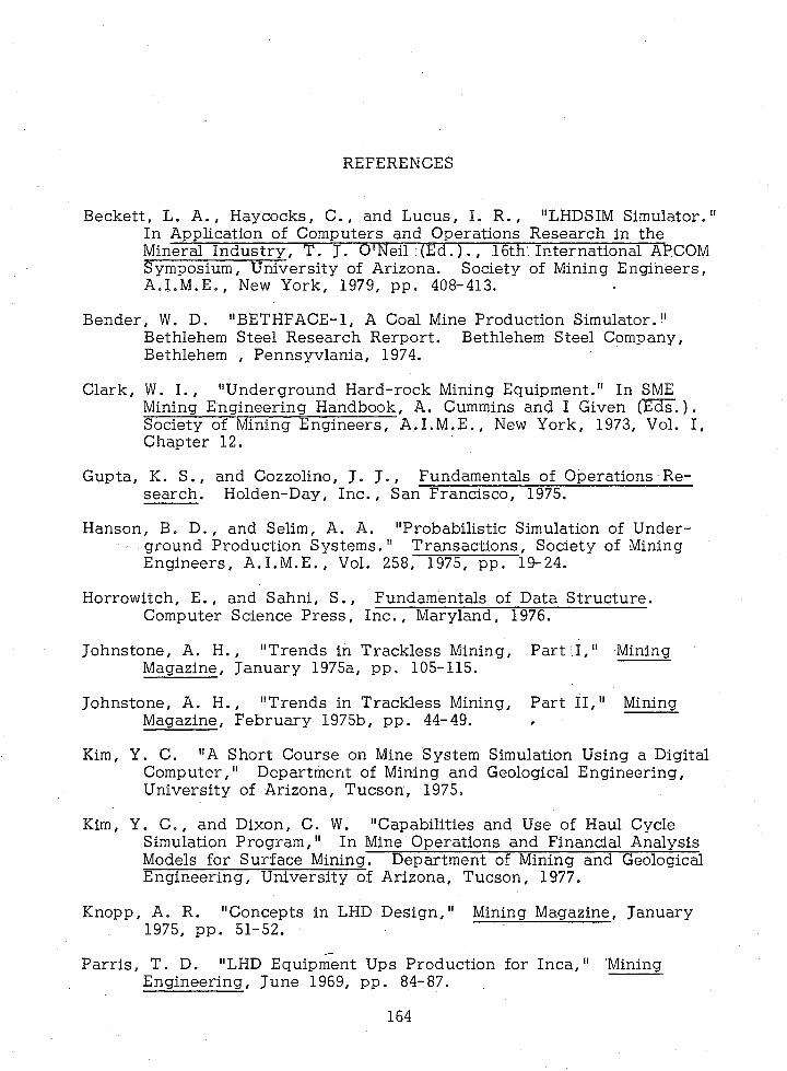
REFERENCES
Beckett, L. A ., Haycocks, C ., and Lucus, I. R ., "LHDSIM Simulator." In Application of Computers and Operations Research in the Mineral Industry, T. J. O'Neil (Ed.) . , 16th. International APCOM Symposium, University of Arizona. Society of Mining Engineers, A.I.M.E. , New York, 1979, pp. 408-413.
Bender, W. D. "BETHFACE-l, A Coal Mine Production Simulator."Bethlehem Steel Research Rerport. Bethlehem Steel Company, Bethlehem , Pennsyvlania, 1974.
Clark, W. I . , "Underground Hard-rock Mining Equipment." In SMEMining Engineering Handbook, A. Cummins and I Given (Eds.). Society of Mining Engineers, A.I.M.E. , New York, 1973, Vol. I, Chapter 12.
Gupta, K. S ., and Cozzolino, J. J . , Fundamentals of Operations Research. Holden-Day, Inc. , San Francisco, 1975.
Hanson, B. D . , and Selim, A. A. "Probabilistic Simulation of Underground Production System s." Transactions, Society of Mining Engineers, A.I .M.E. , Vol. 258, 1975, pp. 19-24.
Horrowitch, E ., and Sahni, S ., Fundamentals of Data Structure. Computer Science Press, Inc. , Maryland, 1976.
Johnstone, A. H ., "Trends in Trackless Mining, Part 11," Mining Magazine, January 1975a, pp. 105-115.
Johnstone, A. H ., "Trends in Trackless Mining, Part II," Mining Magazine, February 1975b, pp. 44-49.
Kim, Y. C. "A Short Course on Mine System Simulation Using a Digital Computer," Department of Mining and Geological Engineering, University of Arizona, Tucson, 1975.
Kim, Y. C ., and Dixon, C. W. "Capabilities and Use of Haul CycleSimulation Program," In Mine Operations and Financial Analysis Models for Surface Mining. Department of Mining and Geological Engineering, University of Arizona, Tucson, 1977.
Knopp, A. R. "Concepts in LHD Design," Mining Magazine, January 1975, pp. 51-52.
Parris, T. D. "LHD Equipment Ups Production for In ca ," 'Mining Engineering, June 1969, pp. 84-87.
164

165
P re laz , L . J . , Socronko, P. T . , Bucklen, E. P . , and Lucas, J . R ., "Optimization of Underground Mining." U.S. Office of Coal Research, R & D Report No. 6, 1964.
Sanford , L. R . , and Bloom, D . , "Simulation of LHD Operat ions ." In A Directory of Computer Programs Applicable to U .S . Mining Practices and Problems. Final Report on Contract No. G0264026, U.S. Bureau of Mines. Universi ty of Wisconsin-Platteville, Department of Mining Engineering, 1977, p. 267.
Suboleski, S. C . , and Weyher, L. H. E . , "Planning of Underground Material ." In Computer Methods for the 80's in the Mineral I n d u s t r y , A. Weiss (E d . ) . Society of Mining Engineers ,A . I . M . E . , New York, 1979, pp. 457-487.


