
Columbia University
Department of Economics Discussion Paper Series
Tests for Endogeneity and Instrument Suitability
Phoebus J. Dhrymes
Discussion Paper No.: 0203-21
Department of Economics Columbia University New York, NY 10027
August 2003

Tests for Endogeneity and Instrument
Suitability∗
PHOEBUS J. DHRYMES
Columbia University
June 9, 2003
Abstract
This paper deals with two alternatives to the so-called Hausmantest for the exogeneity of instruments, in the context of a model whereone or more explanatory variables are possibly correlated with thestructural error. These two alternatives are at least as good or betterthan the Hausman test and are much simpler to carry out.
A small Monte Carlo study illustrates this result.(JEL C10, C30, C43)
Key Words: Hausman test, instrumental variables, residual cor-relation test.
∗ c©Phoebus J. Dhrymes, 2003An earlier version of this paper was delivered as the ASSET Lecture in the annualmeetings of the Association of Southern European Economic Theorists, Paphos Cyprus,November 1 and 2, 2002.I would like to thank Timothy McKenna for his excellent research assistance in program-ming and executing the Monte Carlo study.Preliminary material; not to be quoted or disseminated without permission of the author.
1
1 Introduction
In this paper we deal with the issue of how to determine whether in the
following simple model
yi = xi·β + ui, xik = zi·γ + vi, i = 1, 2, . . . n, (1)
xik is or is not endogenous or, more precisely, is or is not correlated with
the error term ui . In Eq. (1), xi· is a k -element row vector whose last
element, xk , is suspected to be endogenous, in the sense that it is correlated
with the structural error ui ; similarly, zi· is an m -element row vector
of “instruments”, which are asserted to be independent of the structural
errors ui and vi . The vectors wi· = (ui, vi) , i = 1, 2, . . . , n are asserted
to be independent identically distributed (i.i.d.) with mean zero and an
unrestricted positive definite matrix, i.e.
Ew′i = 0, Cov(w
′
i) = Σ =
[σ11 σ12
σ21 σ22
]> 0. (2)
The literature on this model has a long history because the possibility
that one or more of the explanatory variables in a regression model is cor-
related with the error term can arise for a number of reasons. The early
literature, Wald (1940), dealt with the simplest version of the model above
as an error in variables model. It was inspired by, and connected to, physical
science issues such as the Heisenberg uncertainty principle which introduces,
in scientific measurements, errors of observation. Wald solved this problem
by inventing the notion of instrumental variables although, at the time, he
was not aware of this concept per se and its other potential uses. Wald’s
solution1 noted that if one could rank the observations on the indepen-
dent variable by their true value, then one could consistently estimate the
parameters of the (regression) line, because a line is determined by two
points. Using this additional information one could select the two points
in such a way that the slope is well determined and converges to the true
slope, at least in probability. Berkson (1950) noted that OLS estimators
1For a discussion of Wald’s paper see Dhrymes (1978), pp. 245-47.
2

in such models would be consistent and unbiased if one assumes that the
scientist sets the values of the explanatory variable(s)-in fact, ensuring that
the standard assumptions of the general linear model hold. Durbin (1954)
notes that of course such a rationale may be fine in the natural sciences but
not in economics. He correctly saw the problem in its contemporary set-
ting, i.e. as an issue in simultaneous equations theory. In fact, he explicitly
introduced what has come to be known as the “Hausman” test. However,
at the time it was not well understood how to handle “excess” instruments,
and his “Hausman” statistic is not as efficient as one could make it. Wu
(1973) extended Durbin’s work and produced what has become known as
the “Hausman” test. Hausman (1978) has given a broader rationale for
such a test and gave several examples of its possible applications.2 Oddly
enough even though Durbin, Wu and Hausman all note that the crucial as-
pect of this problem is the relationship between the error terms in the two
equations, none make this the focal point of their analysis. By contrast, this
paper concentrates entirely on this facet and motivates tests on the basis of
this relationship only.
Faced with the model of Eq. (1), practitioners are likely to estimate the
parameters of the (first equation of the) model by “2SLS”.
The 2SLS procedure customarily employed in the applied literature re-
gresses, in the first stage, x·k on Z = (zi·) to obtain
γ = (Z ′Z)−1Z ′x·k, x·k = Zγ, v = x·k − x·k. (3)
One then defines X = (X1, x·k) , where X1 = (x·1, x·2, . . . , x·k−1) and
y = Xβ + u + βkv; (4)
in the second stage one obtains the 2SLS estimator of the structural para-
meter β as
β = (X ′X)−1X ′y = β + (X ′X)−1X ′[u + βkv]. (5)
2For a comment on the Hausman test, and its unreliability when applied to testingprior restrictions in structural (simultaneous) equations models, see Dhrymes (1994a);for a discussion of its general nature see Dhrymes (1994b), pp. 52-60 .
3

To justify, motivate, or compel estimation of parameters by “2SLS”, it
is a widespread practice in this literature to test for the endogeneity (or
exogeneity) of xk by the Hausman test.
It is also a widespread practice to divide the matrix of the “instruments”,
Z , as Z = (Z1, Z2) , where the two constituent matrices are of dimension
n×m1 and n×m2 , respectively. It is asserted that Z1 contains instruments
that are independent of the error term, but there is some doubt as to whether
Z2 has the same properties. The suitability of the instruments in Z2 is also
judged by means of the Hausman test, i.e. one obtains the estimators of Eq.
(1) by using Z and Z1 alone, and then obtains the “Hausman statistic”
based on the difference β(Z) − β(Z1) . One or more of these procedures is
recommended in widely used textbooks such as Greene (2000), Chapters 9
and 14, and Davidson and Mackinnon (1993), Chapter 7, pp. 240ff.
This author, Dhrymes (1994a), has pointed out that, in the context of a
complete system of equations for which the Hausman test was originally de-
vised, results obtained by the application of such test are model dependent,
and often unreliable. The problem is that the Hausman test does not have
a specific parametric hypothesis to test, the results are difficult to interpret
and in some instances prove to be quite unreliable when the null is false.
In this paper we shall devise appropriate tests to address both questions
noted above.
2 Testing for Exogeneity
2.1 Structured Models
Proceeding somewhat formally, notice that if we consider the equations of
Eq. (1) a complete model, a necessary and sufficient condition to obtain
consistent and efficient estimators of the underlying parameters by least
squares is that the system be simply recursive. If that holds and, in
addition, the distribution of the errors is jointly normal the resulting
estimators are also maximum likelihood (ML) estimators and will possess
the property of sufficiency.
4

The model as formulated above is simply recursive if and only if
σ12 = 0. (6)
Hence, the hypothesis of exogeneity may be formulated as
H0 : σ12 = 0
as against the alternative
H1 : σ12 6= 0 .
Under the assumption of normality the likelihood function is given by
L∗n(β, γ, Σ) = (2π)−n|Σ|−(n/2)e−(1/2)trΣ−1S, S =
[s11 s12
s21 s22
], (7)
where s11 = (y − Xβ)′(y − Xβ) , s12 = (y − Xβ)′(x·k − Zγ) , s21 = (s12)′ ,
s22 = (x·k − Zγ)′(x·k − Zγ) . There are two ways this test may be imple-
mented. We can employ the likelihood ratio test (LRT), or we can devise
a test based entirely on the null.
The LRT statistic is obtained as
λ =maxH0 L∗
n
maxH1 L∗n
. (8)
As is well known, under the null, the maximum likelihood (ML) estimator
of the parameters in question is the OLS estimator,
βOLS = (X ′X)−1X ′y, γ = (Z ′Z)−1Z ′x·k. (9)
Consequently,
σ11 =u′u
n, σ22 =
v′v
n, u = y − Xβ, v = x·k − Zγ, so that
maxH0
L∗n = [σ11σ22]
−(n/2)][(2π)−ne−n]. (10)
Under the alternative, the ML estimator of the underlying parameters is
the 3SLS estimator
δ3SLS =
(β
γ
)=
[σ11X ′X σ12X ′Z
σ21Z ′X σ22Z ′Z
]−1 [σ11X ′y + σ12X ′x·k
σ21Z ′y + σ22Z ′x·k
]. (11)
5

This is so “because” in this case the Jacobian of the transformation from
(ui, vi) to (yi, xik) is unity.3
Thus, under the alternative
maxH1
L∗n = [σ11σ22(1 − r2
12)]−(n/2)][(2π)−ne−n], r2
12 =σ2
12
σ11σ22(12)
and, consequently,
λ =
((σ11σ22)OLS
(σ11σ22)3SLS(1 − r212)
)−(n/2)
∼ (1− r212)
n/2, or r212 ∼ 1−λ2/n, (13)
which shows that the square of the correlation coefficient between the 3SLS
residuals of the first and second equation is a likelihood ratio ststistic.
What is suggested by the discussion above is that we may base the test of
exogeneity on the 3SLS residuals from the first equation and the generalized
least squares residuals from the second, using the sample covariance. It can
be easily shown that
v′GLSu3SLS√
n∼ v′u√
n− σ22(β − β)k(3SLS), (14)
and moreover that
v′OLSu2SLS√
n∼ v′u√
n− σ22(β − β)k(2SLS). (15)
Although, as seen from Eqs. (14) and (15) the results are somewhat
different when we use 2SLS residuals from the first equation and OLS resid-
uals from the second, we shall examine the test based on the two stage
least squares residuals from the first equation and the OLS residuals from
the second in order to conform with much of the empirical practice, even
3Actually, the simplification induced by the unit Jacobian is overstated above. TheML estimator in this case is the 3SLS estimator iterated to convergence, so thatthe entities σij , (normally) the 2SLS estimators, should be understood to be the 3SLSestimators of the covariance parameters. But this aspect plays no appreciable role in thediscussion to follow. For a more general discussion of the relation between 3SLS and MLestimators see Dhrymes (1973).
6
though the LRT requires the use of 3SLS residuals4 from the first and GLS
residuals from the second equation, i.e. we consider
uv√n
=1√n
u′[In − X(X ′X)−1X ′][In − Z(Z ′Z)−1Z ′]v, (16)
where X = (X1, x·k) , x·k = Z(Z ′Z)−1Z ′x·k . As it will turn out, the test
statistic in Eq. (16) has precisely the same limiting distribution as that in
Eq. (17) below, viz.
1√n
x′·ku = x′
·k[In − X(X ′X)−1X ′]u. (17)
Alternatively, we may estimate the model under the null, in which case
we find the OLS estimates of β and γ , obtain the residuals and then carry
out the test. The first procedure is a conformity test, i.e. we estimate
the parameters without imposing the restriction of the null and then we
ask whether the results conform to the requirements of the null.5 In the
second alternative we operate entirely under the null, i.e. we estimate all
parameters assuming the null to be true, and then ask whether the null is
supported by the evidence. We shall establish the properties of both tests.
2.2 Derivation and Properties of the Test Statistics
In this and subsequent sections certain matrices will recur frequently and
so we shall employ the following notation for ease of exposition. A matrix
of the form Q(Q′Q)−1Q′ , will be routinely denoted by
Pq = Q(Q′Q)−1Q′, (18)
it being a projection matrix,6 i.e. for any suitably dimensioned vector, y ,
Pqy gives the projection of y on the space spanned by the columns of Q .
4Notice that under the null 2SLS and 3SLS are asymptotically equivalent. See alsothe discussion in Appendix II.
5For reasons unclear to me such tests are referred to in the literature as Wald tests.6For a discussion of the projection theorem see, e.g. Dhrymes (1998), Chapter 2.
7

Because in what follows a certain problem will recur frequently we examine
the issue in question before we proceed. Consider the entities
v′Pxu, v′Pzu, v′Pxu, v′X(X ′X)−1X ′u, v′X(X ′X)−1X ′u.
Under the null, all of these entities upon division by√
n , converge to zero
at least in probability. Under the alternative, however, their behavior is
quite different. Thus,
1√n
v′PxuP→ 0,
1√n
v′PzuP→ 0,
1√n
v′Pxud→ ±∞,
1√n
v′X(X ′X)−1X ′ud→ σ12e
′·kB
X ′u√n
, B =
(X ′X
n
)−1
1√n
v′X(X ′X)−1X ′ud→ σ12e
′·kB
X ′v√n
, (19)
where e·k is a k -element column vector all of whose elements are zero
except for the last, which is unity.
The residuals from the 2SLS procedure are given by
u = y − Xβ = u − X(β − β)
= u − X(X ′X)−1X ′[u + βkv]
= [I − X(X ′X)−1X ′]u. (20)
The last equality follows because
Z = (X1, P ), X1 = ZI∗k−1, I∗
k−1 = (Ik−1, 0)′, X = Z(I∗k−1, γ),
so that X ′v = 0 .
8

The OLS residuals from the first stage are evidently given by
v = [I − Pz]v. (21)
It may be shown by direct computation that, under the null,
1√n
v′u =1√n
v′[I − Pz − (0, v)(X ′X)−1X ′]u, (22)
because PzX = X . Moreover,
1
nv′(I − Pz)v
P→ σ22,
so that the quantity in the right member of Eq. (11) behaves like
1√n
v′u ∼ 1√n
(v − s)′u, where (23)
s′ = σ22(B21, B22)X′,
[B11 B12
B21 B22
]= B. (24)
Under the null, this a sequence of independent non-identically distributed
random variables with mean zero and variance
φi =E[(vi − si)ui]2 = E[v2
i u2i − 2siviu
2i + s2
i u2i ]
=E[v2i u
2i ] + E[s2
i u2i ] = σ11σ22 + σ11s
2i ;
σ11ω = limn→∞
n∑
i=1
1
nφi = σ11σ22[1 + σ22B22]. (25)
The derivation of the results above assumes that the joint distribution of u
and v is symmetric (which ensures that odd moments vanish) and normal
which, under the null, ensures that u and v are mutually independent.
Moreover, the Lindeberg condition is satisfied, and hence by the Linde-
berg CLT, see Dhrymes (1989), p. 271, we conclude that under the null
1√n
v′ud→ N(0, σ11ω), ω = σ22[1 + σ22(Rz − Rx1)
−1]. (26)
9

The entity in square brackets in the last equation of Eq. (14)is found as
follows:
plimn→∞
1
ns′s = plim
n→∞
1
n
(σ2
22(B21, B22)
(X ′X
n
)(B21, B22)
′)
= σ222 plim
n→∞
(1
n[x′
·kxk − x·kPx1x·k])−1
= σ222(Rz − Rx1)
−1,
because Px1Pz = Px1 , and Rz, Rx1 are, respectively, the mean sum of re-
gression squares in the regression of x·k on Z and X1 . Thus, the statistic7
tn =v′u√
nσ11σ22[1 + σ22B22]
d→ N(0, 1), (27)
may be used to test the hypothesis of exogeneity, where
σ11 =1
nu′u, σ22 =
1
nv′v,
B−122 =
1
nx′·kx·k −
x′·kX1
n
(X ′
1X1
n
)−1X ′
1x·k
n= Rz − Rx1 , (28)
where Rz, Rx1 are, respectively, the means of the regression sum of squares
in the regression of x·k on Z and X1 .
A variant of this test, i.e. a direct test that xk is correlated with the
structural error, is obtained by considering the entity
1√n
x′·ku. (29)
This test is asymptotically and numerically identical with the previous test,
as will be readily demonstrated by noting that
x·k = x·k + v, x′·ku = 0, so that x′
·ku = v′u.
7Note that, to avoid notational clutter, we use the symbol(s) Bij , i, j = 1, 2 to meanboth the elements of the block matrix (X ′X/n)−1 , as well as their respective limits.Similarly for the symbols Bij and their relation to (X ′X/n)−1 .
10
Hence, a test can be carried out through the statistic above, viz.
tn =x′·ku√
n[σ11σ22(1 + σ22B22)]
d→ N(0, 1). (30)
The alternative test, based entirely on the null, uses the residuals of the OLS
regressions from both equations, viz. u = (I − Px)u and v = (I − Pz)v to
form the statistic
1√n
v′u =1√n
v′(I − Pz)(I − Px)u. (31)
Employing precisely the same argument as above, we establish that
1√n
v′u∼ 1√n
(v − s∗)′u =1√n
n∑
i=1
(vi − s∗i )ui,
s∗′ = σ22e′·kBX ′, B =
(X ′X
n
)−1
. (32)
To determine its limiting distribution we note that
s∗i = σ22e′·kBx′
i· + σ22B22vi, X = (X1, Zγ) (33)
and, consequently,
vi − s∗i = (1 − σ22B22)vi − σ22e′·kBx′
i
φi = E[(vi − s∗i )ui]2 = (1 − σ22B22)
2σ11σ22 + σ11σ222e
′·kBx′
i·xi·Be·k
σ11ω1 = limn→∞
1
n
∞∑
i=1
φi = σ11σ22[1 − σ22B22]. (34)
By the Lindeberg CLT it follows that
1√n
v′ud→ N(0, σ11ω1), (35)
where
ω1 = σ22[1 − σ22B22],
[B11 B12
B21 B22
], B−1
22 =1
n[x′
·k(I − Px1)x·k]. (36)
11
Therefore a test of the hypothesis of exogeneity can be carried out through
the test statistic
t(1)n =v′u√
nσ11σ22(1 − σ22B22)
d→ N(0, 1). (37)
Remark 1. Notice that the estimator σ211 is based on the OLS resdiuals
from the structural equation and that the test statistic above is not of the
same form as that of Eq. (27), due to the fact that B22 ≥ B22 . Notice
further that B−122 is the mean sum of the squared residuals in the
regression of x·k on X1 .
2.3 Unstructured Models
Suppose, now, that in Eq. (1) we do not have a complete model but we
suspect that, either through measurement error, omitted variable, or simul-
taneity, the variable xk may be correlated with the structural error u . The
difference between this case and the earlier one is that a precisely specified
set of instruments is not available, and there is no precise specification for
the error vector v . Rather, there is under consideration one (or more)
matrix of instruments, W1 = (X1, P1) , whose elements are asserted to be
independent of the structural error u , and the structural parameter vector
β is to be estimated by instrumental variables (IV) methods. Following the
procedure given initially in Dhrymes (1969) and applied subsequently in
similar contexts by Amemiya (1974), Jorgenson and Laffont (1974), Hansen
(1982), inter alia, put
R1R′1 = W ′
1W1 (38)
and consider
R−11 W ′
1y = R−11 W ′
1Xβ + R−11 W ′
1u. (39)
As is well known, see Dhrymes (1970), pp. 302-303, 2SLS (OLS) is the opti-
mal IV estimator in the context of the transformed model of Eq. (28), when
the admissible class of instruments is W1A , where A is an arbitrary non-
singular matrix. The OLS estimator of β in the context of the transformed
12
model in Eq. (28) is
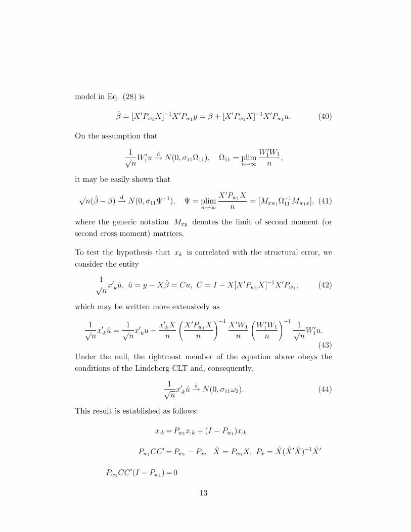
β = [X ′Pw1X]−1X ′Pw1y = β + [X ′Pw1X]−1X ′Pw1u. (40)
On the assumption that
1√n
W ′1u
d→ N(0, σ11Ω11), Ω11 = plimn→∞
W ′1W1
n,
it may be easily shown that
√n(β − β)
d→ N(0, σ11Ψ−1), Ψ = plim
n→∞
X ′Pw1X
n= [Mxw1Ω
−111 Mw1x], (41)
where the generic notation Mxy denotes the limit of second moment (or
second cross moment) matrices.
To test the hypothesis that xk is correlated with the structural error, we
consider the entity
1√n
x′·ku, u = y − Xβ = Cu, C = I − X[X ′Pw1X]−1X ′Pw1, (42)
which may be written more extensively as
1√n
x′·ku =
1√n
x′·ku − x′
·kX
n
(X ′Pw1X
n
)−1X ′W1
n
(W ′
1W1
n
)−11√n
W ′1u.
(43)
Under the null, the rightmost member of the equation above obeys the
conditions of the Lindeberg CLT and, consequently,
1√n
x′·ku
d→ N(0, σ11ω2). (44)
This result is established as follows:
x·k =Pw1x·k + (I − Pw1)x·k
Pw1CC ′ =Pw1 − Px, X = Pw1X, Px = X(X ′X)−1X ′
Pw1CC ′(I − Pw1) = 0
13
(I − Pw1)X =(0, v), v = (I − Pw1)x·k
(I − Pw1)CC ′(I − Pw1) = I − Pw1 + (I − Pw1)X(X ′X)−1X ′(I − Pw1)
Pw1CC ′Pw1 =Pw1 − Px, so that
ω2 =plimn→∞
1
nx′·k(Pw1 − Px)x·k + σ∗
22 + B22σ∗222 ,
σ∗22 =plim
n→∞
x′·k(I − Pw1)x·k
n. (45)
To show that, mutatis mutandis, ω2 is the “same” as ω in the first two
tests, note that
x′·k(Pw1 − Px)x·k = 0, (46)
and further note that
x′·kX = x′
·kX + (0, v∗′v∗),
because
x′·k(Pw1 − Px) = x′
·k − x′·kX(X ′X)−1X ′ = x′
·k − e′·kX′ = 0, (47)
and identify σ22 with σ∗22 . It follows, then, that
t(2)n =x′·ku√
nσ11σ∗22[1 + σ∗
22B22]→ N(0, 1) (48)
is a suitable test statistic for testing the hypothesis that x·k is exogenous,
when a complete model s not specified. In the preceding
σ11 =u′u
n, σ∗
22 =x′·k(I − Pw1)x·k
n.
In this section we have proved the following:
Proposition 1. Consider the model in Eq. (1), a complete model under
the assumptions
A1 wi· = (ui, vi) is a sequence of i.i.d. random vectors with mean zero
and covariance matrix Σ > 0 .
14

A2 The variables in the vector zi· , as well as the first k − 1 elements of
the vector xi· , are independent of the vector wi· , but the last element
of xi· , xk , may be correlated with ui , i.e. it may be endogenous.
A test of the hypothesis that xk is exogenous is equivalent to the test
that σ12 = 0 . A test of this hypothesis may be carried out using the test
statistic(s) in Eq. (27), or, equivalently, Eq. (30). An alternative test,
based entirely on the null, may be carried out based on the statistic in Eq.
(37).
If a complete model is not available, so that we deal only with the first
equation of Eq. (1), but we have an instrumental matrix W1 = (X1, S1) , a
test of the exogeneity of xk may be based on the test statistic of Eq. (48).
2.4 Testing for the Exogeneity of Instruments
Actually Used
Having obtained the estimator dealt with immediately above, we may wish
to test whether the matrix W1 contains elements that are indeed indepen-
dent of the structural error u . To this end consider the entity
1√n
W ′1u = G
1√n
W ′1u, G = I − W ′
1X
n
(X ′Pw1X
n
)−1X ′W1
n
(W ′
1W1
n
)−1
.
(49)
Under the null, the entity above obeys the conditions of the Lindeberg
CLT and thus
1√n
W ′1u
d→ N(0, σ11Φ1), Φ1 = plimn→∞
GW ′
1W1
nG′. (50)
The expression above can be considerably simplified by direct manipulation
to show that
GW ′
1W1
nG′ =
W ′1W1
n− W ′
1X
n
(X ′Pw1X
n
)−1X ′W1
n. (51)
To show that the distribution is or is not degenerate, we need to show that,
for all n ≥ k+m , the matrix in Eq. (50) is positive semi-definite or positive
15
definite, respectively. To this end apply the simultaneous decomposition
theorem, see Dhrymes (2000), p. 87 and note that the difference may be
expressed as
GW ′
1W1
nG′ = R1
[0 0
0 Im−1
]R′
1, whereW ′
1W1
n= R1R
′1. (52)
This is so because W1 is of dimension n×k+m−1 , and the characteristic
roots of the second matrix of the difference (in Eq. (50), in the metric
of the first matrix of the difference consist of k unities and m − 1 zeros.
Thus, the matrix Φ1 is positive semi-definite of rank m − 1 .
Remark 2. The result above means that we cannot test for the exogeneity
of all instruments; it is similar, mutatis mutandis, to our inability to test
for the validity of all prior restrictions in a complete simultaneous equations
system, see Dhrymes (1994a).
Let Sj be a selection matrix, i.e. a matrix that contains m1−1 ≥ j of the
columns of the k + m1 − 1 - dimensioned identity matrix, Ik+m1−1 . Then,
S ′jW
′1u
nd→ N(0, σ11S
′jΦ1Sj). (53)
Consequently, we can test the hypothesis using the statistic below,
tj =[S ′
ju]′[S ′jG(W ′
1W1/n)G′Sj]−1[S ′
ju]
u′u/nd→ χ2
m−1. (54)
This statistic is simple to compute since all entities, save the selection ma-
trix, are routinely computed in the process of obtaining the estimator, and
the test is the precise analog of the test for (some or all) over-identifying
restrictions in the general linear structural econometric model (GLSEM)
given in Dhrymes (1994).
Remark 3. The fact that Φ1 is of rank m − 1 means that at least one
m − 1 dimensional sub-matrix is nonsingular. But there may very well be
several. This means that more than one group of m − 1 instruments may
be tested for exogeneity. From the point of view of the researcher it may not
16
be desired to test for the exogeneity of variables in the matrix X1 , only for
those in P1 . However, in the context we have created above it is certainly
possible to do so for both, provided n − k ≥ k − 1 and n − k ≥ m1 − 1 .
2.5 Testing for the Exogeneity of
Contemplated Instruments
In the context of the discussion of the previous section, suppose we obtained
the IV estimator using the instrumental matrix W1 , but now we wish to
test for the exogeneity of possible instruments we did not use, say those
contained in the matrix P2 , where P2 is n × m2 of rank m2 .
This problem may be solved by the same method as above, assuming
that we are satisfied that W1 is an admissible instrumental matrix, and
that the resulting estimator is consistent. To this end consider the entity
1√n
P ′2u =
1√n
P ′2u−
P ′2X
n
(X ′Pw1X
n
)−1X ′W1
n
(W ′
1W1
n
)−1W ′
1u√n
=1√n
P ′2Cu,
(55)
where C = I − X(X ′Pw1X/n)−1X ′Pw1 .
By the Lindeberg CLT
1√n
P ′2u
d→ N(0, σ11Φ2), where (56)
Φ2 = plimn→∞
1
nP ′
2CC ′P2.
To evaluate Φ2 , we note that
P2 = Pw1P2 + (I − Pw1)P2 (57)
Pw1CC ′ = Pw1 − Px, X = Pw1X, Px = X(X ′X)−1X ′
Pw1CC ′(I − Pw1)= 0
(I − Pw1)X = (0, v), v = (I − Pw1)x·k
17

(I − Pw1)CC ′(I − Pw1)= I − Pw1 + (I − Pw1)X(X ′X)−1X ′(I − Pw1)
Pw1CC ′Pw1 = Pw1 − Px, so that
Φ2 = plimn→∞
1
nP ′
2(Pw1 − Px)P2 + B22ξξ′, ξ = plim
n→∞
P ′2v
n.
Since B22ξξ′ is a positive semi-definite matrix of rank 1, and Px is an
idempotent matrix of rank n− k −m + 1 it follows that the rank of Φ2 is
m2 , provided n−k−m+1 ≥ m2 . In such a case, all additional instruments
(i.e. the variables contained in P2 ) can be tested for instrument suitability,
by means of the statistic
tn =1
n(P ′
2u)′Φ−12 (P ′
2u)d→ χ2
m2, (58)
where Φ2 is a consistent estimator of Φ2 . Any subset of the instruments
may be tested by the same method, using a suitably dimensioned selection
matrix
3 Power of Tests: Limiting Distribution
under the Alternative
3.1 Structured Models
We first examine the tests exhibited in Eqs. (27) and (37). In view of Eq.
(8), we have
v′u√n
=1√n
v′[I − X(X ′X)−1X ′]u − 1√n
(v′Pzu − v′Pxu)
∼ 1√n
v′[I − X(X ′X)−1X ′]u
=1√n
v′(I − Px)u − v′v
ne′·k
(X ′X
n
)−11√n
X ′u
∼ 1√n
(v − s)′u =1√n
n∑
i
(vi − si)ui. (59)
18

where si = σ22e′·kBx′
i· . However, the summands, (vi − si)ui do not have
mean zero under the alternative; their mean is σ12 . Thus, we need to
considerv′u√
n−√
nσ12 ∼1√n
n∑
i=1
[(vi − si)ui − σ12)], (60)
which obeys the conditions of the Lindeberg CLT. Consequently, using the
same arguments as before, we conclude that
v′u√n−√
nσ12d→ N(0, ω∗), ω∗ = σ11σ22[1 + σ22B22] + σ2
12.8 (61)
Thus, under the alternative
H1 : σ12 = φ∗√
n,
the test statistic(s) in Eqs. (27) and (37) obey
t2nd→ χ2(λ), λ =
φ∗2
2σ11σ22(1 + σ22B22). (62)
Turning now to the test (statistic) of Eq. (37) and repeating the steps
leading to Eqs. (31) through (34) we see that under the alternative
E(vi − s∗i )ui = (1 − σ22B22)σ12. (63)
Thus,
1√n
v′u−(1−σ22B22)√
nσ12 ∼1√n
n∑
i=1
[(1−σ22B22)(viui−σ12)−σ22e′·kBx′
i·ui],
(64)
and consequently
1√n
v′u − (1 − σ22B22)√
nσ12d→ N(0, σ11ω). (65)
8In fact, the last term, σ212 , should not be there because it results when we sum,
divide by n and take the limit of the variances of the summands. Since under thealternative σ12 = φ∗/
√n , it follows that upon taking limits ω∗ = σ11ω as in Eq. (26).
19

But this implies that the test statistic in Eq. (37) obeys under the alter-
native
t(1)n =v′u√
nσ11σ22(1 − σ22B22)
d→ χ2(λ1), λ1 =φ∗2(1 − σ22B22)
2σ11σ22
(66)
Turning now to the entity in Eq. (42) and the test (statistic) in Eq. (48),
we consider the limiting distribution under the alternative.
Reamrk 4. In dealing with this issue under the null, we had concealed the
fact that the standard assumptions made in this context are not sufficient
to enable formal derivations. It is not enough merely to say that we have
some instruments which are independent of the structural error u . More is
required as will become apparent when the argument unfolds.
Rewrite Eq. (43) as
1√n
x′·ku =
1√n
x′·ku − 1√
n
(x·kX
n
)(X ′Pw1X
n
)−1
X ′Pw1u, (67)
and note that
x′·kX = x′
·kPw1X + x′·k(I − Pw1)X = x′
·kPw1X + e′·kv′v, (68)
where v = (I − Pw1)x·k . Thus, the statistic of Eq. (48) behaves like (upon
taking a certain probability limit)
1√n
x′·ku ∼ 1√
nv′u − 1√
ndu, d = σ∗
22e′·k
(X ′Pw1X
n
)−1
X ′Pw1. (69)
Remark 5. At this stage the need for more precise specification becomes
evident, because what we have assumed until now is that v is the orthog-
onal complement of the projection of x·k on the space spanned by W1 .
To treat the elements of v as random variables with the properties (once
removed) required for the invocation of a CLT is almost tantamount to sta-
ting that x·k = W1γ+v , in which case we should have a complete model, as
20

in the case of the first test we considered. In fact, this must be the implicit
assumption made by practitioners who employ such techniques.
Be that as it may, we note that under the alternative
1√n
x′·ku ∼ 1√
n
n∑
i=1
[viui − diui], (70)
and the individual terms of the sum do not have mean zero. Thus, if we
mimic the previous derivations we are led to consider
1√n
x′·ku −
√nσ12 ∼
1√n
n∑
i=1
[(viui − σ12) − diui], (71)
which will obey the conditions of the Lindeberg CLT, whence we conclude
1√n
x′·ku −
√nσ12
d→ N(0, σ11σ∗22[1 + σ∗
22B22]), (72)
[t(2)n ]2d→ χ2(λ2), λ2 =
φ∗2
2σ11σ∗22[1 + σ∗
22B22]. (73)
3.2 Unstructured Models
Here we examine, under the alternative, the limiting distribution of the
entity in Eq. (38) and, hence, that of the test statistic in Eq. (43).
If we consider the vector ξi· = (ui, wi1·) , where its second component
it the i th row of W1 –and thus a k + m -dimensioned random vector with
mean, say zero for convenience, and covariance matrix
Cov(ξi·) = Σ =
[σ11 σ1·
σ·1 Σ22
], (74)
we may, with little loss of relevance, assume that
Σ22 = plimn→∞
1
nW ′
1W1 (75)
and state the hypotheses under consideration
H0 : σ·1 = 0
as against the alternative H1 : σ·1 = 1√nφ∗
3 ,
21

where φ∗1 is a non-zero vector.
Proceeding as before, we consider
1√n
W ′1u −
√nσ·1 =
1√n
[n∑
i=1
(w′i1·ui − σ·1]. (76)
The summands are a sequence of independent random vectors obeying the
Lindeberg CLT conditions; moreover, the covariance matrix of the typical
summand is
Cov[w′i1·ui − σ·1] =E
(w′
i1·u2i w
′i1· − [w′
i1·ui]σ′·1 − σ·1[w
′i1·ui]
′ + σ·1σ′·1
)
=σ11Σ22 + 2σ·1σ′·1 − 2σ·1σ
′·1 + σ·1σ
′·1
=σ11Σ22 + σ·1σ′·1. (77)
We therefore conclude that, under the alternative,
1√n
W ′1u −
√nσ·1
d→ N(0, σ11Φ1), (78)
and, consequently that under the alternative
1√n
W ′1u
d→ N(φ∗3, σ11Φ1). (79)
An immediate consequence of the preceding is that the test statistic of Eq.
(54) converges in distribution to a non-central chi-square distribution, i.e.
under the alternative
tj =[S ′
ju]′[S ′jG(W ′
1W1/n)G′Sj]−1[S ′
ju]
u′u/nd→ χ2
m−1((λ3)),
λ3 =1
2φ∗′
3 (σ11Φ1)−1φ∗
3. (80)
The discussion with respect to contemplated instruments is quite similar
to that for instruments already employed, except that now we rule out
correlation between the instruments already used and the structural error
term. The only question is whether the contemplated instruments exhibit
22

such a feature. For the current discussion it will be convenient if we recast
Eq. (55) as
1√n
P ′2u=
n∑
i=1
[p′i1· − Mw′i1·]ui,
M =P ′
2X
n
(X ′Pw1X
n
)−1X ′W1
n
(W ′
1W1
n
)−1W ′
1u√n
. (81)
Since MP→ M , we see that
1√T
P ′2u ∼
n∑
i=1
[p′i1· − Mw′i1·ui, (82)
and the summands under the null are independent random vectors with
mean
Epı2·ui = σ·1, Cov(pı1·ui) = σ11Σ22 + σ·1σ′·1. (83)
In deriving this result, we have defined the vector ζi· = (ui, pi2·) we have
put
Cov(ζi·) =
[σ11 σ′
·1
σ·1 Σ22
](84)
and assumed that Σ22 = plimn→∞(P ′2P2/n) .
Since, under the alternative, Ep′i2ui = σ·1 6= 0 , we conclude that under
the alternative
H1 : σ·1 = 1√nφ∗4 ,
1√n
P ′2u
d→ N(φ∗4, σ11φ2) (85)
and, consequently, the test statistic in Eq. (58) obeys,
tn =1
n(P ′
2u)′Φ−12 (P ′
2u)d→ χ2
m2(λ4), (86)
where
λ4 =1
2φ∗′
4 (σ11Φ2)−1φ∗
4.
23
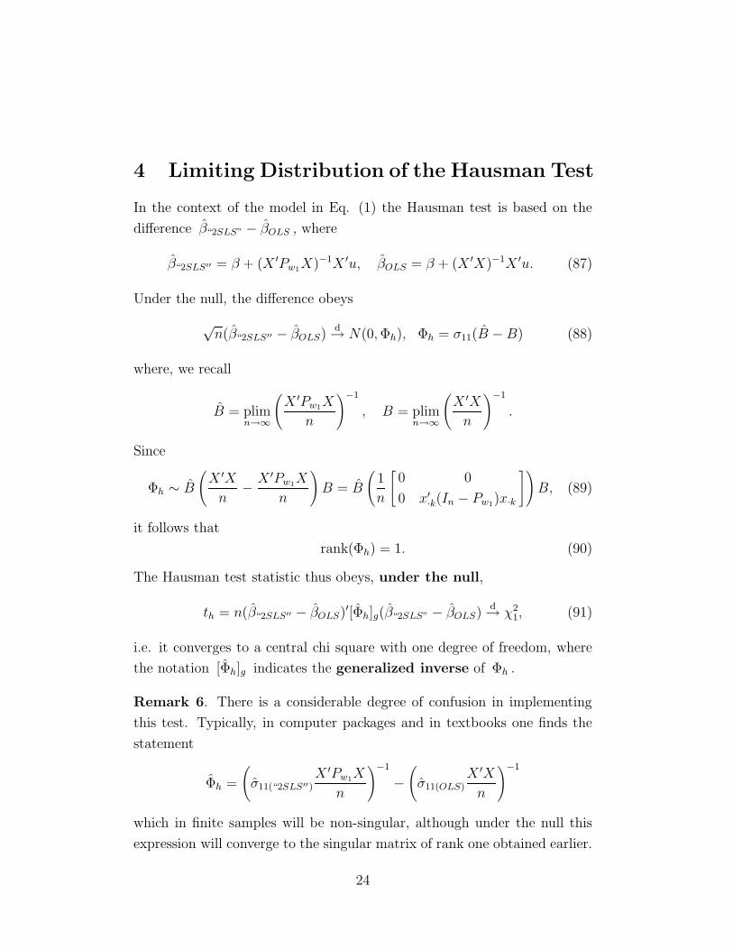
4 Limiting Distribution of the Hausman Test
In the context of the model in Eq. (1) the Hausman test is based on the
difference β“2SLS” − βOLS , where
β“2SLS′′ = β + (X ′Pw1X)−1X ′u, βOLS = β + (X ′X)−1X ′u. (87)
Under the null, the difference obeys
√n(β“2SLS′′ − βOLS)
d→ N(0, Φh), Φh = σ11(B − B) (88)
where, we recall
B = plimn→∞
(X ′Pw1X
n
)−1
, B = plimn→∞
(X ′X
n
)−1
.
Since
Φh ∼ B
(X ′X
n− X ′Pw1X
n
)B = B
(1
n
[0 0
0 x′·k(In − Pw1)x·k
])B, (89)
it follows that
rank(Φh) = 1. (90)
The Hausman test statistic thus obeys, under the null,
th = n(β“2SLS′′ − βOLS)′[Φh]g(β“2SLS” − βOLS)d→ χ2
1, (91)
i.e. it converges to a central chi square with one degree of freedom, where
the notation [Φh]g indicates the generalized inverse of Φh .
Remark 6. There is a considerable degree of confusion in implementing
this test. Typically, in computer packages and in textbooks one finds the
statement
Φh =
(σ11(“2SLS′′)
X ′Pw1X
n
)−1
−(σ11(OLS)
X ′X
n
)−1
which in finite samples will be non-singular, although under the null this
expression will converge to the singular matrix of rank one obtained earlier.
24

It would appear that, in the spirit of asymptotic theory, the expression
above “ought” to be written as
Φh = σ11(“2SLS′′)
(
X ′Pw1X
n
)−1
−(
X ′X
n
)−1 , (92)
which, mimics the asymptotic rank for all sample sizes and, in any event,
converges to the desired entity both under the null and under the alternative.
Under the alternative, the OLS estimator is inconsistent, and its inconsis-
tency is given by
plimn→∞
(βOLS − β) = σ12Be·k. (93)
It may further be shown that under the alternative
√n(β“2SLS′′ − βOLS) −
√nσ12Be·k
d→ N(0, Φh), (94)
or that √n(β“2SLS′′ − βOLS)
d→ N(φ∗Be·k, Φh) (95)
and, consequently, that
thd→ χ2
1(λh), λh =1
2φ∗2e′·kB[Φh]gBe·k. (96)
The distributions of the other variants of the Hausman test, noted at
the beginning, are similarly obtained and, thus, will not be pursued here.
25
BIBLIOGRAPHY
Amemiya, T. (1974), “The nonlinear least squares estimator”, Journal of
Econometrics, vol. 2, pp. 105-110.
Berkson, J. (1950), “Are there two regressions?” Journal of the American
Statistical Association, vol. 47, pp.164-180
Davidson, R and J. MacKinnon (1993), Estimation and Inference in Econo-
metrics, New York: Oxford University Press.
Dhrymes, P. J. (1969), “Alternative asymptotic tests of significance and
related aspects of 2SLS and 3SLS estimated parameters”, The Review of
Economic Studies, vol. 36, pp. 213-236.
Dhrymes, P. J. (1970), Econometrics: Statistical Foundations and Applica-
tions, New York: Harper and Row.
Dhrymes, P. J. (1973), ‘Small Sample and Asymptotic Relations between
Maximum Likelihood and Three Stage Least Squares Estimators”, Econo-
metrica, vol. 41, pp. 357-364.
Dhrymes, P.J.(1978), Introductory Econometrics, New York: Springer Ver-
lag.
Dhrymes, P. J. (1994a), “Specification tests in simultaneous equations sys-
tems”, Journal of Econometrics, pp. 45-76.
Dhrymes, P. J. (1994b),Topics in Advanced Econometrics: vol. II Linear
and Nonlinear Simultaneous Equations, New York: Springer Verlag.
Dhrymes, P. J. (1989), Topics in Advanced Econometrics: Probability Foun-
dations, New York: Springer Verlag.
Dhrymes, P. J. (1998), Time Series, Unit Roots and Cointegration, San
Diego: Academic Press.
Dhrymes, P. J. (2000), Mathematics for Econometrics, Third Edition, New
York: Springer Verlag
26
Durbin, J. (1954), “Errors in Variables”, Review of the International Sta-
tistical Insitute, vol. 22, pp. 23-32.
Greene, W. H. (2000), Econometric Analysis, Fourth Edition, Upper Saddle
River: Prentice Hall Inc.
Hansen, L. P. (1982),“Large Sample Properties of the Generalized Method
of Moments”, Econometrica, vol. 50, pp. 1029-1054.
Hausman, J. A. (1978),“Specification Tests in Econometrics”, Economet-
rica, vol. 46, pp. 1251-1271.
Jorgenson, D. and J. Laffont *1974), “Efficient Estimation of Nonlinear
Simultaneous Equations with Additive Disturbances”,Annals of Economic
and Social Measurement, vol. 3, pp. 615-640.
Reiersol, O. (1950), “Identifiability of a linear relation between variables
which are subject to error”, Econometrica, vol. 18, pp. 375-389.
Wald, A. (1940), “The fitting of straight lines if both variables are subject
to error”, Annals of Mathematical Statistics, vol. 11, pp. 284-300.
Wu, D. (1973), “Alternative Tests of Independence between Stochastic Re-
gressors and Disturbances”, Econometrica, vol. 41, pp.733-750.
27
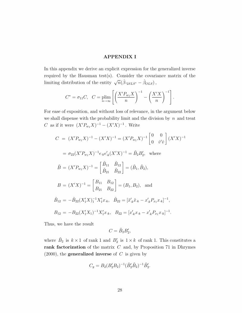
APPENDIX I
In this appendix we derive an explicit expression for the generalized inverse
required by the Hausman test(s). Consider the covariance matrix of the
limiting distribution of the entity√
n(β“2SLS” − βOLS) ,
C∗ = σ11C, C = plimn→∞
(
X ′Pw1X
n
)−1
−(
X ′X
n
)−1 .
For ease of exposition, and without loss of relevance, in the argument below
we shall dispense with the probability limit and the division by n and treat
C as if it were (X ′Pw1X)−1 − (X ′X)−1 . Write
C = (X ′Pw1X)−1 − (X ′X)−1 = (X ′Pw1X)−1
[0 0
0 v′v
](X ′X)−1
= σ22(X′Pw1X)−1e·ke
′·k(X
′X)−1 = B2B′2, where
B = (X ′Pw1X)−1 =
[B11 B12
B21 B22
]= (B1, B2),
B = (X ′X)−1 =
[B11 B12
B21 B22
]= (B1, B2), and
B12 = −B22(X′1X)−1
1 X ′1x·k, B22 = [x′
·kx·k − x′·kPx1x·k]
−1,
B12 = −B22(X′1X1)
−1X ′1x·k, B22 = [x′
·kx·k − x′·kPx1x·k]
−1.
Thus, we have the result
C = B2B′2,
where B2 is k × 1 of rank 1 and B′2 is 1× k of rank 1. This constitutes a
rank factorization of the matrix C and, by Proposition 71 in Dhrymes
(2000), the generalized inverse of C is given by
Cg = B2(B′2B2)
−1(B′2B2)
−1B′2.
28

Carrying out the requisite operations and defining ζ = (X ′1X1)
−1x·k , we
find
Cg =B−122
1
1 + ζ ′ζ
[ζζ ′ −ζ
−ζ ′ 1
]1
1 + ζ ′ζB−1
22 , and thus
C∗g =
1
σ11σ22
(B−1
22
1
1 + ζ ′ζ
)[ζζ ′ −ζ
−ζ ′ 1
](1
1 + ζ ′ζB−1
22
).
Inserting this representation in the non-centrality parameter of Eq. (96)
yields
λh =1
2φ∗2e′·kB[Φh]gBe·k =
1
2σ11φ∗2 x′
·k(Pw1 − Px1)x·k
x′·k(I − Px1)x·k
.
29

APPENDIX II
In this appendix we generalize the discussion based on Eqs. (1) and (2),
so that more than one right hand variables may be tested for exogeneity.
We find that the results obtained with a single potential endogenous right
hand variable carry over entirely, mutatis mutndis to the vector case. To
this end, consider
y·t = X1β(1) + X2β(2) + u, X2 = W1Γ + V,
where now X1 is n × k1 , X2 is n × k2 , k1 + k2 = k . Putting
x(2) = vec(X2), v = vec(V ), γ = vec(Γ),
we can rewrite the entire system compactly as
y = Xβ + u, x(2) = (Ik2 ⊗ W1)γ + v,
and a single observation as
yi − x(2)i· β(2) = x
(1)i· β(1) + ui, x
(2)i· = w
(1)i· Γ + vi·.
Under the standard assumptions (including joint normality of the errors)
we may write the likelihood function in terms of the errors as
L∗(u, V ; Σ) = (2π)−n(k2+1)/2|Σ|−(n/2)e−12trΣ−1S∗
, S∗ =
[u′u u′V
V ′u V ′V
].
Viewing the equation for a single observation as a transformation from
(ui, vi·)′ to (yi, x
2i·)
′ , we find that the Jacobian matrix is
J =
[1 −β ′
(2)
0 Ik2
],
so that the Jacobian of the transformation is |J | = 1 ; thus, the (log)
likelihood function of the observations is
L =−n(k2 + 1)
2ln(2π) +
n
2ln|Σ−1| − 1
2trΣ−1S, S =
[s11 s1·
s·1 S22
]
30

s11 = (y − Xβ)′(y − Xβ), s1· = (s12, s13, . . . , s1(k2+1))
s1j = (y − Xβ)′(x·k1+j−1 − W1γ·j−1), j = 2, 3, . . . , k2 + 1, s·1 = s′1·,
S22 = (sij), sij = (x·k1+i−1 − W1γ·i−1)′(x·k1+j−1 − W1γ·j−1), j = 2, 3, . . . , k2 + 1.
Differentiating with respect to Σ−1 yields
∂L
∂Σ−1=
n
2Σ − 1
2S = 0, or Σ =
1
nS.
Inserting this in the loglikelihood function we find the concentrated (log)
likelihood function
L(β, γ) = −n(k2 + 1)
2[ln(2π) + 1] +
n
2ln(n) − n
2ln|S|.
As we have done in the discussion surrounding Eq. (8), we note that
the LRT statistic is some function of the likelihood ratio (LR)
λ =maxH0 L∗
n
maxH1 L∗n
.
In this instance the null is that σ·1 = 0 , where
Σ =
[σ11 σ1·
σ·1 Σ22
].
We note thatΣ2 is k2 × k2 and thus σ·1 is k2 × 1 . Consequently, the LR
is given by
λ =
(|SH0||SH1|
)(−n/2)
=
(σ11|Σ22|σ11|Σ22|)
(1 − σ1·(σ11|Σ22|)−1σ·1
)−(n/2)
∼((1 − σ1·(σ11|Σ22|)−1σ·1
)(n/2)or
1 − λ(2/n) ∼ σ1·(σ11|Σ22|)−1σ·1.
If we use the sample analogs of these entities, we find
σ1·(σ11|Σ22|)−1σ·1 = u′V (u′uV ′V )−1V ′u,
31

which suggests the test statistic V ′u/√
n , where
u= y − Xβ3SLS = u − X(β3SLS − β),
V = X2 − W1Γ3SLS = V − W1(Γ3SLS − Γ).
We can use 3SLS (instead of ML) estimators because, as we pointed out
earlier, the Jacobian of the transformation is unity, and in such cases ML
and iterated 3SLS will coincide.
Consider now the statistic
1√n
V ′u =1√n
[V − W1(Γ3SLS − Γ)]′[u − X(β3SLS − β)],
which upon multiplication and taking (probability) limits reduces to
1√n
V ′u ∼ 1√n
V ′u − (0, Σ22)√
n(β3SLS − β).
But the second term may be easily shown to be (asymptotically) uncorre-
lated with the first and, thus, the covariance matrix of the limiting distri-
bution of the entity above is simply the sum of the covariance matrices of
the limiting distributions of the two terms, i.e.
1√n
V ′ud→ N(0, C), C = C1 + C2,
where, under the null, C1 = σ11Σ22 and C2 is the submatrix of the co-
variance matrix of the limiting distribution of β3SLS corresponding to its
subvector β(2) . To determine the limiting distribution of the 3SLS estima-
tor of β , write the system as
y = Xβ + u, x(2) = (Ik2 ⊗ W1)γ + v, γ = vec(Γ), v = vec(V ).
Let W ′1W1 = R1R
′1 , where R1 is a non-singular matrix; such a matrix
exists because W1 if of full (column) rank. Transform the system by pre-
multiplying the first equation be R−11 W ′
1 and the second by Ik2 ⊗ R−11 W ′
1
32
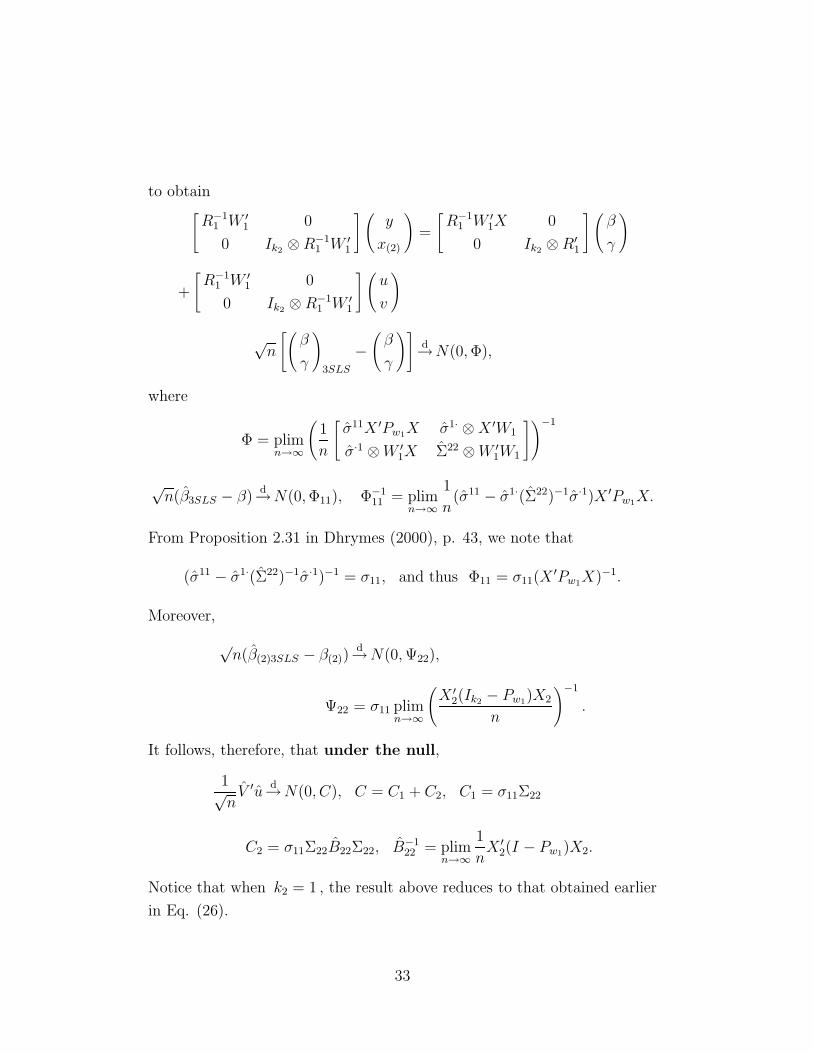
to obtain[R−1
1 W ′1 0
0 Ik2 ⊗ R−11 W ′
1
](y
x(2)
)=
[R−1
1 W ′1X 0
0 Ik2 ⊗ R′1
](β
γ
)
+
[R−1
1 W ′1 0
0 Ik2 ⊗ R−11 W ′
1
](u
v
)
√n
[(β
γ
)
3SLS
−(
β
γ
)]d→N(0, Φ),
where
Φ = plimn→∞
(1
n
[σ11X ′Pw1X σ1· ⊗ X ′W1
σ·1 ⊗ W ′1X Σ22 ⊗ W ′
1W1
])−1
√n(β3SLS − β)
d→N(0, Φ11), Φ−111 = plim
n→∞
1
n(σ11 − σ1·(Σ22)−1σ·1)X ′Pw1X.
From Proposition 2.31 in Dhrymes (2000), p. 43, we note that
(σ11 − σ1·(Σ22)−1σ·1)−1 = σ11, and thus Φ11 = σ11(X′Pw1X)−1.
Moreover,
√n(β(2)3SLS − β(2))
d→N(0, Ψ22),
Ψ22 = σ11 plimn→∞
(X ′
2(Ik2 − Pw1)X2
n
)−1
.
It follows, therefore, that under the null,
1√n
V ′ud→N(0, C), C = C1 + C2, C1 = σ11Σ22
C2 = σ11Σ22B22Σ22, B−122 = plim
n→∞
1
nX ′
2(I − Pw1)X2.
Notice that when k2 = 1 , the result above reduces to that obtained earlier
in Eq. (26).
33

To test the null hypothesis H0 : σ·1 = 0 , we may thus use the statistic
t2m =u′V√
n
[σ11Σ22(Ik2 + B22)Σ22
]−1 V ′u√n
d→ χ2k2
,
which is the multivariate generalization of the statistic given in Eq. (27).
Remark AII.1 The asymptotic equivalence between the 2SLS and 3SLS
estimators of β , in the context of this model, in part explains why in the
body of the paper we had dealt essentially with the “2SLS” estimator only.
34

APPENDIX III
In this appendix we report the results of a limited Monte Carlo study as
follows: The results of the Monte Carlo study are reported in the tables
below. They involve 10,000 replications with samples of size 50, 75, 100
and 2000 and for correlations between the structural error u and the error
in the “reduced form” or instrumental equation v , of the order 0, .1, .3, .5,
.7 and .9 The variance of the errors was set to σ11 ≈ 1, σ22 ≈ 1 and σ12
was set to the level appropriate so as to obtain the desired correlation.
Hausman 1, refers to the nave application of the test, i.e. the quadratic
form is given by
n(βOLS−β2SLS)′[σ11(2SLS)(X′Pw1X/n)−1−σ11(OLS)(X
′X/n)−1]−1(βOLS−β2SLS),
which, under the null, in this case is claimed to be chi-squared with 5 degrees
of freedom.
Hausman 2 refers to the test that recognizes that under the null the two
estimators of σ11 will converge to the same entity and thus uses as the test
statistic
n(βOLS − β2SLS)′[σ11(OLS)((X′Pw1X/n)−1 − (X ′X/n)−1]g(βOLS − β2SLS),
while Hausman 3 refers to the test that uses the test statistic
n(βOLS − β2SLS)′[σ11(2SLS)((X′Pw1X/n)−1 − (X ′X/n)−1)]g(βOLS − β2SLS),
where Ag denotes the generalized inverse of A , see Dhrymes (2000).
The test labeled Eq. (26) refers to the test that uses residuals from the
2SLS estimation of parameters in the first equation and OLS residuals from
the second equation.
The test labeled Eq. (36) uses OLS residuals for both equations.
35
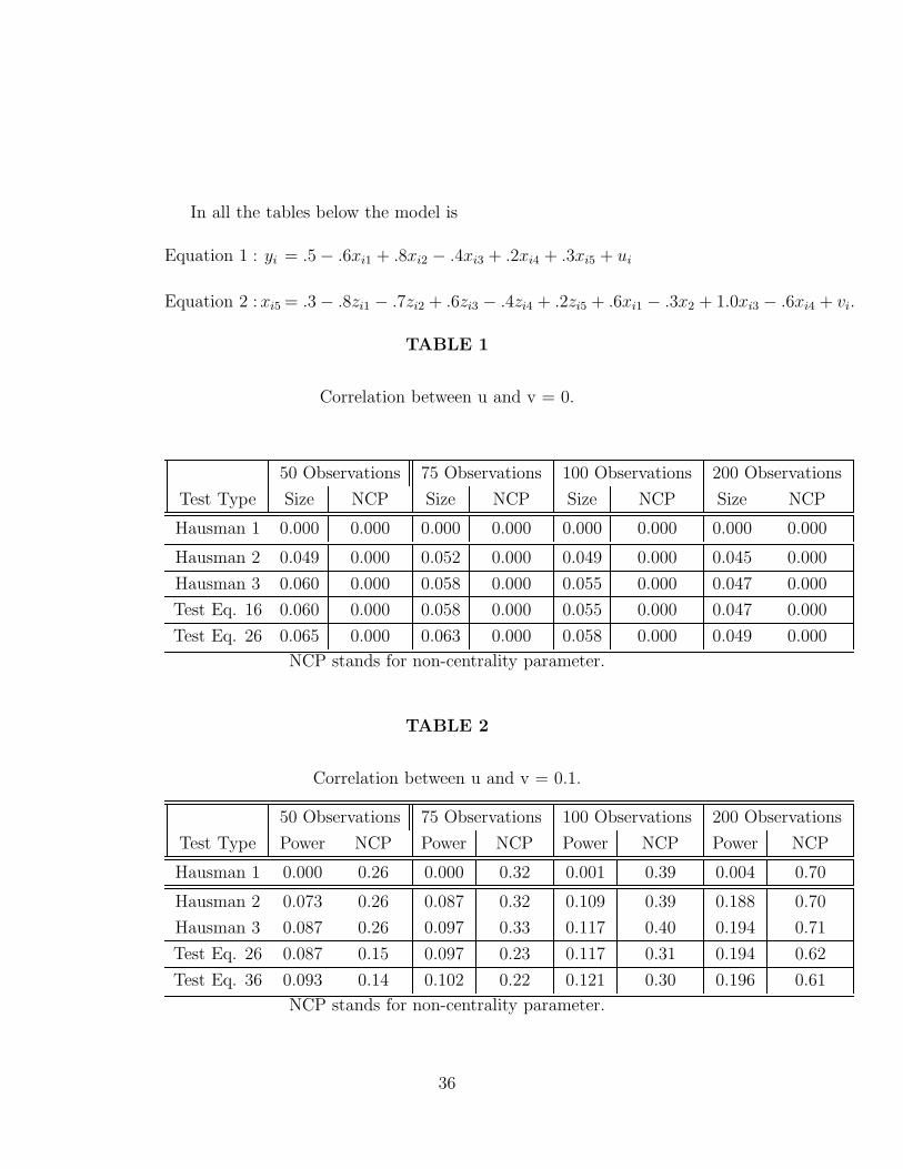
In all the tables below the model is
Equation 1 : yi = .5 − .6xi1 + .8xi2 − .4xi3 + .2xi4 + .3xi5 + ui
Equation 2 :xi5 = .3 − .8zi1 − .7zi2 + .6zi3 − .4zi4 + .2zi5 + .6xi1 − .3x2 + 1.0xi3 − .6xi4 + vi.
TABLE 1
Correlation between u and v = 0.
50 Observations 75 Observations 100 Observations 200 Observations
Test Type Size NCP Size NCP Size NCP Size NCP
Hausman 1 0.000 0.000 0.000 0.000 0.000 0.000 0.000 0.000
Hausman 2 0.049 0.000 0.052 0.000 0.049 0.000 0.045 0.000
Hausman 3 0.060 0.000 0.058 0.000 0.055 0.000 0.047 0.000
Test Eq. 16 0.060 0.000 0.058 0.000 0.055 0.000 0.047 0.000
Test Eq. 26 0.065 0.000 0.063 0.000 0.058 0.000 0.049 0.000
NCP stands for non-centrality parameter.
TABLE 2
Correlation between u and v = 0.1.
50 Observations 75 Observations 100 Observations 200 Observations
Test Type Power NCP Power NCP Power NCP Power NCP
Hausman 1 0.000 0.26 0.000 0.32 0.001 0.39 0.004 0.70
Hausman 2 0.073 0.26 0.087 0.32 0.109 0.39 0.188 0.70
Hausman 3 0.087 0.26 0.097 0.33 0.117 0.40 0.194 0.71
Test Eq. 26 0.087 0.15 0.097 0.23 0.117 0.31 0.194 0.62
Test Eq. 36 0.093 0.14 0.102 0.22 0.121 0.30 0.196 0.61
NCP stands for non-centrality parameter.
36

TABLE 3
Correlation between u and v = 0.3.
50 Observations 75 Observations 100 Observations 200 Observations
Test Type Power NCP Power NCP Power NCP Power NCP
Hausman 1 0.000 2.26 0.010 2.80 0.040 3.41 0.349 6.03
Hausman 2 0.307 2.26 0.488 2.80 0.626 3.41 0.916 6.03
Hausman 3 0.342 2.38 0.512 2.95 0.642 3.60 0.919 6.37
Test Eq. 26 0.342 1.36 0.512 2.07 0.642 2.78 0.919 5.60
Test Eq. 36 0.358 1.28 0.522 1.99 0.650 2.70 0.922 5.53
NCP stands for non-centrality parameter.
TABLE 4
Correlation between u and v = 0.5.
50 Observations 75 Observations 100 Observations 200 Observations
Test Type Power NCP Power NCP Power NCP Power NCP
Hausman 1 0.013 6.03 0.211 7.32 0.534 8.93 0.989 15.50
Hausman 2 0.764 6.03 0.931 7.32 0.982 8.93 1.000 15.50
Hausman 3 0.790 6.81 0.938 8.33 0.984 10.20 1.000 17.82
Test Eq. 26 0.790 3.78 0.938 5.75 0.984 7.71 1.000 15.58
Test Eq. 36 0.800 3.55 0.941 5.53 0.984 7.50 1.000 15.38
NCP stands for non-centrality parameter.
37

TABLE 5
Correlation between u and v = 0.7.
50 Observations 75 Observations 100 Observations 200 Observations
Test Type Power NCP Power NCP Power NCP Power NCP
Hausman 1 0.232 11.11 0.904 13.23 0.995 15.86 1.000 27.31
Hausman 2 0.989 11.11 1.000 13.23 1.000 15.86 1.000 27.31
Hausman 3 0.991 13.96 1.000 16.86 1.000 20.35 1.000 35.39
Test Eq. 26 0.991 7.42 1.000 11.26 1.000 15.12 1.000 30.51
Test Eq. 36 0.991 6.96 1.000 10.83 1.000 14.71 1.000 30.13
NCP stands for non-centrality parameter.
TABLE 6
Correlation between u and v = 0.9.
50 Observations 75 Observations 100 Observations 200 Observations
Test Type Power NCP Size NCP Power NCP Power NCP
Hausman 1 0.973 16.71 1.000 19.59 0.995 23.20 1.000 39.67
Hausman 2 1.000 16.71 1.000 19.59 1.000 23.20 1.000 39.67
Hausman 3 1.000 24.53 1.000 29.13 1.000 34.64 1.000 59.60
Test Eq. 26 1.000 12.25 1.000 18.63 1.000 25.00 1.000 50.43
Test Eq. 36 1.000 11.48 1.000 17.93 1.000 24.34 1.000 49.77
NCP stands for non-centrality parameter.
In Table 1 the first row lists only zeros; this is not because the actual
statistic is precisely zero, or the test did not function as anticipated; rather
it is zero because Hausman 1gets very few results “right”. Table 1 shows
that the Hausman 1, 2 tests do equally well but the test based on Eq. (36)
is slightly closer to the true size. In terms of the other tables that entail
correlated errors (u and v), Hausman 3 does generally better than Hausman
38

2, but the test based on Eq. (36), exhibits marginally higher power. As a
generalization, the power of all tests is rather low for a correlation of .1, but
it increases with the magnitude of the correlation, as well as the size of the
sample.
39


