Electronic copy available at: http://ssrn.com/abstract=1181367
1
Technical Analysis Around the World: Does it Ever Add Value?
Ben R. Marshall*, Rochester H. Cahan, Jared M. Cahan Massey University
New Zealand
Abstract
Technical analysis is not consistently profitable in the 49 countries that comprise the Morgan Stanley Capital Index once data snooping bias is accounted for. There is some evidence that technical trading rules perform better in emerging markets than developed markets, which is consistent with the finding of previous studies that these markets are less efficient, but this result is not strong. While we cannot rule out the possibility that technical analysis compliments other market timing techniques or that trading rules we do not test are profitable, we do show that over 5,000 trading rules do not add value beyond what may be expected by chance when used in isolation.
JEL Classification: G12, G14 Keywords: Technical Analysis, Quantitative, Market Timing
First Version: March 2008 This Version: August 2008
*Corresponding author. Department of Economics and Finance, College of Business, Massey University, Private Bag 11222, Palmerston North, New Zealand. Tel: +64 6 350 5799; Fax: +64 6 350 5651; E-Mail: [email protected].
Electronic copy available at: http://ssrn.com/abstract=1181367
2
Technical Analysis Around the World: Does it Ever Add Value?
Abstract
Technical analysis is not consistently profitable in the 49 countries that comprise the Morgan Stanley Capital Index once data snooping bias is accounted for. There is some evidence that technical trading rules perform better in emerging markets than developed markets, which is consistent with the finding of previous studies that these markets are less efficient, but this result is not strong. While we cannot rule out the possibility that technical analysis compliments other market timing techniques or that trading rules we do not test are profitable, we do show that over 5,000 trading rules do not add value beyond what may be expected by chance when used in isolation.
3
1. Introduction
Technical analysis, which involves making investment decisions based on past price
movements, continues to prove very popular with the investment community.1 Technical
trading rules are closely related to momentum trading strategies, which involve buying
(selling) winner (loser) stocks. Most academic authors find that momentum is an enduring
anomaly which has led to Fama and French (2008, p. 1) describing it as “pervasive.” These
two factors have resulted in a large amount of research energy being devoted to investigating
whether technical trading rules can add value. Most studies find that technical analysis does
not add value in the US equity market, but several authors have presented supportive evidence
in emerging markets.
We add to the literature by investigating the profitability of technical trading rules in
the 49 developed and emerging markets that make up the Morgan Stanley Capital Index
(MSCI). In doing so we propose that we make several important contributions. Firstly, we
consider in excess of 5,000 trading rules from four different rule families on each market.
Most previous studies consider a smaller number of rules (often less than 20).
Secondly, we apply a robust methodology which involves the application of two
alternative bootstrap techniques. The first was introduced by Brock, Lakonishok, and
LeBaron (1992) and the second was introduced by Sullivan, Timmermann, and White (1999).
These techniques have been shown to be more appropriate than the traditional t-test approach
which many authors in this area rely on. The Sullivan et al. (1999) technique is particularly
important as it enables us to control for data snooping bias, which they show can be the main
determinant of apparent technical analysis profits.
1 See Taylor and Allen (1992), Lui and Mole (1988), and Cheung and Chinn (2001) for surveys of investment professionals which illustrate the importance they ascribe to technical analysis.
4
Thirdly, our investigation of the same rules over a large number of markets enables
important comparisons to be made between developed and emerging markets. Chaudhuri and
Wu (2003) find that the random walk hypothesis can be rejected in many emerging markets
which implies that technical trading rules may be more profitable in these markets than they
are in developed markets. We are unaware of any previous studies that compare profits to the
same rules in both developed and emerging markets using data snooping adjusted bootstrap
techniques.
Finally, the careful design of our experiment ensures our results are likely to be of
interest to the investment community. The importance of international markets to portfolio
managers continues to increase with a recent survey finding the average allocation of money
to international markets by global funds was 57 percent in 2006 compared with just 37
percent in 2002.2 We purposely use MSCI indices as these are the benchmark adopted by
asset managers around the world. Portfolio managers could apply technical trading strategies
to time their entry into stocks within markets as part of a top-down investment approach as
outlined by Chan, Hameed, and Tong (2000), or they could use the trading rules we document
to time their purchase of the many ETFs and derivative products which are based on MSCI
indices. Olson (2004) shows that the profits to technical analysis have declined over time so
our focus on the recent period of 2001 – 2007, for which MSCI daily data are available, is
important. Finding profits on historical data may not necessarily imply that profits are
available today.
We find that many technical trading rules produce statistically significant profits
before consideration is given to data snooping bias, but this profitability disappears after data
snooping bias is taken into account. There is some evidence that technical analysis is more
profitable in emerging markets than it is in developed markets but this trend is relatively
2 http://www.iht.com/articles/2007/04/25/bloomberg/bxfund.php.
5
weak. We conclude that the technical trading rules we consider do not add value beyond what
might be expected by chance as a stand-alone market timing tool, but we cannot rule out the
possibility that these technical trading rules can compliment some other investment technique,
or that other trading rules are profitable.3 Our intention was to also assess the economic
significance of the most profitable trading rules, but given that the profitability of even the
best performing rule on each market does not fall outside that which can be explained by data
snooping we do not proceed with this step.
The rest of this paper is organized as follows: Section 2 contains a brief review of
the literature. Our data and methodology are outlined in Section 3. We present our results in
Section 4 and discuss our conclusions in Section 5.
2. Literature Review
The majority of US studies find that technical analysis does not add value after
transaction costs are accounted for. In a seminal paper, Brock, Lakonishok and LeBaron
(hereafter BLL) (1992) test Variable Moving Average (VMA), Fixed Moving Average
(FMA) and Trading Rang Breakout (TRB) rules on the Dow Jones Industrial Average and
find that statistically significant profits are generated. However, Bessembinder and Chan
(1998) show that these profits do not exceed reasonable estimates of transaction costs. Allen
and Karjalainen (1999) reach a similar conclusion after applying trading rules selected by
genetic algorithms to the US equity market. While there are gross profits available, the
profitability is removed once transaction costs are accounted for. Exceptions to the above are
the minority but they do exist. For instance Cooper (1999) finds filter rules based on both
3 There are a huge number of different trading rules used by practitioners and many systems include customized parameter specifications and combinations of different rules but we limit our analysis to those most commonly studied in the literature, as summarized by Sullivan et al (1999). We provide detailed explanations of these rules in Section 3.
6
price and volume generate profits after relatively low estimates of transaction costs are taken
into account.
Authors who have tested trading rules on developed markets outside the US
generally also find that the profits generated do not offset transactions costs. Hudson,
Dempsey, and Keasey (1996) apply the BLL (1992) trading rules in the UK equity market and
find that they generate profitable signals but these profits are not large enough to offset
transaction costs. Precise estimation of the costs incurred in exploiting technical analysis are
often difficult to estimate but Bessembinder and Chan (1995) find BLL (1992) trading rules
are less profitable in the developed markets of Hong Kong and Japan than they are in
emerging markets.
The evidence of profitability over and above transactions costs appears to be the
most compelling in emerging markets. Parisi and Vasquez (2000) document large profits to
the BLL (1992) trading rules in the Chilean stock market. They do not consider transactions
costs, however, several other authors do. Bessembinder and Chan (1995) find BLL (1992)
trading rules produce profits in excess of transaction costs in the emerging markets of
Malaysia, Thailand, and Taiwan. Ito (1999) also tests BLL (1992) trading rules and finds
profitability beyond transaction costs in Indonesian, Mexican and Taiwanese equity indices.
Finally, Ratner and Leal (1999) test 10 VMA rules on the emerging markets of India, Korea,
Malaysia, Philippines, Taiwan, Thailand, Argentina, Brazil, Chile, and Mexico. They find
some evidence of profitability in most markets after transactions costs but most of this is
centred in the markets of Mexico, Philippines, Taiwan, and Thailand.
It is important to note that none of the studies discussed above formally address the
issue of data snooping bias with the technique outlined by Sullivan, Timmermann, and White
(1999). Drawing on the work of White (2000), these authors suggest that rules that are the
most profitable are the very rules that are the most likely to be examined over time. This
7
means that it is important to consider the profitability of any rule in the context of the full
universe of rules from which it was drawn. We apply the technique advocated by Sullivan,
Timmermann, and White (1999) to our test of technical analysis profitability in both
developed and emerging markets.
3. Data, Trading Rule Specifications, and Methodology
3.1. Data
We source data for the 23 developed markets and 26 emerging markets that
comprise the MSCI from Datastream. We report results for their total return series in US$ but
we test local currency series for a number of countries and verify there results are
qualitatively identical. We source data for the 1/1/2001 – 31/12/2007 period for each country
with the exception of Greece whose data begins at 1/6/2001. These periods correspond to the
first date that daily data is available for the MSCI for each country. We suggest that the focus
on data for a recent time period is appropriate as Olson (2004) has shown that the returns to
technical analysis have declined over time, which means that documenting profits on more
historical series may not be relevant.
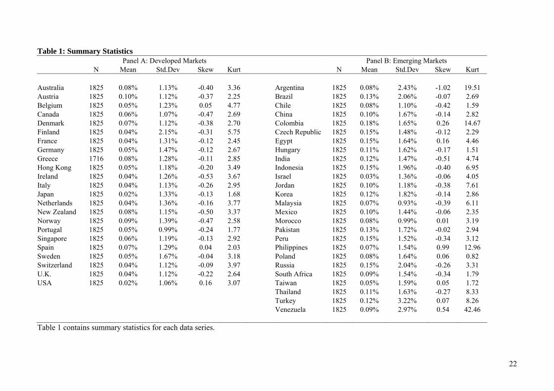
The summary statistics presented in Table 1 illustrate that emerging markets have,
on average, out-performed their developed market counterparts over the period of our study
(mean daily return of 0.11% for emerging markets versus 0.05% for developed markets), but
they also involve higher risks. The average standard deviation across the emerging markets is
1.70% versus an average of 1.27% for developed markets. All the markets we study have
gained over the 2001-2007 period. Columbia is the best performing while the USA is the
8
worst performing. Turkey is the most risky market, based on standard deviations, while
Malaysia is the least risky. Many markets display skewness and kurtosis which reinforces the
appropriateness of our non-parametric bootstrap methodologies, which we discuss in detail in
Section 3.3.
[Insert Table 1 About Here]
3.2. Trading Rule Specifications
We apply 5,806 of the technical trading rules suggested by Sullivan, Timmermann,
and White (here after STW) (1999). STW (1999) test in excess of 7,000 rules, but one of
their five rule families requires volume data which are not available for the MSCI indices we
examine. The four rule families we test are Filter Rules, Moving Average Rules, Support and
Resistance Rules, and Channel Break-outs. STW (1999) provide an excellent description of
each rule in the appendix of their paper, which we recommend to the interested reader.
Basic Filter Rules involve opening long (short) positions after price increases
(decreases) by x% and closing these postions when price decreases (increases) by x% from a
subsequent high (low). We test these rules and two variations. Following STW (1999) we also
investigate defining subsequent high (lows) as the highest (lowest) closing price achieved
while holding a particular long (short) position, and a most recent closing price that is less
(greater) than the e previous closing prices. We also apply rules that permit a neutral position.
These involve closing a long (short) position when price decreases (increases) y percent from
the previous high (low). Finally, we also consider rules that involve holding a position for a
pre-specified number of periods, c, thereby ignoring other signals generated during this time.
9
Moving Average rules generate buy (sell) signals when the price or a short moving
average moves above (below) a long moving average. We follow STW (1999) and apply two
filters. The first variation involves the requirement that the shorter moving average exceeds
the longer moving average by a fixed amount, b. The second variation involves the
requirement that a signal, either buy or sell, remains valid for a prespecified number of
periods, d, before the signal is acted upon. A final variation we consider is holding a position
for a prespecified number of periods, c.
Our third rule family, Support and Resistance or “Trading Range Break” rules
involve opening a long (short) position when the closing price breaches the maximum
(minimum) price over the previous n periods. A variation we consider involves using the most
recent closing price that is greater (less) than the e previous closing price as the extreme price
level that triggers an entry or exit signal. Consistent with the other rule families, positions can
be held for fixed number of periods, c. Finally, we follow STW (1999) and impose a fixed
percentage band filter, b, and a time delay filter, d.
Our final family of rules is Channel Breakouts. In accordance with STW (1999), the
Channel Breakout rules we test involve opening long (short) positions when the closing price
moves above (below) the channel. A channel is defined as a situation when the high over the
previous n periods is within x percent of the low over the previous n periods. Positions are
held for a fixed number of periods, c. A version of Channel Breakout rules which involve a
fixed band, b, being applied to the channel as a filter is also investigated.
3.3. Methodology
We follow the approach of Marshall, Cahan, and Cahan (2008a, b) and apply both
the BLL (1992) and STW (1999) bootstrap methodologies. The BLL (1992) methodology
10
involves fitting a null model to the data and estimating its parameters. The residuals are then
randomly re-sampled 500 times and used, together with the models parameters, to generate
random price series which exhibit the same characteristics as the original series. BLL (1992)
find that results do not differ in any important way regardless of which null model is used,
however, we follow (Kwon and Kish (2002) and Marshall, Cahan, and Cahan (2008b) and use
the GARCH-M null model which we present in equations 1 to 3 (see BLL, 1992 for a detailed
description of this model):
rt = α + γσt2 + βεt-1 + εt (1)
σt2 = α0 + α1εt-1
2 + βσt-12 (2)
εt = σt zt zt ~ N(0,1) (3)
The basic premise behind the BLL (1992) bootstrap methodology is that in order for
a trading rule to be statistically significant at the α level it must produce larger profits on less
than α% of the bootstrapped series than on the original series. In accordance with BLL (1992)
we define the buy (sell) return as the mean return for each day the rule is long (short). The
difference between the two means is the buy-sell return and the proportion of times the buy-
sell profit for the rule is greater on the 500 random series than the original series is the buy-
sell p-value.
The second bootstrap test we apply is from STW (1999). Their test is based on the
techniques introduced by White (2000), which are based on the premise that the statistical
significance of any profits to a technical trading rule need to be adjusted to account for the
fact that the trading rule in question was drawn from a universe of trading rules. This means
that it is possible that its profitability is simply due to chance. In this sense the STW (1999)
approach is different from the BLL (1992) technique which evaluates each rule in isolation.
11
In accordance with STW (1999), we define ),...,1(, Mkf tk = as the period t return
generated by the k-th trading rule relative to the benchmark index return at time t). The main
statistic we are interested in is the mean period relative return from the k-th rule,
∑ ==
T
t tkk Tff1 , / , where T is the number of days in the sample.
Consistent with STW (1999), we use the null hypothesis that the performance of the
best trading rule on each index is no better than the benchmark performance, i.e.,
0max:,...,10 ≤
= kMkfH
Following STW (1999) we use a stationary bootstrap of on the M values of kf to
test the null hypothesis.4 This involves re-sampling with replacement the time-series of
relative returns B times for each of the M rules. For each of the M rules, the same B
bootstrapped time-series are used. In accordance with STW (1999), we set B = 500. For the k-
th rule, this results in B means being generated, which we denote ),...,1(, Bbf bk =∗ , from the B
re-sampled time-series, where:
),...,1(,/1
*,,, BbTff
T
tbtkbk ==∑
=
∗ .
The test two statistics employed in the test are:
][max,...,1 kMkM fTV
==
and
).,...,1(,)]([max *,,...,1
*, BbffTV kbkMkbM =−=
=
4 The interested reader should consult Appendix C of STW (1999) for more details.
(4)
(5)
(6)
(7)
12
The test statistic is derived by comparing MV to the quantiles of the
*,bMV distribution. In other words, we compare the maximum mean relative return from the
original series, to that from each of the 500 bootstraps. Or, put another way, the test evaluates
the performance of the best rule with reference to the performance of the whole universe and
takes account of data snooping bias in the process.
4. Results
Our results indicate that there is no evidence that the technical trading rules we
consider consistently add value after data snooping bias is taken into account. There is
widespread evidence of rules producing statistically significant profits, but the statistical
significance is not strong enough to rule out the possibility that it could be due to chance. We
find some evidence that technical analysis is more profitable in emerging markets but this is
relatively weak. We intended to also determine the economic significance of the most
profitable trading rules, but given that the profitability of even the best performing rule on
each market is not sufficient to rule out a data snooping explanation we see little point
proceeding with this analysis.
The first part of the results we present are generated using the bootstrapping
technique of BLL (1992). This involves fitting a null model to the data, in our case GARCH-
M, and bootstrapping the residuals to generate random series with the same time-series
characteristics as the original series. A trading rule is then run over the random series and the
profits compared to those generated on the original series. For a rule to be statistically
significant at the 5% level the profits must be larger on the random bootstrapped series than
the original series less than 5% of the time. The BLL (1992) approach takes no account of
13
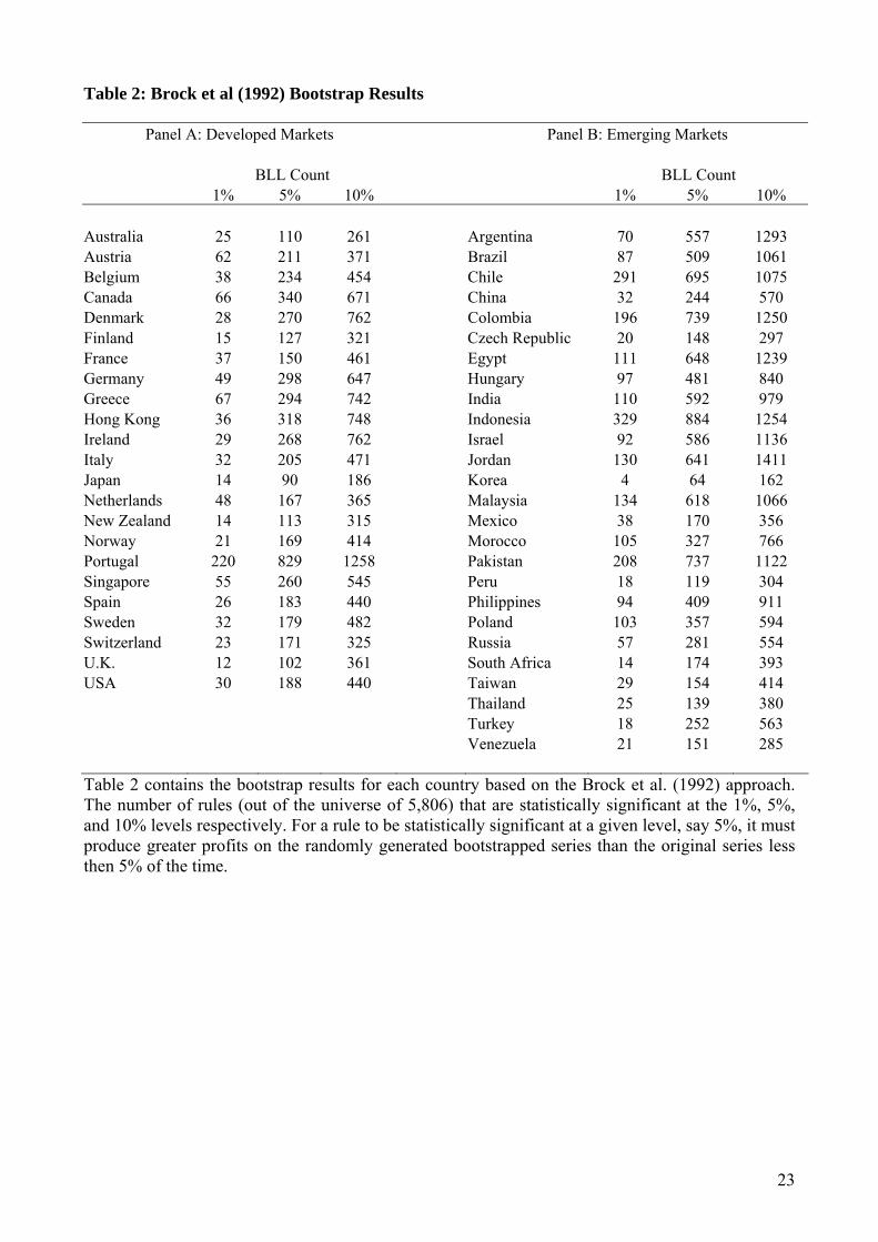
data snooping bias. In Table 2 we present the number of rules, out of the total universe of
5,806, which are profitable at the 1%, 5%, and 10% levels respectively. Results for developed
(emerging) markets are presented in Panel A (Panel B).
The Table 2 results indicate that technical analysis appears to be more profitable on
emerging markets than developed markets. Across all emerging markets the average number
of rules that are statistically significant at the 1%, 5%, and 10% level is 90, 395, and 791
respectively. This equivalent average numbers of profitable rules for developed markets are
41, 220, and 492. Comparing the developed and emerging markets another way, we see that
15 out of the 26 developed markets have more than 10% of the total number of rules (i.e.
more than 580) statistically significant at the 10% level compared to 7 of the 23 developed
markets.
Turning to the individual results, it is clear that there is a lot of variation in the
number of rules that are statistically significant in the developed and emerging market sub-
samples. Of the developed markets, Japan has the fewest statistically significant rules (186 at
the 10% level), while Portugal has the most (1258 at the 10% level). Within the emerging
markets, Korea has the fewest number of statistically significant rules at the 10% level (162)
while Indonesia has the most (1254).
[Insert Table 2 About Here]
We now consider the results generated by the STW (1999) bootstrap techniques.
Unlike, the BLL (1992) results, data-snooping bias is accounted for in these results. We
present the nominal p-value which is generated by the best performing rule before data
snooping bias is accounted for. It is important to note that the bootstrapping technique used by
STW (1999) to generate the nominal p-value is different to the BLL (1992) procedure. The
14
STW p-value includes the adjustment for data snooping bias. We also present the following
statistics for the best performing rule: the average daily return, the average return per trade,
the total number of trades, the number of winning trades, the number of losing trades, and the
average number of days per trade.
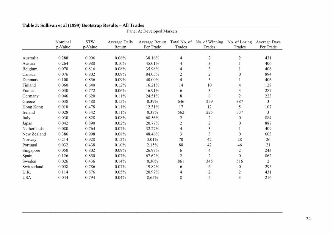
The developed market results in Panel A of Table 3 indicate that the best trading rule
produces profits that are statistically significant at the 10% level or better, based on the STW
(1999) bootstrap procedure, in 16 of the 23 developed markets prior to any adjustment for
data snooping bias. As noted earlier, this bootstrap procedure is different to that developed by
BLL (1992). This accounts for the fact that some markets have no rules that generate profits
that are statistically significant in these results whereas each market has rules that generate
statistically significant profits based on the BLL (1992) technique. While there may be some
differences between the results generated by the BLL (1992) and STW (1999) techniques
prior to data snooping bias adjustment, the result after this adjustment has been made is
unambiguously clear. None of the developed markets have a trading rule that produces
statistically significant profits after data snooping bias is accounted for. Data snooping is
clearly a major issue, judging by the differences between the nominal and STW p-values. For
instance in the case of Singapore the nominal p-value is 0.05, yet when data snooping bias is
taken into account the p-value increases to 0.802.
It is clear that there is a large amount of variation in the trading frequency of the best
performing trading rule across the different markets. In markets such as Australia and Austria
the most profitable rule is from the Support and Resistance rule family. In both cases the rule
only signals a total of 4 trades in the entire seven year period. The average number of days a
trade is open is 431 in the case of Australia. This explains why the average return per trade is
very sizable (38.16%) yet the average daily return is just 0.08%, and therefore almost
15
identical to the unconditional average daily return (0.08%) in the Australian market during the
period we study.
At the other end of the spectrum, the best performing rule in other markets signals
many trades. In Sweden the optimal rule is a short term moving average rule which generates
a total of 861 trading signals resulting in an average holding period of just 2 days. The results
for this rule illustrate that a technical trading rule can be profitable overall even if it generates
more losing than winning trades. The best performing rule in Sweden only signals a winning
trade 40% of the time but it is still profitable overall due to the fact that the average profits
generated by its winning trades outweigh the average profits generated by its losing trades.
[Insert Table 3 About Here]
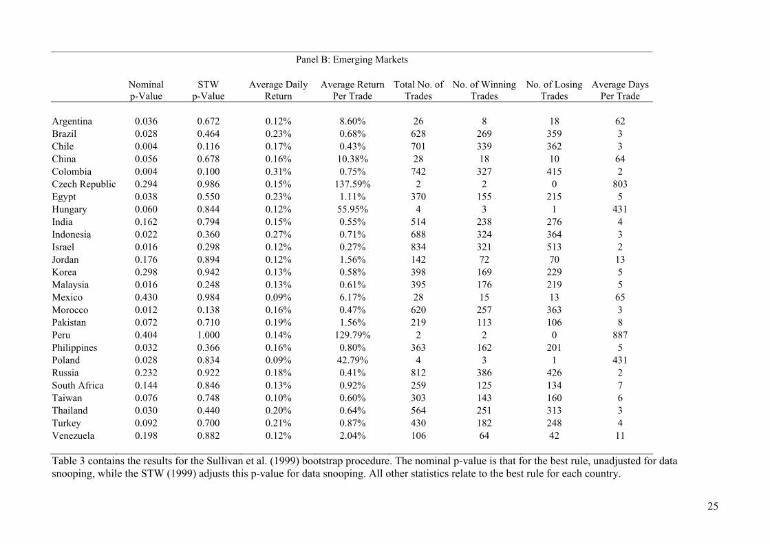
The emerging market results in Panel B of Table 3 are similar to their developed
market counterparts in that no market has a trading rule that generates profits that are
statistically significant at the 10% level after data snooping bias is taken into account. The
closest any market gets is Colombia, whose best performing rule only just fails to be
statistically significant after data snooping bias adjustment (p-value = 0.1001). One clear
difference between the best rule on developed and emerging markets is the number of trading
signals generated by the rule. In developed markets the most profitable rule is more often than
not one that generates few trading signals, and often comes from the Support and Resistance
rule family. The opposite is the case in emerging markets. With a few exceptions, the most
profitable rule in emerging markets is one that generated numerous trading signals (often in
excess of 300) over the seven year sample period we consider. The most profitable rules in
emerging markets are often short-term trading rule from the Moving Average or Filter Rule
family.
16
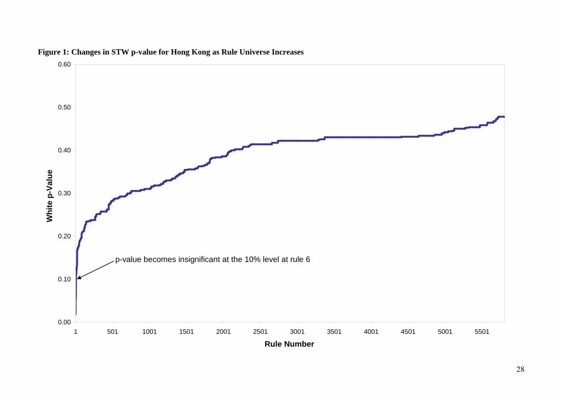
The data snooping adjustment advocated by STW (1999) that we employ in this
paper involves adjusting the statistical significance of the most profitable trading rule to
account for the universe of rules from which it is selected. As the size of the universe
increases, the STW (1999) data snooping adjusted p-value declines. We investigate whether
we are unfairly penalizing the best performing trading rule in each market by comparing it to
a large number of unprofitable rules. We proceed as follows: Firstly, we select the best
performing trading rule for a market from all 5,806 rules run. We then calculate the STW
(1999) p-value based on that rule being the only one in the universe, based on there being two
rules in the universe, based on there being three rules in the universe and so on up to a rule
universe of 5,806. We add the most profitable rules first so as to give the best performing rule
the most chance of remaining profitable as the rule universe increases.
We display the results of this analysis for Hong Kong in Figure 1. We choose Hong
Kong because the best performing rule in this market has the lowest nominal p-value out of
the best performing rules in all developed markets. In other words, the most profitable rule in
Hong Kong goes from being highly statistically significant prior to any adjustment for data
snooping (p-value = 0.018) to highly insignificant after the entire rule universe is included in
the data snooping adjustment procedure (p-value = 0.478). Figure 1 reveals that the best
performing trading rule in Hong Kong becomes insignificant at the 10% level after just 6
rules are added to the rule universe. This indicates that data snooping bias is a big issue in our
tests. In other words, the best performing rule is not losing its statistically significance after
adjustment for data snooping bias simply because a large universe of rules is being included
in the data snooping test.
[Insert Figure 1 About Here]

17
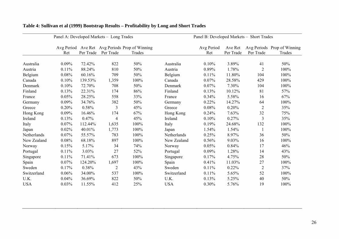
Each technical trading rule generates both long and short signals so we conclude by
investigating the possibility that the performance of technical trading rules is not uniform
across the long and short signals they generate. The results, including the average period
return, the average return per trade, the average number of periods per trade, and the
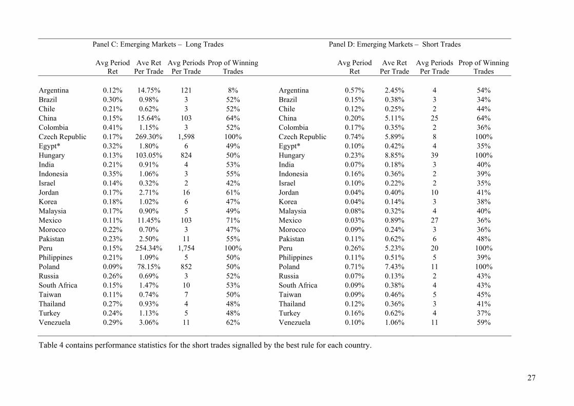
proportion of trades that are winning trades, are presented in Table 4. Short trades seem to be
more profitable than long trades in developed markets, with the average period return being
higher for short trades in 15 of the 23 developed countries. It is also clear that long trades tend
to spend a lot longer in the market on average in developed countries.
The emerging market results presented in Panel B indicate long trades tend to be
more profitable than short trades in emerging markets. The average period return is larger
long trades in 20 of the 26 markets. There is also the trend of long trades spending more time
in the market, although this result is not as strong as it was in developed markets.
[Insert Table 4 About Here]
In summary, we conclude that there is some evidence that long trades are more
profitable in emerging markets and short trades are more profitable in developed market based
on the optimal trading rule in each market. However, it must be remembered that the optimal
trading rule in each market does not produce profits that are statistically significant beyond
that which might be expected by chance given the possibility of data snooping.
5. Conclusions
We investigate the profitability of technical trading rules in the 49 developed and
emerging markets that comprise the Morgan Stanley Capital Index (MSCI). In do so we

18
suggest that we make several contributions. We consider in excess of 5,000 trading rules
using two alternative bootstrapping techniques, with one of these allowing us to take account
of possible data snooping bias. To the best of our knowledge, we are the first to consider the
same vast universe of trading rules using the most robust methodologies in such a wide range
of developed and emerging markets. This enables us to make important comparisons of
profitability across markets.
We find no evidence that the profits to the technical trading rules we consider are
greater than those that might be expected due to random data variation, once we take account
of data snooping bias. There is some evidence that technical analysis works better in
emerging markets, which is consistent with the literature that documents that these markets
are less efficient, but this is not a strong result.
We suggest that our results imply that simple technical trading rules do not
consistently add value when applied to a broad range of international markets. We cannot rule
out the possibility that technical analysis can be used to compliment other investment
techniques, or that trading rules other than the ones we examine are profitable. However, we
can say that over 5,000 popular technical trading rules do not appear to add value, beyond that
which may be explained by chance, when used in isolation.
19
References
Allen, F., Karjalainen, R., 1999. Using genetic algorithms to find technical trading rules.
Journal of Financial Economics 51, 245-271.
Bessembinder, H., Chan, K., 1995. The profitability of technical trading rules in the Asian
stock markets. Pacific-Basin Finance Journal 3, 257-284.
Bessembinder, H., Chan, K., 1998. Market efficiency and the returns to technical analysis.
Financial Management 27(2), 5-13.
Brock, W., Lakonishok, J., LeBaron, B., 1992. Simple technical trading rules and the
stochastic properties of stock returns. Journal of Finance 48(5), 1731-1764.
Chan, K., Hameed, A., Tong, W., 2000. Profitability of Momentum Strategies in the
International Equity Markets, Journal of Financial and Quantitative Analysis 35(2), 153-172.
Chaudhuri, K., Wu, Y., 2003. Random walk versus breaking trend in stock prices: Evidence
from emerging markets. Journal of Banking and Finance 27, 575–592.
Cheung, Y.W., Chinn, M.D., 2001. Currency traders and exchange rate dynamics: a survey of
the US market. Journal of International Money and Finance 20(4), 439-471
Cooper, M., 1999. Filter rules based on price and volume in individual security overreaction.
Review of Financial Studies 12(4), 901-935.
20
Fama, E., French, K. 2008. Dissecting anomalies. Journal of Finance – forthcoming.
Hudson, R., Dempsey, M., Keasey, K., 1996. A note on weak form efficiency of capital
markets: The application of simple technical trading rules to UK prices 1935-1994. Journal of
Banking and Finance 20, 1121-1132.
Ito, A., 1999. Profits on Technical Trading Rules and Time-Varying Expected Returns:
Evidence from Pacific-Basin Equity Markets, Pacific-Basin Finance Journal 7(3-4), 283-330.
Kwon, K-Y, Kish, R., 2002. A Comparative Study of Technical Trading Strategies and
Return Predictability: An Extension of Brock, Lakonishok, and LeBaron (1992) Using NYSE
and NASDAQ Indices, Quarterly Review of Economics and Finance 42(3), 611-631.
Lui, Y., Mole, D., 1998. The use of fundamental and technical analysis by foreign exchange
dealers: Hong Kong evidence. Journal of International Money and Finance 17, 535-545.
Marshall, B.R, Cahan, R.H., Cahan, J.M., 2008a. Does Intraday Technical Analysis in the
U.S. Equity Market Have Value? Journal of Empirical Finance 15, 199-210.
Marshall, B.R, Cahan, R.H., Cahan, J.M., 2008b. Can Commodity Futures Be Profitably
Traded with Quantitative Market Timing Strategies? Journal of Banking and Finance –
Forthcoming
Olson, D., 2004. Have trading rule profits in the currency markets declined over time? Journal
of Banking and Finance 28, 85-105.
21
Parisi, F., Vasquez, A., 2000. Simple technical trading rules of stock returns: evidence from
1987 to 1998 in Chile. Emerging Markets Review 1, 152-164.
Ratner, M., Leal, R., 1999. Tests of Technical Trading Strategies in the Emerging Equity
Markets of Latin America and Asia, Journal of Banking and Finance 23(12), 1887-1905.
Sullivan, R., Timmermann, A., White, H., 1999. Data-snooping, technical trading rule
performance, and the bootstrap. Journal of Finance 24(5), 1647-1691.
Taylor, M., Allen, H., 1992. The use of technical analysis in the foreign exchange market.
Journal of International Money and Finance 11(3), 301-314.
White, H., 2000. A Reality Check for data snooping. Economterica 68 (5), 1097–1126.
22
Table 1: Summary Statistics Panel A: Developed Markets Panel B: Emerging Markets
N Mean Std.Dev Skew Kurt N Mean Std.Dev Skew Kurt Australia 1825 0.08% 1.13% -0.40 3.36 Argentina 1825 0.08% 2.43% -1.02 19.51 Austria 1825 0.10% 1.12% -0.37 2.25 Brazil 1825 0.13% 2.06% -0.07 2.69 Belgium 1825 0.05% 1.23% 0.05 4.77 Chile 1825 0.08% 1.10% -0.42 1.59 Canada 1825 0.06% 1.07% -0.47 2.69 China 1825 0.10% 1.67% -0.14 2.82 Denmark 1825 0.07% 1.12% -0.38 2.70 Colombia 1825 0.18% 1.65% 0.26 14.67 Finland 1825 0.04% 2.15% -0.31 5.75 Czech Republic 1825 0.15% 1.48% -0.12 2.29 France 1825 0.04% 1.31% -0.12 2.45 Egypt 1825 0.15% 1.64% 0.16 4.46 Germany 1825 0.05% 1.47% -0.12 2.67 Hungary 1825 0.11% 1.62% -0.17 1.51 Greece 1716 0.08% 1.28% -0.11 2.85 India 1825 0.12% 1.47% -0.51 4.74 Hong Kong 1825 0.05% 1.18% -0.20 3.49 Indonesia 1825 0.15% 1.96% -0.40 6.95 Ireland 1825 0.04% 1.26% -0.53 3.67 Israel 1825 0.03% 1.36% -0.06 4.05 Italy 1825 0.04% 1.13% -0.26 2.95 Jordan 1825 0.10% 1.18% -0.38 7.61 Japan 1825 0.02% 1.33% -0.13 1.68 Korea 1825 0.12% 1.82% -0.14 2.86 Netherlands 1825 0.04% 1.36% -0.16 3.77 Malaysia 1825 0.07% 0.93% -0.39 6.11 New Zealand 1825 0.08% 1.15% -0.50 3.37 Mexico 1825 0.10% 1.44% -0.06 2.35 Norway 1825 0.09% 1.39% -0.47 2.58 Morocco 1825 0.08% 0.99% 0.01 3.19 Portugal 1825 0.05% 0.99% -0.24 1.77 Pakistan 1825 0.13% 1.72% -0.02 2.94 Singapore 1825 0.06% 1.19% -0.13 2.92 Peru 1825 0.15% 1.52% -0.34 3.12 Spain 1825 0.07% 1.29% 0.04 2.03 Philippines 1825 0.07% 1.54% 0.99 12.96 Sweden 1825 0.05% 1.67% -0.04 3.18 Poland 1825 0.08% 1.64% 0.06 0.82 Switzerland 1825 0.04% 1.12% -0.09 3.97 Russia 1825 0.15% 2.04% -0.26 3.31 U.K. 1825 0.04% 1.12% -0.22 2.64 South Africa 1825 0.09% 1.54% -0.34 1.79 USA 1825 0.02% 1.06% 0.16 3.07 Taiwan 1825 0.05% 1.59% 0.05 1.72 Thailand 1825 0.11% 1.63% -0.27 8.33 Turkey 1825 0.12% 3.22% 0.07 8.26 Venezuela 1825 0.09% 2.97% 0.54 42.46 Table 1 contains summary statistics for each data series.
23
Table 2: Brock et al (1992) Bootstrap Results
Table 2 contains the bootstrap results for each country based on the Brock et al. (1992) approach. The number of rules (out of the universe of 5,806) that are statistically significant at the 1%, 5%, and 10% levels respectively. For a rule to be statistically significant at a given level, say 5%, it must produce greater profits on the randomly generated bootstrapped series than the original series less then 5% of the time.
Panel A: Developed Markets Panel B: Emerging Markets BLL Count BLL Count 1% 5% 10% 1% 5% 10% Australia 25 110 261 Argentina 70 557 1293 Austria 62 211 371 Brazil 87 509 1061 Belgium 38 234 454 Chile 291 695 1075 Canada 66 340 671 China 32 244 570 Denmark 28 270 762 Colombia 196 739 1250 Finland 15 127 321 Czech Republic 20 148 297 France 37 150 461 Egypt 111 648 1239 Germany 49 298 647 Hungary 97 481 840 Greece 67 294 742 India 110 592 979 Hong Kong 36 318 748 Indonesia 329 884 1254 Ireland 29 268 762 Israel 92 586 1136 Italy 32 205 471 Jordan 130 641 1411 Japan 14 90 186 Korea 4 64 162 Netherlands 48 167 365 Malaysia 134 618 1066 New Zealand 14 113 315 Mexico 38 170 356 Norway 21 169 414 Morocco 105 327 766 Portugal 220 829 1258 Pakistan 208 737 1122 Singapore 55 260 545 Peru 18 119 304 Spain 26 183 440 Philippines 94 409 911 Sweden 32 179 482 Poland 103 357 594 Switzerland 23 171 325 Russia 57 281 554 U.K. 12 102 361 South Africa 14 174 393 USA 30 188 440 Taiwan 29 154 414 Thailand 25 139 380 Turkey 18 252 563 Venezuela 21 151 285
24
Table 3: Sullivan et al (1999) Bootstrap Results – All Trades Panel A: Developed Markets
Nominal p-Value
STW p-Value
Average Daily Return
Average Return Per Trade
Total No. of Trades
No. of Winning Trades
No. of Losing Trades
Average Days Per Trade
Australia 0.288 0.996 0.08% 38.16% 4 2 2 431 Austria 0.264 0.988 0.10% 45.01% 4 3 1 406 Belgium 0.070 0.816 0.08% 35.98% 4 3 1 406 Canada 0.076 0.802 0.09% 84.05% 2 2 0 894 Denmark 0.100 0.856 0.09% 40.00% 4 3 1 406 Finland 0.060 0.640 0.12% 16.21% 14 10 4 128 France 0.030 0.772 0.06% 16.91% 6 3 3 287 Germany 0.046 0.620 0.11% 24.51% 8 6 2 223 Greece 0.038 0.488 0.15% 0.39% 646 259 387 3 Hong Kong 0.018 0.478 0.11% 12.31% 17 12 5 107 Ireland 0.028 0.342 0.11% 0.37% 562 225 337 3 Italy 0.030 0.828 0.08% 68.56% 2 2 0 884 Japan 0.042 0.890 0.02% 20.77% 2 2 0 887 Netherlands 0.080 0.764 0.07% 32.27% 4 3 1 409 New Zealand 0.386 0.998 0.08% 48.46% 3 3 0 603 Norway 0.214 0.928 0.12% 3.01% 70 42 28 26 Portugal 0.032 0.438 0.10% 2.15% 88 42 46 21 Singapore 0.050 0.802 0.09% 26.97% 6 4 2 243 Spain 0.126 0.850 0.07% 67.62% 2 2 0 862 Sweden 0.026 0.436 0.14% 0.30% 861 345 516 2 Switzerland 0.058 0.786 0.07% 19.82% 6 6 0 295 U.K. 0.114 0.876 0.05% 20.97% 4 2 2 431 USA 0.044 0.794 0.04% 8.65% 8 5 3 216
25
Panel B: Emerging Markets
Nominal p-Value
STW p-Value
Average Daily Return
Average Return Per Trade
Total No. of Trades
No. of Winning Trades
No. of Losing Trades
Average Days Per Trade
Argentina 0.036 0.672 0.12% 8.60% 26 8 18 62 Brazil 0.028 0.464 0.23% 0.68% 628 269 359 3 Chile 0.004 0.116 0.17% 0.43% 701 339 362 3 China 0.056 0.678 0.16% 10.38% 28 18 10 64 Colombia 0.004 0.100 0.31% 0.75% 742 327 415 2 Czech Republic 0.294 0.986 0.15% 137.59% 2 2 0 803 Egypt 0.038 0.550 0.23% 1.11% 370 155 215 5 Hungary 0.060 0.844 0.12% 55.95% 4 3 1 431 India 0.162 0.794 0.15% 0.55% 514 238 276 4 Indonesia 0.022 0.360 0.27% 0.71% 688 324 364 3 Israel 0.016 0.298 0.12% 0.27% 834 321 513 2 Jordan 0.176 0.894 0.12% 1.56% 142 72 70 13 Korea 0.298 0.942 0.13% 0.58% 398 169 229 5 Malaysia 0.016 0.248 0.13% 0.61% 395 176 219 5 Mexico 0.430 0.984 0.09% 6.17% 28 15 13 65 Morocco 0.012 0.138 0.16% 0.47% 620 257 363 3 Pakistan 0.072 0.710 0.19% 1.56% 219 113 106 8 Peru 0.404 1.000 0.14% 129.79% 2 2 0 887 Philippines 0.032 0.366 0.16% 0.80% 363 162 201 5 Poland 0.028 0.834 0.09% 42.79% 4 3 1 431 Russia 0.232 0.922 0.18% 0.41% 812 386 426 2 South Africa 0.144 0.846 0.13% 0.92% 259 125 134 7 Taiwan 0.076 0.748 0.10% 0.60% 303 143 160 6 Thailand 0.030 0.440 0.20% 0.64% 564 251 313 3 Turkey 0.092 0.700 0.21% 0.87% 430 182 248 4 Venezuela 0.198 0.882 0.12% 2.04% 106 64 42 11 Table 3 contains the results for the Sullivan et al. (1999) bootstrap procedure. The nominal p-value is that for the best rule, unadjusted for data snooping, while the STW (1999) adjusts this p-value for data snooping. All other statistics relate to the best rule for each country.
26
Table 4: Sullivan et al (1999) Bootstrap Results – Profitability by Long and Short Trades Table 4 contains performance statistics for the long trades signalled by the best rule for each country.
Panel A: Developed Markets – Long Trades Panel B: Developed Markets – Short Trades
Avg Period
Ret Ave Ret
Per Trade Avg Periods
Per Trade Prop of Winning
Trades Avg Period
Ret Ave Ret
Per Trade Avg Periods
Per Trade Prop of Winning
Trades Australia 0.09% 72.42% 822 50% Australia 0.10% 3.89% 41 50% Austria 0.11% 88.24% 810 50% Austria 0.89% 1.78% 2 100% Belgium 0.08% 60.16% 709 50% Belgium 0.11% 11.80% 104 100% Canada 0.10% 139.53% 1,359 100% Canada 0.07% 28.58% 429 100% Denmark 0.10% 72.70% 708 50% Denmark 0.07% 7.30% 104 100% Finland 0.13% 22.31% 174 86% Finland 0.13% 10.12% 81 57% France 0.05% 28.25% 558 33% France 0.34% 5.58% 16 67% Germany 0.09% 34.76% 382 50% Germany 0.22% 14.27% 64 100% Greece 0.20% 0.58% 3 45% Greece 0.08% 0.20% 2 35% Hong Kong 0.09% 16.46% 174 67% Hong Kong 0.24% 7.63% 32 75% Ireland 0.13% 0.47% 4 45% Ireland 0.10% 0.27% 3 35% Italy 0.07% 112.44% 1,635 100% Italy 0.19% 24.68% 132 100% Japan 0.02% 40.01% 1,773 100% Japan 1.54% 1.54% 1 100% Netherlands 0.07% 55.57% 783 100% Netherlands 0.25% 8.97% 36 50% New Zealand 0.08% 68.18% 897 100% New Zealand 0.56% 9.03% 16 100% Norway 0.15% 5.17% 34 74% Norway 0.05% 0.84% 17 46% Portugal 0.11% 3.03% 27 52% Portugal 0.09% 1.28% 14 43% Singapore 0.11% 71.41% 673 100% Singapore 0.17% 4.75% 28 50% Spain 0.07% 124.20% 1,697 100% Spain 0.41% 11.03% 27 100% Sweden 0.17% 0.38% 2 43% Sweden 0.11% 0.22% 2 37% Switzerland 0.06% 34.00% 537 100% Switzerland 0.11% 5.65% 52 100% U.K. 0.04% 36.69% 822 50% U.K. 0.13% 5.25% 40 50% USA 0.03% 11.55% 412 25% USA 0.30% 5.76% 19 100%
27
Table 4 contains performance statistics for the short trades signalled by the best rule for each country.
Panel C: Emerging Markets – Long Trades Panel D: Emerging Markets – Short Trades
Avg Period
Ret Ave Ret
Per Trade Avg Periods
Per Trade Prop of Winning
Trades Avg Period
Ret Ave Ret
Per Trade Avg Periods
Per Trade Prop of Winning
Trades Argentina 0.12% 14.75% 121 8% Argentina 0.57% 2.45% 4 54% Brazil 0.30% 0.98% 3 52% Brazil 0.15% 0.38% 3 34% Chile 0.21% 0.62% 3 52% Chile 0.12% 0.25% 2 44% China 0.15% 15.64% 103 64% China 0.20% 5.11% 25 64% Colombia 0.41% 1.15% 3 52% Colombia 0.17% 0.35% 2 36% Czech Republic 0.17% 269.30% 1,598 100% Czech Republic 0.74% 5.89% 8 100% Egypt* 0.32% 1.80% 6 49% Egypt* 0.10% 0.42% 4 35% Hungary 0.13% 103.05% 824 50% Hungary 0.23% 8.85% 39 100% India 0.21% 0.91% 4 53% India 0.07% 0.18% 3 40% Indonesia 0.35% 1.06% 3 55% Indonesia 0.16% 0.36% 2 39% Israel 0.14% 0.32% 2 42% Israel 0.10% 0.22% 2 35% Jordan 0.17% 2.71% 16 61% Jordan 0.04% 0.40% 10 41% Korea 0.18% 1.02% 6 47% Korea 0.04% 0.14% 3 38% Malaysia 0.17% 0.90% 5 49% Malaysia 0.08% 0.32% 4 40% Mexico 0.11% 11.45% 103 71% Mexico 0.03% 0.89% 27 36% Morocco 0.22% 0.70% 3 47% Morocco 0.09% 0.24% 3 36% Pakistan 0.23% 2.50% 11 55% Pakistan 0.11% 0.62% 6 48% Peru 0.15% 254.34% 1,754 100% Peru 0.26% 5.23% 20 100% Philippines 0.21% 1.09% 5 50% Philippines 0.11% 0.51% 5 39% Poland 0.09% 78.15% 852 50% Poland 0.71% 7.43% 11 100% Russia 0.26% 0.69% 3 52% Russia 0.07% 0.13% 2 43% South Africa 0.15% 1.47% 10 53% South Africa 0.09% 0.38% 4 43% Taiwan 0.11% 0.74% 7 50% Taiwan 0.09% 0.46% 5 45% Thailand 0.27% 0.93% 4 48% Thailand 0.12% 0.36% 3 41% Turkey 0.24% 1.13% 5 48% Turkey 0.16% 0.62% 4 37% Venezuela 0.29% 3.06% 11 62% Venezuela 0.10% 1.06% 11 59%
28
Figure 1: Changes in STW p-value for Hong Kong as Rule Universe Increases
0.00
0.10
0.20
0.30
0.40
0.50
0.60
1 501 1001 1501 2001 2501 3001 3501 4001 4501 5001 5501
Rule Number
Whi
te p
-Val
ue
p-value becomes insignificant at the 10% level at rule 6


