
Supporting information for
Soft, Rotating Pneumatic Actuator
Alar Ainla1+, Mohit S. Verma1+, Dian Yang2+ and George M. Whitesides1,3,4*
1 Department of Chemistry and Chemical Biology, Harvard University, 12 Oxford Street,
Cambridge, MA 02138, USA.
2 School of Engineering and Applied Sciences, Harvard University, 29 Oxford Street,
Cambridge, MA 02138, USA.
3 Wyss Institute for Biologically Inspired Engineering, Harvard University, 60 Oxford Street,
Cambridge, MA 02138, USA.
4 Kavli Institute for Bionano Science and Technology, Harvard University, 29 Oxford Street,
Cambridge, MA 02138, USA.
+ Authors contributed equally
*Author to whom correspondence should be addressed: [email protected]

2
Experimental
Fabrication of the cVAMs
The cyclical vacuum-actuated machines (cVAMs) were created by replica molding
(Figure S 1). We designed the molds using computer-aided design (CAD; Solidworks) and
fabricated them in acrylonitrile butadiene styrene (ABS) plastic using a 3D printer (StrataSys
Fortus 250mc). Three ABS parts are assembled to form the mold for the top piece. A wooden
dowel is suspended in the middle of the mold to form the rod. The mold for the support slab
consists of a flat bottom plastic dish. We cured a silicone-based elastomer (e.g., Ecoflex 00-30)
against the molds at 60°C for 30 minutes to produce the two parts of the cVAMs. These two
parts were aligned and bonded together by applying uncured elastomer at their interface, prior to
placing them in an oven and curing at 60 °C for 30 minutes. Lengths of tubing (Intramedic
polyethylene tubing, ID 0.76mm) for pneumatic actuation were attached to the structure through
the bottom (using a needle to puncture holes). The elastomer forms a pneumatic seal around the
tubing due to its elasticity.
In order to test the effect of materials on the performance of the actuator, we used either
Dragonskin® 10NV, or mixtures of Dragonskin and Sylgard 184 (PDMS). We varied the elastic
moduli of the fabricated elastomer in a manner similar to that of Russo et al1. The elastic
modulus of the mixed elastomers are approximately proportional to their volume fractions. Thus,
we can estimate the moduli by the following equation:
𝐸𝑚𝑖𝑥 =𝐸𝑃𝐷𝑀𝑆𝑉𝑃𝐷𝑀𝑆+𝐸𝐷𝑟𝑎𝑔𝑜𝑛𝑆𝑘𝑖𝑛𝑉𝐷𝑟𝑎𝑔𝑜𝑛𝑆𝑘𝑖𝑛
𝑉𝑃𝐷𝑀𝑆+𝑉𝐷𝑟𝑎𝑔𝑜𝑛𝑆𝑘𝑖𝑛
where E is the elastic modulus at 100% extension, and V is the volume of the component
added. The elastic moduli of the materials used are reported in Table S1.

3
Actuators with varying numbers of chambers (three, four, or five) were fabricated by
changing the base part of the mold before pouring the elastomers, while maintaining the outer
diameter and the inner wall thickness.
The actuators with varying size scales were fabricated in Ecoflex 00-30 by changing the
molds as well, where all dimensions illustrated in Figure S 1 were scaled linearly either 2x or 3x.
The body of the walker was produced using a similar technique as the single actuator; it
was molded in a silicone-based elastomer (Ecoflex 00-30) against the molds consisting of several
ABS 3D-printed parts. The cVAMs were attached to the body by applying uncured elastomer at
their interface, prior to placing them in an oven and curing at 60 °C for 15 minutes.
Frequency characterization
Actuators were controlled by a miniature valve control system (built in-house, details
below, Figure S 7), containing 12V solenoid valves (SMC) with flow conductance of 0.08
L/s/bar and response time <5ms, which were driven by the microcontroller board Arduino Due.
The time resolution used to define the steps was 1 ms. As an example, the actuators with four
chambers were actuated by the microcontroller by using four valves with the sequence (0001-
0011-0010-0110-0100-1100-1000-1001) to advance cyclical motion: there were, thus eight steps
per rotation. Each step in the sequence was kept at equal time intervals. We could change the
intervals directly through a USB serial control interface from a computer (MacBook Pro). We
recorded the performance of the actuator using a GoPro Hero 4 at 240 fps and 720p HD
resolution. Video and images were processed and analyzed in MATLAB R2014b or National
Institutes of Health ImageJ using custom-written scripts. A constant negative pressure was
supplied through a centralized vacuum line in our laboratory.
4
Pressure and Force Characterization
We varied the supplied negative pressure (the difference between the atmospheric
pressure and the pressure applied to the elastomer) over the range 0 kPa to -90 kPa using an
electronic controller (Figure S 8) when no load was applied to the rod of the actuators. The angle
of deflection was measured by using a DSLR camera EOS 550D with 24-mm F2.8 EF-S lens
(Canon) from a front view or side view by recording a video at 50 fps (720p HD or 640x480
resolution). As before, the video and images were processed using MATLAB and ImageJ.
In order to characterize the torque exerted by the actuator, a load was applied to the
actuators by hanging weights (in the form of small nuts weighing 0.49 g or 2.37 g) at the end of
the rod. The two chambers on top were evacuated (Figure 2A) with varying negative pressures to
actuate the rod. The angle of deflection was recorded using the DSLR camera.
Valve Controller
Design
For testing of the actuators, we have designed a simple valve control unit based on solenoid
valves and microcontroller board, which was further interfaced through USB to a laptop
computer (MacBook Pro) and controlled through in-house created software (MATLAB R2014b).
Schematic and part list of the pneumatic control unit for valves are shown in Figure S 7 and
Table S5, respectively. Microcontroller firmware written in C for Arduino DUE and computer
software written in MATLAB are given below. Our general purpose valve controller has 18
individually addressable channels, however for current project we have used only 3-5 channels
and firmware and computer software are specifically adjusted to this task, but could be easily
changed when hardware is used in other setups.
Microcontroller firmware

5
This firmware allows exact timing of valve actuation (based on microcontroller timer interrupt)
with 1 ms time resolution. Program runs the valves in circular fashion and it can be configured
for 3, 4 (default) or 5 chamber actuators. Program receives the time delay in ms from computer
and runs the sequence continuously until new command is received. For computer
communication hardware appears as serial (COM) port and the time delay is sent as numeric
value in text (string) format.
// Firmware for soft actuator control unit
// Based on Arduino DUE
// Alar Ainla, Whitesides Group, Harvard, 2016
//--------------------------------------------
//Valve to Arduino pin mapping array
int pin_address[18] = {37, 47, 45, 48, 50, 51, 53, 38, 39, 42, 44, 36, 46, 49, 43, 52, 40, 41};
volatile boolean ledon; //Sync pin
int FREQ_1kHz = 63; //Timer frequency It is set to be 1kHZ (1ms resolution)
int period=20;
int counter=0;
//These are different rotatio sequences depending on number oc channels used
char sequence_3ch[6]={0x01, 0x03, 0x02, 0x06, 0x04, 0x05}; //3 chambers, 6 steps
char sequence_4ch[8]={0x01, 0x03, 0x02, 0x06, 0x04, 0x0C, 0x08, 0x09}; //4 chambers, 8 steps
char sequence_5ch[10]={0x01, 0x03, 0x02, 0x06, 0x04, 0x0C, 0x08, 0x18, 0x10, 0x11}; //5 ch,10 steps
char nr_ch=4; //Number of chambers, default is 4.
char stepnr=0; //This is sequence number, which shows which step is currently outputed
// --- THIS IS MAIN STEP MAKING CODE ---
void makeStep()
{
char valvex;
//Get the right output signal for pins depending on number of channels and stepnr
if(nr_ch==3) // if 3 chambers
{
stepnr=(stepnr+1)%6;
valvex=sequence_3ch[stepnr];
}else
if(nr_ch==4) //if 4 chambers
{
stepnr=(stepnr+1)%8;
valvex=sequence_4ch[stepnr];
}else //if 5 chambers
{
stepnr=(stepnr+1)%10;
valvex=sequence_5ch[stepnr];
}
//Set pin states respectively
if(valvex&0x01){ digitalWrite(pin_address[0], HIGH); }else{ digitalWrite(pin_address[0], LOW); }
if(valvex&0x02){ digitalWrite(pin_address[1], HIGH); }else{ digitalWrite(pin_address[1], LOW); }
if(valvex&0x04){ digitalWrite(pin_address[2], HIGH); }else{ digitalWrite(pin_address[2], LOW); }
if(valvex&0x08){ digitalWrite(pin_address[3], HIGH); }else{ digitalWrite(pin_address[3], LOW); }
if(valvex&0x10){ digitalWrite(pin_address[4], HIGH); }else{ digitalWrite(pin_address[4], LOW); }
//Toggle the sync pin every time step is made
digitalWrite(35, ledon = !ledon); //Actuate Sync pin, when step is made
}
// --- TIMER INTERUPT HANDLER ---
void TC3_Handler(){
TC_GetStatus(TC1, 0); //Clear timer
//When period is positive then actuate the steps
if(period>0)
{
counter=(counter+1)%period;
if(counter==0) makeStep(); //If period is >0 then run the cycle

6
}
}
// --- TIMER CONFIGURATOR ---
void startTimer(Tc *tc, uint32_t channel, IRQn_Type irq, uint32_t frequency){
//Enable or disable write protect of PMC registers.
pmc_set_writeprotect(false);
//Enable the specified peripheral clock.
pmc_enable_periph_clk((uint32_t)irq);
//Configure timer and timer interupt
TC_Configure(tc, channel, TC_CMR_WAVE|TC_CMR_WAVSEL_UP_RC|TC_CMR_TCCLKS_TIMER_CLOCK2);
uint32_t rc = VARIANT_MCK/128/frequency;
TC_SetRA(tc, channel, rc/2);
TC_SetRC(tc, channel, rc);
TC_Start(tc, channel);
tc->TC_CHANNEL[channel].TC_IER = TC_IER_CPCS;
tc->TC_CHANNEL[channel].TC_IDR = ~TC_IER_CPCS;
NVIC_EnableIRQ(irq);
}
// --- SETUP ON BOOT UP ---
void setup() {
Serial.begin(115200); //Initialize COM port connection. Baud rate 115200
//Initialize pins for output
for (int i = 0; i < 18; i++) {
pinMode(pin_address[i], OUTPUT); //set pins to be outputs
digitalWrite(pin_address[i], LOW); // initialize to low state (0)
}
pinMode(35, OUTPUT); //Sync pin
//Initialize timer for 1KHz interput
startTimer(TC1, 0, TC3_IRQn, FREQ_1kHz);
}
// --- MAIN LOOP ---
//Read instructions from COM port and execute them
//Inputs can be numerical values as text (integer, positive or negative)
//if period > 0 then it sets the step length in ms
//If period < 0 then actuation sequence is stopped
//Special values are:
// -3, which sets the actuation sequence for 3 chamber configuration
// -4, which sets the actuation sequence for 4 chamber configuration
// -5, which sets the actuation sequence for 5 chamber configuration
//All of these special commands also stop the actuation sequence
void loop() {
String tmp;
if(Serial.available()>0) //Check if input command has been received
{
NVIC_DisableIRQ(TC3_IRQn);
tmp=Serial.readString(); //Read text value (must be number!)
period=tmp.toInt(); //Converts to integer
//Interprete special commands
if(period==-3){ stepnr=0; nr_ch=3; }
if(period==-4){ stepnr=0; nr_ch=4; }
if(period==-5){ stepnr=0; nr_ch=5; }
NVIC_EnableIRQ(TC3_IRQn);
}
}
Computer software
This program takes the input parameter, which is the number of chambers in actuator (nr_ch) and
runs the test sequence in which hardware is configured for the chamber number and time delay
between steps (hold time) is switched in sequence 1s, 500ms, 200ms, 100ms, 50ms, 20ms, 10ms,
5ms. Every rotation speed is held for 10s.
function rhand = ValveController(nr_ch)
% This function automatically runs the controller
% Platform: MATLAB R2014b on MacOSX

7
% Alar Ainla, Whitesides Group, Harvard, 2016
% -------------------------------------------------------------------------
serialport=serial('/dev/cu.usbmodem1411','BaudRate',115200);
fopen(serialport);
set(serialport,'Terminator',13);
pause(2);
speeds=[(-1)*nr_ch,1000,500,200,100,50,20,10,5,-1];
N=10;
delayt=10;
fprintf(' --- Start now --- \n');
for i=1:N
fprintf(serialport,'%d\n',speeds(i));
fprintf('Now: %d ms\n',speeds(i));
pause(delayt);
end
fclose(serialport);
delete(serialport);
fprintf(' --- DONE! --- \n');
end
Computer-controlled negative pressure regulator
Design
For characterizing the performance of actuators, we have designed a computer controllable
vacuum source, which was interfaced through USB to a laptop computer (MacBook Pro) and
controlled through in-house created software in MATLAB R2014b. Central component of the
design is electronic vacuum regulator, which adjusts the vacuum level proportionally to analog
control signal (Voltage: 0 to +10V). Control signal is generated using microcontroller PWM
output (3.3V, 1kHz and 8-bit resolution), RC low-pass filter (time constant R1*C1 = 120 ms) and
operational amplifier (with 0 and 12 V rails) to match the voltage levels of the microcontroller
and the vacuum regulator (from 3.3 V to 10 V). Schematic and part list of the pneumatic control
unit and shown in Figure S 8 and Table S6, respectively. Microcontroller firmware written in C
for Arduino DUE and computer software written in MATLAB are given below. We calibrated the
controller with pressure response of the system using high accuracy digital pressure gauge. A
linear calibration curve between the digital control (from 0 to 255) and vacuum level (0 to -90
kPa) is obtained (Figure S 8B). The vacuum regulator was supplied through a central house
vacuum in our laboratory (approximately -95 kPa)

8
Microcontroller firmware
This microcontroller firmware reads the digital control value from serial port (sent as number in
text format in the range 0 to 255) and sets the PWM fill factor based on it 0 corresponds to 0V
and 255 to 3.3V. Average output voltages is linearly proportional to the fill factor.
//This firmware is used to generate PWM for adjusting vacuum regulator
//ITV0090-3UBL, which has 10V input voltage regulator
//Alar Ainla, Whitesides Group, Harvard, 2017
//------------------------------------------------------------------
//PWM frequency is 1kHz
//PWM resolution is 8 bit
int PWMpin=2;
void setup() {
// put your setup code here, to run once:
Serial.begin(115200); //Initialize COM port connection. Baud rate 115200
pinMode(PWMpin,OUTPUT);
analogWrite(PWMpin,0); //Off value
}
void loop() {
// put your main code here, to run repeatedly:
String tmp;
int value; //Value should be between 0 and 255 (char)
if(Serial.available()>0) //Check if input command has been received
{
tmp=Serial.readString(); //Read text value (must be number!)
value=tmp.toInt(); //Converts to integer
Serial.println("OK!\n");
//Interprete special commands
analogWrite(PWMpin,value);
}
}
Computer software
This program generates the vacuum ramp. Vacuum level is increased in 10 digital units, which is
corresponding to 4.1 kPa (Figure S 8B). Each level is held for 5s to equilibrate the pressure and
actuator response. Pressures are ramped from 0 kPa to -90 kPa and back to 0 kPa, to check for
hysteresis (Figure S 6). There are 44 steps in total. In some experiments, we only used forward
ramp (first 22 steps).
function rhand = VacuumRegulator
% This function automatically runs the controller
% Platform: MATLAB R2014b on MacOSX
% Alar Ainla, Whitesides Group, Harvard, 2017
% -------------------------------------------------------------------------
serialport=serial('/dev/cu.usbmodem10','BaudRate',115200);
fopen(serialport);
pause(2);
for i=1:22
vac(i)=i*10;

9
vac(i+22)=220-(i*10);
end
N=44;
delayt=5;
fprintf(' --- Start now --- \n');
for i=1:N
fprintf(serialport,'%d',vac(i));
fprintf('Code: %d Pressure (mbar): %d\n',vac(i), vac(i)*(-4.1416)+4.5652);
pause(delayt);
end
fclose(serialport);
delete(serialport);
fprintf(' --- DONE! --- \n');
end
Analysis
Analytical model for estimating torque output
The actuators have trapezoid-shaped walls, which are narrower at the bottom and broader on top.
For the 1x sized actuator, the bottom and top widths are 𝑤1 = 1.5 mm and 𝑤2 = 4.5 mm
respectively, and the height is 𝐻 = 6 mm. If pressure p is applied to such a wall, which is
attached from the bottom, the torque can be calculated as:
𝜏 = ∫ 𝑦𝑑𝐹 =𝐻
0
𝑝 ∫ 𝑦𝑑𝑆𝐻
0
= 𝑝 ∫ 𝑦𝑤(𝑦)𝑑𝑦 = 𝑝 ∫ 𝑦 (𝑤1 +𝑤2 − 𝑤1
𝐻𝑦) 𝑑𝑦 =
𝒑𝑯𝟐
𝟔(𝒘𝟏 + 𝟐𝒘𝟐)
𝐻
0
𝐻
0
where F is force, y is the distance from the fixed point, p is the pressure difference between the
atmosphere and inside the chamber, S is the area over which pressure is exerted,
This gives the torque to pressure ratio
𝑑𝜏
𝑑𝑝=
𝐻2
6(𝑤1 + 2𝑤2)
which would scale with the third power of size and it would be 63 µNm/kPa for 1x actuator, 500
µN.m/kPa for 2x, and 1.7 mN.m/kPa for 3x actuator.
A comparison of the torque estimated from this model and experimental results is given
in Table S7. The estimates from the model are within 20% of those measured experimentally for

10
the actuators fabricated in Ecoflex and Dragonskin. The experimental results are substantially
lower for the actuators fabricated with stiffer materials, most likely because these actuators do
not actuate completely under atmospheric conditions.
Fluidic properties and time constants of the system
Pneumatically, our actuator is analogous to an RC circuit as illustrated in Figure S 9.
Fluidic resistances of the tube is given by:
𝑅𝑡𝑢𝑏𝑒 =8𝜇𝐿
𝜋𝑟4
where 𝜇 = 18.27 µPa. s is viscosity of air, L= 50 cm is length of the tube, and r = (1/32”) =
0.78 mm is radius of the tube. This gives fluidic resistance 𝑅𝑡𝑢𝑏𝑒 = 6.2 ∙ 107 Pa. s/m3.
Fluidic resistance (G is the conductance reported by the manufacturer in the datasheet) of the
valve is given by manufacturer datasheet:
𝑅𝑣𝑎𝑙𝑣𝑒 =1
𝐺=
1
0.08L/(s bar)= 1.3 ∙ 109 Pa s/m3
We can see that fluidic resistance of the valve is approximately more than one order of
magnitude larger compared to that of the tube and thus, we can neglect the resistance of the tube
in further considerations
As a crude estimate we can assume that gas reservoirs have no compliance (i.e. volume
does not change). This is only a crude assumption because chamber volume does changes with
applied vacuum. Since the assumption is not completely correct, the real capacitances are larger
than the ones estimated here.
With constant volume and small pressure change the estimate of capacitance, C would be
𝐶 = 𝑉/𝑝
where V is the volume and average pressure is p = (100 kPa+20 kPa)/2 = 60 kPa.
11
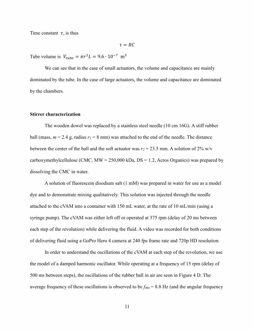
Time constant 𝜏, is thus
𝜏 = 𝑅𝐶
Tube volume is 𝑉𝑡𝑢𝑏𝑒 = 𝜋𝑟2𝐿 = 9.6 ∙ 10−7 m3
We can see that in the case of small actuators, the volume and capacitance are mainly
dominated by the tube. In the case of large actuators, the volume and capacitance are dominated
by the chambers.
Stirrer characterization
The wooden dowel was replaced by a stainless steel needle (10 cm 16G). A stiff rubber
ball (mass, m = 2.4 g, radius r1 = 8 mm) was attached to the end of the needle. The distance
between the center of the ball and the soft actuator was r2 = 23.5 mm. A solution of 2% w/v
carboxymethylcellulose (CMC, MW = 250,000 kDa, DS = 1.2, Acros Organics) was prepared by
dissolving the CMC in water.
A solution of fluorescein disodium salt (1 mM) was prepared in water for use as a model
dye and to demonstrate mixing qualitatively. This solution was injected through the needle
attached to the cVAM into a container with 150 mL water, at the rate of 10 mL/min (using a
syringe pump). The cVAM was either left off or operated at 375 rpm (delay of 20 ms between
each step of the revolution) while delivering the fluid. A video was recorded for both conditions
of delivering fluid using a GoPro Hero 4 camera at 240 fps frame rate and 720p HD resolution.
In order to understand the oscillations of the cVAM at each step of the revolution, we use
the model of a damped harmonic oscillator. While operating at a frequency of 15 rpm (delay of
500 ms between steps), the oscillations of the rubber ball in air are seen in Figure 4 D. The
average frequency of these oscillations is observed to be fobs = 8.8 Hz (and the angular frequency

12
ωobs = 55 rad/s). When assuming an exponential decay (x = e-γt, where x is the displacement, γ is
the damping constant, and t is the time), the damping constant is measured to be γ = 14/s. We can
estimate ω0, the angular frequency if there was no damping using:
𝜔0 = √𝜔𝑜𝑏𝑠2 + 𝛾2 = 57
rad
s
For our system, Newton’s second law can be written in angular terms as:
𝐼𝛼 + 𝑐𝜔 + 𝜅𝜃 = 0
where I is the moment of inertia of the oscillator, α is the angular acceleration, c is the angular
viscous damping constant, ω is the angular frequency, κ is the angular spring constant, θ is the
angular displacement. The moment of inertia I can be calculated using the parallel axis theorem
(and assuming that the mass of then needle is negligible):
𝐼 = 𝑚 (2𝑟1
2
5+ 𝑟2
2) = 1.38 × 10⁻⁶kg m2
The angular spring constant, κ can then be estimated as:
𝜅 = 𝐼𝜔02 = 0.0045 N m rad−1
Using the observed damping coefficient γ, the angular damping constant c (in air, as a result of
both air and elastomer dampening) can be calculated as:
𝑐 = 2𝛾𝐼 = 3.9 × 10⁻⁵ N m s rad−1
We know that viscous drag force is given by:
𝐹𝑑𝑟𝑎𝑔 = 6𝜋𝜂𝑟1𝑣
where is the viscosity of the fluid. Using the relationships, drag = Fdrag r2 (since the angle
between F and r2 is 90°) and v = ω r2, we can write:
𝜏𝑑𝑟𝑎𝑔 = 6𝜋𝜂𝑟1𝑟22𝜔

13
Using drag = c ω, we can estimate the values of viscous damping constant, c in different fluids
using
𝑐 = 6𝜋𝜂𝑟1𝑟22
Thus, cair = 1.7 x 10⁻⁹ N.m.s.rad-1, cwater = 7.4 x 10⁻⁸ N.m.s.rad-1, cCMC = 1.9 x 10⁻⁴ N.m.s.rad-1. We
notice that the constants for air and water are negligible compared to the observed constant for
the elastomer and thus, these fluids do not provide any additional damping effects, whereas for
the CMC solution, the damping constant is one order of magnitude higher than that of the
elastomer and hence increases the damping effects. To verify, we can calculate the parameter c2 -
4Iκ, which determines the nature of solutions to Newton’s second law equation listed above. For
air and water, c2 - 4Iκ < 0 and for CMC c2 - 4Iκ > 0, which corresponds to underdamped and
overdamped cases respectively, as confirmed by Figure 4 D, E.
The power dissipated by the rubber ball due to the work done in a viscous fluid (CMC
solution) can be estimated using the following equation:
𝑃 = 6𝜋𝜂𝑟1𝑣2 = 6𝜋𝜂𝑟1 ((𝑑𝑥
𝑑𝑡)
2
+ (𝑑𝑦
𝑑𝑡)
2
)
where x and y are the position of the ball, and t is the time. The position was extracted from the
videos using a MATLAB program. These estimates of power output were plotted in Figure 4 F
for various frequencies of operation.
Estimating efficiency of actuator
As described in the main text, using the setup shown in Figure 2A, we characterized the
performance of the cVAM when operating with different loads. We added the weights (with mass
m) to the central rod at a distance r = 32 mm. As before, we tracked the position of the rod using
a MATLAB program and measured the following: i) angle of deflection of actuator under
different loads (Figure S 3A), and iii) the maximum actuation angle as the load changes (Figure
14
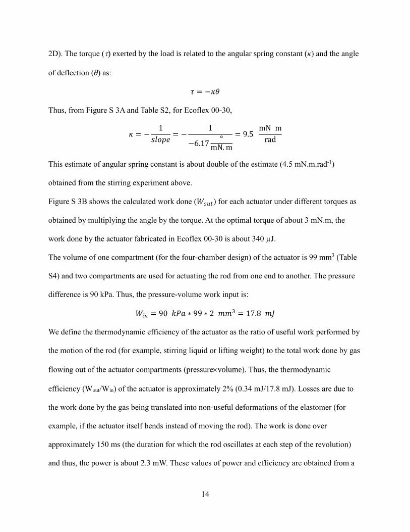
2D). The torque () exerted by the load is related to the angular spring constant (κ) and the angle
of deflection (θ) as:
𝜏 = −𝜅𝜃
Thus, from Figure S 3A and Table S2, for Ecoflex 00-30,
𝜅 = −1
𝑠𝑙𝑜𝑝𝑒= −
1
−6.17°
mN. m
= 9.5 mN m
rad
This estimate of angular spring constant is about double of the estimate (4.5 mN.m.rad-1)
obtained from the stirring experiment above.
Figure S 3B shows the calculated work done (𝑊𝑜𝑢𝑡) for each actuator under different torques as
obtained by multiplying the angle by the torque. At the optimal torque of about 3 mN.m, the
work done by the actuator fabricated in Ecoflex 00-30 is about 340 µJ.
The volume of one compartment (for the four-chamber design) of the actuator is 99 mm3 (Table
S4) and two compartments are used for actuating the rod from one end to another. The pressure
difference is 90 kPa. Thus, the pressure-volume work input is:
𝑊𝑖𝑛 = 90 𝑘𝑃𝑎 ∗ 99 ∗ 2 𝑚𝑚3 = 17.8 𝑚𝐽
We define the thermodynamic efficiency of the actuator as the ratio of useful work performed by
the motion of the rod (for example, stirring liquid or lifting weight) to the total work done by gas
flowing out of the actuator compartments (pressurevolume). Thus, the thermodynamic
efficiency (Wout/Win) of the actuator is approximately 2% (0.34 mJ/17.8 mJ). Losses are due to
the work done by the gas being translated into non-useful deformations of the elastomer (for
example, if the actuator itself bends instead of moving the rod). The work is done over
approximately 150 ms (the duration for which the rod oscillates at each step of the revolution)
and thus, the power is about 2.3 mW. These values of power and efficiency are obtained from a

15
non-optimal actuator. As seen in Table S7, the estimated torque exerted by the actuator is
comparable to theoretical value if the actuator was modeled as a spring coupled to a piston. Yet,
when actuating with a load, energy losses occur due to deformation of the actuator. These losses
could be minimized in future iterations by making the outer walls of the actuator thicker so that
the collapse of the chambers would mostly actuate the rod.

16
Supplementary Tables
Force characterization
Table S1: Elastic moduli of the materials used for fabricating the actuators
Material Elastic modulus (MPa) Source
Ecoflex® (00-30) 0.069 Manufacturer datasheet
Dragonskin® (10 NV) 0.19 Manufacturer datasheet
PDMS (Sylgard® 184) 1.8 Russo et al.1 (2016)
PDMS:Dragnoskin (1:1) 1.0 Calculated as described above
PDMS:Dragonskin (1:3) 0.6 Calculated as described above
Table S2: Characteristics of actuators fabricated in different materials. The slope of deflection
angle 𝜃 vs applied torque 𝜏, when no vacuum is applied (Figure S3A), which is inversely
proportional to the angular spring constant of the actuator 𝜅 (Figure S2). We also report the
slope of maximum actuation angle 𝜑𝑚𝑎𝑥 vs applied torque 𝜏, which is difference between no
applied vacuum and maximum vacuum level (Figure 2D)
Material Slope of deflection angle
𝜃 vs applied torque 𝜏 [˚
/ (mN.m)]. 𝑝 = 0
Slope of maximum actuation angle
𝜑𝑚𝑎𝑥 vs applied torque 𝜏 [˚ /
(mN.m)], p = -90 kPa
Ecoflex (00-30) 6.17 2.23
Dragonskin (10 NS) 5.59 1.97
PDMS:Dragonskin (1:3) 4.12 1.49
PDMS:Dragnoskin (1:1) 3.70 0.78
Table S3: This table supplements Figure S6 and compares actuators with different numbers of
chambers.
3-chamber 4-chamber 5-chamber
Max angle 1 ch (˚) 6.3 8 3.4
Max angle 2 ch (˚) 11.5 16 6.1

17
Sat pressure 1 ch (mbar) -120 -900 -200
Sat pressure 2 ch
(mbar)
-200 -600 -300
Slope (˚/bar) 1 ch 70.4 16.1 25.4
Slope (˚/bar) 2 ch 77.3 31.7 18.5
Table S4: Estimates of time constants for various actuators
Actuator Chamber volume
(10−7m3)
Total capacitance (10−11m3/Pa)
Time constant
(ms)
3-chamber 1.4 1.8 23
4-chamber 0.99 1.8 23
5-chamber 0.75 1.8 23
4-chamber 2x
size
7.9 2.9 38
4-chamber 3x
size
27 6.1 79
Table S5: Part list of the pneumatic control unit for controlling valves. All SMC components
were purchased from Orange Coast Pneumatics (Yorba Lina, CA). Electronic parts were obtained
from Digi-Key Corporation (Thief River Falls, MN)
Component and description Supplier
part number
Source Quantity
IC1. Arduino DUE microcontroller board (32-
bit ARM Cortex-M3 with USB)
1050-1049-
ND
Digi-Key 1
Switching power supply ETSA120330UDC
(CUI Inc.), 120V AC in, 12V 3.3A DC out
T1079-P5P-
ND
Digi-Key 1
T1. N-CH MOSFET transistor IRLZ14. 60V
10A
IRLZ14PBF-
ND
Digi-Key 18
Solenoid valve. Response time: <5ms, flow
conductance: 80mL/(s*bar), electrical power
12V, <100mA.
V114A-
6LOU
SMC 18
Connection wire for valve SY100-30-
4A
SMC 18
Manifold. For mounting 18 valves VV100-S41-
18-M5
SMC 1
Quick-fit connectors. For 4mm tubing with
M5 thread
KQ2S04-
M5A
SMC 20
Quick-fit plug for small tubing. M-04R-2 SMC 3-5

18
Supply Tubing. Polyurethan, OD 4mm, ID
2mm
TUS0425B-
20
SMC Few m
Table S6: Part list of the pneumatic control unit for regulating supplied negative pressure. All
SMC components were purchased from Orange Coast Pneumatics (Yorba Lina, CA). Electronic
parts were obtained from Digi-Key Corporation (Thief River Falls, MN). Digital manometer was
obtained from Total Temperature Instrumentation Inc. (“Instrumart”, S. Burlington, VT)
Component and description Supplier part
number
Source Quantity
IC1. Arduino DUE microcontroller board (32-bit
ARM Cortex-M3 with USB)
1050-1049-ND Digi-Key 1
Switching power supply SDI65-24-U (CUI Inc.),
120V AC in, 24V 2.71A DC out
102-3418-ND Digi-Key 1
IC2. Voltage regulator (LDO) +12V, 1.5A output.
LM340T12
LM340T-12-ND Digi-Key 1
IC3. J-FET operational amplified AD820 AD820ANZ-ND Digi-Key 1
Electronic vacuum regulator. ITV0090-3UBL. 0 to
-1000mbar, +24V power, 0 to 10V control signal
ITV0090-3UBL SMC 1
Digital Pressure Gauge (Manometer). Keller
LEX1 -1to 2 bar, accuracy 0.05% FS
LEX1-2-G1/4 Instrumart 1
Supply Tubing. Polyurethane, OD 4mm, ID 2mm TUS0425B-20 SMC Few m
Table S7: Comparison of values obtained for torque with respect to changes in pressure using an
analytical model and experimental measurements
Material Scale Slope
(˚/mNm)
No vacuum
Initial response
slope (˚/kPa)
Experimental
(µNm/kPa)
Theoretical
(µNm/kPa)
Ecoflex 1 6.2 0.30 48 63
Dragonskin
(DS)
1 5.6 0.24 44 63
PDMS:DS 1:3 1 4.1 0.087 21 63
PDMS:DS 1:1 1 3.7 0.060 16 63
Ecoflex 2 1.9 0.78 410 500
Ecoflex 3 0.72 0.96 1340 1700

19
Supplementary figures
Figure S 1: Fabrication of cVAM. (A) Structure and dimensions (for the 1x model) of the mold
used for making the elastomeric actuators. (B) Process of fabricating cVAMs. The actuator is
fabricated by curing elastomers in a 3D-printed mold. A wooden rod suspended in the mold of
the top piece is bonded into the elastomer when it cures. A support slab is prepared by pouring
elastomer in a tray to obtain a thickness of about 5 mm. A sacrificial tube is placed in the support
slab (by using a biopsy punch to make a hole) while the slab is being attached to the actuator

20
body. After the body and support slab are attached, the sacrificial tube is replaced by pneumatic
tubing.
Figure S 2: Angular spring constant 𝜅 depending on elastic modulus of the material used for
fabricating the actuator.
Figure S 3: This figure extends Figure 2 in the main text. (A) Deflection angle of the rod, when
different loads (torques) are applied, without applying negative pressure. (B) Mechanical work
done by actuators, when different loads are applied. As the maximum actuation amplitude
decreases with increased load, there is an optimal loading torque (around 3 mN.m) for getting

21
maximum work done. Maximum work decreases for actuators fabricated with stiffer elastomers
because they are not completely actuated at atmospheric pressures.

22

23
Figure S 4: The effect of scaling (1x, 2x, 3x) on the performance of actuators. In these cases, all
dimensions of actuators were scaled linearly (1x is the design presented in Figure S1 and used
for testing differences in materials and number of chambers). These actuators had four chambers
and were fabricated in Ecoflex 00-30. (A) Photos of three different scales of actuators next to
each other. (B) Actuation angle depending on applied pressure (no load). (C) Deflection angle
depending on load (no negative pressure). (D) Maximum angle of actuation in the case of
different loads. (E) Maximum mechanical work done by actuators in the case when different
loads were applied. (F) Scaling of angular spring constant 𝜅 depending on size (should scale
cubically with size). (G) Scaling of maximum mechanical work done by actuator (should scale
cubically with size).
Figure S 5: The effect of scaling the actuator on the trajectory and angle of deflection during
revolution. (A) Images showing 1x (the size used for varying materials and number of

24
chambers), 2x, and 3x actuators and their trajectories. (B) The maximum angle of deflection as a
function of frequency of revolution as the actuator is scaled in size.

25
Figure S 6: Hysteresis in actuators as the negative pressure is varied. Pressures are scanned from
0 to vacuum (red) line and back to atmospheric pressure (blue line). We compare different
number of chambers and also the differences between the actuation of one or two chambers.

26
Figure S 7: Schematic layout and image of the valve controller.

27
Figure S 8: (A) Schematic of the electronically controlled negative pressure regulator. (B)
Calibration of the negative pressure to the digital word.
Figure S 9: RC-circuit analog of interfacing the actuator through valve and tubing. This
schematic has been used to develop a crude model for estimating time constants (RC) for the
pneumatic loading of the actuator.

28
Figure S 10: The actuator can fail if the load is too high. Here, the actuator was fabricated in
Ecoflex 00-30 and 4.5mN.m of torque was applied. The rod can detach from actuator because of
the collapse of compartment along the rod’s axis. Thus, the actuator was unable to lift the load as
well and the angle of actuation decreased at high negative pressure.

29
Figure S 11: Dorsal view of the animation of the gait of the reptile Chamaeleo calyptratus. The
frames were extracted from Movie S7 of the work by Fisher et al.3 The time stamps represent the
time elapsed in the video. Schematic illustration of the gait on the top right corner of each frame
represents that the diagonal legs move (almost) simultaneously. Limbs moving forward are
colored in red and limbs applying force backwards are colored in blue.

30
Figure S 12: The amplitude of oscillation remains unchanged for the cVAM actuator after
operating it for over 106 cycles. The top image shows the trajectory (left part of the image shows
the front view of the actuator) and amplitude (right part of the image shows the side view of the
actuator) before the million cycles and the bottom image shows the actuation after the million
cycles.

31
Supplementary videos
Movie S1 A single actuator moves the rod by 16° when vacuum is applied.
Movie S2 Demonstration of stirring with plastic beads.
Movie S3 Characterization of the cVAM for different frequencies of operation and different
pressures.
Movie S4 Demonstration of stirring while delivering fluid using cVAM.
Movie S5 A four-legged “walker” that is operated by the action of four cVAMs.
Movie S6 A propped up view of the four-legged “walker.”
Movie S7 The movement of a single actuator in the “walker.”

32
References
1. Russo S, Ranzani T, Gafford J, Walsh CJ, Wood RJ. Soft Pop-up Mechanisms for Micro
Surgical Tools: Design and Characterization of Compliant Millimeter-Scale Articulated
Structures. IEEE Int Conf Robot. 2016: 750-757.
2. Yang D, Verma MS, So J-H, Mosadegh B, Keplinger C, Lee B, Khashai F, Lossner E,
Suo Z, Whitesides GM. Buckling Pneumatic Linear Actuators Inspired by Muscle. Adv
Mater Technol. 2016; 1(3): 1600055.
3. Fischer MS, Krause C, Lilje KE. Evolution of Chameleon Locomotion, or How to
Become Arboreal as a Reptile. Zoology. 2010; 113(2): 67-74.


