


M.I.T. LIBRARIES - DEWEY

Digitized by the Internet Archive
in 2011 with funding from
Boston Library Consortium Member Libraries
http://www.archive.org/details/superstarsinnbaeOOhaus

HB31.M415
working paper
department
of economics
SUPERSTARS IN THE NBA: ECONOMIC VALUE AND POLICY
Jerry A. HausmanGregory K. Leonard
95-2 Sept. 1994
massachusetts
institute of
technology
50 memorial drive
Cambridge, mass. 02139


SUPERSTARS IN THE NBA: ECONOMIC VALUE AND POLICY
Jerry A. HausmanGregory K. Leonard
95-2 Sept. 1994
MASSACHUSETTS INSTITUTE
OF TECHNOLOGY
MAR 2 9 1995
LIBRARIES


95-2
SUPERSTARS IN THE NBA: ECONOMIC VALUE AND POLICY
Jerry A. Hausman, MITGregory K. Leonard, Cambridge Economics
ABSTRACT
Two competing arguments have been put forward regarding the extraordinary fan interest in
sports leagues. The first argument is based on the concept of "superstars," asserting that fan
interest is generated by the desire to see great players exhibit their skills. The second
argument, called "competitive balance," is defined as the condition that prevails when the
disparity between the best and worst teams in a league is not too great. We investigate the
effects of superstars on fan interest and the revenues of NBA teams. In particular, weanalyze the impact superstars have on attendance and television ratings and show that, in
addition to the effect they have on their own teams, superstars exert a tremendous positive
externality on other teams. The NBA and NFL have adopted salary cap policies to avoid the
problems caused by the superstar externalities and maintain competitive balance. Wedemonstrate that a salary cap is typically not the economically efficient way to achieve the
goals of competitive balance and the financial viability of small market teams. Instead, weshow that the league should impose a tax on superstar salaries. We show that the tax is less
distortionary than the salary cap.

Preliminary
Please Do Not QuoteSeptember 1994
Superstars in the NBA: Economic Value and Policy1
Jerry A. Hausman, MITGregory K. Leonard, Cambridge Economics
L Introduction
The major US sports leagues are extremely popular with consumers who spend approximately $1.5
billion to attend live professional sporting events and television advertisers who spend over $2.5 billion to
reach viewers of televised sporting events. Two competing (but not necessarily mutually exclusive)
arguments have been put forward regarding the extraordinary fan interest in sports leagues. The first
argument is based on the concept of "superstars," asserting that fan interest is generated by the desire to see
great players exhibit their skills. The second argument, based on what is called "competitive balance," has
been put forward by sports leagues engaged in labor and antitrust disputes.2 "Competitive balance" is
loosely defined as the condition that prevails when the disparity between the best and worst teams in a
league is not too great. "Parity" is another word that is commonly used to describe this condition.
Leagues argue that competitive balance is vital to a sport league's success. With competitive
balance, the argument goes, the outcome of every game is in doubt, creating excitement and interest on
the part of the league's fans. This excitement and interest translates into increased attendance, television
ratings, and sports paraphenalia purchases, all of which increase the revenues of the league's teams.
Without competitive balance, the sports leagues claim that fan interest will wane, jeopordizing the
existence of low revenue teams, or even the entire league. In the labor and antirust disputes, the leagues
1 The authors consulted for Chicago television station WCN and the Chicago Bulls in their antitrust suit
against the National Basketball Association. The issues in this paper are not directly related to the issues in
the lawsuit. All views expressed are ours and not necessarily those of WCN and the Bulls. We thank Peter
Diamond for helpful discussions and Tomomi Kumagai, Karen Hull, and Ling Zhang for excellent research
assistance.
2See, e.g., the recently litigated "McNeil" case.

have argued that league-instituted restrictions on player movement, such as the draft and limits on free
agency, and the teams' ability to compete with each other, such as territorial restrictions, are simply ways
to maintain competitive balance.
The National Basketball Association (NBA) is currently the model for a successful sports league.
As recently as the late 1970's, however, the NBA had serious difficulties with drug scandals, declining
attendance, and little interest from the national television networks. 3In 1983, one year prior to the
ascension of David Stern to commissioner, an innovative collective bargaining agreement was reached by
the NBA and the Players' Association. The agreement contained, among other provisions, a drug policy, a
salary cap, and a guarantee from the teams that the players would receive at least 53% of gross revenues.
The resurgence of the NBA has frequently been attributed to the collective bargaining agreement with its
provisions for improving competitive balance. Indeed, the other sports leagues have recently begun to
enact league policies similar to those of the NBA. For instance, the National Football League (NFL) has
recently adopted a salary cap system.
The collective bargaining agreement was not the only important NBA event to occur in the late
70's and early 80's. In 1979, Larry Bird and Magic Johnson entered the NBA after having played against
each other in the 1979 NCAA Championship game, which is still the highest rated college basketball game
in history. Starting from that season, a succession of NBA superstars emerged-from Bird and Magic to
Michael Jordan, who entered the NBA in 1984, to Shaquille O'Neal, who entered in 1992. Basketball is a
sport well-suited for the development of superstars. Players are highly visible to fans because they do not
wear headgear, only five players are on the floor at any one time, and fans are close to the action. In
addition, although basketball is a team game, individual players can make spectacular individual plays.
The advantage that NBA players have over players from other sports is demonstrated by the success NBA
superstars have had in obtaining endorsements.
Recent developments suggest that superstars are more important than competitive balance. The
3 The last game of the 1980 NBA championship series was televised on tape delay at 1 1:30 pm.
Contrast this treatment to the 1993 NBA Finals, where each game was shown in prime time.

1993 NBA Finals, which featured Michael Jordan, averaged a 17.9 Nielsen television rating (meaning that
an estimated 17.9% of television households watched each game on average). The 1994 NBA Finals,
however, averaged only a 12.2 rating despite the presence of the New York Knicks, a team playing in the
largest Nielsen market. Although the NBA was well-balanced that season, with a number of teams thought
to be contenders for the NBA championship, Michael Jordan had retired and Larry Bird and Magic Johnson
were long since gone.
Thus, the superstar theory suggests itself as a powerful alternative argument to the competitive
balance theory. Indeed, given the emergence of superstars in the NBA at the same time the league office
was orchestrating structural changes in the way the league operated, a natural question to ask is whether
the NBA's revival was due to competitive balance, as is frequently asserted, or, alternatively, to the
emergence of superstars. It seems quite plausible that fans are more likely to watch NBA games with
superstars, regardless of competitive balance. We investigate the effect of superstars on fan interest and
the revenues of NBA teams. In particular, we analyze the impact superstars have on attendence and
television ratings and show that, in addition to the effect they have on their own teams, superstars exert a
tremendous positive externality on other teams.
We also demonstrate that a superstar exerts a positive externality within his own team. Sports
commentators frequently discuss how true superstars "make the players around them better." We
characterize this superstar effect as a form of increasing returns to scale or a positive externality. This
effect is somewhat different than the superstar effect analyzed by Rosen (1981). There, average quality is a
poor substitute for superstar quality and a few superstars can serve many consumers. Thus, superstars
receive large compensation and "produce" most of the good. Here, we are focussing on a different aspect
of the production technology, as described above. With the two types of externalities generated by
superstars, paying salaries to players equal to their marginal revenue product could lead teams, especially
small market teams, into financial difficulties.
The NBA and NFL have adopted salary cap policies to avoid the problems caused by the superstar
externalities and maintain competitive balance. We demonstrate that a salary cap is typically not the

economically efficient way to achieve the goals of competitive balance and the financial viability of small
market teams. Instead, we show that the league should impose a tax on superstar salaries. We show that
the tax is less distortionary than the salary cap.
IL The Salary Cap, the Draft, and Competitive Balance
The success of the NBA over the last 15 years has been accompanied by a substantial increase in
player salaries. In the 1991-1992 season, the average NBA player was paid approximately $1 million,
about three times the average salary in the early 1980's. Superstar players, of course, are paid even
greater amounts than the average player. When he retired prior to the 1993-1994 season, Michael
Jordan's salary from the Chicago Bulls was about $3 million per season and his professional earnings,
including endorsements, totalled about $35 million. In the last several years, a number of emerging
superstars, like Larry Johnson of the Charlotte Hornets, have received long term contracts with total
payments amounting to nearly $100 million.
The collective bargaining agreement between the NBA and the Players' Association allows the
league to impose on each NBA team a salary cap which limits the total amount the team can spend on
player salaries. In return for this concession, the NBA guaranteed that 53% of gross revenues would go to
the players. Also, the salary cap system has a complication: a team can enter contracts with its current
players at salary levels which put the team above the cap." Only a "base" amount of a current player's
salary counts toward the cap. If, on the other hand, a team wants to enter a contract with a free agent (or
a draft pick), the full amount of the salary would count toward the cap. Thus, the cap prevents teams from
"raiding" the rosters of other teams. For instance, if the Boston Celtics wanted to obtain Shaquille
O'Neal's services (assuming he were a free agent), their salary offer would be limited by the cap. The
4 Teams have recently attempted to take advantage of this complication using so-called "one year and
out" contracts. Under such a contract, a team signs a free agent to a contract (at a salary under the cap)
which gives the player the option of free agency after one year. At that time, the team can resign the player
at a much higher salary, now unrestricted by the cap.

Orlando Magic's ability to meet the Celtics' offer, however, would not be impeded by the cap.
The NBA has argued that the salary cap and the draft are necessary to create competitive balance
since teams have revenue streams that differ according to city size and other factors. While the revenues
generated by the NBA's national TV contracts are shared equally among the teams, the revenues generated
by a team in its local territory, such as live gate, local TV, and local radio, are not shared with the other
teams. Thus, teams with large local territories, such as New York, may have higher revenue streams than
teams with relatively small local territories, such as Sacramento. 5
The NBA draft distributes entering talent to teams according to descending order ot existing team
quality, as measured by win-loss record. Thus, players entering the NBA are not allowed to take their
services to the highest bidder, a restriction which prevents high revenue teams (which may otherwise have
a low draft position) from buying up the most talented players entering the league. Meanwhile, the salary
cap limits the ability of the high revenue teams from bidding away existing talented players from the low
revenue teams. Thus, the draft and salary cap are thought to allow small city teams, which have lower
revenue streams, to obtain and retain talented players which, in turn, allows them to compete on the court
with large city teams.
Economists working for the various players' associations have argued that the draft must be
irrelevant for competitive balance because the Coase theorem implies that the endowments (i.e., the draft
positions) do not affect the final allocation of players. Although this argument may have certain merits
when applied to major league baseball and, until recently, the NFL, it does not apply to the NBA because
the salary cap creates a transactions cost (a team's payroll cannot exceed the cap). Thus, the draft
combined with the salary cap does have the potential to increase competitive balance in the NBA and
support small market teams. 6 We address the question of whether the salary cap is the most economically
5 Of course, some small city teams like Portland have generated large revenue streams.
6Note, however, that economic inefficiency results. Michael Jordan's marginal value in Chicago was
likely greater than it would have been in Sacramento. If Sacramento had drafted Jordan and the salary cap
had prevented Chicago from trading for him, the result might have been a loss in efficiency. Thus, we see
that the salary cap is most likely a way to transfer wealth from the players to the owners. These points are
also discussed by Quirk and Fort (1992).

efficient way to support small market teams in the last section. In the next two sections, we measure the
extent of the superstar effect on league revenues and attempt to determine the relative importance of
competitive balance.
III. The Superstar Effect on League Revenues
A superstar can have an impact on the revenues of his own team in at least three ways. First, the
superstar directly increases the quality of his own team. The increased quality of the team presumably
attracts more fans. Second, the superstar indirectly increases the quality of his own team by making the
players around him better. This indirect effect can be characterized as a positive externality. Third, the
superstar may have a "personal appeal" that attracts fans even after controlling for his team's (increased)
quality.
A superstar will generally increase other teams' revenues as well as his own team's revenues. The
effect of the superstar on other teams' revenues is a positive externality in the sense that the other teams
receive the benefit, but do not contribute towards paying the superstar's salary. In what follows, we
attempt to measure the size of the effect superstars have on various sources of team revenue.
A. Gate Revenue
We start by estimating the effect of a superstar on his own team's attendance. This effect can be
roughly estimated by comparing the team's home attendance in the season prior to the arrival of the
superstar to subsequent seasons (assuming that the quality of the other players on the team remains the
same). 7 We subsequently estimate the effect a superstar has on other teams' revenues by comparing the
other teams' home attendance for games against the superstar's team to their average attendance against
other teams. In estimating the superstar effects, we focus on two of the most prominent NBA superstars in
7This analysis also does not fully account for any price increases that the teams may be able to
charge.

the 1980's, Larry Bird and Michael Jordan.
Larry Bird had a substantial impact on the attendance of Celtics games at the Boston Garden after
his entrance into the NBA. In the 1978-1979 season, a year before Bird's arrival, the average attendance
per game was approximately 10,000. Starting in Bird's second season and lasting until his retirement, the
Boston Garden was sold out for every game (capacity is about 15,000). Thus, attendance increased by
about 50% during the Bird era. In the 1993-1994 season, the second since Bird's retirement, home games
no longer sell out and the number of season ticket holders is declining. These comparisons must be
viewed with some degree of caution, however, since the Celtic teams prior to Bird's arrival and after his
retirement have been of very different composition, apart from Bird, than the Celtic teams during his
career.
Like Larry Bird in Boston, Michael Jordan had a huge effect on attendance at Chicago Stadium.
The Bulls average attendance was about 6,000 per game the season before Jordan arrived. Average
attendance doubled in his first year, and every game in Chicago Stadium sold out during the six seasons
prior to Jordan's retirement (Chicago Stadium holds about 18,000). Of course, some of the attendance
increase may be due to a "championship" effect since the Bulls were the NBA champions for the three
seasons ending with the 1992-1993 season. In the 1993-1994 season, the first season after Jordan's
retirement, home games have continued to sell out, but team is still of high quality and indeed still has
Scottie Pippen who was a Dream Team member and is an All-Star player. Also, to some extent season
ticket holders may be unwilling to give up their seats in anticipation that Jordan might yet return to the
Bulls. If we conservatively estimate the Jordan attendance effect by the increase of 6,000 per game in
Jordan's first year and we assume that the incremental tickets were sold at the average ticket price, Jordan
increased the Bulls' gate revenue by about $8.6 million.
The effect of a superstar on the gate attendance of other teams can be measured by comparing the
attendance of the superstar's road games to average road attendance. In other words, we ask whether the
superstar's team draws better on the road than other teams. Because stadiums have capacity constraints,
the observed superstar effect may underestimate the potential superstar effect. Even so, we find the

observed superstar effect to be quite large.
Several facts point to the existence of a substantial Michael Jordan effect on road attendance. In
the 1989-1990 season, ail but one Bulls road game was sold out.8
In the 1990-1991 and 1991-1992
seasons, every Bulls road game was sold out. Since NBA teams' average attendance is less than full
stadium capacity, Jordan was certainly having an effect on other teams' attendance.
We examine more closely the attendance data for the 1989-1990 and 1991-1992 seasons to
estimate the size of the Jordan and Bird effects on attendance and gate revenue. In the first two columns
of Table 1, we give by NBA team the average 1989-1990 home attendance for games against the Bulls and
for games against other teams. The attendance for Bulls games was higher than for non-Bulls games for
every team except three (Detroit, Boston, Sacramento) where stadium capacity constraints were binding
even for non-Bulls games. For some teams, the increase in the attendance was enormous. Washington
Bullets attendance almost doubled when. playing the Bulls, while the Indiana Pacers and New Jersey Nets
attendance went up by about 50% when playing the Bulls. The third column of Table 1 presents for each
team an estimate of the incremental revenue due to the Bulls. Since a team's gate revenue for each game
is not shared with the visiting team, the estimated incremental revenue accrued directly to the indicated
team. Thus, Washington, a team that has not had a good win-loss record in some time, received an
additional $250,000 due to having the Bulls and Michael Jordan visit their stadium once a year. Summing
across teams, the incremental revenue due to the Bulls is estimated to be $1.6 million. Table 2 presents
similar information for the 1991-1992 season. The estimate of incremental revenue for other teams due to
the Bulls is $2.5 million. Tables 3 and 4 present information on the Celtics' incremental attendance effects
in the 1989-1990 and 1991-1992 seasons. The incremental revenue effects are estimated to be $1.4
million and $2.1 million respectively.
8 The New Jersey (Exit 16W) Nets were the single "offender".
8
B. Superstar Effect on Television Ratings
In addition to being a draw for gate attendance, superstars may draw viewers to televised NBA
games, raising the television ratings of these games. Thus, we investigate whether, holding other factors
constant, television ratings are higher for games featuring a superstar. Among the factors that can be held
constant are the qualities of the teams involved, which allows us to compare the relative importance for
television ratings of showing a game involving "good" teams versus showing a game involving a superstar.
There are four types of telecasts through which an NBA game can reach television viewers. Two
of the telecast types are "national" in nature while the other two are "local." First, the game could be
broadcast nationally on the NBA's national over-the-air (OTA) network, which is currently the National
Broadcasting Corporation (NBC). Second, the game might be telecast nationally on the NBAs national
cable network, which is currently Turner Network Television (TNT). Third, the game might be broadcast
locally in the territory of one of the teams involved by a local OTA outlet Such a broadcast is called a
"local OTA telecast".9
Finally, the game might be telecast locally in the territory of one of the teams
involved by a local cable outlet. Such a telecast is called a "local cable telecast".
The NBA, acting as agent for the 27 teams, negotiates the national OTA and national cable
packages. The revenues derived from these national network contracts are divided equally among the
teams. Each team is responsible for negotiating its own local cable and local OTA packages. Most NBA
teams have contracts for both types of television distribution.
The NBA has instituted a number of league rules which restrict the manner in which NBA games
can be televised. NBC is given first choice of which games to televise and shows about 20-25 regular
season games per season, mostly on weekend afternoons. League rules prohibit the telecast (local or
national) of any other NBA game within two hours of an NBC telecast. Thus, NBA on NBC telecasts face
no competition from other NBA telecasts. TNT is given second choice of games and shows about 51
9Several teams, notably the Chicago Bulls and Atlanta Hawks, have local broadcast outlets which are
also so-called "superstations". Superstations are local channels whose signal is picked up by a third-party
carrier and sent via sattelite to local cable systems throughout the US. Thus, Bulls games shown locally on
WCN and Hawks games shown locally on WTBS end up being transmitted to other parts of the country.

regular season games per season, mostly on Tuesday and Friday nights. Starting with the 1990-1991
season, a league rule was instituted which prohibits superstations from telecasting NBA games on the same
night as TNT. However, teams are still allowed to telecast their own games locally, via either OTA or
cable, at the same time TNT is televising a game. Thus, TNT is given only limited protection from
competing NBA telecasts. Given the selection by NBC, local teams can choose how to allocate their
remaining games between their local OTA and cable telecasters. However, a league rule limits the
number of games which can be shown over-the-air to a maximum of 41.
We use TV ratings data from the 1989-1990 and 1991-1992 seasons to analyze the impact of
superstars on the ratings of televised NBA games. The data include information on a large number of
national OTA, national cable, local OTA, and local cable telecasts. In the 1989-1990 season, the Detroit
Pistons were the defending champions, having defeated the Los Angeles Lakers in the previous season's
NBA Finals. The Chicago Bulls featured Michael Jordan, the Boston Celtics featured Larry Bird, and the
Los Angeles Lakers featured Magic Johnson. In our analysis, we focus on these three superstars, plus Isiah
Thomas of the Pistons.10
In the 1991-1992 season, the Bulls were the defending champions, having
defeated the Lakers in the previous season's Finals. We investigate the way in which the two seasons
differ in terms of superstar effects.
2i Local OTA Ratings
When a team broadcasts one of its games locally into its Designated Market Area (DMA)" using a
local broadcast station, the telecast is called a "local over-the-air telecast". An example of a local OTA
telecast is the broadcast by Boston independent channel WLVI of the December 5, 1989 Celtics-Charlotte
game. A single game may be the source for two local OTA telecasts, one by each team in its respective
,0 Thomas' stature as a superstar may not have been as great as the other three, but the Pistons as
defending champions and "bad boys" may have had appeal as a team.
" DMAs are defined by Nielsen and generally encompass a city and its environs.
10

DMA. 12In this case, the two telecasts would represent separate OTA telecast observations in the data,
each with its own rating. The ratings data for the 1989-1990 and 1991-1992 seasons were obtained from
Nielsen. For the 1989-1990 season, we have data on 598 local OTA telecasts. For the 1991-1992 season,
we have data on 608 local OTA telecasts. At least one telecast from each NBA team is included in the
data, except for the New York Knicks which had no local OTA telecasts.13
We considered the observable factors which might determine the rating received by a game
telecast. First, because we have panel data (more than one game for each telecasting team), we include a
fixed effect for each telecasting team.'4 Second, because viewer availability can vary depending on when
the game is played, we control for day of the week, month, start time of the telecast, and the rating of the
half-hour on the telecasting station leading into the game telecast. Start time, in particular, is considered
by television programmers to be an important determinant of ratings, with "late starts" getting lower ratings
because some viewers may be unwilling to forego sleep for televised basketball.
Third, we control for the presence of "competing" NBA telecasts. Telecasts of NBA games by
national NBA cablecaster TNT or superstations WGN and WTBS can overlap with the local OTA telecast,
providing viewers with an alternative NBA telecast. To account for these competing telecasts, we interact
the fraction of the OTA telecast that is overlapped by the TNT (or superstation) telecast with the cable
penetration of TNT (or the superstation) into the local DMA. Controlling for channel penetration is
particularly important for superstations since, for instance, WGN has limited penetration into certain parts
of the country such as the northeast.
Fourth, we control for the effect of the opponent's quality by including the opponent's win/loss
percentage. Finally, we account for the superstar effect by including four indicator variables that indicate
12Or, of course, two local cable telecasts, or one local cable and one OTA telecast.
13 The Knicks telecast locally over MSG, which is a cable channel.
MBecause the New York and Los Angeles DMAs each have two teams, the fixed effects are for the
telecasting teams, not the DMAs.
11

whether the opponent's team is the Celtics, Bulls, Lakers, or Pistons respectively.'5 Table 5 gives the
means of the variables used in the model by season.
The cable household television rating reported by Nielsen is defined as the number of cable TV
households with televisions tuned to the game divided by the total number of cable TV households in the
DMA. Thus, the rating is bounded between zero and one. In order to account for this characteristic of
the left-hand-side variable, we specify the following functional form for the expectation of the television
rating Ri;of team i's telecast of game j, conditional on X
i;and a,
16
E(Rg\X9 , ai) = F(Xy{l + a,) (D
where X;j
- are the variables that vary across team and game, a, is the fixed effect for telecasting team i, and
FO is a cumulative distribution function. In what follows, we assume the logit cdf.'7 We estimate the
parameters in specification (1) using quasi-maximum likelihood where the likelihood for an observation is
specified as the Bernoulli likelihood
L, = [F(Xyfi + a )]*> [1 - F(Xft + a^-** (2)
The quasi-maximum likelihood estimates (QMLE) of (3 and the a, are consistent as long as the conditional
expectation (1) is correctly specified even if the Bernoulli specification (2) is incorrect.'8 The asymptotic
variance-covariance matrix of the QMLE estimates is estimated maintaining only first moment assumptions
' 5 Of course, the superstar effect cannot be identified separately from any team effect (e.g., a Celtics
effect) that might be present after controlling for win/loss percentage.
,6See Papke and Wooldridge (1993) for more details regarding this approach.
17 The use of the normal cdf leads, of course, to similar results.
18There is no incidental parameters problem with fixed effects here because the number of teams is
assumed fixed while the number of observations per team is assumed to go to infinity.
12

(1) without any additional second moment assumptions.
a. The 1989-1990 Local OTA Results
For reasons discussed further below, we estimate separate models for the two seasons for which
we have data. The estimated coefficients for the 1989-1990 season are provided in Table 6. One
surprising result is the relative unimportance of the opponent's win/loss percentage. The estimated
coefficient on win/loss percentage is only 0.047 and a t-test does not reject the hypothesis that it is zero.
Thus, controlling for superstar effects, the quality of the opponent appears to have little effect on ratings.
For instance, at the mean of the data, a rating increase of only 2% would result if the telecasting team
were playing against an opponent with a 0.750 win/loss record instead of a 0.250 win/loss record.
The superstar effects, on the other hand, are quite important determinants of ratings. The
coefficients on the superstar team dummy variables are estimated to be positive and large and they are
estimated with a high degree of precision. We find that Isiah Thomas has only a small effect on ratings
(8% increase), while the Michael Jordan and Larry Bird increase ratings by 24% and 21% respectively.
Magic Johnson has the largest effect on ratings, raising them by 31%.' 9
The other variables in the model generally have an impact on ratings consistent with the beliefs
commonly held in the sports TV industry. Late starts do poorly relative to earlier starts, with a 7-7:30 start
receiving the best ratings on average. Telecasts in November (the opening month of the season) receive
the highest ratings, while telecasts in December receive the lowest ratings. The day of the week variables
do not have very precisely estimated impacts on ratings, although the result for Saturday is consistent with
the view that Saturday is a poor night for television ratings generally and sports telecasts in particular.
b. The 1991-1992 Local OTA Results
The 1991-1992 OTA results are given in Table 7. In some ways, these results are similar to the
19 These estimates of percentage increase in rating are calculated from the estimated coefficients and
the underlying data.
13

1989-1990 results. The 7-7:30 start time again receives the highest ratings among start times, November
telecasts receive higher ratings than other months, and Saturday is not a particularly strong night for
ratings. Also, the opponent's winning percentage again has a small and imprecisely estimated impact on
ratings.
However, the estimated superstar team effects differ substantially from those in the 1989-1990
results. The Bulls with Michael Jordan now increase ratings by 45%, which is even higher than the Bulls
effect in the 1989-1990 season. On the other hand, the 1991-1992 effects for the Celtics and the Lakers
are much smaller than their 1989-1990 effects (5% each). The explanation for the difference is that Magic
Johnson had retired and Larry Bird played in only 45 of 82 games in the 1991-1992 season. When he did
play, it was usually in great pain and with lessened effectiveness. Thus, the Celtics and Lakers played the
1991-1992 season essentially without their superstars, which reduced their viability as television
attractions.
The 1989-1990 results and the Bulls 1991-1992 result suggest the presence of a powerful
superstar effect, controlling for the quality of the opponent. The comparison between the results for the
two seasons provides even more evidence that superstars have a substantial effect on ratings. We note
that the estimated superstar effect applies to the local OTA ratings of teams other than the superstar's.
Since a team's local TV revenues are not shared with the other teams20, and television revenues depend
crucially on season average ratings, teams with superstars produce a large positive externality for teams
without superstars.
2. Local Cable Ratings
When a team telecasts locally into its DMA using a local cable network (for instance, a regional
sports network), the telecast is called a "local cable" telecast. An example of a local cable telecast is the
distribution by SportsChannel New England (a regional sports network) in the Boston area of the
December 6, 1989 Celtics-Knicks game. As with local OTA, we obtained from Nielsen ratings data for
20 Aside from a payment of 6% to the NBA league office.
14

local cable telecasts in the 1989-1990 and 1991-1992 seasons. For the 1989-1990 season, we have 583
observations, while for the 1991-1992 season, we have 654 observations. Data for seventeen of the 27
NBA teams appear in the local cable dataset.21
As with the local OTA model, the conditional expectation for the local cable rating is specified
according to equation (1). The specification includes fixed effects for the telecasting teams; variables for
day of week, month, start time, and rating of the lead-in program; controls for competing NBA telecasts;
opponent's winning percentage; and the superstar effect variables. Means of the variables used in the
model are given in Table 8. Note that the average rating of a local cable telecast is well below that of a
local OTA telecast (2.9% versus 6.2% in the 1989-1990 season). One reason for the lower rating is that
regional sports networks are typically on an upper tier on local cable systems, requiring subscribers to pay
an extra fee to receive the service.
a. The 1989-1990 Local Cable Results
The results of the 1989-1990 local cable model, given in Table 9, differ in several important ways
from the local OTA results. In contrast to the local OTA model, a higher quality opponent, as measured
by the win/loss percentage, leads to higher ratings for a local cable telecast. The estimated effect of
increasing the opponent's win/loss percentage from 0.250 to 0.750 is to increase the rating by 17%. On
the other hand, the superstar effects are much less important here than in the local OTA model. Only the
estimated Bulls/Jordan effect has a relatively large magnitude, leading to a 20% increase in rating.
b. The 1991-1992 Local Cable Results
The results for the 1991-1992 local cable model are given in Table 10. As with the 1989-1990
season, of the superstar effects, only the Bulls/Jordan effect has a sizable magnitude. The Bulls/Jordan
increase ratings by 30%. However, the effect is estimated somewhat imprecisely. The coefficient on the
opponent's win/loss percentage is estimated to be only half as large as the 1989-1990 coefficient.
21 Some NBA teams do not have a local cable contract and thus do not have local cable telecasts.
15

Nevertheless, these results provide more support for the conclusion that the quality of the opponent is a
more important determinant of cable rating than OTA rating.
The difference between the OTA and cable results may be due to differences in the potential
audiences of the cable and OTA telecasts. Many cable telecast viewers have to pay for the service. Thus,
they are likely to be viewers with stronger preferences for NBA basketball. Such viewers may be less
swayed by the appearance of a superstar than the more casual NBA viewers who constitute a large fraction
of the OTA telecast audience.
Although the superstar externality is smaller with regard to local cable ratings, local cable
revenues typically make up a much smaller share of total local TV revenue than local OTA revenues. 22
Thus, the large externality demonstrated by the OTA results will have a large effect when overall local TV
revenues are considered.
3. TNT Ratings
When TNT telecasts an NBA game, it sends the game via satellite to local cable systems
throughout the country. Since TNT reaches about 60% of cable TV households, it is considered a
"national" cable network and its telecasts are thus considered "national." Unlike regional sports networks,
TNT is typically available to basic cable subscribers without an additional fee. Data on TNT cable
household ratings in the 25 DMAs with NBA teams were obtained from Nielsen. For each DMA, ratings
are available for up to 50 TNT regular season telecasts. The total number of observations in the TNT
dataset is 1035.
As with the local OTA and cable models, we use equation (1) to specify the conditional
expectation of the TNT rating. However, the TNT model differs from the local television models with
respect to the included right-hand-side variables. In addition to the day of week, month, start time, and
22 The exceptions are the New York Knicks, who do not have a local OTA package, and the Los
Angeles Lakers, who have an exceptionally lucrative local cable package.
16

superstar variables, the competing NBA telecast variable is defined somewhat differently and several
additional variables were required.23 With regard to competing NBA telecasts, the most important
competing telecasts are local OTA and cable telecasts. If the team associated with a DMA is televising a
game locally at the same time TNT is televising a game, TNT's rating in that DMA might be lower since
many viewers will prefer to watch their local team over the two teams playing on TNT. The other type of
competing telecast to consider is a superstation telecast. Viewers may prefer to watch the Bulls play on
WCN rather than the two teams playing on TNT. 24
Three additional controls are included in the TNT specification. First, an indicator variable is
included to account for whether the DMA's team was involved in the TNT game. The TNT rating is likely
higher in the DMAs of the two teams playing than elsewhere. Second, an indicator variable is included
for whether the TNT game was part of a TNT doubleheader. The third set of additional variables controls
for the winning percentages of the two teams involved in the TNT game. The competitive balance
argument suggests that when the teams' winning percentages are high and similar, interest in the game
should be higher than when they are quite disparate. We first characterized each team as having a "high"
(greater than 0.600), "medium" (between 0.400 and 0.600), or "low" (below 0.400) winning percentage.
For each TNT game, we determined whether the game involved two "low" teams, one "low" team and
one "medium" team, etc., creating an indicator variable for each possibility. The resulting indicator
variables were included in the specification, with the "high, high" case the excluded dummy variable.
Table 1 1 gives the means of the variables used in the analysis.
The TNT results, given in Table 12, demonstrate that the winning percentage variables do not
have the impact on TNT rating suggested by the competitive balance theory. The "high, high" case, where
23 The definition of the superstar effect variables is slightly different for the TNT model. Here, the
superstar effect variables are dummy variables set to one if the Celtics, Bulls, Lakers, or Pistons,
respectively were one of the two teams playing in the TNT game. In the local OTA and cable models, the
dummy variables are set to one only if the team opposing the local team was one of the above teams.
24 Competition between superstation telecasts and TNT occurring on the same night has been banned
since the 1989-1990 season by a league rule which prohibits superstations from telecasting an game the
same night that TNT telecasts a game.
17

the winning percentages of both teams are above 0.600 does not even yield the highest rating. Games
where the teams are both of the same type and are thus "competitive," do not have higher ratings on
average than games where there is a disparity between the teams. Superstars, on the other hand, have a
tremendous effect on the TNT rating. Isaiah Thomas has the smallest effect, raising the TNT rating by
13%, while Larry Bird has a 32% effect and Michael Jordan has a 25% effect. Magic Johnson's effect is
quite large, raising TNT's rating by 48%. With superstars appearing in 30 of the 51 TNT telecasts during
the 1989-1990 season, we estimate that superstars accounted for over 19% of total TNT regular season
gross ratings points.
With TNT, superstars again exert a large positive externality. The rights fee paid by TNT to the
NBA is split equally among the NBA teams. The size of the rights fee depends in general upon the
amount of advertising revenue TNT can generate, which in turn depends upon the ratings NBA games can
deliver on TNT. Thus, when the presence of Michael Jordan produces higher TNT ratings, all NBA teams
benefit even though the Bulls are paying his salary.
4. NBC Ratings
NBC is currently the national OTA network of the NBA. We have Nielsen data on the ratings of
NBA games on NBC for the 1990-1991 through the 1992-1993 seasons. Unfortunately, the data here are
less rich than the data used in the TNT model in the sense that we have only the overall national rating for
each telecast, not the ratings separately for a set of DMAs. However, it is still possible to estimate
superstar effects with reasonable precision.
During the three seasons for which we have data, NBC telecast games primarily on weekend
afternoons. NBA rules prohibit any other NBA telecasts from competing with the NBA on NBC telecasts.
Thus, we again employ the specification given by equation (1), but with a smaller set of right-hand-side
variables. In particular, we control for start time, day of week, month, and season; the presence of NCAA
(college basketball) Tournament telecasts; and superstar effects for the Bulls, the Celtics (during the first
two seasons when Bird was still playing), and the Lakers (during the first season when Johnson was still
18

playing).25 The means of the variables are given in Table 13.
The results for NBC are given in Table 14. As in the previous models, the Bulls/Jordan have a
large effect on ratings, increasing the NBC rating by 36%. The Celtics with Bird and the Lakers with
Johnson were also strong draws for viewers, increasing the NBC rating by 36% and 19% respectively. If
indicator variables for the Celtics and Lakers are included for the seasons when Bird and Johnson are no
longer playing, their estimated coefficients are small and not statistically significant from zero, which is
somewhat surprising given the nationwide following received by the Celtics and Lakers. Thus, this result
further demonstrates the strong superstar effects on television ratings.
C. The Value of Michael Jordan to Other NBA Teams
We now estimate the value of Michael Jordan to NBA teams other than the Chicago Bulls by
estimating the incremental revenue he generates for those teams. Four of the largest sources of revenue
for NBA teams are gate receipts, local TV contracts, national TV contracts, and NBA Properties (the branch
of the NBA that licenses NBA paraphenalia).26 The revenues from gate receipts and television can broken
down into regular season and playoff components. We base our estimate of Michael Jordan's value on
data from the 1991-1992 season. Table 15 provides a summary of the results.
We start with Jordan's effect on gate receipt revenue. In Section III.A., we estimated the
incremental 1991-1992 regular season gate revenue due to Jordan to be $2.5 million. During the playoffs,
arenas are typically at full capacity for each game. Thus, it is unlikely that Jordan has any effect on
attendance of playoff games. Accordingly, we estimate Jordan's effect on playoff gate revenue to be zero.
A team's local television revenue derives from its contracts with local OTA and cable telecasters.
Its national television revenue derives from the contracts the NBA office negotiates with the national
networks. Both local and national contracts are based on the advertising revenue that is expected to be
25 Regular season NCAA basketball telecasts were not found to be an important determinant of NBCratings and thus were dropped from the analysis.
26 Another impotant source of revenue is "in arena" revenues, which result from sales of novelties,
concessions, and luxury boxes during games. We have no data on "in arena" revenues.
19

generated by the telecasts of the games. The amount of advertising revenue depends upon the numbers of
viewers generated by the telecasts.27 We have developed for each NBA team an estimate of the revenue
per viewer delivered by its local OTA and local cable telecasts. The econometric results of the local OTA
and local cable models can be used to estimate the incremental number of viewers due to Jordan during
the regular season.28 Assuming that, to first order, the revenue per viewer is roughly constant with respect
to the number of viewers, the value of Jordan to each team can be estimated by multiplying its revenue
per viewer delivered by the incremental number of viewers drawn by Michael Jordan. We find that, for
the 1991-1992 season, Jordan's impact on total local OTA revenues is $1.8 million and total local cable
revenues is $0.6 million. Since playoff games are not telecasted locally, local TV does not generate any
playoff revenue. Thus, Jordan's effect here is zero.
To calculate incremental revenue for NBA teams from TNT and NBC, we must first estimate how
much of the total rights fees paid by TNT and NBC are due to the regular season and playoffs respectively.
We have relied here upon the opinions of industry participants. We then estimate the regular season
revenue per viewer delivered for TNT and NBC. As we did for local TV, we use the econometric results
to estimate the increased number of regular season viewers due to Michael Jordan. The product of
revenue per viewer and the increased number of viewers gives the total estimated incremental regular
season revenue due to Jordan. Finally, we subtract out the 1/27 share of the incremental revenue that was
paid to the Bulls. The resulting TNT and NBC estimates of incremental regular season revenue for other
NBA teams were $1.1 million and $5.5 million respectively.
To estimate the effect of Jordan on TNT and NBC playoff revenues, we assume that the estimated
econometric models can be used to consistently estimate the increase in playoff viewers due to Jordan.
We then apply the same procedure as that discussed above for regular season TNT and NBC revenues.
27In general, the types of viewers expected to be generated by the telecast will also have an effect on
advertising revenue. For instance, telecasts which draw more young males, who are highly valued by
advertisers, will in general generate more advertising revenue.
28This calculation assumes that the Bulls would have the same win/loss percentage without Jordan
which is conservative. It also assumes that the teams cannot replace the "Bulls less Jordan" telecast with a
telecast that would yield higher ratings.
20
We estimate the incremental playoff revenue to other NBA teams to be $2.7 million and $1 1.2 million for
TNT and NBC respectively.
Finally, we consider the revenue teams receive from NBA Properties. NBA Properties is the part
of the NBA which licenses NBA paraphenalia such as clothing and videos. Items associated with Bulls
and Michael Jordan have accounted for almost half of NBA Properties revenue. We conservatively
estimate the incremental NBA Properties revenue due to Michael Jordan by assuming that, without Jordan,
the sales of Bulls items would be only as large as the sales of the second highest team. Under this
assumption, we estimate the incremental revenue to other NBA teams to be $15.1 million.
Combining across the categories, we estimate Micahel Jordan's total value to other NBA teams to
be $40.3 million.
IV. The Superstar Effect and League Policy
The results described above suggest that, in addition to the obvious effects they have on the
revenues of their own teams, superstars have a substantial positive impact on the revenues of other teams
in the league. Indeed, the empirical results demonstrate that a superstar such as Michael Jordan generates
$40 million per year in externalities to the other NBA teams. This externality arises because teams do not
share their local TV and gate revenue and national TV revenues are shared equally among teams without
any adjustment for the possibility that some teams might generate higher viewership than others.
Furthermore, the data indicate that the presence of a superstar dominates the quality of the opponent in
terms of impact on local OTA television ratings (and thus revenues).
If each NBA superstar were paid his marginal revenue product, many teams in the league,
especially those teams in small metropolitan areas (MSAs), could find their continued operations to be
unprofitable. Also, for a given team we believe that increasing returns to scale (or positive externalities)
are generated by superstars, and other outstanding players, so again a salary equal to marginal revenue
product could well lead to losses for many teams operations. The basic idea is that Michael Jordan makes
21

other players on the Chicago Bulls, like Horace Grant, better players. If Jordan attempts to claim not only
his direct marginal contribution but also his contribution in improving Grant while Grant attempts to claim
his total marginal contribution to the Bulls, increasing returns may well exist overall although decreasing
return will still exist for any individual player. Partly because of these reasons the NBA and the NFL have
adopted salary caps, in which the total salary bill of each team in the league cannot exceed a percentage
of overall league revenue. Currently, the NBA's salary cap is 53% of average league revenues. 29
However, many teams attempt to alleviate the constraint of the salary cap limit, e.g., in 1993 both the
Portland Trail Blazers and Chicago Bulls successfully signed new players with contracts which the NBA
claimed unsuccessfully were in violation of the salary cap limit. We now consider whether better methods
than the current salary cap may exist to account for the potential externalities/increasing returns problems
as well as the limited revenue potential of teams in smaller MSAs.
We start by analyzing the optimization problem of a single team. We first consider the situation
under the current salary cap. We assume a gross benefit function for each team, B'(q,, ... , q, 2 ) where i
indexes the teams and the j"1 argument represents the quality of the j
,hplayer. We need not assume profit
maximizing behavior here which may well not be consistent with actual operation of each team. Gross
benefits may derive from factors other than revenue. The costs to the team are the salaries paid to its
players. We assume that a finite number of quality types exist, indexed by k= 1,...,K, and that the supply
of players within each quality type is inelastic.30 The equilibrium salaries for each quality type are thus
determined by the aggregation of the team demands. We write the salary for a player of quality type k as
Wk.
We now recast the benefit function as a function of the number of players possessed by the team
29Salary caps are violations of the Sherman antitrust act in our opinion. However, to the extent that
the players' unions agree to their use, they are permitted under a nonstatutory labor exemption to the
antitrust laws. The professional sports leagues could well argue that salary caps are legal, even absent the
unions' agreement, because the leagues claim they are single economic entities, not a league of competing
economic enterprises. The single entity claim of the sports leagues has been rejected by every U.S. Court
which has considered the claim.
30This assumption seems reasonable, especially for the NBA, where the alternative wage in the
Continental Basketball Association is well below that in the NBA.
22

in each quality category. Let L itbe the number of type k players employed by team i. Then, the benefit
function can be written as B'(L;
,,...,L,X). We assume initially that team i takes the salary levels Wk as given
and maximizes its gross benefits less its total wage bill subject to the overall salary cap amount M: 31
K K
max B' (Li LJ - £ Wk Lk - kl (M - *£ wkLJ (3)
t-1 i=1
The first order conditions are the usual first order conditions for choice under a budget constraint
where here the Kuhn-Tucker conditions are imposed because a given team may not be up against the
salary cap (we discuss second order conditions subsequently):
M - (1 . V) Wt , 0, t-1 AT w*'<w-£f., "4« -o
which implies
dB?ldLk _ Wk
d&ldL, W,(5)
-^ for k< > 0.dM
For teams that are up against the salary cap, the value of the Lagrange multiplier equals the marginal
benefit from an increase in the salary cap. Note that, in general, the Lagrange multiplier will differ across
teams so that X' * k'. Thus, economic efficiency could be improved by allowing trade, e.g., allowing
tradeable salary cap exemptions as discussed further below.
Rather than putting a cap on the overall league wage bill, another framework worth considering is
31In principle, a second constraint which limits team size to at most twelve players should also be
imposed. However, we ignore this constraint to simplify the problem. The team size constraint is the
same for each team, which leads to an inefficient outcome for the same reason as the salary cap.
23

the use of a redistributive tax. A given tax rate, x, would be assessed against all player salaries with the
proceeds to be distributed equally among the teams. 32 The lump sum redistribution among all teams along
with the relatively inelastic supply of NBA players should result in only a small overall distortion caused
by a tax. Under our assumption of totally inelastic supply, no distortion should result, which we
demonstrate below. In the tax situation, the optimization problem faced by the team is to
(6)maxt B1(I, LK) - (1 + x)£*,H; L
k
again taking the wage vector W = {Wt} as given. The first order conditions for this problem are
|f - (1 + *)Wk = k = 1 K (7)
dLk
We note the similarity between conditions (7) and (4). The crucial difference between the two sets of first
order conditions is that in (4), the Lagrange multipliers X' vary across the teams, while in (7), the tax rate t
is constant across teams.
A social planner wishing to maximize the sum of the teams' benefit functions would allocate
players across teams so that the marginal benefit of each player type was equalized across teams. This
condition is achieved in equation (7), since all teams face the same tax rate and wage levels, implying that
the player allocation is Pareto efficient under the tax. Further, by the Second Theorem of Welfare
Economics, the allocation of player types could be decentralized through the use of the proper choice of t
and wages {Wk}.
A comparison of first order conditions (4) and (7) reveals that one could construct a set of team-
specific salary caps (i.e., a different cap for each team) which reaches the same outcome as a tax which is
constant across teams. Likewise, one could construct a set of team-specific tax levels which reaches the
32 We do not impose a "zero profit" constraint so that any tax rate can be imposed.
24

same (inefficient) outcome as a salary cap which is constant across teams.
Thus, a (constant across teams) tax has smaller distortionary effects on the allocation of player
quality across teams than a (constant across teams) salary cap. For this reason, a tax is preferred to a salary
cap. Although a salary cap system where the caps differ across teams could be constructed to match the
efficiency of the tax system, such a system would be very difficult to implement. The tax, on the other
hand, is quite simple to implement.
Another way in which the current NBA salary cap system can be changed to reach a similar non-
distorting result is if the teams are permitted to trade their salary cap allocations. An immediate
implication of equation (4) is that the Lagrange multipliers X' and X' will differ for all teams i and j, in
general, so that the value of a marginal change in the salary cap differs across teams. Thus, potential gains
to trade exist from teams buying and selling salary cap amounts among themselves." This result follows
from the usual rationing result that allowing trade in ration tickets typically leads to gains in consumer
welfare.34 However, its applications to salary mechanisms in sports leagues appears not to have been
noticed.
Furthermore, an initial allocation of salary cap amounts which are equal across teams serves to
fulfill the redistributive goal toward teams in small MSAs which the leagues claim is important. Indeed, an
equal allocation of salary cap amounts with trade allowed would be a similar redistributive framework as
equal sharing of national network TV revenues which the NBA, NFL, and MLB all undertake.
Furthermore, the results would be the same as the tax situation so no distortion among player selection
would occur to the extent that the player supply function is assumed to be totally inelastic.
Equations (3) and (4) are analyzed in a one period context. However, additional seasons could
also be considered. In this context teams could well be allowed to "bank" salary cap amounts. Thus, if a
team were below the salary cap in a given year, it could either sell its allocation to another team or save
33This outcome is similar to trading of pollution permits in the environmental economics literature,
see e.g. Hahn (1989).
34 Note that when income distribution is accounted for in a second best situation, allowing trade need
not improve consumer welfare, e.g. Guesnerie and Roberts (1984).
25

the allocation for use in a subsequent year.35 Again, "banking" allocations has been successfully using in
various rationing programs used in the energy field over the past two decades. The possibility of banking
salary cap credits or trading credits in this year for credits to be used in a subsequent year might well be
more acceptable to a team's fans, given the similarity to trading players for future years' draft picks.
However, the tradeable salary cap system does have an important potential drawback. The value
of the salary cap allocations which are traded can be used to estimate the amount that the salary cap is
costing the players, i.e., the difference between M and the unconstrained aggregate salary payments M\
Thus, if the players union hired an economist, they might well use this information in bargaining over the
amount of the overall cap, before trading of salary allocations amounts occurred.
So far we have examined a team's choices taking the salary vector W as given. We now consider
the determination of W and the overall distortionary effect of a tax. Under our assumption that the supply
of players is inelastic, we can show that the imposition of a tax is nondistorting in the sense that teams
make the same choices about player quality and output with and without the redistributive tax. Let
Li(WO +t)) be the vector where the k* element is team i's demand for players of quality type k given wage
vector W and tax x. These demands are the result of maximizing team i's objective function with respect
to {Lik,k- 1,...,K} given W and T. Equilibrium requires that the sum of the teams' demands equal the
(inelastic) supply of players:
£ L,(W{Ux)) =LS
(8)
i«i
where L, is the vector consisting of the supply of players in each quality type.
This condition can be totally differentiated with respect to W and t to yield
35 A rate of interest (perhaps zero) would need to be established.
26
27
£ dL, (J^O+t)) [4^(1 +t) + Wdz] = <9)
(-1
So long as each matrix dLfis negative semidefinite, the sum of the dl_
;is also negative semidefinite.
35
Thus, equation (9) implies that
dWtf +t) + Wdt =
°r(10)
Wd-QdW1+x
Equation (10) demonstrates that the salary levels change to perfectly offset the tax so that the cost to the
teams of each quality level remains constant. Thus, player demands remain the same and consequently
team output remains the same. The tax is therefore nondistortionary.
To sum up, an analysis of a team's optimization problem demonstrates that a tax system dominates
the current (non-tradeable) salary cap system. If the salary cap allocations are made tradeable, a similar
solution to the tax can result. Thus, either a tax system or a system of tradeable permits is better than the
current salary cap situation. Indeed, an analysis of the equilibrium conditions under the assumption of
inelastic player supply demonstrates that a tax is nondistorting.
V. Conclusion
We have demonstrated that superstars like Michael Jordan are extremely valuable, not only to the
teams that employ them, but also to other teams in the league. Indeed, superstars appear to more
important than a competitive opponent in terms of attracting television viewers. In the recent controversy
and strife surrounding salary caps in owner-player negotiations, the positive externality that superstars who
36 The negative semidefinite condition will typically be satisfied so long as the maximum of the net
benefit function is at an interior point where the usual second order conditions for a maximum hold true.
27

play for large market teams have on small market teams has been overlooked. In a sense, the large market
teams provide a subsidy to the small market teams when they pay the superstar's salary.
The NFL and NBA have salary caps in place, supposedly to help small market teams. The player
associations for Major League Baseball and the National Hockey League have refused to accept a salary
cap as part of any collective bargaining agreement. In this paper, we have demonstrated that a salary cap
can be a very inefficient method for helping small market teams. A cap creates distortions in the
allocation of players so that players are prevented from moving to teams where they would be most
valuable.
We show that a tax applied to team player payrolls would cause very little distortion and yet
would allow small teams to receive a lump sum distribution which would help them to remain viable.
Thus, we conclude that a tax is superior to a salary cap for sports leagues.
28

References
Guesnerie, R. and K. Roberts (1984), "Effective Policy Tools and Quantity Controls,'' Econometrica 52, 59-
86.
Papke, L and J. Wooldridge (1993), "Econometric Methods for Fractional Response Variables With an
Application to 401 (k) Plan Participation Rates," NBER Technical Working Paper No. 147.
Quirk, J. and R. Fort (1992), Pay Dirt, Princeton University Press, Princeton, NJ.
Rosen, S. (1981), "The Economics of Superstars," American Economic Review 71, 5, 845-858.
29

Table 1
Paid Attendance and Incremental RevenueBulls vs. Other Opponents
'89-'90 Season
vs. Bulls vs. Other Opponents
Average Attendance: 16,325 13,852
Incremental Revenue: $1,564,176

Table 2
Paid Attendance and Incremental RevenueBulls vs .Other Opponents
'91-*92 season
vs. Bulls vs. Other Opponents
Average Attendance: 16,840 13,481
Incremental Revenue: $2,5 1 1 ,794

Table 3
Paid Attendance and Incremental RevenueCeltics vs. Other Opponents
'89-'90 Season
vs. Bulls vs. Other Opponents
Average Attendance: 16,066 13,942
Incremental Revenue: $ 1 ,406,63
1

Table 4
Paid Attendance and Incremental RevenueCeltics vs .Other Opponents
•91-'92 season
vs. Bulls vs. Other Opponents
Average Attendance: 16,652 13,591
Incremental Revenue: $2,130,123

Table 5
Means of the Variables in the Local OTA Data
1989-1990 1991-1992
Variable Season Season
Rating 0.062 0.066
Opponents Winning Percentage 0.508 0.53 1
0.059
0.043
0.061
0.044
Number of Observations 6 1
1
608
Superstar Effects Bulls/Jordan 0.049
Celtics/Bird 0.051
Lakers/Johnson 0.056
Pistons/Thomas 0.051

Table 6
1989-1990 Local OTA ResultsQuasi-Maximum Likelihood Estimation of Specification (1)
Coefficient Estimate
Variable (Standard Error)
Opponents Winning Percentage 0.047
(0.089)
Superstar Effects Bulls/Jordan 0.245
(0.052)
Celtics/Bird 0.209
(0.073)
Lakers/Johnson 0.295
(0.072)
Pistons/Thomas 0.084
(0.067)
Chi-Square Statistic: 199.999
DF: 22
P-Value: < 0.001
Notes: (1) Also included in the specification are the following:
Fixed effects for telecasting teams; dummy variables for start times, months, and
days of week; a lead-in rating variable, and an NBA telecast competition variable.
(2) Chi-Square statistic is for the Wald test that all the coefficients except fixed effects
for telecasting teams are zero.

Table 7
1991-1992 Local OTA ResultsQuasi-Maximum Likelihood Estimation of Specification (1)
Coefficient Estimate
Variable (Standard Error)
Opponents Winning Percentage 0.092
(0.095)
Superstar Effects Bulls/Jordan 0.426
(0.057)
Celtics/Bird 0.055
(0.057)
Lakers/Johnson 0.063
(0.058)
Pistons/Thomas 0.110
(0.071)
Chi-Square Statistic: 27 1 . 1 1
1
DF: 22
P-Value: < 0.001
Notes: (1) Also included in the specification are the following:
Fixed effects for telecasting teams; dummy variables for start times, months, and
days of week; a lead-in rating variable, and an NBA telecast competition variable.
(2) Chi-Square statistic is for the Wald test that all the coefficients except fixed effects
for telecasting teams are zero.

Table 8
Means of the Variables in the Local Cable Data
Variable
1989-1990
Season
1991-1992
Season
Rating 0.029 0.036
Opponents Winning Percentage 0.474 0.496
Superstar Effects Bulls/Jordan 0.036
Celtics/Bird 0.043
Lakers/Johnson 0.027
Pistons/Thomas 0.039
0.026
0.041
0.029
0.037
Number of Observations 583 654

Table 9
1989-90 Local Cable ResultsQuasi-Maximum Likelihood Estimation of Specification (1)
Coefficient Estimate
Variable (Standard Error)
Opponents Winning Percentage 0.320
(0.117)
Superstar Effects Bulls/Jordan 0.197
(0.120)
Celtics/Bird 0.028
(0.119)
Lakers/Johnson 0.016
(0.156)
Pistons/Thomas 0.109
(0.089)
Chi-Square Statistic: 1 06.5 1
1
DF: 22
P-Value: < 0,001
Notes: ( 1 ) Also included in the specification arc the following:
Fixed effects for telecasting teams; dummy variables for start times, months, and
days of week; a lead-in rating variable, and an NBA telecast competition variable.
(2) Chi-Square statistic is for the Wald test that all the coefficients except fixed effects
for telecasting teams are zero.

Table 10
1991-92 Local Cable ResultsQuasi-Maximum Likelihood Estimation of Specification (1)
Coefficient Estimate
Variable (Standard Error)
Opponents Winning Percentage 0. 1 56
(0.145)
Superstar Effects Bulls/Jordan 0.283
(0.184)
Celtics/Bird 0.040
(0.143)
Lakers/Johnson 0.053
(0.141)
Pistons/Thomas 0.065
(0.121)
Chi-Square Statistic: 96.984
DF: 22
P-Value: < 0.001
Notes: (1) Also included in the specification are the following:
Fixed effects for telecasting teams; dummy variables for start times, months, and
days of week; a lead-in rating variable, and an NBA telecast competition variable.
(2) Chi-Square statistic is for the Wald test that all the coefficients except fixed effects
for telecasting teams are zero.

Table 11
Summary of the 1989-1990 TNT Data
Variable Variable Mean
Rating 0.016
Superstar Effects Bulls/Jordan
Celtics/Bird
Lakers/Johnson
Pistons/Thomas
0.188
0.196
0.194
0.204
Winning Percentages Both Over 0.6 0.304
One Over 0.6, Another Between 0.4 and 0.6 0.333
One Over 0.6, Another Below 0.4 0.023
Both Between 0.4 and 0.6 0.1 57
One Between 0.4 and 0.6, Another Below 0.4 0.117
Both Below 0.4 0.023
Observations 1035

Table 12
1989-1990 TNT ResultsQuasi-Maximum Likelihood Estimation of Specification (1)
Variable
Coefficient Estimate
(Standard Error)
Superstar Effects Bulls/Jordan
Celtics/Bird
Lakers/Johnson
Pistons/Thomas
0.226
(0.047)
0.288
(0.044)
0.400
(0.055)
0.127
(0.048)
Winning Percentages Both Over 0.6
One Over 0.6, Another Between 0.4 and 0.6
One Over 0.6, Another Below 0.4
Both Between 0.4 and 0.6
One Between 0.4 and 0.6, Another Below 0.4
Both Below 0.4
-0.008
(0.048)
0.013
(0.135)
-0.072
(0.068)
0.035
(0.072)
0.073
(0.142)
Chi-Squre Statistic:
DF:
P-Value:
476.881
24
< 0.001
Notes: (1) Also included in the specification are the following:
Fixed Effects for DMAs; dummy variables for start times, months, days of week and
double headers; a lead-in rating variable and NBA telecast competition variables.
(2) Chi-Square statistic is for the Wald test that all the coefficients except fixed effects for
DMAs are zero.

Table 13
Summary of the NBC Data
Variable Variable Mean
Rating 0.045
Superstar Effects Bulls/Jordan 0.309
Celtics/Bird 0.176
Lakers/Johnson 0.103
Pistons/Thomas 0.088
Observations 6X
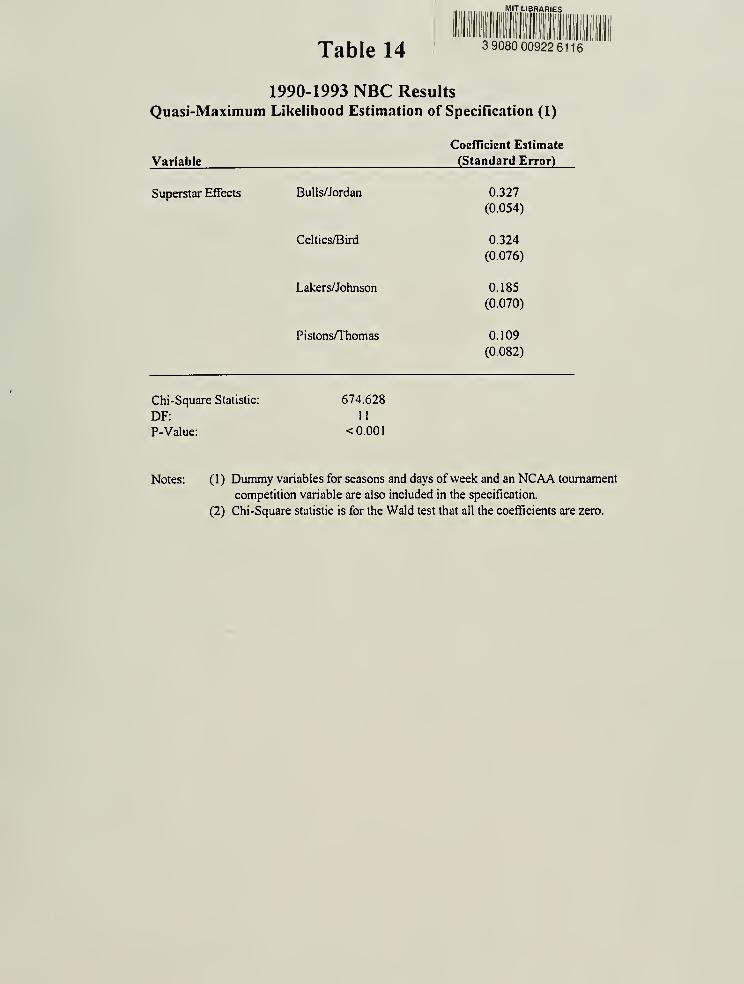
Table 14
MIT LIBRARIES
3 9080 00922 6116
1990-1993 NBC Results
Quasi-Maximum Likelihood Estimation of Specification (1)
Coefficient Estimate
Variable (Standard Error)
Superstar Effects Bulls/Jordan 0.327
(0.054)
Celtics/Bird 0.324
(0.076)
Lakers/Johnson 0.185
(0.070)
Pistons/Thomas 0.109
(0.082)
Chi-Square Statistic: 674.628
DF: 11
P-Value: < 0.001
Notes: (1) Dummy variables for seasons and days ofweek and an NCAA tournament
competition variable are also included in the specification.
(2) Chi-Square statistic is for the Wald test that all the coefficients are zero.
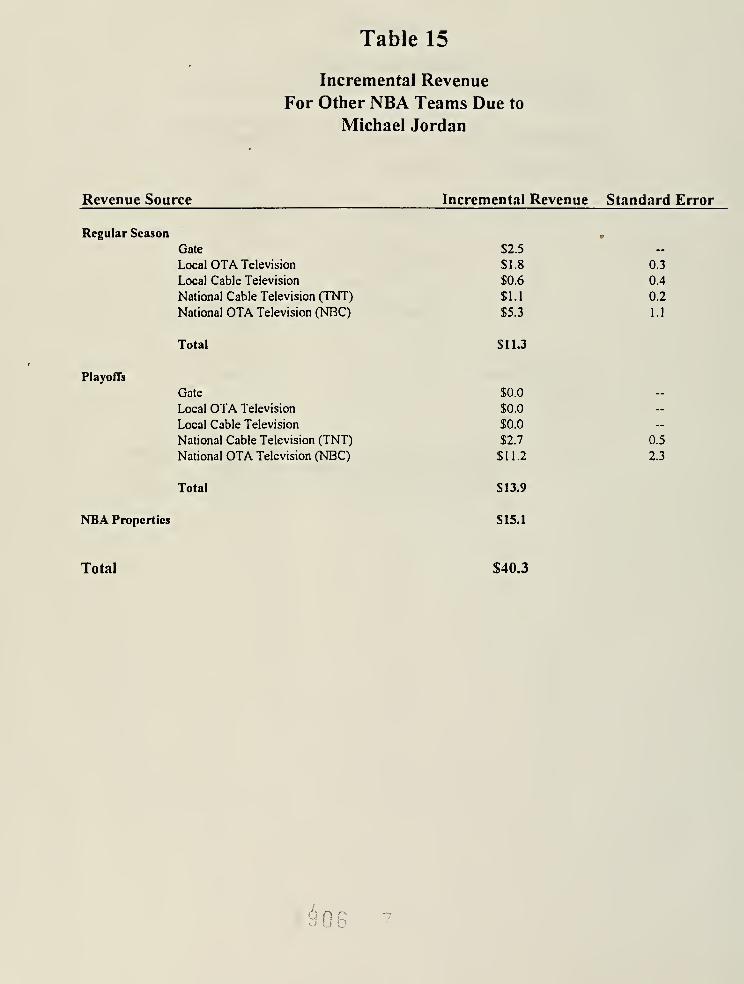
Table 15
Incremental Revenue
For Other NBA Teams Due to
Michael Jordan
Revenue Source Incremental Revenue Standard Error
Regular Season
Gate
Local OTA Television
Local Cable Television
National Cable Television (TNT)
National OTA Television (NBC)
$2.5
$1.8
$0.6
$1.1
$5.3
0.3
0.4
0.2
1.1
Total SI 1.3
Playoffs
Gate
Local OTA Television
Local Cable Television
National Cable Television (TNT)
National OTA Television (NBC)
$0.0
$0.0
$0.0
$2.7
$11.2
0.5
2.3
Total SI 3.9
NBA Properties S15.1
Total $40.3


Date Due
":'
DUE FtB 1i 1999
Lib-26-67


