Atmos. Chem. Phys., 11, 12217–12226, 2011www.atmos-chem-phys.net/11/12217/2011/doi:10.5194/acp-11-12217-2011© Author(s) 2011. CC Attribution 3.0 License.
AtmosphericChemistry
and Physics
Stratospheric ozone chemistry in the Antarctic: what determines thelowest ozone values reached and their recovery?
J.-U. Grooß1, K. Brautzsch1, R. Pommrich1,2,3, S. Solomon4, and R. Muller1
1Institut fur Energie- und Klimaforschung – Stratosphare (IEK-7), Forschungszentrum Julich, Julich, Germany2Laboratoire d’Aerologie, CNRS/INSU, Universite de Toulouse, Toulouse, France3Groupe d’etude de l’Atmosphere Meteorologique, CNRM-GAME, Meteo-France, Toulouse, France4Department of Atmospheric and Oceanic Science, University of Colorado, Boulder, CO, USA
Received: 27 July 2011 – Published in Atmos. Chem. Phys. Discuss.: 5 August 2011Revised: 18 November 2011 – Accepted: 25 November 2011 – Published: 7 December 2011
Abstract. Balloon-borne observations of ozone from theSouth Pole Station have been reported to reach ozone mix-ing ratios below the detection limit of about 10 ppbv at the70 hPa level by late September. After reaching a minimum,ozone mixing ratios increase to above 1 ppmv on the 70 hPalevel by late December. While the basic mechanisms caus-ing the ozone hole have been known for more than 20 yr, thedetailed chemical processes determining how low the localconcentration can fall, and how it recovers from the mini-mum have not been explored so far. Both of these aspectsare investigated here by analysing results from the ChemicalLagrangian Model of the Stratosphere (CLaMS). As ozonefalls below about 0.5 ppmv, a balance is maintained by gasphase production of both HCl and HOCl followed by het-erogeneous reaction between these two compounds in thesesimulations. Thereafter, a very rapid, irreversible chlorinedeactivation into HCl can occur, either when ozone drops tovalues low enough for gas phase HCl production to exceedchlorine activation processes or when temperatures increaseabove the polar stratospheric cloud (PSC) threshold. As aconsequence, the timing and mixing ratio of the minimumozone depends sensitively on model parameters, includingthe ozone initialisation. The subsequent ozone increase be-tween October and December is linked mainly to photochem-ical ozone production, caused by oxygen photolysis and bythe oxidation of carbon monoxide and methane.
Correspondence to:J.-U. Grooß([email protected])
1 Introduction
Since the discovery of the ozone hole (Farman et al., 1985),the chemical mechanisms causing ozone depletion have beenclarified in increasing detail (e.g.,Solomon, 1999; WMO,2011). These mechanisms lead to an almost complete de-struction of ozone at certain altitudes (≈15–20 km) in theAntarctic stratosphere, as observed in measurements byozone sondes over four decades (Solomon et al., 2005). Fig-ure1 shows the ozone observations from the South Pole Sta-tion at the 70 hPa level. The logarithmic ordinate highlightsthe massive loss of ozone at this level, with ozone mixingratios dropping to and even below the approximate instru-ment detection limit of 10 ppbv (seeVomel and Diaz, 2010)by late September and early October above the South PoleStation. There are some observations that do not displayozone depletion over the South Pole Station, e.g. betweenlate September and early November. These data correspondto times when the polar vortex was not located over the pole,particularly in 2002.
The graph reveals a lower envelope of the observations thathas remained nearly the same in different years since 1990,characterising the chemical decay of ozone to values as lowas 10 ppbv around the end of September and increasing againafterwards. While the basic mechanisms for the rapid polarozone loss are understood (Solomon, 1999), the explanationfor the ozone depletion near and below the detection limit ofabout 10 ppbv have not yet been elucidated, nor has the fac-tor driving the subsequent increase of ozone been identified.Here we use simulations of the Chemical Lagrangian Modelof the Stratosphere (CLaMS) to investigate these processes.
Published by Copernicus Publications on behalf of the European Geosciences Union.

12218 J.-U. Grooß et al.: Stratospheric ozone chemistry at lowest ozone values
South Pole Ozone at 70 hPa
Jul 1 Sep 1 Nov 1 Jan 110−9
10−8
10−7
10−6
Ozo
ne M
ixin
g R
atio
1990−1999 2000−2004 2005−2010
Fig. 1. Ozone sonde observations at 70 hPa from South Pole Stationin winter and spring since 1990. Updated from Fig. 7a ofSolomonet al.(2005).
2 Model description
The simulations presented here are performed with CLaMS(McKenna et al., 2002a,b; Konopka et al., 2004; Grooß et al.,2005a). The model is used in two different modes. In thebox-model mode, stratospheric chemistry is calculated for afew representative air parcels along their trajectory whereasthe global mode is the Lagrangian 3-dimensional ChemistryTransport Model.
In the box-model mode, the air parcels are defined hereby the location and time of ozone soundings in the ozonehole period, from which trajectories are calculated both back-ward to June and forward to December. Simulations withthe CLaMS chemistry module are then performed forwardin time using the combination of these two trajectories. Thetrajectories of the air parcels were calculated using wind andtemperature data from the ECMWF operational analysis in a1◦
×1◦ resolution. The diabatic descent (or ascent) rates werecalculated from a radiation code (Morcrette, 1991; Zhongand Haigh, 1995) for a cloud-free atmosphere based on tem-peratures from the ECMWF operational analyses and clima-tological ozone and water vapour profiles (Grooß and Rus-sell, 2005). CLaMS includes options for different solversto integrate the system of stiff ordinary differential equationsdescribing the chemistry (Carver et al., 1997; McKenna et al.,2002b). The chemical kinetic data are taken fromSanderet al. (2006), except for the Cl2O2 cross sections which aretaken fromvon Hobe et al.(2009), scaled by a factor of 1.48to match the observation ofLien et al.(2009). The photolysisrates are calculated in spherical geometry (Meier et al., 1982;Becker et al., 2000) for every hour using a climatologicalozone profile for ozone hole conditions from HALOE mea-surements (Grooß and Russell, 2005). Heterogeneous chem-istry is calculated on ice, nitric acid trihydrate (NAT), andliquid ternary H2O/H2SO4/HNO3 particles. The parametri-sations of the temperature-dependent uptake coefficient on
liquid aerosols are derived from measurements byHanson(1998) and those on NAT particles are taken fromCarslawand Peter(1997) based on lab measurements derived fromHanson and Ravishankara(1993). NAT formation is as-sumed to occur at a HNO3 supersaturation of a factor of10, corresponding approximately to 3 K supercooling belowTNAT . The NAT particle density is assumed to be 1 cm−3.
In the box-model mode, we employ the solver SVODE(Brown et al., 1989) that does not use the family approxima-tion, which could become invalid at very low ozone mixingratios. Since no denitrification parametrisation was used inthe box-model mode, the chemical consequences of the den-itrification were addressed by sensitivity studies. The chem-ical initialisation for the air parcels in the box-model modeis interpolated from the 3-dimensional CLaMS simulationsdescribed below. The results from box-model studies do notinclude mixing between neighbouring air masses nor denitri-fication due to sedimentation of HNO3-containing particles.Over the long time span from June to November, a trajectoryshould certainly not be viewed as representing the exact lo-cation of a single air mass. Rather it should be interpretedas one of the possible histories of an air parcel that reacheslow ozone mixing ratios. Thus, the results of this trajectory-box-model can be used to investigate the chemical processesaround the observed minimum ozone mixing ratios.
The CLaMS 3-D simulations for the ozone hole in the year2003 were described in detail in a dissertation for a univer-sity diploma (Walter, 2005), which focused on the time pe-riod up to November 2003. These simulations are continueduntil the end of December in this work. The CLaMS sim-ulations were initialised on 1 May 2003 using observationsfrom MIPAS-Envisat data for O3, N2O, and HNO3. Corre-lations with N2O were used to initialise Cly (Grooß et al.,2002), Bry (Grooß et al., 2002)+10 %, and NOy Grooß et al.(2005b). The remaining species and the family partitioningwere initialised from the Mainz 2-D model (Grooß, 1996).Denitrification by sedimenting NAT particles was simulatedwith the scheme used for the Arctic winter 2002/2003 (Grooßet al., 2005b). The horizontal resolution of this simulation is100 km between 40 and 90◦ S. Here, the solver IMPACT wasused based on the family concept approximation (Carver andScott, 2000).
3 Results
For investigations of the chemical processes around theozone minimum in late September, a trajectory was chosenthat exactly intersects an observation from the South PoleStation of about 10 ppbv ozone at the pressure level of 70 hPaon 24 September 2003. The box-model simulation was per-formed along this trajectory for the time period from 1 Juneto 30 November 2003. The trajectory stays in the vortex coreat an average equivalent latitude of 77◦ S with a standard de-viation of 5◦. This trajectory should be considered as an
Atmos. Chem. Phys., 11, 12217–12226, 2011 www.atmos-chem-phys.net/11/12217/2011/

J.-U. Grooß et al.: Stratospheric ozone chemistry at lowest ozone values 12219
390
400
410
420
430
θ [K
]
aPotential Temperature Trajectory Sonde
170180190200210220230
Tem
p. [K
]
b
0.01
0.10
1.00
O3
[ppm
v]
c
O3 (box model) O3 (Sonde)
0
2
4
6
Sur
face
[μm
2 /cm
3 ]
d A(NAT) A(liquid)
0.00.51.01.52.02.53.0
HC
l, C
lOx
[ppb
v]
eHCl ClOX HOCl
0.01
0.10
1.00
10.00
Rat
e [p
pbv/
d]
f
Cl activation rate Cl deactivation rate
Jul 1 Sep 1 Nov 1
0.1
1.0
10.0
100.0
Rat
e [p
pbv/
d]
g Cl2O2+hν BrO+ClO HOCl+hν P(O3)
Fig. 2. Box-model simulations along a trajectory passing throughthe location of the ozone sonde observation of 10 ppbv on 73 hPa on24 September 2003. The different panels show a time series of therelevant parameters:(a) potential temperature of the air parcel,(b)temperature,(c) ozone (red),(d) surface area density of NAT andliquid aerosol,(e)ClOx, ClONO2 and HCl,(f) net rates of chlorineactivation and deactivation,(g) rates of catalytic cycles involvingozone including ozone production rate by O2+hν (black solid line)and total ozone production rate (black dotted line). For reasons ofclarity, the reaction rates(f, g) are plotted as 24 h running averages.
example of the possible development for which the chemistryis investigated in detail. Figure2 shows the development ofthe relevant chemical species and reaction rates along the tra-jectory. Panel a shows the potential temperature of the airparcel with the typical diabatic descent in the polar vortexand panel b shows the temperature along the trajectory. Inpanel c we show the simulated ozone mixing ratio. The cho-sen ozone sonde observation used to determine the trajectoryis plotted as a black star symbol. The simulation does reach
Fig. 3. Schematic of the primary chlorine activation and deacti-vation reactions occurring in mid-September in these simulations.
ozone mixing ratios as low as those observed, but a a timeseveral days after the ozone sonde observation of 10 ppbv.
3.1 Chlorine deactivation and heterogeneous chemistry
We first focus on the time period of two weeks before thesimulated ozone minimum (grey shaded area in Fig.2). Thesimulation shows that the cessation of ozone loss (yieldinga minimum near 10 ppbv) is caused by a very fast deactiva-tion of active chlorine compounds into the reservoir speciesHCl on a very short time scale of about a day. Althoughthe temperatures are still low enough for the existence ofpolar stratospheric clouds (PSCs), chlorine activation doesnot occur after the ozone minimum because practically allof the inorganic chlorine is in the form of HCl so that nei-ther ClONO2 nor HOCl are available as reaction partnersfor HCl in heterogeneous chlorine activation processes. Fig-ure3 shows a simplified schematic of the primary pathwaysof chlorine activation and chlorine deactivation. The pho-tochemical equilibrium between Cl and ClO is indicated bythick black arrows. The main heterogeneous chlorine acti-vation reaction during the period shown by the grey shad-ing is HOCl+HCl, which produces Cl2. Photolysis of Cl2then produces ClOx (=Cl+ClO+2×Cl2O2). A similar cycleis also possible through the formation of ClONO2 insteadof HOCl, which is, however, not more than about 0.1 % asfast at this time in the simulation for ozone mixing rationsbelow 0.5 ppmv. The chlorine deactivation into HCl occursthrough the reactions Cl+CH4 and Cl+CH2O. HOCl is be-ing formed mainly by the reaction ClO+HO2 (rather thanby heterogeneous reaction of ClONO2 with H2O) in thissimulation, and it is decomposed by photolysis as well asthrough heterogeneous reactions. This chain stops if all chlo-rine compounds are deactivated into HCl. The fast chlorine
www.atmos-chem-phys.net/11/12217/2011/ Atmos. Chem. Phys., 11, 12217–12226, 2011
12220 J.-U. Grooß et al.: Stratospheric ozone chemistry at lowest ozone values
deactivation into the reservoir HCl can be elucidated by look-ing at the net chlorine activation and deactivation rates thatare shown in panel f of Fig.2. The blue line corresponds tothe sum of all activation reactions that decompose HCl (orClONO2), mainly the heterogeneous reaction of HOCl+HCl.The red line corresponds to the sum of all deactivation reac-tions in which HCl or ClONO2 are formed, mainly Cl+CH4,Cl+CH2O. It is apparent that the chlorine activation and de-activation rates are approximately balanced and they increaseto values of the order of 10 ppbv per day in the period beforethe ozone minimum. This deactivation rate would lead toa complete chlorine deactivation within about 6 h if hetero-geneous chlorine activation did not occur at the same time.The chlorine activation rate in late October and Novemberis mainly due to the gas phase reaction of HCl+OH andClONO2 photolysis.
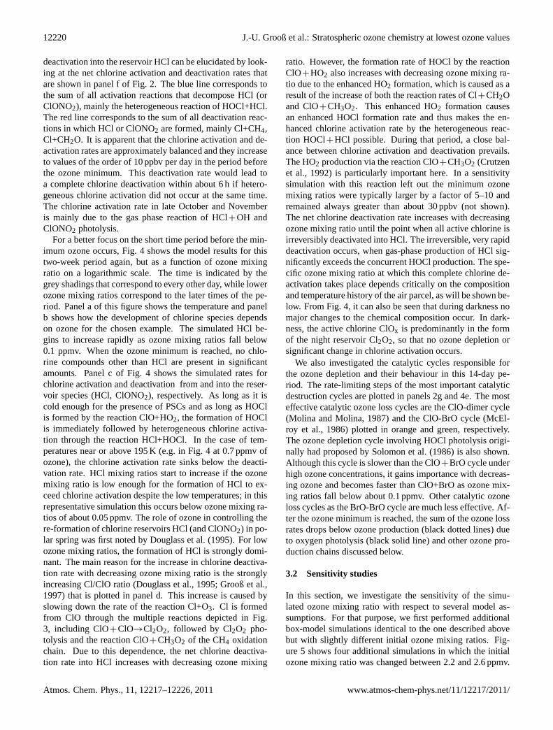
For a better focus on the short time period before the min-imum ozone occurs, Fig.4 shows the model results for thistwo-week period again, but as a function of ozone mixingratio on a logarithmic scale. The time is indicated by thegrey shadings that correspond to every other day, while lowerozone mixing ratios correspond to the later times of the pe-riod. Panel a of this figure shows the temperature and panelb shows how the development of chlorine species dependson ozone for the chosen example. The simulated HCl be-gins to increase rapidly as ozone mixing ratios fall below0.1 ppmv. When the ozone minimum is reached, no chlo-rine compounds other than HCl are present in significantamounts. Panel c of Fig.4 shows the simulated rates forchlorine activation and deactivation from and into the reser-voir species (HCl, ClONO2), respectively. As long as it iscold enough for the presence of PSCs and as long as HOClis formed by the reaction ClO+HO2, the formation of HOClis immediately followed by heterogeneous chlorine activa-tion through the reaction HCl+HOCl. In the case of tem-peratures near or above 195 K (e.g. in Fig.4 at 0.7 ppmv ofozone), the chlorine activation rate sinks below the deacti-vation rate. HCl mixing ratios start to increase if the ozonemixing ratio is low enough for the formation of HCl to ex-ceed chlorine activation despite the low temperatures; in thisrepresentative simulation this occurs below ozone mixing ra-tios of about 0.05 ppmv. The role of ozone in controlling there-formation of chlorine reservoirs HCl (and ClONO2) in po-lar spring was first noted byDouglass et al.(1995). For lowozone mixing ratios, the formation of HCl is strongly domi-nant. The main reason for the increase in chlorine deactiva-tion rate with decreasing ozone mixing ratio is the stronglyincreasing Cl/ClO ratio (Douglass et al., 1995; Grooß et al.,1997) that is plotted in panel d. This increase is caused byslowing down the rate of the reaction Cl+O3. Cl is formedfrom ClO through the multiple reactions depicted in Fig.3, including ClO+ClO→Cl2O2, followed by Cl2O2 pho-tolysis and the reaction ClO+CH3O2 of the CH4 oxidationchain. Due to this dependence, the net chlorine deactiva-tion rate into HCl increases with decreasing ozone mixing
ratio. However, the formation rate of HOCl by the reactionClO+HO2 also increases with decreasing ozone mixing ra-tio due to the enhanced HO2 formation, which is caused as aresult of the increase of both the reaction rates of Cl+CH2Oand ClO+CH3O2. This enhanced HO2 formation causesan enhanced HOCl formation rate and thus makes the en-hanced chlorine activation rate by the heterogeneous reac-tion HOCl+HCl possible. During that period, a close bal-ance between chlorine activation and deactivation prevails.The HO2 production via the reaction ClO+CH3O2 (Crutzenet al., 1992) is particularly important here. In a sensitivitysimulation with this reaction left out the minimum ozonemixing ratios were typically larger by a factor of 5–10 andremained always greater than about 30 ppbv (not shown).The net chlorine deactivation rate increases with decreasingozone mixing ratio until the point when all active chlorine isirreversibly deactivated into HCl. The irreversible, very rapiddeactivation occurs, when gas-phase production of HCl sig-nificantly exceeds the concurrent HOCl production. The spe-cific ozone mixing ratio at which this complete chlorine de-activation takes place depends critically on the compositionand temperature history of the air parcel, as will be shown be-low. From Fig.4, it can also be seen that during darkness nomajor changes to the chemical composition occur. In dark-ness, the active chlorine ClOx is predominantly in the formof the night reservoir Cl2O2, so that no ozone depletion orsignificant change in chlorine activation occurs.
We also investigated the catalytic cycles responsible forthe ozone depletion and their behaviour in this 14-day pe-riod. The rate-limiting steps of the most important catalyticdestruction cycles are plotted in panels2g and4e. The mosteffective catalytic ozone loss cycles are the ClO-dimer cycle(Molina and Molina, 1987) and the ClO-BrO cycle (McEl-roy et al., 1986) plotted in orange and green, respectively.The ozone depletion cycle involving HOCl photolysis origi-nally had proposed bySolomon et al.(1986) is also shown.Although this cycle is slower than the ClO+BrO cycle underhigh ozone concentrations, it gains importance with decreas-ing ozone and becomes faster than ClO+BrO as ozone mix-ing ratios fall below about 0.1 ppmv. Other catalytic ozoneloss cycles as the BrO-BrO cycle are much less effective. Af-ter the ozone minimum is reached, the sum of the ozone lossrates drops below ozone production (black dotted lines) dueto oxygen photolysis (black solid line) and other ozone pro-duction chains discussed below.
3.2 Sensitivity studies
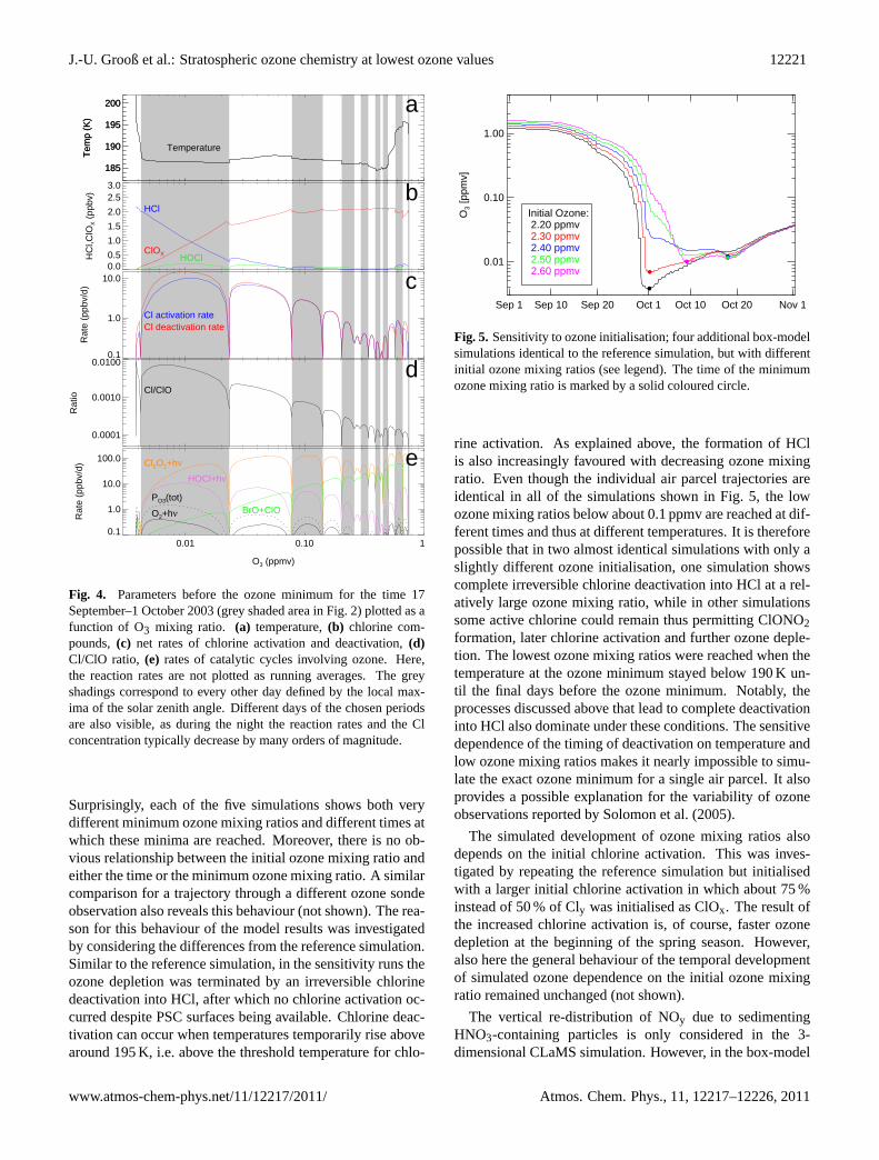
In this section, we investigate the sensitivity of the simu-lated ozone mixing ratio with respect to several model as-sumptions. For that purpose, we first performed additionalbox-model simulations identical to the one described abovebut with slightly different initial ozone mixing ratios. Fig-ure 5 shows four additional simulations in which the initialozone mixing ratio was changed between 2.2 and 2.6 ppmv.
Atmos. Chem. Phys., 11, 12217–12226, 2011 www.atmos-chem-phys.net/11/12217/2011/
J.-U. Grooß et al.: Stratospheric ozone chemistry at lowest ozone values 12221
185
190
195
200
Tem
p (K
)
Temperature
a
185
190
195
200
Tem
p (K
)
0.00.5
1.0
1.5
2.0
2.53.0
HC
l,ClO
X (
ppbv
)
HCl
ClOX HOCl
b
0.1
1.0
10.0
Rat
e (p
pbv/
d)
Cl activation rateCl deactivation rate
c
0.0001
0.0010
0.0100
Rat
io
Cl/ClO
d
0.01 0.10 1
O3 (ppmv)
0.1
1.0
10.0
100.0
Rat
e (p
pbv/
d) Cl2O2+hν
BrO+ClOO2+hν
HOCl+hν
PO3(tot)
e
Fig. 4. Parameters before the ozone minimum for the time 17September–1 October 2003 (grey shaded area in Fig.2) plotted as afunction of O3 mixing ratio. (a) temperature,(b) chlorine com-pounds,(c) net rates of chlorine activation and deactivation,(d)Cl/ClO ratio, (e) rates of catalytic cycles involving ozone. Here,the reaction rates are not plotted as running averages. The greyshadings correspond to every other day defined by the local max-ima of the solar zenith angle. Different days of the chosen periodsare also visible, as during the night the reaction rates and the Clconcentration typically decrease by many orders of magnitude.
Surprisingly, each of the five simulations shows both verydifferent minimum ozone mixing ratios and different times atwhich these minima are reached. Moreover, there is no ob-vious relationship between the initial ozone mixing ratio andeither the time or the minimum ozone mixing ratio. A similarcomparison for a trajectory through a different ozone sondeobservation also reveals this behaviour (not shown). The rea-son for this behaviour of the model results was investigatedby considering the differences from the reference simulation.Similar to the reference simulation, in the sensitivity runs theozone depletion was terminated by an irreversible chlorinedeactivation into HCl, after which no chlorine activation oc-curred despite PSC surfaces being available. Chlorine deac-tivation can occur when temperatures temporarily rise abovearound 195 K, i.e. above the threshold temperature for chlo-
Sep 1 Sep 10 Sep 20 Oct 1 Oct 10 Oct 20 Nov 1
0.01
0.10
1.00
O3
[ppm
v]
Initial Ozone: 2.20 ppmv 2.30 ppmv 2.40 ppmv 2.50 ppmv 2.60 ppmv
Fig. 5. Sensitivity to ozone initialisation; four additional box-modelsimulations identical to the reference simulation, but with differentinitial ozone mixing ratios (see legend). The time of the minimumozone mixing ratio is marked by a solid coloured circle.
rine activation. As explained above, the formation of HClis also increasingly favoured with decreasing ozone mixingratio. Even though the individual air parcel trajectories areidentical in all of the simulations shown in Fig.5, the lowozone mixing ratios below about 0.1 ppmv are reached at dif-ferent times and thus at different temperatures. It is thereforepossible that in two almost identical simulations with only aslightly different ozone initialisation, one simulation showscomplete irreversible chlorine deactivation into HCl at a rel-atively large ozone mixing ratio, while in other simulationssome active chlorine could remain thus permitting ClONO2formation, later chlorine activation and further ozone deple-tion. The lowest ozone mixing ratios were reached when thetemperature at the ozone minimum stayed below 190 K un-til the final days before the ozone minimum. Notably, theprocesses discussed above that lead to complete deactivationinto HCl also dominate under these conditions. The sensitivedependence of the timing of deactivation on temperature andlow ozone mixing ratios makes it nearly impossible to simu-late the exact ozone minimum for a single air parcel. It alsoprovides a possible explanation for the variability of ozoneobservations reported bySolomon et al.(2005).
The simulated development of ozone mixing ratios alsodepends on the initial chlorine activation. This was inves-tigated by repeating the reference simulation but initialisedwith a larger initial chlorine activation in which about 75 %instead of 50 % of Cly was initialised as ClOx. The result ofthe increased chlorine activation is, of course, faster ozonedepletion at the beginning of the spring season. However,also here the general behaviour of the temporal developmentof simulated ozone dependence on the initial ozone mixingratio remained unchanged (not shown).
The vertical re-distribution of NOy due to sedimentingHNO3-containing particles is only considered in the 3-dimensional CLaMS simulation. However, in the box-model
www.atmos-chem-phys.net/11/12217/2011/ Atmos. Chem. Phys., 11, 12217–12226, 2011

12222 J.-U. Grooß et al.: Stratospheric ozone chemistry at lowest ozone values
simulation it is possible to include denitrification by remov-ing HNO3 from the model when NAT is present by a simpleparametrisation (Grooß et al., 2002). This parametrisationwas used here to study the sensitivity of the results with re-spect to denitrification. The denitrification was adjusted suchthat about 3 ppbv of HNO3 remained in the box in November,consistent with ACE-FTS observations (Jones et al., 2011b).Individual simulations look different when the denitrificationis included and all other model parameters remain identical.However, in general in the case of increased denitrification,the minimum ozone mixing ratio is somewhat larger and itis reached at a later time. This can be explained by two ef-fects. First, a slightly lower chlorine activation, which is dueto less NO2 being available, which makes the formation ofClONO2 slower and thus decreases the heterogeneous acti-vation through ClONO2+HCl. Second, less HNO3 causessmaller surfaces of solid and liquid PSCs, which slows downthe heterogeneous chlorine activation reactions. With thedenitrification parametrisation, the maximum of the chlorinedeactivation rate is about 50 % lower than for the referencesimulation. However, also here the general behaviour of thetemporal development of simulated ozone dependence on theinitial ozone mixing ratio remained unchanged (not shown).Denitrification also causes a slower rate of increase in ozoneafter the minimum, as will be discussed below.
3.3 Ozone recovery
From the ozone sonde measurements at the South Pole (Fig.1), it is evident that after early October the lower envelopeof the ozone observations increases again with time. Possi-ble explanations for this increase are either in situ productionof ozone or mixing with air masses containing larger ozonemixing ratios. However, the increase occurs smoothly, sug-gesting a likely role for chemistry rather than mixing alone,which would be expected to be episodic and variable. Inthe box-model results, the in situ chemical ozone produc-tion can be probed. To investigate the latitude and altitudedependence of the in situ ozone production, multiple box-model simulations were performed along artificial trajecto-ries in which latitude, temperature and pressure level werekept constant over the period from October to December.
These simulations were initialised assuming completechlorine deactivation (HCl = Cly), 1 ppbv ozone, and4.5 ppbv NOy corresponding to moderate denitrification. Theanalysis of these simulations shows that three reaction chainsare responsible for the ozone production. One of these isthe well-known production by oxygen photolysis (Chapman,1930).
O2+hν → 2O
O+O2+M → O3 (2×)
3O2 → 2O3 (R1)
Two other reaction chains make important contributions tothe modelled ozone production, namely the oxidation of COand CH4.
CO+OH → H +CO2
H+O2+M → HO2
HO2+NO → NO2+OH
NO2+hν → NO+O
O+O2+M → O3
CO+2O2 → CO2+O3 (R2)
and
CH4+Cl → CH3+HCl
HCl+OH → Cl+H2O
CH3+O2+M → CH3OO
CH3OO+NO → NO2+CH2O+H
H+O2+M → HO2
HO2+NO → NO2+OH
NO2+hν → NO+O (2×)
O+O2+M → O3 (2×)
CH4+4O2 → CH2O+H2O+2O3 (R3)
Alternatively, when replaced by the following reaction, thefirst 2 reactions of Reaction ChainR3 result in a chain withthe same sum reaction.
CH4+OH → CH3+H2O (R4)
A further minor ozone production chain is also initiatedby the oxidation of CH2O, which is not considered in detailhere. In each of the above reaction chains, the slowest re-action that determines the ozone production rate is writtenin bold face. (Note that in the presence of PSCs and activechlorine the heterogeneous reaction HOCl+HCl occurs inparallel to HCl+OH in Reaction ChainR3. In that case,the reaction CH3OO+NO determines the rate of ReactionsChainsR3 andR4). For typical stratospheric ozone mixingratios, the ozone production rates of Reaction ChainsR2 toR4are of the order of 1 ppbv per day and therefore relativelyunimportant. These cycles dominate ozone production heredue to the low solar elevation. Figure6 shows the simulatedozone increase between 1 October and 30 November for thethree pressure levels 100, 70, and 50 hPa. The dashed linecorresponds to the ozone increase due to oxygen photolysisonly (Reaction ChainR1). The dotted lines correspond to thesum of the rates limiting Reactions Chains R1 to R4 includ-ing oxygen photolysis. It is slightly larger than the calculatednet ozone production (solid lines), because some ozone de-pletion cycles also occur (see also Fig.2g).
Atmos. Chem. Phys., 11, 12217–12226, 2011 www.atmos-chem-phys.net/11/12217/2011/

J.-U. Grooß et al.: Stratospheric ozone chemistry at lowest ozone values 12223
0 50 100 150 200 250
Ozone increase Oct/Nov [ppbv]
−90
−85
−80
−75
−70
−65
−60La
titud
e [d
egre
es]
Pressure 100 hPa 70 hPa 50 hPa
Fig. 6. Simulated ozone increase between 1 October and 30 Novem-ber as a function of latitude for three pressure levels using overheadozone profile from climatology. Solid lines indicate the simulatedozone increase, dashed lines show the ozone increase due to oxy-gen photolysis (Reaction ChainR1). Dotted lines show the sum ofozone production by reaction chains 1 to 4.
In Figs. 2g and4e, the dotted black lines correspond tothe ozone production rate due to the sum of all ozone pro-duction chains (Reaction Chains R1 to R4). This part of theozone production increases with increasing altitude. It alsoincreases with distance from the South Pole due to the in-creasing solar elevation. The fraction of ozone productioncaused by the CO and CH4 oxidation (Reaction ChainsR2toR4) corresponds to the difference between the dotted and thedashed line. It remains approximately constant with altitudeand latitude.
For the results shown in Fig.6, the oxygen photolysis ratewas calculated using a climatological overhead ozone pro-file (Grooß and Russell, 2005) that contains average ozonemixing ratios for the ozone hole time period. However, it ispossible that the ozone profile above the observations show-ing very low ozone mixing ratio at the lower envelope mayalso be significantly below average. This would cause anincrease in the oxygen photolysis rate and therefore in theozone production rate. To investigate this sensitivity, we re-peated the simulations assuming a reduced overhead ozoneprofile. The ozone profile was reduced by a factor of 5 be-tween 30 and 150 hPa south of 65◦ S. The results obtainedwith this reduced overhead ozone profile are displayed inFig. 7. A larger ozone production is evident, especially at the50 hPa level towards the vortex edge. However, air masseswith ozone mixing ratios well below average may not remainvertically aligned over a period of two months.
The ozone production rate due to Reaction Chains (R2)and (R3) depends on the available active nitrogen(NOx=NO+NO2) and is strongly influenced by denitrifica-tion. A decrease in NOy also implies a decrease in NOx. TheNOx dependence of ozone production rates was already in-vestigated in the context of evaluating the impact of aircraft
0 100 200 300 400
Ozone increase Oct/Nov [ppbv]
−90
−85
−80
−75
−70
−65
−60
Latit
ude
[deg
rees
]
Pressure 100 hPa 70 hPa 50 hPa
Fig. 7. As Fig.6, but using an overhead ozone profile reduced by afactor of 5 between 30 and 150 hPa.
p=70hPa, sensitivity NOy
0 20 40 60 80 100 120 140
Ozone increase Oct/Nov [ppbv]
−90
−85
−80
−75
−70
−65
−60
Latit
ude
[deg
rees
]
NOy [ppbv] 2.5 3.5 4.5 6.0 8.0
Fig. 8. Simulated ozone increase between 1 October and 30 Novem-ber for the 70 hPa level (blue line in Fig.6) for different values ofNOy. The ozone increase due to oxygen photolysis (dashed line) isthe same for all simulations.
emissions on the chemical composition of the tropopause re-gion (e.g., Grooß et al., 1998). Figure8 shows the sensi-tivity of ozone production with respect to NOy (ranging be-tween 2.5 and 8 ppbv) for the simulation on the 70 hPa level.Figure 8 shows that the ozone increase is slower for moredenitrified air. This demonstrates the importance of ozoneproduction due to CO and CH4 oxidation. An increase inNOx increases the Cl/ClO ratio due to the faster NO+ClO re-action and a larger OH/HO2 ratio due to the faster NO+HO2reaction.
For comparison with the range of observed ozone obser-vations, we now show sensitivity simulations for realistictrajectories that include diabatic descent and latitude varia-tions. The box-model simulations of the same kind as shownin Sect. 3.1 were initialised on 1 August interpolated fromthe 3-dimensional CLaMS CTM simulation.
www.atmos-chem-phys.net/11/12217/2011/ Atmos. Chem. Phys., 11, 12217–12226, 2011

12224 J.-U. Grooß et al.: Stratospheric ozone chemistry at lowest ozone values
South Pole Ozone at θ=375 K
Aug 1 Sep 1 Oct 1 Nov 1 Dec 1
10−8
10−7
10−6
Ozo
ne [p
pmv]
1990−1999 2000−2004 2005−2010 CLaMS−3D min
South Pole Ozone at θ=400 K
Aug 1 Sep 1 Oct 1 Nov 1 Dec 1
10−8
10−7
10−6
Ozo
ne [p
pmv]
1990−1999 2000−2004 2005−2010 CLaMS−3D min
South Pole Ozone at θ=450 K
Aug 1 Sep 1 Oct 1 Nov 1 Dec 1
10−8
10−7
10−6
Ozo
ne [p
pmv]
1990−1999 2000−2004 2005−2010 CLaMS−3D min
South Pole Ozone at θ=500 K
Aug 1 Sep 1 Oct 1 Nov 1 Dec 1
10−8
10−7
10−6
Ozo
ne [p
pmv]
1990−1999 2000−2004 2005−2010 CLaMS−3D min
Fig. 9. Comparison of South Pole ozone observations with box-model simulations for 4 different levels. The vertical coordinate is potentialtemperature. South Pole observations for different yeas are plotted as grey symbols. CLaMS box-model simulations are shown for 21trajectories per level that pass the South Pole on this level at different times in 2003 (red: 20–26 September; green: 27 September–3 October;blue: 4–10 October). For trajectories that reach latitudes north of 50◦ S, only the results up to this latitude are shown. The black linecorresponds to the minimum ozone mixing ratio of the CLaMS 3-D simulation poleward of 75◦ S equivalent latitude for the individuallevels.
To obtain realistic initial chlorine activation, the initialisa-tion of ClONO2 and HCl was taken from a climatology basedon ACE-FTS observations (Jones et al., 2011a). To avoidunrealistic denitrification, the lowest NOy and H2O mixingratios derived from the CLaMS 3-D simulation were not al-lowed to sink below 2.0 ppbv and 2.0 ppmv, respectively. Itis important to note that part of the ozone increase in Novem-ber and December on the 70 hPa level (Fig.1) is neither dueto photochemical ozone production nor mixing. It is causedby the typical climatological temperature increase in spring,which leads to an increase of potential temperature on a con-stant pressure level. The change in potential temperature at70 hPa between 1 October and 1 December is about 38 K.Since in spring the air masses remain on slowly descendingpotential temperature levels, the time series of observationson constant pressure levels in Fig.1 corresponds to differentaltitude origins. Therefore we compare the simulations withdata on potential temperature levels. Here, the box-modelsimulations were performed along trajectories that pass ex-actly over the South Pole on 21 days (20 September to 10October 2003) for each of the potential temperature levels
375 K, 400 K, 450 K, and 500 K. For the period between1 October and 1 December, the average diabatic descent forthe chosen trajectory for the lower three levels (375 K, 400 K,450 K) is below 10 K and 20 K for the 500 K level.
Although the latitude of trajectories changes with time, weargue that the simulated chemical ozone production shouldbe similar to the South Pole observations, because, to firstorder, similar ozone loss would be expected for an air par-cel starting at the pole and ending at latitudex comparedwith an air parcel starting at latitudex and ending at the polefor the same time period. This is because the noontime so-lar elevation increases from pole to mid-latitude, while thetime of solar hours per day increases from mid-latitude tothe pole. Further, the results of single box-model runs canonly be taken as an example, since the development of theresults very sensitively depends on the initial ozone mixingratio as shown in the previous sections. The simulated ozonemixing ratios for these simulations are shown in Fig.9. Gen-erally it can be seen that the simulations overlay the rangeof the observations. At the 375 K and 400 K levels, the sim-ulated ozone for many of the trajectories follows the lower
Atmos. Chem. Phys., 11, 12217–12226, 2011 www.atmos-chem-phys.net/11/12217/2011/

J.-U. Grooß et al.: Stratospheric ozone chemistry at lowest ozone values 12225
envelope of the ozone observations well. On the 500 K po-tential temperature level, the majority of the box-model sim-ulations have ozone mixing ratios below the lower envelopeof the observations. An important reason for the differenceat the 500 K level is diabatic descent. For example, the lowerenvelope of the South Pole observations on 1 December at480 K is around 340 ppbv while at 500 K it is 480 ppbv, im-plying that a 20K descent deplacement would be importantto the results. Generally, mixing of air masses which is notconsidered in the box-model simulations would also yield anincrease in ozone.
The minimum ozone mixing ratio between equivalent lat-itudes of 75◦ S and 90◦ S of the CLaMS 3-D simulation isplotted as a thick black line. In August at the lower levels of375 K and 400 K about 5 % and 1 % of the CLaMS air parcelsare below the envelope of the ozone sonde observations, re-spectively. This is most likely due to deficits in the ozoneinitialisation at the lower altitudes, which are, however, notimportant for the conclusions drawn here. The CLaMS 3-Dsimulation also fails to reach the minimum ozone mixing ra-tios that are seen in the observations, probably due to the lowresolution of the model simulation. On the 400 K and 450 Klevel, the increase in minimum ozone in October and Novem-ber in the 3-D simulation is faster than in the box-model sim-ulations. This additional increase can be explained by mix-ing, which is potentially overestimated in the 3-D CLaMSsimulation. However, from the results shown it is clear thatin situ ozone production by the reaction chains mentionedabove can explain much of the observed ozone increase inOctober and November.
4 Conclusions
In this paper, we have discussed several processes that areresponsible for Antarctic ozone depletion. We showed thatthe observed very low ozone mixing ratios in late Septem-ber and early October can be reproduced in box-model sim-ulations. A critical constraint on the minimum ozone thatcan be reached is fast irreversible chlorine deactivation intoHCl, which is triggered by very low ozone mixing ratiosand makes the ozone loss self-limiting. Ozone depletion cantherefore cease as ozone falls to very low values, even thoughsurfaces of solid and/or liquid PSCs are still present. Thetiming and the value of this minimum ozone mixing ratio arevery sensitive to different model parameters, in particular theinitial ozone mixing ratio, therefore it is not possible in allcases to exactly predict these parameters for a single air mass.The increase of the ozone mixing ratios after the minimum ismostly explained by in situ chemical ozone production bothby oxygen photolysis and as a consequence of methane andcarbon monoxide oxidation. An additional ozone increasecaused by mixing ond/or descent is also possible, particu-larly for later times in the spring season.
Acknowledgements.We thank Herman Smit and Peter von derGathen for helpful discussions on the detection limits of ozonesondes. This work was supported by the RECONCILE project ofthe European Commission Seventh Framework Programme (FP7)under the Grant number RECONCILE-226365-FP7-ENV-2008-1.
Edited by: D. Knopf
References
Becker, G., Grooß, J.-U., McKenna, D. S., and Muller, R.: Strato-spheric photolysis frequencies: Impact of an improved numericalsolution of the radiative transfer equation, J. Atmos. Chem., 37,217–229,doi:10.1023/A:1006468926530, 2000.
Brown, P. N., Byrne, G. D., and Hindmarsh, A. C.: VODE: A vari-able coefficient ODE solver, SIAM J. Sci. Stat. Comput., 10,1038–1051, 1989.
Carslaw, K. S. and Peter, T.: Uncertainties in reactive uptake co-efficients for solid stratospheric particles – 1. Surface chemistry,Geophys. Res. Lett., 24, 1743–1746, 1997.
Carver, G. D. and Scott, P. A.: IMPACT: an implicit time integra-tion scheme for chemical species and families, Ann. Geophys.,18, 337–346, 2000,http://www.ann-geophys.net/18/337/2000/.
Carver, G. D., Brown, P. D., and Wild, O.: The ASAD atmosphericchemistry integration package and chemical reaction database,Comput. Phys. Comm., 105, 197–215, 1997.
Chapman, S.: A theory of upper atmospheric ozone, Mem. Roy.Soc., 3, 103–109, 1930.
Crutzen, P. J., Muller, R., Bruhl, C., and Peter, T.: On the po-tential importance of the gas phase reaction CH3O2+ClO →
ClOO+CH3O and the heterogeneous reaction HOCl+HCl →H2O+Cl2 in “ozone hole” chemistry, Geophys. Res. Lett., 19,1113–1116,doi:10.1029/92GL01172, 1992.
Douglass, A. R., Schoeberl, M. R., Stolarski, R. S., Waters, J. W.,Russell III, J. M., Roche, A. E., and Massie, S. T.: Interhemi-spheric differences in springtime production of HCl and ClONO2in the polar vortices, J. Geophys. Res., 100, 13967–13978, 1995.
Farman, J. C., Gardiner, B. G., and Shanklin, J. D.: Large losses oftotal ozone in Antarctica reveal seasonal ClOx/NOx interaction,Nature, 315, 207–210, 1985.
Grooß, J.-U.: Modelling of Stratospheric Chemistry based onHALOE/UARS Satellite Data, PhD thesis, University of Mainz,Germany, 1996.
Grooß, J.-U. and Russell, J. M.: Technical note: A stratospheric cli-matology for O3, H2O, CH4, NOx, HCl, and HF derived fromHALOE measurements, Atmos. Chem. Phys., 5, 2797–2807,doi:10.5194/acp-5-2797-2005, 2005.
Grooß, J.-U., Pierce, R. B., Crutzen, P. J., Grose, W. L., and Rus-sell III, J. M.: Re-formation of chlorine reservoirs in southernhemisphere polar spring, J. Geophys. Res., 102, 13141–13152,doi:10.1029/96JD03505, 1997.
Grooß, J.-U., Bruhl, C., and Peter, T.: Impact of aircraft emissionson tropospheric and stratospheric ozone, I: Chemistry and 2-Dmodel results, Atmos. Environ., 32, 3173–3184, 1998.
Grooß, J.-U., Gunther, G., Konopka, P., Muller, R., McKenna,D. S., Stroh, F., Vogel, B., Engel, A., Muller, M., Hoppel, K.,Bevilacqua, R., Richard, E., Webster, C. R., Elkins, J. W., Hurst,D. F., Romashkin, P. A., and Baumgardner, D. G.: Simula-
www.atmos-chem-phys.net/11/12217/2011/ Atmos. Chem. Phys., 11, 12217–12226, 2011

12226 J.-U. Grooß et al.: Stratospheric ozone chemistry at lowest ozone values
tion of ozone depletion in spring 2000 with the Chemical La-grangian Model of the Stratosphere (CLaMS), J. Geophys. Res.,107, 8295,doi:10.1029/2001JD000456, 2002.
Grooß, J.-U., Konopka, P., and Muller, R.: Ozone chemistry dur-ing the 2002 Antarctic vortex split, J. Atmos. Sci., 62, 860–870,2005a.
Grooß, J.-U., Gunther, G., Muller, R., Konopka, P., Bausch, S.,Schlager, H., Voigt, C., Volk, C. M., and Toon, G. C.: Simulationof denitrification and ozone loss for the Arctic winter 2002/2003,Atmos. Chem. Phys., 5, 1437–1448,doi:10.5194/acp-5-1437-2005, 2005b.
Hanson, D. R.: Reaction of ClONO2 with H2O and HCl in sulfuricacid and HNO3/H2SO4/H2O mixtures, J. Phys. Chem. A, 102,4794–4807, 1998.
Hanson, D. R. and Ravishankara, A. R.: Reaction of ClONO2 withHCl on NAT, NAD, and frozen sulfuric acid and hydrolysis ofN2O5 and ClONO2 on frozen sulfuric acid, J. Geophys. Res.,98, 22931–22936, 1993.
Jones, A., Qin, G., Strong, K., Walker, K. A., McLinden, C.,M. Toohey, T., Kerzenmacher, Bernath, P., and Boone, C.: Aglobal inventory of stratospheric NOy from ACE-FTS, J. Geo-phys. Res., 116, D17304,doi:10.1029/2010JD015465, 2011a.
Jones, A., Walker, K. A., Jin, J. J., Taylor, J. R., Boone, C. D.,Bernath, P. F., Brohede, S., Manney, G. L., McLeod, S., Hughes,R., and Daffer, W. H.: Technical Note: A trace gas climatologyderived from the Atmospheric Chemistry Experiment FourierTransform Spectrometer dataset, Atmos. Chem. Phys. Discuss.,11, 29845–29882,doi:10.5194/acpd-11-29845-2011, , 2011b.
Konopka, P., Steinhorst, H.-M., Grooß, J.-U., Gunther, G., Muller,R., Elkins, J. W., Jost, H.-J., Richard, E., Schmidt, U., Toon, G.,and McKenna, D. S.: Mixing and Ozone Loss in the 1999-2000Arctic Vortex: Simulations with the 3-dimensional Chemical La-grangian Model of the Stratosphere (CLaMS), J. Geophys. Res.,109, D02315,doi:10.1029/2003JD003792, 2004.
Lien, C.-Y., Lin, W.-Y., Chen, H.-Y., Huang, W.-T., Jin, B.,Chen, I.-C., and Lin, J. J.: Photodissociation cross sections ofClOOCl at 248.4 and 266 nm, J. Chem. Phys., 131, 174301,doi:10.1063/1.3257682, 2009.
McElroy, M. B., Salawitch, R. J., Wofsy, S. C., and Logan, J. A.:Antarctic ozone: Reductions due to synergistic interactions ofchlorine and bromine, Nature, 321, 759–762, 1986.
McKenna, D. S., Konopka, P., Grooß, J.-U., Gunther, G., Muller,R., Spang, R., Offermann, D., and Orsolini, Y.: A new Chemi-cal Lagrangian Model of the Stratosphere (CLaMS): 1. Formu-lation of advection and mixing, J. Geophys. Res., 107, 4309,doi:10.1029/2000JD000114, 2002a.
McKenna, D. S., Grooß, J.-U., Gunther, G., Konopka, P., Muller,R., Carver, G., and Sasano, Y.: A new Chemical LagrangianModel of the Stratosphere (CLaMS): 2. Formulation of chem-istry scheme and initialization, J. Geophys. Res., 107, 4256,doi:10.1029/2000JD000113, 2002b.
Meier, R. R., Anderson, D. E., J., and Nicolet, M.: Radiation Fieldin the Troposphere and Stratosphere from 240–1000 nm – I: Gen-eral Analysis, Planet Space Sci., 30, 923–933, 1982.
Molina, L. T. and Molina, M. J.: Production of Cl2O2 from theself-reaction of the ClO radical, J. Phys. Chem., 91, 433–436,1987.
Morcrette, J.-J.: Radiation and Cloud Radiative Properties in theEuropean Centre for Medium-Range Weather Forecasts Fore-casting System, J. Geophys. Res., 96, 9121–9132, 1991.
Sander, S. P., Friedl, R. R., Golden, D. M., Kurylo, M. J., Moort-gat, G. K., Keller-Rudek, H., Wine, P. H., Ravishankara, A. R.,Kolb, C. E., Molina, M. J., Finlayson-Pitts, B. J., Huie, R. E.,and Orkin, V. L.: Chemical kinetics and photochemical data foruse in atmospheric studies, JPL Publication 06-2, 2006.
Solomon, S.: Stratospheric ozone depletion: A reviewof concepts and history, Rev. Geophys., 37, 275–316,doi:10.1029/1999RG900008, 1999.
Solomon, S., Garcia, R. R., Rowland, F. S., and Wuebbles, D. J.: Onthe depletion of Antarctic ozone, Nature, 321, 755–758, 1986.
Solomon, S., Portmann, R. W., Sasaki, T., Hofmann, D. J.,and Thompson, D. W. J.: Four decades of ozonesonde mea-surements over Antarctica, J. Geophys. Res., 110, D21311,doi:10.1029/2005JD005917, 2005.
Vomel, H. and Diaz, K.: Ozone sonde cell current measurementsand implications for observations of near-zero ozone concentra-tions in the tropical upper troposphere, Atmos. Meas. Tech., 3,495–505,doi:10.5194/amt-3-495-2010, 2010.
von Hobe, M., Stroh, F., Beckers, H., Benter, T., and Willner, H.:The UV/Vis absorption spectrum of matrix-isolated dichlorineperoxide, ClOOCl, Phys. Chem. Chem. Phys., 11, 1571–1580,doi:10.1039/b814373k, 2009.
Walter, R.: CLaMS-Simulation des stratospharischen Ozonabbausim antarktischen Winter 2003, Diplomarbeit, Technische Univer-sitat Bergakademie Freiberg Germany, , 2005.
WMO: Scientific assessment of ozone depletion: 2010, GlobalOzone Research and Monitoring Project–Report No. 52, Geneva,Switzerland, 2011.
Zhong, W. and Haigh, J. D.: Improved Broadband Emissivity Pa-rameterization for Water Vapor Cooling Rate Calculations, J. At-mos. Sci., 52, 124–138, 1995.
Atmos. Chem. Phys., 11, 12217–12226, 2011 www.atmos-chem-phys.net/11/12217/2011/


