1 | P a g e - ( R e v . A u g u s t 2 0 1 7 )
Standards for Mathematics: Math 8/Algebra 1
The Grade 8 content of this accelerated course should use instructional time to focus on three critical areas:
1. formulating and reasoning about expressions and equations, including modeling an association in bivariate data with a linear equation, and solving linear equations and systems of linear equations;
2. grasping the concept of a function and using functions to describe quantitative relationships; 3. analyzing two- and three-dimensional space and figures using distance, angle, similarity, and congruence, and understanding and applying
the Pythagorean Theorem.
(1) Students use linear equations and systems of linear equations to represent, analyze, and solve a variety of problems. Students recognize equations for proportions (y/x = m or y = mx) as special linear equations (y = mx + b), understanding that the constant of proportionality (m) is the slope, and the graphs are lines through the origin. They understand that the slope (m) of a line is a constant rate of change, so that if the input or x-coordinate changes by an amount A, the output or y-coordinate changes by the amount m·A. Students also use a linear equation to describe the association between two quantities in bivariate data (such as arm span vs. height for students in a classroom). At this grade, fitting the model, and assessing its fit to the data are done informally. Interpreting the model in the context of the data requires students to express a relationship between the two quantities in question and to interpret components of the relationship (such as slope and y-intercept) in terms of the situation. Students strategically choose and efficiently implement procedures to solve linear equations in one variable, understanding that when they use the properties of equality and the concept of logical equivalence, they maintain the solutions of the original equation. Students solve systems of two linear equations in two variables and relate the systems to pairs of lines in the plane; these intersect, are parallel, or are the same line. Students use linear equations, systems of linear equations, linear functions, and their understanding of slope of a line to analyze situations and solve problems.
(2) Students grasp the concept of a function as a rule that assigns to each input exactly one output. They understand that functions describe situations where one quantity determines another. They can translate among representations and partial representations of functions (noting that tabular and graphical representations may be partial representations), and they describe how aspects of the function are reflected in the different representations.
(3) Students use ideas about distance and angles, how they behave under translations, rotations, reflections, and dilations, and ideas about congruence and similarity to describe and analyze two-dimensional figures and to solve problems. Students show that the sum of the angles in a triangle is the angle formed by a straight line, and that various configurations of lines give rise to similar triangles because of the angles created when a transversal cuts parallel lines. Students understand the statement of the Pythagorean Theorem and its converse, and can explain why the Pythagorean Theorem holds, for example, by decomposing a square in two different ways. They apply the Pythagorean Theorem to find distances between points on the coordinate plane, to find lengths, and to analyze polygons. Students complete their work on volume by solving problems involving cones, cylinders, and spheres.

2 | P a g e - ( R e v . A u g u s t 2 0 1 7 )
Grade 8 Overview
Expressions and Equations C. Analyze and solve linear equations and pairs of simultaneous
linear equations. Functions
A. Define, evaluate, and compare functions. B. Use functions to model relationships between quantities.
Geometry B. Understand and apply the Pythagorean Theorem.
Statistics and Probability A. Investigate patterns of association in bivariate data.
STANDARDS FOR MATHEMATICAL PRACTICE
1. Make sense of problems and persevere in solving them. 2. Reason abstractly and quantitatively. 3. Construct viable arguments and critique the reasoning of others. 4. Model with mathematics. 5. Use appropriate tools strategically. 6. Attend to precision. 7. Look for and make use of structure. 8. Look for and express regularity in repeated reasoning.
3 | P a g e - ( R e v . A u g u s t 2 0 1 7 )
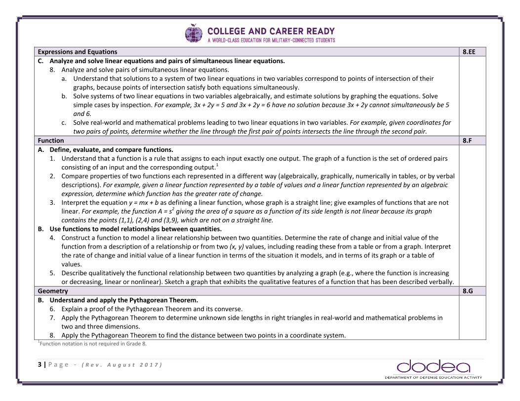
Expressions and Equations 8.EE
C. Analyze and solve linear equations and pairs of simultaneous linear equations. 8. Analyze and solve pairs of simultaneous linear equations.
a. Understand that solutions to a system of two linear equations in two variables correspond to points of intersection of their graphs, because points of intersection satisfy both equations simultaneously.
b. Solve systems of two linear equations in two variables algebraically, and estimate solutions by graphing the equations. Solve simple cases by inspection. For example, 3x + 2y = 5 and 3x + 2y = 6 have no solution because 3x + 2y cannot simultaneously be 5 and 6.
c. Solve real-world and mathematical problems leading to two linear equations in two variables. For example, given coordinates for two pairs of points, determine whether the line through the first pair of points intersects the line through the second pair.
Function 8.F
A. Define, evaluate, and compare functions. 1. Understand that a function is a rule that assigns to each input exactly one output. The graph of a function is the set of ordered pairs
consisting of an input and the corresponding output.1 2. Compare properties of two functions each represented in a different way (algebraically, graphically, numerically in tables, or by verbal
descriptions). For example, given a linear function represented by a table of values and a linear function represented by an algebraic expression, determine which function has the greater rate of change.
3. Interpret the equation y = mx + b as defining a linear function, whose graph is a straight line; give examples of functions that are not linear. For example, the function A = s2 giving the area of a square as a function of its side length is not linear because its graph contains the points (1,1), (2,4) and (3,9), which are not on a straight line.
B. Use functions to model relationships between quantities. 4. Construct a function to model a linear relationship between two quantities. Determine the rate of change and initial value of the
function from a description of a relationship or from two (x, y) values, including reading these from a table or from a graph. Interpret the rate of change and initial value of a linear function in terms of the situation it models, and in terms of its graph or a table of values.
5. Describe qualitatively the functional relationship between two quantities by analyzing a graph (e.g., where the function is increasing or decreasing, linear or nonlinear). Sketch a graph that exhibits the qualitative features of a function that has been described verbally.
Geometry 8.G
B. Understand and apply the Pythagorean Theorem. 6. Explain a proof of the Pythagorean Theorem and its converse. 7. Apply the Pythagorean Theorem to determine unknown side lengths in right triangles in real-world and mathematical problems in
two and three dimensions. 8. Apply the Pythagorean Theorem to find the distance between two points in a coordinate system.
1Function notation is not required in Grade 8.

4 | P a g e - ( R e v . A u g u s t 2 0 1 7 )
Statistics and Probability 8.SP
A. Investigate patterns of association in bivariate data. 1. Construct and interpret scatter plots for bivariate measurement data to investigate patterns of association between two quantities.
Describe patterns such as clustering, outliers, positive or negative association, linear association, and nonlinear association. 2. Know that straight lines are widely used to model relationships between two quantitative variables. For scatter plots that suggest a
linear association, informally fit a straight line, and informally assess the model fit by judging the closeness of the data points to the line.
3. Use the equation of a linear model to solve problems in the context of bivariate measurement data, interpreting the slope and intercept. For example, in a linear model for a biology experiment, interpret a slope of 1.5 cm/hr as meaning that an additional hour of sunlight each day is associated with an additional 1.5 cm in mature plant height.
4. Understand that patterns of association can also be seen in bivariate categorical data by displaying frequencies and relative frequencies in a two-way table. Construct and interpret a two-way table summarizing data on two categorical variables collected from the same subjects. Use relative frequencies calculated for rows or columns to describe possible association between the two variables. For example, collect data from students in your class on whether or not they have a curfew on school nights and whether or not they have assigned chores at home. Is there evidence that those who have a curfew also tend to have chores?
5 | P a g e - ( R e v . A u g u s t 2 0 1 7 )
Standards for Mathematics: Math 8/Algebra 1
The Algebra 1 content of this accelerated course domains, clusters, and standards from five of the six high school conceptual categories (Number and Quantity, Algebra, Functions, Modeling, and Statistics and Probability). The modeling standards aren’t separated into their own category, but dispersed throughout the others and indicated with a *. Students will build their learning of the 8th grade content standards simultaneously with the identified standards for high school Algebra 1.
As such, students in Math 8/Algebra 1 will study in depth linear and exponential relationships and contrasting them, using linear models for data that appear to have a linear trend, and understanding when exponential models are appropriate in various contexts. Students will also engage in methods for solving quadratic functions, analyzing and determine the proper use for quadratics with given quantities. Through the content, students will build mathematical habits of mind as described by the Standards for Mathematical Practice (SMPs).
6 | P a g e - ( R e v . A u g u s t 2 0 1 7 )
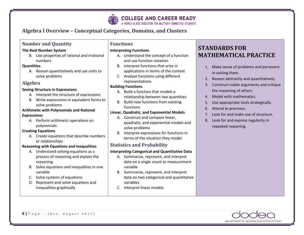
Algebra I Overview – Conceptual Categories, Domains, and Clusters
Number and Quantity
The Real Number System B. Use properties of rational and irrational
numbers Quantities
A. Reason quantitatively and use units to solve problems
Algebra Seeing Structure in Expressions
A. Interpret the structure of expressions B. Write expressions in equivalent forms to
solve problems Arithmetic with Polynomials and Rational Expressions
A. Perform arithmetic operations on polynomials
Creating Equations A. Create equations that describe numbers
or relationships Reasoning with Equations and Inequalities
A. Understand solving equations as a process of reasoning and explain the reasoning
B. Solve equations and inequalities in one variable
C. Solve systems of equations D. Represent and solve equations and
inequalities graphically
Functions
Interpreting Functions A. Understand the concept of a function
and use function notation B. Interpret functions that arise in
applications in terms of the context C. Analyze functions using different
representations Building Functions
A. Build a function that models a relationship between two quantities
B. Build new functions from existing functions
Linear, Quadratic, and Exponential Models A. Construct and compare linear,
quadratic, and exponential models and solve problems
B. Interpret expressions for functions in terms of the situation they model
Statistics and Probability Interpreting Categorical and Quantitative Data
A. Summarize, represent, and interpret data on a single count or measurement variable
B. Summarize, represent, and interpret data on two categorical and quantitative variables
C. Interpret linear models
STANDARDS FOR MATHEMATICAL PRACTICE
1. Make sense of problems and persevere
in solving them.
2. Reason abstractly and quantitatively.
3. Construct viable arguments and critique
the reasoning of others.
4. Model with mathematics.
5. Use appropriate tools strategically.
6. Attend to precision.
7. Look for and make use of structure.
8. Look for and express regularity in
repeated reasoning.

7 | P a g e - ( R e v . A u g u s t 2 0 1 7 )
Number and Quantity
The Real Number System N—RN
B. Use properties of rational and irrational numbers. 3. Explain why the sum or product of two rational numbers is rational; that the sum of a rational number and an irrational number is
irrational; and that the product of a nonzero rational number and an irrational number is irrational.
Quantities* N—Q
A. Reason quantitatively and use units to solve problems. 1. Use units as a way to understand problems and to guide the solution of multi-step problems; choose and interpret units
consistently in formulas; choose and interpret the scale and the origin in graphs and data displays. 2. Define appropriate quantities for the purpose of descriptive modeling. 3. Choose a level of accuracy appropriate to limitations on measurement when reporting quantities.
Algebra
Seeing Structure in Expressions A—SSE
A. Interpret the structure of expressions 1. Interpret expressions that represent a quantity in terms of its context.*
a. Interpret parts of an expression, such as terms, factors, and coefficients. b. Interpret complicated expressions by viewing one or more of their parts as a single entity. For example, interpret P(1+r)n as the
product of P and a factor not depending on P. 2. Use the structure of an expression to identify ways to rewrite it. For example, see x4 – y4 as (x2)2 – (y2)2, thus recognizing it as a
difference of squares that can be factored as (x2 – y2)(x2 + y2). B. Write expressions in equivalent forms to solve problems
3. Choose and produce an equivalent form of an expression to reveal and explain properties of the quantity represented by the expression.* a. Factor a quadratic expression to reveal the zeros of the function it defines. b. Complete the square in a quadratic expression to reveal the maximum or minimum value of the function it defines. c. Use the properties of exponents to transform expressions for exponential functions. For example the expression 1.15t can be
rewritten as (1.151/12)12t ≈ 1.01212t to reveal the approximate equivalent monthly interest rate if the annual rate is 15%.
Arithmetic with Polynomials and Rational Expressions A—APR
A. Perform arithmetic operations on polynomials 1. Understand that polynomials form a system analogous to the integers, namely, they are closed under the operations of addition,
subtraction, and multiplication; add, subtract, and multiply polynomials.
8 | P a g e - ( R e v . A u g u s t 2 0 1 7 )
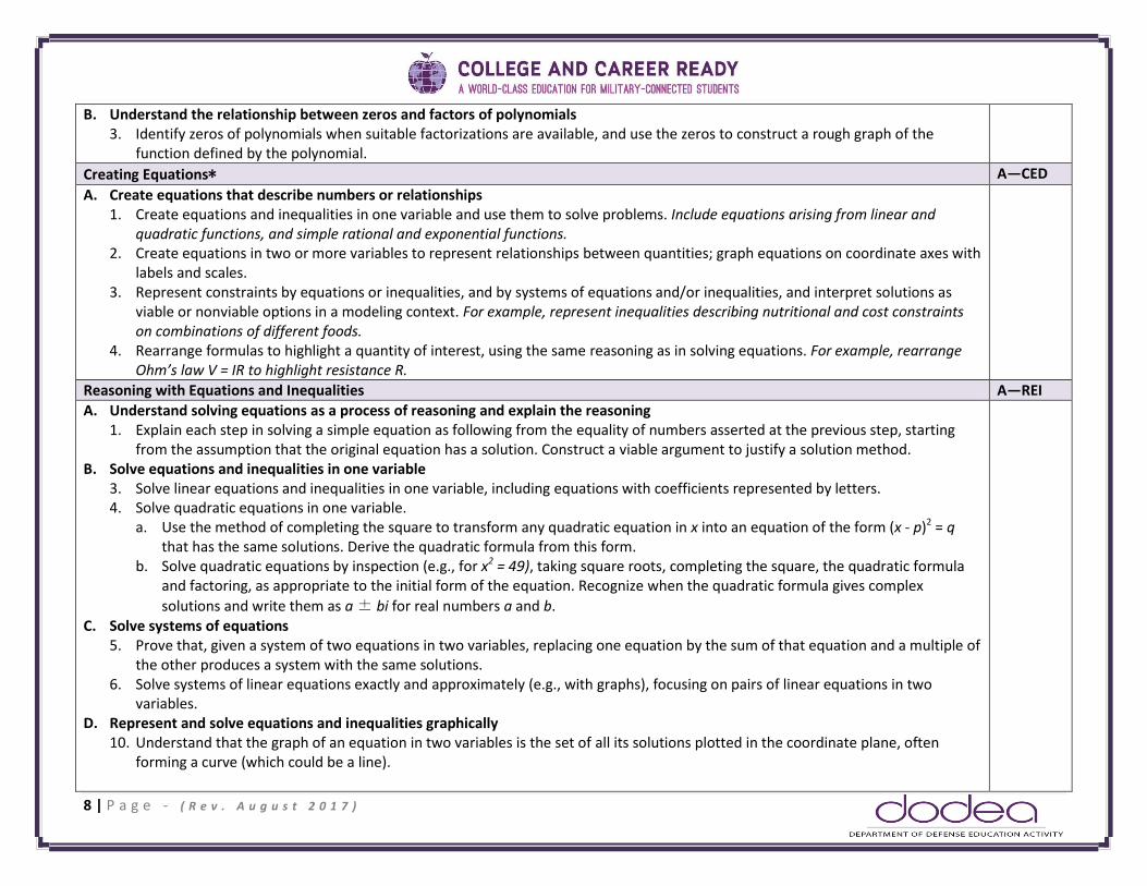
B. Understand the relationship between zeros and factors of polynomials 3. Identify zeros of polynomials when suitable factorizations are available, and use the zeros to construct a rough graph of the
function defined by the polynomial.
Creating Equations* A—CED
A. Create equations that describe numbers or relationships 1. Create equations and inequalities in one variable and use them to solve problems. Include equations arising from linear and
quadratic functions, and simple rational and exponential functions. 2. Create equations in two or more variables to represent relationships between quantities; graph equations on coordinate axes with
labels and scales. 3. Represent constraints by equations or inequalities, and by systems of equations and/or inequalities, and interpret solutions as
viable or nonviable options in a modeling context. For example, represent inequalities describing nutritional and cost constraints on combinations of different foods.
4. Rearrange formulas to highlight a quantity of interest, using the same reasoning as in solving equations. For example, rearrange Ohm’s law V = IR to highlight resistance R.
Reasoning with Equations and Inequalities A—REI
A. Understand solving equations as a process of reasoning and explain the reasoning 1. Explain each step in solving a simple equation as following from the equality of numbers asserted at the previous step, starting
from the assumption that the original equation has a solution. Construct a viable argument to justify a solution method. B. Solve equations and inequalities in one variable
3. Solve linear equations and inequalities in one variable, including equations with coefficients represented by letters. 4. Solve quadratic equations in one variable.
a. Use the method of completing the square to transform any quadratic equation in x into an equation of the form (x - p)2 = q that has the same solutions. Derive the quadratic formula from this form.
b. Solve quadratic equations by inspection (e.g., for x2 = 49), taking square roots, completing the square, the quadratic formula and factoring, as appropriate to the initial form of the equation. Recognize when the quadratic formula gives complex
solutions and write them as a ± bi for real numbers a and b. C. Solve systems of equations
5. Prove that, given a system of two equations in two variables, replacing one equation by the sum of that equation and a multiple of the other produces a system with the same solutions.
6. Solve systems of linear equations exactly and approximately (e.g., with graphs), focusing on pairs of linear equations in two variables.
D. Represent and solve equations and inequalities graphically 10. Understand that the graph of an equation in two variables is the set of all its solutions plotted in the coordinate plane, often
forming a curve (which could be a line).

9 | P a g e - ( R e v . A u g u s t 2 0 1 7 )
11. Explain why the x-coordinates of the points where the graphs of the equations y = f(x) and y = g(x) intersect are the solutions of the equation f(x) = g(x); find the solutions approximately, e.g., using technology to graph the functions, make tables of values, or find successive approximations. Include cases where f(x) and/or g(x) are linear, polynomial, rational, absolute value, exponential,
and logarithmic functions.* 12. Graph the solutions to a linear inequality in two variables as a half plane (excluding the boundary in the case of a strict inequality),
and graph the solution set to a system of linear inequalities in two variables as the intersection of the corresponding half-planes.
Functions
Interpreting Functions F—IF
A. Understand the concept of a function and use function notation 1. Understand that a function from one set (called the domain) to another set (called the range) assigns to each element of the
domain exactly one element of the range. If f is a function and x is an element of its domain, then f(x) denotes the output of f corresponding to the input x. The graph of f is the graph of the equation y = f(x).
2. Use function notation, evaluate functions for inputs in their domains, and interpret statements that use function notation in terms of a context.
3. Recognize that sequences are functions, sometimes defined recursively, whose domain is a subset of the integers. For example, the Fibonacci sequence is defined recursively by f(0) = f(1) = 1, f(n+1) = f(n) + f(n-1) for n ≥ 1.
B. Interpret functions that arise in applications in terms of the context 4. For a function that models a relationship between two quantities, interpret key features of graphs and tables in terms of the
quantities, and sketch graphs showing key features given a verbal description of the relationship. Key features include: intercepts; intervals where the function is increasing, decreasing, positive, or negative; relative maximums and minimums; symmetries; end behavior; and periodicity.*
5. Relate the domain of a function to its graph and, where applicable, to the quantitative relationship it describes. For example, if the function h(n) gives the number of person-hours it takes to assemble n engines in a factory, then the positive integers would be an appropriate domain for the function. *
6. Calculate and interpret the average rate of change of a function (presented symbolically or as a table) over a specified interval. Estimate the rate of change from a graph. *
C. Analyze functions using different representations 7. Graph functions expressed symbolically and show key features of the graph, by hand in simple cases and using technology for
more complicated cases. * a. Graph linear and quadratic functions and show intercepts, maxima, and minima. b. Graph square root, cube root, and piecewise-defined functions, including step functions and absolute value functions.

10 | P a g e - ( R e v . A u g u s t 2 0 1 7 )
8. Write a function defined by an expression in different but equivalent forms to reveal and explain different properties of the function. a. Use the process of factoring and completing the square in a quadratic function to show zeros, extreme values, and symmetry
of the graph, and interpret these in terms of a context. 9. Compare properties of two functions each represented in a different way (algebraically, graphically, numerically in tables, or by
verbal descriptions). For example, given a graph of one quadratic function and an algebraic expression for another, say which has the larger maximum.
Building Functions F—BF
A. Build a function that models a relationship between two quantities
1. Write a function that describes a relationship between two quantities.* a. Determine an explicit expression, a recursive process, or steps for calculation from a context.
B. Build new functions from existing functions 3. Identify the effect on the graph of replacing f(x) by f(x) + k, k f(x), f(kx), and f(x + k) for specific values of k (both positive and
negative); find the value of k given the graphs. Experiment with cases and illustrate an explanation of the effects on the graph using technology. Include recognizing even and odd functions from their graphs and algebraic expressions for them.
Linear, Quadratic, and Exponential Models* F—LE
A. Construct and compare linear, quadratic, and exponential models and solve problems 1. Distinguish between situations that can be modeled with linear functions and with exponential functions.
a. Prove that linear functions grow by equal differences over equal intervals, and that exponential functions grow by equal factors over equal intervals.
b. Recognize situations in which one quantity changes at a constant rate per unit interval relative to another. c. Recognize situations in which a quantity grows or decays by a constant percent rate per unit interval relative to another.
2. Construct linear and exponential functions, including arithmetic and geometric sequences, given a graph, a description of a relationship, or two input-output pairs (include reading these from a table).
3. Observe using graphs and tables that a quantity increasing exponentially eventually exceeds a quantity increasing linearly, quadratically, or (more generally) as a polynomial function.
B. Interpret expressions for functions in terms of the situation they model 5. Interpret the parameters in a linear or exponential function in terms of a context.
Statistics and Probability
Interpreting Categorical and Quantitative Data S—ID
A. Summarize, represent, and interpret data on a single count or measurement variable 1. Represent data with plots on the real number line (dot plots, histograms, and box plots). 2. Use statistics appropriate to the shape of the data distribution to compare center (median, mean) and spread (interquartile range,
standard deviation) of two or more different data sets.

11 | P a g e - ( R e v . A u g u s t 2 0 1 7 )
3. Interpret differences in shape, center, and spread in the context of the data sets, accounting for possible effects of extreme data points (outliers).
4. Use the mean and standard deviation of a data set to fit it to a normal distribution and to estimate population percentages. Recognize that there are data sets for which such a procedure is not appropriate. Use calculators, spreadsheets, and tables to estimate areas under the normal curve.
B. Summarize, represent, and interpret data on two categorical and quantitative variables 5. Summarize categorical data for two categories in two-way frequency tables. Interpret relative frequencies in the context of the
data (including joint, marginal, and conditional relative frequencies). Recognize possible associations and trends in the data. 6. Represent data on two quantitative variables on a scatter plot, and describe how the variables are related.
a. Fit a function to the data; use functions fitted to data to solve problems in the context of the data. Use given functions or choose a function suggested by the context. Emphasize linear, quadratic, and exponential models.
b. Informally assess the fit of a function by plotting and analyzing residuals. c. Fit a linear function for a scatter plot that suggests a linear association.
C. Interpret linear models 7. Interpret the slope (rate of change) and the intercept (constant term) of a linear model in the context of the data. 8. Compute (using technology) and interpret the correlation coefficient of a linear fit. 9. Distinguish between correlation and causation.

12 | P a g e - ( R e v . A u g u s t 2 0 1 7 )
Glossary Addition and subtraction within 5, 10, 20, 100, or 1000. Addition or subtraction of two whole numbers with whole number answers, and with sum or minuend in the range 0-5, 0-10, 0-20, or 0-100, respectively. Example: 8 + 2 = 10 is an addition within 10, 14 – 5 = 9 is a subtraction within 20, and 55 – 18 = 37 is a subtraction within 100.
Additive inverses. Two numbers whose sum is 0 are additive inverses of one another. Example: 3/4 and – 3/4 are additive inverses of one another because 3/4 + (– 3/4) = (– 3/4) + 3/4 = 0.
Associative property of addition. See Table 3 in this Glossary.
Associative property of multiplication. See Table 3 in this Glossary.
Bivariate data. Pairs of linked numerical observations. Example: a list of heights and weights for each player on a football team.
Box plot. A method of visually displaying a distribution of data values by using the median, quartiles, and extremes of the data set. A box shows the middle 50% of the data.1
Commutative property. See Table 3 in this Glossary.
Complex fraction. A fraction A/B where A and/or B are fractions (B nonzero).
Computation algorithm. A set of predefined steps applicable to a class of problems that gives the correct result in every case when the steps are carried out correctly. See also: computation strategy.
Computation strategy. Purposeful manipulations that may be chosen for specific problems, may not have a fixed order, and may be aimed at converting one problem into another. See also: computation algorithm.
Congruent. Two plane or solid figures are congruent if one can be obtained from the other by rigid motion (a sequence of rotations, reflections, and translations).
Counting on. A strategy for finding the number of objects in a group without having to count every member of the group. For example, if a stack of books is known to have 8 books and 3 more books are added to the top, it is not necessary to count the stack all over again. One can find the total by counting on—pointing to the top book and saying “eight,” following this with “nine, ten, eleven. There are eleven books now.”
Dot plot. See: line plot.
1Adapted from Wisconsin Department of Public Instruction, http://dpi.wi.gov/standards/mathglos.html, accessed March 2, 2010.

13 | P a g e - ( R e v . A u g u s t 2 0 1 7 )
Dilation. A transformation that moves each point along the ray through the point emanating from a fixed center, and multiplies distances from the center by a common scale factor.
Expanded form. A multi-digit number is expressed in expanded form when it is written as a sum of single-digit multiples of powers of ten. For example, 643 = 600 + 40 + 3.
Expected value. For a random variable, the weighted average of its possible values, with weights given by their respective probabilities.
First quartile. For a data set with median M, the first quartile is the median of the data values less than M. Example: For the data set {1, 3, 6, 7, 10, 12, 14, 15, 22, 120}, the first quartile is 6.2 See also: median, third quartile, interquartile range.
Fraction. A number expressible in the form a/b where a is a whole number and b is a positive whole number. (The word fraction in these standards always refers to a non-negative number.) See also: rational number.
Identity property of 0. See Table 3 in this Glossary.
Independently combined probability models. Two probability models are said to be combined independently if the probability of each ordered pair in the combined model equals the product of the original probabilities of the two individual outcomes in the ordered pair.
Integer. A number expressible in the form a or –a for some whole number a.
Interquartile Range. A measure of variation in a set of numerical data, the interquartile range is the distance between the first and third quartiles of the data set. Example: For the data set {1, 3, 6, 7, 10, 12, 14, 15, 22, 120}, the interquartile range is 15 – 6 = 9. See also: first quartile, third quartile.
Line plot. A method of visually displaying a distribution of data values where each data value is shown as a dot or mark above a number line. Also known as a dot plot.3
Mean. A measure of center in a set of numerical data, computed by adding the values in a list and then dividing by the number of values in the list.4 Example: For the data set {1, 3, 6, 7, 10, 12, 14, 15, 22, 120}, the mean is 21.
Mean absolute deviation. A measure of variation in a set of numerical data, computed by adding the distances between each data value and the mean, then dividing by the number of data values. Example: For the data set {2, 3, 6, 7, 10, 12, 14, 15, 22, 120}, the mean absolute deviation is 20.
2Many different methods for computing quartiles are in use. The method defined here is sometimes called the Moore and McCabe method. See Langford, E., “Quartiles in Elementary
Statistics,” Journal of Statistics Education Volume 14, Number 3 (2006). 3Adapted from Wisconsin Department of Public Instruction, op. cit.
4To be more precise, this defines the arithmetic mean.

14 | P a g e - ( R e v . A u g u s t 2 0 1 7 )
Median. A measure of center in a set of numerical data. The median of a list of values is the value appearing at the center of a sorted version of the list—or the mean of the two central values, if the list contains an even number of values. Example: For the data set {2, 3, 6, 7, 10, 12, 14, 15, 22, 90}, the median is 11.
Midline. In the graph of a trigonometric function, the horizontal line halfway between its maximum and minimum values.
Multiplication and division within 100. Multiplication or division of two whole numbers with whole number answers, and with product or dividend in the range 0-100. Example: 72 ÷ 8 = 9.
Multiplicative inverses. Two numbers whose product is 1 are multiplicative inverses of one another. Example: 3/4 and 4/3 are multiplicative inverses of one another because 3/4 × 4/3 = 4/3 × 3/4 = 1.
Number line diagram. A diagram of the number line used to represent numbers and support reasoning about them. In a number line diagram for measurement quantities, the interval from 0 to 1 on the diagram represents the unit of measure for the quantity.
Percent rate of change. A rate of change expressed as a percent. Example: if a population grows from 50 to 55 in a year, it grows by 5/50 = 10% per year.
Probability distribution. The set of possible values of a random variable with a probability assigned to each.
Properties of operations. See Table 3 in this Glossary.
Properties of equality. See Table 4 in this Glossary.
Properties of inequality. See Table 5 in this Glossary.
Properties of operations. See Table 3 in this Glossary.
Probability. A number between 0 and 1 used to quantify likelihood for processes that have uncertain outcomes (such as tossing a coin, selecting a person at random from a group of people, tossing a ball at a target, or testing for a medical condition).
Probability model. A probability model is used to assign probabilities to outcomes of a chance process by examining the nature of the process. The set of all outcomes is called the sample space, and their probabilities sum to 1. See also: uniform probability model.
Random variable. An assignment of a numerical value to each outcome in a sample space.
Rational expression. A quotient of two polynomials with a non-zero denominator.
Rational number. A number expressible in the form a/b or – a/b for some fraction a/b. The rational numbers include the integers.
15 | P a g e - ( R e v . A u g u s t 2 0 1 7 )
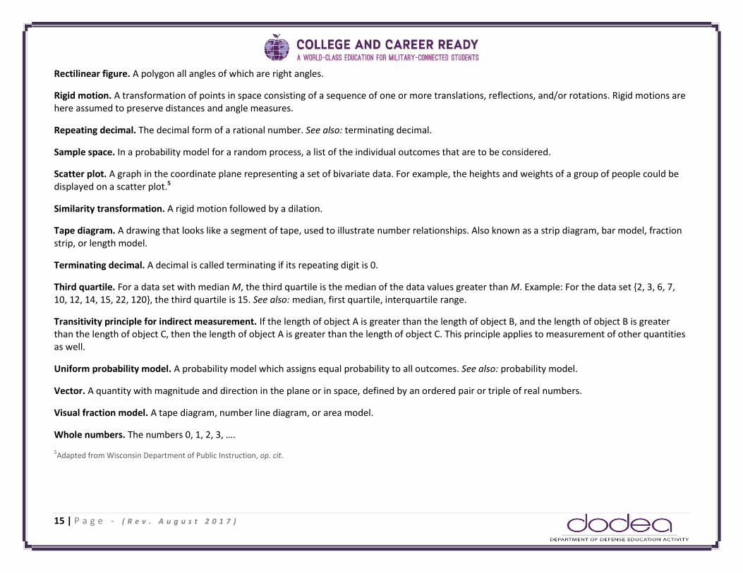
Rectilinear figure. A polygon all angles of which are right angles.
Rigid motion. A transformation of points in space consisting of a sequence of one or more translations, reflections, and/or rotations. Rigid motions are here assumed to preserve distances and angle measures.
Repeating decimal. The decimal form of a rational number. See also: terminating decimal.
Sample space. In a probability model for a random process, a list of the individual outcomes that are to be considered.
Scatter plot. A graph in the coordinate plane representing a set of bivariate data. For example, the heights and weights of a group of people could be displayed on a scatter plot.5
Similarity transformation. A rigid motion followed by a dilation.
Tape diagram. A drawing that looks like a segment of tape, used to illustrate number relationships. Also known as a strip diagram, bar model, fraction strip, or length model.
Terminating decimal. A decimal is called terminating if its repeating digit is 0.
Third quartile. For a data set with median M, the third quartile is the median of the data values greater than M. Example: For the data set {2, 3, 6, 7, 10, 12, 14, 15, 22, 120}, the third quartile is 15. See also: median, first quartile, interquartile range.
Transitivity principle for indirect measurement. If the length of object A is greater than the length of object B, and the length of object B is greater than the length of object C, then the length of object A is greater than the length of object C. This principle applies to measurement of other quantities as well.
Uniform probability model. A probability model which assigns equal probability to all outcomes. See also: probability model.
Vector. A quantity with magnitude and direction in the plane or in space, defined by an ordered pair or triple of real numbers.
Visual fraction model. A tape diagram, number line diagram, or area model.
Whole numbers. The numbers 0, 1, 2, 3, ….
5Adapted from Wisconsin Department of Public Instruction, op. cit.
16 | P a g e - ( R e v . A u g u s t 2 0 1 7 )
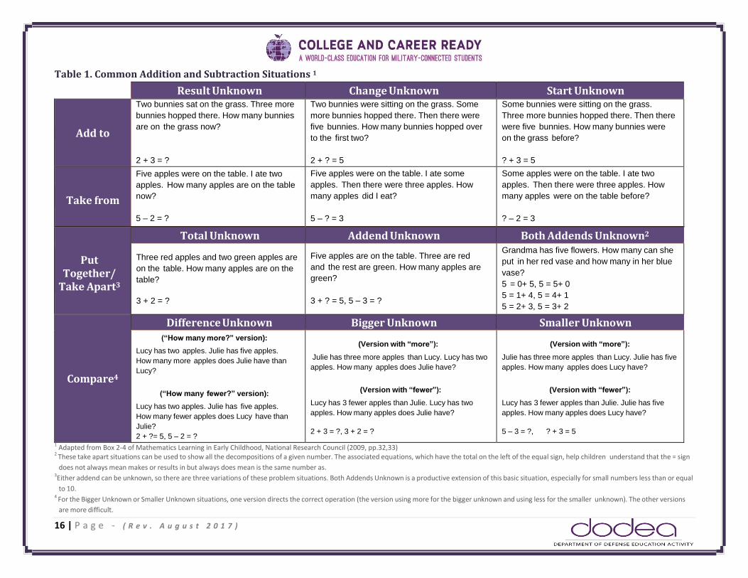
Table 1. Common Addition and Subtraction Situations 1
Result Unknown Change Unknown Start Unknown
Add to
Two bunnies sat on the grass. Three more
bunnies hopped there. How many bunnies
are on the grass now?
2 + 3 = ?
Two bunnies were sitting on the grass. Some
more bunnies hopped there. Then there were
five bunnies. How many bunnies hopped over
to the first two?
2 + ? = 5
Some bunnies were sitting on the grass.
Three more bunnies hopped there. Then there
were five bunnies. How many bunnies were
on the grass before?
? + 3 = 5
Take from
Five apples were on the table. I ate two
apples. How many apples are on the table
now?
5 – 2 = ?
Five apples were on the table. I ate some
apples. Then there were three apples. How
many apples did I eat?
5 – ? = 3
Some apples were on the table. I ate two
apples. Then there were three apples. How
many apples were on the table before?
? – 2 = 3
Put Together/
Take Apart3
Total Unknown Addend Unknown Both Addends Unknown2
Three red apples and two green apples are
on the table. How many apples are on the
table?
3 + 2 = ?
Five apples are on the table. Three are red
and the rest are green. How many apples are
green?
3 + ? = 5, 5 – 3 = ?
Grandma has five flowers. How many can she
put in her red vase and how many in her blue
vase?
5 = 0+ 5, 5 = 5+ 0
5 = 1+ 4, 5 = 4+ 1
5 = 2+ 3, 5 = 3+ 2
Compare4
Difference Unknown Bigger Unknown Smaller Unknown (“How many more?” version):
Lucy has two apples. Julie has five apples.
How many more apples does Julie have than
Lucy?
(“How many fewer?” version):
Lucy has two apples. Julie has five apples.
How many fewer apples does Lucy have than
Julie?
2 + ?= 5, 5 – 2 = ?
(Version with “more”):
Julie has three more apples than Lucy. Lucy has two
apples. How many apples does Julie have?
(Version with “fewer”):
Lucy has 3 fewer apples than Julie. Lucy has two
apples. How many apples does Julie have?
2 + 3 = ?, 3 + 2 = ?
(Version with “more”):
Julie has three more apples than Lucy. Julie has five
apples. How many apples does Lucy have?
(Version with “fewer”):
Lucy has 3 fewer apples than Julie. Julie has five
apples. How many apples does Lucy have?
5 – 3 = ?, ? + 3 = 5
1 Adapted from Box 2-4 of Mathematics Learning in Early Childhood, National Research Council (2009, pp.32,33) 2 These take apart situations can be used to show all the decompositions of a given number. The associated equations, which have the total on the left of the equal sign, help children understand that the = sign
does not always mean makes or results in but always does mean is the same number as. 3Either addend can be unknown, so there are three variations of these problem situations. Both Addends Unknown is a productive extension of this basic situation, especially for small numbers less than or equal
to 10. 4 For the Bigger Unknown or Smaller Unknown situations, one version directs the correct operation (the version using more for the bigger unknown and using less for the smaller unknown). The other versions
are more difficult.

17 | P a g e - ( R e v . A u g u s t 2 0 1 7 )
Table 2. Common Multiplication and Division Situations5
Unknown Product Group Size Unknown (“How
many in each group?” Division) Number of Groups Unknown
(“How many groups?” Division)
3 × 6 = ? 3 × ? = 18 and, 18 ÷ 3 = ? ? × 6 = 18, and 18 ÷ 6 = ?
Equal Groups
There are 3 bags with 6 plums in each
bag. How many plums are there in all?
Measurement example. You need 3
lengths of string, each 6 inches long. How
much string will you need altogether?
If 18 plums are shared equally into 3 bags,
then how many plums will be in each bag?
Measurement example. You have 18 inches of
string, which you will cut into 3 equal pieces.
How long will each piece of string be?
If 18 plums are to be packed 6 to a bag, then
how many bags are needed?
Measurement example. You have 18 inches
of string, which you will cut into pieces that are
6 inches long. How many pieces of string will
you have?
Arrays,6
area7
There are 3 rows of apples with 6 apples
in each row. How many apples are there?
Area example. What is the area of a 3 cm
by 6 cm rectangle?
If 18 apples are arranged into 3 equal rows,
how many apples will be in each row?
Area example. A rectangle has area 18
square centimeters. If one side is 3 cm long,
how long is a side next to it?
If 18 apples are arranged into equal rows of 6
apples, how many rows will there be?
Area example. A rectangle has area 18
square centimeters. If one side is 6 cm long,
how long is a side next to it?
Compare
A blue hat costs $6. A red hat costs 3 times
as much as the blue hat. How much does
the red hat cost?
Measurement example. A rubber band is 6
cm long. How long will the rubber band be
when it is stretched to be 3 times as long?
A red hat costs $18 and that is 3 times as
much as a blue hat costs. How much does a
blue hat cost?
Measurement example. A rubber band is
stretched to be 18 cm long and that is 3 times
as long as it was at first. How long was the
rubber band at first?
A red hat costs $18 and a blue hat costs $6.
How many times as much does the red hat
cost as the blue hat?
Measurement example. A rubber band was 6
cm long at first. Now it is stretched to be 18
cm long. How many times as long is the
rubber band now as it was at first?
General a × b = ? a × ? = p, and p ÷ a = ? ? × b = p, and p ÷ b = ?
5 The first examples in each cell are examples of discrete things. These are easier for students and should be given before the measurement examples.
6 The language in the array examples shows the easiest form of array problems. A harder form is to use the terms rows and columns: The apples in the grocery window are in 3 rows and 6
columns. How many apples are in there? Both forms are valuable. 7
Area involves arrays of squares that have been pushed together so that there are no gaps or overlaps, so array problems include these especially important measurement situations.

18 | P a g e - ( R e v . A u g u s t 2 0 1 7 )
Table 3. The Properties of Operations
Here a, b and c stand for arbitrary numbers in a given number system. The properties of operations apply to the rational number system, the real
number system, and the complex number system.
Associative property of addition (a + b) + c = a + (b + c)
Commutative property of addition a + b = b + a
Additive identity property of 0 a + 0 = 0 + a = a
Existence of additive inverses For every a there exists –a so that a + (–a) = (–a) + a = 0.
Associative property of multiplication (a × b) × c = a × (b × c)
Commutative property of multiplication a × b = b × a
Multiplicative identity property of 1 a × 1 = 1 × a = a
Existence of multiplicative inverses For every a ≠ 0 there exists 1/a so that a × 1/a = 1/a × a = 1.
Distributive property of multiplication over addition a × (b + c) = a × b + a × c

19 | P a g e - ( R e v . A u g u s t 2 0 1 7 )
Table 4. The Properties of Equality
Here a, b and c stand for arbitrary numbers in the rational, real, or complex number systems.
Reflexive property of equality a = a
Symmetric property of equality If a = b, then b = a.
Transitive property of equality If a = b and b = c, then a = c.
Addition property of equality If a = b, then a + c = b + c.
Subtraction property of equality If a = b, then a – c = b – c.
Multiplication property of equality If a = b, then a × c = b × c.
Division property of equality If a = b and c ≠ 0, then a ÷ c = b ÷ c.
Substitution property of equality If a = b, then b may be substituted for a in any expression containing a.

20 | P a g e - ( R e v . A u g u s t 2 0 1 7 )
Table 5. The Properties of Inequality
Here a, b and c stand for arbitrary numbers in the rational or real number systems.
Exactly one of the following is true: a < b, a = b, a > b.
If a > b and b > c then a > c.
If a > b, then b < a.
If a > b, then –a < –b.
If a > b, then a ± c > b ± c.
If a > b and c > 0, then a × c > b × c.
If a > b and c < 0, then a × c < b × c.
If a > b and c > 0, then a ÷ c > b ÷ c.
If a > b and c < 0, then a ÷ c < b ÷ c.

21 | P a g e - ( R e v . A u g u s t 2 0 1 7 )

22 | P a g e - ( R e v . A u g u s t 2 0 1 7 )
Sample of Works Consulted Existing state standards documents. Research summaries and briefs provided to the Working Group by researchers. National Assessment Governing Board, Mathematics Framework for the 2009 National Assessment of Educational Progress. U.S. Department of Education, 2008. NAEP Validity Studies Panel, Validity Study of the NAEP Mathematics Assessment: Grades 4 and 8. Daro et al., 2007. Mathematics documents from: Alberta, Canada; Belgium; China; Chinese Taipei; Denmark; England; Finland; Hong Kong; India; Ireland; Japan; Korea; New Zealand; Singapore; Victoria (British Columbia). Adding it Up: Helping Children Learn Mathematics. National Research Council, Mathematics Learning Study Committee, 2001. Benchmarking for Success: Ensuring U.S. Students Receive a World- Class Education. National Governors Association, Council of Chief State School Officers, and Achieve, Inc., 2008. Crossroads in Mathematics (1995) and Beyond Crossroads (2006). American Mathematical Association of Two-Year Colleges (AMATYC).
Curriculum Focal Points for Prekindergarten through Grade 8 Mathematics: A Quest for Coherence. NCTM, 2006. Focus in High School Mathematics: Reasoning and Sense Making. NCTM. Reston, VA: NCTM. Foundations for Success: The Final Report of the National Mathematics Advisory Panel. U.S. Department of Education: Washington, DC, 2008. Guidelines for Assessment and Instruction in Statistics Education (GAISE) Report: A PreK-12 Curriculum Framework. How People Learn: Brain, Mind, Experience, and School. Bransford, J.D., Brown, A.L., and Cocking, R.R., eds. Committee on Developments in the Science of Learning, Commission on Behavioral and Social Sciences and Education, National Research Council, 1999. Mathematics and Democracy, The Case for Quantitative Literacy, Steen, L.A. (ed.). National Council on Education and the Disciplines,
2001.
Mathematics Learning in Early Childhood: Paths Toward Excellence and Equity. Cross, C.T., Woods, T.A., and
Schweingruber, S., eds. Committee on Early Childhood Mathematics, National Research Council, 2009.
The Opportunity Equation: Transforming Mathematics and Science Education for Citizenship and the Global Economy. The Carnegie Corporation of New York and the Institute for Advanced Study, 2009. Online: http://www. opportunityequation.org/ Principles and Standards for School Mathematics. National Council of Teachers of
Mathematics, 2000. The Proficiency Illusion. Cronin, J., Dahlin, M., Adkins, D., and Kingsbury, G.G.; foreword by C.E. Finn, Jr., and M. J. Petrilli. Thomas B. Fordham Institute, 2007. Ready or Not: Creating a High School Diploma That Counts. American Diploma Project, 2004. A Research Companion to Principles and Standards for School Mathematics. NCTM, 2003. Sizing Up State Standards 2008. American Federation of Teachers, 2008. A Splintered Vision: An Investigation of U.S. Science and Mathematics Education. Schmidt, W.H., McKnight, C.C., Raizen, S.A., et al. U.S. National Research Center for the Third International Mathematics and Science Study, Michigan State University, 1997. Stars By Which to Navigate? Scanning National and International Education Standards in 2009. Carmichael, S.B., Wilson. W.S, Finn, Jr., C.E., Winkler, A.M., and Palmieri, S. Thomas B. Fordham Institute, 2009.

23 | P a g e - ( R e v . A u g u s t 2 0 1 7 )
Askey, R., “Knowing and Teaching Elementary Mathematics,” American Educator, Fall 1999.
Aydogan, C., Plummer, C., Kang, S. J., Bilbrey, C., Farran, D. C., and Lipsey, M. W. (2005). An investigation of prekindergarten curricula: Influences on classroom characteristics and child engagement. Paper presented at the NAEYC. Blum, W., Galbraith, P. L., Henn, H-W. and Niss, M. (Eds) Applications and Modeling in Mathematics Education,
ICMI Study 14. Amsterdam: Springer. Brosterman, N. (1997). Inventing kindergarten. New York: Harry N.
Abrams. Clements, D. H., and Sarama, J. (2009). Learning and teaching early math: The learning trajectories approach. New York: Routledge. Clements, D. H., Sarama, J., and DiBiase, A.- M. (2004). Clements, D. H., Sarama, J., and DiBiase, A.-M. (2004). Engaging young children in mathematics: Standards for early childhood mathematics education.
Mahwah, NJ: Lawrence Erlbaum Associates. Cobb and Moore, “Mathematics, Statistics, and Teaching,” Amer. Math. Monthly
104(9), pp. 801-823, 1997. Confrey, J., “Tracing the Evolution of Mathematics Content Standards in the United States: Looking Back and Projecting Forward.” K12 Mathematics Curriculum Standards conference proceedings, February 5-6, 2007.
Conley, D.T. Knowledge and Skills for University Success, 2008. Conley, D.T. Toward a More Comprehensive Conception of College Readiness, 2007. Cuoco, A., Goldenberg, E. P., and Mark, J., “Habits of Mind: An Organizing Principle for a Mathematics Curriculum,” Journal of Mathematical Behavior, 15(4), 375-402, 1996. Carpenter, T. P., Fennema, E., Franke, M. L., Levi, L., and Empson, S. B. (1999). Children’s Mathematics: Cognitively Guided Instruction. Portsmouth, NH: Heinemann. Van de Walle, J. A., Karp, K., and Bay- Williams, J. M. (2010). Elementary and Middle School Mathematics: Teaching Developmentally (Seventh ed.). Boston: Allyn and Bacon. Ginsburg, A., Leinwand, S., and Decker, K., “Informing Grades 1-6 Standards Development: What Can Be Learned from High-Performing Hong Kong, Korea, and Singapore?” American Institutes for Research, 2009. Ginsburg et al., “What the United States Can Learn From Singapore’s World- Class Mathematics System (and what Singapore can learn from the United States),” American Institutes for Research, 2005. Ginsburg et al., “Reassessing U.S. International Mathematics Performance: New Findings from the 2003 TIMMS and PISA,” American Institutes for Research, 2005.
Ginsburg, H. P., Lee, J. S., and Stevenson- Boyd, J. (2008). Mathematics education for young children: What it is and how to promote it. Social Policy Report, 22(1), 1-24. Harel, G., “What is Mathematics? A Pedagogical Answer to a Philosophical Question,” in R. B. Gold and R. Simons (eds.), Current Issues in the Philosophy of Mathematics from the Perspective of Mathematicians. Mathematical Association of America, 2008. Henry, V. J., and Brown, R. S. (2008). First grade basic facts: An investigation into teaching and learning of an accelerated, high-demand memorization standard. Journal for Research in Mathematics Education, 39, 153-183. Howe, R., “From Arithmetic to Algebra.” Howe, R., “Starting Off Right in Arithmetic,” http://math.arizona. edu/~ime/2008-09/MIME/BegArith.pdf. Jordan, N. C., Kaplan, D., Ramineni, C., and Locuniak, M. N., “Early math matters: kindergarten number competence and later mathematics outcomes,” Dev. Psychol. 45, 850–867, 2009. Kader, G., “Means and MADS,” Mathematics Teaching in the Middle School, 4(6), 1999, pp. 398-403.
Kilpatrick, J., Mesa, V., and Sloane, F., “U.S. Algebra Performance in an International Context,” in Loveless (ed.), Lessons Learned: What International Assessments Tell Us About Math Achievement. Washington, D.C.: Brookings Institution Press, 2007.

24 | P a g e - ( R e v . A u g u s t 2 0 1 7 )
Leinwand, S., and Ginsburg, A., “Measuring Up: How the Highest Performing State (Massachusetts) Compares to the Highest Performing Country (Hong Kong) in Grade 3 Mathematics,” American Institutes for Research, 2009. Niss, M., “Quantitative Literacy and Mathematical Competencies,” in Quantitative Literacy: Why Numeracy Matters for Schools and Colleges, Madison, B. L., and Steen, L.A. (eds.), National Council on Education and the Disciplines. Proceedings of the National Forum on Quantitative Literacy held at the National Academy of Sciences in Washington, D.C., December 1-2, 2001. Pratt, C. (1948). I learn from children. New York: Simon and Schuster. Reys, B. (ed.), The Intended Mathematics Curriculum as Represented in State- Level Curriculum Standards: Consensus or Confusion? IAP-Information Age Publishing, 2006. Sarama, J., and Clements, D. H. (2009). Early childhood mathematics education research: Learning trajectories for young children. New York: Routledge. Schmidt, W., Houang, R., and Cogan, L., “A Coherent Curriculum: The Case of Mathematics,” American Educator,
Summer 2002, p. 4.
Schmidt, W.H., and Houang, R.T., “Lack of Focus in the Intended Mathematics Curriculum: Symptom or Cause?” in Loveless (ed.), Lessons Learned: What International Assessments Tell Us About Math Achievement. Washington, D.C.:
Brookings Institution Press, 2007. Steen, L.A., “Facing Facts: Achieving Balance in High School Mathematics.” Mathematics Teacher, Vol. 100. Special Issue. Wu, H., “Fractions, decimals, and rational numbers,” 2007, http://math.berkeley. edu/~wu/ (March 19, 2008). Wu, H., “Lecture Notes for the 2009 Pre- Algebra Institute,” September 15, 2009. Wu, H., “Preservice professional development of mathematics teachers,” http://math.berkeley.edu/~wu/pspd2. pdf. Massachusetts Department of Education. Progress Report of the Mathematics Curriculum Framework Revision Panel, Massachusetts Department of Elementary and Secondary Education, 2009. www.doe.mass.edu/boe/docs/0509/ item5_report.pdf. ACT College Readiness Benchmarks™ ACT College Readiness Standards™ ACT National Curriculum Survey™
Adelman, C., The Toolbox Revisited: Paths to Degree Completion From High School Through College, 2006. Advanced Placement Calculus, Statistics and Computer Science Course Descriptions. May 2009, May 2010. College Board, 2008. Aligning Postsecondary Expectations and High School Practice: The Gap Defined (ACT: Policy Implications of the ACT National Curriculum Survey Results 2005-2006). Condition of Education, 2004: Indicator 30, Top 30 Postsecondary Courses, U.S. Department of Education, 2004. Condition of Education, 2007: High School Course-Taking. U.S. Department of Education, 2007. Crisis at the Core: Preparing All Students for College and Work, ACT. Achieve, Inc., Florida Postsecondary Survey, 2008. Golfin, Peggy, et al. CNA Corporation. Strengthening Mathematics at the Postsecondary Level: Literature Review and Analysis, 2005. Camara, W.J., Shaw, E., and Patterson, B. (June 13, 2009). First Year English and Math College Coursework. College Board: New York, NY (Available from authors). CLEP Precalculus Curriculum Survey: Summary of Results. The College Board, 2005.

25 | P a g e - ( R e v . A u g u s t 2 0 1 7 )
College Board Standards for College Success: Mathematics and Statistics. College Board, 2006. Miller, G.E., Twing, J., and Meyers, J. “Higher Education Readiness Component (HERC) Correlation Study.” Austin, TX: Pearson. On Course for Success: A Close Look at Selected High School Courses That Prepare All Students for College and Work, ACT. Out of Many, One: Towards Rigorous Common Core Standards from the Ground Up. Achieve, 2008. Ready for College and Ready for Work: Same or Different? ACT. Rigor at Risk: Reaffirming Quality in the High School Core Curriculum, ACT. The Forgotten Middle: Ensuring that All Students Are on Target for College and Career Readiness before High School,
ACT. Achieve, Inc., Virginia Postsecondary Survey, 2004. ACT Job Skill Comparison Charts. Achieve, Mathematics at Work, 2008. The American Diploma Project Workplace Study. National Alliance of Business Study, 2002.
Carnevale, Anthony and Desrochers, Donna. Connecting Education Standards and Employment: Coursetaking Patterns of Young Workers, 2002. Colorado Business Leaders’ Top Skills, 2006. Hawai’i Career Ready Study: access to living wage careers from high school,
2007. States’ Career Cluster Initiative. Essential Knowledge and Skill Statements, 2008.
ACT WorkKeys Occupational Profiles™. Program for International Student Assessment (PISA), 2006. Trends in International Mathematics and Science Study (TIMSS), 2007.
International Baccalaureate, Mathematics Standard Level, 2006. University of Cambridge International Examinations: General Certificate of Secondary Education in Mathematics, 2009. EdExcel, General Certificate of Secondary Education, Mathematics, 2009. Blachowicz, Camille, and Fisher, Peter. “Vocabulary Instruction.” In Handbook of Reading Research, Volume III, edited by Michael Kamil, Peter Mosenthal, P. David Pearson, and Rebecca Barr, pp. 503-523. Mahwah, NJ: Lawrence Erlbaum Associates, 2000.
Gándara, Patricia, and Contreras, Frances. The Latino Education Crisis: The Consequences of Failed Social Policies.
Cambridge, Ma: Harvard University Press, 2009. Moschkovich, Judit N. “Supporting the Participation of English Language Learners in Mathematical Discussions.” For the Learning of Mathematics 19 (March 1999): 11-19. Moschkovich, J. N. (in press). Language, culture, and equity in secondary mathematics classrooms. To appear in F. Lester and J. Lobato (ed.), Teaching and Learning Mathematics: Translating Research to the Secondary Classroom, Reston, VA: NCTM. Moschkovich, Judit N. “Examining Mathematical Discourse Practices,” For the Learning of Mathematics 27 (March
2007): 24-30.
Moschkovich, Judit N. “Using Two Languages when Learning Mathematics: How Can Research Help Us Understand Mathematics Learners Who Use Two Languages?” Research Brief and Clip, National Council of Teachers of
Mathematics, 2009 http://www.nctm. org/uploadedFiles/Research_News_ and_Advocacy/Research/Clips_and_ Briefs/Research_brief_12_Using_2.pdf. (accessed November 25, 2009).

26 | P a g e - ( R e v . A u g u s t 2 0 1 7 )
Moschkovich, J.N. (2007) Bilingual Mathematics Learners: How views of language, bilingual learners, and mathematical communication impact instruction. In Nasir, N. and Cobb, P. (eds.), Diversity, Equity, and Access to Mathematical Ideas. New York: Teachers
College Press, 89-104. Schleppegrell, M.J. (2007). The linguistic challenges of mathematics teaching and learning: A research review. Reading and Writing Quarterly, 23:139-159. Individuals with Disabilities Education Act (IDEA), 34 CFR §300.34 (a). (2004). Individuals with Disabilities Education Act (IDEA), 34 CFR §300.39 (b)(3). (2004). Office of Special Education Programs, U.S. Department of Education. “IDEA Regulations: Identification of Students with Specific Learning Disabilities,” 2006. Thompson, S. J., Morse, A.B., Sharpe, M., and Hall, S., “Accommodations Manual: How to Select, Administer and Evaluate Use of Accommodations and Assessment for Students with Disabilities,” 2nd Edition. Council of Chief State School Officers, 2005.


