Download - Site-Response Models for Charleston, South Carolina… · Site-Response Models for Charleston, South Carolina, and Vicinity Developed from Shallow Geotechnical Investigations by M

467

Bulletin of the Seismological Society of America, Vol. 96, No. 2, pp. 467–489, April 2006, doi: 10.1785/0120040057

Site-Response Models for Charleston, South Carolina, and Vicinity

Developed from Shallow Geotechnical Investigations

by M. C. Chapman, J. R. Martin, C. G. Olgun, and J. N. Beale

Abstract The study models the response of near-surface materials in Charleston,South Carolina, and the adjacent area. Geotechnical investigations at 281 locationswere made available by local engineering firms. The data used for dynamic site-response analysis were derived from shear-wave velocity measurements at 52 loca-tions. Site response was quantified as the ratio of surface motion to hypotheticalhard-rock basement outcrop motion. Scenario earthquake motions were developedwith the stochastic model. Acceleration response ratios for 5% critical oscillatordamping were computed for 12 frequencies ranging from 0.1 to 30 Hz and for peakground acceleration.

Two features determine the general nature of site response in the study area: theimpedance contrast between Mesozoic basement and Cretaceous sediments, and theshallow impedance contrast between Quaternary and Tertiary sediments. Average S-wave velocities in the Quaternary are relatively uniform and range from 150 to 250m/sec. They are not strongly correlated with surface geology. The velocities of theimmediately underlying Tertiary sediments range from 300 to 500 m/sec. Becauseof the uniformity of velocity in the Quaternary, depth to the Quaternary-Tertiarycontact appears to be the most important variable leading to differences in calculatedsite response. This surface is irregular, and varies in depth from near surface at inlandsites to approximately 30 m at sites near the coast. As a consequence, estimated siteresponse in the frequency band 1–10 Hz varies by as much as a factor of 3. Siteresponse at frequencies less than 1 Hz is dominated by the first few resonant har-monics of the entire sedimentary section, with fundamental frequency near 0.2 Hz.

Introduction

Charleston, South Carolina, experienced a magnitude7� earthquake in 1886 (Dutton, 1889; Bollinger, 1977;Johnston, 1996). Paleoseismic investigations have shownevidence for several prehistoric liquefaction-inducing earth-quakes in coastal South Carolina in the past 6000 years (Tal-wani and Schaeffer, 2001), and the area has the highest es-timates of seismic hazard along the eastern coast of theUnited States (Frankel et al., 1996, 2002).

Charleston is situated on approximately 800–900 m ofCretaceous and younger sediments of the Atlantic CoastalPlain. These sediments overlie Mesozoic and Paleozoicbasement rocks with high shear-wave velocity. The Tertiaryand Cretaceous sediments are compacted and weakly lithi-fied, but at most locations in Charleston and in the imme-diately surrounding area, the near-surface materials are un-consolidated Quaternary marine and estuarine sands andclays. These young, shallow materials were last subjected tostrong motion in 1886, resulting in more than 80 km of rail-road track to the north and west of the city being severelydamaged by lateral and vertical displacement. Sand expul-

sion, ground fissuring, and lateral spreading were observedover an area of 1300 km2. In the city of Charleston, whichis approximately 25 km to the south and east of the area ofmaximum ground deformation, ground settlement and sandblows were common, most buildings were severely damagedby shaking and ground failure, several were destroyed, and60 people were killed (Dutton, 1889; Stover and Coffman,1993). The near-surface geological units in this area havenot been subjected to strong motion since 1886, and there isat present a lack of instrumental data for an empirical as-sessment of site response.

This study models the response of near-surface geolog-ical units in the Charleston area to strong ground motion onthe basis of recent geotechnical investigations of the shallowsubsurface. A comparison and validation of the modelingresults with instrumental measurements is not possible at thistime because of the lack of both strong and weak groundmotion data in the immediate Charleston area where the in-vestigations were performed. The purpose of this study is toexamine the degree to which the shallow materials that have

468 M. C. Chapman, J. R. Martin, C. G. Olgun, and J. N. Beale

been investigated may affect the site response in this area ofsignificant seismic hazard and to identify those geologicalelements that may influence gross characteristics of groundmotion in the area. It is hoped that this investigation willprovide some basic information for hazard assessment andinsight into the needs for future instrumental ground-motiondata acquisition to better quantify site response.

The study area is approximately 1650 km2 in extent andincludes portions of Charleston, Dorchester, and Berkeleycounties, south of 33.0� N latitude and between 80.25� Wand 79.75� W longitude. The main area of interest is withina 20-km radius of the city of Charleston. Some previous site-response investigations in the study area have been done ona site-specific basis for major construction projects. A re-cently published study by Silva et al. (2003) developed sce-nario ground motions for South Carolina as part of a com-prehensive earthquake loss and vulnerability evaluation. Inthat study, site-response amplification factors were devel-oped for four general site-response categories reflecting geo-logical conditions statewide in South Carolina, including theCharleston area. Here, we model site response in theCharleston area in detail.

Geologic mapping by the U.S. Geological Survey isused to characterize the geological units exposed at the sur-face. Local engineering firms generously provided geotech-nical data consisting of 281 standard penetration tests andcone penetrometer tests. Shallow shear-wave velocity mea-surements at 52 locations from seismic cone penetrometertests are included. This article describes the modeling of siteresponse at the 52 sites for which shear-wave velocities atshallow depths have been directly measured by down-holevelocity profiles in the course of routine cone penetrometertesting. Deeper shear-wave velocity measurements fromthree suspension logs at two bridge sites provide constraintin the important depth range 25–100 m in the Tertiary unitsunderlying the study area. We also describe preliminary re-gression models of shear-wave velocity as a function of pen-etrometer tip resistence, effective overburden pressure, andlithology.

The geotechnical data are used to develop layered soilmodels. The lithology is taken directly from the standardpenetration test (SPT) logs or inferred from the cone pene-tration test (CPT) results.

We calculated site response at each of the 52 geotech-nical exploration sites for which directly measured shear-wave velocities were available by using an equivalent linearalgorithm implemented by the program SHAKE (Schnabelet al., 1972). The response is quantified in terms of the ratioof soil-surface motion to hypothetical hard-rock (pre-Cretaceous) basement outcrop motion. Absolute accelera-tion response ratios for 5% critical oscillator damping arecomputed for 12 oscillator frequencies ranging from 0.1 to30 Hz and for peak ground acceleration. Scenario earthquakemotions for the basement input were developed using thestochastic model. For each site, a series of 20 simulationswere made for each of five reference basement rock outcrop

input motion amplitude levels. The levels are 0.1, 0.2, 0.3,0.4, and 0.5g peak ground acceleration. The mean site re-sponse for a given oscillator frequency is estimated from themean of the 20 simulations for each input motion level. Theresults of the dynamic analysis are examined for correlationand dependence on mapped geology and shallow geologicalstructure.

Geology of the Study Area

The Atlantic Coastal Plain geological province is a sea-ward thickening wedge of Cretaceous and younger sedi-ments approximately 800–900 m thick in the study area. Thesection consists of unlithified sediments interbedded withweakly lithified units. Units exposed in the study area in-clude marine, marginal-marine, and fluvial-estuarine sedi-ments, ranging in age from Oligocene to Holocene. Surfaceexposures over most of the area are Pleistocene to Holocenesands and clays, along with artificial fill and spoil. Tertiaryunits are exposed in small areas in the north and northwestsections of the study area, primarily along stream banks.

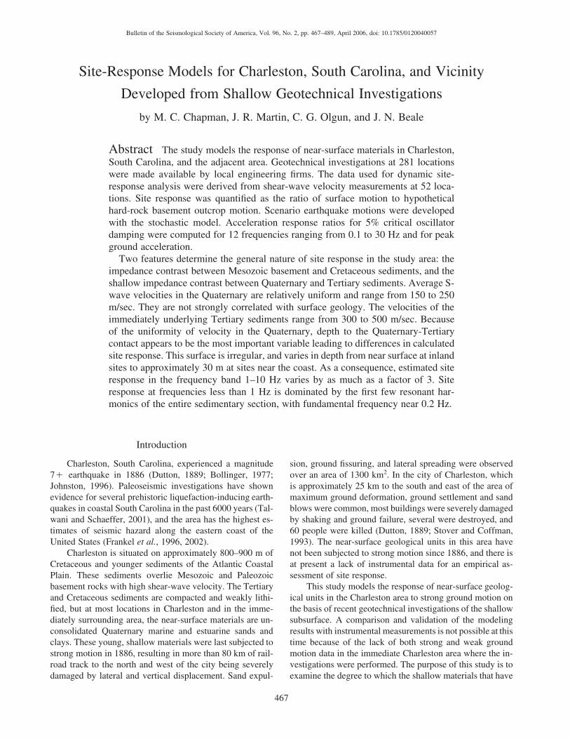
Figure 1 is a geological map of the study area. Table 1gives a brief description of the units present at the surfaceand in the shallow subsurface. The following brief discus-sion is taken from the work of Weems and Lemon (1984,1988, 1993), McCartan et al. (1984), and Weems et al.(1997). Refer to the extensive work of these authors for de-tailed descriptions of lithology, geological profiles, and dis-cussion of the geological history of the study area.

Tertiary Units in the Shallow Subsurface

Tertiary units at shallow depths in the study area arewell compacted and in some cases partially lithified. Theoldest Tertiary units commonly encountered in geotechnicalborings in the shallow subsurface are impermeable lime-stones of the Cooper Group, which includes the EoceneParkers Ferry and overlying Oligocene Ashley formations.The Parker’s Ferry is not exposed at the surface in the studyarea, although both it and the Ashley are ubiquitous in thesubsurface. It is a dense, sticky lime mudstone. The Ashleyformation is a tough phosphatic calcarenite. It is an impor-tant unit for foundation embedment of major construction inthe study area. It resists erosion and is exposed along streambanks in the northwestern section of the study area. Theoverlying Oligocene Chandlers’ Bridge formation is a phos-phatic sand that is easily eroded; exposures are sparse. Ingeneral, the Pliocene Goose Creek Limestone is a soft cal-carenite that is easily eroded, with only very minor exposurein the study area.

Quaternary Units

Quaternary deposits are easily eroded unconsolidatedsediments deposited in back-barrier lagoon, beach-barrier is-land, and shallow marine environments during interglacial

Site-Response Models for Charleston, South Carolina, and Vicinity Developed from Shallow Geotechnical Investigations 469

Figure 1. Geological map of the study area with locations of geotechnical testsshown as filled circles. The geotechnical data include cone penetration tests, seismiccone penetration tests, and standard penetration tests. The geological map is derivedfrom Weems and Lemon (1988, 1993, 1994), McCartan et al. (1984), and Weems etal. (1997). Table 1 lists the geological descriptions of the various mapped units.


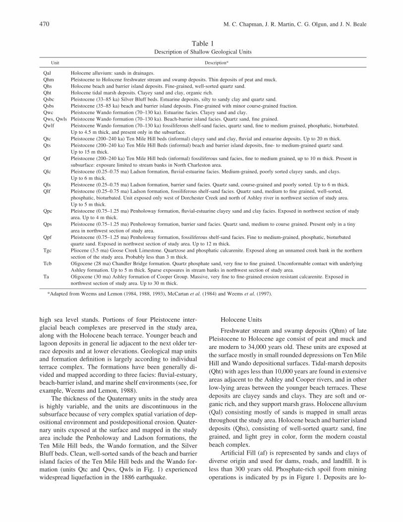
Table 1Description of Shallow Geological Units

Unit Description*

Qal Holocene alluvium: sands in drainages.Qhm Pleistocene to Holocene freshwater stream and swamp deposits. Thin deposits of peat and muck.Qhs Holocene beach and barrier island deposits. Fine-grained, well-sorted quartz sand.Qht Holocene tidal marsh deposits. Clayey sand and clay, organic rich.Qsbc Pleistocene (33–85 ka) Silver Bluff beds. Estuarine deposits, silty to sandy clay and quartz sand.Qsbs Pleistocene (35–85 ka) beach and barrier island deposits. Fine-grained with minor course-grained fraction.Qwc Pleistocene Wando formation (70–130 ka). Estuarine facies. Clayey sand and clay.Qws, Qwls Pleistocene Wando formation (70–130 ka). Beach-barrier island facies. Quartz sand, fine grained.Qwlf Pleistocene Wando formation (70–130 ka) fossiliferous shelf-sand facies, quartz sand, fine to medium grained, phosphatic, bioturbated.

Up to 4.5 m thick, and present only in the subsurface.Qtc Pleistocene (200–240 ka) Ten Mile Hill beds (informal) clayey sand and clay, fluvial and estuarine deposits. Up to 20 m thick.Qts Pleistocene (200–240 ka) Ten Mile Hill Beds (informal) beach and barrier island deposits, fine- to medium-grained quartz sand.

Up to 15 m thick.Qtf Pleistocene (200–240 ka) Ten Mile Hill beds (informal) fossiliferous sand facies, fine to medium grained, up to 10 m thick. Present in

subsurface: exposure limited to stream banks in North Charleston area.Qlc Pleistocene (0.25–0.75 ma) Ladson formation, fluvial-estuarine facies. Medium-grained, poorly sorted clayey sands, and clays.

Up to 6 m thick.Qls Pleistocene (0.25–0.75 ma) Ladson formation, barrier sand facies. Quartz sand, course-grained and poorly sorted. Up to 6 m thick.Qlf Pleistocene (0.25–0.75 ma) Ladson formation, fossiliferous shelf-sand facies. Quartz sand, medium to fine grained, well-sorted,

phosphatic, bioturbated. Unit exposed only west of Dorchester Creek and north of Ashley river in northwest section of study area.Up to 5 m thick.

Qpc Pleistocene (0.75–1.25 ma) Penholoway formation, fluvial-estuarine clayey sand and clay facies. Exposed in northwest section of studyarea. Up to 4 m thick.

Qps Pleistocene (0.75–1.25 ma) Penholoway formation, barrier sand facies. Quartz sand, medium to course grained. Present only in a tinyarea in northwest section of study area.

Qpf Pleistocene (0.75–1.25 ma) Penholoway formation, fossiliferous shelf-sand facies. Fine to medium-grained, phosphatic, bioturbatedquartz sand. Exposed in northwest section of study area. Up to 12 m thick.

Tgc Pliocene (3.5 ma) Goose Creek Limestone. Quartzose and phosphatic calcarenite. Exposed along an unnamed creek bank in the northernsection of the study area. Probably less than 3 m thick.

Tcb Oligocene (28 ma) Chandler Bridge formation. Quartz phosphate sand, very fine to fine grained. Unconformable contact with underlyingAshley formation. Up to 5 m thick. Sparse exposures in stream banks in northwest section of study area.

Ta Oligocene (30 ma) Ashley formation of Cooper Group. Massive, very fine to fine-grained erosion resistant calcarenite. Exposed innorthwest section of study area. Up to 30 m thick.

*Adapted from Weems and Lemon (1984, 1988, 1993), McCartan et al. (1984) and Weems et al. (1997).

high sea level stands. Portions of four Pleistocene inter-glacial beach complexes are preserved in the study area,along with the Holocene beach terrace. Younger beach andlagoon deposits in general lie adjacent to the next older ter-race deposits and at lower elevations. Geological map unitsand formation definition is largely according to individualterrace complex. The formations have been generally di-vided and mapped according to three facies: fluvial-estuary,beach-barrier island, and marine shelf environments (see, forexample, Weems and Lemon, 1988).

The thickness of the Quaternary units in the study areais highly variable, and the units are discontinuous in thesubsurface because of very complex spatial variation of dep-ositional environment and postdepositional erosion. Quater-nary units exposed at the surface and mapped in the studyarea include the Penholoway and Ladson formations, theTen Mile Hill beds, the Wando formation, and the SilverBluff beds. Clean, well-sorted sands of the beach and barrierisland facies of the Ten Mile Hill beds and the Wando for-mation (units Qtc and Qws, Qwls in Fig. 1) experiencedwidespread liquefaction in the 1886 earthquake.

Holocene Units

Freshwater stream and swamp deposits (Qhm) of latePleistocene to Holocene age consist of peat and muck andare modern to 34,000 years old. These units are exposed atthe surface mostly in small rounded depressions on Ten MileHill and Wando depositional surfaces. Tidal-marsh deposits(Qht) with ages less than 10,000 years are found in extensiveareas adjacent to the Ashley and Cooper rivers, and in otherlow-lying areas between the younger beach terraces. Thesedeposits are clayey sands and clays. They are soft and or-ganic rich, and they support marsh grass. Holocene alluvium(Qal) consisting mostly of sands is mapped in small areasthroughout the study area. Holocene beach and barrier islanddeposits (Qhs), consisting of well-sorted quartz sand, finegrained, and light grey in color, form the modern coastalbeach complex.

Artificial Fill (af) is represented by sands and clays ofdiverse origin and used for dams, roads, and landfill. It isless than 300 years old. Phosphate-rich spoil from miningoperations is indicated by ps in Figure 1. Deposits are lo-


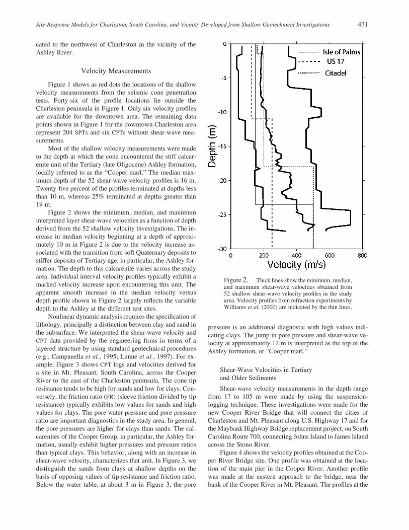
Figure 2. Thick lines show the minimum, median,and maximum shear-wave velocities obtained from52 shallow shear-wave velocity profiles in the studyarea. Velocity profiles from refraction experiments byWilliams et al. (2000) are indicated by the thin lines.

cated to the northwest of Charleston in the vicinity of theAshley River.

Velocity Measurements

Figure 1 shows as red dots the locations of the shallowvelocity measurements from the seismic cone penetrationtests. Forty-six of the profile locations lie outside theCharleston peninsula in Figure 1. Only six velocity profilesare available for the downtown area. The remaining datapoints shown in Figure 1 for the downtown Charleston arearepresent 204 SPTs and six CPTs without shear-wave mea-surements.

Most of the shallow velocity measurements were madeto the depth at which the cone encountered the stiff calcar-enite unit of the Tertiary (late Oligocene) Ashley formation,locally referred to as the “Cooper marl.” The median max-imum depth of the 52 shear-wave velocity profiles is 16 m.Twenty-five percent of the profiles terminated at depths lessthan 10 m, whereas 25% terminated at depths greater than19 m.

Figure 2 shows the minimum, median, and maximuminterpreted layer shear-wave velocities as a function of depthderived from the 52 shallow velocity investigations. The in-crease in median velocity beginning at a depth of approxi-mately 10 m in Figure 2 is due to the velocity increase as-sociated with the transition from soft Quaternary deposits tostiffer deposits of Tertiary age, in particular, the Ashley for-mation. The depth to this calcarenite varies across the studyarea. Individual interval velocity profiles typically exhibit amarked velocity increase upon encountering this unit. Theapparent smooth increase in the median velocity versusdepth profile shown in Figure 2 largely reflects the variabledepth to the Ashley at the different test sites.

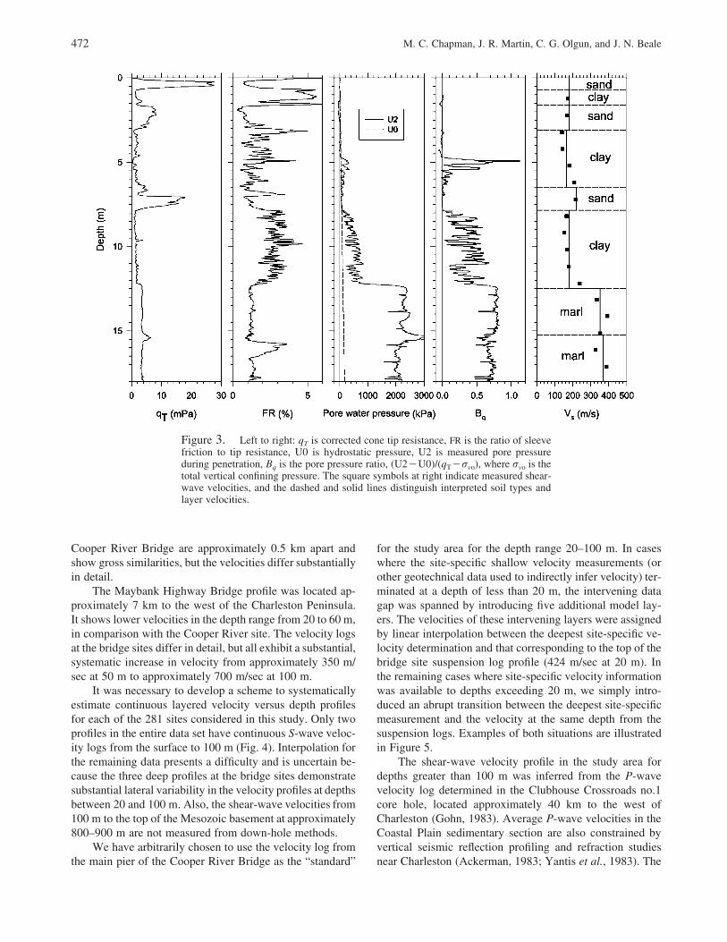
Nonlinear dynamic analysis requires the specification oflithology, principally a distinction between clay and sand inthe subsurface. We interpreted the shear-wave velocity andCPT data provided by the engineering firms in terms of alayered structure by using standard geotechnical procedures(e.g., Campanella et al., 1995; Lunne et al., 1997). For ex-ample, Figure 3 shows CPT logs and velocities derived fora site in Mt. Pleasant, South Carolina, across the CooperRiver to the east of the Charleston peninsula. The cone tipresistance tends to be high for sands and low for clays. Con-versely, the friction ratio (FR) (sleeve friction divided by tipresistance) typically exhibits low values for sands and highvalues for clays. The pore water pressure and pore pressureratio are important diagnostics in the study area. In general,the pore pressures are higher for clays than sands. The cal-carenites of the Cooper Group, in particular, the Ashley for-mation, usually exhibit higher pressures and pressure ratiosthan typical clays. This behavior, along with an increase inshear-wave velocity, characterizes that unit. In Figure 3, wedistinguish the sands from clays at shallow depths on thebasis of opposing values of tip resistance and friction ratio.Below the water table, at about 3 m in Figure 3, the pore

pressure is an additional diagnostic with high values indi-cating clays. The jump in pore pressure and shear-wave ve-locity at approximately 12 m is interpreted as the top of theAshley formation, or “Cooper marl.”

Shear-Wave Velocities in Tertiaryand Older Sediments

Shear-wave velocity measurements in the depth rangefrom 17 to 105 m were made by using the suspension-logging technique. These investigations were made for thenew Cooper River Bridge that will connect the cities ofCharleston and Mt. Pleasant along U.S. Highway 17 and forthe Maybank Highway Bridge replacement project, on SouthCarolina Route 700, connecting Johns Island to James Islandacross the Stono River.

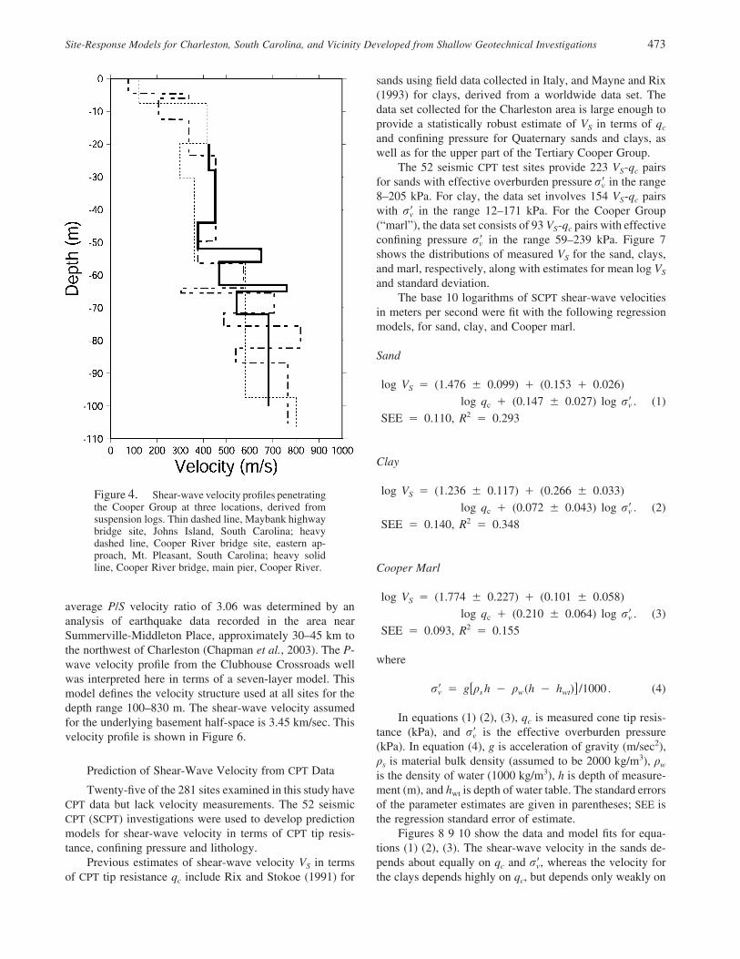
Figure 4 shows the velocity profiles obtained at the Coo-per River Bridge site. One profile was obtained at the loca-tion of the main pier in the Cooper River. Another profilewas made at the eastern approach to the bridge, near thebank of the Cooper River in Mt. Pleasant. The profiles at the


Figure 3. Left to right: qT is corrected cone tip resistance, FR is the ratio of sleevefriction to tip resistance, U0 is hydrostatic pressure, U2 is measured pore pressureduring penetration, Bq is the pore pressure ratio, (U2�U0)/(qT�rvo), where rvo is thetotal vertical confining pressure. The square symbols at right indicate measured shear-wave velocities, and the dashed and solid lines distinguish interpreted soil types andlayer velocities.

Cooper River Bridge are approximately 0.5 km apart andshow gross similarities, but the velocities differ substantiallyin detail.

The Maybank Highway Bridge profile was located ap-proximately 7 km to the west of the Charleston Peninsula.It shows lower velocities in the depth range from 20 to 60 m,in comparison with the Cooper River site. The velocity logsat the bridge sites differ in detail, but all exhibit a substantial,systematic increase in velocity from approximately 350 m/sec at 50 m to approximately 700 m/sec at 100 m.

It was necessary to develop a scheme to systematicallyestimate continuous layered velocity versus depth profilesfor each of the 281 sites considered in this study. Only twoprofiles in the entire data set have continuous S-wave veloc-ity logs from the surface to 100 m (Fig. 4). Interpolation forthe remaining data presents a difficulty and is uncertain be-cause the three deep profiles at the bridge sites demonstratesubstantial lateral variability in the velocity profiles at depthsbetween 20 and 100 m. Also, the shear-wave velocities from100 m to the top of the Mesozoic basement at approximately800–900 m are not measured from down-hole methods.

We have arbitrarily chosen to use the velocity log fromthe main pier of the Cooper River Bridge as the “standard”

for the study area for the depth range 20–100 m. In caseswhere the site-specific shallow velocity measurements (orother geotechnical data used to indirectly infer velocity) ter-minated at a depth of less than 20 m, the intervening datagap was spanned by introducing five additional model lay-ers. The velocities of these intervening layers were assignedby linear interpolation between the deepest site-specific ve-locity determination and that corresponding to the top of thebridge site suspension log profile (424 m/sec at 20 m). Inthe remaining cases where site-specific velocity informationwas available to depths exceeding 20 m, we simply intro-duced an abrupt transition between the deepest site-specificmeasurement and the velocity at the same depth from thesuspension logs. Examples of both situations are illustratedin Figure 5.

The shear-wave velocity profile in the study area fordepths greater than 100 m was inferred from the P-wavevelocity log determined in the Clubhouse Crossroads no.1core hole, located approximately 40 km to the west ofCharleston (Gohn, 1983). Average P-wave velocities in theCoastal Plain sedimentary section are also constrained byvertical seismic reflection profiling and refraction studiesnear Charleston (Ackerman, 1983; Yantis et al., 1983). The


Figure 4. Shear-wave velocity profiles penetratingthe Cooper Group at three locations, derived fromsuspension logs. Thin dashed line, Maybank highwaybridge site, Johns Island, South Carolina; heavydashed line, Cooper River bridge site, eastern ap-proach, Mt. Pleasant, South Carolina; heavy solidline, Cooper River bridge, main pier, Cooper River.

average P/S velocity ratio of 3.06 was determined by ananalysis of earthquake data recorded in the area nearSummerville-Middleton Place, approximately 30–45 km tothe northwest of Charleston (Chapman et al., 2003). The P-wave velocity profile from the Clubhouse Crossroads wellwas interpreted here in terms of a seven-layer model. Thismodel defines the velocity structure used at all sites for thedepth range 100–830 m. The shear-wave velocity assumedfor the underlying basement half-space is 3.45 km/sec. Thisvelocity profile is shown in Figure 6.

Prediction of Shear-Wave Velocity from CPT Data

Twenty-five of the 281 sites examined in this study haveCPT data but lack velocity measurements. The 52 seismicCPT (SCPT) investigations were used to develop predictionmodels for shear-wave velocity in terms of CPT tip resis-tance, confining pressure and lithology.

Previous estimates of shear-wave velocity VS in termsof CPT tip resistance qc include Rix and Stokoe (1991) for

sands using field data collected in Italy, and Mayne and Rix(1993) for clays, derived from a worldwide data set. Thedata set collected for the Charleston area is large enough toprovide a statistically robust estimate of VS in terms of qc

and confining pressure for Quaternary sands and clays, aswell as for the upper part of the Tertiary Cooper Group.

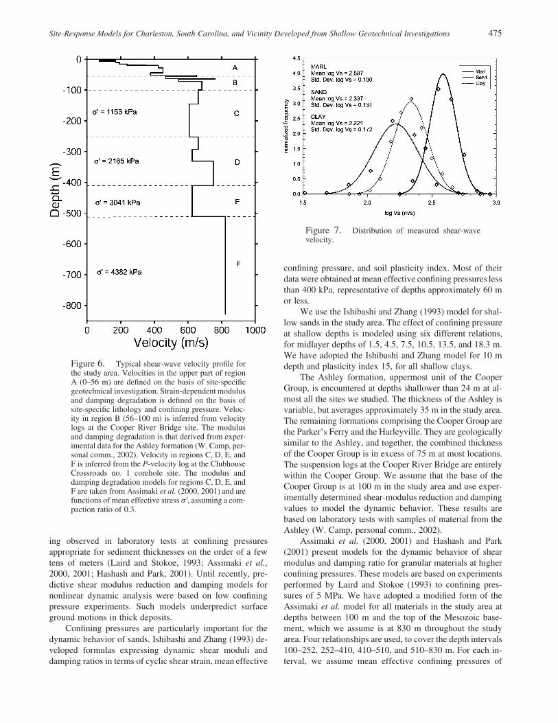
The 52 seismic CPT test sites provide 223 VS-qc pairsfor sands with effective overburden pressure in the ranger�v8–205 kPa. For clay, the data set involves 154 VS-qc pairswith in the range 12–171 kPa. For the Cooper Groupr�v(“marl”), the data set consists of 93 VS-qc pairs with effectiveconfining pressure in the range 59–239 kPa. Figure 7r�vshows the distributions of measured VS for the sand, clays,and marl, respectively, along with estimates for mean log VS

and standard deviation.The base 10 logarithms of SCPT shear-wave velocities

in meters per second were fit with the following regressionmodels, for sand, clay, and Cooper marl.

Sand

log V � (1.476 � 0.099) � (0.153 � 0.026)S

log q � (0.147 � 0.027) log r� . (1)c v2SEE � 0.110, R � 0.293

Clay

log V � (1.236 � 0.117) � (0.266 � 0.033)S

log q � (0.072 � 0.043) log r� . (2)c v2SEE � 0.140, R � 0.348

Cooper Marl

log V � (1.774 � 0.227) � (0.101 � 0.058)S

log q � (0.210 � 0.064) log r� . (3)c v2SEE � 0.093, R � 0.155

where

r� � g[q h � q (h � h )]/1000 . (4)v s w wt

In equations (1) (2), (3), qc is measured cone tip resis-tance (kPa), and is the effective overburden pressurer�v(kPa). In equation (4), g is acceleration of gravity (m/sec2),qs is material bulk density (assumed to be 2000 kg/m3), qw

is the density of water (1000 kg/m3), h is depth of measure-ment (m), and hwt is depth of water table. The standard errorsof the parameter estimates are given in parentheses; SEE isthe regression standard error of estimate.

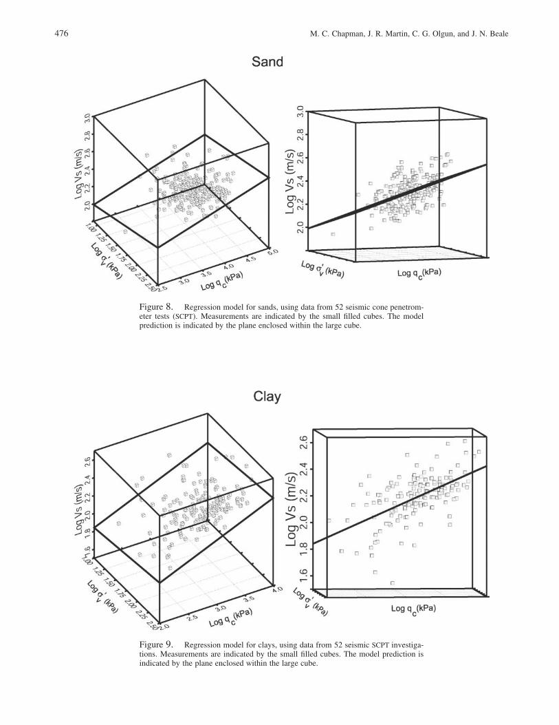
Figures 8 9 10 show the data and model fits for equa-tions (1) (2), (3). The shear-wave velocity in the sands de-pends about equally on qc and , whereas the velocity forr�vthe clays depends highly on qc, but depends only weakly on


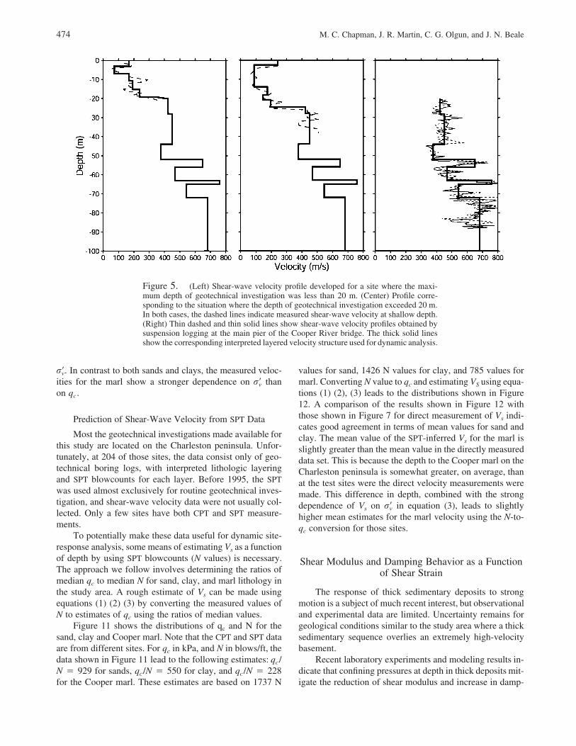
Figure 5. (Left) Shear-wave velocity profile developed for a site where the maxi-mum depth of geotechnical investigation was less than 20 m. (Center) Profile corre-sponding to the situation where the depth of geotechnical investigation exceeded 20 m.In both cases, the dashed lines indicate measured shear-wave velocity at shallow depth.(Right) Thin dashed and thin solid lines show shear-wave velocity profiles obtained bysuspension logging at the main pier of the Cooper River bridge. The thick solid linesshow the corresponding interpreted layered velocity structure used for dynamic analysis.

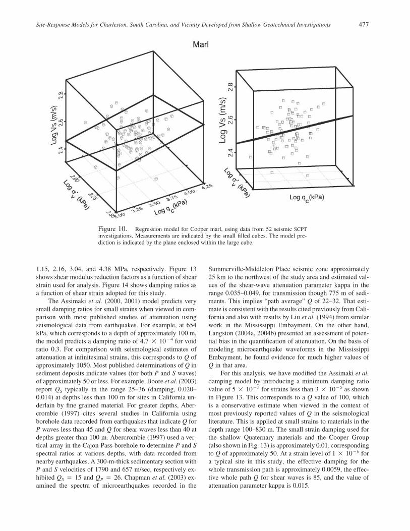
. In contrast to both sands and clays, the measured veloc-r�vities for the marl show a stronger dependence on thanr�von qc.

Prediction of Shear-Wave Velocity from SPT Data

Most the geotechnical investigations made available forthis study are located on the Charleston peninsula. Unfor-tunately, at 204 of those sites, the data consist only of geo-technical boring logs, with interpreted lithologic layeringand SPT blowcounts for each layer. Before 1995, the SPTwas used almost exclusively for routine geotechnical inves-tigation, and shear-wave velocity data were not usually col-lected. Only a few sites have both CPT and SPT measure-ments.

To potentially make these data useful for dynamic site-response analysis, some means of estimating Vs as a functionof depth by using SPT blowcounts (N values) is necessary.The approach we follow involves determining the ratios ofmedian qc to median N for sand, clay, and marl lithology inthe study area. A rough estimate of Vs can be made usingequations (1) (2) (3) by converting the measured values ofN to estimates of qc using the ratios of median values.

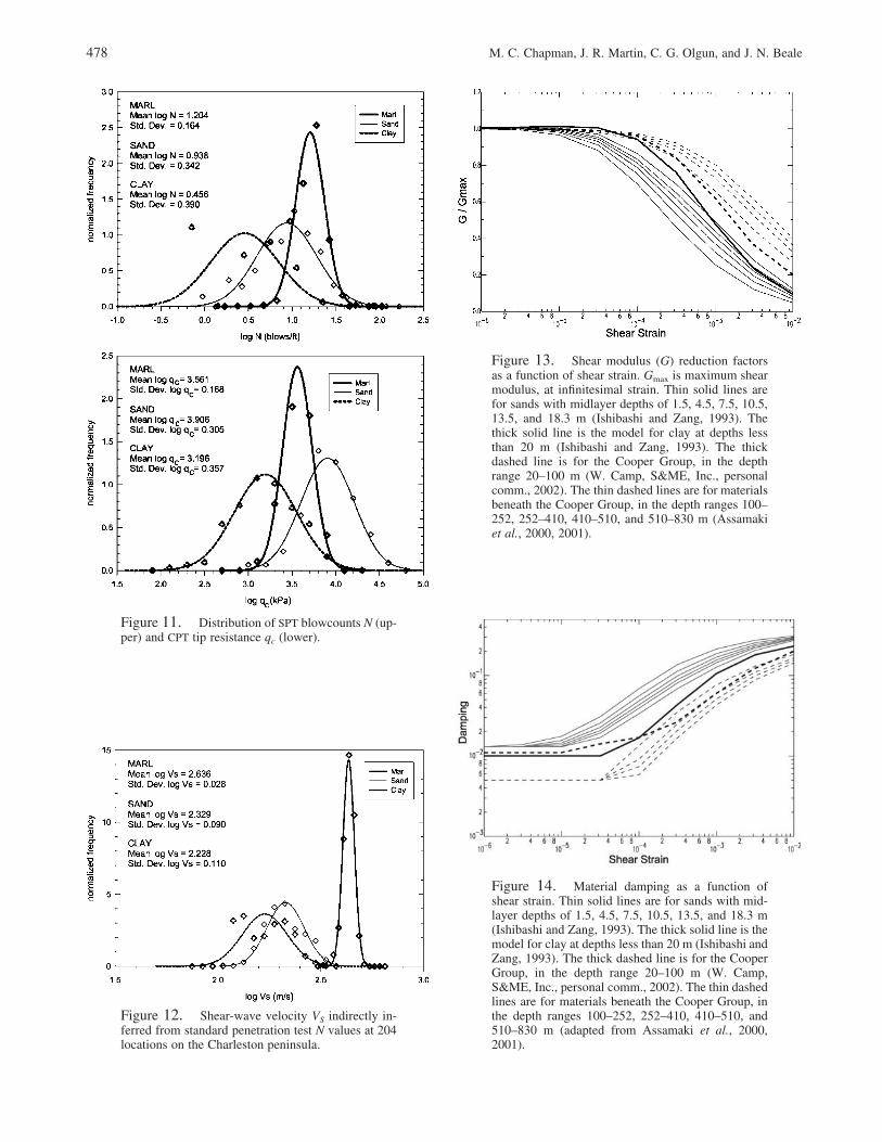
Figure 11 shows the distributions of qc and N for thesand, clay and Cooper marl. Note that the CPT and SPT dataare from different sites. For qc in kPa, and N in blows/ft, thedata shown in Figure 11 lead to the following estimates: qc/N � 929 for sands, qc/N � 550 for clay, and qc/N � 228for the Cooper marl. These estimates are based on 1737 N

values for sand, 1426 N values for clay, and 785 values formarl. Converting N value to qc and estimating VS using equa-tions (1) (2), (3) leads to the distributions shown in Figure12. A comparison of the results shown in Figure 12 withthose shown in Figure 7 for direct measurement of Vs indi-cates good agreement in terms of mean values for sand andclay. The mean value of the SPT-inferred Vs for the marl isslightly greater than the mean value in the directly measureddata set. This is because the depth to the Cooper marl on theCharleston peninsula is somewhat greater, on average, thanat the test sites were the direct velocity measurements weremade. This difference in depth, combined with the strongdependence of Vs on in equation (3), leads to slightlyr�vhigher mean estimates for the marl velocity using the N-to-qc conversion for those sites.

Shear Modulus and Damping Behavior as a Functionof Shear Strain

The response of thick sedimentary deposits to strongmotion is a subject of much recent interest, but observationaland experimental data are limited. Uncertainty remains forgeological conditions similar to the study area where a thicksedimentary sequence overlies an extremely high-velocitybasement.

Recent laboratory experiments and modeling results in-dicate that confining pressures at depth in thick deposits mit-igate the reduction of shear modulus and increase in damp-


Figure 6. Typical shear-wave velocity profile forthe study area. Velocities in the upper part of regionA (0–56 m) are defined on the basis of site-specificgeotechnical investigation. Strain-dependent modulusand damping degradation is defined on the basis ofsite-specific lithology and confining pressure. Veloc-ity in region B (56–100 m) is inferred from velocitylogs at the Cooper River Bridge site. The modulusand damping degradation is that derived from exper-imental data for the Ashley formation (W. Camp, per-sonal comm., 2002). Velocity in regions C, D, E, andF is inferred from the P-velocity log at the ClubhouseCrossroads no. 1 corehole site. The modulus anddamping degradation models for regions C, D, E, andF are taken from Assimaki et al. (2000, 2001) and arefunctions of mean effective stress r�, assuming a com-paction ratio of 0.3.

Figure 7. Distribution of measured shear-wavevelocity.

ing observed in laboratory tests at confining pressuresappropriate for sediment thicknesses on the order of a fewtens of meters (Laird and Stokoe, 1993; Assimaki et al.,2000, 2001; Hashash and Park, 2001). Until recently, pre-dictive shear modulus reduction and damping models fornonlinear dynamic analysis were based on low confiningpressure experiments. Such models underpredict surfaceground motions in thick deposits.

Confining pressures are particularly important for thedynamic behavior of sands. Ishibashi and Zhang (1993) de-veloped formulas expressing dynamic shear moduli anddamping ratios in terms of cyclic shear strain, mean effective

confining pressure, and soil plasticity index. Most of theirdata were obtained at mean effective confining pressures lessthan 400 kPa, representative of depths approximately 60 mor less.

We use the Ishibashi and Zhang (1993) model for shal-low sands in the study area. The effect of confining pressureat shallow depths is modeled using six different relations,for midlayer depths of 1.5, 4.5, 7.5, 10.5, 13.5, and 18.3 m.We have adopted the Ishibashi and Zhang model for 10 mdepth and plasticity index 15, for all shallow clays.

The Ashley formation, uppermost unit of the CooperGroup, is encountered at depths shallower than 24 m at al-most all the sites we studied. The thickness of the Ashley isvariable, but averages approximately 35 m in the study area.The remaining formations comprising the Cooper Group arethe Parker’s Ferry and the Harleyville. They are geologicallysimilar to the Ashley, and together, the combined thicknessof the Cooper Group is in excess of 75 m at most locations.The suspension logs at the Cooper River Bridge are entirelywithin the Cooper Group. We assume that the base of theCooper Group is at 100 m in the study area and use exper-imentally determined shear-modulus reduction and dampingvalues to model the dynamic behavior. These results arebased on laboratory tests with samples of material from theAshley (W. Camp, personal comm., 2002).

Assimaki et al. (2000, 2001) and Hashash and Park(2001) present models for the dynamic behavior of shearmodulus and damping ratio for granular materials at higherconfining pressures. These models are based on experimentsperformed by Laird and Stokoe (1993) to confining pres-sures of 5 MPa. We have adopted a modified form of theAssimaki et al. model for all materials in the study area atdepths between 100 m and the top of the Mesozoic base-ment, which we assume is at 830 m throughout the studyarea. Four relationships are used, to cover the depth intervals100–252, 252–410, 410–510, and 510–830 m. For each in-terval, we assume mean effective confining pressures of


Figure 8. Regression model for sands, using data from 52 seismic cone penetrom-eter tests (SCPT). Measurements are indicated by the small filled cubes. The modelprediction is indicated by the plane enclosed within the large cube.

Figure 9. Regression model for clays, using data from 52 seismic SCPT investiga-tions. Measurements are indicated by the small filled cubes. The model prediction isindicated by the plane enclosed within the large cube.


Figure 10. Regression model for Cooper marl, using data from 52 seismic SCPTinvestigations. Measurements are indicated by the small filled cubes. The model pre-diction is indicated by the plane enclosed within the large cube.

1.15, 2.16, 3.04, and 4.38 MPa, respectively. Figure 13shows shear modulus reduction factors as a function of shearstrain used for analysis. Figure 14 shows damping ratios asa function of shear strain adopted for this study.

The Assimaki et al. (2000, 2001) model predicts verysmall damping ratios for small strains when viewed in com-parison with most published studies of attenuation usingseismological data from earthquakes. For example, at 654kPa, which corresponds to a depth of approximately 100 m,the model predicts a damping ratio of 4.7 � 10�4 for voidratio 0.3. For comparison with seismological estimates ofattenuation at infinitesimal strains, this corresponds to Q ofapproximately 1050. Most published determinations of Q insediment deposits indicate values (for both P and S waves)of approximately 50 or less. For example, Boore et al. (2003)report QS typically in the range 25–36 (damping, 0.020–0.014) at depths less than 100 m for sites in California un-derlain by fine grained material. For greater depths, Aber-crombie (1997) cites several studies in California usingborehole data recorded from earthquakes that indicate Q forP waves less than 45 and Q for shear waves less than 40 atdepths greater than 100 m. Abercrombie (1997) used a ver-tical array in the Cajon Pass borehole to determine P and Sspectral ratios at various depths, with data recorded fromnearby earthquakes. A 300-m-thick sedimentary section withP and S velocities of 1790 and 657 m/sec, respectively ex-hibited QS � 15 and QP � 26. Chapman et al. (2003) ex-amined the spectra of microearthquakes recorded in the

Summerville-Middleton Place seismic zone approximately25 km to the northwest of the study area and estimated val-ues of the shear-wave attenuation parameter kappa in therange 0.035–0.049, for transmission though 775 m of sedi-ments. This implies “path average” Q of 22–32. That esti-mate is consistent with the results cited previously from Cali-fornia and also with results by Liu et al. (1994) from similarwork in the Mississippi Embayment. On the other hand,Langston (2004a, 2004b) presented an assessment of poten-tial bias in the quantification of attenuation. On the basis ofmodeling microearthquake waveforms in the MississippiEmbayment, he found evidence for much higher values ofQ in that area.

For this analysis, we have modified the Assimaki et al.damping model by introducing a minimum damping ratiovalue of 5 � 10�3 for strains less than 3 � 10�5 as shownin Figure 13. This corresponds to a Q value of 100, whichis a conservative estimate when viewed in the context ofmost previously reported values of Q in the seismologicalliterature. This is applied at small strains to materials in thedepth range 100–830 m. The small strain damping used forthe shallow Quaternary materials and the Cooper Group(also shown in Fig. 13) is approximately 0.01, correspondingto Q of approximately 50. At a strain level of 1 � 10�6 fora typical site in this study, the effective damping for thewhole transmission path is approximately 0.0059, the effec-tive whole path Q for shear waves is 85, and the value ofattenuation parameter kappa is 0.015.


Figure 11. Distribution of SPT blowcounts N (up-per) and CPT tip resistance qc (lower).

Figure 13. Shear modulus (G) reduction factorsas a function of shear strain. Gmax is maximum shearmodulus, at infinitesimal strain. Thin solid lines arefor sands with midlayer depths of 1.5, 4.5, 7.5, 10.5,13.5, and 18.3 m (Ishibashi and Zang, 1993). Thethick solid line is the model for clay at depths lessthan 20 m (Ishibashi and Zang, 1993). The thickdashed line is for the Cooper Group, in the depthrange 20–100 m (W. Camp, S&ME, Inc., personalcomm., 2002). The thin dashed lines are for materialsbeneath the Cooper Group, in the depth ranges 100–252, 252–410, 410–510, and 510–830 m (Assamakiet al., 2000, 2001).

Figure 12. Shear-wave velocity VS indirectly in-ferred from standard penetration test N values at 204locations on the Charleston peninsula.

Figure 14. Material damping as a function ofshear strain. Thin solid lines are for sands with mid-layer depths of 1.5, 4.5, 7.5, 10.5, 13.5, and 18.3 m(Ishibashi and Zang, 1993). The thick solid line is themodel for clay at depths less than 20 m (Ishibashi andZang, 1993). The thick dashed line is for the CooperGroup, in the depth range 20–100 m (W. Camp,S&ME, Inc., personal comm., 2002). The thin dashedlines are for materials beneath the Cooper Group, inthe depth ranges 100–252, 252–410, 410–510, and510–830 m (adapted from Assamaki et al., 2000,2001).


Table 2Parameters of the Stochastic Model Used to Generate Basement

Outcrop Motion for Dynamic Response Analysis

Epicentral distance: 30 kmFocal depth: 10 kmCrustal velocity: 3.5 km/secCrustal density: 2.6 g/cm3

Stress parameter: 100 barsCrustal quality factor: Q � 680 f 0.36

Free surface factor: 2.0Radiation pattern: 0.55Component partition factor: 0.707

Moment Magnitude Mean PGA* (g) Scaling Factor†

6.4 0.169 0.591 for 0.1g6.7 0.218 0.917 for 0.2g7.1 0.300 1.000 for 0.3g7.5 0.436 0.917 for 0.4g7.5 0.436 1.147 for 0.5g7.5 0.436 1.376 for 0.6g

*Mean PGA from 20 realizations of the stochastic model.†Scaling factor applied to each of 20 simulations for use in response

analysis.

Response Estimates

Input Ground Motions

We use five different levels of input motion intensity tomodel the nonlinear response of the sedimentary section inthe study area. The motions are distinguished by peak ac-celeration values.

A point-source stochastic model (e.g., Boore, 1983;Boore and Atkinson, 1987; Atkinson and Boore, 1995) wasused to simulate the outcrop motions of pre-Cretaceous base-ment rock. Table 2 lists the parameters of the stochasticmodel used to make the simulations. The scenario earth-quake in all cases is at an epicentral distance of 30 km, andat a depth of 10 km. This scenario is consistent with a sourcein the area of maximum shaking intensity in 1886, centeredapproximately 30 km to the northwest of Charleston in thevicinity of Summerville (Dutton, 1889). The motions gen-erated for 0.1, 0.2, and 0.3g peak acceleration are simulatedby using moment magnitude M 6.4, 6.7, and 7.1, respec-tively. The upper range of estimates of the moment magni-tude of the 1886 earthquake is 7.5 (Johnston, 1996). We usedM 7.5 to generate the time series for the 0.4 and 0.5g accel-eration levels.

Twenty acceleration time series were simulated for eachpeak ground acceleration (PGA) level. Because PGA is a ran-dom variable, the PGA value for each realization of the sto-chastic model varies slightly. To ensure that the target PGAlevel was accurately represented, we estimated the meanPGA for the 20 simulations at each magnitude level. The 20time series were then scaled such that the mean peak accel-eration of the 20 simulations was equal to the desired meanpeak acceleration value. The 20 time series were then usedto develop mean estimates of the ratios of spectral acceler-

ation (SA) response on the ground surface to that of the SAresponse on an outcrop of the basement rock at each studysite.

Site Conditions and General Site-ResponseCharacteristics

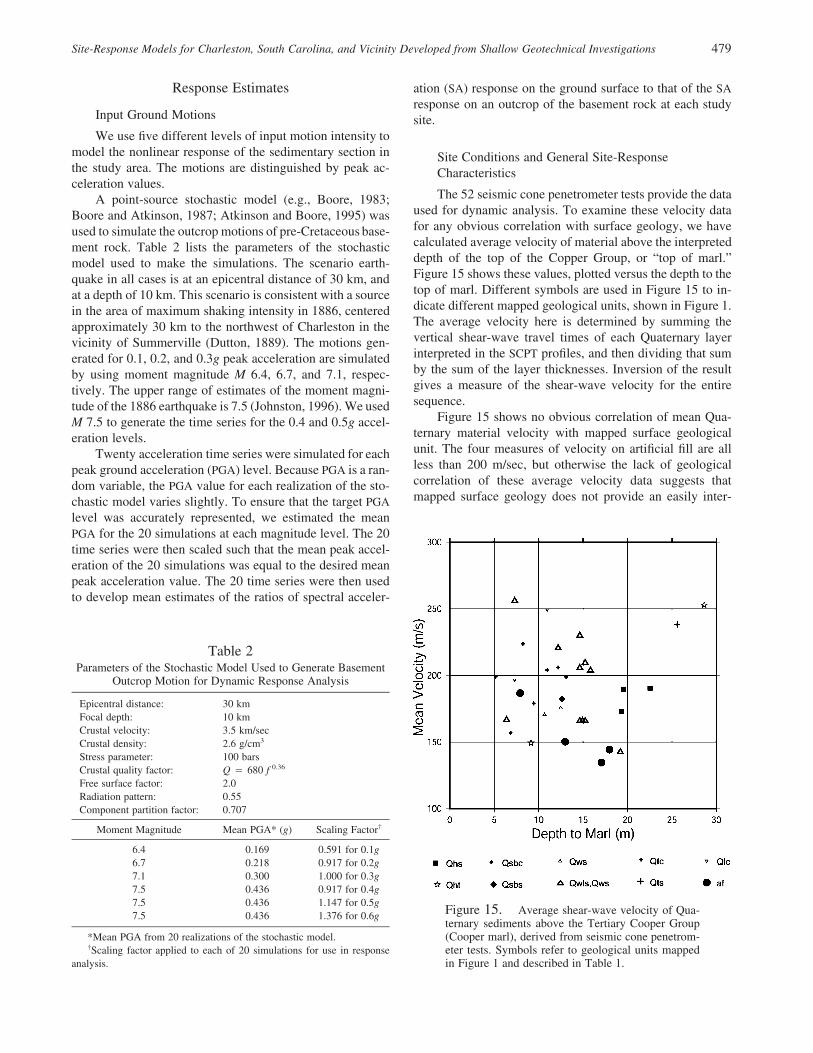
The 52 seismic cone penetrometer tests provide the dataused for dynamic analysis. To examine these velocity datafor any obvious correlation with surface geology, we havecalculated average velocity of material above the interpreteddepth of the top of the Copper Group, or “top of marl.”Figure 15 shows these values, plotted versus the depth to thetop of marl. Different symbols are used in Figure 15 to in-dicate different mapped geological units, shown in Figure 1.The average velocity here is determined by summing thevertical shear-wave travel times of each Quaternary layerinterpreted in the SCPT profiles, and then dividing that sumby the sum of the layer thicknesses. Inversion of the resultgives a measure of the shear-wave velocity for the entiresequence.

Figure 15 shows no obvious correlation of mean Qua-ternary material velocity with mapped surface geologicalunit. The four measures of velocity on artificial fill are allless than 200 m/sec, but otherwise the lack of geologicalcorrelation of these average velocity data suggests thatmapped surface geology does not provide an easily inter-

Figure 15. Average shear-wave velocity of Qua-ternary sediments above the Tertiary Cooper Group(Cooper marl), derived from seismic cone penetrom-eter tests. Symbols refer to geological units mappedin Figure 1 and described in Table 1.


preted diagnostic for potential variation of mean Quaternarymaterial velocity. Although the measured shear-wave veloc-ity data set is very small for most of the individual units, thevelocities for the Quaternary as a whole appear to clustertightly about a central value of 200 m/sec, suggesting thatas a whole, the sediments are relatively uniform in terms ofshear moduli.

The small range of variation of mean velocity (� 50m/sec) about a central value of 200 m/sec has implicationsfor site-response prediction. The vertical time of shear-wavepropagation through the Quaternary section at these sitesdepends largely on the variable thickness of the section be-cause the site-to-site variation of velocity in the Quaternarysediments is small. For example, Figure 15 shows that thisthickness varies between about 5 and 30 m for the 52 SCPTsites with measured shear-wave velocity data.

Although there is no clear correlation of Quaternary av-erage velocity and mapped surface geology based on the the52 seismic cone penetrometer tests, there is a correlation ofdepth to the Tertiary units (marl) and mapped surface ge-ology. In general, Tertiary units are near the surface in thenorthern and northwestern parts of the study area and areexposed in stream banks in those areas. The Tertiary unitslie at greater depths beneath the progressively younger beachterrace complexes that roughly parallel the coastline. Hence,Quaternary sediments of the Ladson formation (Qlc) are rela-tively thin in the northwestern section of the study area,whereas sites on the younger Ten Mile Hill beds typicallyoverlie a somewhat deeper Tertiary-Quaternary contact, andsites in the Wando, Silver Bluff, and modern terrace complex,in general, overlie the Tertiary units at still greater depths.Although depth to Tertiary is correlated with the age of thesurface deposits, this correlation is weak because the Tertiary-Quaternary contact is an irregular surface. Depth to that sur-face depends on ground surface elevation, as well as the com-plex erosion and depositional history of the study area.

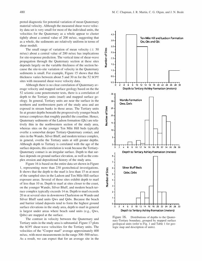
Figure 16 is based on the entire data set shown in Figure1, representing more than 230 geotechnical investigations.It shows that the depth to the marl is less than 15 m at mostof the sampled sites in the Ladson and Ten Mile Hill surfaceexposure areas. Several of those sites exhibit depth to marlof less than 10 m. Depth to marl at sites closer to the coast,on the younger Wando, Silver Bluff, and modern beach ter-race complex typically exceeds 14 m. Depth to marl exceeds20 m at several sites in downtown Charleston on Wando andSilver Bluff sand units Qws and Qsbs. Because the beachand barrier island deposits tend to form the highest groundsurface elevations in the study area, depth to marl in generalis largest under areas where beach sand units (e.g., Qws,Qsbs) are mapped at the surface.

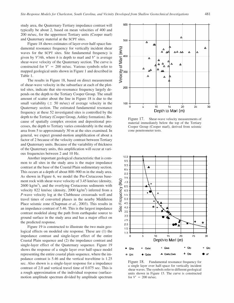
The contrast in velocity between the Quaternary andTertiary units in the study area is substantial. Figure 17 plotsthe SCPT shear-wave velocities for the Tertiary units. Thevelocities of the “Cooper marl” average approximately 400m/sec, with most measurements in the range 300–500 m/sec.As a result, we can expect that for an average site in the

Figure 16. Distributions of depths to the Quater-nary-Tertiary boundary, grouped by mapped surfacegeological units (refer to Fig. 1 and Table 1 for geo-logic map and description of units).


Figure 17. Shear-wave velocity measurements ofmaterial immediately below the top of the TertiaryCooper Group (Cooper marl), derived from seismiccone penetrometer tests.

Figure 18. Fundamental resonance frequency fora single layer over half-space for vertically incidentshear waves. The symbols refer to different geologicalunits shown in Figure 15. The curve is constructedfor V� � 200 m/sec.

study area, the Quaternary-Tertiary impedance contrast willtypically be about 2, based on mean velocities of 400 and200 m/sec, for the uppermost Tertiary units (Cooper marl)and Quaternary material at the SCPT sites.

Figure 18 shows estimates of layer-over-half-space fun-damental resonance frequency for vertically incident shearwaves for the SCPT sites. Site fundamental frequency isgiven by V�/4h, where h is depth to marl and V� is averageshear-wave velocity of the Quaternary section. The curve isconstructed for V� � 200 m/sec. Various symbols refer tomapped geological units shown in Figure 1 and described inTable 1.

The results in Figure 18, based on direct measurementof shear-wave velocity in the subsurface at each of the plot-ted sites, indicate that site-resonance frequency largely de-pends on the depth to the Tertiary Cooper Group. The smallamount of scatter about the line in Figure 18 is due to thesmall variability (� 50 m/sec) of average velocity in theQuaternary section. The estimated fundamental resonancefrequency at these 52 investigated sites is controlled by thedepth to the Tertiary (Cooper Group, Ashley formation). Be-cause of spatially complex erosion and depositional pro-cesses, the depth to Tertiary varies considerably in the studyarea from 5 to approximately 30 m at the sites examined. Ingeneral, we expect ground-motion amplification of about afactor of 2 because of the velocity contrast between Tertiaryand Quaternary units. Because of the variability of thicknessof the Quaternary units, this amplification will occur at vari-ous frequencies between 2 and 10 Hz.

Another important geological characteristic that is com-mon to all sites in the study area is the major impedancecontrast at the base of the Coastal Plain sedimentary section.This occurs at a depth of about 800–900 m in the study area.As shown in Figure 6, we model the Pre-Cretaceous base-ment rock with shear-wave velocity of 3.45 km/sec (density,2600 kg/m3), and the overlying Cretaceous sediments withvelocity 822 km/sec (density, 2000 kg/m3) inferred from aP-wave velocity log at the Clubhouse crossroads well andtravel times of converted phases in the nearby MiddletonPlace seismic zone (Chapman et al., 2003). This results inan impedance contrast of 5.46. This is the largest impedancecontrast modeled along the path from earthquake source toground surface in the study area and has a major effect onthe predicted response.

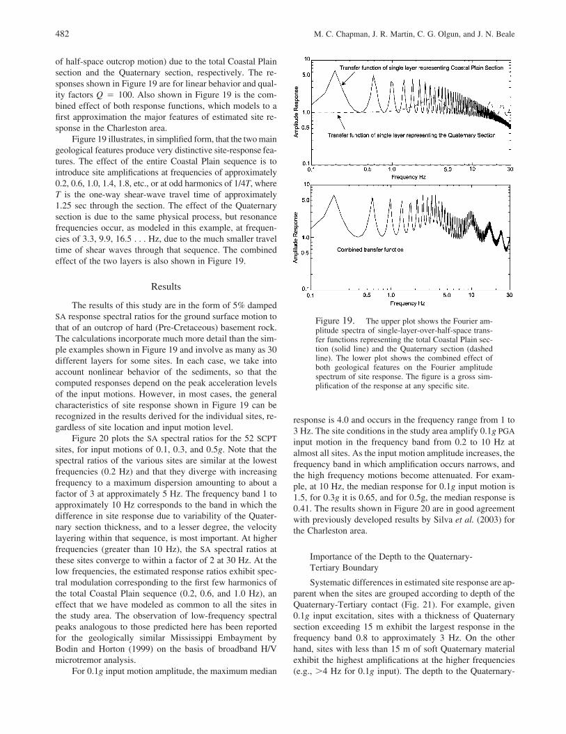
Figure 19 is constructed to illustrate the two main geo-logical effects on modeled site response. These are (1) theimpedance contrast and single-layer effect of the entireCoastal Plain sequence and (2) the impedance contrast andsingle-layer effect of the Quaternary sequence. Figure 19shows the response of a single layer over half-space modelrepresenting the entire coastal plain sequence, where the im-pedance contrast is 5.46 and the vertical traveltime is 1.25sec. Also shown is a single-layer response for a impedancecontrast of 2.0 and vertical travel time of 0.075 sec. This isa rough approximation of the individual response (surface-motion amplitude spectrum divided by amplitude spectrum


Figure 19. The upper plot shows the Fourier am-plitude spectra of single-layer-over-half-space trans-fer functions representing the total Coastal Plain sec-tion (solid line) and the Quaternary section (dashedline). The lower plot shows the combined effect ofboth geological features on the Fourier amplitudespectrum of site response. The figure is a gross sim-plification of the response at any specific site.

of half-space outcrop motion) due to the total Coastal Plainsection and the Quaternary section, respectively. The re-sponses shown in Figure 19 are for linear behavior and qual-ity factors Q � 100. Also shown in Figure 19 is the com-bined effect of both response functions, which models to afirst approximation the major features of estimated site re-sponse in the Charleston area.

Figure 19 illustrates, in simplified form, that the two maingeological features produce very distinctive site-response fea-tures. The effect of the entire Coastal Plain sequence is tointroduce site amplifications at frequencies of approximately0.2, 0.6, 1.0, 1.4, 1.8, etc., or at odd harmonics of 1/4T, whereT is the one-way shear-wave travel time of approximately1.25 sec through the section. The effect of the Quaternarysection is due to the same physical process, but resonancefrequencies occur, as modeled in this example, at frequen-cies of 3.3, 9.9, 16.5 . . . Hz, due to the much smaller traveltime of shear waves through that sequence. The combinedeffect of the two layers is also shown in Figure 19.

Results

The results of this study are in the form of 5% dampedSA response spectral ratios for the ground surface motion tothat of an outcrop of hard (Pre-Cretaceous) basement rock.The calculations incorporate much more detail than the sim-ple examples shown in Figure 19 and involve as many as 30different layers for some sites. In each case, we take intoaccount nonlinear behavior of the sediments, so that thecomputed responses depend on the peak acceleration levelsof the input motions. However, in most cases, the generalcharacteristics of site response shown in Figure 19 can berecognized in the results derived for the individual sites, re-gardless of site location and input motion level.

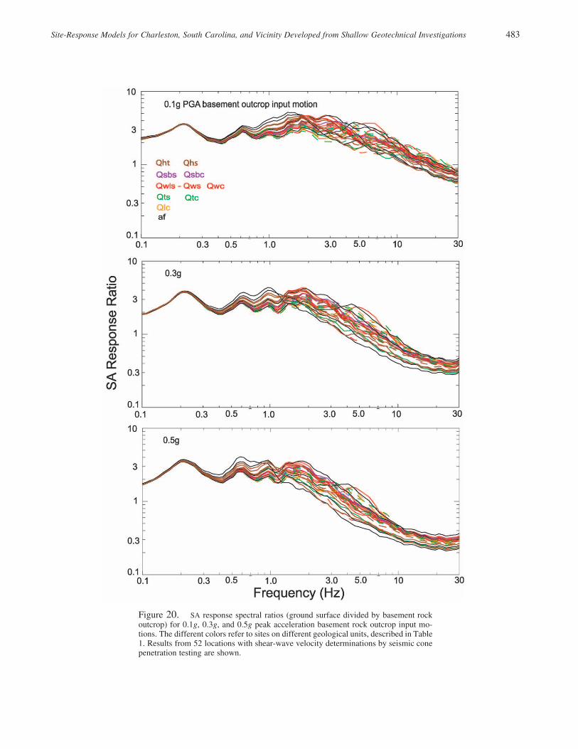
Figure 20 plots the SA spectral ratios for the 52 SCPTsites, for input motions of 0.1, 0.3, and 0.5g. Note that thespectral ratios of the various sites are similar at the lowestfrequencies (0.2 Hz) and that they diverge with increasingfrequency to a maximum dispersion amounting to about afactor of 3 at approximately 5 Hz. The frequency band 1 toapproximately 10 Hz corresponds to the band in which thedifference in site response due to variability of the Quater-nary section thickness, and to a lesser degree, the velocitylayering within that sequence, is most important. At higherfrequencies (greater than 10 Hz), the SA spectral ratios atthese sites converge to within a factor of 2 at 30 Hz. At thelow frequencies, the estimated response ratios exhibit spec-tral modulation corresponding to the first few harmonics ofthe total Coastal Plain sequence (0.2, 0.6, and 1.0 Hz), aneffect that we have modeled as common to all the sites inthe study area. The observation of low-frequency spectralpeaks analogous to those predicted here has been reportedfor the geologically similar Mississippi Embayment byBodin and Horton (1999) on the basis of broadband H/Vmicrotremor analysis.

For 0.1g input motion amplitude, the maximum median

response is 4.0 and occurs in the frequency range from 1 to3 Hz. The site conditions in the study area amplify 0.1g PGAinput motion in the frequency band from 0.2 to 10 Hz atalmost all sites. As the input motion amplitude increases, thefrequency band in which amplification occurs narrows, andthe high frequency motions become attenuated. For exam-ple, at 10 Hz, the median response for 0.1g input motion is1.5, for 0.3g it is 0.65, and for 0.5g, the median response is0.41. The results shown in Figure 20 are in good agreementwith previously developed results by Silva et al. (2003) forthe Charleston area.

Importance of the Depth to the Quaternary-Tertiary Boundary

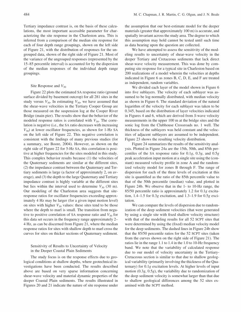
Systematic differences in estimated site response are ap-parent when the sites are grouped according to depth of theQuaternary-Tertiary contact (Fig. 21). For example, given0.1g input excitation, sites with a thickness of Quaternarysection exceeding 15 m exhibit the largest response in thefrequency band 0.8 to approximately 3 Hz. On the otherhand, sites with less than 15 m of soft Quaternary materialexhibit the highest amplifications at the higher frequencies(e.g., �4 Hz for 0.1g input). The depth to the Quaternary-


Figure 20. SA response spectral ratios (ground surface divided by basement rockoutcrop) for 0.1g, 0.3g, and 0.5g peak acceleration basement rock outcrop input mo-tions. The different colors refer to sites on different geological units, described in Table1. Results from 52 locations with shear-wave velocity determinations by seismic conepenetration testing are shown.


Tertiary impedance contrast is, on the basis of these calcu-lations, the most important accessible parameter for char-acterizing the site response in the Charleston area. This isinferred from a comparison of the median site response foreach of four depth range groupings, shown on the left sideof Figure 21, with the distribution of responses for the un-grouped data, shown of the right side of Figure 21. Most ofthe variance of the ungrouped responses (represented by the15–85 percentile interval) is accounted for by the dispersionof the median responses of the individual depth rangegroupings.

Site Response and V30

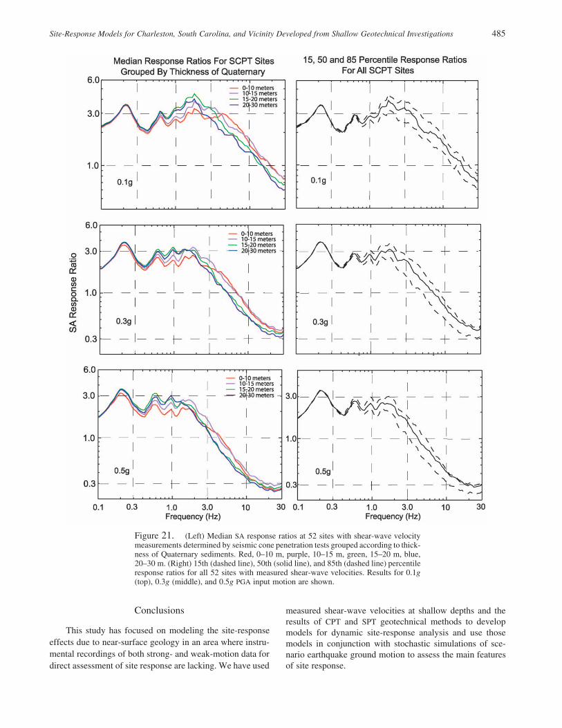
Figure 22 plots the estimated SA response ratio (groundsurface divided by basement outcrop) for all 281 sites in thestudy versus V30. In estimating V30, we have assumed thatthe shear-wave velocities in the Tertiary Cooper Group arethose measured on the suspension log at the Cooper RiverBridge (main pier). The results show that the behavior of themodeled response ratios is correlated with V30. The corre-lation is negative (i.e., the SA ratio decreases with increasingV30) at lower oscillator frequencies, as shown for 1-Hz SAon the left side of Figure 22. This negative correlation isconsistent with the findings of many previous studies (fora summary, see Boore, 2004). However, as shown on theright side of Figure 22 for 5-Hz SA, this correlation is posi-tive at higher frequencies for the sites modeled in this study.This complex behavior results because (1) the velocities ofthe Quaternary sediments are similar at the different sites,(2) the impedance contrast between the Quaternary and Ter-tiary sediments is large (a factor of approximately 2, on av-erage), and (3) the depth to the large Quaternary and Tertiaryimpedance contrast is highly variable at the different sitesbut lies within the interval used to determine V30 (30 m).Our modeling of the Charleston area suggests that site-response ratios for oscillator frequencies exceeding approx-imately 4 Hz may be larger (for a given input motion level)on sites with higher V30 values: these sites tend to be thosewhere the depth to marl is small. The transition from nega-tive to positive correlation of SA response ratio and V30 forthis data set occurs in the frequency range approximately 2–4 Hz, as can be discerned from Figure 21, where the medianresponse ratios for sites with shallow depth to marl cross thecurves for sites on thicker sections of Quaternary sediment.

Sensitivity of Results to Uncertainty of Velocityin the Deeper Coastal Plain Sediments

The study focus is on the response effects due to geo-logical conditions at shallow depths, where geotechnical in-vestigations have been conducted. The results describedabove are based on very sparse information concerningshear-wave velocity and material dynamic properties of thedeeper Coastal Plain sediments. The results illustrated inFigures 20 and 21 indicate the nature of site response under

the assumption that our best-estimate model for the deepermaterials (greater that approximately 100 m) is accurate, andspatially invariant across the study area. The degree to whichthis assumption may hold cannot be tested until such timeas data bearing upon the question are collected.

We have attempted to assess the sensitivity of the mod-eling results to uncertainty of shear-wave velocity in thedeeper Tertiary and Cretaceous sediments that lack directshear-wave velocity measurement. This was done by com-puting site response for a typical site in Charleston based on200 realizations of a model wherein the velocities at depthsindicated in Figure 6 as zones B, C, D, E, and F are treatedas independent, random variables.

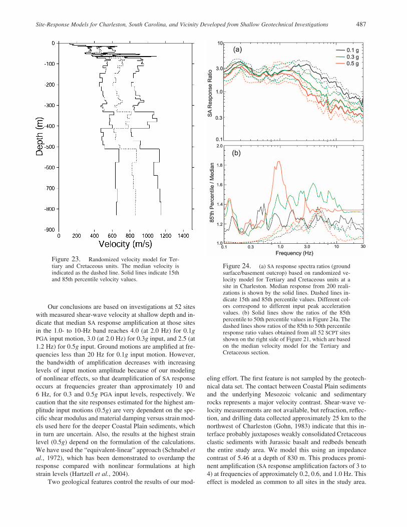
We divided each layer of the model shown in Figure 6into five sublayers. The velocity of each sublayer was as-sumed to be log-normally distributed, with median velocityas shown in Figure 6. The standard deviation of the naturallogarithm of the velocity for each sublayer was taken to be0.345, based on the distribution of layer velocities indicatedin Figures 4 and 6, which are derived from S-wave velocitymeasurements in the upper 100 m at the bridge sites and thesonic log from the Clubhouse Crossroads no. 1 well. Thethickness of the sublayers was held constant and the veloc-ities of adjacent sublayers are assumed to be independent.Figure 23 shows the resulting velocity distribution.

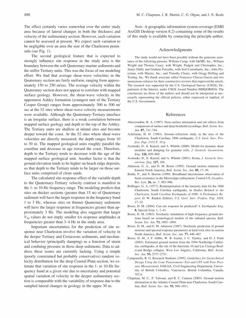
Figure 24 summarizes the results of the sensitivity anal-ysis. Plotted in Figure 24a are the 15th, 50th, and 85th per-centiles of the SA response ratio for 0.1g, 0.3g, and 0.5gpeak acceleration input motion at a single site using the (con-stant) measured velocity profile in zone A and the random-ized velocity model for zones B through F. The range ofdispersion for each of the three levels of excitation at thissite is quantified as the ratio of the 85th percentile value tothat of the 50th percentile (median) value, and plotted inFigure 24b. We observe that in the 1- to 10-Hz range, the85/50 percentile ratio is approximately 1.2 for 0.1g excita-tion, 1.4–1.5 for 0.3g excitation, and 1.3–1.9 for 0.5g exci-tation.

We can compare the levels of dispersion due to random-ization of the deep sediment velocities (that were generatedby using a single site with fixed shallow velocity structure)with that of the modeling results for all 52 SCPT sites thatwere determined by using the (fixed) median velocity modelfor the deep sediments. The dashed lines in Figure 24b showthat the 85/50 percentile ratios for the 52 SCPT sites (takenfrom the curves shown on the right side of Figure 21). Theratios lie in the range 1.1 to 1.4 in the 1.0 to 10-Hz frequencyband. We note that the variability of calculated responsedue to our model of velocity uncertainty in the Tertiary-Cretaceous section is similar to that due to shallow geolog-ical variability (primarily involving the thickness of the Qua-ternary) for 0.1g excitation levels. At higher levels of inputmotion (0.3g, 0.5g), the variability due to randomization ofthe deep sediment velocity is somewhat larger than that dueto shallow geological differences among the 52 sites ex-amined with the SCPT method.


Figure 21. (Left) Median SA response ratios at 52 sites with shear-wave velocitymeasurements determined by seismic cone penetration tests grouped according to thick-ness of Quaternary sediments. Red, 0–10 m, purple, 10–15 m, green, 15–20 m, blue,20–30 m. (Right) 15th (dashed line), 50th (solid line), and 85th (dashed line) percentileresponse ratios for all 52 sites with measured shear-wave velocities. Results for 0.1g(top), 0.3g (middle), and 0.5g PGA input motion are shown.

Conclusions

This study has focused on modeling the site-responseeffects due to near-surface geology in an area where instru-mental recordings of both strong- and weak-motion data fordirect assessment of site response are lacking. We have used

measured shear-wave velocities at shallow depths and theresults of CPT and SPT geotechnical methods to developmodels for dynamic site-response analysis and use thosemodels in conjunction with stochastic simulations of sce-nario earthquake ground motion to assess the main featuresof site response.


Figure 22. Modeled SA response ratios at 281 study sites (ground surface dividedby basement rock outcrop) versus average velocity in the upper 30 m for 1 Hz (left)and 5 Hz (right). The plots are constructed for basement rock outcrop input motion of0.1g (top), 0.3g (middle), and 0.5g (bottom) PGA.


Figure 23. Randomized velocity model for Ter-tiary and Cretaceous units. The median velocity isindicated as the dashed line. Solid lines indicate 15thand 85th percentile velocity values.

Figure 24. (a) SA response spectra ratios (groundsurface/basement outcrop) based on randomized ve-locity model for Tertiary and Cretaceous units at asite in Charleston. Median response from 200 reali-zations is shown by the solid lines. Dashed lines in-dicate 15th and 85th percentile values. Different col-ors correspond to different input peak accelerationvalues. (b) Solid lines show the ratios of the 85thpercentile to 50th percentile values in Figure 24a. Thedashed lines show ratios of the 85th to 50th percentileresponse ratio values obtained from all 52 SCPT sitesshown on the right side of Figure 21, which are basedon the median velocity model for the Tertiary andCretaceous section.

Our conclusions are based on investigations at 52 siteswith measured shear-wave velocity at shallow depth and in-dicate that median SA response amplification at those sitesin the 1.0- to 10-Hz band reaches 4.0 (at 2.0 Hz) for 0.1gPGA input motion, 3.0 (at 2.0 Hz) for 0.3g input, and 2.5 (at1.2 Hz) for 0.5g input. Ground motions are amplified at fre-quencies less than 20 Hz for 0.1g input motion. However,the bandwidth of amplification decreases with increasinglevels of input motion amplitude because of our modelingof nonlinear effects, so that deamplification of SA responseoccurs at frequencies greater than approximately 10 and6 Hz, for 0.3 and 0.5g PGA input levels, respectively. Wecaution that the site responses estimated for the highest am-plitude input motions (0.5g) are very dependent on the spe-cific shear modulus and material damping versus strain mod-els used here for the deeper Coastal Plain sediments, whichin turn are uncertain. Also, the results at the highest strainlevel (0.5g) depend on the formulation of the calculations.We have used the “equivalent-linear” approach (Schnabel etal., 1972), which has been demonstrated to overdamp theresponse compared with nonlinear formulations at highstrain levels (Hartzell et al., 2004).

Two geological features control the results of our mod-

eling effort. The first feature is not sampled by the geotech-nical data set. The contact between Coastal Plain sedimentsand the underlying Mesozoic volcanic and sedimentaryrocks represents a major velocity contrast. Shear-wave ve-locity measurements are not available, but refraction, reflec-tion, and drilling data collected approximately 25 km to thenorthwest of Charleston (Gohn, 1983) indicate that this in-terface probably juxtaposes weakly consolidated Cretaceousclastic sediments with Jurassic basalt and redbeds beneaththe entire study area. We model this using an impedancecontrast of 5.46 at a depth of 830 m. This produces promi-nent amplification (SA response amplification factors of 3 to4) at frequencies of approximately 0.2, 0.6, and 1.0 Hz. Thiseffect is modeled as common to all sites in the study area.


The effect certainly varies somewhat over the entire studyarea because of lateral changes in both the thickness andvelocity of the sedimentary section. However, such variationcannot be assessed at present. We expect such variation tobe negligible over an area the size of the Charleston penin-sula (see Fig. 1).

The second geological feature that is expected tostrongly influence site response in the study area is theboundary between the soft Quaternary marine sediments andthe stiffer Tertiary units. This was the focus of our modelingeffort. We find that average shear-wave velocities in theQuaternary section are fairly uniform, ranging from approx-imately 150 to 250 m/sec. The average velocity within theQuaternary section does not appear to correlate with mappedsurface geology. However, the shear-wave velocity in theuppermost Ashley formation (youngest unit of the TertiaryCooper Group) ranges from approximately 300 to 500 m/sec at the 52 sites where shear-wave velocity measurementswere available. Although the Quaternary-Tertiary interfaceis an irregular surface, there is a weak correlation betweenmapped surface geology and depth to the top of the Ashley.The Tertiary units are shallow at inland sites and becomedeeper toward the coast. At the 52 sites where shear-wavevelocities are directly measured, the depth ranges from 10to 30 m. The mapped geological units roughly parallel thecoastline and decrease in age toward the coast. Therefore,depth to the Tertiary tends to decrease with the age of themapped surface geological unit. Another factor is that theground elevation tends to be higher on beach ridge deposits,so that depth to the Tertiary tends to be larger on those sur-face units comprised of clean sands.

The calculated site-response effect of the variable depthto the Quaternary-Tertiary velocity contrast is manifest inthe 1- to 10-Hz frequency range. The modeling predicts thatsites on thicker sections (greater than 15 m) of Quaternarysediment will have the larger response in the frequency band1 to 3 Hz, whereas sites on thinner Quaternary sedimentswill have the larger response at frequencies greater than ap-proximately 3 Hz. The modeling also suggests that largerV30 values do not imply smaller SA response amplitudes atfrequencies greater than 3–4 Hz in the study area.

Important uncertainties for the prediction of site re-sponse near Charleston involve the variation of velocity inthe deeper Tertiary and Cretaceous sediments, and mechan-ical behavior (principally damping) as a function of strainand confining pressure in those deep sediments. Data to ad-dress these issues are currently lacking. Using a simple(poorly constrained but probably conservative) random ve-locity distribution for the deep Coastal Plain section, we es-timate that variation of site response in the 1- to 10-Hz fre-quency band at a given site due to uncertainty and potentialspatial variation of velocity in the deeper sedimentary sec-tion is comparable with the variability of response due to thesampled lateral changes in geology in the upper 30 m.

Note: A geographic information system coverage (ESRIArcGIS Desktop version 8.2) containing some of the resultsof this study is available by contacting the principle author.

Acknowledgments

The study would not have been possible without the generous assis-tance of the following persons: William Camp, with S&ME, Inc.; WilliamWright and Thomas Casey, with Wright, Padgett and Christopher, Inc.;James Duffy and Graham Forsythe, with Soil Consultants, Inc.; John Per-ryman, with Mactec, Inc.; and Timothy Cleary, with Gregg Drilling andTesting, Inc. We thank associate editor Francisco Chavez-Garcia and twoanonymous referees for their constructive reviews that improved the article.The research was supported by the U.S. Geological Survey (USGS), De-partment of the Interior, under USGS Award Number 00HQGR0036. Theconclusions are those of the authors and should not be interpreted as nec-essarily representing the official policies, either expressed or implied, ofthe U.S. Government.

References

Abercrombie, R. A. (1997). Near-surface attenuation and site effects fromcomparison of surface and deep borehold recordings, Bull. Seism. Soc.Am. 87, 731–744.

Ackerman, H. D. (1983). Seismic-refraction study in the area of theCharleston, South Carolina, 1886 earthquake, U.S. Geol. Surv. Pro-fess. Pap. 1313-F, 19 p.

Assimaki, D., E. Kausel, and A. Whittle (2000). Model for dynamic shearmodulus and damping for granular soils, J. Geotech. Geoenviron.Eng. 126, 859–869.

Assimaki, D., E. Kausel, and A. Whittle (2001). Errata, J. Geotech. Geo-environ. Eng. 127, 104.

Atkinson, G. A., and D. M. Boore (1995). Ground motion relations forEastern North America, Bull. Seism. Soc. Am. 85, 17–30.

Bodin, P., and S. Horton (1999). Broadband microtremor observation ofbasin resonance in the Mississippi embayment, Central US, Geophys.Res. Lett. 26, no. 7, 903–906.

Bollinger, G. A. (1977). Reinterpretation of the intensity data for the 1886Charleston, South Carolina earthquake, in Studies Related to theCharleston, South Carolina Earthquake of 1886: A Preliminary Re-port, D. W. Rankin (Editor), U.S. Geol. Surv. Profess. Pap. 1028,17–32.

Boore, D. M. (2004). Can site response be predicted? J. Earthquake Eng.8, Special Issue 1, 1–41.

Boore, D. M. (1983). Stochastic simulation of high-frequency ground mo-tions based on seismological models of the radiated spectra, Bull.Seism. Soc. Am. 73, 1865–1894.

Boore, D. M., and G. M. Atkinson (1987). Stochastic prediction of groundmotions and spectral response parameters at hard-rock sites in easternNorth America, Bull. Seism. Soc. Am. 77, 440–467.

Boore, D. M., J. F. Gibbs, W. B. Joyner, J. C. Tinsley, and D. J. Ponti(2003). Estimated ground motion from the 1994 Northridge Califor-nia, earthquake, at the site of the Interstate 10 and Las Cienega Boul-evard Bridge collapse, West Los Angeles, California, Bull. Seism.Soc. Am. 93, 2737–2751.

Campanella, R. G. Research Students (1995). Guidelines for GeotechnicalDesign Using the Cone Penetrometer Test and CPT with Pore Pres-sure Measurement, Fifth Ed., Civil Engineering Department, Univer-sity of British Columbia, Vancouver, British Columbia, Canada,162 p.

Chapman, M. C., P. Talwani, and R. C. Cannon (2003). Ground motionattenuation in the Atlantic Coastal Plain near Charleston, South Caro-lina, Bull. Seism. Soc. Am. 93, 998–1011.


Dutton, C. E. (1889). The Charleston earthquake of August 31, 1886, inNinth Annual Report of the U.S. Geol. Surv., 203–528.

Frankel, A., C. Mueller, T. Barnhard, D. Perkins, E. V. Leyendecker, N.Dickman, S. Hanson, and M. G. Hopper (1996). National seismic-hazard maps: documentation June 1996, U.S. Geol. Surv. Open-FileRept. 96-532, 71 p.

Frankel, A. D., M. D. Petersen, C. S. Mueller, K. M. Haller, R. L. Wheeler,E. V. Leyendecker, R. L. Wesson, S. C. Harmsen, C. H. Cramer,D. M. Perkins, and K. S. Rukstales (2002). Documentation for the2002 Update of the National Seismic Hazard Maps, U.S. Geol. Surv.Open-File Rept. 02-420, 31 p.

Gohn, G. S. (1983). Studies related to the Charleston, South Carolina, earth-quake of 1886—tectonic and seismicity, U.S. Geol. Surv. Profess.Pap. 1313.

Hashash, Y. M. A., and D. Park (2001). Non-linear one-dimensional seis-mic ground motion propagation in the Mississippi embayment, Eng.Geol. 62, 185–206.

Hartzell, S., L. F. Bonilla, and R. A. Williams (2004). Prediction of non-linear soil effects, Bull. Seism. Soc. Am. 94, no. 5, 1609–1629.

Ishibashi, I., and X. Zhang (1993). Unified dynamic shear moduli anddamping ratios of sand and clay, Soils Foundations 33, no. 1, 182–191.

Johnston, A. C. (1996). Seismic moment assessment of earthquakes instable continental regions, III, New Madrid 1811–1812, Charleston,1886 and Lisbon, 1755, Geophys. J. Int. 126, 314–344.

Laird, J. P., and K. H. Stokoe (1993). Dynamic properties of remolded andundisturbed soil samples tested at high confining pressure, Geotech-nical Engineering Report GR93-6, Electrical Power Research Insti-tute, Palo Alto, California.

Langston, C. A. (2004a). Local earthquake wave propagation through Mis-sissippi Embayment sediments, Part I: Bodywave phases and localsite response, Bull. Seism. Soc. Am. 93, 2664–2684.

Langston, C. A. (2004b). Local earthquake wave propagation through Mis-sissippi Embayment sediments, Part II: Influence of local site velocitystructure on Qp-Qs determinations, Bull. Seism. Soc. Am. 93, 2685–2702.

Liu, A., M. E. Wuenscher, and R. B. Herrmann (1994). Attenuation of bodywaves in the central New Madrid Seismic Zone, Bull. Seism. Soc. Am.84, 1112–1122.

Lunne, T, P. K. Robertson, and J. J. M. Powell (1997). Cone PenetrationTesting in Geotechnical Practice, Blackie Academic and Profes-sional, London, United Kingdom, 312 p.

Mayne, P. W., and G. J. Rix (1993). Gmax–qc relationship for clays, Geo-tech. Test. J. 16, 54–60.

McCartan, L., E. M. Lemon, and R. E. Weems (1984). Geologic map ofthe area between Charleston and Orangeburg, South Carolina, U.S.Geol. Surv. Misc. Invest. Ser. Map I-1472.

Rix, G. J., and K. H. Stokoe (1991). Correlation of initial tangent modulusand cone penetration resistance, in Calibration Chamber Testing, In-ternational Symposium on Calibration Chamber Testing, A. B. Huang(Editor), Elsevier Publishing, New York, 351–362.

Schnabel, P. B., J. Lysmer, and H. B. Seed (1972). SHAKE: a computerprogram for earthquake response analysis of horizontally layeredsites, Report UCB/EERC-72/12, Earthquake Engineering ResearchCenter, University of California, Berkeley, 102 p.

Silva, W., I. Wong, T. Siegel, N. Gregor, R. Darragh, and R. Lee (2003).Ground motion and liquefaction simulation of the 1886 Charleston,South Carolina earthquake, Bull. Seism. Soc. Am. 93, 2717–2736.

Stover, C. W., and J. L. Coffman (1993). Seismicity of the United States,1568–1989 (Revised), U.S. Geol. Surv. Profess. Pap. 1527, 418 p.

Talwani, P., and W. T. Schaeffer (2001). Recurrence rates of large earth-quakes in the South Carolina Coastal Plain based on paleoliquefactiondata, J. Geophys. Res. 106, no. B4, 6621–6642.

Weems, R. E., and E. M. Lemon (1984). Geologic map of the StallsvilleQuadrangle, Dorchester, and Charleston Counties, South Carolina,U.S. Geol. Surv. Geologic Quadrangle Map GQ-1581.

Weems, R. E., and E. M. Lemon (1988). Geologic map of the LadsonQuadrangle, Berkeley, Charleston and Dorchester Counties, SouthCarolina, U.S. Geol. Surv. Geologic Quadrangle Map GQ-1630.

Weems, R. E., and E. M. Lemon (1993). Geology of the Cainhoy, Charles-ton, Fort Moultrie, and North Charleston Quadrangles, Charleston andBerkeley Counties, South Carolina, U.S. Geol. Surv. Misc. Invest.Ser. Map I-1935.

Weems, R. E., E. M. Lemon, and P. G. Chirico (1997). Digital geologyand topography of the Charleston Quadrangle, Charleston and Berke-ley Counties, South Carolina, U.S. Geol. Surv. Open-File Rept. 97-531.

Williams, R. A., J. K. Odum, W. J. Stephenson, and D. M. Worley (2000).Determination of surficial S-wave seismic velocities of primary geo-logical formations on the Piedmont and Atlantic Coastal Plain ofSouth Carolina, Appendix C, in Site Response in the Atlantic and Gulfof Mexico Coastal Plains and Mississippi Embayment, C. Mueller(Editor), U.S Nuclear Regulatory Commission/U.S. Geological Sur-vey Interagency Agreement RES-99-002, Report to NRC, 10 April2000, A1–A5.

Yantis, B. R., J. K. Costain, and H. D. Ackerman (1983). A reflectionseismic study near Charleston, South Carolina, U.S. Geol. Surv. Pro-fess. Pap. 1313-G, 20 pp.

Department of Geosciences4044 Derring HallVirginia Polytechnic Institute and State UniversityBlacksburg, Virginia, 24061

(M.C.C., J.N.B.)

Department of Civil and Environmental Engineering200 Patton HallVirginia Polytechnic Institute and State UniversityBlacksburg, Virginia, 24061

(J.R.M., C.G.O.)

Manuscript received 30 March 2004.

Download - Site-Response Models for Charleston, South Carolina… · Site-Response Models for Charleston, South Carolina, and Vicinity Developed from Shallow Geotechnical Investigations by M

Top Related