
ABCDEFG
UNIVERSITY OF OULU P .O. B 00 F I -90014 UNIVERSITY OF OULU FINLAND
A C T A U N I V E R S I T A T I S O U L U E N S I S
S E R I E S E D I T O R S
SCIENTIAE RERUM NATURALIUM
HUMANIORA
TECHNICA
MEDICA
SCIENTIAE RERUM SOCIALIUM
SCRIPTA ACADEMICA
OECONOMICA
EDITOR IN CHIEF
PUBLICATIONS EDITOR
Professor Esa Hohtola
University Lecturer Santeri Palviainen
Postdoctoral research fellow Sanna Taskila
Professor Olli Vuolteenaho
University Lecturer Hannu Heikkinen
Director Sinikka Eskelinen
Professor Jari Juga
Professor Olli Vuolteenaho
Publications Editor Kirsti Nurkkala
ISBN 978-952-62-0375-1 (Paperback)ISBN 978-952-62-0376-8 (PDF)ISSN 0355-3213 (Print)ISSN 1796-2226 (Online)
U N I V E R S I TAT I S O U L U E N S I SACTAC
TECHNICA
U N I V E R S I TAT I S O U L U E N S I SACTAC
TECHNICA
OULU 2014
C 482
Jani Kangas
SEPARATION PROCESS MODELLINGHIGHLIGHTING THE PREDICTIVE CAPABILITIESOF THE MODELS AND THE ROBUSTNESS OFTHE SOLVING STRATEGIES
UNIVERSITY OF OULU GRADUATE SCHOOL;UNIVERSITY OF OULU,FACULTY OF TECHNOLOGY,CHEMICAL PROCESS ENGINEERING
C 482
ACTA
Jani Kangas
C482etukansi.kesken.fm Page 1 Thursday, February 6, 2014 3:52 PM


A C T A U N I V E R S I T A T I S O U L U E N S I SC Te c h n i c a 4 8 2
JANI KANGAS
SEPARATION PROCESS MODELLINGHighlighting the predictive capabilities of the models and the robustness of the solving strategies
Academic dissertation to be presented with the assent ofthe Doctoral Training Committee of Technology andNatural Sciences of the University of Oulu for publicdefence in Kuusamonsali (Auditorium YB210), Linnanmaa,on 14 March 2014, at 12 noon
UNIVERSITY OF OULU, OULU 2014

Copyright © 2014Acta Univ. Oul. C 482, 2014
Supervised byProfessor Juha Tanskanen
Reviewed byProfessor Ville AlopaeusProfessor Andrzej Górak
ISBN 978-952-62-0375-1 (Paperback)ISBN 978-952-62-0376-8 (PDF)
ISSN 0355-3213 (Printed)ISSN 1796-2226 (Online)
Cover DesignRaimo Ahonen
JUVENES PRINTTAMPERE 2014
OpponentProfessor Rajamani Krishna

Kangas, Jani, Separation process modelling. Highlighting the predictivecapabilities of the models and the robustness of the solving strategiesUniversity of Oulu Graduate School; University of Oulu, Faculty of Technology, ChemicalProcess EngineeringActa Univ. Oul. C 482, 2014University of Oulu, P.O. Box 8000, FI-90014 University of Oulu, Finland
Abstract
The aim of this work was to formulate separation process models with both predictive capabilitiesand robust solution strategies. Although all separation process models should have predictivecapabilities, the current literature still has multiple applications in which predictive models havingthe combination of a clear phenomenon base and robust solving strategy are not available. Theseparation process models investigated in this work were liquid-liquid phase separation andmembrane separation models.
The robust solving of a liquid-liquid phase separation model typically demands the solution ofa phase stability analysis problem. In addition, predicting the liquid-liquid phase compositionsreliably depends on robust phase stability analysis. A phase stability analysis problem has multiplefeasible solutions, all of which have to be sought to ensure both the robust solving of the modeland predictive process model. Finding all the solutions with a local solving method is difficult andgenerally inexact. Therefore, the modified bounded homotopy methods, a global solving method,were further developed to solve the problem robustly. Robust solving demanded the applicationof both variables and homotopy parameter bounding features and the usage of the trivial solutionin the solving strategy. This was shown in multiple liquid-liquid equilibrium cases.
In the context of membrane separation models, predictive capabilities are achieved with theapplication of a Maxwell-Stefan based model. With the Maxwell-Stefan approach,multicomponent separation can be predicted based on pure component permeation data alone. Onthe other hand, the solving of the model demands a robust solving strategy with application-dependent knowledge. These issues were illustrated in the separation of a H2 /CO2 mixture with ahigh-silica MFI zeolite membrane at high pressure and low temperature. Similarly, the predictionof mixture adsorption based on pure component adsorption data alone was successfullydemonstrated.
In the context of membrane separation models, predictive capabilities are achieved with theapplication of a Maxwell-Stefan based model. With the Maxwell-Stefan approach,multicomponent separation can be predicted based on pure component permeation data alone. Onthe other hand, the solving of the model demands a robust solving strategy with application-dependent knowledge. These issues were illustrated in the separation of a H2 /CO2 mixture with ahigh-silica MFI zeolite membrane at high pressure and low temperature. Similarly, the predictionof mixture adsorption based on pure component adsorption data alone was successfullydemonstrated.
Keywords: adsorption, homotopy methods, Maxwell-Stefan, membrane separation,phase stability analysis, process modelling, solving methods, surface diffusion, vapourpressure


Kangas, Jani, Erotusprosessien mallinnus. Mallien ennustuskyky ja ratkaisu-strategian luotettavuusOulun yliopiston tutkijakoulu; Oulun yliopisto, Teknillinen tiedekunta, KemiallinenprosessitekniikkaActa Univ. Oul. C 482, 2014Oulun yliopisto, PL 8000, 90014 Oulun yliopisto
Tiivistelmä
Työn tavoitteena oli muotoilla prosessin käyttäytymisen ennustamiseen kykeneviä erotusproses-simalleja ja niiden ratkaisuun käytettäviä luotettavia strategioita. Vaikka kaikkien erotusprosessi-mallien tulisi olla ennustavia, on tällä hetkellä useita kohteita, joissa prosessin käyttäytymistä eivoida ennustaa siten, että käytettävissä olisi sekä ilmiöpohjainen malli että ratkaisuun soveltuvaluotettava strategia. Tässä työssä erotusprosessimalleista kohteina tarkasteltiin neste-neste-ero-tuksen ja membraanierotuksen kuvaukseen käytettäviä malleja.
Neste-neste-erotusmallien luotettava ratkaisu vaatii yleensä faasistabiilisuusongelman ratkai-sua. Lisäksi faasien koostumusten luotettava ennustaminen pohjautuu faasistabiilisuusanalyy-siin. Faasistabiilisuusongelmalla on useita mahdollisia ratkaisuja, jotka kaikki tulee löytää, jottavoitaisiin varmistaa luotettava mallin ratkaisu sekä prosessimallin ennustuskyvyn säilyminen.Kaikkien ratkaisujen löytäminen on sekä vaikeaa että epätarkkaa paikallisesti konvergoituvillaratkaisumenetelmillä. Tämän vuoksi globaaleihin ratkaisumenetelmiin kuuluvia modifioitujarajoitettuja homotopiamenetelmiä kehitettiin edelleen, jotta faasistabiilisuusongelma saataisiinratkaistua luotettavasti. Ratkaisun luotettavuus vaati sekä muuttujien että homotopiaparametrinrajoittamista ja ongelman triviaalin ratkaisun käyttöä ratkaisustrategiassa. Tämä käyttäytyminentodennettiin useissa neste-nestetasa-painoa kuvaavissa esimerkeissä.
Membraanierotusta tarkasteltaessa ennustava malli voidaan muotoilla käyttämällä Maxwell-Stefan pohjaista mallia. Maxwell-Stefan lähestymistavalla voidaan ennustaa monikomponentti-seosten erotusta perustuen puhtaiden komponenttien membraanin läpäisystä saatuun mittausai-neistoon. Toisaalta mallin ratkaisu vaatii luotettavan ratkaisustrategian, jossa hyötykäytetäänkohteesta riippuvaa tietoa. Näitä kysymyksiä havainnollistettiin H2 /CO2 seoksen erotuksessaMFI-zeoliitti-membraanilla korkeassa paineessa. Samoin seosten adsorboitumiskäyttäytymistäennustettiin onnistuneesti pelkästään puhtaiden komponenttien adsorptiodatan pohjalta.
Kokonaisuutena voidaan todeta, että tarkasteltujen erotusprosessimallien ennustavuutta voi-daan parantaa yhdistämällä malli, jolla on selkeä ilmiöpohja ja luotettava ratkaisustrategia.Lisäksi mallien käytettävyys erotusprosessien suunnittelussa on parantunut työn tulosten pohjalta.
Asiasanat: adsorptio, faasistabiilisuusanalyysi, homotopiamenetelmät, höyrynpaine,Maxwell-Stefan, membraanierotus, pintadiffuusio, prosessimallinnus, ratkaisu-menetelmät


Dedicated to Pihla and Roosa
In memory of Toini and Vilho Kangas, my dear late grandparents

8

9
Preface
This study was carried out in the Chemical Process Engineering group of Faculty
of Technology at the University of Oulu. The thesis work was performed mainly
during the period 2008-2013, albeit that the ‘seeds’ of the present work were
planted back at the start of 2003.
First, I would like to thank my supervisor Prof. Juha Tanskanen for the
helpful comments and discussions during my thesis work.
I would also like to express my gratitude to Prof. Ville Alopaeus from Aalto
University and Prof. Andrzej Górak from Technische Universität Dortmund who
reviewed the manuscript of this thesis.
I want to express my sincere thanks to all the co-authors and co-workers who
made this thesis possible.
My special thanks goes to my colleague Dr Ilkka Malinen for the illuminating
and lively discussions regarding the thesis work and especially everything not
related to this thesis. Ilkka, your contribution was vital in completing this thesis
work.
Finally, my warm thanks to my family for their steady support during my
thesis work.
This work has been partially funded by the Finnish Academy (project
numbers 135339 and 253871) and the postgraduate program Graduate School in
Chemical Engineering (GSCE).
Oulu, January 2014 Jani Kangas

10

11
List of symbols and abbreviations
a Fitted constant relating degree of correlations for unary diffusion [-]
A Specific area of adsorbent [m2]
b Domain boundary [-], Langmuir single-site adsorption isotherm
constant [bar-1] or constant relating degree of correlations for unary
diffusion [-]
B Maxwell-Stefan diffusivity matrix element [s1 m-2]
B Maxwell-Stefan diffusivity matrix [s1 m-2]
c Constant relating degree of correlations for unary diffusion [-]
c Vector of component concentrations
d Dimension of tangent plane distance surface
D Tangent plane distance or diffusivity [m2 s-1]
e Eigenvalue
e 1n vector where every element has the value one
E Energy [J mol-1]
f Fugacity [bar]
f Equation set
f' Jacobian matrix of f
F Total number of phases
g Auxiliary function in the homotopy equation
G Reduced molar Gibbs energy or the experimentally defined
parameter in NRTL model [-]
h Homotopy function
H Enthalpy [J mol-1]
H Hessian matrix
k Coefficient
l Lower inner boundary [-], axial coordinate [m] or mean free path
length [m]
m Reduced Gibbs energy of mixing [-]
M Parameter in modified bounded homotopies with the homotopy
parameter bounding
N Number of stationary points, total molar amount [mol] or diffusive
flux [mol m-2 s-1]
n Number of components, dimension of a vector or number of
adsorption sites
nz Number of non-zero elements in Jacobian

12
p Partial pressure [bar]
P Pressure [bar]
P Penalty matrix
qi Loading of component i on an adsorbent [moles of i on a kg of
adsorbent]
r Radial coordinate
R Ideal gas constant, 8.314 J mol-1 K-1
s Integration variable in the spreading pressure evaluation or a
function including liquid phase non-idealities of TPDF problem
t Time or exponent in Tóth’s adsorption isotherm
tol Tolerance
T Temperature [K]
u Upper inner boundary [-] or energy in Nitta adsorption isotherm
[J mol-1]
v Exponent in the Dual-Langmuir-Sips adsorption isotherm or jump
frequency
v Auxiliary function in the bounded homotopy equation
W Weighting parameter
W Weighting matrix
x Mole fraction [-]
x Variable vector
x̂ Mole fraction vector with n − 1 elements
y Mole fraction in bulk gas phase [-]
z Membrane cross length coordinate [m], coordination number of
lattice or number of neighbour sites
z Composition of studied mixture [-] or trivial root [-]
Greek Letters
Adsorbent dependent fitted parameter, interaction parameter defined
experimentally in NRTL model Affinity coefficient of an adsorbent in Dubinin-Radushkevich and
Dubinin-Astakhov isotherms, adsorbent dependent fitted parameter,
molar amount or function in Reed-Ehrlich approach
Thickness [nm], Kronecker delta or relative measure for bounding
zone width
e Infinitesimal amount [mol]

13
E Reduction in energy barrier per nearest neighbour [J mol-1]
Adsorption potential or function
Fugacity coefficient
Activity coefficient
Γ Thermodynamic factor or matrix Function Function
Mean free path [m] or displacement of the adsorbed molecular
species
Interaction parameter in Wilson activity coefficient model
Chemical potential
Π Penalty matrix
Spreading pressure [Pa] or penalty function
Occupancy fraction or homotopy parameter
Density [kg m-3]
Interaction parameter defined experimentally in NRTL model Auxiliary variable
Subscripts
0 Reference or starting point
a Activation
A Adsorption site A
b Bounded
B Adsorption site B
BET BET adsorption isotherm
DA Dubinin-Astakhov
defect Defect
film Zeolite film
g Gas
H Henry’s law
i ith component or ith element
i,j Interaction of component i and j
j jth element or component
k kth element or component
L Single-site Langmuir
LF Langmuir-Freundlich

14
max Maximum
min Minimum
n nth element or component
Nit Nitta
perm Permeate
s Solid
sad Saddle
self Self
T Tóth
v Vacancy
x Variable
Homotopy parameter
Superscripts
0 Reference state or pure component Infinite dilution
ads Adsorption or adsorbed phase
b Bounded
d Number of components minus 1
even Even
exit Departure from the specified variable-homotopy domain
E Excess
fluid Fluid
inf Infinity
L Liquid
max Maximum
min Minimum
mod Modified
M Mixing
odd Odd
s Surface
sat Saturated
tot Total
V Vapour
* Solution point or relevant site
Temperature independent

15
' Boundary
Weighted average
Abbreviations
ASPENPlus AspenPlus is a process modelling tool in AspenTech’s aspenONE®
Process Engineering applications
BET Brunauer–Emmett–Teller adsorption isotherm
BVP Boundary Value Problem
CSTR Continuous Stirred Tank Reactor
DADM Dynamic Bubble Column with Axial Dispersion in Romanainen
(1994)
EtOH Ethanol
FM The Film Model in Romanainen (1994)
FPM The Film-Penetration Model in Romanainen (1994)
IAST Ideal Adsorbed Solution Theory
KMC Kinetic Monte Carlo
LLE Liquid-Liquid Equilibrium
MATLAB MATLAB® is a commercial product package for computing
launched by MathWorks™
MD Molecular Dynamics
MFI Mordenite Framework Inverted
MPTA Multicomponent Potential Theory of Adsorption
NaA Zeolite with composition [Na12(H2O)27] [Al12Si12O48]
NLE Non-Linear Equation
NRTL Non-Random Two-Liquid
ODE Ordinary Differential Equation
PDE Partial Differential Equation
PRAST Predictive Real Adsorbed Solution Theory
RAST Real Adsorbed Solution Theory
SADM Steady State Bubble Column with Axial Dispersion in Romanainen
(1994)
STS Steady State Tanks-in-Series Model in Romanainen (1994)
TPDF Tangent Plane Distance Function
VLE Vapour-Liquid Equilibrium
VST Vacancy Solution Theory

16

17
List of original papers
This thesis is based on the following publications, which are referred to in the text
by their Roman numerals:
I Kangas J, Sandström L, Malinen I, Hedlund J & Tanskanen J (2013) Maxwell-Stefan modeling of the separation of H2 and CO2 at high pressure in an MFI membrane. J Memb Sci 435: 186–206.
II Leppäjärvi T, Kangas J, Malinen I & Tanskanen J (2013) Mixture adsorption on zeolites applying the Pi
sat temperature-dependency approach. Chem Eng Sci 89: 89–101.
III Malinen I, Kangas J & Tanskanen J (2012) A new Newton homotopy based method for the robust determination of all the stationary points of tangent plane distance function. Chem Eng Sci 84: 266–275.
IV Leppäjärvi T, Malinen I, Kangas J & Tanskanen J (2012) Utilization of Pisat
temperature-dependency in modelling adsorption on zeolites. Chem Eng Sci 69: 503–513.
V Kangas J, Malinen I & Tanskanen J (2011) Modified bounded homotopies in the solving of phase stability problems for liquid–liquid phase-splitting calculations. Ind Eng Chem Res 50: 7003–7018.
In Papers I and V, the models, solving approaches and manuscript writing were
the author’s contribution. In Papers II and III, the author created the models used
and collaborated with the co-authors in the manuscript writing. In Paper IV, the
author’s contribution was the interpretation of the results and participating in the
manuscript writing.

18

19
Contents
Abstract
Tiivistelmä
Preface 9
List of symbols and abbreviations 11
List of original papers 17
Contents 19
1 Introduction 21
1.1 Background ............................................................................................. 21
1.2 Predictive separation process models ...................................................... 21
1.2.1 Experimental parameters .............................................................. 22
1.2.2 Model formulation ........................................................................ 23
1.3 Robust solution strategies ....................................................................... 25
1.4 Aim of this study ..................................................................................... 26
2 Separation process models 29
2.1 Membrane separation model ................................................................... 29
2.1.1 Maxwell-Stefan modelling of surface diffusion of
adsorbed components ................................................................... 31
2.1.2 Adsorption models ....................................................................... 33
2.1.3 Temperature dependence of adsorption ........................................ 44
2.1.4 Surface diffusivity models ............................................................ 46
2.2 Liquid-liquid phase separation ................................................................ 56
2.2.1 Equation-solving approach ........................................................... 56
2.2.2 Minimization of Gibbs energy ...................................................... 57
2.2.3 Phase stability analysis ................................................................. 58
3 Separation process model solution methods 67
3.1 Solution of the membrane separation model ........................................... 69
3.2 Solution of a phase stability analysis problem ........................................ 73
3.2.1 Problem-dependent homotopies ................................................... 75
3.2.2 Problem-independent homotopies ................................................ 75
3.3 Formulation of problem-independent homotopies .................................. 76
3.3.1 Bounded homotopies .................................................................... 79
3.3.2 Modified bounded homotopies ..................................................... 80
4 Results and discussion 89
4.1 Prediction of H2/CO2 membrane separation ............................................ 89
4.1.1 Supported zeolite membrane ........................................................ 89

20
4.1.2 Pure component permeation ......................................................... 91
4.1.3 Mixture separation ........................................................................ 94
4.2 Prediction of adsorption behaviour ......................................................... 97
4.2.1 Pure component ............................................................................ 97
4.2.2 Mixture ....................................................................................... 100
4.3 Prediction of phase stability .................................................................. 103
4.3.1 Finding the first root ................................................................... 103
4.3.2 Utilization of the trivial root of TPDF ........................................ 105
4.3.3 Modification of the bounded homotopy ..................................... 106
5 Conclusions and suggestions for future research 111
References 113
Original papers 121
21
1 Introduction
1.1 Background
The efficient design of separation processes demands both accurate experimental
data and models to predict the behaviour of the process at different operating
conditions. Essentially, the design could be performed based on experimental
work alone. However, the design is restricted both in terms of time and allocated
resources i.e. money and work force. In addition, the process layout changes as
the design project proceeds and multiple promising process alternatives have to
be investigated. Thus, the demand for new experiments would be constant, and
basically exhaustive, at each stage of the separation process design. Hence, the
repetition of the experiments is not, in practice, a feasible approach. Thus, the
current best practice in chemical process design is to include in the process
synthesis, analysis and evaluation models with a predictive nature (see e.g. Seider
et al. 1999). As a result, as stated by Biegler et al. (1997): “the more or less ad
hoc analysis of process flowsheets has been replaced by systematic numerical
solution techniques that are now widely implemented in computer modelling
systems and simulation packages for both preliminary and detailed design”.
1.2 Predictive separation process models
The title ‘predictive separation process models’ can be viewed as self-evident in
the field of separation process modelling. Every separation process model created
during process design should have, as a premise, predictive capabilities, at least to
a certain extent. Especially the capability of predicting behaviour inside the
domain explored with the experimental work, i.e. interpolation, is a fundamental
property of the model. In contrast, predicting outside the domain of the
experimental work, i.e. extrapolation, is not generally an obvious property of the
formulated models. The capability of a process model to predict process
phenomena outside the experimentally defined domain is emphasised in the
present work.
The predictive capabilities of a separation process model can also be viewed
as a more profound issue. Even though the model in itself can be stated to have
predictive capabilities, without a robust solving strategy the predictive capabilities
may be lost or maintained, depending on the selection of the solving strategy, as

22
will be shown in this thesis. The next issue to be tackled is to select how the
predictive capabilities are enabled.
1.2.1 Experimental parameters
The first of the enabling factors is that the parameters acquired from experimental
data present in the literature or obtained from one’s own experiments are
applicable to the system investigated. Applicability in this context denotes that the
experimental data used is sufficiently accurate for the purpose intended and the
experiments performed cover the investigated domain, embodying the main
features of the system. These criteria can be fulfilled by appropriately designing
both the experimental set-up and experiments. The proper design of experimental
work should include the usage of a statistically qualified experimental design
method, e.g. the Taguchi method. On the other hand, the physical relevance of the
experimental data can be tested in certain applications for their consistency. A
good example of this is the use of the Gibbs-Duhem equation in conjunction with
phase equilibrium measurements data to test the thermodynamic consistency of
the data.
The second factor enabling the predictive capabilities of the constructed
model is the proper estimation of parameters based on the experimental data. The
successful execution of the estimation requires a number of issues to be addressed
(adapted from Englezos and Kalogerakis (2001)):
– decision on the structure of the models used
– selection of the objective function
– selection of the solution technique to minimize the objective function
– statistical properties/accuracy of estimated parameters
– statistical properties/uncertainty of model-based calculated values
– tests for model adequacy
– selection between different rival models
– factorial experimental design
– sequential experimental design
All these issues have an effect on the outcome of the parameter estimation, and
naturally the predictive capabilities of the formulated model. In addition to these
issues, the physical relevance of the estimated parameters in particular is
important when building a predictive phenomenon-based process model.
Therefore, the careful investigation of the parameter estimation results statistically,

23
validating the physical relevance of the parameters, and comparison with
literature data are important to ascertain that the formulated model can be stated
to be predictive. The third factor enabling the predictive capabilities is the model
formulation. This factor is emphasized in the present work.
1.2.2 Model formulation
Predictive separation process models are generally built based on the phenomena
prevailing in the investigated part of the process. The creation of a predictive
process model is enabled by introducing relations founded on the firm basis of
thermodynamics and relations describing the rate of the phenomena. For decades,
the formulation of predictive process models has been an important task in the
field of process systems engineering, and numerous books have been dedicated to
the presentation of predictive property methods (see e.g. Poling et al. 2001) and
predictive process models (see e.g. Taylor and Krishna 1993). On the other hand,
satisfactory prediction of a multiphase equilibrium requires that adequate
thermodynamic models for the phases are available (Michelsen and Mollerup
2007). Thus, it can be argued that the existence of methods and models with a
predictive capability is one cornerstone of the current chemical engineering
practice.
The main phenomena inducing the targeted separation behaviour in
separation processes are dependent on the combination of the driving force
creating the potential of components to separate and the forces slowing or
accelerating the flux of the components. In some separation processes, like
distillation columns and decanters, it is a good first guess that the thermodynamic
potential is the factor determining the separation selectivity and efficiency
achieved. Similarly, the membrane separation of gaseous components with
microporous materials, like zeolites, is dependent on the thermodynamic potential.
However, the forces exerted by the mass transfer resistances also have a major
role in the attainment of separation within reasonable time scale in the separation
of components with a microporous membrane.
In decanters, separation occurs through the liquid-liquid phase equilibrium
(LLE). In contrast, in microporous membranes the equilibrium between the bulk
gas phase and the adsorbed phase is observed. Nevertheless, the analogy of the
phase equilibrium phenomena can be utilized to describe the phenomena. The
main distinctive factor is that in membrane separation, the membrane material
adds one component to the system, which complicates the generalization of the

24
created description from one application to another. Therefore, the description of
pure component adsorption on a zeolite for example in itself is in fact a binary
adsorption model. The pure component adsorption data can be used further to
predict binary mixture adsorption based on a model, like the adsorption solution
theory of Myers and Prausnitz (1965), which relies on thermodynamics. This is
analogous to the description of liquid-liquid phase equilibrium, where generally
pure component and binary liquid-liquid equilibrium data are used to predict
multicomponent phase equilibrium. Hence, models with predictive capabilities
are of high value in both membrane and liquid-liquid phase separation.
The main complicating issue associated with separation process models
utilizing LLE is the potential existence of a “trivial” solution, i.e. a solution with
both liquid phases of identical composition and with identical properties, leading
to the automatic satisfaction of the model equations. Therefore, a separation
process model utilizing LLE may have multiple feasible solutions. Similarly,
phase stability analysis, an important sub-problem of the LLE separation process
model investigated in the present work, may have multiple feasible solutions.
Multiplicity means in practice that the correct solution has to be selected from
among all the feasible solutions. The predictive capabilities of the model would
be lost without the appropriate means to perform the selection. Luckily, the
selection can be performed by evaluating the total Gibbs energy of the system at
feasible solutions. The solution yielding the minimum Gibbs energy for the
system can be used further for process design purposes.
However, a selection based on the evaluation of the Gibbs energy of the
system is not generally sufficient in the classification of the solutions obtained.
Instead, the (dynamic) stability of the steady-state solutions dictates the selection
between multiple steady-state solutions. For example, distillation column models
may have multiple feasible steady-state solutions (see e.g. Kienle et al. 1995,
Kannan et al. 2005, Bekiaris et al. 1996). The process conditions corresponding
to the stable solution(s) are generally preferred in the process design. In the later
stages of process design, potential control issues such as difficulties in control,
areas of attraction of potential steady states, suitable start-up strategy, and control-
design interactions need to be addressed (Kannan et al. 2005). Hence, this will
also have an effect on the selection of a suitable steady-state solution.
The stability analysis of the multiple feasible solutions (state distributions) of
a distillation column can be performed by converting the steady-state process
model to a time-dependent form and making small disturbances to the variable
values at the steady-state solutions and evaluating the state distribution of the

25
distillation column after a long (infinite) time period. If the variables converge to
the investigated feasible solution, the solution can be stated to be stable.
(Hangzhou et al. 2011) Alternatively, the stability of the solutions can be checked
by evaluating the poles of the characteristic equation of the described system
(Luyben 1996).
On the other hand, both the membrane separation and liquid-liquid phase
separation models are defined within the physical domain only, which adds
complexity to the solving of the models. Hence, robust solution strategies are also
required in the modelling.
1.3 Robust solution strategies
The solving of created separation process models is not straightforward. This is
generally due to the non-linear characteristics of the models. The non-linearity of
the models typically originates from the non-ideality of the phenomena described
by the models. Examples of non-ideal behaviour are the appearance of azeotropes
and the presence of multiple liquid phases in the studied system. In some
instances, the mathematical formulation of the process also propagates difficulties
in the solving. In addition, as stated above, chemical engineering oriented process
models are generally only applicable within some pre-defined variable domain.
Extrapolation outside the domain during solving may cause the solving to cease.
The simplest example of this is entering the domain of negative mole fractions,
which in turn cannot be typically substituted into thermodynamic property
calculation routines.
Generally, finding a feasible state distribution of the process, i.e. one solution
of the model, demands either application-dependent knowledge or having a
solving method that is able to find robustly the solution(s) from a generally
defined initial guess. In the present work, the following definition of the
robustness of a solving strategy has been applied (Malinen 2010): Robustness is a
fundamental property that describes the ability to determine one or more
solutions for a non-linear equation set, i.e. the model, representing the behaviour
of a separation process. In addition to the robustness of the solving method, the
robustness of the utilized solving strategy must be taken into account when
considering the overall robustness of a solving approach. Based on this definition,
assuming that the equation-oriented solving approach has been selected, the
robustness can be improved by using:

26
– problem-tailored solving strategies in conjunction with locally convergent
solving methods,
– a commonly defined solving strategy in conjunction with globally convergent
solving methods, or
– both problem-tailored solving strategies and globally convergent solving
methods.
The selection of an appropriate way to improve robustness is case-sensitive. Well-
established solution methods, like the Newton-Raphson based methods, can be
used in many cases to solve a process model with a high success rate, provided an
initial guess at the proximity of the solution has been supplied. Hence, in the case
the problem-tailored solving strategies are used to improve robustness. However,
the Newton-Raphson based methods cannot guarantee that multiple solutions, or
even one solution, are found. Therefore, the solution methods are generally
termed local, or locally convergent. In addition, some process models may have
multiple feasible solutions. Finding all of them from an initial guess is not
generally possible. Thus, the formulation of solving methods with the capability
of finding all the feasible solutions of a process model robustly from an initial
guess has been an important target for decades in the field of process systems
engineering, especially since the development of computers. The current status is
that this aim has not been reached, not even with the exponential increase of
computation power of modern computers.
1.4 Aim of this study
At the start of this study it was evident based on the literature that there is a lack
of a tool that can robustly solve a general chemical process model with multiple
solutions. Previously, Malinen and Tanskanen (2007, 2008, 2010) had formulated
usable solving methods for solving different NLE models. However, the methods
had not been applied to phase stability analysis. In addition, the focus in the
studies of Malinen and Tanskanen is on the solving of a general NLE problem, i.e. 0xf . The application of the solving methods to new objects can be utilized, as
will be shown, to further improve the robustness of the solving methods.
In addition, the literature regarding the description of zeolite membrane
separation showed clear shortcomings. Even though Krishna and co-workers
(Krishna 1990; Kapteijn et al. 2000; Skoulidas et al. 2003; Krishna and Baur
2003, 2004; Krishna and Paschek 2000, 2002; Krishna et al. 2004; Krishna and

27
van Baten 2005, 2009, 2010a, 2010b, 2010c, 2011) had formulated a number of
useful methods to predict membrane separation behaviour, the application of the
methods in the field has been limited. An important reason for this is that in the
field of membrane separation research there is a clear division between
‘experimentalists’ and ‘modellers’. Also, the emphasis in membrane separation
research is on experimental work and membrane synthesis rather than predicting
membrane behaviour. The formulation of a model with predictive capabilities has
undoubted benefits in:
– the understanding of membrane behaviour,
– the realization of the best or/and optimal performance of the membrane,
– performing appropriate changes to the membrane synthesis, and
– the design of a process utilizing membrane separation.
Thus, the formulation of a description of membrane separation with predictive
capabilities emerged as an important extension to the field of membrane research.
Similarly, a basic problem in the formulation of a model for membrane
separation is that both adsorption and diffusion lack a vast experimentally
obtained data bank with mixture data, i.e. not even binary data, unlike the
situation in the field of vapour-liquid phase equilibrium. The shortage of
experimental data originates, naturally, from the membrane (i.e. adsorbent)
properties. The properties are significantly dependent on both the synthesis
method applied and the raw material used in the synthesis. Therefore, there is a
clear demand for the formulation of a model that can predict membrane
separation with minimal experimental data. Therefore, as a combination of the
above-mentioned shortcomings, the following aims were set in the present work:
– to create predictive and reliable separation process models in different
applications with minimum experimental data (Papers I - V ),
– to apply the description of the non-ideality of the studied systems in the
models created (Papers I, III and V), and
– to formulate and apply robust solution strategies for the process models
(Papers I, III and V).

28

29
2 Separation process models
2.1 Membrane separation model
The selection of an appropriate membrane separation model is dependent on the
phenomena prevailing in the application under investigation. The factors affecting
the separation of a gas mixture by a zeolite can be categorized into three groups
(Sircar and Myers 2003):
– size or steric exclusion of certain components from entering the zeolite pores,
whereas the other components enter the pores and are adsorbed,
– thermodynamic selectivity: the preferential adsorption of certain components
over others when all components can enter the pores,
– kinetic selectivity: the ability of certain components to enter the pores faster
than other components.
Due to the differences between applications, the factors have different relative
contributions to the separation capabilities of a zeolite membrane. The net result
may be that the separation occurs as a combination of molecular sieving,
physisorption and surface diffusion processes. In addition, the process conditions
like the temperature, pressure and partial pressure of the permeating molecules
have an effect on the relative importance of the factors. In addition, they change
the separation selectivity of a zeolite membrane. ‘Real’ zeolite membranes have
in practice flow-through defect pores in addition to the zeolite pores. All the
defect pores have an influence on the achieved separation selectivity and
permeation fluxes. The effects of the respective pores on membrane selectivity
are illustrated in Fig. 1 in the context of H2/CO2 separation with an MFI
membrane investigated in Paper I.

30
Fig. 1. Selectivity effect of different pores on the H2/CO2 separation capability of an
MFI zeolite at low temperatures.
As can be seen in Fig. 1, CO2 is preferentially adsorbed in the membrane and H2
is essentially a weakly adsorbing permanent gas. In addition, H2 has a smaller
kinetic diameter than CO2. At low temperatures, CO2 blocks the permeance of H2
in the smallest (zeolite) pores by adsorption. Both CO2 and H2 permeate through
the zeolite pores with surface diffusion at low (room) temperatures. Typically,
CO2 molecules diffuse more slowly than H2 through zeolite pores. The net result
is that CO2 slows down the diffusion of H2 and H2 in turn accelerates the diffusion
of CO2. Thus, due to the combination of adsorption and surface diffusivity, CO2
permeates selectively through the zeolite pores.
In contrast, the small defects are selective with respect to H2 due to the
smaller kinetic diameter of H2 and the fact that the defect diameter, defectd , is
smaller than the mean free path, , of a molecule in the situation depicted in Fig.
1. Therefore, Knudsen diffusion has a clear significance in these conditions. On
the other hand, the larger defect pores are not selective, as the defect diameter is
larger than the mean free path. Thus, Poiseuille flow dictates the mass transfer in
the large defect pores.
In addition to the zeolite pores and flow-through defects, the zeolite has
defects in the form of missing atoms in the structure and extra-framework gaps.
The modelling of their contribution to mass transfer is generally difficult due to

31
the lack of appropriate data regarding their impact on mass transfer. Thus, their
contribution is generally stated only implicitly in modelling (see e.g. Paper I ).
The relative contribution of each pore type in Fig. 1 is dependent on the
studied conditions and the relative proportions of each pore type of the total
surface area. The proportion of the flow-through defects and the approximate
defect diameters can be analyzed through permporometry studies. The main idea
in permporometry studies, like the one performed in Paper I, is to follow the flux
of a non-adsorbing component as the proportion of a strongly adsorbing
component in the feed stream is increased. The strongly adsorbing component
blocks the zeolite pores and the smallest defects, which decreases the flux of the
non-adsorbing component. This decrease of the flux can be correlated with the
size and relative amount of the flow-through defects. Further details of
permporometry can be found e.g. in Hedlund et al. (2009).
The description of mass transfer through flow-through defects is well-
established in the current literature. The mass transfer is generally modelled with
the Dusty-Gas Model formulated by Mason and co-workers (see details e.g. from
Mason and Malinauskas, 1983). Similarly, the surface diffusion inside the zeolite
pores is frequently established in the usage of the Maxwell-Stefan formulation.
However, the application of the Maxwell-Stefan formulation for different process
conditions and permeating components demands further work. Thus, this
formulation is investigated below in some depth.
2.1.1 Maxwell-Stefan modelling of surface diffusion of adsorbed
components
The Maxwell-Stefan formulation provides a way to predict the surface diffusivity
of a mixture using only data regarding single-component adsorption and diffusion.
On the other hand, the prediction of the diffusivity of a multicomponent mixture
is based on the pure component and correlation based binary diffusivities alone.
Therefore, the application of the Maxwell-Stefan formulation to new objects is
straightforward. In addition, the diffusivity coefficients are amenable to physical
interpretation. (Krishna 1990, Krishna and Baur 2003) These are the key
properties determining the benefits of the Maxwell-Stefan formulation in
comparison with the Onsager approach. In the Maxwell-Stefan formulation, the
dependence of the chemical potential gradients i and the component surface
fluxes siN are connected as:

32
ssat
film
s
1s,
satfilm
ss
ii
in
ij
j jii
jiiji
i
Dq
N
Dq
NN
RT
, (1)
where satiii qq , n is the number of permeating components, film is the
density of the zeolite film, siD is the Maxwell-Stefan diffusivity for component i
and s, jiD is the Maxwell-Stefan diffusivity describing the interchange between
components i and j. The use of Eq. (1) requires that two different types of
Maxwell-Stefan diffusivities have to be defined, i.e. s, jiD and s
iD . s, jiD describes
the adsorbate correlation effects, whereas siD describes the adsorbate-adsorbent
interaction. Generally, siD is obtained from single-component permeation data
and an interpolation formula is used to define s, jiD . Eq. (1) can be revised in a
matrix form by defining matrices B and Γ . The elements of B are:
n
ij
j ji
j
iii
DDB
1s,
s,1
,s,
,ji
iji
DB
. (2)
Assuming equilibrium between the adsorbent surface and the bulk fluid, the
chemical potential in Eq. (1) may be expressed in terms of gradients of surface
occupancy by introducing the thermodynamic factor matrix, Γ . In addition, by
assuming that chemical potential gradients exist only along the cross-sectional
axis z of the membrane, i.e. the radial gradients are negligible, we obtain:
n
j
jji
ii
zzRT1
,
, where
j
iiji
f
ln
, , (3)
where if is the fugacity of component i in bulk fluid. Now Eq. (1) can be
represented in the matrix notation:
z
θΓBqN 1sat
films . (4)
The evaluation of Eq. (4) requires both knowledge of the adsorption and the
surface diffusivity behaviour of the permeating components.

33
2.1.2 Adsorption models
The physisorption of the studied components onto zeolites can be modelled with
different approaches. The main alternatives are the usage of mixture adsorption
data or the prediction of mixture adsorption based on pure component data. The
latter alternative is more common in the current literature. In addition, the
possibility to predict mixture adsorption based on pure component data is vital
from the perspective of efficient separation process design as discussed previously.
Thus, this approach is investigated in the following section.
Pure component adsorption models
Pure component adsorption behaviour is generally described with isotherms.
Numerous adsorption isotherms have been presented in the literature depending
on the adsorbent and the adsorbing component studied. Some frequently applied
adsorption isotherms are shown in Table 1. In the literature, and in the original
form, the isotherms are typically represented in the form, where Pfi , but to
emphasize the non-idealities present in the bulk phase this simplification has not
been applied here.
Table 1. Adsorption isotherms for pure components.
Isotherm Mathematical form
Henry’s law ,i H i ib T f
Single-site Langmuir
,
,1L i i
iL i i
b T f
b T f
Langmuir-Freundlich
,
,
1
,
1
,1
LF i
LF i
nLF i i
in
LF i i
b T f
b T f
Dual-Langmuir-Sips
, ,
, ,
, ,sat sat, ,
, ,1 1
A i B i
A i B i
A i i B i ii A i B i
A i i B i i
b T f b T fq q q
b T f b T f
Nitta ,
,, , exp
1 Nit i
Nit iiNit i Nit i i in
i
n un b T f
kT
Tóth
,
1
,1
T i ii
t t
T i i
b T f
b T f

34
Isotherm Mathematical form
BET
0,
0 0,1 1 1
BET i i i
i
i i BET i i i
b T f f T
f f T b T f f T
Dubinin-Radushkevich
2
00
exp ln ii
i
fRT
E f T
Dubinin-Astakhov
,
00
exp lnDA in
ii
i
fRT
E f T
As can be seen in Table 1, certain isotherms include the standard state fugacity of
a component 0if in the model. In practice, the standard state fugacity can be
assumed to be equal to the vapour pressure of the component, i.e. TPTf iisat0 .
Hence, the more well-known forms of the isotherms are discovered. The
isotherms utilizing vapour pressure, i.e. a property of the bulk fluid phase, have
been dedicated to the description of the adsorption of subcritical vapours onto
microporous solids following a pore filling mechanism. Hence, the adsorbed
components within the micropores are considered to behave as a liquid even
though, due to the forces exerted by the adsorbent, the properties may differ from
the corresponding properties of the bulk liquid at the same temperature (Ruthven
1984).
As shown in Table 1, the loading of an adsorbate onto an adsorbent is relative
to the fugacity of the adsorbate in the bulk phase. Depending on the respective
bulk phase, the conditions studied and the model used to describe the bulk phase
properties, the fugacity of the adsorbate has different forms. The main alternative
forms are shown in Table 2.

35
Table 2. Expressions of bulk phase fugacities according to different assumptions and
models.
Expression of bulk phase fugacities Main assumption Application area V
i if p Ideal gas phase Low pressure
, ,V Vi i j if P T y p † Non-ideal gas phase High pressure, i.e. over 10 bar, or
e.g. carboxylic acids are present
satLi i if x P T Ideal liquid phase Mixture contains only non-polar
components, e.g. aliphatic
hydrocarbons
sat,L Li i j i if T x x P T † Non-ideal liquid phase,
activity coefficients applied
Mixture contains e.g. polar
components
, ,L Lf P T x pi i j i
† Non-ideal liquid phase,
equation of state applied
High pressure, or/and mixture
contains e.g. polar components
† where Vi and
Li are the fugacity coefficients of component i in vapour and liquid respectively,
Li is
the activity coefficient of component i in liquid, 1,...,j n
Mixture adsorption models
The adsorption of mixtures can be predicted with e.g. multicomponent Langmuir,
Nitta, Tóth, Langmuir-Freundlich adsorption isotherms (see e.g. Lito et al. 2011)
and RAST or preferentially starting based on pure component adsorption
isotherms (see Table 1) with, for example:
– IAST, ideal adsorbed solution theory (Wirawan et al. 2011, van den Broeke et
al. 1999, Kapteijn et al. 2000, Zhu et al. 2006, Skoulidas et al. 2003),
– PRAST, predictive real adsorbed solution theory (Erto et al. 2011, Sakuth et
al. 1998),
– VST, vacancy solution theory (Harlick and Tezel 2003) or
– MPTA, multicomponent potential theory of adsorption (Monsalvo and
Shapiro 2007).
In principal, any of the above methods can be applied for the description of the
mixtures studied. However, VST and MPTA have been used in the literature less
than IAST and PRAST. According to Shapiro and Stenby (2002), the application
of MPTA has been delayed due to the computational difficulties arising in the
calculation of multicomponent distribution in the potential field emitted by the
adsorbent, i.e. the adsorption potential. Hence, in this work the adsorption
equilibrium of mixtures is determined using the IAST, RAST and PRAST
adsorption theory models. On the other hand, PRAST has not been applied before

36
in the description of water-alcohol mixtures. Due to the capability of PRAST to
predict mixture adsorption based on pure component adsorption data, it is also
investigated in the present work.
RAST
RAST is derived from the adsorbed solution theory. The adsorbed solution theory
was first presented by Myers and Prausnitz (1965). It can be seen as an analogy to
the well-known flash calculation of vapour-liquid equilibrium. In the adsorbed
solution theory, pure component adsorption data, i.e. usually in the form of an
adsorption isotherm, is utilized to predict multi-component adsorption.
The basis of the treatment of Myers and Prausnitz (1965) is that the bulk fluid
phase and the adsorbed phase are in thermodynamic equilibrium. Hence, the
equilibrium can be represented by the chemical potentials of the phases and the
following relation applies for a system having a general bulk fluid phase and non-
ideal adsorbed phase:
adsads0fluid ,,, ijiii xTxTff , (5)
where Tfi ,0 is the bulk fluid phase fugacity exerted by the pure component i
adsorbate at the same spreading pressure and temperature as the mixture, is the
spreading pressure of the system, ,,ads Tx ji is the activity coefficient of
component i in the adsorbed phase at the spreading pressure and temperature of
the mixture and adsix is the mole fraction of component i in the adsorbed phase.
Depending on the bulk fluid phase description (see Table 2), different forms
of Eq. (5) are obtained. In RAST, the adsorbed phase is assumed to behave non-
ideally, i.e. in Eq. (5) 1ads i . The main drawback of using RAST is that the
binary parameters between different adsorbates demanded for the adsorption
model are not widely available in the literature and even a slight change in the
adsorbent due to the variation of its synthesis procedure generally requires a
change in the adsorption model parameters (Monsalvo and Shapiro 2007). Due to
the requirement of the binary adsorbate parameters, the application of RAST to
predict binary adsorption behaviour based on pure component adsorption data is
not possible. The activity coefficients of the adsorbed phase in RAST can be
estimated using the correlations developed for vapour-liquid equilibrium (e.g.
NRTL and Wilson), but the approach is not generally thermodynamically
consistent since the spreading pressure is not taken into account (Sochard et al.

37
2010). The presence of the solid adsorbent imposes a potential field upon the
adsorbed phase. Hence, thermodynamic consistency in the context of adsorption
requires that the adsorbed phase properties, and the activity coefficients, are
dependent on spreading pressure. (Myers and Prausnitz 1965, Talu and Myers
1988) Only when the system under investigation is studied at constant spreading
pressure are the correlations developed for vapour-liquid equilibrium applicable.
Therefore, some activity coefficient models have been introduced that incorporate
the spreading pressure dependence of the activity coefficients (see Talu and
Myers 1988).
IAST
IAST is a simplified version of RAST. In the original form of IAST both the bulk
phase and the adsorbed phase are assumed to be ideal. Basically, the selection of
an adsorbed solution theory model denotes the selection of appropriate models for
the adsorbed and bulk gas phase. However, the main distinctive factor of IAST in
comparison with RAST is that the adsorbed phase is assumed to be ideal, i.e.
1ads i . In contrast, in IAST the bulk fluid phase can be described as ideal or
non-ideal as previously shown in Table 2. The usage of fugacities instead of
partial pressures is generally neglected in the literature, but is necessary if the
bulk fluid mixture behaves non-ideally.
PRAST
PRAST is also based on RAST. The main difference between RAST and PRAST
is that, essentially, PRAST demands no binary adsorption data. In PRAST
mixture adsorption is predicted based on the infinite dilution activity coefficients.
The infinite dilution activity coefficients can be predicted using pure adsorption
isotherm data only. This, however, means that two simplifications have to be
accepted. Firstly, the adsorbate phase mole fractions of the component i and j at 0ix and 0jx , respectively should be calculable using (Sakuth et al. 1998)
j
ij
x q
qx
i
0
lim ; (6)
i
ji
x q
qx
j
0
lim . (7)

38
Secondly, the corresponding values of iq at 0ix and jq 0jx , should be
approximated by pure component Henry coefficients (Sakuth et al. 1998)
Ti
i
fH f
q
i
0
0limk , (8)
where 0iq is the pure component loading of component i. Finally, with the
knowledge of the Henry coefficients, the infinite dilution activity coefficients ,ads
i of the adsorbed phase can be obtained from the following relation:
0
0,ads
k iH
ji
f
q . (9)
Similarly, to the VLE and LLE applications, ,adsi can be used to calculate the
interaction parameters for the activity coefficient model, even though the models
are not thermodynamically consistent, due to the lack of the spreading pressure
dependence, as stated previously. When the Wilson activity coefficient model,
n
kn
jkj
ikkn
jjiji
x
xx
1
1j
ads,
ads,
1
ads,
ads 1lnln , (10)
is used, the interaction parameters Tjijiads,
ads, can be solved simultaneously
for a binary mixture from the relations (Poling et al. 2001):
1lnln ads1,2
ads2,1
,ads1 ; (11)
1lnln ads2,1
ads1,2
,ads2 . (12)
Next, let us investigate the selection of a mixture adsorption model based on the
applications investigated in this thesis.
Gas mixtures
Adsorption of gases is generally performed at low pressures and near (or below)
room temperature. However, in the gas mixture applications studied in this work
the pressure is elevated. Thus, in the description of gas mixture adsorption, like
that of H2 and CO2, bulk gas phase fugacities should be used as is illustrated in
Fig. 2.

39
Fig. 2. Adsorption selectivity of an equimolar mixture of hydrogen and carbon dioxide
at different system pressures with (+) and without () bulk gas phase fugacity
coefficients. Both H2 and CO2 adsorption are described with the single-site Langmuir
adsorption isotherm. The mixture adsorption was calculated with IAST. Pure
component adsorption parameters were taken from Bakker et al. (1997). The
temperature was 22°C. (Paper I, published by permission of Elsevier).
As shown in Fig. 2, the adsorption selectivity is decreased due to the introduction
of the fugacity coefficients. On the other hand, it is a good first guess to assume
that the adsorbed phase behaves ideally. In addition, appropriate experimental
binary adsorption data is not generally available to estimate the adsorbed phase
interaction parameters. In certain cases, IAST can be applied successfully. As an
example, Krishna and van Baten (2011) applied IAST successfully for H2/CO2
adsorption at high pressure. The reference fugacity of a component can be
calculated from 00ii Pf if the reference state corresponds to the pure
adsorbent spreading pressure at T (Myers and Prausnitz 1965). Thus, Eq. (5) is
transformed into (Paper I ):
ads0ii
Vii xPPy . (13)
0 5 10 15 20 25 30 35 40120
140
160
180
200
220
240
P [bar]
CO
2/ H
2
No fugacities
With fugacities

40
Water-alcohol mixtures
Generally, adsorption measurements with water-alcohol mixtures are performed
either at low pressure with gaseous components or at normal pressure with liquid
mixtures. The temperature is generally in the vicinity of room temperature.
Therefore, in the description of water and alcohol (e.g. methanol or ethanol)
mixtures, the bulk fluid phase is either an ideal gas mixture or a non-ideal liquid
mixture in the conditions studied. In the first case, Eq. (5) is transformed into:
adsads0iiii xfPy , (14)
as the reference state is the pure component spreading fugacity at the given
temperature. In the latter case, Eq. (5) is transformed into:
ads0satiiii
Li xPPx , (15)
as the reference state is a pure component spreading pressure at a given
temperature.
Common relations of the adsorbed solution theory models
In addition to the phase equilibrium relations for each of the adsorbed solution
theory based models, IAST, RAST or PRAST, other relations also hold in the
system. According to the adsorption solution theory, the spreading pressure of
each component has to be equal:
00ji ff , ji . (16)
The spreading pressures in Eq. (16) can be calculated from the pure component
adsorption isotherms with:
0
0
00 lnif
ii sdsqA
RTf , (17)
where A is the surface area of the adsorbent and s is the integration variable. It
is worth noting in Eq. (17) that the integral is evaluated from 0 to the reference
state fugacity of the component. Thus, the pure component loading data should be
applicable throughout the whole integration range. In practice, however,
performing adsorption measurements in the region of Henry’s law is not easy
especially for strongly adsorbing components, which have a Henry’s law region

41
that may be confined to extremely low pressures (Gamba et al. 1989). On the
other hand, some adsorption models fail to describe the adsorption behaviour at
low pressure. The adsorption isotherm should have a finite and positive limiting
slope at low pressure. This requirement is not fulfilled with e.g. the Dubinin-
Radushkevich isotherm as the limiting slope of the isotherm is zero. (Talu and
Myers 1988) In contrast, the Langmuir isotherm for example has a finite limiting
slope and can be used to calculate the spreading pressure. Depending on the
adsorption isotherm and the reference state used, different forms for the integral
are obtained as shown in Table 3.
Table 3. Analytical solutions of the integral in Eq. (17) with different adsorption
isotherms.
Pure component isotherm Reference state 0if A
RT
Langmuir 0 0i if P sat 0
,ln 1i L i iq b P
Single-site Langmuir-
Freundlich
0 0i if P ,
1sat 0
, ,ln 1 LF inLF i i LF i in q b P
Dual-site Langmuir-Freundlich 0 0i if f ,
,
1sat 0
, , ,
1sat 0
, , ,
ln 1
ln 1
LFA i
LFB i
nLFA i A i LFA i i
nLFB i B i LFB i i
n q b f
n q b f
The possibility of an analytical solution of the integral in Eq. (17) is important
due to the fact that the alternative, i.e. a numerical solution, increases the solving
time and may induce error in the solution.
In addition to the phase equilibrium and spreading pressure equality
equations, the mole fraction summation equations have to be, naturally, fulfilled
in both the bulk and adsorbed phases:
n
iiy
1
1; (18)
n
iix
1
ads 1 . (19)

42
Calculation of the absolute amount adsorbed
In addition to the calculation of the relative amounts of adsorbed components at
the thermodynamic equilibrium, the knowledge of the absolute amounts is also an
important factor e.g. in the prediction of membrane separation behaviour. The
absolute amount adsorbed of each component can be calculated rigorously with
(Talu and Myers 1986)
ads,
ads
1 1
ads0
ads
tot
ln1
ixT
in
i
n
ii
i
i xA
RT
q
x
q
. (20)
However, if the adsorbate-adsorbate interactions prevail with respect to the
adsorbate-adsorbent interaction or IAST is employed in the description of mixture
adsorption, the second term on the right, i.e. ads
ads
,ln
ii T x , can be
neglected. Hence, in that case the loadings can be calculated with:
n
i i
i
q
x
q 10
ads
tot
1. (21)
Thermodynamic factor
Adsorption and the thermodynamic factor are closely related as the
thermodynamic factor is dependent on the occupancy fractions. The chemical
potential in the Maxwell-Stefan formulation, Eq. (3), is expressed in terms of
gradients of surface occupancy by introducing the thermodynamic factor matrix.
The thermodynamic factor matrix elements include the partial derivative of
fugacity with respect to the occupancy fraction. From the perspective of model
solution it is beneficial to have the values evaluated analytically. The analytical
solution is typically possible, if pure gaseous component permeation at low
pressures is studied or if the mixture adsorption is described with a suitable model,
like the multicomponent Langmuir isotherm, as can be seen in Table 4.

43
Table 4. Thermodynamic factors for certain adsorption models.1
Adsorption model Thermodynamic factor
Pure component
Henry’s law 1i
Langmuir 1
1ii
Tóth
1
i
i
ti
i ti
Multicomponent
Multicomponent Langmuir
sat
, ,sat
1
1
i ii j i j n
jk
k
q
q
IAST, RAST, PRAST fluid
,
ln ii j i
j
f
1 Additional thermodynamic factors for different adsorption models can be found e.g. from Lito et al.
(2011).
In contrast, if the bulk fluid behaves non-ideally or the adsorption isotherms have
been fitted with respect to partial pressure rather than with respect to fugacity, an
analytical solution is not generally possible. Similarly, the usage of IAST, PRAST
or RAST for mixture adsorption results in a demand for the numerical evaluation
of thermodynamic factor elements. In practice, the partial derivative elements
have to be calculated by solving the adsorption equilibrium several times at the
given conditions.
It is also worth noting that the thermodynamic factor in common increases as
the occupancy fraction of components increases as can be seen in Table 4. The
exception to this rule is Henry’s law, which predicts a constant value for the
thermodynamic factor. Henry’s law is based on the assumption that the adsorption
behaviour of the adsorbates is not influenced by other adsorbates. This occurs
only at the limit of zero coverage, but is sufficient in the description of weakly
adsorbing molecules like hydrogen at low coverages, i.e. low pressure or high
temperature. The thermodynamic factor, and naturally adsorption, is dependent on
the temperature. Hence, the effects of the temperature dependence of adsorption
are discussed next.

44
2.1.3 Temperature dependence of adsorption
The temperature dependence of adsorption isotherms is frequently represented
with the adsorption equilibrium parameter, Tbi , as shown in Table 1. The
temperature-dependence of ib can be represented with the van’t-Hoff type
expression (Zhu et al. 2006):
RT
HbTb i
ii
ads
,0 exp , (22)
where adsiH is the heat of adsorption of component i. As Eq. (22) shows, the
extent of the temperature dependence is related to the heat of adsorption. Since
adsorption is exothermic, the value of the heat of adsorption is negative. Hence,
the adsorbed loading decreases as the temperature increases. The heat of
adsorption is a combination of electrostatic and dispersion energies. For small
polar molecules, such as H2O, the electrostatic energy contribution is dominant
only at low coverages on zeolites. (Ruthven 1984)
In addition to the temperature dependence of ib , the saturation loading of the
adsorbate satiq may also exhibit temperature dependency. Malek and Farooq
(1996) state that the temperature dependency of saturation loading is generally
thought to account for the thermal expansion of the adsorbed phase, which results
in a decrease in the monolayer coverage at high temperatures. In addition, Malek
and Farooq (1996) state that the exact form of the temperature dependency of
saturated surface coverage is not well validated.
However, it is a widely accepted approach to assume that the saturation
loading is independent of the temperature, e.g. in the studies regarding zeolite
adsorption by Zhu et al. (2006) and Pera-Titus et al. (2008). In addition, Zhu et al.
(2006) state that the saturation loading should remain constant and independent of
the operating temperature. In addition, Do (1998) states that the saturation loading
can be taken as constant or it can take an arbitrary form of
temperaturedependency. In addition, Do (1998) takes a case example where a
temperature-dependent form of the Sips isotherm value is used for propane
adsorption on activated carbon at three temperatures. The fitting of the Sips
isotherm parameters provides results where the saturation loading at different
temperatures is in fact the same as at the reference temperature, i.e. saturation
loading is independent of temperature.

45
Similarly, Helminen et al. (2000) compared different sorbents, e.g. zeolites,
and isotherm models for ammonia-gas separation by adsorption. Based on their
study, Helminen et al. (2000) concluded that the functional form of the saturation
loading equation has a very small effect. Similarly, Do and Do (1997) stated that
the saturation capacity is almost independent of temperature when studying the
adsorption of hydrocarbons, CO2 and hydrogen sulphide on different sorbents.
Hence, in this thesis the saturation loading temperature dependence is omitted.
In contrast, the mixture adsorption models also include adsorbate-adsorbate
interactions. In PRAST and RAST, the adsorbate-adsorbate interactions are
described through the activity coefficients. Basically, the activity coefficients are
also dependent on temperature. However, their impact on the model predictions is
omitted in this thesis due to the lack of data.
The adsorbed and bulk continuous fluid phase properties differ due to the
presence of the adsorbent, i.e. the solid phase, in the system. The interaction
between the solid and the adsorbed phase dictate the adsorption behaviour on the
surface of the adsorbent. However, quantities linked to the continuous fluid
phases can be used to describe the adsorption behaviour. In the BET isotherm, the
multilayer adsorption is described by considering the second and subsequent
layers to behave essentially as saturated liquid. Thus, as shown in Table 1, the
BET includes the ratio of fugacity to the saturation fugacity of the component i,
satif f T .
Similarly, the ratio is included in Dubinin-Radushkevich (D-R) and Dubinin-
Astakhov (D-A) isotherms. The basis of having the term in the D-R and D-A
isotherms is the concept of the adsorption potential theory originally presented by
Polanyi, and further developed by Dubinin. The theory states that the adsorbed
amount of a component is a function of the adsorption potential, , (Ruthven
1984; Wood 2001):
P
TPRT
f
fRTq i
ii
sat
satlnln . (23)
The adsorption potential is defined as the work done by the adsorption forces in
delivering the molecules from the bulk phase to the adsorbed phase on the
adsorbent surface (Zhang et al. 2012). As can be seen from Table 1 and Eq. (23),
the adsorption potential of a component decreases as the system pressure
approaches the vapour pressure of the component, and at the saturation pressure
the work is decreased to zero. The adsorption potential can be used to predict the
46
adsorption at different temperatures once the characteristic curve is obtained
(Zhang et al. 2012). The characteristic curve is defined here as the curve formed
when iq is plotted versus ffRT isatln . According to the Polanyi theory, and the
assumptions included in the theory, the characteristic curve should capture the
temperature dependence of adsorption. This is theoretically possible only if the
energy of adsorption is entirely formed from temperature-independent van der
Waals forces, and the entropy term contribution to the adsorption potential is
negligible. These terms are generally fulfilled only by nonpolar systems.
(Ruthven 1984) Nevertheless, the ratio of fugacity to the saturation fugacity of the
component i, sat ,if f T can be applied even to the description of the
temperature dependence of adsorption in a number of polar systems, as shown in
Paper IV.
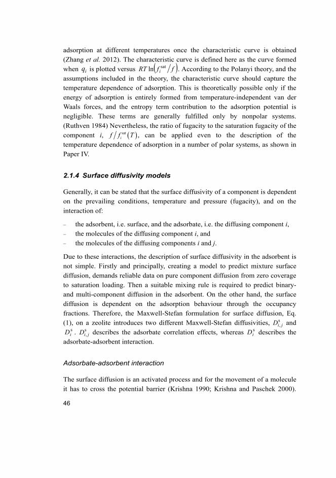
2.1.4 Surface diffusivity models
Generally, it can be stated that the surface diffusivity of a component is dependent
on the prevailing conditions, temperature and pressure (fugacity), and on the
interaction of:
– the adsorbent, i.e. surface, and the adsorbate, i.e. the diffusing component i,
– the molecules of the diffusing component i, and
– the molecules of the diffusing components i and j.
Due to these interactions, the description of surface diffusivity in the adsorbent is
not simple. Firstly and principally, creating a model to predict mixture surface
diffusion, demands reliable data on pure component diffusion from zero coverage
to saturation loading. Then a suitable mixing rule is required to predict binary-
and multi-component diffusion in the adsorbent. On the other hand, the surface
diffusion is dependent on the adsorption behaviour through the occupancy
fractions. Therefore, the Maxwell-Stefan formulation for surface diffusion, Eq.
(1), on a zeolite introduces two different Maxwell-Stefan diffusivities, s, jiD and
siD . s
, jiD describes the adsorbate correlation effects, whereas siD describes the
adsorbate-adsorbent interaction.
Adsorbate-adsorbent interaction
The surface diffusion is an activated process and for the movement of a molecule
it has to cross the potential barrier (Krishna 1990; Krishna and Paschek 2000).

47
Thus, the temperature dependence of siD can be represented with the Arrhenius
dependence:
RTEDTD iaii ,s,0
s exp , (24)
where iaE , is the activation energy of component i. The dependence of surface
diffusion on bulk phase fugacities is indirectly induced through the occupancy
fractions and the adsorption equilibrium. Mechanistically, the Maxwell-Stefan
diffusivity siD can be related to the displacement of the adsorbed molecular
species, , and the jump frequency, , which can be seen to be dependent on the
coverage of the diffusing components (Krishna and Paschek 2000; Reed and
Ehrlich 1981):
s 21iD
z , (25)
where z is the number of neighbour sites. It is expected that the jump frequency
will decrease as a function of occupancy. In addition, if it is assumed that one
molecule can move from one site to another only if the site is free, the probability
of a molecule moving is a function of the number of unoccupied sites. Therefore,
Maxwell-Stefan diffusivity siD can be presented as (Krishna and Paschek 2000):
s s 0i i VD D , (26)
where 0siD is the Maxwell-Stefan diffusivity in the limit of zero loading and
V is a function of the unoccupied site fraction. Hence, if the diffusivity is
assumed to be independent of the occupancy fraction, 1V and Eq. (26) is
transformed into:
0ssii DD . (27)
Eq. (27) is typical for weakly confined molecules in zeolite hosts (Krishna and
Baur 2003). Skoulidas and Sholl (2002) have observed that Eq. (27) is valid for
He, Ar, and Ne in MFI. The assumption of having siD independent of occupancy,
i.e. the component behaves according to Eq. (27), is frequently employed in the
literature (see e.g. Wirawan et al. 2011; Kapteijn et al. 2000; Zhu et al. 2006;
Krishna and Paschek 2000). Generally, the reason for employing the weak
confinement scenario is the lack of reliable data regarding surface diffusivity
loading dependence. In contrast, for strongly confined molecules, the loading
dependency can be described with (Krishna et al. 2004):

48
iii DD 10ss . (28)
Occupancy dependencies that are even more severe than Eq. (28) have been
observed. According to Krishna and Paschek (2000), the experimental data of n-
heptane in 13X appears to follow:
8ss 10 iii DD . (29)
Reed and Ehrlich (1981) have proposed a more general occupancy dependence
model, describing the diffusion of interacting atoms on a square lattice of binding
sites. In their approach, adsorbed atoms interact with each other through the
nearest adatoms only. Finally, a relation is formed for the loading dependency of
Maxwell-Stefan diffusivity:
zii
zi
ii DD
1
10
1ss , (30)
where exp ,i iE RT 1 2 2 1 ,i i i i i and
1 4 1 1 1i i i i .
It is worth noting that unless the system energy is significantly changed as the
adatom is added to a neighbouring site, iE will become vanishingly small in Eq.
(30). Thus, both i and i are equal to 1. Hence, by substituting i and i in Eq.
(30), the occupancy dependence in Eq. (30) is simplified to the strong
confinement scenario presented in Eq. (28). In addition, the weak confinement
scenario Eq. (27) cannot be obtained with any combination of the parameters.
This is due to the fact that the movement of an adatom is dependent on the
vacancy (Krishna et al. 2004). Krishna and van Baten (2005) performed KMC
(Kinetic Monte Carlo) simulations to model the surface diffusivity loading
dependence in MFI using the Reed-Ehrlich approach. Lee (2007) predicted CO2
and CH4 permeation in silicalite-1 based on the occupancy fraction dependence of
Reed-Ehrlich. Recently, Krishna and van Baten (2011) used molecular dynamics
simulation data to estimate the unknown parameters in the Reed-Ehrlich approach
and thereon predicted both single and binary surface diffusivities for a number of
gaseous components, including CO2 and H2, in different adsorbent structures. Eqs.
(27) and (28) were applied in Paper I.
Recently, van den Bergh et al. (2009) proposed the relevant site model for
describing the occupancy dependence of diffusion in zeolites. In their model, the
sites are divided into sites that are relevant and irrelevant for diffusion. The
distinction of the sites can be performed e.g. based on the categorization of

49
window and cage sites as relevant and irrelevant sites, respectively. The Maxwell-
Stefan diffusivity is represented with the relevant site model with (van den Bergh
et al. 2009):
*
,
,*
10iL
iL
i
ii
si
si
b
bDD
, (31)
where *,iLb represents the relevant site adsorption equilibrium constant for the
single-site Langmuir isotherm, and *i is the relevant site occupancy fraction. As
can be seen in Eq. (31), when the relevant site occupancy fraction equals the total
occupancy fraction, the strong confinement scenario is discovered. The
occupancy dependence of siD with different scenarios is illustrated in Fig. 3.
Fig. 3. Maxwell-Stefan surface diffusivity of CO2, sCO2
D , as a function of occupancy
fraction. 2
s 9 2 1CO 0 4.9904 10 m sD . The zero-loading surface diffusivity value is
taken from Paper I.
Fig. 3 shows that the surface diffusivities are, naturally, the same at zero coverage.
On the other hand the strong confinement scenario and the Reed-Ehrlich scenario
coincide as the occupancy fraction reaches 1. In contrast, the weak confinement
scenario is constant throughout the occupancy fraction space. This is not a
feasible scenario that is usable in a general case, as the movement of a molecule
from one site to another is dependent on the number of vacant neighbouring sites.
Thus, the application of the weak confinement scenario, e.g. to the rigorous
description of CO2 surface diffusivity on a wide occupancy fraction domain, is
0 0.1 0.2 0.3 0.4 0.5 0.6 0.7 0.8 0.9 10
0.5
1
1.5
2
2.5
3
3.5
4
4.5
5
x 10-9
DC
O2
s [
m2 s
-1]
Reed-Ehrlich (Paper I)
Weak confinement
Strong confinement

50
not appropriate, as was concluded in Paper I. The extent of the effect of the
different scenarios on the permeation of CO2 on an MFI-type high-silica zeolite
supported membrane can be seen in Fig. 4.
a) b) Fig. 4. a) Permeation flux of CO2 as a function of feed pressure with different surface
diffusivity scenarios and b) the relative difference between the Reed-Ehrlich model
and the weak and strong confinement scenarios. Pressure difference across the
membrane is 0.999 bar. C22 oT . The membrane model used is presented in
Paper I.
As can be seen in Fig. 4a, the scenario selected for surface diffusivity has a clear
influence on the predicted permeation flux of CO2. The relative difference
between the scenarios increases as the occupancy fraction increases, as shown in
Fig. 4b. It is also worth noting that the permeation flux profiles approach each
other at low pressure as is to be expected due to the same 0sCO2
D value of the
scenarios.
As a whole, it can be stated that there are multiple scenarios that the surface
diffusivity of a component may follow. The determination of the appropriate
scenario for each case is dependent both on the degree of confinement within the
adsorbent, and on the characteristics of the adsorbate i - adsorbate i interactions
(Krishna and Baur 2003; Skoulidas et al. 2003).
Adsorbate-adsorbate interaction
The binary exchange coefficients s, jiD , or adsorbate interaction diffusivities, can
be interpreted as the capability of an adsorbate j to replace an adsorbate i on a
sorption site. Generally, the consequence of this interaction is that the faster
diffusing adsorbate is slowed down by the slower moving adsorbate as
0 5 10 15 20 25 30 35 40-20
-10
0
10
20
30
40
Pfeed [bar]
Rel
ativ
e di
ffer
ence
[%
]
Weak confinement
Strong confinement
0 5 10 15 20 25 30 35 40
0.2
0.4
0.6
0.8
1
1.2
Pfeed [bar]
NC
O2 [
mol
s-1
m-2
]
Reed-Ehrlich (Paper I)
Weak confinementStrong confinement

51
demonstrated in Paper I. Even mutual slowing down effects have been observed
with water-methanol and water-ethanol mixtures (Krishna and van Baten 2010c).
However, the literature models assume that the mutual slowing effects can be
neglected, which has been shown to apply e.g. in gas mixtures.
Krishna and van Baten (2011) noticed that based on molecular dynamics
simulations, regardless of the topology of the studied adsorbent, the correlation
effects increase with increasing pore concentrations, i.e. the magnitude of s, jiD is
reduced significantly. In addition, the movement of the slower moving adsorbate
is accelerated. In the case of a single adsorbed component diffusing, siD is
equivalent to the ‘corrected’ diffusivity s, jiD (Skoulidas et al. 2003). This can also
be deduced from the Maxwell-Stefan formulation, Eq. (1), for single-component
permeation.
Because there are no fundamental models as yet to predict the binary
exchange coefficients, s, jiD is generally estimated with different models (Krishna
and Paschek 2000). The literature attempts to describe binary exchange
coefficients can be summarized to include the following dependence:
ji
j
ji
ijjiiji
sji DDqqTD
,,,,,, s,
s,
satsat, . (32)
As can be seen in Eq. (32), the binary exchange coefficients are dependent on the
saturation loadings, the self-exchange coefficients of the pure species, i.e. s,iiD
and s, jjD , and their compositions in the adsorbed mixture at a given temperature.
Note that the Onsager reciprocal relations demand that s,
s, ijji DD (Krishna and
Paschek 2002). In practice a relationship that strictly follows Eq. (32) is difficult
to apply, due to the self-exchange coefficient dependence of the relation.
Self-exchange coefficients
Self-exchange coefficients can be determined based on siD and self,iD , providing
that they are known independently (Skoulidas et al. 2003). Krishna and Paschek
(2002) derived a relation between siD and self,iD for a binary mixture with tagged
and untagged species, both having identical siD :
s,
s
self, 11
ii
i
i
i
DD
D
. (33)

52
Next, based on the data on the self-diffusivity self,iD and surface diffusivity siD of
the species the self-exchange coefficients s,i iD can be calculated. Skoulidas et al.
(2003) noticed that the dependence follows the empirical expression:
iiiiii DD expss, , (34)
where i and i are fitted parameters dependent on both the component i and the
topology of the particular adsorbent. The ratio s s,i i iD D can be seen as a measure
of the degree of correlation for the unary diffusion of component i. s s,i i iD D
increases as the pore concentration increases, i.e. the movement of individual
molecules become increasingly correlated. (Krishna and van Baten 2011) Later on,
e.g. Krishna and van Baten (2005) and Lee (2007) applied Eq. (34) in the
description of permeation in zeolites. Recently, based on MD-simulated data,
Krishna and van Baten (2011) fitted the degree of correlation for unary diffusion
with the expression
2s
s
iiiiii,i
i cbaD
D , (35)
where ia , ib and ic are fitted constants dependent on the studied component i
and the adsorbent properties. The degree of correlation can be viewed in detail in
Fig. 5.

53
Fig. 5. s s,i i iD D of CO2 in MFI at the temperature of 300 K as a function of
occupancy fraction. 2
sat 1CO 5.1876 mol kgq . The literature models are based on MD
simulation studies.
As shown in Fig. 5, s s,i i iD D decreases as the occupancy fraction of CO2
increases. The decrease means in turn that the degree of correlation increases as
the pore concentration increases, as expected. The practical consequence of the
decrease in the ratio is that the predicted binary exchange coefficients have
smaller values and the movement of the components is slowed down even from
the values calculated based on s .iD In addition, Fig. 5 shows that the ratio
approaches the value of 1 as the occupancy fraction approaches zero. On the other
hand, it is common that the ratio cannot be determined due to the insufficiency of
available data on the system. Therefore, the approximation ss, iii DD is
frequently applied.
Binary exchange coefficients
Binary correlation effects can be predicted with relationships originally developed
for the description of diffusion in bulk liquid mixtures by Vignes (1966):
ij xij
xjiji DDD ,,, , (36)
0 0.1 0.2 0.3 0.4 0.5 0.6 0.7 0.8 0.9 10.1
0.2
0.3
0.4
0.5
0.6
0.7
0.8
Ds i,i
( )
/ D
s i( )
Lee (2007)
Krishna and van Baten (2011)
Krishna and van Baten (2005)

54
where jiD , and
ijD , are the infinite dilution diffusion coefficient of i and j,
respectively. Similarly, inspired by the bulk liquid diffusivity descriptions, linear
and square root interpolation formulas for surface diffusion binary exchange
coefficients have also been suggested (Krishna and Paschek 2002). However, the
linear and square root interpolation formulas have not been applied widely in
conjunction with surface diffusion.
In the Vignes relationship, Eq. (36), the binary exchange diffusivities are
exponentially related to the mole fraction of each component. However, the mole
fraction is not very suitable as a measure of the adsorbed species proportion on an
adsorbent. Thus, Krishna (1990) generalized the Vignes relationship to the
diffusion of adsorbed species with the usage of occupancy fractions instead of
mole fractions:
jijjii
jiji DDD
sss, . (37)
On the other hand, if the saturation loading of each component is equal or mole
fractions are usable, Eq. (37) transforms into (Skoulidas et al. 2003):
jijjii qqqj
qqqiji DDD
sss
, . (38)
Assuming that we have obtained the self-exchange diffusivities s,iiD
independently from Maxwell-Stefan diffusivities siD , a relationship based on Eq.
(32) can be formulated as proposed by Skoulidas et al. (2003):
jijjii qqqjji
qqqiijjij DqDqDq
s
,sats
,sats
,sat . (39)
Skoulidas et al. (2003) successfully applied the interpolation formula, Eq. (39), to
predict the diffusivities of a mixture of CH4/CF4. Recently, van den Bergh et al.
(2010) applied Eq. (39) in conjunction with the relevant site model to model the
diffusion of light gases in zeolites. It is worth noting that Eq. (39) returns to the
form of Eq. (38) if the saturation loadings of the perspective components are
equal and ss, iii DD . The main drawback of Eq. (39) in general is that the
saturation loadings are required. In Paper I, a Vignes-type interpolation formula
including the self-exchange correlations:
jijjii
jjiiji DDD
s,
s,
s, (40)
was used due to the availability of data on the degree of correlation for unary
diffusion from Krishna and van Baten (2011). Krishna and van Baten (2009, 2011)

55
also proposed that the mole fractions could be used instead of occupancy fractions
in Eq. (40). The differences between the predictions of the proposed binary
exchange correlation formulas can be observed in Fig. 6.
Fig. 6. Binary exchange surface diffusivities with different literature formulas for
diffusion of equimolar bulk phase mixtures of H2 and CO2 at 23°C as a function of the
bulk gas phase pressure. The adsorption and diffusivity parameters used are from
Paper I.
As can be seen in Fig. 6, the selection of the binary exchange formula is relevant,
especially at high pressure. However, all the formulas predict surface diffusivities
with the same order of magnitude. The reason for this is the strong effect of CO2
on the binary exchange diffusivity. The proportion of CO2 adsorbed is clearly
higher than the proportion of H2. Thus, sCO
sH,CO 222
DD or sCO,CO
sH,CO 2222
DD depending on the formula in question. Essentially, self-exchange diffusivities
decline as pressure increases, but the adsorption equilibrium shifts at the same
time slightly towards preferring hydrogen adsorption in comparison with carbon
dioxide. This interplay between the effects means that in Fig. 6 the trends between
the formulas differ, i.e. also qualitatively. As a whole, the usage of self-exchange
diffusivities is a more theoretically sound approach. Nevertheless, the selection
between the formulas using self-exchange diffusivities is not self-evident, and
demands further investigation in the future.
5 10 15 20 25 30 35 402.5
3
3.5
4
4.5
5
x 10-9
P [bar]
Ds C
O2,
H2 [
m2 s
-1]
Krishna and van Baten (2009)
Paper I
Krishna (1990)Vignes
Skoulidas et al. (2003)

56
Although the above mentioned models for predicting the binary exchange
diffusivities of the adsorbate have been shown to apply to the description of a
multitude of mixtures, there is still work to be done in different applications. One
important application, where the models fail, is the surface diffusion of water-
alcohol mixtures as shown by Krishna and van Baten (2010a, 2010b, 2010c). The
failure is due to the hydrogen bonding between water-alcohol molecules.
2.2 Liquid-liquid phase separation
Modelling liquid-liquid phase separation can be performed starting from the
description of the liquid-liquid equilibrium. The phase equilibrium can be
described with the thermodynamic potentials. A general liquid-liquid equilibrium
problem consists of finding the correct number and types of phases and their
corresponding equilibrium compositions such that the Gibbs free energy of the
system is at the minimum. A considerable number of methods and algorithms
have been formulated to solve the phase equilibrium problem. Generally, the basis
of the algorithms is to solve a sequence of sub-problems. The algorithms can be
separated into two groups: equation-solving and Gibbs free energy minimization
approaches (Wakeham and Stateva 2004; Rangaiah 2001).
2.2.1 Equation-solving approach
The equation-solving approaches solve a set of nonlinear equations, based on the
component mass balances and phase equilibrium relations. In practice, the
equation set formed in the equation-solving approach describes the liquid-liquid
phase separation equipment operating isothermally or/and it is assumed that the
energy changes attributed to the phase changes are negligible.
Let us first assume a mixture of n components with molar amounts
(N1,N2,...,Nn). In addition, let us assume that the mixture may split into F liquid
phases. Then the following group of equations can be solved to obtain the
equilibrium compositions and relative amounts of the phases at temperature T and
pressure P:
F
jijij Nx
1, , i = 1,2,..., n, (41)
LFi
Li
Li Fiii
xxx,2,1, ,2,1, ... , i = 1,2,...,n, (42)

57
n
ijix
1, 1, j = 1,2,..., F, (43)
where j is the total amount of phase j. It is worth noting that the activity
coefficients are temperature-dependent. Thus, Eqs. (41)-(43) have to be solved
again or an energy balance for the system has to be introduced, if the energy
changes related to the phase appearance or disappearance are significant and the
temperature of the system changes significantly. On the other hand, Eqs. (41)-(43)
fulfil only the necessary conditions of equality of the chemical potential of every
component in each phase. Hence, Eqs. (41)-(43) are always fulfilled when the
composition of each phase is the same, i.e. even when the actual phase
configuration and compositions are different. However, they do not ensure that
the sufficient condition of phase equilibrium is satisfied (Baker et al. 1982; Cairns
and Furzer 1990; Rangaiah 2001; Michelsen and Mollerup 2007). The sufficient
condition refers here to the fact that the phase configuration of the system is
fulfilled only when the Gibbs energy of the resulting system is at minimum.
In practice, the insufficiency of the approach may signify that the solved
compositions and relative amounts do not correspond to the actual phase
configuration. In addition, the straightforward application of the equation set in
Eqs. (41)-(43) demands knowledge of the possible number of phases. Therefore,
the approach is generally used only in conjunction with short-cut calculation
routines and when a considerable amount of problem-dependent data is available.
2.2.2 Minimization of Gibbs energy
The second approach of minimizing the Gibbs energy yields both the necessary
and sufficient conditions of phase equilibrium (Tolsma and Barton 2000a). Thus,
the Gibbs free energy minimization approach is more preferable than the
equation-solving approach in the robust evaluation of phase equilibrium
conditions. The core of the Gibbs energy minimization approaches is to evaluate
the multicomponent and multiphase equilibrium based on the global minimum of
the Gibbs free energy of the system (Baker et al. 1982). Fundamentally, there are
two routes that can be followed to obtain or verify that an equilibrium solution
corresponds to the global minimum of the Gibbs free energy. The two
optimization problems associated with these approaches are the direct
minimization of the Gibbs free energy and the minimization of the tangent plane
distance function (TPDF). In this thesis, the minimization of TPDF is considered.
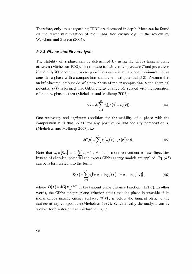
58
Therefore, only issues regarding TPDF are discussed in depth. More can be found
on the direct minimization of the Gibbs free energy e.g. in the review by
Wakeham and Stateva (2004).
2.2.3 Phase stability analysis
The stability of a phase can be determined by using the Gibbs tangent plane
criterion (Michelsen 1982). The mixture is stable at temperature T and pressure P
if and only if the total Gibbs energy of the system is at its global minimum. Let us
consider a phase with a composition z and chemical potential ( ) z . Assume that
an infinitesimal amount e of a new phase of molar composition x and chemical
potential ( ) z is formed. The Gibbs energy change G related with the formation
of the new phase is then (Michelsen and Mollerup 2007):
n
iiiixeG
1
zx . (44)
One necessary and sufficient condition for the stability of a phase with the
composition z is that 0G for any positive e and for any composition x
(Michelsen and Mollerup 2007), i.e.
01
n
iiiixG zxx . (45)
Note that 1,0ix and 1ix . As it is more convenient to use fugacities
instead of chemical potential and excess Gibbs energy models are applied, Eq. (45)
can be reformulated into the form:
n
i
Lii
Liii zxxD
1
lnlnlnln zxx , (46)
where D G RTx x is the tangent plane distance function (TPDF). In other
words, the Gibbs tangent plane criterion states that the phase is unstable if its
molar Gibbs mixing energy surface, m x , is below the tangent plane to the
surface at any composition (Michelsen 1982). Schematically the analysis can be
viewed for a water-aniline mixture in Fig. 7.

59
a)
b) Fig. 7. Gibbs mixing surface and tangent plane to the surface of a water (1) – aniline
(2) mixture at a) 3.07.0z and b) 8.02.0z .
As shown in Fig. 7, the Gibbs mixing surface falls below the tangent plane in Fig.
7a. Instead, in Fig. 7b the tangent plane is below the Gibbs mixing surface at all
compositions. Thus, according to the tangent plane distance criterion, the mixture
is unstable in Fig. 7a and stable in Fig. 7b at the given T and P. Numerically, the
0 0.1 0.2 0.3 0.4 0.5 0.6 0.7 0.8 0.9 1-0.2
-0.15
-0.1
-0.05
0
0.05
0.1
0.15
xw ater
m( x
)
D(x)<0
z
0 0.1 0.2 0.3 0.4 0.5 0.6 0.7 0.8 0.9 1-0.15
-0.1
-0.05
0
0.05
0.1
xw ater
m( x
)
z
D(x)>0
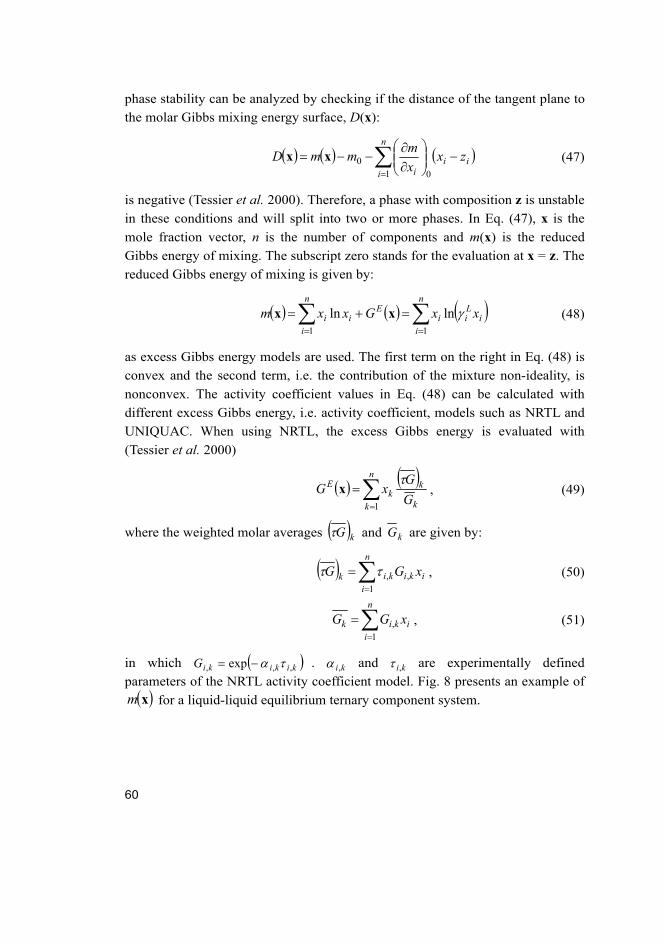
60
phase stability can be analyzed by checking if the distance of the tangent plane to
the molar Gibbs mixing energy surface, D(x):
n
iii
i
zxx
mmmD
1 00xx (47)
is negative (Tessier et al. 2000). Therefore, a phase with composition z is unstable
in these conditions and will split into two or more phases. In Eq. (47), x is the
mole fraction vector, n is the number of components and m(x) is the reduced
Gibbs energy of mixing. The subscript zero stands for the evaluation at x = z. The
reduced Gibbs energy of mixing is given by:
n
ii
Lii
n
i
Eii xxGxxm
11
lnln xx (48)
as excess Gibbs energy models are used. The first term on the right in Eq. (48) is
convex and the second term, i.e. the contribution of the mixture non-ideality, is
nonconvex. The activity coefficient values in Eq. (48) can be calculated with
different excess Gibbs energy, i.e. activity coefficient, models such as NRTL and
UNIQUAC. When using NRTL, the excess Gibbs energy is evaluated with
(Tessier et al. 2000)
n
k k
kk
E
G
GxG
1
x , (49)
where the weighted molar averages kG and kG are given by:
n
iikikik xGG
1,, , (50)
n
iikik xGG
1, , (51)
in which kikikiG ,,, exp . ki, and ki, are experimentally defined
parameters of the NRTL activity coefficient model. Fig. 8 presents an example of xm for a liquid-liquid equilibrium ternary component system.

61
Fig. 8. Reduced Gibbs energy of mixing for Case 3 in Paper V.
toluenewateraniline 1 xxx .
The main difficulties in the minimization of D(x) arise in general from the non-
convex term in Eq. (48). The Gibbs tangent plane criterion is generally checked
by minimizing D(x) with a mole fraction restriction. This minimization problem
can either be solved directly or by solving an equivalent set of nonlinear
equations for the stationary points of D(x) (Tessier et al. 2000). An example of the
D(x) surface can be seen in Fig. 9.
xtoluene
x wat
er
-0.4
-0.3
-0.2
-0.1
0
0.1
0.2
0.3
-0.3
-0.2-0.1
00.10.2
0 0.1 0.2 0.3 0.4 0.5 0.6 0.7 0.8 0.9 10
0.1
0.2
0.3
0.4
0.5
0.6
0.7
0.8
0.9
1

62
Fig. 9. The tangent plane distance contour plot for Case 3 in Paper V. The mixture
studied is 50005.0,20006.0,29989.0z and marked with ‘’.
In Fig. 9 with certain test compositions, D(x) is negative, indicating that the
mixture at composition z is unstable and will split into two or more phases
depending on the subsequent flash calculations. Hence, in many cases the
knowledge of phase splitting can be obtained efficiently with local solving
methods. However, in order to obtain feasible estimates for the individual phase
compositions for the subsequent flash calculations, at least the global minimum of
D should be sought, which cannot be ascertained with local solving methods.
The global minimum of TPDF and all the other roots of the problem can be
solved by directly minimizing the TPDF or creating a set of nonlinear equations
for the stationary points of D(x). Schematically, the solution of the stationary
points can be seen in Fig. 10.
0 0.1 0.2 0.3 0.4 0.5 0.6 0.7 0.8 0.9 10
0.1
0.2
0.3
0.4
0.5
0.6
0.7
0.8
0.9
1
xtoluene
x wat
er
0
0
0.10.20.3
0.4
-0.1
-0.2
0.1 0.2 0.3 0.4

63
a)
b)
Fig. 10. a) Tangent plane distance function and b) Gibbs mixing surface of a water-
aniline mixture 3.07.0z including stationary points and respective tangent
planes.
A number of issues can be seen in Fig. 10. The binary mixture of water and
aniline is unstable at the studied composition because the tangent plane distance
function value is negative at two stationary points in Fig. 10a. Note that only one
stationary point with a negative D(x) is required to verify instability. Secondly,
the studied mixture is a local maximum on the D(x) curve as can be seen in Fig.
0 0.1 0.2 0.3 0.4 0.5 0.6 0.7 0.8 0.9 1
-0.1
-0.05
0
0.05
0.1
0.15
D( x
)
xw ater
0 0.1 0.2 0.3 0.4 0.5 0.6 0.7 0.8 0.9 1-0.2
-0.1
0
0.1
xw ater
m( x
)
Studied mixture
Stationary pointsTangent plane

64
10a. Therefore, the instability of the studied mixture can be determined with the
evaluation of D(x) at a composition infinitesimally close to the composition.
However, this evaluation will not supply a good initial guess for the subsequent
phase equilibrium calculations. Instead, the stationary points with a negative D(x)
value can be used to initiate the phase equilibrium calculations efficiently.
To obtain the locations of all the stationary points, the following equation set
is solved (Tessier et al. 2000):
00
nini x
m
x
m
x
m
x
m, i = 1,..., n − 1; (52)
n
iix
1
01 . (53)
It is also noteworthy that at all the stationary points the tangent planes evaluated
on the basis of m x are parallel in Fig. 10b as expected, when applying Eqs.
(52)-(53) for a binary mixture. The set of equations, Eqs. (52)-(53), can be
reformulated by using Eq. (48) into
0lnln
zx ii
n
i
n
i ssz
z
x
x, i = 1,..., n − 1; (54)
n
iix
1
01 , (55)
where xis is represented by:
n
k k
knkik
k
knknkikik
n
n
i
ii
G
GGG
G
GGx
G
G
G
Gxs
12
,,,,,, , (56)
if NRTL is used to describe the liquid phase activity coefficients. The equation set,
Eqs. (54) and (55), has a trivial root, which corresponds to the composition of the
inspected mixture (x = z). The equation set may also have multiple non-trivial
feasible roots, i.e. mixture compositions that fulfil Eqs. (54) and (55) and the
condition, 1,0ix , as was shown in Fig. 10. Thus, the problem can be termed a
multiplicity problem. The number of roots depends on the case studied, i.e. the
components, conditions, and the location of the mixture composition with respect
to phase splitting, and the thermodynamic model used to describe the phase
equilibrium.
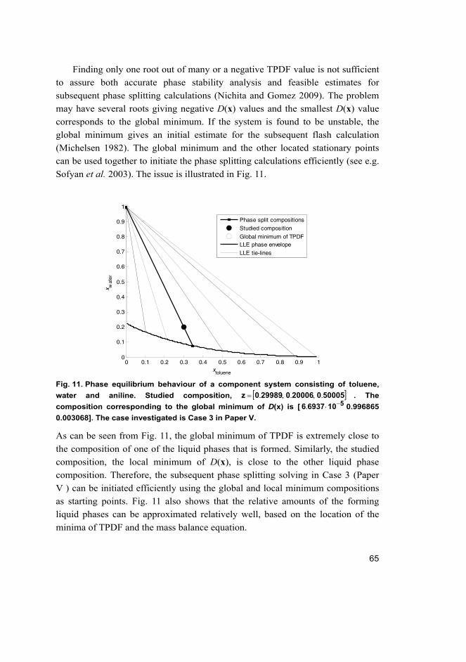
65
Finding only one root out of many or a negative TPDF value is not sufficient
to assure both accurate phase stability analysis and feasible estimates for
subsequent phase splitting calculations (Nichita and Gomez 2009). The problem
may have several roots giving negative D(x) values and the smallest D(x) value
corresponds to the global minimum. If the system is found to be unstable, the
global minimum gives an initial estimate for the subsequent flash calculation
(Michelsen 1982). The global minimum and the other located stationary points
can be used together to initiate the phase splitting calculations efficiently (see e.g.
Sofyan et al. 2003). The issue is illustrated in Fig. 11.
Fig. 11. Phase equilibrium behaviour of a component system consisting of toluene,
water and aniline. Studied composition, 500050200060299890z .,.,. . The
composition corresponding to the global minimum of D(x) is [ 51069376 . 0.996865
0.003068]. The case investigated is Case 3 in Paper V.
As can be seen from Fig. 11, the global minimum of TPDF is extremely close to
the composition of one of the liquid phases that is formed. Similarly, the studied
composition, the local minimum of D(x), is close to the other liquid phase
composition. Therefore, the subsequent phase splitting solving in Case 3 (Paper
V ) can be initiated efficiently using the global and local minimum compositions
as starting points. Fig. 11 also shows that the relative amounts of the forming
liquid phases can be approximated relatively well, based on the location of the
minima of TPDF and the mass balance equation.
0 0.1 0.2 0.3 0.4 0.5 0.6 0.7 0.8 0.9 10
0.1
0.2
0.3
0.4
0.5
0.6
0.7
0.8
0.9
1
xtoluene
x wat
er
Phase split compositions
Studied composition
Global minimum of TPDFLLE phase envelope
LLE tie-lines

66
Verification of finding a consistent number of feasible solutions
The correct number and type of solutions of TPDF are not known beforehand.
Thus, it is evident that the knowledge that all the feasible solutions of the problem
have been found is in practice vital to ascertain the robustness of the problem
solving. Currently, there is no tool available that can either verify that all the
solutions have been found or evaluate the relative number of solutions before
solving the problem. However, Wasylkiewicz et al. (1996) have presented the
topological criterion, which can be used to verify the consistency of the stationary
points found with respect to the TPDF surface topology. The criterion was applied
in Papers III and V to verify that the number of feasible solutions found is
consistent. The criterion states that, for an n component mixture:
dd NNNN 11 oddsad
evensadminmax , (57)
where 1 nd , maxN is the number of maxima of xD , minN is the number of
minima, evensadN is the number of saddles with an even number of negative
eigenvalues, and oddsadN is the number of saddles with an odd number of negative
eigenvalues of the Hessian matrix xH ˆD , where x̂ is a mole fraction vector
with 1n elements of vector x . The type of stationary point x̂ can be
determined from the eigenvalues, ie , 1,...,1 ni , of the Hessian matrix xH ˆD
as follows:
– If all the eigenvalues are positive, the stationary point is a minimum.
– If all the eigenvalues are negative, the stationary point is a maximum.
– If 2d and there is at least one negative eigenvalue and at least one positive
eigenvalue, the stationary point is a saddle.

67
3 Separation process model solution methods
Separation process model formulation is dependent on multiple issues. From the
perspective of solving the model, the existence of possible temporal- and
location- dependent gradients, i.e. tc or rc , inside the process equipment
dictates to a great extent the selection of the solution strategy. Table 5 shows a
selection of solution strategies used in process model solution.
Table 5. Selected mathematical solution strategies for different process models.
Model Mathematical type of
model
Solution strategies Reference
Gas-liquid reactor models
DADM with FPM1
t
c
,
2
2l
c,
l
c
,r
c
, c †
t
c
,
2
2r
c, c
PDE + PDE
discretize r and l and
integrate t
Romanainen
(1994)
SADM with FM1 2
2l
c,
l
c
,r
c
, c PDE + BVP
discretize r/l and solve
l/r
discretize r and l and
solve NLE
Romanainen
(1994)
STS with FM1
r
c
,
2
2r
cc , c
ODE + BVP
discretize r and solve
NLE
include STS to FM and
solve BVP
Romanainen
(1994)
Automotive catalytic converter
t
y
,
2
2l
y,
l
y
, y
t
gT
,
2
2l
gT
,l
gT
, gT †
t
sT,
2
2l
sT, sT †
PDE
discretize l and
integrate t
Kangas et al.
(2002)

68
Model Mathematical type of
model
Solution strategies Reference
Membrane separation
with support, finite Di,j
z
θ
, θ ODE
discretize z and solve
NLE
Paper I
no support, pure
component permeation z
θ
, θ ODE
integrate z
Sandström et al.
(2011)
no support, infinite Di,j
z
θ
, θ Analytic solution Krishna and Baur
(2004)
Decanter ( ) f x 0 NLE
solve NLE
Paper V
Mixture adsorption equilibrium Papers I and II
Thermally-coupled distillation
columns
Malinen and
Tanskanen
(2009) 1Dynamic bubble column with axial dispersion (DADM), Film model (FM), Film-penetration model (FPM),
Steady state bubble column with axial dispersion model (SADM), Steady state tanks-in-series model
(STS). † c is the vector of component concentrations, s
T is the vector of the solid temperature, g
T is the
vector of gas phase temperatures, r and l are the radial and length coordinates, respectively.
As can be seen in Table 5, it is common to convert a process model composed of
an ODE set into the form of an NLE set by first discretizing along the physical
coordinates and then solving the resulting NLE set. This is especially true when
the steady-state behaviour of a process is being studied. However, even after the
conversion of the problem to an NLE set, the solving of the problem is not certain.
The solving of an NLE set is difficult for various reasons:
– Some of the functions can be undefined for certain variable values, which
creates a discontinuity (see e.g. Shacham and Brauner (2002)) or a boundary
across the solution path.
– The equation set may have solutions that are not physically feasible.
– The functions may be highly nonlinear and/or badly scaled.
– The feasible selection of the starting (or initial) point may be difficult.
In addition, in separation process models, like the heterogeneous distillation
column and membrane separation models, the number of equations and variables
in the formed NLE set may be high and the Jacobian of the equation set may be
sparse, i.e. the Jacobian matrix has a large portion of elements having a value of
zero. This is illustrated in Fig. 12.

69
Fig. 12. Numerical sparsity pattern of the Jacobian of the membrane separation model
used in Paper I. The number of axial elements along the zeolite film is 20. The sparsity
pattern of the Jacobian was evaluated using MATLAB. The number of non-zero
elements () is 1560.
A sparse Jacobian in turn may cause the solving of the NLE set to be inefficient
unless the Jacobian matrix can be determined analytically or the Jacobian matrix
structure is taken into account in the numerical Jacobian matrix approximation.
NLE sets are frequently solved iteratively with Newton-Raphson based
solution methods. The Newton and quasi-Newton methods are widely used local
methods because they are simple and, theoretically at least, superlinearly
convergent. These methods will not converge generally unless an initial guess is
supplied that is reasonably close to the solution. In addition, these methods
typically achieve only one solution from one initial point.
3.1 Solution of the membrane separation model
In the case of a membrane separation process model as described in Paper I, it is
important to note that the model has only one solution and a reasonably good
initial guess can be supplied by using application-dependent knowledge and a
simplified membrane model. Thus, a successful solution with Newton-based
solving methods can be ascertained. However, the solution may still travel outside
0 50 100 150 200
0
20
40
60
80
100
120
140
160
180
200
nz = 1560
70
the feasible problem domain without using variables mapping, for instance.
Therefore, the variables mapping was applied in the solution of the membrane
and mixture adsorption equilibrium models in Paper I.
The application of a Newton-based local solving method demands first that
the Maxwell-Stefan equations representing the membrane separation through the
zeolite pores, Eq. (4), are modified into a form compatible with NLE equations,
as shown in Table 5, i.e. in the form 0xf . This can be performed with the
discretization of the zeolite film into elements as applied in Paper I. The film was
discretized into 21 spatially uniform grid points, i.e. equalling 20 elements. In the
literature, 50 or even more elements have been used (Wirawan et al. 2011; Graaf
1999), but the selected number of elements was adequate for this application as
the occupancy fraction profiles were relatively linear across the zeolite film. One
reason for the relatively linear gradients is that the surface diffusivities have only
mild occupancy dependences in the domain investigated. Otherwise, the
implementation of Eq. (29), for instance, in a membrane separation model would
have a clear effect on the gradients. This is due to the severity of the occupancy
dependence in Eq. (29). Similarly, the occupancy dependence has an effect on the
selection of a method to evaluate the elements of zθ .
In this context it is worth noting that the selection of a method to evaluate
numerically the elements of zθ has an effect on the robustness of the solving
strategy. In Paper I, the terms of zθ in Eq. (4) were then approximated with
classical three-point, second-order finite differences. In addition, the selection of
a numerical method to approximate the gradients is not straightforward. The finite
differences can easily be formulated although the number of grid points should be
large. On the other hand, when the problem has steep gradients, the finite
difference or the finite element method could be preferred. However, if the
problem is relatively easy to solve and the problem solution is smooth, a weighted
residuals method should be preferred. (Finlayson 1980) It is difficult to determine
the steepness of the gradients in the membrane model beforehand. Hence, the
finite difference method was selected in this work.
After discretization and implementation in the Matlab environment, the fsolve
function of Matlab can be applied in the model solution. In addition to the upper
level solving of the equation set, an iterative solution of the adsorption
equilibrium is required as the relation of occupancy fractions and partial
pressures/fugacities is calculated in the thermodynamic factor matrix, as
presented in Eq. (3). The iterative solution of the thermodynamic factors based on
IAST is the main factor that determines solution time. Note however that the

71
iterative solution of the thermodynamic factor matrix is demanded when studying
mixture separation, not when investigating pure component permeation. Hence, in
Paper I, the following solution strategy was applied as depicted in Fig. 13.

72
Fig. 13. Solution strategy of the membrane separation model built in Paper I.

73
As can be seen in Fig. 13, the solution of the membrane model demanded a
relatively large amount of problem-dependent knowledge. In addition, the
solution time was extensive due to the iterative solution of the sub-problem, i.e.
the evaluation of the thermodynamic factor matrix elements. However, the
solution strategy guaranteed that the model was solved robustly.
3.2 Solution of a phase stability analysis problem
In contrast, the solution of a phase stability analysis problem, as formulated in
Section 2.2.3, requires advanced solving strategies preferentially in the form of a
robust solving method. However, solving strategies with application-dependent
knowledge utilizing local solution methods have also been proposed in the
literature. The main features of a phase stability analysis problem that cause
difficulties during the solution of the problem are:
– all the feasible solutions of the equation set have to be discovered,
– the equation set is highly nonlinear,
– all the variables have strict physically determined boundaries,
– the equation set includes logarithmic terms,
– the Jacobian of the equation set is full, and
– the trivial solution of the equation set cannot be avoided.
Thus, due to the considerable problems caused by the features, the usage of local
solving methods demands heuristics (see e.g. Michelsen 1982) in terms of
choosing the initial guess, and in practice, multiple initial guesses. However, even
with the use of numerous starting points along with heuristics it cannot be
guaranteed that all the minima of TPDF will be found (Wasylkiewicz et al. 1996).
Therefore, e.g. Michelsen and Mollerup (2007) set a more modest target for the
solution of the problem: ”A less ambitious approach is to perform the search for
local minima with a number of judiciously selected initial estimates in the hope
that these searches will uncover at least all the negative minima.” Thus, the
formulation of a robust solving strategy is vital to enable robust phase stability
analysis. Hence, it is not surprising that the usage of global solution methods in
phase stability analysis has been intensive in the literature during recent two
decades. In order to determine robustly if a phase is stable or not, several
numerical techniques, global solving methods, have been proposed during the
years to solve the problem, as shown in Table 6.
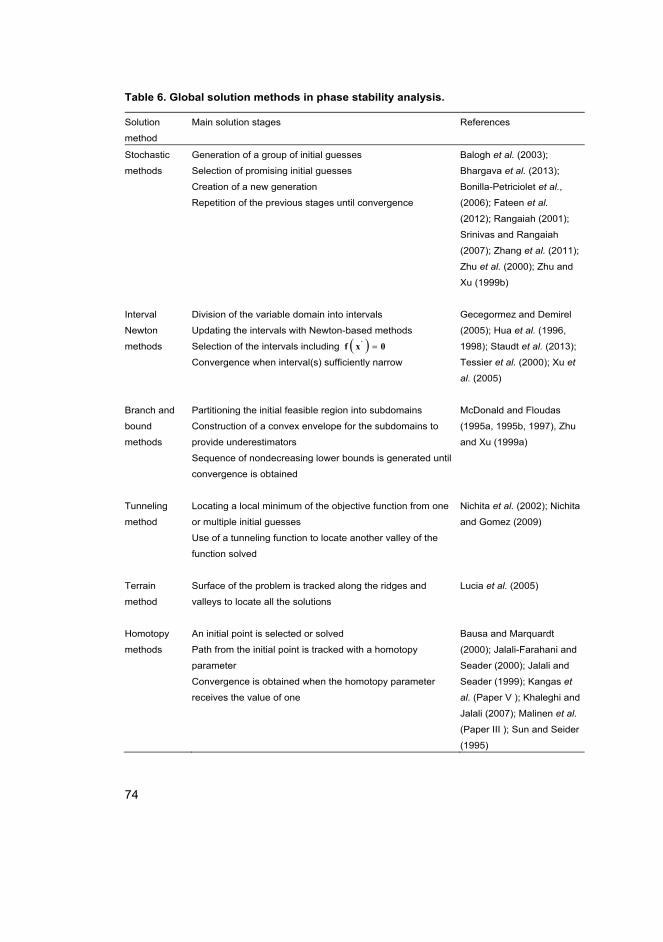
74
Table 6. Global solution methods in phase stability analysis.
Solution
method
Main solution stages References
Stochastic
methods
Generation of a group of initial guesses
Selection of promising initial guesses
Creation of a new generation
Repetition of the previous stages until convergence
Balogh et al. (2003);
Bhargava et al. (2013);
Bonilla-Petriciolet et al.,
(2006); Fateen et al.
(2012); Rangaiah (2001);
Srinivas and Rangaiah
(2007); Zhang et al. (2011);
Zhu et al. (2000); Zhu and
Xu (1999b)
Interval
Newton
methods
Division of the variable domain into intervals
Updating the intervals with Newton-based methods
Selection of the intervals including *
f x 0
Convergence when interval(s) sufficiently narrow
Gecegormez and Demirel
(2005); Hua et al. (1996,
1998); Staudt et al. (2013);
Tessier et al. (2000); Xu et
al. (2005)
Branch and
bound
methods
Partitioning the initial feasible region into subdomains
Construction of a convex envelope for the subdomains to
provide underestimators
Sequence of nondecreasing lower bounds is generated until
convergence is obtained
McDonald and Floudas
(1995a, 1995b, 1997), Zhu
and Xu (1999a)
Tunneling
method
Locating a local minimum of the objective function from one
or multiple initial guesses
Use of a tunneling function to locate another valley of the
function solved
Nichita et al. (2002); Nichita
and Gomez (2009)
Terrain
method
Surface of the problem is tracked along the ridges and
valleys to locate all the solutions
Lucia et al. (2005)
Homotopy
methods
An initial point is selected or solved
Path from the initial point is tracked with a homotopy
parameter
Convergence is obtained when the homotopy parameter
receives the value of one
Bausa and Marquardt
(2000); Jalali-Farahani and
Seader (2000); Jalali and
Seader (1999); Kangas et
al. (Paper V ); Khaleghi and
Jalali (2007); Malinen et al.
(Paper III ); Sun and Seider
(1995)

75
As Table 6 shows, the majority of the literature studies use stochastic methods.
However, the application of stochastic methods in chemical process simulation
software has not progressed significantly. The main reasons for the slow progress
in the application of stochastic methods, and in fact of all the global solving
methods, are the failures of finding all the roots of TPDF and the considerable
solving time of the methods. The solving time becomes impractical especially
when the number of components (variables) increases in the studied system.
In addition, homotopy methods have attracted considerable interest, as shown
in Table 6. The main issue to be tackled with the homotopy methods is that only
some roots of TPDF are obtained from a single initial guess. Homotopy methods
are also generally used in the field of phase behaviour analysis to solve NLE sets
and the methods have already been applied in commercial chemical simulation
software such as ASPENPlus. The literature regarding homotopy methods in
phase equilibrium studies can be divided into the use of either problem-dependent
or problem-independent homotopies.
3.2.1 Problem-dependent homotopies
The emphasis in the literature is to take application properties into account (see
e.g. Fidkowski et al. (1993), Eckert and Kubicek (1997), Tolsma and Barton
(2000a, 2000b), Wasylkiewicz et al. (1999), Wang et al. (1999) or Aslam and
Sunol (2006)). Thus, the homotopy is reformed frequently into a problem-
dependent form. The problem dependency of a homotopy can be defined to
include one or several of the options below:
– usage of a problem variable in place of an artificial homotopy parameter,
– change in the properties of the problem along the homotopy path, e.g. the
non-ideality of the mixture increases from Raoult’s law behaviour to actual
non-ideal behaviour as the value of the homotopy parameter is increased,
– usage of the homotopy parameter only for certain equations of the problem.
3.2.2 Problem-independent homotopies
Problem-independent homotopies have also been used in the place of problem-
dependent homotopies. In this approach, a phase stability analysis problem is
investigated with the help of an artificial homotopy parameter. However, some
heuristics regarding the problem properties are usually utilized in order to ensure

76
that a feasible starting point is chosen (see e.g. Sun and Seider 1995, Bausa and
Marquardt 2000). Similarly, in Paper V, heuristics regarding the selection of the
starting point were investigated. The second alternative to enable the robust
solving of a phase stability analysis problem is to relax the calculations to a
complex space (see Khaleghi and Jalali (2007)). However, the approach is not
trouble-free as the relaxation to the complex space is not applicable unless the
equations can be converted to include complex variables (Jalali et al. 2008).
The literature studies of problem-independent homotopies in phase stability
analysis concentrate on the usage of either fixed-point (see Khaleghi and Jalali
2007 or Sun and Seider 1995) or Newton (see Jalali-Farahani and Seader 2000 or
Jalali and Seader 1999) homotopies. In contrast, the affine homotopy as applied in
Paper V is not generally used. One reason for the omission of the affine homotopy
is the high nonlinearity of the functions, according to Jalali and Seader (1999).
Therefore, the calculation of function derivatives is problematic with the (scale-
invariant) affine homotopy. On the other hand, the fixed-point homotopy may
have a scaling problem, which is an important issue in computations. However,
according to Khaleghi and Jalali (2007), the main benefit of fixed-point homotopy
is that it is sensitive to the selection of a starting point. All the homotopy methods
investigated in this thesis (Papers III and V) are problem-independent. Thus, only
problem-independent homotopies are considered herein in more depth.
3.3 Formulation of problem-independent homotopies
Problem-independent homotopies are formed as a combination of the original
problem function, f(x), and an auxiliary function, g(x). The g(x) and f(x) are
embedded with the help of a homotopy parameter, θ, to form a homotopy function
h(x,θ). The first advantage of embedding is that the initial guess for h(x,θ) at
0 , i.e. the solution of g(x), may be obtained with a system of equations for
which a solution is known or is easily obtained (Wayburn and Seader 1987).
Secondly, a continuous blend between the starting point and the solution(s) of the
original problem f(x) is created. The principle of homotopy (continuation)
methods is illustrated in Fig. 14.

77
Fig. 14. Schematic homotopy path of an unbounded problem-independent homotopy.
As can be seen in Fig. 14, the homotopy path is tracked with the help of the
homotopy parameter from a known solution 0x at 0 to unknown solutions *x at 1 . The homotopy path is formed based on usage of the following
homotopy equation:
0xgxfxh 1, . (58)
The auxiliary function xg in Eq. (58) is generally defined as (Seader et al.
1990):
0xxxg , (59)
0xfxfxg , (60)
00' xxxfxg . (61)
xg forms, when substituted in Eq. (58), homotopies called as fixed-point,
Newton, and scale-invariant affine homotopies, respectively. 0xf' in Eq. (61) is
the Jacobian of the original problem xf evaluated at the starting point 0x .
All the homotopies in Eqs. (59)-(61) have their own benefits and
shortcomings. The fixed-point and scale-invariant affine homotopies have the
advantage that only one root satisfies 0xh , at 0 . Therefore, no starting
point multiplicities exist. However, the path can consist of branches that are only
connected at the opposite infinities or branches in a complex domain.

78
Newton homotopy, on the other hand, has the advantage that a closed path for x on may exist within a finite domain, which in turn is also a consequence of
the appearance of starting point multiplicities. The main drawback of Newton
homotopy is that the homotopy path may have multiple roots at 0 and thus
more than one homotopy path branch may exist (Seader et al. 1990). In addition,
the possibility of a starting point multiplicity may imply that the path will return
to 0 before reaching the first root, i.e. a starting point isola is formed. This is
unproductive in relation to computational efficiency, as the appearance of the
starting point isola demands the selection of either a new initial guess or a
different homotopy.
The homotopy methods are particularly useful in solving problems in which
sufficiently good starting guesses for the unknown variable values cannot be
given. The homotopy methods presented by e.g. Allgower and Georg (1980),
Wayburn and Seader (1987), Seader et al. (1990), and Sun and Seider (1995) have
in theory the property of global convergence, but they have their own
shortcomings.
One challenge is that the homotopy path may run partly or completely outside
the feasible problem domain. Outside the domain, a problem may rise if the
physico-chemical properties of the system under study have to be evaluated and
the procedure for doing so does not accept values outside a feasible domain. A
typical example of this is the calculation of thermodynamic properties using the
thermodynamic relations built into process simulators. Thus, the computer
subroutines evaluating e.g. the phase equilibrium constants and enthalpies may
generate fatal errors (Wayburn and Seader 1987).
Another challenge encountered frequently in chemical engineering is
boundary striking in the numerical solution of NLE sets. Boundary striking may
occur if the solution path runs in the vicinity of the domain boundary without
crossing it. Even though the correct solution path does not cross the domain
boundary, the numerical predictor-corrector path-tracking algorithm may predict
variable values outside the feasible domain. Boundary crossing usually occurs in
homotopy methods because of an unacceptably long predictor step. In some cases,
these problems can be tackled with the use of absolute value functions (Wayburn
and Seader 1987), and different mapping techniques (see e.g. Seader et al. 1990).
The homotopy methods also have other shortcomings. The fundamental causes of
failure of homotopy methods and proposed remedies to address these failures are
listed in Table 7.

79
Table 7. Fundamental causes of failure of homotopy methods and solutions proposed
in the literature (adapted from Malinen 2010).
Failure Proposed solutions
The Jacobian of ,h x becomes singular at the
turning points of the homotopy path
arc length path tracking
The homotopy path strikes an interior boundary of
the problem variable domain, i.e. interior boundary
striking.
variables bounding
variables mapping
The homotopy path exceeds the variable definition
domain, i.e. exterior boundary striking.
variables bounding
variables mapping
The homotopy path becomes totally unbounded, i.e.
runs towards +/- infinity.
toroidal and boomerang mapping
branch jumping techniques
Multiple solutions exist for ( )g x , i.e. a starting point
multiplicity problem.
select another homotopy function
Occurrence of isolated solutions. application of complex space arithmetic
homotopy parameter bounding
As can be seen in Table 7, the problem of boundary striking can be solved by
using variables bounding and mapping. Boundary striking is encountered
frequently in process modelling. Thus, a robust solving method should include a
remedy for the problem.
3.3.1 Bounded homotopies
A promising proposal for overcoming the problems of the exterior boundary
striking of a homotopy path with respect to problem variables is the class of
bounded homotopy methods presented by Paloschi (1995). Bounded homotopy
methods can be expressed in the form:
0xvxvxhxxh )()(),()(),( bb . (62)
The purpose of x is to annihilate the ‘original’ homotopy ,xh when the
homotopy path enters the bounding zone. The effect is that the homotopy path is
bounded within a predefined variable domain.

80
Paloschi (1997) has also extended the capabilities of bounded homotopies to
handle sparse problems. The difference compared to Eq. (62) is that the single
penalty function value x has been replaced with a penalty matrix xP . The
proposed methods yield a bounded homotopy path that preserves a Jacobian with
the same sparsity pattern as the original problem. Thus, the possibility of
exploiting sparse matrix techniques is maintained. This is important from an
efficiency point of view.
The main shortcoming of the bounded homotopies presented by Paloschi
(1995, 1997) is that the tracking of the homotopy path inside the narrow bounding
zone is numerically challenging. For example, a predicted step may fall outside
the problem domain. In addition, the capability of the bounded homotopy
methods to keep the homotopy path strictly bounded with respect to the problem
variables is questionable in the form proposed by Paloschi. These weaknesses can
be overcome using the modified bounded homotopies proposed by Malinen and
Tanskanen (2007, 2008, 2010).
3.3.2 Modified bounded homotopies
In Paper V, the modified bounded homotopy presented in Malinen and Tanskanen
(2007, 2008):
0xvxvxhxxh inf,infinfinfinfmod ,, bb , (63)
where inf0
infinf0
inf xxxf'xv , was applied to investigate the first root
attraction domains with different homotopy functions. The modified bounded
homotopy Eq. (63) enables the constraining of the homotopy path within feasible
variable values, i.e. the mole fractions can be kept within the physically relevant
domain of [0 1], thus avoiding fatal errors caused by unfeasible variable values in
thermodynamic subroutines. In addition, the application of variables mapping
assists in homotopy path tracking in the vicinity of variable domain boundaries.
These issues are illustrated in Fig. 15.

81
a)
b)
Fig. 15. a) The bounded Eq. (63) and unbounded homotopy Eq. (60) paths from the
starting point to the first solution in an unmapped domain. b) A magnification of the
bounding domain. The width of the bounding domain is 1·10-7 for Case 1 presented in
Paper V. The mixture composition studied is z = [0.2030, 0.7071, 0.0899]. The starting
point in the unmapped variable space is x0 = [0.7455, 0.7932, 0.8746].
0 0.1 0.2 0.3 0.4 0.5 0.6 0.7 0.8 0.9 10.7
0.75
0.8
0.85
0.9
0.95
1
1.05
x laur
yl a
lcoh
ol
starting point
solutionbounded path
unbounded path
0.1 0.15 0.2 0.25 0.3 0.35 0.4 0.45 0.5 0.55
1-5e-8
1-1e-7
1-1e-81-5e-9
1
x laur
yl a
lcoh
ol
[0.29634, 1-1.0968e-9]

82
Undeniably, as can be seen in Fig. 15, application of the homotopy presented in
Eq. (63) bounds the homotopy path with respect to the variables. In addition, the
homotopy path can be tracked within a narrow bounding zone without crossing
the defined boundary. The applicability of the homotopy presented in Eq. (63) for
large-scale problems can be improved using the replacement of the penalty
function with penalty matrix , as proposed by Malinen and Tanskanen
(2008). However, the targeted applications in the present work focus on small-
scale problems for which the usage of the single value penalty function is
sufficient. In addition, it is worth noting that the Jacobian of the investigated
equation set, Eqs. (54)-(55), has no zero elements. Therefore, the sparsity pattern
of the original equation set cannot be exploited to improve the homotopy path
tracking. This fact also diminishes the benefits of using the penalty matrix instead
of the penalty function.
In Paper III, Eq. (63) was combined with the concept of homotopy parameter
bounding as presented in Malinen and Tanskanen (2010):
0vvxhπxh bb ,, , (64)
where ev M , to reach all the feasible solutions for a TPDF problem. As
pointed out in Malinen and Tanskanen (2010), Eq. (64) is capable, at least in some
cases, of forcing separate homotopy path branches to connect, thus resulting in a
continuous homotopy path connecting the roots of the problem. It is worth noting
that homotopy parameter bounding can also be used to disconnect a homotopy
path branch, as demonstrated in Malinen and Tanskanen (2010). This property is
useful especially when a starting point isola appears.
The combination of the homotopy parameter and variables bounding features
in Eqs. (63) and (64) together with variables mapping results in the following
homotopy:
0exxxfxhxxh bbbx Mπ
inf,infinf0
infinfinfmod ',,, . (65)
In addition, as shown in Paper III, also applying the knowledge of the location of
the trivial root results in a solving tool that is capable of determining all the roots
of Eqs. (54) and (55) in the phase stability analysis robustly. The trivial root of the
problem, zx and 0zf , is used as a starting point in the solving method.
Thus, the Newton homotopy, Eq. (60), is reformulated in mapped variables to infinf , xfxh . Finally, the Newton homotopy method with both the homotopy

83
parameter and variable bounding, together with the trivial root as the starting
point, can be defined by:
0exxzf'xfxxh bbbx M
inf,infinfinfinfinfmod ,, . (66)
The properties of different modified bounded homotopies, Eqs. (63)-(66), in an
optimal case are illustrated in Fig. 16. The term ‘optimal’ indicates here that all
the feasible solutions are found from a single starting point.
Fig. 16. Homotopy path of a) a variable bounded (Eq. (63)), b) a homotopy parameter
bounded (Eq. (64)), c) both variable and homotopy bounded (Eq. (65)), and d) trivial
root applying both variable and homotopy bounded (Eq. (66)) homotopy. The star and
the circles indicate the starting point and the feasible solutions, respectively. In the
light grey domain, either variable or homotopy parameter bounding is in force. In the
dark grey domain, there is both the variable and homotopy parameter in force. The
dashed path indicates an unbounded path.

84
Some general observations can be made based on Fig. 16:
– Unbounded and only homotopy parameter bounded (Fig. 16b) homotopy
paths enter the non-physical variable domain,
– Bounding the variables or/and the homotopy parameter (Fig. 16a-d) results in
a shorter homotopy path than with unbounded homotopy (Fig. 16a),
– Application of the trivial root and bounding both variables and the homotopy
parameter (Fig. 16d) results in the shortest homotopy path,
– Appropriate selection of the relative importance of the variables bounding
and homotopy parameter results in a path that exits the domain inside the
bounding zone where both bounding factors are in force, and more
importantly with respect to the homotopy parameter. (Fig. 16d)
– Only the trivial root applying homotopy has interception points exitexit , ixlocated in such a way that the homotopy path can be continued in the same
direction from exitexit 1, ix . (Fig. 16d)
On the whole, the observations based on Fig. 16d imply that the application of the
trivial root is the best alternative for solving the TPDF problem. However, the
direct application of the method in Eq. (65) for solving a general chemical
engineering problem is hindered due to the fact that it is rare that one solution of
the problem is known before the start of the solution. However, in the case of
solving the TPDF problem, the method works well, as the trivial root is known
beforehand as demonstrated in Paper III.
In the following sections, various issues related to modified bounded
homotopies are discussed in more detail. Illustrative examples of the use and
properties of the proposed methods are given in Section 4.3.3.
Variables mapping
In order to facilitate variables bounding within a narrow bounding zone while still
enabling accurate and flexible path tracking with bounded homotopy methods, the
variables mapping presented first in conjunction with homotopies by Malinen and
Tanskanen (2007, 2008, 2010) has been applied. Note that in Paper I variables
mapping has also been applied in conjunction with local solving methods when
solving membrane separation or the mixture adsorption equilibrium models.
Even though the homotopy path defined by modified bounded homotopies is
tracked in the mapped variable space, i.e. in what is termed the infinite variable
space, the variables are mapped into finite variable space before substituting them

85
into the equations describing the original problem. The maximum maxib and
minimum minib values are set separately for each problem variable ix . Based on
the selected boundary values, mapping from a finite space into an infinite space
can be carried out as follows:
minmax
min
10inf 2
logii
iii
bb
bxx , when minmax5.0 iii bbx , (67)
ii
iii
xb
bbx
max
minmax
10inf 5.0
log , when minmax5.0 iii bbx . (68)
and the mapping from an infinite space into a finite space as:
inf
105.0 minmaxmin ixiiii bbbx , when 0inf ix , (69)
inf
105.0
minmaxmax
ix
iiii
bbbx
, when 0inf ix . (70)
The minimum, minib , and maximum, max
ib , values are realized as the domain
boundary values. In the case of mole fractions, the boundary values are, naturally,
0min ib and 1max ib (Papers III and V).
Homotopy parameter bounding
The homotopy parameter bounding is achieved with the auxiliary function v .
As Eq. (64) is applied the auxiliary function is in the form ebM , where e
is a 1n vector, in which every element has the value of one. The purpose of
parameter M is to scale the elements of vector e properly. In
addition, parameter M can be used as a weighting factor when applying Eq. (65)
or (66). Based on the value of M , the homotopy path will exit the feasible
domain either with respect to the variables or the homotopy parameter. Parameter b is defined as:
345
101561 b
. (71)
The definition in Eq. (71) differs slightly from the form presented by Malinen and
Tanskanen (2010):
'3'4'5' 10156 bbbbb
. (72)

86
The difference is due to the change in the homotopy that was used. In Malinen
and Tanskanen (2010), homotopy parameter bounding was used in the domain 2,10,1 . In contrast, in the present work, the bounding is in force when 1,00,1 . In other words, only at 0 the parameter 0b . Thus, at
this point, the auxiliary function 0e bM . In practice, this fact means that
homotopy parameter bounding is in force throughout the domain, the 0
plane being the only exception.
Variables bounding
The bounding of the variables is achieved with the usage of the auxiliary function
infxv . When Eq. (66) is applied, as in Paper III, the auxiliary function is defined
as inf,infinf bxxzf' . inf' zf is Jacobian matrix expressed in terms of the
mapped variables determined at the starting point of homotopy path tracking, i.e.
at the trivial root, zx . The elements in vector inf,bx are obtained from:
inf,'infinf,'inf2
infinf, , bii
biiiii
bi xxxxWxx , (73)
and the elements in the diagonal weighting matrix W as:
infinf
1
iiii
luW
, (74)
where the upper and lower constraints, i.e. infiu and inf
il , form the inner
boundaries for the bounding zone in the mapped variable space. The higher the
absolute values of the constraints, the narrower the bounding zone in the finite
variable space. In the case of sharp phase splitting, where mole fractions close to
0 and/or 1 exist, the upper and lower constraints must be defined so that the
feasible solutions do not fall into the bounding zone. In Paper III, the choices of
4inf iu and 4inf il were successfully applied. This denotes that variables
bounding is in effect when 51050 ix or 11051 5ix . On the other hand,
an even narrower bounding zone was applied in Paper V. Based on the selected infiu and inf
il , inf,'bix in Eq. (74) is defined as:
inf,'bix
.,
,,
,,
infinfinf
infinfinfinf
infinfinf
iii
iiii
iii
uxu
uxlx
lxl
(75)
87
Penalty function
The purpose of the penalty function is to annihilate the term corresponding to ,xh whenever the homotopy path enters the bounding zone. The annihilation
may occur with respect to the variables or/and the homotopy parameter. If both
the homotopy parameter and variables are bound, the penalty function depends on
both the vector of the mapped variables, infx , and the homotopy parameter, , i.e.
,infx . In this case, the penalty function is determined as:
infinf ,
xπex , (76)
in which e is a (n + 1) × 1 vector, where each element has the value of one. The
elements in the function vector, infxπ , and π are specified as:
,inf,inf1
inf biiiiii xxWx , (77)
1,1 1b . (78)
The functions 1 and 2 in Eqs. (73), (77) and (78) are defined as:
,1 = ,1
,33
44
55 aaa
,
,0
(79)
,, 12 . (80)
The parameters 5a , 4a and 3a are specified as 56 , 415 and 310 ,
respectively. Thus, the functions 1 and 2 are twice continuously differentiable
(Paloschi 1995). The positive constant is a relative measure of how close to the
actual domain boundary the bounded homotopy path may run in the finite
variable space. In Papers III and V, the value 5.0 was applied.

88

89
4 Results and discussion
4.1 Prediction of H2/CO2 membrane separation
Paper I considers membrane separation with a supported disc-shaped membrane.
The membrane separation is modelled at steady-state conditions. During the
model formulation, a number of assumptions regarding both membrane
uniformity and the conditions prevailing both inside and external to the
membrane are required. In Paper I, the following assumptions were made:
– external mass transfer effects are insignificant,
– bulk gas phase chemical reactions do not occur,
– only physisorption is considered,
– the zeolite film is considered to have uniform properties, i.e. both the defects
and the adsorption sites are scattered along the film evenly,
– radial concentration and pressure gradients are negligible, and
– temperature is constant throughout the membrane.
Diffusion inside the zeolite film is assumed to occur through the surface diffusion
mechanism. Recently, Wirawan et al. (2011) modelled H2/CO2 separation at low
pressure with a similar approach, but added the effect of gas translational
diffusion based on Xiao and Wei (1992). Wirawan et al. (2011) observed that the
effect of gas translational diffusion is relatively small at low temperatures (e.g. at
room temperature), but the proportion of gas translational diffusion flux increases
strongly as the temperature increases. In the present study, the separation of a
H2/CO2 mixture was studied at low temperatures, i.e. near room temperature.
Therefore, the gas translational diffusion mechanism is omitted.
4.1.1 Supported zeolite membrane
In Paper I the separation of H2/CO2 mixtures was performed with a supported
MFI zeolite. MFI can be prepared with different Si/Al ratios, and the pure silica
polymorph is called as silicalite-1. In the present study, the zeolite under
investigation has a Si/Al ratio of 139 (Sandström et al. 2010). Hence, the zeolite
is generally called as high-silica MFI. The aluminium in the structure is originally
from the support material. The MFI structure has straight pores running in one
direction and sinusoidal pores in the other, and the pore openings are 0.51 × 0.55
or 0.53 × 0.56 nm (Baerlocher et al. 2007).
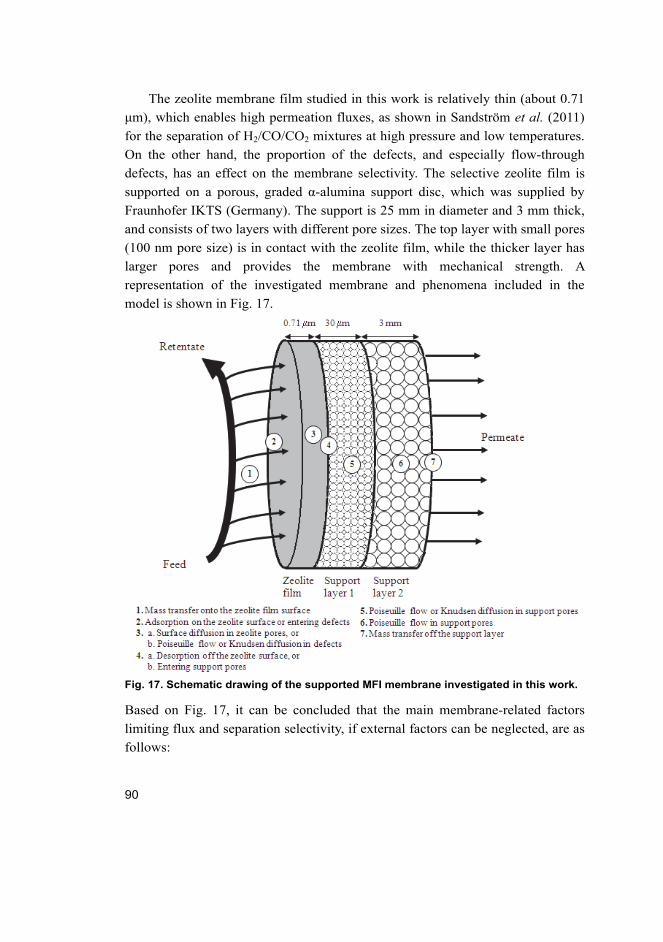
90
The zeolite membrane film studied in this work is relatively thin (about 0.71
μm), which enables high permeation fluxes, as shown in Sandström et al. (2011)
for the separation of H2/CO/CO2 mixtures at high pressure and low temperatures.
On the other hand, the proportion of the defects, and especially flow-through
defects, has an effect on the membrane selectivity. The selective zeolite film is
supported on a porous, graded α-alumina support disc, which was supplied by
Fraunhofer IKTS (Germany). The support is 25 mm in diameter and 3 mm thick,
and consists of two layers with different pore sizes. The top layer with small pores
(100 nm pore size) is in contact with the zeolite film, while the thicker layer has
larger pores and provides the membrane with mechanical strength. A
representation of the investigated membrane and phenomena included in the
model is shown in Fig. 17.
Fig. 17. Schematic drawing of the supported MFI membrane investigated in this work.
Based on Fig. 17, it can be concluded that the main membrane-related factors
limiting flux and separation selectivity, if external factors can be neglected, are as
follows:

91
– zeolite film adsorption behaviour,
– zeolite film diffusivity characteristics,
– film thickness,
– defects in the zeolite film, and
– support layer properties.
The key property of the Maxwell-Stefan formulation is the possibility to predict
multicomponent separation behaviour based only on pure component data. In
addition, the Maxwell-Stefan formulation can be extended to the description of
multicomponent permeation. These properties increase the number of applications
where Maxwell-Stefan based models can be utilized. The predictive capability of
the models has been demonstrated earlier, e.g. at low pressure for H2-CO2
mixtures with a supported high-silica MFI membrane (Wirawan et al. 2011). In
Paper I, a Maxwell-Stefan based model was created for a high-pressure separation
of H2-CO2 mixtures with a high-silica MFI membrane.
4.1.2 Pure component permeation
First, the pure component diffusivities were fitted based on the pure component
permeation measurements, as shown in Fig. 18 for H2 and in Fig. 19 for CO2. In
the case of H2, the literature data regarding adsorption on silicalite-1 was
observed to be scarce. Thus, the adsorption coefficient was fitted simultaneously
in Paper I. In addition, due to the low occupancy fraction of H2 in the conditions
under study, it was assumed that the surface diffusion of H2 follows the weak
confinement scenario, i.e. 0sH
sH 22
DD .

92
Fig. 18. Pure hydrogen permeation through the MFI membrane in experiments and
based on the model predictions. The pressure difference across the membrane was 1
bar and the temperature was 22°C. (Paper I, published by permission of Elsevier)
Fig. 18 shows that the model in Paper I is capable of predicting experimental
fluxes. However, it is worth noting that the experimental data in Fig. 18 is
scattered to a relatively great extent at low feed pressures. The most probable
origins of the scattering behaviour, i.e. other than experimental errors like
measurement and control of experimental conditions, are:
– impurities in the feed gas have accumulated during the experiments on the
zeolite film, thus blocking the permeation of H2 in later experiments,
– the hysteresis effect in adsorption of H2 on the zeolite. Müller and Unger
(1988) have noticed that the hysteresis behaviour occurs with different ZSM-
5 zeolites for nitrogen. Hence, the adsorption behaviour of a high-silica MFI
may be slightly different going first from low pressure to high pressure and
back to low pressure, or
– the zeolite film properties change slightly during the experiments due to some
irreversible processes like chemical reactions between H2 and zeolite.
Hence, the scattering may originate from a number of sources, which should be
investigated in more detail in the future work. The scattering induces uncertainty
to the estimated parameter values and the possibility of cross-correlation between
the estimated parameters. Nevertheless, it is important to note that both the fitted
5 10 15 20 25 30 35 40 451.2
1.3
1.4
1.5
1.6
1.7
1.8
Pfeed [bar]
NH
2 [m
ol s
-1 m
-2]
Experiments
Model

93
surface diffusivity and the Langmuir adsorption isotherm coefficient values were
in-line with the literature values as discussed in Paper I.
The permeation of CO2 was studied with two models in Paper I. In the first
model, the occupancy dependence was omitted. Thus, it was assumed that the
weak confinement scenario, Eq. (27) was applicable. In the second model, the
occupancy fraction dependence was included through the Reed-Ehrlich approach,
Eq. (30). Basically due to the high occupancy fraction of CO2 in the studied
conditions, the inclusion of the occupancy was demanded as discussed in Section
2.1.4. However, this was also tested in the given application.
Fig. 19. Pure CO2 permeation through an MFI membrane in experiments and using the
membrane model presented in Paper I either with occupancy dependence,
0sCO
sCO 22
DD , or without, 0sCO
sCO 22
DD . The temperature in the
experiments was between 20–22°C. (Paper I, published by permission by Elsevier).
As can be observed in Fig. 19, the application of the occupancy dependence did
not have a considerable effect on the fit of the model to the experimental data.
However, the value of the fitted surface diffusivity, 0sCO2
D , differs considerably
from the value obtained with the model including the occupancy dependence. To
investigate further which of the two models is more realistic, a comparison with
the literature models is shown in Fig. 20.
5 10 15 20 25 300
0.5
1
1.5
2
2.5
3
3.5
4
4.5
Pfeed [bar]
NC
O2 [
mol
s-1
m-2
]
DsCO2=Ds
CO2(0)
DsCO2Ds
CO2(0)
Exp. dP = 1 bar
Exp. dP = 2 bar
Exp. dP = 3 barExp. dP = 4 bar

94
Fig. 20. CO2 surface diffusivity as a function of the occupancy fraction of CO2.
Sandström et al. (2011), van den Broeke et al. (1999) and the present study models,
‘ 0sCO
sCO 22
DD ’ and ‘ 0sCO
sCO 22
DD ’, are based on experimental data.
Krishna and van Baten (2005, 2011) and Lee (2007) are based on molecular dynamics
simulation calculations. The temperature in all the references is in the range of 19–
27°C. (Paper I, published by permission by Elsevier).
As shown in Fig. 20, the estimated zero coverage surface diffusivity values of
both models in Paper I are well inside the range of the molecular dynamics
simulation values. In addition, the values are relatively close to the literature
values obtained from permeation experiments. On the other hand, according to
the MD simulations presented in Fig. 20, 0sCO2
D varies in the range of 129 sm105.55.4 . Hence, the fitted zero-coverage surface diffusivity
parameter value in the Reed-Ehrlich approach, Eq. (30), appears to be realistic in
the context. In contrast, the value of 0sCO2
D with the weak confinement scenario,
i.e. 0sCO
sCO 22
DD , is clearly below the corresponding values in MD
simulation studies in the literature. However, a final conclusion between the
models is not possible without further investigation.
4.1.3 Mixture separation
Finally, as both the surface diffusivity and adsorption behaviour of pure
components have been determined, the mixture separation can be predicted using
the models presented in Paper I. The results of the separation of an equimolar
0 0.1 0.2 0.3 0.4 0.5 0.6 0.7 0.8 0.9 10
1
2
3
4
5
6
7
8x 10
-9
CO2
Ds C
O2 [
m2 s
-1]
Krishna and van Baten (2011)Krishna and van Baten (2005)
Lee (2007)
Paper I, DsCO2Ds
CO2(0)
Paper I, DsCO2=Ds
CO2(0)
Sandström et al. (2011)van den Broeke et al. (1999)

95
H2/CO2 mixture with a supported MFI membrane at high feed pressure and low
temperatures are shown in Fig. 21.
Fig. 21. Model predictions and experimental fluxes of H2 and CO2 as a function of feed
pressure both with and without the occupancy dependence of sCO2
D .
feedperm 51 PP at a temperature of 23°C. Data is from Paper I.
Based on Fig. 21, it can be stated that the flux of hydrogen is slightly
underestimated at low pressure and slightly overestimated at high pressure with
both models. However, it is evident that adding the occupancy dependence of
CO2 and the effect of correlations for unary diffusion with Eq. (35) for both
components results in better prediction of the experimental component fluxes.
Usage of the dependence clearly decreases the flux of CO2, i.e. sCO2
D , at high
pressures, reflecting high occupancy fractions. At the same time, the smaller
surface diffusivity of CO2 decreases the diffusivity of H2 through the self-
exchange diffusivity term, sCO,CO 22
D , and naturally the binary exchange term, s, jiD .
Effects of the defects and the support
Even though the Maxwell-Stefan based models are predictive in nature, the
prediction of mixture separation also demands three important factors to be taken
into account:
5 10 15 20 25 300
0.5
1
1.5
2
2.5
3
3.5
4
4.5
5
Pfeed [bar]
Flu
x [m
ol s
-1 m
-2]
CO2, DsCO2Ds
CO2(0)
H2, DsCO2Ds
CO2(0)
CO2, DsCO2=Ds
CO2(0)
H2, DsCO2=Ds
CO2(0)
CO2 experiments
H2 experiments

96
– the effect of the flow-through defects on permeation,
– the effect of the support, and
– assumptions regarding external phenomena.
It is common in laboratory experiments that the majority of the membrane
external phenomena have only a minor effect. This is usually made possible by
designing the experiments appropriately. In contrast, the effects of the defects and
the support cannot be neglected if a predictive model is created. The magnitude of
the effects of the support and the flow-through defects can be observed in Fig. 22
and Fig. 23, respectively.
Fig. 22. Flux of CO2 with and without the support mass transfer resistance with
equimolar feed composition. Temperature is 23°C and feedperm 51 PP . (Paper I,
published by permission of Elsevier).
As can be seen in Fig. 22, the flux of CO2 is considerably slowed down by the
presence of the support, especially at low pressures. As shown in Paper I, the
support has a significant mass transfer resistance through the pressure gradient
across the support, which results in the trends shown in Fig. 22. The support also
causes the membrane selectivity to decrease, mainly due to the decrease of the
pressure gradient across the zeolite film, which also indirectly decreases the
chemical potential gradient across the zeolite film. Both the mass transfer and
5 10 15 20 25 30 35 401.5
2
2.5
3
3.5
4
4.5
5
5.5
NC
O2 [
mol
s-1
m-2
]
Pfeed [bar]
No support resistance
With support resistance

97
selectivity effects of the support decrease as the feed pressure increases. The
situation is the opposite with the defects as shown in Fig. 23.
Fig. 23. Component flux ratio at different feed pressures both with and without defects
in the zeolite film in the mixture separation conditions. Temperature is 23°C and
feedperm 51 PP . (Paper I, published by permission of Elsevier)
The curves showing the flux ratio with and without the defects diverge from each
other as a function of feed pressure, as shown in Fig. 23. Thus, the importance of
defects increases considerably as the feed pressure is increased. It can be
concluded that both the support and the defects have a considerable effect on
membrane behaviour and have to be included to enable the formulation of a
model with predictive capabilities.
4.2 Prediction of adsorption behaviour
4.2.1 Pure component
The usage of the knowledge of the Tff isat dependence of certain components
adsorption in the prediction of the temperature dependence of adsorption has been
limited in the literature. Even though the behaviour has been noticed in the
literature especially in the conjunction of the Polanyi theory, predicting the
adsorption behaviour at different temperatures using the vapour pressure
5 10 15 20 25 3011
12
13
14
15
16
17
NC
O2 /
NH
2
Pfeed [bar]
Without defects
With defects

98
temperature dependency has not been studied before the present work. The
behaviour is illustrated in the case of water adsorption in Fig. 24 for a 4A zeolite
and in Fig. 25 for a silicalite-1 zeolite.
a)
b)
Fig. 24. Adsorbed loading of water vapour on zeolite 4A as a function of a) the system
pressure and b) sat
iPP based on the experimental data presented in Gorbach et al.
(2004).
10-4
10-2
100
102
0
0.02
0.04
0.06
0.08
0.1
0.12
0.14
0.16
0.18
0.2
P [mbar]
q [k
g/kg
]
T = 0 oC
T = 25 oC
T = 61 oC
T = 101 oC
10-6
10-5
10-4
10-3
10-2
10-1
0
0.02
0.04
0.06
0.08
0.1
0.12
0.14
0.16
0.18
0.2
P/Psati
q [k
g/kg
]
T = 0 oC
T = 25 oC
T = 61 oC
T = 101 oC

99
a)
b)
Fig. 25. Adsorbed loading of water vapour on silicalite-1 (OH-) as a function of a) the
system pressure and b) sat
iPP based on the experimental data presented in Zhang et
al. (2012).
As can be seen in Fig. 24 and Fig. 25, the application of the satiPP dependence
results in the overlapping of water loading data at different temperatures.
Therefore, in Paper IV, the temperature dependence of vapour pressure was
applied successfully in the description of adsorption on different zeolites. Thus,
on the basis of Fig. 24, Fig. 25 and Paper IV it can be concluded that especially
for water and alcohols, the temperature dependence of adsorption on zeolites can
be described with vapour pressure temperature dependence. It is worth noting that,
essentially, the saturation loading is not a function of temperature. However, it is
common to fit the saturation loading for each temperature separately in the
0 0.02 0.04 0.06 0.08 0.1 0.12 0.140
0.5
1
1.5
2
2.5
P [bar]
q [m
ol/k
g]
T = 25 oC
T = 35 oC
T = 45 oC
T = 55 oC
0 0.1 0.2 0.3 0.4 0.5 0.6 0.7 0.8 0.9 10
0.5
1
1.5
2
2.5
P/Psati
q [m
ol/k
g]
T = 25 oC
T = 35 oC
T = 45 oC
T = 55 oC

100
literature (see e.g. Loughlin 2009). This can be avoided in multiple applications
with the application of the satiP temperature dependence (Paper IV ). The sat
iP
temperature dependence approach can be applied to any adsorption isotherm
model by simply replacing if with satii Pf , i.e. ii fq is replaced with
satiii Pfq , as shown in Paper IV. In addition, as the first guess, the
temperature dependence of all other adsorption parameters, i.e. typically Tbi ,
can be neglected after the replacement. The practical implementation of the satiP
temperature dependence approach is also easy due to the wide availability of
vapour pressure data in the literature, and principally only adsorption data at one
temperature is demanded to predict the adsorption behaviour at any temperature.
The main practical limit of the approach with respect to temperature is the
validity range of the vapour pressure. This is especially true if supercritical
conditions are studied. However, on the whole, the approach is a valuable tool
from the perspective of engineering work, as concluded in Paper IV.
4.2.2 Mixture
The satiP temperature dependence approach can be applied to the description of
mixture adsorption in conjunction with the appropriate mixture adsorption model.
The basic idea is to fit adsorption parameters at one temperature for each
component with a suitable pure component adsorption isotherm, applying the sat
ii Pf ratio. It is then assumed that data regarding the temperature dependence
of adsorption, e.g. the heat of adsorption, is not available, or the measurement is
not possible within the available time frame for the studied system. Then the
multicomponent adsorption is predicted (at another temperature) with an
appropriate multicomponent adsorption model, e.g. the multicomponent
Langmuir isotherm, IAST, PRAST or RAST.
The usage of the approach to predict mixture adsorption is illustrated with
water-ethanol vapour mixture adsorption on an NaA zeolite. The vapour mixture
can be assumed to behave ideally, thus satsatiii PPPf . Thus, applying the
vapour pressure temperature dependence, and using the Langmuir adsorption
isotherm as the base model, the following modified Langmuir model is applied to
describe the pure component adsorption (Paper II ):

101
TP
Pb
TP
Pb
ii
ii
i
sat
satsati
1
, (81)
where ib is the temperature-independent adsorption equilibrium parameter. The
pure component adsorption parameters have been fitted at 305 K, whereas the
mixture adsorption is predicted at 333 K. The fitted pure component adsorption
parameters are presented in Paper II (see Table 4 in Paper II ). The fit of the
model to water and ethanol adsorption data is shown in Fig. 26.
Fig. 26. Pure water and ethanol adsorption on NaA at 305 K predicted by the modified
Langmuir model, ‘Model’. Experimental data, ‘Exp’, is from Pera-Titus et al. (2008).
As can be seen in Fig. 26, the modified Langmuir model describes the adsorption
of pure water and ethanol on NaA at 305 K well. Now, let us compare the
prediction of mixture adsorption at 333 K with different models. The results with
different mixture adsorption models are shown in Fig. 27.
0 0.05 0.1 0.15 0.2 0.25 0.3 0.35 0.4 0.45 0.50
2
4
6
8
10
12
P/Pisat
q [m
ol k
g-1]
Water, Exp
Water, ModelEtOH, Exp
EtOH, Model

102
a)
b)
Fig. 27. a) Water and b) ethanol mixture adsorption loadings on NaA at 333 K and 2.1
kPa based on the experiments, IAST model predictions both with the vapour pressure
temperature dependence approach and without temperature dependence (Paper II ),
and PRAST model predictions. The experimental data is taken from Pera-Titus et al.
(2008).
As can be seen in Fig. 27, the models with vapour pressure temperature
dependence predict the adsorbed loadings relatively well. In contrast, IAST
0 0.1 0.2 0.3 0.4 0.5 0.6 0.7 0.8 0.9 10
2
4
6
8
10
12
yw ater
q wat
er [
mol
kg-1
]Experiments
IAST with T-dependence
IAST no T-dependence
PRAST with T-dependence
0 0.1 0.2 0.3 0.4 0.5 0.6 0.7 0.8 0.9 10
0.5
1
1.5
2
2.5
3
3.5
yw ater
q EtO
H [
mol
kg-1
]
Experiments
IAST with T-dependenceIAST no T-dependence
PRAST with T-dependence

103
without temperature dependence clearly over-predicts the loading of water and
under-predicts the loading of ethanol. The best selectivity predictions as a whole
can be achieved by using PRAST. In Fig. 27, the differences between the
predictions of different mixture adsorption models are partly, i.e. in addition to the
temperature dependence, caused by the different formulation of the respective
models. Based on Fig. 27 and Paper II, it can be concluded that the satiP
temperature dependence approach is a feasible approach in the description of pure
component adsorption and reasonably good mixture adsorption predictions can be
achieved using the approach in conjunction with an appropriate mixture
adsorption model.
4.3 Prediction of phase stability
The prediction of phase stability can be performed by finding all the stationary
points of the tangent plane distance function (TPDF). The stationary points can be
found by solving Eqs. (54)-(55). Eqs. (54)-(55) form a non-linear equation set,
which can be solved with homotopy methods applied in Papers III and V.
4.3.1 Finding the first root
The main peculiarity of TPDF is that one solution of the problem, i.e. the trivial
root, is known in advance. This property of the TPDF problem distinguishes it
from other process models, and related numerical problems that exhibit multiple
solutions. The trivial root is a major problem for both local and global solution
methods, which concentrate on finding only the first root of a problem. The
importance of the issue in the context of TPDF problem solving, Eqs. (52) and
(53), can be viewed in Table 8.

104
Table 8. The proportion [%] of first root types with Newton modified bounded
homotopy, Eq. (63), and fsolve routine of Matlab for Case 3 presented in Paper V with
starting point restriction. 1000 randomly (with the rand function of Matlab) selected
starting points were studied. The mixture under investigation was z = [0.29989,
0.20006, 0.50005].
Root Homotopy fsolve routine of Matlab
Isola1 13.7 -
Trivial (Local minimum) 13.4 48.1
Saddle point 42.4 51.7
Global minimum 13.5 0.2
Unfeasible 0.1 -
No root2 16.9 - 1 No root found, a starting point isola detected, 2 No root, the path crosses. θ = −20.
As can be seen in Table 8, the trivial root is found with a high probability as a first
root with both Newton modified bounded homotopy, i.e. Eq. (63) with Newton
homotopy, and the local solver of Matlab. With a homotopy this is not so
detrimental, as the homotopy path can be tracked forward after the first root has
been found. In contrast, with the local solver a new starting point has to be
selected to find a new root, and even then it is possible to end up with the same
root. The main distinctive drawbacks of different modified bounded homotopies,
Eq. (63), in finding the first root of TPDF solution are (Paper V ):
– with the affine homotopy function, unfeasible roots are frequently obtained as
the first root,
– with the fixed-point homotopy function, some of the roots are unattainable as
the first root regardless of the starting point, and
– with the Newton homotopy function, no roots are found due to the frequent
appearance of starting point isolas and multiplicities.
However, in the cases studied in Paper V, the unattainable roots were classified as
saddle points, not as the global minimum or local minima. Hence, this is not
detrimental with respect to the overall solving progress. The unfeasible roots,
fortunately, are easily separated from feasible roots, as they do not fulfil the
original TPDF equation set, Eqs. (54) and (55). In contrast, the appearance of a
starting point isola cannot be circumvented with the Newton modified bounded
homotopy Eq. (63). The drawbacks stated can be tackled e.g. by

105
1. selecting a new starting point,
2. selecting another homotopy,
3. modifying the problem equation set,
4. modifying the homotopy, or
5. using knowledge of the location of the trivial root.
The first two options are self-evident alternatives applicable to the solution of any
problem, whereas the third option of modifying the problem equation set demands
more knowledge of the problem properties.
Especially due to the appearance of starting point isolas with the Newton
homotopy function and the study of the attraction domain maps of the first root
for different homotopies, the following solution strategy was proposed in Paper V:
– use modified bounded fixed-point homotopy, in particular, if the trivial root is
a saddle point,
– start the solution sequentially from each vertex point of the composition
domain, and
– track the homotopy paths until the first root is obtained.
However, as acknowledged in Paper V, the proposed solution strategy can only
verify the phase stability/instability of a liquid mixture into several liquid phases
along with feasible initial estimates for the subsequent phase splitting calculation
with a high degree of certainty, not robustly. Thus, the fourth (modify the
homotopy) and fifth (use the trivial root) alternatives should be investigated
further. The utilization of the trivial root to our advantage is discussed next. The
combined effect of utilizing the trivial root and the modification of the homotopy
to create a more robust solving method is studied later on in Section 4.3.3.
4.3.2 Utilization of the trivial root of TPDF
The starting point isola that is formed can be circumvented by continuing path
tracking from the trivial root after the isola has been obtained. In this situation,
the starting point and the trivial root are on different homotopy branches, as can
be seen in Fig. 28.

106
Fig. 28. Homotopy branches with the Newton modified bounded homotopy, Eq. (63), in
the component system of toluene-water-aniline (see Case 3 of Paper V ). The starting
point is 17.003.080.00 x .
The option of continuing from the trivial root after noticing that a starting point
isola has appeared adds complexity to the resulting solving algorithm. In addition,
the solving algorithm is still dependent on the starting point selection as
continuing from the trivial root cannot guarantee that all the feasible roots are on
the same homotopy branch. Thus, other options should also be investigated.
Therefore, the modification of the homotopy is discussed next.
4.3.3 Modification of the bounded homotopy
The homotopy can be modified by introducing homotopy parameter bounding, Eq.
(65). The bounding can be utilized both to connect separate homotopy branches
and disconnect homotopy branches. In the case of a starting point isola being
formed, the application of homotopy parameter bounding can be used to break the
isola. This is illustrated in Fig. 29.
-2 -1 0 1 2 3
0
0.5
1
0
0.2
0.4
0.6
0.8
1
xtoluene
x wat
er
Starting pointTrivial root
Feasible roots
Starting point multiplicity
Isola branchSolution branch

107
Fig. 29. Homotopy path with the Newton modified bounded homotopy with, Eq. (65)
and without homotopy parameter bounding, Eq. (63), in a mapped variable space,
indicated with ‘Bounded path’ and ‘Unbounded path’ respectively. The starting point is
4685.02218.13979.0inf0 x . 001.0M . The case is Case 3 of Paper V.
As can be seen in Fig. 29, the application of homotopy parameter bounding
breaks the isola and the homotopy path that is formed travels through one of the
original problem roots. However, the two other feasible roots are not obtained.
This is the principal problem with Newton bounded homotopy, Eq. (65),
combining both variable and homotopy parameter bounding. It is also worth
noting that bounding the homotopy path to travel within a defined x, domain
is not possible. However, by selecting a suitable value for parameter M , it can be
ascertained that the path will exit the domain with respect to the homotopy
parameter. In addition, the formed path is continuous if both the variables and the
homotopy parameter are bounded.
As originally presented in Paper III, bounded homotopies can be modified to
form a homotopy path that is continuous and also to include all the feasible roots
of a TPDF problem. The bounding of the homotopy parameter is used to connect
the separate homotopy branches. It is worth noting that in all the cases presented
-2-1
01
2-10
-50
5
-10
-8
-6
-4
-2
0
2
4
xinftoluene
xinf
wat
er
Feasible root
Starting point
Unbounded path
Bounded path

108
in Paper III the value of M was set to 0.001. The performance of the homotopy,
Eq. (66), is illustrated in Fig. 30.
Fig. 30. The homotopy path with the trivial root utilizing Newton modified homotopy,
Eq. (66) in the component system of toluene-water-aniline (see Case 3 of Paper V ). 91051 iu and
9105 il . 001.0M .
As can be seen in Fig. 30, all the feasible roots are found from a single starting
point. In the studied component system, the global minimum exists close to the
feasible problem domain boundaries. When mole fractions close to 0 and/or 1
exist, the upper and lower constraints must be defined so that the feasible
solutions do not fall in the bounding zone, i.e. the width of the bounding zone
should be narrow.
-1.5-1
-0.50
0.51
1.5
0
0.5
1
0
0.1
0.2
0.3
0.4
0.5
0.6
0.7
0.8
0.9
1
xtoluene
x wat
er
Trivial root
Feasible roots
Homotopy path

109
Fig. 31. Homotopy path with the trivial root utilizing Newton modified homotopy, Eq.
(66) in mapped variable space in the component system of toluene-water-aniline (see
Case 3 of Paper V ) 8inf iu and 8inf il . 001.0M .
Fig. 31 shows that the homotopy path intercepts the 1 and 1 planes at
the points where the variables have the same values as the opposite signs, i.e. at
the points 995.8858.81;995.8858.81, infexit,exit x . It is important to
note that the interception takes place inside the bounding zone where both the
homotopy parameter and variables bounding features are in force. On the other
hand, the interception locations of the homotopy path enable the alternative of
continuing path tracking in the same direction from inf,exitexit , x instead of
starting again from inf,0 z backwards.
Finally, it is possible to evaluate the consistency of the obtained roots
according to the values presented in Table 9 with the topology criterion of
Wasylkiewicz et al. (1996).
-1.5-1
-0.500.5
11.5
-10
-5
0
5
10
-10
-5
0
5
10
xinftoluene
xinf
wat
er
Trivial root
Feasible roots
Interception at = -1 and = 1
Homotopy path
x inf = [8.858 -8.995]
x inf = [-8.858 8.995]

110
Table 9. The feasible stationary points and corresponding values of D for toluene (1) –
water (2) – aniline (3) composition z = [0.29989, 0.20006, 0.50005]. (Paper V, published
by permission of ACS Publications)
Root, [x1 x2 x3] Type D
0.29989 0.20006 0.50005 Trivial, Local minimum 0
0.29255 0.209041 0.498409 Saddle point (odd) 2.9698·10-7
6.6937·10-5 0.996865 3.068·10-3 Global minimum -0.29454
As shown in Table 9, 2d , max 0N , min 2N , evensad 0N and odd
sad 1N . Thus, even odd
max min sad sad 1N N N N . Hence, according to the topology criterion, Eq. (57),
the number of stationary points is consistent. Although the criterion only yields
knowledge of the consistency of the relative number of stationary points, in Paper
III it was demonstrated that the proposed solution strategy was able to find all the
feasible stationary points in all the cases studied. In addition, the topology
criterion was fulfilled in all the cases. The mixture under investigation is unstable
in the given conditions and splits into two liquid phases as shown in Table 10.
Table 10. LLE compositions and phase fractions for toluene (1) – water (2) – aniline (3)
composition z = [0.29989, 0.20006, 0.50005]. At a temperature of 295 K and P = 1 atm.
(Paper V, published by permission of ACS Publications)
Liquid phase Phase fraction L, [x1 x2 x3]
L1 0.86485 0.34674 0.07584 0.57742
L2 0.13515 9.13·10-5 0.9949475 4.9612·10-3
As can be noticed by comparing Table 9 and Table 10, the global minimum
composition is the composition of one of the resulting liquid phases. Thus, LLE
solving can be initiated efficiently based on phase stability analysis solutions.
This can be performed even with a local solving method, for instance, due to the
close proximity of the initial guess and the solution of the LLE equation set.

111
5 Conclusions and suggestions for future research
As illustrated in Papers I, III and V, the formulation of a predictive process model
demands both a robust solving strategy and a process model with a firm
phenomenon base. The robustness of the solving strategy can be improved either
by extensively applying problem-dependent knowledge (Paper I) or by utilizing a
global solving method (Papers III and V).
However, the usage of a global solving method without any exploitation of
the problem properties cannot guarantee that all the feasible solutions are found.
Rather, as shown in Paper III, finding all the feasible solutions of the phase
stability analysis problem robustly also requires the utilization of the trivial root
of the problem. The trivial root of a phase stability analysis problem is a special
case among the class of process models. Generally, no solutions of the process
model are known before the start of the solution. It is common that both the local
solving methods and the modified bounded homotopies presented by Malinen and
Tanskanen (2008) find the trivial root first, as shown in Paper V, for multiple
liquid-liquid phase equilibrium cases. On the other hand, finding all the feasible
solutions necessitates modifying the existing modified bounded homotopies
presented by Malinen and Tanskanen (2008, 2010) appropriately. For that purpose,
a combination of variables and homotopy parameter bounding features was
utilized for the first time (Paper III ).
Finding all the feasible solutions of a process model robustly is an ambitious
goal especially when applied to a general process model. There is as yet no tool
for the purpose. However, the application of the solution strategy proposed in
Paper III has yielded promising results in the endeavours towards this goal.
Therefore, the solution strategy should be applied to a wider class of process
models. If the same concept as that in Paper III could be applied in the solution of
the models, it would undoubtedly be extremely useful in the field of process
systems engineering.
Formulation of a predictive process model in connection with membrane
separation can be achieved with the Maxwell-Stefan approach. Usage of the
Maxwell-Stefan approach means that pure component surface diffusivities and
binary exchange diffusivities are used to predict multicomponent membrane
separation. However, the accuracy of the predictions is dependent on the adopted
model for pure component surface diffusion and the underlying assumptions
performed regarding the adsorption phenomena characteristics. In Paper I, it was

112
illustrated that the experimental H2/CO2 separation data at high pressure can be
predicted well on the basis of pure component permeation data and adsorption
data. However, prediction results are considerably dependent on the self-exchange
and binary exchange correlations used. Similarly, prediction of mixture
adsorption demands the usage of a suitable predictive model. Adsorbed solution
theory models were applied successfully for this purpose in Papers I and II.
Further studies should include the rigorous application of the occupancy
fraction dependence of surface diffusion to verify its general applicability in
conjunction with experimental data. The verification of the correct occupancy
dependence demands experimental data from a wide occupancy fraction domain,
i.e. from low to high fugacity/pressure. This data is not generally available for
many adsorbate-adsorbent pairs. Similarly, no comprehensive description exists
for the correlation of self-exchange and binary exchange surface diffusivities.
Molecular dynamics simulation appears to be a feasible tool for determining
surface diffusivities in membrane separation based on pure component
permeation data as shown in Paper I. Thus, MD simulation could be used as a
predictive method to predict ‘real’ surface diffusivity behaviour. Therefore, the
application of an MD-based surface diffusivity and adsorption behaviour more
widely in the description of both adsorption and surface diffusion on zeolites
could be beneficial to the overall progress of membrane research. Even though
the usage of MD also definitely has particular uncertainties, such as how in
practice a high-silica MFI instead of silicalite-1 can be treated with MD, these
limits should be sought in future research.
In conclusion, it can be stated that the combination of a model with a clear
phenomenon base and a robust solution strategy results in the improvement of the
predictive capabilities of the investigated separation process models. In addition,
the usability of the models in separation process design is enhanced.

113
References
Allgower E & Georg K (1980) Simplicial and Continuation Methods for Approximating Fixed Points and Solutions to Systems of Equations. SIAM Rev 22: 28–85.
Aslam N & Sunol AK (2006) Sensitivity of azeotropic states to activity coefficient model parameters and system variables. Fluid Phase Equilibr 240: 1–14.
Baerlocher C, McCusker LB & Olson, DH (2007) Atlas of zeolite framework types, sixth ed., Elsevier B.V., Amsterdam.
Baker LE, Pierce AC & Luks KD (1982) Gibbs Energy Analysis of Phase Equilibria. Soc Pet Eng J 22: 731–742.
Bakker WJ, van den Broeke LJP, Kapteijn F & Moulijn J (1997) Temperature dependence of one-component permeation through a silicalite-1 membrane. AIChE J 43: 2203–2214.
Balogh J, Csendes T & Stateva RP (2003) Application of a stochastic method to the solution of the phase stability problem: cubic equations of state. Fluid Phase Equilibr 212: 257–267.
Bausa J & Marquardt W (2000) Quick and reliable phase stability test in VLLE flash calculations by homotopy continuation. Comput Chem Eng 24: 2447–2456.
Bekiaris N, Meski GA & Morari M (1996) Multiple steady states in heterogeneous azeotropic distillation. Ind Eng Chem Res 35: 207–227.
Bhargava V, Fateen SEK & Bonilla-Petriciolet A (2013) Cuckoo Search: A new nature–inspired optimization method for phase equilibrium calculations. Fluid Phase Equilibr 337: 191–200.
Biegler LT, Grossmann IE & Westerberg AW (1997) Systematic methods of chemical process design. Prentice-Hall, Inc. ISBN: 0-13-492422-3.
Bonilla-Petriciolet A, Vázquez-Roman R, Iglesias-Silva GA & Hall KR (2006) Performance of Stochastic Global Optimization Methods in the Calculation of Phase Stability Analyses for Nonreactive and Reactive Mixtures. Ind Eng Chem Res 46: 4764–4772.
Cairns BP & Furzer IA (1990) Multicomponent Three-Phase Azeotropic Distillation. 2. Phase-Stability and Phase-Splitting Algorithms. Ind Eng Chem Res 29: 1364–1382.
Do DD (1998) Adsorption analysis: equilibria and kinetics. Imperial College Press, London.
Do DD & Do HD (1997) A new adsorption isotherm for heterogeneous adsorbent based on the isosteric heat as a function of loading. Chem Eng Sci 52: 297–310.
Eckert E & Kubicek M (1997) Computing heterogeneous azeotropes in multicomponent mixtures. Comput Chem Eng 21: 347-350.
Englezos P & Kalogerakis N (2001) Applied parameter estimation for chemical engineers. Marcel Dekker Inc, New York. ISBN: 0-8247-9561-X.
Erto A, Lancia A & Musmarra D (2011) A modelling analysis of PCE/TCE mixture adsorption based on Ideal Adsorbed Solution Theory. Sep Purif Technol 80: 140–147.

114
Fateen SEK, Bonilla-Petriciolet A & Rangaiah GP (2012) Evaluation of covariance matrix adaptation evolution strategy, shuffled complex evolution and firefly algorithms for phase stability, phase equilibrium and chemical equilibrium problems. Chem Eng Res Des 90: 2051–2071.
Fidkowski ZT, Malone MF & Doherty MF (1993) Computing azeotropes in multicomponent mixtures. Comput Chem Eng 17: 1141–1155.
Finlayson BA (1980) Nonlinear analysis in chemical engineering. McGraw-Hill Inc. Gamba G, Rota R, Storti G, Carra S & Morbidelli M (1989) Adsorbed solution theory
models for multicomponent adsorption equilibria. AIChE J 35: 959–966. Gecegormez H & Demirel Y (2005) Phase stability analysis using interval Newton method
with NRTL model. Fluid Phase Equilibr 237: 48–58. Hangzhou W, Zhihong Y, Bingzhen C, Xiaorong H, Jinsong Z & Tong Q (2011) Analysis
of the stability and controllability of chemical processes. Comput Chem Eng 35: 1101–1109.
Harlick PJE & Tezel FH (2003) Adsorption of carbon dioxide, methane and nitrogen: pure and binary mixture adsorption for ZSM–5 with SiO2/Al2O3 ratio of 280. Sep Purif Technol 33: 199–210.
Hedlund J, Korelskiy D, Sandström L & Lindmark J (2009) Permporometry analysis of zeolite membranes. J Memb Sci 345: 276-287.
Helminen J, Helenius J, Paatero E & Turunen I (2000) Comparison of sorbents and isotherm models for NH3-gas separation by adsorption. AIChE J 46: 1541–1555.
Hua JZ, Brennecke JF & Stadtherr MA (1996) Reliable Prediction of Phase Stability Using an Interval Newton Method. Fluid Phase Equilibr 116: 52–59.
Hua JZ, Brennecke JF & Stadtherr MA (1998) Enhanced Interval Analysis for Phase Stability: Cubic Equation of State Models. Ind Eng Chem Res 37: 1519–1527.
Jalali F, Seader JD & Khaleghi S (2008) Global solution approaches in equilibrium and stability analysis using homotopy continuation in the complex domain. Comput Chem Eng 32: 2333–2345.
Jalali-Farahani F & Seader JD (2000) Use of homotopy-continuation method in stability analysis of multiphase, reacting systems. Comput Chem Eng 24: 1997–2008.
Jalali F & Seader JD (1999) Homotopy continuation method in multi-phase multi-reaction equilibrium systems. Comput Chem Eng 23: 1319–1331.
Kannan A, Joshi MR, Reddy GR, Shah DM (2005) Multiple-Steady-States identification in homogeneous azeotropic distillation using a process simulator. Ind Eng Chem Res 44: 4386–4399.
Kangas J, Ahola J, Maunula T, Korpijärvi J & Tanskanen J (2002) Automotive exhaust gas converter model for warm–up conditions. 17th International Symposium on Chemical Reaction Engineering, Hong Kong, China.
Kapteijn F, Moulijn JA & Krishna R (2000) The generalized Maxwell–Stefan model for diffusion in zeolites: sorbate molecules with different saturation loadings. Chem Eng Sci 55: 2923–2930.
Khaleghi S & Jalali F (2007) Multiple Solutions in Stability Analysis Using Homotopy Continuation in Complex Space. Chem Eng Commun 194: 1241–1258.

115
Kienle A, Groebel M & Gilles ED (1995) Multiple steady states in binary distillationtheoretical and experimental results. Chem Eng Sci 50: 2691–2703.
Krishna R (1990) Multicomponent surface diffusion of adsorbed species: A description based on the generalized Maxwell–Stefan Equations. Chem Eng Sci 45: 1779–1791.
Krishna R & Baur R (2003) Modelling issues in zeolite based separation processes. Sep Purif Technol 33: 213–254.
Krishna R & Baur R (2004) Analytic solution of the Maxwell–Stefan equations for multicomponent permeation across a zeolite membrane. Chem Eng J 97: 37–45.
Krishna R & Paschek D (2000) Separation of hydrocarbon mixtures using zeolite membranes: a modelling approach combining molecular simulations with the Maxwell–Stefan theory. Sep Purif Technol 21: 111–136.
Krishna R & Paschek D (2002) Self–diffusivities in multicomponent mixtures in zeolites. Phys Chem Chem Phys 4: 1891–1898.
Krishna R, Paschek D & Baur R (2004) Modeling the occupancy dependence of diffusivities in zeolites. Micropor Mesopor Mater 76: 233–246.
Krishna R & van Baten JM (2005) Kinetic Monte Carlo Simulations of the Loading Dependence of Diffusion in Zeolites. Chem Eng Technol 28: 160–167.
Krishna R & van Baten JM (2009) Unified Maxwell-Stefan description of binary mixture diffusion in micro- and meso-porous materials. Chem Eng Sci 64: 3159–3178.
Krishna R & van Baten JM (2010a) Hydrogen bonding effects in adsorption of water–alcohol mixtures in zeolites and the consequences for the characteristics of the Maxwell–Stefan diffusivities. Langmuir 26: 10854–10867.
Krishna R & van Baten JM (2010b) Highlighting pitfalls in the Maxwell–Stefan modelling of water-alcohol mixture permeation across pervaporation membranes. J Memb Sci 360: 476–482.
Krishna R & van Baten JM (2010c) Mutual slowing-down effects in mixture diffusion in zeolites. J Phys Chem C 114: 13154–13156.
Krishna R & van Baten JM (2011) Maxwell–Stefan modeling of slowing–down effects in mixed gas permeation across porous membranes. J Memb Sci 383: 289–300.
Lee SC (2007) Prediction of permeation behavior of CO2 and CH4 through silicalite–1 membranes in single–component or binary mixture systems using occupancy–dependent Maxwell–Stefan diffusivities. J Memb Sci 306: 267–276.
Lito PF, Santiago AS, Cardoso SP, Figueiredo BR & Silva CM (2011) New expressions for single and binary permeation through zeolite membranes for different isotherm models. J Memb Sci 367: 21–32.
Loughlin KF (2009) Water isotherm models for 4A (NaA) zeolite. Adsorption 15: 337–353. Lucia A, DiMaggio PA, Bellows ML & Octavio LM (2005) The phase behavior of n-
alkane systems. Comput Chem Eng 29: 2363–2379. Luyben WL (1996) Process modeling, simulation, and control for chemical engineers. 2nd
ed. McGraw-Hill, New York. Malek A & Farooq S (1996) Comparison of isotherm models for hydrocarbon adsorption
on activated carbon. AIChE J 42: 3191–3201.

116
Malinen I (2010) Improving the robustness with modified bounded homotopies and problem-tailored solving procedures. Acta Univ. Oul. C 377. ISBN 978-951-42-9337-5.
Malinen I & Tanskanen J (2008) Modified bounded homotopies to enable a narrow bounding zone. Chem Eng Sci 63: 3419–3430.
Malinen I & Tanskanen J (2009) Thermally coupled side–column configurations enabling distillation boundary crossing. 1. An overview and a solving procedure. Ind Eng Chem Res 48: 6387–6404.
Malinen I & Tanskanen J (2010) Homotopy parameter bounding in increasing the robustness of homotopy continuation methods in multiplicity studies. Comput Chem Eng 34: 1761–1774.
Mason EA & Malinauskas AP (1983) Gas transport in porous media: The Dusty-Gas Model. Elsevier Science Publishers B.V., Amsterdam, The Netherlands. ISBN 0-444-42190-4.
McDonald CM & Floudas CA (1995a) Global Optimization for the Phase Stability Problem. AIChE J 41: 1798–1814.
McDonald CM & Floudas CA (1995b) Global Optimization for the Phase and Chemical Equilibrium Problem: Application to the NRTL Equation. Comput Chem Eng 19: 1111–1139.
McDonald CM & Floudas CA (1997) GLOPEQ: A New Computational Tool for the Phase and Chemical Equilibrium Problem. Comput Chem Eng 21: 1–23.
Michelsen ML (1982) The isothermal flash problem. Part I: Stability. Fluid Phase Equilibr 9: 1–19.
Michelsen ML & Mollerup JM (2007) Thermodynamic models: fundamentals & computational aspects. Tie-line publications. 2nd ed. ISBN: 87-989961-3-4.
Monsalvo MA & Shapiro AA (2007) Modeling adsorption of binary and ternary mixtures on microporous media. Fluid Phase Equilibr 254: 91–100.
Müller U & Unger KK (1988) Sorption studies on large ZSM-5 crystals: The influence of aluminium content, the type of exchangeable cations and the temperature on nitrogen hysteresis effects. Stud Surf Sci Catal 39: 101–108.Myers AL & Prausnitz JM (1965) Thermodynamics of Mixed-Gas Adsorption. AIChE J 11: 121–127.
Nichita DV & Gomez S (2009) Efficient location of multiple global minima for the phase stability problem. Chem Eng J 152: 251–263.
Nichita DV, Gomez S & Luna E (2002) Multiphase equilibria calculation by direct minimization of Gibbs free energy with a global optimization method. Comput Chem Eng 26: 1703–1724.
Paloschi JR (1995) Bounded Homotopies to Solve Systems of Algebraic Nonlinear Equations. Comput Chem Eng 19: 1243–1254.
Paloschi JR (1997) Bounded Homotopies to Solve Systems of Sparse Algebraic Nonlinear Equations. Comput Chem Eng 21: 531–541.
Poling BE, Prausnitz JM & O’Connell JP (2001) The properties of gases and liquids. McGraw-Hill Companies. 5th ed. ISBN 0-07-011682-2.

117
Rangaiah GP (2001) Evaluation of genetic algorithms and simulated annealing for phase equilibrium and stability problems. Fluid Phase Equilibr 187–188: 83–109.
Romanainen J (1994) Numerical strategies in solving gas–liquid reactor models. Dissertation. Åbo Akademi. ISBN 951-650-379-9.
Ruthven DM (1984) Principles of adsorption and adsorption processes. John Wiley & Sons, Inc. ISBN 0-471-86606-7.
Sakuth M, Meyer J & Gmehling J (1998) Measurement and prediction of binary adsorption equilibria of vapors on dealuminated Y–zeolites (DAY). Chem Eng Process 37: 267–277.
Sandström L, Lindmark J & Hedlund J (2010) Separation of methanol and ethanol from synthesis gas using MFI membranes. J Memb Sci 360: 265–275.
Sandström L, Sjöberg E & Hedlund J (2011) Very high flux MFI membrane for CO2 separation. J Memb Sci 380: 232–240.
Seader JD, Kuno M, Lin W-J, Johnson SA, Unsworth K & Wiskin JW (1990) Mapped continuation methods for computing all solutions to general systems of nonlinear equations. Comput Chem Eng 14: 71–85.
Seider WD, Seader JD & Lewin DR (1999) Process design principles: synthesis, analysis, and evaluation. ISBN: 0-471-24312-4.
Sircar S & Myers AL (2003) Gas separation by zeolites. In: Auerbach SM, Carrado KA & Dutta PK (eds) Handbook of zeolite science and technology. Marcel Dekker, Inc: 1063–1104.
Shacham M & Brauner N (2002) Numerical solution of non-linear algebraic equations with discontinuities. Comput Chem Eng 26: 1449–1457.
Shapiro AA & Stenby EH (2002) Multicomponent adsorption: principles and models. In: Tóth J (ed) Adsorption: theory, modelling, and analysis. Marcel Dekker, Inc: 375–431.
Skoulidas AI & Sholl DS (2002) Transport diffusivities of CH4, CF4, He, Ne, Ar, Xe, and SF6 in silicalite from atomistic simulations. J Phys Chem B 106: 5058–5067.
Skoulidas AI, Sholl DS & Krishna R (2003) Correlation effects in diffusion of CH4/CF4 mixtures in MFI Zeolite. A study linking MD simulations with the Maxwell–Stefan formulation. Langmuir 19: 7977–7988.
Sochard S, Fernandes N & Reneaume J-M (2010) Modeling of Adsorption Isotherm of a Binary Mixture with Real Adsorbed Solution Theory and Nonrandom Two-Liquid Model. AIChE J 56: 3109–3119.
Sofyan Y, Ghajar AJ & Gasem KAM (2003) Multiphase equilibrium calculations using Gibbs minimization techniques. Ind Eng Chem Res 42: 3786–3801.
Srinivas M & Rangaiah GP (2007) A study of differential evolution and tabu search for benchmark, phase equilibrium and phase stability problems. Comput Chem Eng 31: 760–772.
Staudt PB, Cardozo NSM & Soares RP de (2013) Phase stability analysis using a modified affine arithmetic. Comput Chem Eng 53: 190–200.
Sun AC & Seider WD (1995) Homotopy-continuation method for stability analysis in the global minimization of the Gibbs free energy. Fluid Phase Equilibr 103: 213–249.

118
Talu O & Myers AL (1988) Rigorous thermodynamic treatment of gas adsorption. AIChE J 34: 1887–1893.
Taylor R & Krishna R (1993) Multicomponent mass transfer. John Wiley & Sons, Inc. ISBN 0-471-57417-1.
Tessier SR, Brennecke JF & Stadtherr MA (2000) Reliable phase stability analysis for excess Gibbs energy models. Chem Eng Sci 55: 1785–1796.
Tolsma JE & Barton PI (2000a) Computation of heteroazeotropes. Part I: Theory. Chem Eng Sci 55: 3817–3834.
Tolsma JE & Barton PI (2000b) Computation of heteroazeotropes. Part II: Efficient calculation of changes in phase equilibrium structure. Chem Eng Sci 55: 3835–3853.
van den Bergh J, Ban S, Vlugt TJH & Kapteijn F (2009) Modeling the loading dependency of diffusion in zeolites: The relevant site model. J Phys Chem C 113: 17840–17850.
van den Bergh J, Ban S, Vlugt TJH & Kapteijn F (2010) Diffusion in zeolites: Extension of the relevant site model to light gases and mixtures thereof in zeolites DDR, CHA, MFI and FAU. Sep Purif Technol 73: 151–163.
van den Broeke LJP, Kapteijn F & Moulijn JA (1999) Transport and separation properties of a silicalite-1 membrane –II. Variable separation factor. Chem Eng Sci 54: 259–269.
Vignes A (1966) Diffusion in binary solutions. I&EC Fundamentals 5: 189–199. Wakeham WA & Stateva RP (2004) Numerical Solution of the Isothermal, Isobaric Phase
Equilibrium Problem. Rev Chem Eng 20: 1–56. Wang MC, Wong DSH, Chen H, Yan W & Guo T-M (1999) Homotopy continuation
method for calculating critical loci of binary mixtures. Chem Eng Sci 54: 3873–3883. Wasylkiewicz SK, Sridhar LN, Doherty MF & Malone MF (1996) Global Stability
Analysis and Calculation of Liquid-Liquid Equilibrium in Multicomponent Mixtures. Ind Eng Chem Res 35: 1395–1408.
Wayburn TL & Seader JD (1987) Homotopy continuation methods for computer-aided process design. Comput Chem Eng 11: 7–25.
Wirawan SK, Creaser D, Lindmark J, Hedlund J, Bendiyasa IM & Sediawan WB (2011) H2/CO2 permeation through a silicalite–1 composite membrane. J Memb Sci 375: 313–322.
Xiao J & Wei J (1992) Diffusion mechanism of hydrocarbon in zeolites – I. Theory. Chem Eng Sci 47: 1123–1141.
Xu G, Haynes WD & Stadtherr MA (2005) Reliable phase stability for asymmetric models. Fluid Phase Equilibr 235: 152–165.
Zhang K, Lively RP, Noel JD, Dose ME, McCool BA, Chance RR & Koros WJ (2012) Adsorption of water and ethanol in MFI–type zeolites. Langmuir 28: 8664–8673.
Zhu W, Hrabanek P, Gora L, Kapteijn F & Moulijn JA (2006) Role of adsorption in the permeation of CH4 and CO2 through a silicalite–1 membrane. Ind Eng Chem Res 45: 767–776.
Zhu Y, Wen H & Xu Z (2000) Global stability analysis and phase equilibrium calculations at high pressures using the enhanced simulated annealing algorithm. Chem Eng Sci 55: 3451–3459.

119
Zhu Y & Xu Z (1999a) Calculation of Liquid-Liquid Equilibrium Based on the Global Stability Analysis for Ternary Mixtures by Using a Novel Branch and Bound Algorithm: Application to UNIQUAC Equation. Ind Eng Chem Res 38: 3549–3556.
Zhu Y & Xu Z (1999b) A reliable prediction of the global phase stability for liquid-liquid equilibrium through the simulated annealing algorithm: Application to NRTL and UNIQUAC equations. Fluid Phase Equilibr 154: 55–69.

120

121
Original papers
I Kangas J, Sandström L, Malinen I, Hedlund J & Tanskanen J (2013) Maxwell-Stefan modeling of the separation of H2 and CO2 at high pressure in an MFI membrane. J Memb Sci 435: 186–206.
II Leppäjärvi T, Kangas J, Malinen I & Tanskanen J (2013) Mixture adsorption on zeolites applying the Pi
sat temperature-dependency approach. Chem Eng Sci 89: 89–101.
III Malinen I, Kangas J & Tanskanen J (2012) A new Newton homotopy based method for the robust determination of all the stationary points of tangent plane distance function. Chem Eng Sci 84: 266–275.
IV Leppäjärvi T, Malinen I, Kangas J & Tanskanen J (2012) Utilization of Pisat
temperature-dependency in modelling adsorption on zeolites. Chem Eng Sci 69: 503–513.
V Kangas J, Malinen I & Tanskanen J (2011) Modified bounded homotopies in the solving of phase stability problems for liquid–liquid phase-splitting calculations. Ind Eng Chem Res 50: 7003–7018.
Reprinted with permission of Elsevier (I-IV), and the American Chemical Society
(ACS) (V).
Original papers are not included in the electronic version of the dissertation.

122

A C T A U N I V E R S I T A T I S O U L U E N S I S
Book orders:Granum: Virtual book storehttp://granum.uta.fi/granum/
S E R I E S C T E C H N I C A
466. Schaberreiter, Thomas (2013) A Bayesian network based on-line risk predictionframework for interdependent critical infrastructures
467. Halonen, Niina (2013) Synthesis and applications of macroscopic well-alignedmulti-walled carbon nanotube films
468. Remes, Jukka (2013) Method evaluations in spatial exploratory analyses ofresting-state functional magnetic resonance imaging data
469. Oravisjärvi, Kati (2013) Industry and traffic related particles and their role inhuman health
470. Czajkowski, Jakub (2013) Optical coherence tomography as a characterizationmethod in printed electronics
471. Haapalainen, Mikko (2013) Dielectrophoretic mobility of a spherical particle in2D hyperbolic quadrupole electrode geometry
472. Bene, József Gergely (2013) Pump schedule optimisation techniques for waterdistribution systems
473. Seelam, Prem Kumar (2013) Hydrogen production by steam reforming of bio-alcohols : the use of conventional and membrane-assisted catalytic reactors
474. Komulainen, Petri (2013) Coordinated multi-antenna techniques for cellularnetworks : Pilot signaling and decentralized optimization in TDD mode
475. Piltonen, Petteri (2013) Prevention of fouling on paper machine surfaces
476. Juuso, Esko (2013) Integration of intelligent systems in development of smartadaptive systems : linguistic equation approach
477. Lu, Xiaojia (2013) Resource allocation in uplink coordinated multicell MIMO-OFDM systems with 3D channel models
478. Jung, Sang-Joong (2013) Personal machine-to-machine (M2M) healthcare systemwith mobile device in global networks
479. Haho, Päivi (2014) Learning enablers, learning outcomes, learning paths, and theirrelationships in organizational learning and change
480. Ukkonen, Kaisa (2014) Improvement of recombinant protein production inshaken cultures : focus on aeration and enzyme-controlled glucose feeding
481. Peschl, Michael (2014) An architecture for flexible manufacturing systems basedon task-driven agents
C482etukansi.kesken.fm Page 2 Thursday, February 6, 2014 3:52 PM

ABCDEFG
UNIVERSITY OF OULU P .O. B 00 F I -90014 UNIVERSITY OF OULU FINLAND
A C T A U N I V E R S I T A T I S O U L U E N S I S
S E R I E S E D I T O R S
SCIENTIAE RERUM NATURALIUM
HUMANIORA
TECHNICA
MEDICA
SCIENTIAE RERUM SOCIALIUM
SCRIPTA ACADEMICA
OECONOMICA
EDITOR IN CHIEF
PUBLICATIONS EDITOR
Professor Esa Hohtola
University Lecturer Santeri Palviainen
Postdoctoral research fellow Sanna Taskila
Professor Olli Vuolteenaho
University Lecturer Hannu Heikkinen
Director Sinikka Eskelinen
Professor Jari Juga
Professor Olli Vuolteenaho
Publications Editor Kirsti Nurkkala
ISBN 978-952-62-0375-1 (Paperback)ISBN 978-952-62-0376-8 (PDF)ISSN 0355-3213 (Print)ISSN 1796-2226 (Online)
U N I V E R S I TAT I S O U L U E N S I SACTAC
TECHNICA
U N I V E R S I TAT I S O U L U E N S I SACTAC
TECHNICA
OULU 2014
C 482
Jani Kangas
SEPARATION PROCESS MODELLINGHIGHLIGHTING THE PREDICTIVE CAPABILITIESOF THE MODELS AND THE ROBUSTNESS OFTHE SOLVING STRATEGIES
UNIVERSITY OF OULU GRADUATE SCHOOL;UNIVERSITY OF OULU,FACULTY OF TECHNOLOGY,CHEMICAL PROCESS ENGINEERING
C 482
ACTA
Jani Kangas
C482etukansi.kesken.fm Page 1 Thursday, February 6, 2014 3:52 PM


