Download - Sentinel final report v2 - SEPA

1
CR/2016/07
Developing a sentinel monitoring network for Scotland’s rivers and lochs
Daniel Chapman, Laurence Carvalho, Iain Gunn, Linda May, Mike Bowes, Matthew O’Hare
NERC Centre for Ecology & Hydrology
28th February 2018
Contents
Executive summary ................................................................................................................................. 5
Introduction ........................................................................................................................................... 10
1. Representativeness of the existing river surveillance network ............................................................. 12
Summary ........................................................................................................................................... 12
Introduction and aims ........................................................................................................................ 12
Methods ............................................................................................................................................ 13
Data ............................................................................................................................................... 13
Representativeness with respect to individual gradients .................................................................. 18
Representativeness with respect to all gradients ............................................................................. 18
Results .............................................................................................................................................. 19
Discussion and conclusions ............................................................................................................... 22
2. Designing a more representative and efficient river sentinel network .................................................. 23
Summary ........................................................................................................................................... 23
Introduction and aims ........................................................................................................................ 23
Methods ............................................................................................................................................ 24
Results .............................................................................................................................................. 25
Discussion and conclusions ............................................................................................................... 30
3. Power of the river and loch sentinel networks to detect change .......................................................... 32

2
Summary ........................................................................................................................................... 32
Introduction and aims ........................................................................................................................ 33
Methods ............................................................................................................................................ 34
Overview ....................................................................................................................................... 34
Trend models ................................................................................................................................. 34
Minimum detectable trends in the current monitoring data ............................................................. 38
Power of modified sampling regimes to detect trends in the river surveillance network .................. 39
Results .............................................................................................................................................. 41
Trend models ................................................................................................................................. 41
Minimum detectable trends in the current monitoring data ............................................................. 42
Power of modified sampling regimes to detect trends in the river surveillance network .................. 49
Discussion and conclusions ............................................................................................................... 53
4. Long-term changes detectable in the existing river and loch sentinel networks ................................... 56
Summary ........................................................................................................................................... 56
Introduction and aims ........................................................................................................................ 56
Methods ............................................................................................................................................ 57
Overview ....................................................................................................................................... 57
Linear trend models ....................................................................................................................... 57
Nonlinear trend models .................................................................................................................. 58
Results .............................................................................................................................................. 59
Linear trend models ....................................................................................................................... 59
Nonlinear trend models .................................................................................................................. 62
Discussion and conclusions ............................................................................................................... 66
5. Review of innovative monitoring methods ......................................................................................... 69
Summary ........................................................................................................................................... 69
Introduction ....................................................................................................................................... 69
Purpose .......................................................................................................................................... 69

3
Background ................................................................................................................................... 69
Approach ....................................................................................................................................... 70
Report Structure ............................................................................................................................. 70
Findings ............................................................................................................................................ 72
eDNA application to monitoring in Scotland .................................................................................. 72
Rivers – general monitoring review ................................................................................................ 73
Lochs – general monitoring review ................................................................................................ 75
General observations ......................................................................................................................... 76
Future challenges for surveillance networks ................................................................................... 76
References ............................................................................................................................................. 78
Appendices ........................................................................................................................................... 88
Appendix 2.1: Priority water bodies for removal from the river surveillance network ............................. 88
Appendix 2.2: Priority water bodies for addition to the river surveillance network ................................. 96
Appendix 2.3 R code to analyse and improve the representativeness of a monitoring network ................ 99
R Functions ....................................................................................................................................... 99
Example workflow .......................................................................................................................... 103
Appendix 3.1 R code to run power analysis ......................................................................................... 105
R function ....................................................................................................................................... 105
Example workflow .......................................................................................................................... 106
Appendix 5.1: Detailed review of innovative monitoring methods ....................................................... 110
Rivers .............................................................................................................................................. 110
Biological Quality Elements (BQEs) ............................................................................................ 110
Supporting elements .................................................................................................................... 123
Lochs .............................................................................................................................................. 131
Biological Quality Elements (BQEs) ............................................................................................ 131
Supporting elements .................................................................................................................... 146
Appendix 5.2: Case studies in efficient cost-effective monitoring ........................................................ 154

4
Current SEPA river surveillance monitoring .................................................................................... 154
Surveillance monitoring in Finland .................................................................................................. 155
Surveillance monitoring in the Republic of Ireland .......................................................................... 156
Appendix 5.3: Outcome of UKEOF Workshop, 7-8 November 2017 ................................................... 157

5
Executive summary
• The Scottish Environment Protection Agency’s (SEPA) surveillance monitoring networks for rivers
and lochs were established over a decade ago to help assess the state of Scotland’s freshwater
environment and detect environmental change. This long-term monitoring is integral in formulating
evidence-based policy and evaluating whether land and water management aimed at improving
environmental quality is effective.
• SEPA and Scottish Government have commissioned this review of the surveillance networks to better
understand their national representativeness, optimal size and sampling intensities.
• The review also considered new and innovative monitoring technologies, and assessed where these may
help SEPA to more cost-effectively assess long-term trends in the environment.
• The specific aims of this report are: (1) to assess how well the SEPA river surveillance network
represents Scotland’s environment; (2) to identify possible changes in the river surveillance network to
improve its representativeness; (3) to estimate the ability of the existing river and loch surveillance
networks to detect long-term environmental change, and investigate how this might be affected by
changes in sampling regimes; (4) to analyse environmental changes detectable since the inception of
the surveillance networks; and (5) to analyse the benefits of adopting new sampling methods.
• In Section 1, the national representativeness of the current river surveillance network was analysed,
with respect to a range of pressure and habitat gradients. Univariate and multivariate tests for the
equality of distributions were used to assess whether the distributions of those gradients in the
monitored water bodies were similar to their distributions across Scotland’s water bodies. The analysis
showed that although the current river surveillance network spans a wide range of pressure and habitat
conditions, it was designed to over-represent major downstream river water bodies. This was reflected
in pronounced biases towards water bodies with large catchments, shallow channel slopes, high mean
flow rates (Qmean) and high sinuosity. The monitored water bodies were also disproportionately exposed
to anthropogenic pressures, especially with respect to nutrient loads from pollutant sources but also for
nutrient concentrations, morphological modifications and modifications to flow regimes. Due to these
biases, if used in isolation, environmental statuses and long-term trends obtained from the network will
provide an unrepresentative assessment of the overall national situation.

6
• Section 2 considered options for improving the representativeness of the river surveillance network
with respect to the pressure and habitat gradients. A stepwise algorithm was developed to prioritise
removal or addition of water bodies from or to the current network, based on maximising
representativeness across those gradients. This showed that the best gains in representativeness were
achieved by removing a large proportion of existing water bodies from the network, and then selecting
new ones to replace them with. However, since doing this degrades the legacy of existing long-term
monitoring, there is a need to balance improvements in the representativeness of existing surveillance
monitoring networks with the retention of existing monitoring. It was also beyond the scope of the
current analysis to consider the logistical challenges of sampling individual sites.
• In Section 3, power analysis was used to estimate the ability of the current river and loch surveillance
networks to detect trends over time at the scale of the entire monitoring network. This suggested that
the existing surveillance networks are generally less powerful than is desirable, in that the probability
of detecting 5% change over 10 years was lower than 80% for nearly all the monitored variables
analysed. The power analysis also evaluated how modified sampling strategies for the river surveillance
network may influence power to detect trends. For all scenarios considered, reduced resourcing was
incompatible with improving the power to detect trends. However, the best way to maximise power for
a given level of resourcing was to avoid repeat sampling of water bodies in the same year. This is
because it allows sampling of a greater number of sites in a greater number of years, averaging out the
spatial and annual variation obscuring the trend more efficiently. Therefore, it may be possible to
improve trend detection power at the current level of resourcing by adding more water bodies to the
networks but sampling water bodies less frequently.
• Section 4 reported trends in the existing river and loch surveillance networks from 2007-2016 using
with both linear and nonlinear trend models. Linear trend models detected statistically significant
upward trends in the Ecological Quality Ratios (EQRs) for river invertebrates and diatoms and for loch
invertebrates, phytoplankton and cyanobacteria, equivalent to percentage increases between 2 and 12%
over ten years. There were significant negative trends in river total reactive phosphorus (down 35%
over ten years) and loch total phosphorus (down 7%), but an increase in loch ammonia (up 43%). We
note that these large changes in chemical determinands had very wide confidence intervals, and could
be much smaller than these estimates. Since we previously found that the networks had relatively low
power to detect trends in most parameters, it is not surprising that more significant trends were not
found, while the large estimated chemical trends were estimated imprecisely and may have been
affected by changes in laboratory analytical techniques. Many of the monitored parameters appeared to

7
exhibit non-linear trends that fitted the data better than the linear trend models. As such, it is useful to
use both linear and non-linear models for analysis and interpretation of monitoring trends.
• In Section 5, we considered refinements to existing SEPA methods for sampling in the current river
and loch surveillance networks, focusing on alternative inter-calibrated methods as well as novel and
emerging methodologies. Current sampling methods are well established and have been inter-calibrated
with methods used in other EU member states. Many of the methods pre-date the Water Framework
Directive and provide excellent long-term records of river and loch health in Scotland. However, new
methods may still offer improvements. For each method the following characteristics were scored:
efficiency, cost effectiveness, data quality, suitability for Scotland, compatibility with existing data and
stage of development. Methods for all biological quality elements and supporting elements were
considered. While specific recommendations are made on an element by element basis, the best novel
methods overall were forms of eDNA analysis, where a sample of water is analysed for DNA from fish,
invertebrates or algae (benthic diatoms or phytoplankton) and meta-barcoding, where a sample of
invertebrates, diatoms or macrophytes is identified using barcoding techniques rather than traditional
microscopic approaches. These eDNA approaches have been of interest for over two decades but their
practical development has accelerated in recent years. Some are close to practical deployment (diatoms)
while others require further research and the development of skills and infrastructure within the agency.
Other recommendations include the adoption of fluorometers to measure Chlorophyll a in the field,
preparing and adjusting river hydromorphology methods to align with the new European Committee
for Standardization (CEN) standard and considering the use of inter-calibrated, rapid invertebrate
sampling techniques.
• Our recommendations arising from this work are as follows:
o SEPA should define clear goals for the sentinel monitoring programme and ensure that changes
to the existing surveillance networks improve performance for all of these goals. The analyses
in this report were restricted to the single goal of estimating overall trends across the network
to provide a representative picture of long-term change across Scotland. Therefore, our
conclusions about representativeness and power to detect trends should be interpreted for that
goal alone. Other potential goals of a sentinel network include estimation of overall status,
attribution of trends to pressures, assessment of restoration and remediation measures and
local-scale water body classification, all of which were outside the scope of this research. SEPA
must decide on the exact goals of the new sentinel networks and assess the compatibility of
alternative goals. Designing sentinel networks for multiple goals is likely to mean it is not

8
structured optimally for any one goal. In this case, SEPA should investigate the best ways to
design networks that balance these competing demands and use statistical approaches to correct
for biases in the networks when estimating national trends.
o Related to the above, SEPA should define the minimum requirements for surveillance
monitoring in the new sentinel network. Detectable trends should be able to demonstrate
planned improvements to Scottish freshwaters. In the context of networks designed for national
trend analysis, we recommend a minimal requirement is for the network to be statistically
representative of pressures and habitat gradients across the country and have sufficient
statistical power to detect changes in the monitoring data. SEPA will need to clearly define this
minimum detectable trend for the network, for example, 80% power to detect 5% change over
10 years was used in this report.
o If sentinel networks are to be used to estimate overall trends and other environmental patterns
for the whole of Scotland, then improving representativeness of the networks should be done
to reduce bias in the resulting evidence base. The approaches developed here can be used to
select water bodies to remove or add to the current surveillance networks to improve
representativeness. However, it may be beneficial to refine our approach to include additional
criteria in the prioritisation. For example, SEPA may wish to prioritise sites by their amount of
existing long-term monitoring data or their accessibility from SEPA offices.
o To design sentinel monitoring networks that make robust estimates of overall national trends,
we recommend that SEPA: (a) maintain as large a network as possible, in terms of numbers of
water bodies; (b) sustain this large network by sampling water bodies less frequently, and
specifically conduct less repeat sampling within years; (c) allocate sampling resources
efficiently among monitored variables, using power analysis to equalise power across
variables; and (d) investigate whether there is potential to improve trend estimates by
combining data from the sentinel network with data from operational and other SEPA
monitoring without introducing bias.
o SEPA should review performance of the sentinel networks periodically and continue to adapt
and improve them over time. This is partly because pressures and habitat gradients might
change over time, affecting the representativeness of the network at a given time. It is also
because power analyses used to refine monitoring strategies are always approximate.
Furthermore, it is possible that the statistical power could change over time. This could occur

9
if patterns of ‘noise’ in the monitoring data change through adoption of different monitoring
methods or changes in climatic variability, seasonality or other factors.
o SEPA should look to new technologies for improving the cost effectiveness, consistency and
precision of measurement data. In the short term, this may include considering application of
rapid invertebrate sampling techniques and the use of fluorometers for chlorophyll. Over the
medium term, investing in the development of eDNA methods for biological monitoring may
prove effective. We also recommend that SEPA align hydromorphological assessment methods
with the new emerging European Committee for Standardization (CEN) standard.
• The benefits to SEPA of adopting these recommendations are that their sentinel surveillance monitoring
should be more cost effective and provide more robust evidence of long-term trends in the state of
Scotland’s rivers and lochs.

10
Introduction
Long-term environmental monitoring is vital for assessing the state of the environment, detecting
environmental change and ecological responses to change (Lovett et al. 2007, Lindenmayer and Likens
2010). It is also integral in formulating evidence-based environmental policy and evaluating whether land
and water management aimed at improving environmental quality results in its intended effects. For
example, it is a legal requirement of the EU Water Framework Directive (WFD), transposed into Scottish
Law in 2003 by the Water Environment and Water Services Act, that long-term changes in water quality
are monitored and that management improves chemical and ecological quality indicators to achieve ‘good
status’ by 2026.
The Scottish Environment Protection Agency’s (SEPA) surveillance monitoring networks for Scotland’s
rivers and lochs were established over a decade ago for this purpose. Their primary function is to detect
long-term changes in water quality from both natural and man-made sources in order to inform policy
decisions. As the SEPA surveillance networks have been operational for approximately ten years, it is
timely to review the performance of the current network and identify ways in which resources can be
prioritised to make the monitoring more cost effective (Levine et al. 2014). Indeed, in the future SEPA wish
to alter their surveillance monitoring strategy through the development of sentinel networks for monitoring
the quality of Scotland’s freshwater environment. The new sentinel networks should be designed to provide
robust evidence in a cost-effective manner that motivates a consideration of their national
representativeness, optimal size and sampling intensities, and the adoption of new and innovative
monitoring technologies. However, to maintain the legacy of the existing long-term monitoring evidence
base, it is also desirable to base the sentinel networks on existing surveillance networks, in as much as this
is compatible with the former goals. Therefore, it is important that changes to surveillance monitoring
programmes should be based on rigorous statistical evidence.
As such, this research addresses three major questions:
1. How representative are current monitoring networks of the wider environment in Scotland, and can
their representativeness be improved?
2. How good are the current surveillance networks at detecting trends, and what trends are evident?
3. Can innovative monitoring techniques be adopted by SEPA to improve the quality and cost-
effectiveness of freshwater monitoring?

11
Importantly, the research does not consider other important questions for which surveillance networks may
provide evidence. These include the attribution of overall trends to changes in pressures, classification and
trends of individual water bodies, and assessment of restoration and remedial measures, all of which were
beyond the scope of this research.
The remainder of the report comprises five sections, with the following specific objectives:
• Section 1 – Analysis of the representativeness of the river sentinel network with respect to the range
of major anthropogenic pressures and habitat gradients found across Scotland.
• Section 2 – Identification of water bodies that could be removed or added to the river surveillance
network to give a more representative and efficient network.
• Section 3 – Estimation of the power of the river and loch surveillance networks to detect change,
and present options for increasing the power of the network.
• Section 4 – Identification of long-term changes from baseline conditions already monitored by the
surveillance networks.
• Section 5 – Identification of innovative monitoring techniques that might provide similar
information at lower cost and recommendation of options for their application in Scotland.
The outputs from this research will be used by SEPA firstly to prioritise resources to ensure they are used
to the optimum benefit and secondly to design an efficient and innovative monitoring system to allow
Scotland to meet its WFD objectives and maintain a safe and healthy water environment.

12
1. Representativeness of the existing river surveillance network
Summary
1. This analysis evaluated whether water bodies within the existing SEPA river surveillance network
are representative of the profile of key pressure gradients and habitat factors found across all river
water bodies in Scotland. A representative surveillance network is desirable because it would
provide unbiased evidence on the overall long-term changes in Scotland’s freshwater environment.
2. Univariate and multivariate tests for the equality of distributions were used to demonstrate that
water bodies in the river surveillance network are not a statistically representative sample of all
Scotland’s rivers.
3. Although the river surveillance network spans a wide range of pressure and habitat conditions, it
was designed to over-represent major downstream river water bodies. This was reflected in
pronounced biases towards water bodies with large catchments, shallow channel slopes, high mean
flow rates (Qmean) and high sinuosity. The monitored water bodies were also exposed to higher
levels of anthropogenic pressures, especially with respect to nutrient loads from pollutant sources
but also for nutrient concentrations, morphological modifications and modifications to flow
regimes.
4. Improving the representativeness of the river surveillance network would produce more accurate
evidence on the overall status and trends in Scotland’s rivers.
Introduction and aims
The existing SEPA river surveillance network was designed to assess long-term changes in natural
conditions and long-term changes in ecological and chemical status due to widespread anthropogenic
activity (SEPA 2007). It also supplements and validates Water Framework Directive (WFD) impact
assessment procedures and ensures efficient and effective design of future monitoring programmes. To be
most effective at these goals, SEPA have recognised the need for the river surveillance network to be as
representative of Scotland’s rivers as possible. Specifically, the river surveillance network should represent
the major anthropogenic pressure gradients driving ecological change in Scotland’s rivers and the major
habitat factors mediating ecological sensitivity to those pressures. As a national network, it should also
provide a representative spatial coverage of monitoring sites.
It is not clear how representative the existing river surveillance network is. Its historical development was
founded on long-established sites for The Convention for the Protection of the Marine Environment of the

13
North-East Atlantic (OSPAR), older EC directives, UK Environmental Change Network, UK Harmonised
Monitoring and long-term quality trend assessment. However, these did not provide a representative
coverage and were considered biased towards large, lowland catchments. Therefore, around 2007 additional
sites were added to the river surveillance network to increase representation of smaller catchments and to
ensure the network better represented WFD risk categories, WFD typologies and major pressure profiles
acting on Scotland’s water bodies.
Ten years on, it is now timely re-appraise the representativeness of the existing river surveillance network.
The aim of this analysis is to test statistically whether river water bodies within the network represent the
profile of key pressure gradients, habitat factors and spatial distributions found across all water bodies in
Scotland.
Methods
Data
The analysis operated at the level of the SEPA river water body (Table 1.1), which are a subset of all the
surface and ground water bodies monitored and assessed by SEPA (Figure 1.1). The river water bodies do
not cover every river in Scotland. Instead, they principally represent significant main stem channels in the
river network. SEPA have already defined the catchment polygon of each river water body (Table 1.1). We
identified which water bodies formed part of the river surveillance network by a spatial overlay of the
sampling point locations for inorganic chemistry, invertebrates, diatoms and macrophytes. Of the 2273 river
water bodies, 258 were identified as being within the river surveillance network for inorganic chemistry,
invertebrates, diatoms and macrophytes.
Table 1.1. Spatial data layers used to define the SEPA river surveillance network.
Spatial feature Details
River waterbodies Shapefile of main river lines supplied by SEPA.
River waterbody
catchments
Shapefile of catchment polygons supplied by SEPA as ‘Baseline water body
intercatchments’ and available from
http://map.sepa.org.uk/atom/SEPA_WB_Inter_Catchments.atom.
Water monitoring sites Shapefile of sampling points supplied by SEPA as ‘SEPA Water Monitoring sites in
Scotland’ and available from
http://map.sepa.org.uk/atom/SEPA_Water_Monitoring_Sites.atom. Separate point
shapefiles were derived for the monitoring sites for inorganic chemistry,
invertebrates, diatoms and macrophytes.

14
Figure 1.1. (a) Map of the monitoring sites within the SEPA river surveillance network. Each monitoring
site was spatially attributed to a SEPA river water body, some of which are illustrated in (b). These are a
subset of all rivers in Scotland, preferentially selecting sections of main stem rivers. The unique (inter)
catchment of each river water body is shown as the coloured background polygons, each containing a single
river water body.
(a)
(b)
To evaluate the representativeness of the river water bodies within the surveillance network, we compiled
relevant information about each water body or its catchment (Table 1.2). The selected variables are grouped
into measures of the pressure gradients that the surveillance network should represent, as well as important
physical gradients that mediate the sensitivity of rivers to the pressures.

15
Table 1.2. The gradients for which the river surveillance network representativeness was assessed. These
were selected to capture key gradients in the pressures on river ecosystems, the habitat factors mediating
ecological sensitivity to those pressures and the spatial distribution of rivers in Scotland.
Group Gradient Details
Pressures Phosphate
concentration from
diffuse sources
(mg l-1)
Modelled mean phosphate concentration at the water body outflow that are
apportioned to diffuse sources (arable, livestock, urban and highways). All
nutrient modelling was performed by SEPA using the SAGIS model.
Phosphate
concentration from
point sources
(mg l-1)
As above but for point sources (sewage works, intermittent discharges and
onsite wastewater treatment works).
Nitrate
concentration from
diffuse sources
(mg l-1)
Modelled mean nitrate concentration at the water body outflow that are
apportioned to diffuse sources (arable, livestock, urban and highways).
Nitrate
concentration from
point sources
(mg l-1)
As above but for point sources (sewage works, intermittent discharges and
onsite wastewater treatment works).
Phosphate load
from diffuse
sources (kg day-1)
As above, but for load.
Phosphate load
from point sources
(kg day-1)
As above, but for load.
Nitrate load from
diffuse sources
(kg day-1)
As above, but for load.
Nitrate load from
point sources
(kg day-1)
As above, but for load.
Morphology
pressure to channel
(%)
Summed % of the channel assessed by SEPA as being affected by a range of
morphological pressures1. Note the % can sum to more than 100 as these
pressures are not necessarily exclusive.
Morphology
pressure to bank
and riparian zone
(%)
As above but for the bank and riparian zone.
1 Bed Reinforcement, Boat Slips, Bridges, Croys, Groynes and other Flow Deflectors, Dredging, Embankments and
Floodwalls no Bank Reinforcement, Embankments and Floodwalls with Bank Reinforcement, Green Bank
Reinforcement and Bank Reprofiling, Grey Bank Reinforcement, High Impact Channel Realignment, Impoundments,
Intakes and Outfalls, Low Impact Channel Realignment, Pipe and Box Culverts, Riparian Vegetation, Set Back
Embankments and Floodwalls.

16
Group Gradient Details
Low and medium
flow modification
pressure
Classification for the reduction in flow at flow rates lower than the natural
Q70 (the flow rate exceeded 70% of the time under natural conditions).
Natural flow regimes were estimated by SEPA hydrologists using Low Flow
Enterprise modelling (LFE) and assuming no artificial influences on flow.
Realised flow regimes were modelled based on SEPA-licenced abstractions
and impoundments. Based on the modelled reduction in natural flow, the
river water bodies were classified as having high, good, moderate, poor or
bad status (The Scottish Government 2014), which we rescaled as an integer
pressure scale from 1 (high status) to 5 (bad status).
High flow
modification
pressure
As above but for modelled reduction in flow at flow rates greater than the
natural Q70. These will principally reflect impact of impoundments.
Sensitivity Catchment mean
elevation (m)
Used to define the WFD river typologies. Calculated from the nested
catchment polygons and a 50 m digital elevation model.
Catchment area
(km2)
Used to define the WFD river typologies. Calculated from the nested
catchment polygons.
Catchment peat
coverage (%)
Used as a measure of alkalinity to define the WFD river typologies. 1:625k
percentage peat coverage within the water body catchment, as supplied by
SEPA.
Catchment siliceous
bedrock coverage
(%)
Used as a measure of alkalinity to define the WFD river typologies. 1:250k
percentage siliceous bedrock coverage within the water body catchment, as
supplied by SEPA.
Catchment
calcareous bedrock
coverage (%)
Used as a measure of alkalinity to define the WFD river typologies. 1:250k
percentage calcareous bedrock coverage within the water body catchment, as
supplied by SEPA.
Mean channel slope
(%)
Slope is one of the key factors mediating habitat structure. Estimated from
the river water body lines and a 50 m digital elevation model.
Natural Qmean flow
(Ml day-1)
Flow is one of the key factors mediating habitat structure and SEPA use
proxies for flow (precipitation and base flow) in determining standards for
river flows (The Scottish Government 2014). SEPA supplied estimated mean
river flow rates at the river water body outflow point, assuming no artificial
influences on flow. These were produced by SEPA hydrologists using Low
Flow Enterprise modelling (LFE).
River sinuosity
index
Used by SEPA to define morphological condition standards (The Scottish
Government 2014). The index measures the deviations from a path defined as
the maximum downslope direction, e.g. bedrock streams that flow directly
downslope have a sinuosity index of 1.
Spatial Easting (m) British National Grid easting of the water body inter catchment centroid.
Northing (m) British National Grid northing of the water body inter catchment centroid.
Most of the gradients used in the analysis were available for all river waterbodies, with the greatest amount
of missing data for nutrient pollution (Table 1.3). The water bodies that were missing data tended to be
small and were, thus, not covered in the network of points used in the SAGIS nutrient modelling by SEPA.
Overall, fully complete data were available for 2271 of the 2377 water bodies (95.5%). Of the 258 water

17
bodies in the river surveillance network, four did not have complete data (10266 River Add/Abhainn Bheag
an Tunns (u/s Kilmartin Burn), 20622 Sandside Burn, 20652 Abhainn Ghriomarstaidh - d/s Loch Faoghail
Charrasan and 20690 Burn of Hillside). Water bodies with missing data had to be omitted from the analysis.
Table 1.3. Completeness of the data, showing the percentage of all river water bodies with valid data for
each gradient.
Pressure gradient Data completeness (%
of water bodies)
Sensitivity or spatial
gradient
Data completeness (%
of water bodies)
Phosphate concentration
from diffuse sources (mg l-1)
96.1% Catchment mean
elevation (m)
100%
Phosphate concentration
from point sources (mg l-1)
96.1% Catchment area (km2) 100%
Nitrate concentration from
diffuse sources (mg l-1)
96.1% Catchment peat
coverage (%)
100%
Nitrate concentration from
point sources (mg l-1)
96.1% Catchment siliceous
bedrock coverage (%)
100%
Phosphate load from diffuse
sources (kg day-1)
96.1% Catchment calcareous
bedrock coverage (%)
100%
Phosphate load from point
sources (kg day-1)
96.1% Mean channel slope
(%)
99.9%
Phosphate load from diffuse
sources (kg day-1)
96.1% Natural Qmean flow
(Ml day-1)
99.9%
Phosphate load from point
sources (kg day-1)
96.1% River sinuosity index 99.9%
Morphology pressure to
channel (%)
99.6% Easting (m) 100%
Morphology pressure to
bank and riparian zone (%)
99.6% Northing (m) 100%
Low and medium flow
modification pressure
99.6%
High flow modification
pressure
99.6%

18
Representativeness with respect to individual gradients
The representativeness of the river surveillance network for each gradient in Table 1.2 was assessed
individually using two-sample two-sided Kolmogorov-Smirnov (KS) tests. This is a non-parametric test
that evaluates whether two continuous variables come from the same underlying (but unknown and
unspecified) distribution. As a test statistic, it uses the maximum absolute difference between the empirical
cumulative density functions of both variables, D.
Here, KS tests were applied to compare the gradient distributions among water bodies in the river
surveillance network with those not in the network. If the river surveillance network was a representative
sample of Scotland’s river water bodies then we would expect both groups to have similar gradient
distributions. As such, the KS test statistic D is a measure of how strongly the river surveillance network
deviates from a nationally representative sample on the focal gradient, and its P value indicates the
statistical significance of this deviation. The P values were estimated by a permutation test, which accounts
for ties in the data and the discrete nature of two of the gradients (both flow pressure scores). The
permutation involved randomly shuffling which water bodies were inside or outside of the network, that is
it represents what a representative network created by random sampling would look like. For each of 106
random permutations D was calculated and the P value for the observed D value was estimated as the
proportion of permutations that exceeded the observed value of D, including the observed data as one
permutation (Good 2013).
Regardless of the gradient being assessed, the maximum value of D is 1 and this indicates that the
distributions of the two samples do not overlap at all, while the minimum value of D = 0 indicates the two
samples have exactly the same values. The critical value of D yielding P = 0.05 is approximately
1.36�������� , where nX and nY are the sizes of the two samples. With 258 water bodies in the river
surveillance network and 2017 water bodies outside the river surveillance network, the critical value of D
is approximately 0.090, indicating a high power to detect departures from representativeness.
Representativeness with respect to all gradients
Representativeness across all gradients was jointly assessed in a similar way to the univariate tests described
above. For this, the two-sample Cramér test (Baringhaus and Franz 2004) was used to evaluate whether the
multivariate gradient distributions differed among water bodies inside and outside of the network. The
Cramér test is a powerful non-parametric test that evaluates whether two continuous multivariate datasets
come from the same underlying (but unknown and unspecified) multivariate distribution. It is sensitive to
differences in the locations, variances and covariances of the two multivariate datasets. The test statistic T

19
is based on the sum of all Euclidean distances between all data points in the two samples, minus half of the
corresponding sums of distances within each sample. It is calculated as:
= � ��� +�� � 1� �� ��� ����
�����
��� − 12� � ��� � ���
�����
��� − 12��� ��������
����
��� � where X and Y are the two multivariate datasets, n are their sample sizes and djk is the multivariate Euclidean
distance between two data points j and k. We evaluated T for all gradients in Table 1.2 to compare water
bodies inside vs outside of the network. To standardise the influence of each variable on T, we first used a
rank-transformation on each gradient so that they conformed to Gaussian distributions with means of zero
and standard deviations of one. Thus, T is a measure of how strongly the river surveillance network deviates
from a nationally representative sample, with respect to all the gradients. As above, we assessed the
statistical significance of T using 106 permutations.
Results
The distributions of all individual gradients in Table 1.2 within the river surveillance network were
significantly different to those across Scottish water bodies not in the river surveillance network, according
to the two-sample KS tests (Table 1.4). However, as the KS test is highly powerful, statistical significance
can result from relatively small differences in the gradient profiles (see Figure 1.2).
Among the pressures, the river surveillance network was least representative of nutrient loads, with a major
bias towards water bodies with high loads (Figure 1.2). The river surveillance network was also very
strongly biased towards water bodies with large catchments and high natural flow rates (Table 1.4, Figure
1.2). There were less strong, but still clear, biases towards water bodies with higher nutrient concentrations
from point sources, higher morphological pressures, shallower slopes, higher sinuosity, more peat, less
siliceous bedrock and more calcareous bedrock. Lesser biases for higher nutrient concentrations from
diffuse sources and higher flow modification pressures were evident, while catchment elevation was
relatively well represented by the river surveillance network. Spatially, a weak bias for over-representing
south-easterly water bodies was found.
The multivariate two-sample Cramér test confirmed the strong biases found for the individual gradients
(T = 219.8, P = 0.0001).

20
Table 1.4. Tests for lack of representativeness of each individual gradient in the river surveillance network
(two-sample Kolmogorov-Smirnov tests for differences between water bodies within and outside the
network). The test statistic D indicates the degree of departure from a representative sample. P values were
estimated by permutation.
Group Gradient Departure from
representativeness
(D)
P
Pressures Phosphate load from diffuse sources of pollution (kg day-1) 0.6228 <0.0001
Nitrate load from diffuse sources of pollution (kg day-1) 0.5603 <0.0001
Phosphate load from point sources of pollution (kg day-1) 0.5363 <0.0001
Nitrate load from point sources of pollution (kg day-1) 0.5199 <0.0001
Phosphate concentration from point sources of pollution (mg l-1) 0.2869 <0.0001
Nitrate concentration from point sources of pollution (mg l-1) 0.2728 <0.0001
Morphology pressure to bank and riparian zone (%) 0.2347 <0.0001
Morphology pressure to channel (%) 0.2148 <0.0001
Nitrate concentration from diffuse sources of pollution (mg l-1) 0.1538 <0.0001
Phosphate concentration from diffuse sources of pollution (mg l-1) 0.1272 0.0012
Low and medium flow modification pressure 0.1176 <0.0001
High flow modification pressure 0.1148 0.0001
Sensitivity Catchment area (km2) 0.7134 <0.0001
Natural Qmean flow (Ml day-1) 0.5995 <0.0001
Mean channel slope (%) 0.3072 <0.0001
River sinuosity index 0.2653 <0.0001
Catchment peat coverage (%) 0.2383 <0.0001
Catchment calcareous bedrock coverage (%) 0.1983 <0.0001
Catchment siliceous bedrock coverage (%) 0.1623 <0.0001
Catchment mean elevation (m) 0.0930 0.0376
Spatial Easting (m) 0.1402 0.0003
Northing (m) 0.1100 0.0078

21
Figure 1.2. Comparison of gradient profiles across all Scottish water bodies with those for water bodies
within the existing river surveillance network. The distributions of the gradients in Table 1.2 are displayed
as empirical cumulative distributions functions. As such the x-axes represent the values of the gradients
(see Table 1.2 for explanation and units) and the y-axes show the proportion of water bodies with values
less than or equal to the x-axis value. To enhance visualisation, upper extreme values beyond the 97.5th
percentile were excluded from the plots.

22
Discussion and conclusions
The existing river surveillance network was found to strongly over-represent water bodies subject to
anthropogenic pressure, relative to pressure profiles across all Scottish river water bodies. This was most
clear when considering nutrient loadings, but biases towards high nutrient concentrations (especially from
point sources), morphological pressures and flow modification pressures were also found. This probably
results from an over-sampling of major rivers in their downstream reaches, given the additional biases we
found in the river surveillance network towards water bodies with large catchments, high natural flow rates,
low slopes and high sinuosity. There was also a slight bias towards sampling in the south and east of
Scotland. This may reflect accessibility and proximity to SEPA offices, as well as the historical legacy of
network development. When the current network was founded in 2007, there were a greater number of
rivers in the south and east of Scotland with long-term historical monitoring data, leading these to be
disproportionately included.
Despite these biases, the river surveillance network does span a wide range of pressure and habitat
conditions, with some representation of water bodies across most of the ranges of the national gradient
profiles shown in Figure 1.4. Therefore, there should be potential to modify the existing network to increase
its representativeness, by either selectively removing existing monitoring sites from the network or
selectively adding new water bodies. The quantification of deviation from multivariate representativeness
using the T statistic offers a potential way to prioritise site addition and removal, and this will be explored
in Section 2.

23
2. Designing a more representative and efficient river sentinel
network
Summary
1. Section 1 highlighted the unrepresentativeness of the SEPA river surveillance network with deliberate
bias towards downstream major river water bodies that are disproportionately exposed to anthropogenic
pressures. The aim of this section is to provide options for changing the water bodies in the river
surveillance network to maximise its representativeness, while maintaining data continuity in terms of
the numbers of currently monitored water bodies retained in the network.
2. A stepwise algorithm for iteratively removing or adding water bodies to the river surveillance network
was developed. At each iteration, the algorithm selected the water body whose removal or addition
would most improve representativeness of the range of habitat and pressure gradients analysed in
Section 1. The result is a ranking of water bodies in terms of removal or addition priority, which can
be used by SEPA to decide on revisions to the river surveillance network.
3. When reducing the overall size of the network, the best results in terms of representativeness were
achieved by removing existing water bodies and then adding new ones. Indeed, more representative
networks always resulted from a higher proportion of currently-monitored water bodies being removed.
This highlights the need to balance improvements in representativeness with maintaining the legacy of
long-term monitoring by retention of currently monitored water bodies.
4. R code for running the stepwise site selection can be found in Appendix 2.3 of this report.
Introduction and aims
The analysis in Section 1 established that SEPA’s river surveillance network over-represented major rivers
in their downstream reaches, skewing the network towards water bodies subject to anthropogenic pressures.
Making changes to the river surveillance network so that it is more representative should improve its
efficiency for detecting long-term changes in natural conditions and in ecological and chemical status
caused by widespread anthropogenic pressures. This is because a more representative network would
contain less redundancy and better cover the full profile of current pressure gradients and habitat factors
mediating ecological sensitivity to those pressures.
Deciding which water bodies to remove or add to the river surveillance network is analogous to existing
approaches for spatial conservation prioritisation in which computational tools support the spatial allocation
24
of conservation effort (Lehtomäki and Moilanen 2013). For example, in the Zonation framework a set of
candidate habitat patches are ranked in terms of their perceived conservation value, and therefore priority
for inclusion within a network of conservation action (e.g. a reserve network) (Moilanen et al. 2005). A
similar framework could be applied to redesigning the river surveillance network with the objective of
increasing its representativeness. From the analysis presented in the previous section, a metric to quantify
the lack of representativeness is available, namely Cramér’s T statistic (Baringhaus and Franz 2004). This
was used to compare the multivariate distributions of environmental gradients across water bodies within
and outside the river surveillance network. Potential changes to the water bodies within the river
surveillance network could, therefore, be compared in terms of their effects of network representativeness,
with prioritisation given to changes that minimise T.
Additionally, decisions about changes to the river surveillance network should consider a secondary goal
of maintaining as much continuity of monitoring as possible. This reflects a need to preserve the legacy of
existing long-term monitoring at existing water bodies to better quantify and interpret future trends in their
ecological or chemical state. Since the existing river surveillance network is highly unrepresentative, re-
designing the river surveillance network will require a trade-off between increasing representativeness and
maintaining data continuity.
The aim of this section is to provide SEPA with options for changing the number of water bodies in the
river surveillance network in such a way as to maximise its representativeness, while maintaining data
continuity in terms of the numbers of currently monitored water bodies retained in the network. To achieve
this we developed new stepwise algorithms for removing or adding individual water bodies to the river
surveillance network to minimise the Cramér’s T statistic. The result is a ranking of water bodies by their
priority for removal or addition. We also suggest a strategy for determining the optimal balance between
water body removal and addition, when the goal is to result in a monitoring network of a given size.
Methods
An algorithm for prioritising the removal or addition of water bodies was developed using the statistical
programming language R (R Core Team 2017), and is available in Appendix 2.3. Prioritisation was based
on increases in the network’s representativeness for all the gradients in Table 1.2 of Section 1. These
represent major anthropogenic pressures (phosphate and nitrate loadings and concentrations from diffuse
and point sources of pollution, morphological pressures to the bank and channel, and modifications to both
low and high flow regimes), habitat factors influencing ecosystem sensitivity (catchment elevation, area
and geology, natural flow and sinuosity) and the spatial distribution of sites (easting and northing).

25
Changes in the network’s representativeness for these gradients was assessed jointly by calculating two-
sample Cramér’s T statistic between water bodies inside and outside of the network (see Section 1 for details
of its calculation). This measures the multivariate difference between both groups of water bodies, so that
larger values indicate a more biased and less representative network. Therefore, removal or addition of
water bodies was done based on minimising T. Specifically, in a removal step all possible removals of
single water bodies in the current network were tried and the one resulting in a smaller network with the
lowest value of T was chosen. Likewise, in an addition step all possible single water body additions to the
current network were tried and the one causing the lowest T value of the new larger network was selected.
Through this stepwise process, the existing river surveillance network was first reduced in size iteratively
from its current 254 water bodies to as few as five. The order of water body removal provides a prioritisation
ranking for reducing the existing river surveillance network to any given size, solely based on
representativeness. Then stepwise additions of up to 250 water bodies were simulated from the existing
river surveillance network and from networks of sites reduced in size to 50, 100, 150 and 200 water bodies.
As in the network reduction simulations, the order of water body addition provides a prioritisation.
At each stage in the stepwise simulations, the statistical significance of T was estimated by 1,000
permutations (see Section 1 for full details of the permutation test). The network size at which T is not
statistically significant represents the point at which the network cannot be statistically distinguished from
a random sample of Scotland’s water bodies, with respect to the evaluated gradients.
Results
The stepwise water body removal and water body addition algorithms resulted in new river surveillance
networks that were substantially more representative of Scotland’s river water bodies than the existing river
surveillance network is (Figure 2.1). Priority rankings for water body removal and selected priority rankings
for water body addition are given in Appendix 2.1.
This is illustrated for two scenarios of network change, namely reducing the existing river surveillance
network to 100 water bodies (Figure 2.2) or reducing the river surveillance network to 100 water bodies
followed by addition of 50 new water bodies (Figure 2.3). Both plots show the distributions of the assessed
gradients across all water bodies in Scotland, in the existing river surveillance network and in the modified
networks.
In the reduction-only scenario (Figure 2.2), 12 out of the 22 assessed gradients showed less deviation from
their national distributions in the modified river surveillance network than in the current network of 254

26
water bodies, according to two-sample Kolmogorov-Smirnov tests. However, the network remained highly
unrepresentative (T = 19.44, P < 0.001) and many of the gradients still had large deviations from the
national profile (e.g. catchment area, natural Qmean flow rate, phosphate and nitrate loads from diffuse
sources). It was also clear that the algorithm had selected to remove sites from the south of Scotland, causing
a bias towards representing northern catchments.
In the removal-then-addition scenario (Figure 2.3), the modified network did not significantly differ from
a representative sample (T = 2.61, P = 0.710) and the two-sample Kolmogorov-Smirnov tests indicated
smaller deviation than for the current network in 18 of the 22 assessed gradients. However, although the
network was made much more representative, some substantial deviations remained. For example, the
network still over-sampled large catchments, high natural Qmean flow and northern water bodies.
According to the Cramér tests, selective reduction of the river surveillance network to 58 or fewer water
bodies was needed to result in a statistically representative network (T < 5.10 indicating P > 0.05).
Therefore, to establish a new network of more than this number of sites, it would be desirable to combine
both removal and addition of water bodies to result in a more representative network.

27
Figure 2.1. Performance curve for modifications to the existing river surveillance network based solely on
increasing its representativeness. Deviation from representativeness was quantified by Cramér’s T statistic.
Reductions in network size from the existing river surveillance network were achieved by stepwise removal
of water bodies (WBs) to minimise T (blue line). Increases in network size were achieved by an equivalent
stepwise addition of water bodies from varying starting points (orange lines). The dashed horizontal line
shows the critical value of T, below which the network cannot be distinguished statistically from a random
sample of Scotland’s water bodies.
0.5
1
2
4
8
16
32
64
128
256
0 50 100 150 200 250 300
De
via
tion
fro
m a
rep
rese
nta
tive
sam
ple
(T
)
Number of water bodies in the RSN
Network reduction Addition from current RSN
Addition from 200 WBs Addition from 150 WBs
Addition from 100 WBs Addition from 50 WBs
Critical value

28
Figure 2.2. Effect of reducing the number of water bodies in the river surveillance network to 100, by
stepwise removal to maximise representativeness. Panels show cumulative distribution functions of the
gradients under consideration across all water bodies in Scotland (red), the existing river surveillance
network (green) and the reduced network (blue). As such the x-axes represent the values of the gradients
(see Table 1.2 for explanation and units) and the y-axes show the proportion of water bodies with values
less than or equal to the x-axis value. To enhance visualisation, upper extreme values beyond the 97.5th
percentile were excluded from the plots.
29
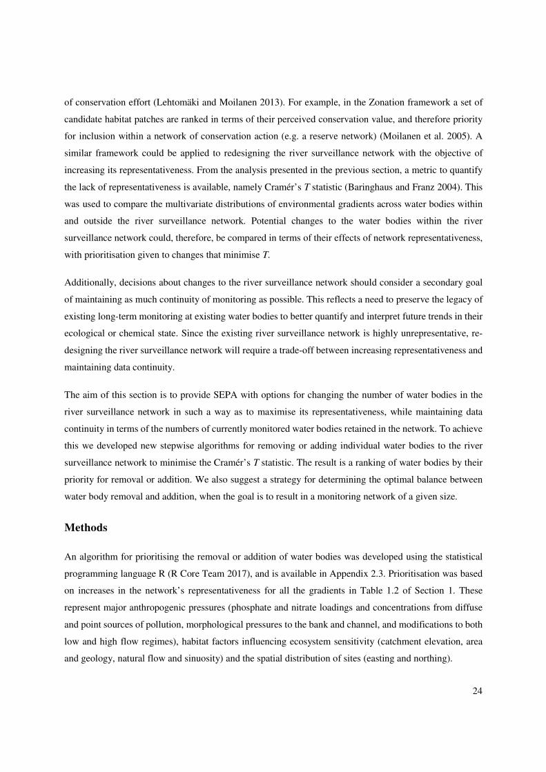
Figure 2.3. Effect of modifying the river surveillance network by reducing the number of water bodies to
100 and then adding 50 water bodies to maximise representativeness. Panels show cumulative distributions
of the gradients under consideration across all water bodies in Scotland (red), the existing river surveillance
network (green) and the reduced network (blue). As such the x-axes represent the values of the gradients
(see Table 1.2 for explanation and units) and the y-axes show the proportion of water bodies with values
less than or equal to the x-axis value. To enhance visualisation, upper extreme values beyond the 97.5th
percentile were excluded from the plots.
30
Discussion and conclusions
The stepwise algorithm developed for the prioritisation of water body removal and addition demonstrated
the scope for changing which river water bodies are monitored in the river surveillance network to achieve
a more representative coverage of key national pressure and environmental gradients. However, the analysis
also showed that achieving a statistically representative sample of Scotland’s water bodies would require a
combination of water body removal and addition, unless resources are so constrained that only 58 or fewer
water bodies can be maintained. Given this, SEPA will need to decide on the balance between water body
retention and water body addition in determining the new structure of the river surveillance network.
Retaining fewer water bodies from the existing river surveillance network will result in a more
representative network, but at the cost of lower long-term data continuity. Therefore, SEPA will need to
decide on the balance in importance between these two factors. Our recommendation would be to first
decide on the number of sites that can be supported in the network, given the current budget, and then
calculate the maximum number of currently-monitored water bodies that can be retained and the minimum
number of new water bodies that needs to be added to result in a statistically representative network (T <
5.10 indicating P > 0.05) of the desired size. For example, if only 125 water bodies can be monitored,
Figure 2.1 indicates that the way to achieve T < 5.10 while maximising existing river surveillance network
water body retention is to first reduce the existing river surveillance network to 100 water bodies and then
add 25 new water bodies.
The analysis here only considered network representativeness and data continuity in terms of retention of
currently monitored water bodies as a criteria to evaluate modifications to the river surveillance network.
We did not consider factors such as how long each currently-monitored site has been monitored for, or
whether candidate sites for addition to the network have been subject to existing monitoring for Operational
or Investigative purposes. Other factors important in determining optimal network structure, such as the
spatial balance of the network and logistical or access considerations, were also not taken account of. In
principal, the exercise here could be extended to include factors such as the history of monitoring and cost
of sampling each water body and the minimum travel time from SEPA offices. Doing this was beyond the
current project scope, but would be sensible for future investigation in making the final decision on how to
redesign the river surveillance network.
This analysis provides SEPA with options for increasing the representativeness of the river surveillance
network by altering its composition. However, the impact of such changes on the ability of the network to
detect long-term changes in ecological and chemical state caused by effects of multiple, potentially

31
interacting stressors remains unclear. Our expectation is that for a given network size, its efficiency will be
increased by taking a more representative sample of Scotland’s water bodies. To test this, power analysis
of trend-detection models on differently configured monitoring networks will be performed in Section 3.

32
3. Power of the river and loch sentinel networks to detect change
Summary
1. Power analysis was used to evaluate the ability of the current river and loch surveillance networks to
detect trends over time at the scale of the entire monitoring network, and to evaluate how modified
sampling strategies for the river surveillance network may influence the power to detect trends. Power
analysis for modified sampling regimes in the lochs network was outside the scope the study. The
results relate only to the power to detect trends. Other potential evidence needs from surveillance
networks, including classifying overall status and trends at individual water bodies, were not
considered.
2. The results indicate that the existing surveillance networks are generally less powerful than is desirable.
Using a benchmark of 80% power to detect a 5% change over ten years, only one out of the seven
monitored parameters achieved this in the river surveillance network (i.e. the invertebrate ASPT EQR)
and only one out of ten of the monitored parameters in the loch surveillance network (i.e. the diatom
LTDI2 EQR).
3. The power analysis of modified sampling regimes for the river surveillance network considered a range
of scenarios: the number of water bodies in the network, the interval between sampling years and the
number of samples per year during sampling years. The best way to maximise power for any given
level of resourcing was to avoid repeat sampling of water bodies in the same year. This is because it
allows sampling of a greater number of sites in a greater number of years, which means the data
averages out the spatial and annual variation obscuring the trend more efficiently.
4. The analysis also showed that reduced resourcing of the river surveillance network was incompatible
with boosting its power to detect trends in all monitored parameters at the benchmark level of 80%
power for a 5% change over ten years. However, it did highlight parameters for which the current (low)
power can be maintained at lower levels of resourcing, indicating that efficiency savings to the current
monitoring programme are possible.
5. Some sampling regimes with low to moderate levels of resourcing did not yield sufficient information
to robustly characterise trends over a ten-year period. These included monitoring water bodies very
rarely (e.g. one in six years with only one sample per sampling year) so that there was insufficient
replication at water body level in a ten-year period. Additionally, networks with very small numbers of
water bodies (i.e. 50), selected to be more representative of Scotland than the current network,
performed poorly. This was because very small representative networks did not include the full range

33
of rare water body typologies found across Scotland, allowing network trends to be skewed by trends
in the more common typologies.
6. Overall, this research shows that power analysis is a very valuable approach to design and revise
environmental monitoring programmes, and provides SEPA with recommendations for modifying its
surveillance networks for rivers and lochs to improve or maintain their ability to detect change at the
level of the whole network.
7. R code for running the power analysis can be found in Appendix 3.1 of this report.
Introduction and aims
The purpose of long-term environmental monitoring programmes is to produce reliable evidence about the
monitored ecological indicators or quantities. This can comprise information on the state of the
environment, environmental changes and ecological responses to change (Lovett et al. 2007; Lindenmayer
and Likens 2010). Crucially, whether or not a monitoring programme delivers this evidence satisfactorily
depends on the way sampling is conducted (Irvine et al. 2012). Therefore, it is important to consider how
the design of monitoring programmes influences the quality of evidence that can be delivered, and whether
this can be improved.
Evaluation of monitoring programme performance is generally done within the framework of power
analysis, which is an attempt to quantify the probability of rejecting an untrue null hypothesis, that is
detecting a true effect, using a particular statistical model and data structure (Cohen 1988). This approach
is especially valuable when existing monitoring programmes are being revised or redesigned, as is currently
the case for SEPA’s surveillance monitoring networks. For example, Irvine et al. (2012) conducted power
analysis of trends in water quality monitoring in Greater Yellowstone, USA. This allowed for evaluation of
the impact of choice of length of the monitoring programme, sampling frequency and sampling locations
on power to detect trends of different magnitude, while accounting for confounding factors such as
seasonality.
Given limited resourcing, SEPA must make decisions about which locations should be monitored and how
often should they be sampled, both in terms of annual sampling frequencies and how many samples are
collected during sampling years. To understand how these decisions are likely to influence evidence from
the monitoring network, recent monitoring data can be used to quantify the factors influencing power.
Essentially, this boils down to quantifying the relative strength of the signal and the noise in the monitoring
data, and how that noise is structured. The noise in environmental monitoring data arises from factors such
as seasonality, variation among sampling locations, variation among years, and unexplained sample-level

34
variation through measurement imprecision. Analyses of recent monitoring data can be used to quantify the
structuring of noise by such factors. Then, this information can be used in power analysis to estimate the
performance of ongoing monitoring under alternative sampling designs and data scenarios, assuming that
future noise will be similarly structured (Irvine et al. 2012, Johnson et al. 2015).
The scope of this chapter was restricted to the power of SEPA’s river and loch surveillance networks to
detect changes in terms of statistically significant trends over time in monitored parameters, at the scale of
the entire monitoring network. Therefore, all results and conclusions presented here preclude other potential
goals of monitoring networks, including assessing the current state across the whole network, attributing
changes to particular pressures, or characterising changes at individual monitoring locations. The specific
aims of the research were:
1. To estimate the minimum detectable trends in recent data from SEPA’s river and loch surveillance
networks.
2. To evaluate how altered monitoring strategies could change the power of the river surveillance network
to detect trends.
Methods
Overview
The first step in the power analysis was to fit models for trends in the monitoring data over a recent ten-
year period. These estimated the strength of the recent trend and characterised the structure of the noise
obscuring the trend. This noise was modelled as arising through seasonality, variation among water bodies
and types of water body, variation among years and other unexplained (residual) sample-level variance.
Based on these models, power analysis simulation techniques (Johnson et al. 2015) were used to estimate
the minimum detectable trends in the recent monitoring data from the river and loch networks, and also to
estimate the effect of modified monitoring network structures and sampling regimes on power to detect
trends in the river network.
Trend models
The power analysis was based on linear mixed effects (LME) models fitted to data from the surveillance
monitoring networks for rivers and lochs from 2007-2016, as provided by SEPA (Table 3.1). LMEs provide
a suitable analytical framework for monitoring data because of their ability to accommodate multiple levels
of variation as ‘random effects’ as well as trends of interest as ‘fixed effects’ (Bolker et al. 2009).

35
Separate LME models were fitted to each monitored parameter, as described in Table 3.1. Fixed effects
were specified for:
1. Year, to model the annual trend of interest. To aid model-fitting, year values were centred on their
midpoint.
2. Day of year, to account for seasonality in the monitored parameters. To model seasonality with a
flexible periodic function, linear terms were fitted for the first two harmonics of the Fourier series for
day of year, centred on zero and scaled to the same variance as the year variable, that is:
ℎ� = �� − 12 cos �2$�365 ℎ� = �� − 12 sin �2$�365 ℎ( = �� − 12 cos �4$�365 ℎ* = �� − 12 sin �4$�365
where Y=10 is the number of years of data and d is the day of year of the sample. Seasonal terms were
not included in models for macrophytes since these were sampled once per year and sampling dates
were not supplied.
Random effects were specified as:
1. Random intercepts for year, to model annual divergence from the overall trend.
2. Random intercepts for Water Framework Directive (WFD) river or loch typology, since similar types
of water body might have similar monitoring parameters. Typologies were defined based on all
permutations of the factors in Table 3.2.
3. Random intercepts for water body, nested within typology.
4. Where possible, random slopes for the annual trend were also specified for WFD typologies and water
bodies, nested within typology. This was only possible for models for the river network data, as the
lochs network contained too few water bodies for this. It was also not possible to include random trends
for river macrophytes, as there was insufficient data.
Prior to model fitting, response variables were transformed to meet model assumptions about the
distribution of residuals. For the chemistry parameters, logarithmic transformation was applied, to exclude
negative model predictions. Logarithmic transformations were also used for the ecological quality ratios
(EQRs) when supplied as precise values. However, when EQRs were supplied as ‘capped’ values with an

36
upper bound of 1, empirical logit transformations was applied as this is the preferred approach to model
proportion data (Warton and Hui 2011). The equation for the empirical logit transform of a proportion x is:
+∗ = ln � + + .1 − + + .
where ϵ is a small constant to avoid errors when x = 0 or x = 1. The value of ϵ was set at (1-xmax)/2, where
xmax is the largest value of x that is less than 1.
The LME models were developed using the R packages lme4 (Bates et al. 2015) and lmerTest (Kuznetsova
et al. 2015). Model fitting used restricted maximum likelihood (REML) and fixed effect statistical
significance was estimated using Satterthwaite’s approximation of the numbers of degrees of freedom.

37
Table 3.1. Monitored parameters for which power analysis was performed, a summary of their recent monitoring intensity and transformations used
in their analysis. The monitoring parameters were supplied by SEPA at the level of an individual sample. For classification purposes, SEPA
aggregates most of the parameters over longer time-periods.
Water
body
type
Monitoring
type
Monitored parameter Number
of
samples
(2007-
2016)
Number
of water
bodies
(2007-
2016)
Typical annual
sampling
frequency
(post- 2010)
Median
number of
samples per
year, when
sampled (post-
2010)
Transformation
for analysis
River Chemistry Ammonia as nitrogen (mg/L) 23510 246 every year 12 log10
Dissolved oxygen (mg/L) 22807 245 every year 11 log10
Total reactive phosphorus (mg/L) 23477 246 every year 12 log10
Total phosphorus (mg/L) 22695 246 every year 11 log10
Ecology Invertebrate EQR (Average Score Per Taxon, ASPT abundance) 3202 252 1 in 2 years 3 log10
Macrophyte EQR (River Macrophyte Nutrient Index, RMNI) 488 256 1 in 6 years 1 empirical logit
Diatom EQR (River Trophic Diatom Index, TDI4) 3662 252 2 in 3 years
(mix of 1 in 3
and 2 in 3)
2 empirical logit
Loch Chemistry Ammonia as nitrogen (mg/L) 4317 39 every year 12 log10
Dissolved oxygen (mg/L) 4265 39 every year 11 log10
Total reactive phosphorus (mg/L) 4182 39 every year 11 log10
Total phosphorus (mg/L) 4146 39 every year 11 log10
Ecology Invertebrates (ASPT abundance) 249 40 1 in 6 years 2 Scores from 0 to
8, so divided by
8 then logit
Invertebrates EQR (Chironomid Pupal Exuviae Technique, CPET) 267 40 1 in 6 years 4 empirical logit
Macrophyte EQR (Lake Macrophyte Nutrient Index, LMNI) 83 42 1 in 6 years 1 empirical logit
Diatom EQR (Lake Trophic Diatom Index, LTDI2) 493 40 1 in 2 years 2 empirical logit
Phytoplankton EQR (Phytoplankton trophic index, PTI)* 868 81 1 in 2 years 3 log10
Cyanobacteria EQR (PLUTO EQR)* 820 81 1 in 2 years 3 log10
* Data missing for 2007 and 2008

38
Table 3.2 Characteristics used to define water body typologies for rivers and lochs. These are based on the
Water Framework Directive definitions, as applied in the UK. However, loch size was not used because all
monitored lochs were in the ‘large’ category.
Rivers Lochs
Mean catchment altitude Low: < 200 m
Mid: 200-800 m
High: >800m
Mean altitude Low: < 200 m
Mid: 200-800 m
High: >800m
Catchment area Small: <100 km2
Medium: 100-1000 km2
Large: > 1000 km2
Dominant geology Siliceous
Calcareous
Organic
Catchment dominant
geology
Siliceous
Calcareous
Organic
Depth Shallow: < 3m
Deep: > 3m
Minimum detectable trends in the current monitoring data
To estimate the minimum detectable trend for each monitored parameter over the past ten years (2007-
2016), a power analysis was conducted on LMEs for the existing data using a range of annual trend values.
R code for running the power analysis can be found in Appendix 3.1. The procedure for the power analysis
followed recently-developed protocols (Johnson et al. 2015) and was as follows:
1. Decide a value of the annual trend to assess the power of the model. In this analysis, trend values
between 0 and values greatly exceeding the observed trends from 2007-2016 were tested. The
maximum trend values for each monitored parameter were chosen in a pilot study to ensure the analysis
included values with very high statistical power.
2. Simulate a large number of randomly generated response variables from the model, using the specified
value of the annual trend. For each assessment, 500 simulations were performed using the
‘simulate.merMod’ function of the lme4 R library (Bates et al. 2015). Simulations used:
a. The data used to fit the model. This defined the sampling regime in terms of the dates at which
each water body was sampled.
b. The specified value of the trend being tested.
c. Other fixed effects of the model (that is intercept and seasonality) at their fitted values.
d. Random effect variances and covariances, from which new multivariate normally-distributed
random effect values are generated at each simulation.

39
e. Residual (unexplained) variance from the model, from which normally-distributed errors are
included in the stochastic simulation.
3. Fit the same LME model to each simulated response variable and estimate the statistical power, which
is the proportion of simulations yielding a statistically significant annual trend.
The above procedure established a ‘power curve’, that is power to detect a significant trend as a function
of trend size (Johnson et al. 2015). The minimum detectable trend was estimated using linear interpolation
between points on the power curve to calculate the trend size where the power curve crossed 80% power
(that is a Type II error rate of 20%). This is a commonly used value for minimum adequate power, though
one that has been criticised (Di Stefano 2003).
Trend sizes here were obtained in terms of LME slope coefficients. For interpretation, they were converted
into the proportion change over a ten-year period using the following expressions:
1001�2�3 ifthevariablewaslog�?transformed10B�0C�2�� D − 110B20C�2�� D − 1 ifthevariablewaslog�?1+ + 13transformed
E11 + .3FB�0C�2�� D − .1 + FB�0C�2�� D GE 1 + FB20C�2�� D
11 + .3FB20C�2�� D − .G ifthevariablewasempiricallogittransformed
where a is the LME intercept, b is the LME slope for year, Y=10 is the number of years and ϵ is the empirical
logit offset. Note that these expressions are derived based on year values being centred on their midpoint
(that is 1� − 1 2⁄ 3). Coefficients for other fixed and random effects are not needed since the other fixed
effects were centred on zero and the random effects were modelled with zero mean.
Power of modified sampling regimes to detect trends in the river surveillance network
For the river surveillance network, power analysis experiments were performed to investigate how modified
network structures and altered sampling regimes may influence the ability of the model to detect trends
over a ten-year period (see Table 3.3). For this, the power analysis procedure described above was repeated
with two modifications:

40
1. The trend value was fixed at either the estimated trend from 2006-2017, or set to a value leading to
±5% change over ten years. The former was used to consider realistic trend values consistent with
recent data. The latter was chosen as a ‘target’ for good performance by the network. To implement
this, values of the trend leading to +5 and -5% changes differ slightly from one another, so both were
used and the results averaged.
2. In data simulations, instead of defining the sampling regime by inputting the historical monitoring data,
new sampling regimes were created and entered into the model. The modified sampling regimes
consisted of choices about which water bodies to include in the network and when to sample them, as
summarised in Table 3.3.
Table 3.3. Settings for the power analysis experiment. All factorial combinations of the treatment levels
were evaluated with 500 replicate simulations each.
Sampling regime feature Treatment levels
Trend in the monitored data Fixed at recent trend, or set to a value giving +/- 5% change over 10
years
Selection strategy for water bodies in the
network
Random subsets of the current water bodies or a more representative
set of water bodies
Number of water bodies in the network 50, 100, 150, 200 and either all current water bodies (for the random
selection) or 250 (for the representative selection)
Annual sampling interval 1, 2, 3, or 6 years
Number of samples per year 1, 6, or 12 for chemistry parameters; 1, 2 or 3 for ecology
parameters*
* except macrophytes, which are monitored with only 1 sample per year.
In the simulated sampling regimes, effort was distributed evenly across and within years. For example, if
sampling employed a 1 in 3-year rotation, then one third of the water bodies would be visited in each year.
Likewise, if sampling were done two times per year, then sampling dates for each water body would be
drawn randomly from the distribution of sampling dates in the 2007-2016 data, with one from the first half
of the year and one from the second half of the year.
To determine more representative subsets of water bodies to include, we used the results from Section 2 to
identify the stepwise strategy resulting in a statistically representative network (Cramér test with P > 0.05)
with the smallest loss of currently monitored water bodies. These were:
1. To select 50 water bodies – a stepwise reduction from the current network to 50 water bodies.

41
2. To select 100 water bodies – a stepwise reduction from the current network to 50 water bodies and then
a stepwise addition of 50.
3. To select 150 water bodies – a stepwise reduction from the current network to 100 water bodies and
then a stepwise addition of 50.
4. To select 200 water bodies – a stepwise reduction from the current network to 100 water bodies and
then a stepwise addition of 100.
5. To select 250 water bodies – a stepwise reduction from the current network to 150 water bodies and
then a stepwise addition of 100.
Some of the treatment combinations in the experiment resulted in simulated data sets to which the models
could not then be fitted. For the calculation of power, these were considered to yield non-significant trends,
since they represent sampling schemes not providing sufficient information to fit an appropriate trend
model.
Results
Trend models
The fitted models on which power analysis was performed are summarised in Table 3.4. From the river
surveillance network, the analysis indicated a statistically significant decrease in total reactive phosphorus
concentrations and significant improvements in the invertebrate and diatom EQRs. In the loch surveillance
network, there was a statistically significant increase in ammonia, a significant decrease in total phosphorus
and increases in the phytoplankton, cyanobacteria and invertebrate (CPET) EQRs.
Generally, the model fixed effects explained only a small amount of the variation compared to the random
effects or residual unexplained variation. Across all monitoring parameters, the marginal R2 (from fixed
effects only) had a median value of 0.015 in rivers and 0.021 in lochs, while median values of the
conditional R2 (from fixed and random effects) were 0.660 in rivers and 0.477 in lochs. Therefore, in
general, less than 2.1% of the variation in the data was explained by the annual trend (since marginal R2
combined effects of the annual trend as well as seasonality). Examination of the random effects (Table 3.4)
suggests that spatial (among water body) variability was greater than year-to-year variations, and that there
was more variability among water bodies within a typology than between typologies.

42
Minimum detectable trends in the current monitoring data
Power curves from the analyses of the river and loch surveillance networks are shown in Figures 3.1 and
3.2. From these, the minimum detectable trends were estimated as the trend size yielding 80% power
(Figure 3.3). Generally, the power for the observed trends was below 80%, meaning that observed trends
from 2007-2016 were weaker than the minimum detectable trends. The sole exception to this was river
invertebrates (ASPT EQR), for which the current significant trend was estimated to have 85% power.
Only two parameters had minimum detectable trends less than ±5% over ten years, seen as a ‘target’ for
good network performance by SEPA. These were for river invertebrates (ASPT EQR) and loch diatoms
(LTDI2 EQR). By contrast, minimum detectable trends greater than ±10% were observed in the river
surveillance network for total reactive phosphorus, ammonia as nitrogen and total phosphorus, and in the
loch surveillance network for ammonia as nitrogen, total reactive phosphorus , total phosphorus, EQRs for
macrophytes, cyanobacteria and phytoplankton and invertebrates (ASPT). These can be considered the
parameters for which the network seems to have performed most poorly.

43
Table 3.4. Summary of the LME models for which power analyses were performed. The table shows the estimated annual trends (in bold where P
< 0.05), an indication of whether the model found significant seasonality and the random effect and residual standard deviations. All results are on
the scale of the transformed monitoring parameters.
Water
body
type
Monitoring
type
Monitored parameter Annual trend on
transformed scale
(SE)
P Significant
seasonality
Random intercepts and residuals
(standard deviations)
Random slopes for year
(standard deviations)
River Chemistry Ammonia as nitrogen 6.87x10⁻³ (4.67x10⁻³) 0.160 yes Year: 0.027
Typology: 0.236 Typology: 0.0102
WB within
typology:
0.268 WB within
typology:
0.0282
Residual: 0.306
River Chemistry Dissolved oxygen 2.83x10⁻⁴ (9.02x10⁻⁴) 0.761 yes Year: 0.00793
Typology: 0.00497 Typology: 0.0006065
WB within
typology:
0.01495 WB within
typology:
0.0015582
Residual: 0.03369
River Chemistry Total reactive phosphorus -1.42x10⁻³ (5.71x10⁻⁴) 0.027 yes Year: 0.00447
Typology: 0.01688 Typology: 0.0007276
WB within
typology:
0.0269 WB within
typology:
0.0024204
Residual: 0.03043
River
Chemistry Total phosphorus -5.90x10⁻³ (3.29x10⁻³) 0.099 yes Year: 0.02625
Typology: 0.29274 Typology: 0.003195
WB within
typology:
0.29815 WB within
typology:
0.015847
Residual: 0.2305

44
Water
body
type
Monitoring
type
Monitored parameter Annual trend on
transformed scale
(SE)
P Significant
seasonality
Random intercepts and residuals
(standard deviations)
Random slopes for year
(standard deviations)
River Ecology Invertebrate EQR 1.06x10⁻³ (3.22x10⁻⁴) 0.010 yes Year: 0.00193
Typology: 0.01373 Typology: 0.0004635
WB within
typology:
0.02594 WB within
typology:
0.0019569
Residual: 0.02176
River Ecology Macrophyte EQR 0.0565 (0.021) 0.074 - Year: 0.117
Typology: 1.139
WB within
typology:
0.859
Residual: 1.035
River Ecology Diatom EQR 0.0383 (0.0132) 0.022 yes Year: 0.042
Typology: 0.446 Typology: 0.0275
WB within
typology:
1.023 WB within
typology:
0.0717
Residual: 1.202
Loch Chemistry Ammonia as nitrogen 0.0174 (7.06x10⁻³) 0.040 yes Year: 0.06248
Typology: 0.12065
WB within
typology:
0.16596
Residual: 0.3012
Loch
Chemistry Dissolved oxygen 4.82x10⁻⁴ (8.89x10⁻⁴) 0.603 yes Year: 0.0079
Typology: 0
WB within
typology:
0.00956
Residual: 0.03515

45
Water
body
type
Monitoring
type
Monitored parameter Annual trend on
transformed scale
(SE)
P Significant
seasonality
Random intercepts and residuals
(standard deviations)
Random slopes for year
(standard deviations)
Loch Chemistry Total reactive phosphorus -1.42x10⁻³ (4.43x10⁻³) 0.757 yes Year: 0.03858
Typology: 0.06682
WB within
typology:
0.1446
Residual: 0.23276
Loch Chemistry Total phosphorus -3.71x10⁻³ (1.55x10⁻³) 0.045 yes Year: 0.0102
Typology: 0.2052
WB within
typology:
0.2612
Residual: 0.2002
Loch Ecology Invertebrates ASPT EQR -4.86x10⁻⁴ (0.0130) 0.972 no Year: 0.0673
Typology: 0.2672
WB within
typology:
0.3696
Residual: 0.4474
Loch Ecology Invertebrates CPET EQR 0.0397 (0.0176) 0.025 no Year: 0
Typology: 0.2405
WB within
typology:
0.5984
Residual: 0.7069
Loch
Ecology Macrophyte EQR 0.0411 (0.0247) 0.170
Year: 0.07733
Typology: 0.11644
WB within
typology:
0.51632
Residual: 0.58057

46
Water
body
type
Monitoring
type
Monitored parameter Annual trend on
transformed scale
(SE)
P Significant
seasonality
Random intercepts and residuals
(standard deviations)
Random slopes for year
(standard deviations)
Loch Ecology Diatom EQR 3.52x10⁻³ (0.0321) 0.913 yes Year: 0
Typology: 0
WB within
typology:
1.699
Residual: 1.811
Loch Ecology Phytoplankton EQR 5.24x10⁻³ (1.73x10⁻³) 0.003 yes Year: 0
Typology: 0.07445
WB within
typology:
0.12854
Residual: 0.10757
Loch Ecology Cyanobacteria EQR 4.09x10⁻³ (1.58x10⁻³) 0.041 no Year: 0.00921
Typology: 0.0096
WB within
typology:
0.0208
Residual: 0.0422
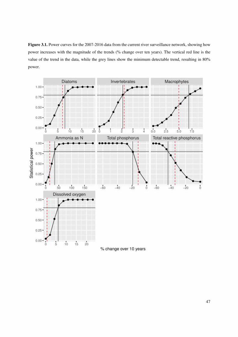
47
Figure 3.1. Power curves for the 2007-2016 data from the current river surveillance network, showing how
power increases with the magnitude of the trends (% change over ten years). The vertical red line is the
value of the trend in the data, while the grey lines show the minimum detectable trend, resulting in 80%
power.
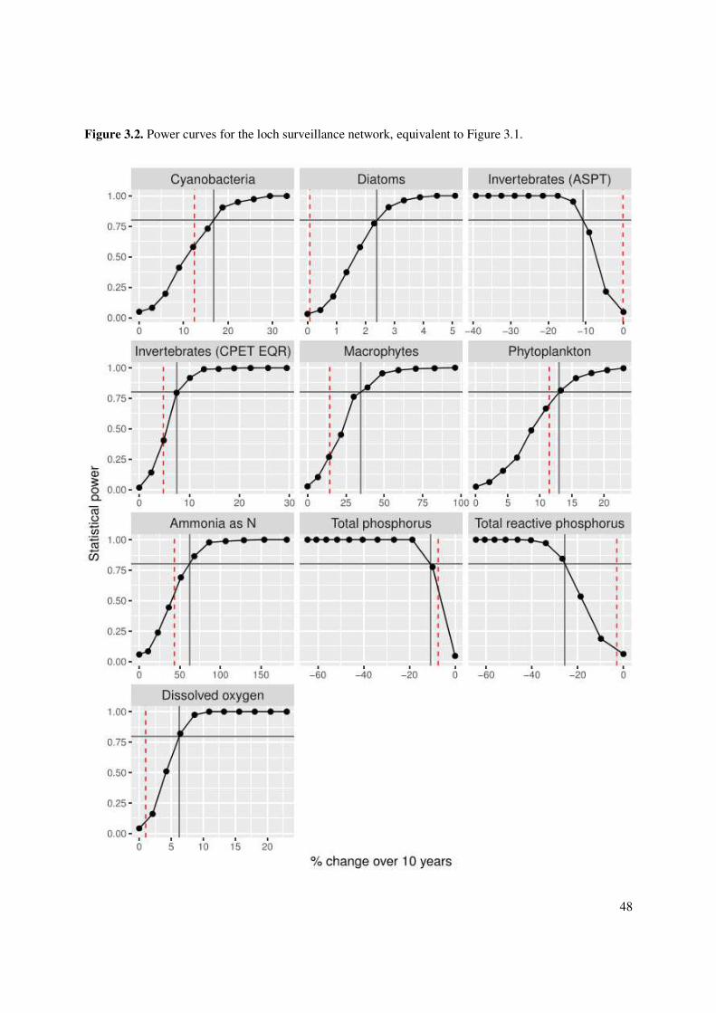
48
Figure 3.2. Power curves for the loch surveillance network, equivalent to Figure 3.1.

49
Figure 3.3 Observed and minimum detectable (80% power) trends in the 2007-2016 monitoring data from
(a) rivers and (b) lochs. Dashed lines show ±5%, considered an upper limit for the minimum detectable
trends in a monitoring network.
(a)
(b)
Power of modified sampling regimes to detect trends in the river surveillance network
Power experiments with simulated data from modified sampling regimes were performed assuming a ten-
year period with both the estimated 2007-2016 trends (Figure 3.4) and with trend values resulting in an
overall change of ±5% in each parameter (Figure 3.5). In both cases, an increase in the number of samples
collected generally resulted in higher power. However, there appeared to be some scope to reduce the
number of samples with minimal power loss. Furthermore, the best way to reduce resourcing, while
maintaining the network’s ability to detect trends, is to reduce repeat sampling within years while
maintaining as many sites as possible and sampling them in as many years as possible. For any given level
of resourcing, the highest power was obtained with the lowest level of repeat sampling within years
considered in the experiment.

50
The plots also identify two clusters of points with distinctly low power, representing sampling regimes that
should be avoided. First, there was a cluster of sampling regimes at zero power. These were sampling
regimes with monitoring in one in six years and only one sample per year. Such schemes yielded data that
did not allow the trend model to be fitted because there was insufficient replication at water body level to
estimate variation among water bodies as well as seasonality and year effects. In addition, there was a group
of sampling regimes yielding low power from the more representative networks. These were representative
networks of only 50 water bodies, the smallest network sizes considered. It is likely that this resulted from
the small representative networks not including the rarer river typologies, and, therefore, having a high
chance of the trends being obscured by among-typology variation in a small number of common typologies.
For larger networks, however, there was little effect of representativeness on network performance at trend
detection, although it is to be expected that the representative networks would yield more representative
trend estimates.

51
Figure. 3.4 The estimated power of modified river surveillance sampling regimes to detect the recent (2007-
2016) trends over a ten-year period. Statistical power is plotted as a function of total resourcing per
parameter (number of samples taken over ten years). The point shapes and shading indicate the effects of
choice of water body selection strategy and within-year sampling intensity, as these appeared to be the two
key factors affecting power, in addition to the number of samples. The grey lines indicates the number of
samples taken from 2007-2016.

52
Figure. 3.5 The estimated power of modified river surveillance sampling regimes to detect a trend of ±5%
change over a ten-year period. The plot is otherwise equivalent to Figure 3.4.

53
Discussion and conclusions
This research was motivated by SEPA’s need to operate a freshwater surveillance network that delivers
high quality evidence in the most cost-effective manner. We used power analysis to evaluate the ability of
the river and loch monitoring networks to detect trends over a ten-year period. Therefore, all our results and
recommendations should be interpreted in the context of trend detection ability at the level of the whole
network, and may not apply to other evidence needs from the surveillance monitoring networks, such as
managing the condition of individual river or loch water bodies.
The power analysis indicated that the current river and loch surveillance networks did not achieve sufficient
power for detecting trends of the observed magnitude. Trends in monitoring data from 2007-2016 were
generally below the estimated minimum detectable trends for each parameter, defined as the trend value
giving 80% power. This would not necessarily be interpreted as a problem, since it may be that the
monitored parameters were not exhibiting strong trends. Of more concern, however, is that these minimum
detectable trends were often large. For example, we found <80% power to detect changes of more than
±5% over a ten-year period in six out of seven monitored parameters in rivers and nine out of ten monitored
parameters in lochs. The two exceptions were trends for river invertebrates (ASPT EQR) and loch diatoms
(LTDI2 EQR), where the minimum detectable trends were <±5%, even though no actual trend was detected
for diatoms.
This variation among monitoring parameters in both recent trends and the minimum detectable trends,
suggests current sampling effort is not distributed optimally across parameters. Potentially, it would be
desirable to shift effort from parameters with a small minimum detectable trend to those with a high one,
in order to equalise the minimum detectable percentage change across parameters. For example, Ammonia
as nitrogen and total reactive phosphorus would benefit from improved monitoring to bring down their
large minimum detectable trends in both rivers and lochs.
The power analysis also considered modified sampling regimes for the river surveillance network, informed
by SEPA’s need to modify their current surveillance monitoring. This demonstrated the value of power
analysis for re-designing monitoring networks and sampling regimes (Irvine et al. 2012). In particular, it
showed that for a given level of resourcing, power was maximised by moving towards sampling only once
per year. This likely reflects an ability of the statistical models to characterise seasonality across water
bodies, and remove its influence on apparent trends without a need to intensively sample across the year in
all monitored water bodies. Sampling only once per year also means resources can be spread more widely

54
across a range of water bodies and typologies, so the model averages out spatial and between-typology
variability more effectively and produces a more accurate estimate of the average trend.
It should be noted however, that while this improves power for detecting trends at the level of the whole
network, it may not deliver sufficient information on the status or trends of individual water bodies or
typologies. This includes WFD classification for the condition of individual water bodies. Consideration of
these goals were outside the scope of the analysis performed here, but should be undertaken by SEPA when
making decisions on how to adjust their surveillance networks. This could be done using similar power
analysis approaches to the one we developed here.
The power analysis on modified sampling regimes also highlighted the need for clearly defined goals and
targets for trend detection by the modified network. Below, the results are evaluated in terms of three
alternative goals for a modified river surveillance network:
1. If the goal is to maintain current power to detect trends of similar magnitude to those of the past ten
years, then Figure 3.4 suggests that substantial reductions in sampling of chemical determinands can
be made without substantial loss of their current (low) power. By contrast, reduced sampling effort for
the ecological parameters results in greater power loss, suggesting their sampling should be maintained
or intensified.
2. If the goal is to maintain current power to detect trends of ±5% over ten years, then Figure 3.5 suggests
reduced sampling of invertebrates, as well as chemistry. This is because the current network has
relatively high power for river invertebrate trends, with a minimum detectable trend of ~2%. Therefore,
invertebrate sampling intensity can be reduced to the point where the minimum detectable trend is ±5%.
3. If the goal is to achieve a minimum adequate level of power across all monitored parameters, then the
level of resourcing will determine how much power can be achieved. For example, if the goal is to
achieve 80% power for a ±5% change in all parameters, then Figure 3.5 suggests this cannot generally
be done with current or reduced resourcing. However, since current sampling is more than adequate for
invertebrates, we would recommend redistributing some of the effort towards the parameters currently
having the lowest power to detect ±5% change (ammonia as nitrogen, total phosphorus and total
reactive phosphorus). Based on the arguments above, greater sampling of these parameters is likely to
be most effective at trend detection if achieved by adding new water bodies to the network and sampling
the expanded network only once per year. Although, the power experiment did not evaluate the potential
power gain under this scenario it seems likely that improvements on current power could be achieved
with similar or improved resourcing.

55
Power analysis is always approximate and subject to a number of caveats (Johnson et al. 2015). One caveat
comes from the assumption that the structure of noise in future monitoring data will follow patterns from
the last ten years. This may not be true because emerging technologies for monitoring may improve
accuracy (that is reduce sample-level residual variation), there may be better standardisation of sampling
and laboratory methods, or factors such as climate change may alter seasonality, among-water body,
among-typology and among-year variability. Another caveat is that assumptions of the trend model may
not have been fully met in the data. Nevertheless, the power analysis approaches developed and applied
here should be considered an important element in the design of environmental monitoring programmes. In
this context, our results provide SEPA with information to interpret evidence about trends from their
existing surveillance networks as well as suggest options for modifying their networks under different levels
of future resourcing.

56
4. Long-term changes detectable in the existing river and loch sentinel
networks
Summary
1. In this section, trends over time in the river and loch surveillance networks from 2007-2016 were
evaluated with both linear and nonlinear trend models.
2. Linear trend models for the river surveillance network detected upward trends in invertebrates and
diatoms and a decline in total reactive phosphorus. For the loch network, there were significant
increases in EQRs for invertebrates (CPET), phytoplankton and cyanobacteria, a reduction in total
phosphorus and an increase in ammonia. Since we previously found that the networks had relatively
low power to detect trends in most parameters, it is not surprising that more significant trends were not
found.
3. Trend variation among river water body typologies was present, but the patterns of variation were not
consistent across river typologies. This probably reflects both a relatively small number of water bodies
representing many of the individual typologies in the river surveillance network and a general finding
that there was more variation among water bodies within typologies than between typologies.
4. Many of the monitored parameters appeared to exhibit non-linear trends that fitted the data better than
the linear trend models. This was particularly evident for larger monitoring datasets, where the greater
amount of data allowed the use of more parameter-rich models, such as those were the trend is modelled
with a smoothing spline. These allow testing and visualisation of non-linear trends, but do not yield a
direct estimate of the form or magnitude of the trend. As such, they complement the use of the linear
models for analysis and interpretation of monitoring trends.
Introduction and aims
The identification of trends is one of the key goals of environmental monitoring programmes (Lindenmayer
and Likens 2010). It is especially important for so-called ‘mandated’ monitoring where the focus is on
determining whether the state of the environment is changing over time, rather than trying to attribute that
change to a particular cause. SEPA’s surveillance monitoring networks for rivers and lochs can be
considered to fall into this category, with operational and investigative monitoring designed to identify and
manage drivers of local change.

57
As demonstrated in the previous section, trend detection in noisy monitoring datasets requires large volumes
of data, ideally collected across many sites and over a long time-period. Therefore, after around ten years
of operation in their current form, there is an opportunity to evaluate long-term trends across both
surveillance networks for a range of ecological and chemical parameters. However, ability to detect trends
depends not only on the sampling regime and volume of data, but also on whether the chosen trend model
is appropriate for the type of trend present in the data. Specifically, linear trend models are commonly
applied but could perform poorly at detecting more complex nonlinear trends. Therefore, it is beneficial to
complement the linear models with application of more flexible nonlinear trend models.
In Section 3 we used linear trend models to perform power analysis aimed at evaluating the ability to detect
changes in current and modified surveillance networks for rivers and lochs. This section focuses on the
actual trends revealed in that analysis. The specific aims were:
3. To summarise the linear trends in the river and loch surveillance networks from 2007-2016, including
variation in trends among water body typologies, where possible.
4. To evaluate whether linear trends are an appropriate model for observed changes in the surveillance
network data, or whether nonlinear models are required.
Methods
Overview
Linear and nonlinear trend models were fitted to data from the river and loch surveillance monitoring
networks from the ten-year period 2007-2016. The data used in the modelling is fully described in Section
3. For the river network, trends were estimated for ammonia, dissolved oxygen, total reactive phosphorus,
total phosphorus, invertebrates (ASPT EQR), macrophytes (RMNI EQR) and diatoms (TDI4 EQR). For
the loch network, trends were estimated in ammonia, dissolved oxygen, total reactive phosphorus, total
phosphorus, invertebrates (CPET EQR and raw ASPT abundance), macrophytes (LMNI EQR), diatoms
(LTDI2 EQR), phytoplankton (PTI EQR) and cyanobacteria (PLUTO EQR).
Linear trend models
The trend models reported here are those fitted for the trend power analysis in Section 3. For full details of
the methods, see Section 3. In overview, linear mixed effects (LME) models were fitted in R package ‘lme4’
(Bates et al. 2015) to surveillance monitoring data for rivers and lochs from 2007-2016 as provided by
SEPA (see Table 3.1). Fixed effects were specified for the covariates year (the trend of interest) and
harmonics of the day of year (to model seasonality), except that seasonality could not be modelled for

58
macrophytes which are only sampled once per year. Random intercept effects were specified for year (to
model annual divergence from the overall trend), and water bodies nested within river or loch Water
Framework Directive (WFD) typology (see Table 3.2 for definitions). For models fitted to the river
surveillance network data, random slope effects for the year trend were also specified for water bodies
nested within typology, except in the analysis of macrophytes where there was insufficient data to do this.
To summarise these models here, the magnitude and statistical significance of the annual trends are
reported, as well as the estimated variation in trends among river typologies.
Nonlinear trend models
The above trend models were designed to detect a linear trend through the specification of a fixed effect of
year, centred on its midpoint. To examine whether there may have been pronounced deviation from a linear
trend, two approaches were used to visualise and characterise nonlinear trends.
First, LMEs were fitted with year as a fixed factor rather than linear covariate. The LME specification
included:
1. Fixed effect of year as a factor, rather than as a covariate and random effect.
2. Fixed terms for day of year, capturing seasonality and modelled using harmonics as described above.
3. Random intercepts for water body nested within typology, capturing site effects.
Note that the random year trends in the previous models are not specified since no trend is actually
estimated. To visualise departures from a linear trend, patterns in the fitted year coefficients were examined.
Second, we fitted generalised additive mixed models (GAMMs) to the data, using flexible smoothing
splines for the responses to year and day of year. The GAMM models were fitted in the R package ‘gamm4’
(Wood and Scheipl 2017) which estimates the appropriate flexibility in the spline responses supported by
the data. The spline degrees of freedom is therefore a measure of trend complexity and deviation from a
linear trend (one degree of freedom). The GAMM specification included:
1. Smoothing spline for year, centred on its midpoint and restricted to a maximum of 6 degrees of freedom
(since there were only a maximum of ten years of data).
2. Smoothing spline for day of year, centred on the year midpoint, to model seasonality.
3. Random intercepts for water body nested within typology, capturing site effects.

59
Results
Linear trend models
The annual trends estimated by LMEs for the monitoring networks from 2007-2016 are summarised in
Table 4.1 (see also Table 3.4 for full model details). For the river surveillance network, the LMEs identified
statistically significant increases in the EQRs for invertebrates and diatoms, and a significant decrease in
total reactive phosphorus. The increase in the macrophyte EQR and decrease in total phosphorus
concentrations almost achieved statistical significance and these are consistent with the significant trends
in the other ecological parameters and total reactive phosphorus. In the loch surveillance network, there
were significant increases in the phytoplankton, invertebrate (CPET) and cyanobacteria EQRs (Table 4.1).
These were accompanied by a significant increase in ammonia concentrations and a significant decrease in
total phosphorus concentrations.
Variation in trends among river typologies was modelled as a random slope effect in the LMEs for the river
surveillance network. The random effects are plotted as standardised trends in Figure 4.1. This gives little
indication that the analysed parameters had similar trends across typologies, even for related parameters
such as total phosphorus and total reactive phosphorus. An explanation for this may lie in the relatively
small numbers of water bodies representing each typology. Although generally adequate for LME
modelling, where a rule of thumb is to have more than five replicates of each random effect level (Bolker
et al. 2009), the relatively low site-level replication variation among typologies probably precludes
meaningful comparison of trends among typologies.
Nevertheless, there is a suggestion that catchment geology type may have influenced ecological trends. In
particular, the upward trend in invertebrates appeared strongest in typologies with calcareous geology
(Figure 4.1). Conversely, the upward trends in both diatoms and invertebrates appeared weaker than average
in siliceous typologies.

60
Table 4.1 Summary of long-term trends in the monitoring parameters in the river and loch surveillance
networks from 2006-2017. Annual trends are the fitted LME coefficients for year, showing annual change
in the monitoring parameters on their transformed scales and their standard errors (see Table 3.4 for full
details of the models). Statistically significant trends are displayed in bold. Trends have been converted
into equivalent expected changes over the ten-year period of the data, with 95% confidence intervals
calculated from the standard error of the trends.
Water
body
type
Monitoring
type
Monitored parameter Annual trend
on transformed
scale (SE)
P Equivalent % change
in 10 years (95% CI)
Rivers Chemistry Ammonia as nitrogen (mg/L) 6.87x10⁻³
(4.67x10⁻³)
0.160 +15.3 (-4.6 to +39.4)
Dissolved oxygen (mg/L) 2.83x10⁻⁴
(9.02x10⁻⁴)
0.761 +0.6 (-3.0 to 4.3)
Total reactive phosphorus (mg/L) -1.42x10⁻³
(5.71x10⁻⁴)
0.027 -34.6 (-54.3 to -6.4)
Total phosphorus (mg/L) -5.90x10⁻³
(3.29x10⁻³)
0.099 -11.5 (-22.6 to 1.1)
Ecology Invertebrate EQR (Average Score Per
Taxon, ASPT abundance)
1.06x10⁻³
(3.22x10⁻⁴)
0.010 +2.2 (+0.9 to +3.6)
Macrophyte EQR (River macrophyte
nutrient index, RMNI)
0.0565 (0.021) 0.074 +5.0 (+1.3 to +8.9)
Diatom EQR (River Trophic Diatom
Index, TDI4)
0.0383 (0.0132) 0.022 +7.0 (+2.2 to +12.0)
Lochs Chemistry Ammonia as nitrogen (mg/L) 0.0174
(7.06x10⁻³)
0.040 +43.3 (+7.6 to +90.9)
Dissolved oxygen (mg/L) 4.82x10⁻⁴
(8.89x10⁻⁴)
0.603 +1.0 (-2.6 to +4.7)
Total reactive phosphorus (mg/L) -1.42x10⁻³
(4.43x10⁻³)
0.757 -2.9 (-18.9 to 16.2)
Total phosphorus (mg/L) -3.71x10⁻³
(1.55x10⁻³)
0.045 -7.4 (-13.1 to -1.4)
Ecology Invertebrates (ASPT abundance) -4.86x10⁻⁴
(0.0130)
0.972 -0.1 (-6.0 to +6.1)
Invertebrates (CPET EQR) 0.0397 (0.0176) 0.025 +4.9 (+0.6 to +9.3)
Macrophyte EQR (Lake Macrophyte
Nutrient Index, LMNI)
0.0411 (0.0247) 0.170 +14.4 (-2.3 to +34.3)
Diatom EQR (Lake Trophic Diatom
Index, LTDI2)
3.52x10⁻³
(0.0321)
0.913 +0.1 (-1.3 to +1.5)
Phytoplankton EQR (Phytoplankton
trophic index, PTI)*
5.24x10⁻³
(1.73x10⁻³)
0.003 +11.5 (+3.9 to +19.6)
Cyanobacteria EQR (PLUTO EQR)* 4.09x10⁻³
(1.58x10⁻³)
0.041 +12.4 (+2.9 to +22.9)
* Data missing for 2007 and 2008

61
Figure 4.1 Visualisation of standardised variation in trends among typologies in the river surveillance
network. Typology labels reflect altitude (low or mid), catchment area (small, medium or large) and
geology type (siliceous, calcareous or organic) (see Table 3.2). Shading indicates the random year slopes
for each monitored parameter, standardised by dividing by the overall standard deviation for the typology
effect, multiplied by the sign of the trend. Large positive values indicate that trends were more extreme
than average (more positive or more negative), while large negative values indicate trends that were closer
to zero or even reversing the main trend direction. The number show the number of water bodies monitored
in each typology. Trend variation could not be estimated for macrophytes, which are shaded in grey.

62
Nonlinear trend models
When LMEs were fitted with year as a fixed factor, rather than a linear covariate and random effect,
ANOVA’s on the year effect found statistically significant year-to-year variability in most parameters
(Table 4.2). The exceptions to this were loch invertebrates (ASPT), loch diatoms and loch macrophytes.
Plots of the estimated year coefficients (Figures 4.2 and 4.3) show that some of the variation over years
could be well approximated with linear trends. For example, trends in river invertebrates, loch
phytoplankton and total phosphorus. However, many of the parameters exhibited strong fluctuations from
year-to year or apparent step changes in their trends (e.g. river macrophytes, loch ammonia), suggesting
more complex trend models may be required.
These impressions were borne out by the GAMM models, where the optimal splines for the year effect
tended to degrees of freedom greater than one. This indicates that a nonlinear trend tended to fit better than
a linear one (Table 4.2). The main exceptions to this pattern were ecological parameters in the loch network,
which mostly supported a linear trend model (d.f. = 1). The spline curves are not plotted here, as they follow
the form of Figures 4.2 and 4.3, with some smoothing of the year-to-year variation.

63
Table 4.2. Summary of the year effects in two types of nonlinear trend model for the river and loch
surveillance networks from 2007-2016. First, year was entered as a fixed factor in LME models and the
year effect tested by ANOVA with the Satterthwaite's approximation to the denominator degrees of freedom
(d.f., given as numerator, denominator). Second, GAMM models with smoothing splines for year were
fitted. The estimated d.f.s indicate spline complexity and, when greater than 1, deviation from a linear trend.
Water
body
type
Monitoring
type
Monitored parameter Year factor effect in LME Year effect in GAMM
ANOVA
F
d.f. P Spline
complexity
(d.f.)
P
Rivers Chemistry Ammonia as nitrogen 23.35 9, 23271 <0.001 4.765 <0.001
Dissolved oxygen 97.1 9, 22609 <0.001 4.896 <0.001
Total reactive phosphorus 230.20 9, 23231 <0.001 4.957 <0.001
Total phosphorus 37.56 9, 22447 <0.001 4.896 <0.001
Ecology Invertebrate EQR 10.1859 9, 2976.9 <0.001 2.750 <0.001
Macrophyte EQR 2.6121 9, 383.77 0.006 3.041 0.001
Diatom EQR 3.1228 9, 3420.6 <0.001 2.293 <0.001
Lochs Chemistry Ammonia as nitrogen 28.758 9, 4266.4 <0.001 4.764 <0.001
Dissolved oxygen 20.56 9, 4219.0 <0.001 3.589 <0.001
Total reactive phosphorus 11.133 9, 4131.1 <0.001 4.514 <0.001
Total phosphorus 3.179 9, 4094.3 <0.001 1.961 0.001
Ecology Invertebrates (ASPT abundance) 1.28309 9, 217.54 0.247 1.669 0.551
Invertebrates (CPET EQR) 0.85752 9, 236.14 0.5640 1 0.039
Macrophyte EQR 1.310 9, 54.327 0.2536 1 0.087
Diatom EQR 0.6924 9, 445.06 0.71597 1 0.838
Phytoplankton EQR 1.4480 7, 796.29 0.18277 1 0.002
Cyanobacteria EQR 9.6001 7, 694.24 <0.001 4.100 <0.001

64
Figure 4.2 Estimated annual variation in the monitored variables in the river surveillance network on their
transformed scales (LME coefficients ± 1 standard error), as estimated by LME models with year as a fixed
factor effect. The coefficients represent deviation in the mean transformed value from that in the first year
of the data.

65
Figure 4.3 Estimated annual variation in the monitored variables in the loch surveillance network on their
transformed scales (LME coefficients ± 1 standard error), as estimated by LME models with year as a fixed
factor effect. The coefficients represent deviation in the mean transformed value from that in the first year
of the data.

66
Discussion and conclusions
Linear trend models fitted to SEPA’s surveillance network detected a number of statistically significant
trends over time in a recent ten-year period. In the river network, there were upward trends in river
invertebrates and diatoms, and a decline in total reactive phosphorus. In the loch network, the models found
significant increases in EQRs for invertebrates (CPET), phytoplankton and cyanobacteria, accompanied by
a reduction in total phosphorus but an increase in ammonia. The lack of significant trends in other
parameters should be viewed in the context of the power analysis in Section 3, which found that the
networks had relatively low power to detect reasonable changes of ±5% in most parameters. Thus, it is not
surprising that all trends did not reach statistical significance. Nevertheless, the trends evident in the data
do suggest an improving state of Scotland’s freshwater environment, with the exception of the increase in
loch ammonia concentrations.
From the linear trend models of the river surveillance network, it was possible to examine between-typology
variation in trends, as estimated in the random effect structure. This did not reveal any clear mediation of
trends by typology across monitoring parameters, although there was some suggestion that ecological trends
may have been influenced by geology type. This lack of a clear consistent typology effect was probably
caused by the relatively low number of water bodies represented in the river network for many of the
typologies, especially since trend variation among water bodies within a typology was much larger than the
trend variation among typologies. For future analyses, it would be desirable to see whether alternative water
body groupings could provide a stronger structuring of trend variation. For example, if pressure gradients
drive the trends, but these are not tightly correlated to typologies, then using groupings based on pressures
(pressure typologies) may have been a better strategy. If so, this could also help in determining the ability
of surveillance monitoring to attribute ecological and chemical trends to particular pressures, although that
goal was beyond the scope of this study.
The analysis also supported the use of nonlinear trend models for analysis of long-term changes in the
surveillance networks. Both the LMEs with year as a fixed factor and the GAMMs where the trend was
modelled with a smoothing spline generally indicated significant changes over time following more
complex trends than were represented by the linear models. These nonlinear trend models are more
parameter-rich than the linear trend models, making them especially suitable for complex trends in larger
monitoring data sets. This was evidenced by their relatively poor performance for the ecological data from
the lochs network, which had the lowest sample sizes. As such, they would be especially suitable for even
longer time series of monitoring data, where departures from linear trends are likely to be even more
apparent. However, unlike the linear trend models, they do not provide a direct estimate of the type of trend

67
and so require visualisation for interpretation. This, along with the computational intensiveness of GAMMs,
will likely preclude their use in power analyses aimed at evaluating current monitoring or designing new
monitoring strategies. Therefore, we suggest linear and non-linear models should both be used for future
trend analyses.
The strongest estimated trends were for monitoring variable that required modelling on a logarithmic scale
and tended to be those that were estimated the least precisely (see Table 4.1). For example, the estimated
43% increase in loch ammonia had a 95% confidence interval of being an 8 to 91% increase, while the 35
% decrease in river total reactive phosphorus had a 95% confidence interval of being a 6% to 54% decrease.
Part of this uncertainty was because these trends were modelled on a log10-scale, meaning that uncertainty
in the fitted trend coefficient propagates exponentially into the estimates of percent changes. The large
uncertainty also resulted from these variables being among those for which the non-linear trend models
identified the strongest departures from linear trends. For example, loch ammonia decreased sharply from
2007 to 2010, then increased until 2014 before stabilising (Figure 4.3), a pattern also seen in the rivers
(Figure 4.2). River total reactive phosphorus increased in 2008 from 2007 levels, but then fell until 2013,
after which increases were apparent. Similar patterns were seen in river total phosphorus, though trends in
lochs appeared qualitatively different.
A further caveat to all conclusions about the chemistry monitoring data is that these data may have been
substantially influenced by changes in laboratory analytical methods over time and between regions. These
may have caused step changes in the monitoring data from individual water bodies, aggregated up to
regional levels, which would not necessarily have been well captured in the statistical modelling. Similarly,
step changes in the ecological monitoring data from local water bodies could also occur through major
management interventions, such as the removal of an impoundment or removal of a point source of
pollution. Although the statistical analyses here used annual random effects that can represent coherent
variation between years such as step changes across the whole monitoring network, these are likely to be
insufficient to capture local or regional step changes. To improve the statistical analysis of trends in the
presence of such step changes will require information on factors such as changes in laboratory analytical
methods or management interventions, which can be entered into the models as fixed factor effects.
Where linear or nonlinear trends are evident in the current monitoring networks, it is important to evaluate
these in the light of the unrepresentativeness of the current networks. In Section 1 we demonstrated that the
rivers network was over-sampling major downstream river water bodies. As such, trends found in the
existing monitoring data do not directly extrapolate to trends across Scotland. There are two ways in which
estimated trends could be made more representative of Scotland as a whole. First, as demonstrated in

68
Section 2, selective removal or addition of water bodies to the networks can be used to improve their
representativeness. However, Section 2 also highlighted a conflict between improving network
representativeness and retaining existing water bodies to maintain the legacy of long-term monitoring. An
alternative approach would be to develop statistical approaches to weight the trend estimation by
representativeness of the water bodies, so that a more nationally representative trend estimate is made. For
example, water bodies from over-represented typologies would be down-weighted, while those from under-
represented typologies would be up-weighted. It seems likely that in practice a combination of both
approaches would yield the best results, especially if there is a need to reduce the size of the surveillance
networks due to resource constraints.

69
5. Review of innovative monitoring methods
Summary
1. This chapter reviews innovative monitoring methods and compares them to methods currently used by
SEPA.
2. Methods were scored on the following criteria: efficiency, cost, data quality, stage of development,
suitability for Scotland and compatibility with existing data.
3. Detailed assessments are given for all Biological Quality Elements (BQEs) and Supporting Elements
(SEs) sensu the Water Framework Directive.
4. SEPA’s current monitoring approaches could not be bettered by available alternatives.
5. There is potential to improve data quality by sampling all parameters at single sites and the use of single
summer invertebrate samples to replace two-season sampling. However, there are trade-offs in terms
of compatibility with existing data and other on-going monitoring.
6. eDNA has the potential to revolutionise the field of biological monitoring but few methods are fit for
purpose yet. However, there is an acceleration in applied research and the field is expected to develop
rapidly.
7. Other recommendations are made for specific BQEs and SE and should be viewed individually.
Introduction
Purpose
The purpose of this report is to review freshwater monitoring methods that are suitable for deployment in
Scotland. The work was carried out in conjunction with a statistical review of the Scottish Environment
Protection Agency (SEPA)’s Water Framework Directive surveillance network and the primary application
of these methods is to that network.
Background
This is a general review of the efficiency and effectiveness of SEPA’s surveillance network. It follows a
commissioned review of innovative approaches to monitoring the aquatic environment that identified a
number of novel methods that had potential application in Scotland (Helwig et al. 2015). This report
complements that review as it focuses on the practical suitability of the available methods and compares
them directly with methods currently used by SEPA.

70
Approach
Data were collected from the literature and through direct contact with colleagues in the UK, Europe and
elsewhere. The Centre for Ecology & Hydrology (CEH) made extensive use of its active involvement in
EU Framework projects that addressed the implementation and application of assessment methods for the
Water Framework Directive (WFD) e.g. STAR, REBECCA, REFORM and WISER. We also incorporate
relevant research from internally funded research on eDNA (for macrophytes) and research council funded
work on benthic invertebrates eDNA (LOFRESH). All relevant freshwater biological quality and
supporting elements were considered.
Report Structure
A summary of findings is provided below, detailing the recommendations for the improvement of current
methods. It is based primarily on detailed analyses of individual methods that are presented in Appendix
5.1.
Appendix 5.1 is divided into river and loch sections and structured by quality element. Methods are scored
on a 1 (bad) – 5 (good) scale and the results tabulated. An overall score for each method is given; this is
not by default an average of the individual criterion scores. There is a natural hierarchy among the criterion,
which the final score reflects, for example, a method may be highly commendable but if it is unsuitable for
application in Scotland then its final score is down-weighted. A brief description of each method is also
given with a summary of its suitability and state of development.
Methods, which are already in use or close to practical deployment, were considered most relevant. To
address the issue of readiness we considered three categories for all monitoring elements:
1. refinements to existing monitoring methods;
2. alternative inter-calibrated methods; and
3. novel and emerging methodologies.
Methods were assessed and scored on the following criteria: efficiency, cost, data quality, stage of
development, suitability for Scotland and compatibility with existing data.
Refining existing SEPA monitoring methods: There is the potential to refine existing SEPA monitoring
methods. Often savings can be made in the logistics of sample collection. We consider some of the more
novel solutions to logistics that have been used in the past, for example, sampling lakes from helicopters.
Members of the team have also been directly involved in developing the sampling methodologies for the

71
assessment of the Glastir programme in Wales. This is a large multisite study based on a rolling programme.
In that study an effective means of improving data quality and reducing costs was achieved by adjusting
standard BQE sampling methodologies and habitat assessments while retaining their intercalibrated status.
Alternative inter-calibrated methods: There are over 600 monitoring techniques identified from across
Europe (e.g. Poikane et al. 2015). We focus on monitoring techniques that have been successfully inter-
calibrated for the WFD. These methods are already accepted by the European Commission and would,
therefore, be the simplest methods to implement. CEH staff in the project team (i.e. O’Hare and Carvalho)
have been involved in inter-calibration exercises and in the independent expert review of Member State
methods, so have first-hand knowledge of the efficacy and practicality of the most appropriate methods. As
many of these methods have been put into practice since the inception of SEPA’s modern monitoring
network in 2006 they are worth considering in the review. For the most promising methods, we interviewed
our colleagues from European monitoring agencies regarding the practical application of the methods.
Novel and emerging methodologies: SEPA/Scottish Government have previously identified a number of
novel methodologies that have undergone initial assessment. We compare these methods with
intercalibrated methods. We have used many of these methods in our research and we summarise our
experience and their suitability for application in a large-scale field campaign: remote sensing of lake water
quality, high frequency water chemistry samplers, novel biological monitoring techniques, eDNA, and
hydro-acoustics of macrophyte and fish populations. We consulted with SEPA and interviewed colleagues
from across CEH and other institutes who have applied these methods. For example, our team include staff
working on the NERC GloboLakes Project, who have ten years of satellite data from the larger Scottish
lochs, to review the suitability of Earth Observation for WFD monitoring purposes. They are also familiar
with the pros and cons of new satellite products soon to be made available from ESA’s Sentinel satellites.
The surveillance network has been in place in Scotland for ten years and has evolved over that time with
some significant changes to sampling strategy. We provide a summary of the evolution of the network to
reflect the lessons learned from that process presented in Appendix 5.2. In addition to assessing individual
methods, we also considered how sampling logistics and strategy has influenced the development of
surveillance monitoring in other EU countries. Two case studies of efficient monitoring are provided, one
from the Republic of Ireland and another from Finland, also in Appendix 5.2.
Results of the project were presented at a UKEOF meeting and feedback received from participants. The
outcomes from that workshop are incorporated into the report in Appendix 5.3.
72
Findings
Recommendations for improving methods are given below and are reported by habitat, loch or river.
However, the method that has the best overall potential is applicable to BQEs in both rivers and lochs and
is considered first. It is eDNA /metabarcoding analysis.
eDNA application to monitoring in Scotland
The best methods overall were eDNA analysis, where a sample of water is analysed for DNA from fish,
invertebrates or algae (benthic diatoms or phytoplankton) and metabarcoding, where a sample of
invertebrates, diatoms or macrophytes is identified using barcoding techniques rather than traditional
microscopic approaches. These approaches have been of interest for over two decades but their practical
development has accelerated in recent years. Existing research requirements include the compilation of
comprehensive DNA libraries for target species and the reduction of false positives. Robust field sampling
strategies and the development of new metrics are areas of active research. Our review indicates that
research developments are positive. Field-testing for fish and diatoms is most advanced and is close to
practical deployment. Work is somewhat less advanced for invertebrates but results are encouraging to date
and the relevant supporting research is underway , particularly in the EU DNAqua-net COST action – where
invertebrate methods for WFD monitoring are being developed. Fish eDNA and diatom metabarcoding
methods are more or less ready for implementation, while invertebrate methods require some more
development and are closer to 2+ years before deployment. For invertebrates, metabarcoding is closer to
deployment than eDNA due to the complicating factors of eDNA transport and persistence. Significant
investment in these new methods must be undertaken for comparison with existing data and, possibly, may
require the development of new metrics. They are likely to require intercalibration with existing methods
from other EU countries.
The use of eDNA from macrophytes is not considered effective but the analysis of material collected from
the plants to confirm identification has potential but requires species to be bar coded. This work is
underway. This approach has potential in rivers where the key characteristics for identifying species,
flowers or fruit occur at different points in the growing season, for example June for water crowfoot species
and July-August for most others. This necessitates multiple site visits if an accurate species level
identification list is to be attained. This rarely happens. By taking samples for DNA analysis, a single site
visit would be possible. For lochs, the main application would be to confirm the identification of specimens
from the more challenging groups, for example, Potamogetons and charophytes. The number of taxonomic
experts who can confirm identifications of these groups is dwindling and DNA analysis could provide a
long-term, robust alternative.

73
Our recommendation would be to build capacity in eDNA analysis in preparation for deployment in the
near to medium term. Commercial laboratories can provide sample analysis very cost effectively, but these
services would need to be complemented by the skills of biometricians who can interpret and quality check
the resulting data. Biometricians who have an in-depth understanding of freshwater ecology are rare and
the staff with the right mix of skills would need to be developed.
Rivers – general monitoring review
Sampling logistics
Currently, only diatoms and invertebrates are routinely collected at the same sites. In many other EU
countries BQEs and supporting hydromorphological elements (but not chemistry) are collected at the same
location at the same time. There are significant time savings to be made with this approach. There are also
advantages in terms of data quality. Many of the existing BQE methods record some habitat characteristics
as part of the survey process, acknowledging that local, as well as regional landscape variables influence
the signal from the BQE sample. Sampling all parameters at a single location makes this process more
robust and removes ambiguity caused by convoluted processes of matching sites in space and time during
analytical processes. Arguably this disconnect in sampling locations has previously caused significant,
costly, problems in tool development. In Countryside Survey BQE and RHS sampling are conducted in a
spatially nested manner. This approach was adopted and refined in the GMEP project in Wales, where
simple changes increased the usefulness of the data.
Our recommendation is that if SEPA reduces the size of its surveillance network it focuses on sites where
as many parameters as possible are collected at a single location and adopts the general GMEP strategy of
spatially nesting BQE and RHS samples.
Biological Quality Elements (BQEs) sampling recommendations
eDNA analysis is considered above, in addition we have identified that SEPA’s invertebrate sampling
protocol is relatively time-consuming requiring spring and autumn sampling compared to that used in
countries, such as Finland and Ireland, where single season samples are collected. The Irish EPA sampling
protocol is based on a summer sample, which can be taken at the same time as macrophyte samples, an
attractive option for some systems in Scotland. As the Finnish and Irish methods are inter-calibrated, by
inference, their ability to detect degradation and improvement are sufficient for WFD reporting purposes.
However there would still need to be an exercise that showed that when it is applied to Scottish waters it
gives comparable results; it would be necessary to demonstrate that the EQR results – specifically the High
/ Good & Good / Moderate boundaries are comparable. SEPA’s method was refined over time and there
are known statistical advantages and robustness of signal associated with the two-season method (Wright

74
et al. 2000). The question is, therefore, whether the benefit of sampling two seasons is sufficiently cost-
effective to warrant its continuance. The decision to go for a single or two-season sample is relevant to
eDNA sampling, as well as traditional sampling techniques.
Our recommendation is for SEPA to consider a more rapid invertebrate sampling technique, as a cost saving
solution to surveillance monitoring. The decision to proceed should be based on an analysis of the trade-
off in compatibility with data collected using the existing kick sampling method (historic data, operational
and investigative monitoring sites) and the sensitivity of the new method to detect change. In addition, to
its application to surveillance monitoring, rapid assessment techniques should also be considered for use in
investigative and operational monitoring.
Supporting elements
The CEN standard for hydromorphology is changing and SEPA is likely to be obliged to follow the new
standard. The new standard is designed to be flexible, but provide a more comprehensive hierarchical
approach to hydromorphological assessment. MImAS and RHS, in combination, should fit within the new
framework of assessment with some modification. This approach has been applied to the River Tweed - see
Appendix 5.1 for details. There have been a number of exciting developments in process understanding,
and in the advent of sophisticated survey and visualisation techniques. These technical advances are of
potential application to investigative monitoring and improving process understanding but have limited
application to surveillance monitoring.
ECOSTAT are concerned at the lack of detectable sensitivity of BQEs to hydromorphological impact. Two
simple improvements to hydromorphological monitoring would potentially prove beneficial. Downstream
of impoundments, the reduction in wetted width from pre-dam conditions should be routinely calculated
and a scaled reduction in invertebrate abundance noted in BQE assessments. Data on routine channel
maintenance should be recorded for all surveillance sites, including the date, type and extent of the activity.
The development of analytical chemistry has gone in three directions, automatic in situ samplers, low cost
kits and high-frequency sampling. There are clear benefits of using high frequency samplers for nutrient
load apportionment and identification of key release events. As such, they are more attractive for
operational monitoring of eutrophication and/or water quantity impact than surveillance monitoring. The
cost and reliability of in situ samplers remains in question, however, should costs drop and routine
maintenance reduce they would form an attractive alternative to current methods.
Our recommendation is that SEPA actively engage with the development of the new CEN standard for
hydromorphology and prepare for its deployment. They should consider minor adjustments to the
75
methodologies to improve diagnostic capability. Water chemistry should remain unchanged but the
frequency of data collection should be reduced at surveillance sites in light of the limited influence current
sampling rates have on statistical power. Due consideration should be given to other applications of high
frequency sampling.
Lochs – general monitoring review
The part of SEPA’s current surveillance network that has most potential for beneficial change is the room
to increase the number of loch sites, thereby, improving the networks representativeness and statistical
power. Of the emerging methods, the use of remotely sensed satellite data provides the best means for rapid
and significant expansion of the network. However, data could only be provided for water level fluctuations
and phytoplankton abundance. This could be complemented with a single visit blitz type campaign to
sample and record nutrients, and in the future, fish and phytoplankton diversity, which could be measured
using eDNA, would provide a fuller suite of parameters. A successful blitz campaign has been carried out
in Northern Ireland using helicopters to visit multiple lakes in a short period of time. Sampling is
recommended after the ‘spring clear water phase’, which can extend to June. As such sampling in July
through September is ideal.
The development of hand-held fluorometers has both cost and quality advantages over existing methods
chlorophyll methods of measuring phytoplankton abundance. There are some benefits to adopting
components of inter-calibrated methods for loch invertebrates and macrophytes. For example, the inclusion
of emergent vegetation in surveys allows for the creation of metrics that indicate response to water level
management. More novel techniques, such as hydroacoustics, are better suited to detailed investigative
studies. There are also sampling methods for invertebrates that indicate sensitivity to hydromorphological
alteration but these would require significantly more field sampling effort and are not directly compatible
with existing methods.
The recommendations for chemical analysis are the same as those for rivers.
Our recommendation is to consider changes that allow the loch surveillance network to be expanded. In
addition to the promising development of eDNA techniques, the use of hand-held fluorometers for
measuring chlorophyll is encouraged.
Hydromorphological assessment for standing waters has lagged behind developments for other supporting
elements. SEPA’s current methods are as good as available alternatives.
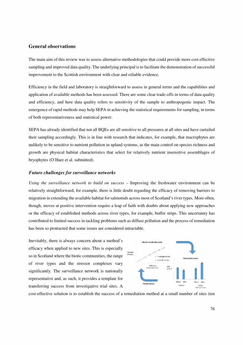
76
General observations
The main aim of this review was to assess alternative methodologies that could provide more cost effective
sampling and improved data quality. The underlying principal is to facilitate the demonstration of successful
improvement to the Scottish environment with clear and reliable evidence.
Efficiency in the field and laboratory is straightforward to assess in general terms and the capabilities and
application of available methods has been assessed. There are some clear trade-offs in terms of data quality
and efficiency, and here data quality refers to sensitivity of the sample to anthropogenic impact. The
emergence of rapid methods may help SEPA in achieving the statistical requirements for sampling, in terms
of both representativeness and statistical power.
SEPA has already identified that not all BQEs are all sensitive to all pressures at all sites and have curtailed
their sampling accordingly. This is in line with research that indicates, for example, that macrophytes are
unlikely to be sensitive to nutrient pollution in upland systems, as the main control on species richness and
growth are physical habitat characteristics that select for relatively nutrient insensitive assemblages of
bryophytes (O’Hare et al. submitted).
Future challenges for surveillance networks
Using the surveillance network to build on success – Improving the freshwater environment can be
relatively straightforward; for example, there is little doubt regarding the efficacy of removing barriers to
migration in extending the available habitat for salmonids across most of Scotland’s river types. More often,
though, moves at positive intervention require a leap of faith with doubts about applying new approaches
or the efficacy of established methods across river types, for example, buffer strips. This uncertainty has
contributed to limited success in tackling problems such as diffuse pollution and the process of remediation
has been so protracted that some issues are considered intractable.
Inevitably, there is always concern about a method’s
efficacy when applied to new sites. This is especially
so in Scotland where the biotic communities, the range
of river types and the stressor complexes vary
significantly. The surveillance network is nationally
representative and, as such, it provides a template for
transferring success from investigative trial sites. A
cost-effective solution is to establish the success of a remediation method at a small number of sites (ten
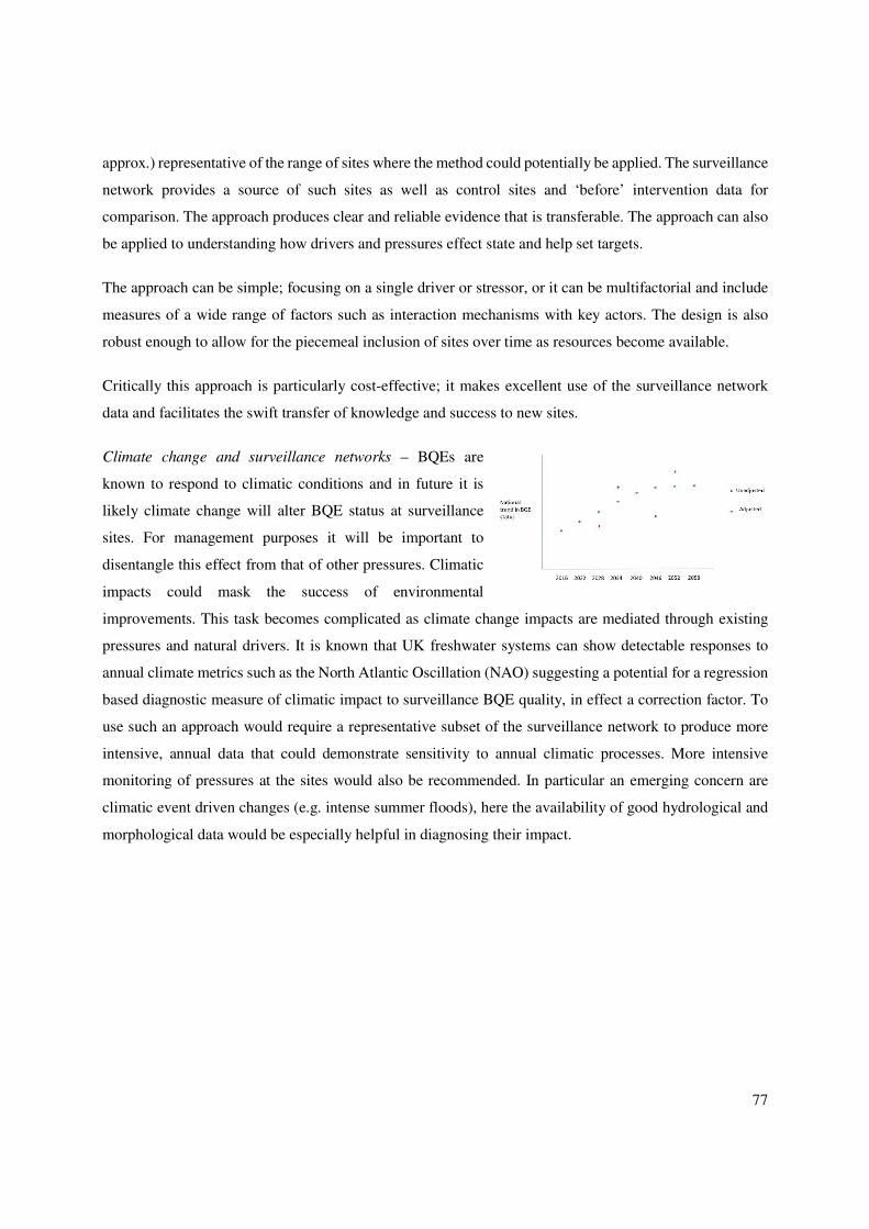
77
approx.) representative of the range of sites where the method could potentially be applied. The surveillance
network provides a source of such sites as well as control sites and ‘before’ intervention data for
comparison. The approach produces clear and reliable evidence that is transferable. The approach can also
be applied to understanding how drivers and pressures effect state and help set targets.
The approach can be simple; focusing on a single driver or stressor, or it can be multifactorial and include
measures of a wide range of factors such as interaction mechanisms with key actors. The design is also
robust enough to allow for the piecemeal inclusion of sites over time as resources become available.
Critically this approach is particularly cost-effective; it makes excellent use of the surveillance network
data and facilitates the swift transfer of knowledge and success to new sites.
Climate change and surveillance networks – BQEs are
known to respond to climatic conditions and in future it is
likely climate change will alter BQE status at surveillance
sites. For management purposes it will be important to
disentangle this effect from that of other pressures. Climatic
impacts could mask the success of environmental
improvements. This task becomes complicated as climate change impacts are mediated through existing
pressures and natural drivers. It is known that UK freshwater systems can show detectable responses to
annual climate metrics such as the North Atlantic Oscillation (NAO) suggesting a potential for a regression
based diagnostic measure of climatic impact to surveillance BQE quality, in effect a correction factor. To
use such an approach would require a representative subset of the surveillance network to produce more
intensive, annual data that could demonstrate sensitivity to annual climatic processes. More intensive
monitoring of pressures at the sites would also be recommended. In particular an emerging concern are
climatic event driven changes (e.g. intense summer floods), here the availability of good hydrological and
morphological data would be especially helpful in diagnosing their impact.

78
References
Baattrup-Pedersen, A., E. Gothe, S. E. Larsen, M. O'Hare, S. Birk, T. Riis, and N. Friberg. 2015. Plant trait
characteristics vary with size and eutrophication in European lowland streams. Journal of Applied
Ecology 52:1617-1628.
Baattrup-Pedersen, A., E. Gothe, T. Riis, D. K. Andersen, and S. E. Larsen. 2017. A new paradigm for
biomonitoring: an example building on the Danish Stream Plant Index. Methods in Ecology and
Evolution 8:297-307.
Baattrup-Pedersen, A., E. Gothe, T. Riis, and M. T. O'Hare. 2016. Functional trait composition of aquatic
plants can serve to disentangle multiple interacting stressors in lowland streams. Science of the
Total Environment 543:230-238.
Baattrup-Pedersen, A., S. E. Larsen, and T. Riis. 2013. From expert judgement to supervised classification:
A new approach to assess ecological status in lowland streams. Science of the Total Environment
447:116-122.
Baringhaus, L. and C. Franz. 2004. On a new multivariate two-sample test. Journal of Multivariate Analysis
88:190-206.
Bates, D., M. Mächler, B. M. Bolker, and S. C. Walker. 2015. Fitting Linear Mixed-Effects Models Using
lme4. Journal of Statistical Software 67:1-48.
Bennion, H., M. G. Kelly, S. Juggins, M. L. Yallop, A. Burgess, J. Jamieson, and J. Krokowski. 2014.
Assessment of ecological status in UK lakes using benthic diatoms. Freshwater Science 33:639-
654.
Birk, S., N. J. Willby, M. G. Kelly, W. Bonne, A. Borja, S. Poikane, and W. van de Bund. 2013.
Intercalibrating classifications of ecological status: Europe's quest for common management
objectives for aquatic ecosystems. Science of the Total Environment 454:490-499.
Bista, I., G. R. Carvalho, K. Walsh, M. Seymour, M. Hajibabaei, D. Lallias, M. Christmas, and S. Creer.
2017. Annual time-series analysis of aqueous eDNA reveals ecologically relevant dynamics of lake
ecosystem biodiversity. Nature Communications 8:14087.

79
Blamauer, B., B. Camenen, R. C. Grabowski, I. D. M. Gunn, A. M. Gurnell, H. Habersack, A. Latapie, M.
T. O'Hare, M. Palma, N. Surian, and L. Zilani. 2014. Catchment Case Studies:Partial Apllications
of the Hierarchical Multi-scale Framework.Deliverable 2.1, Part 4 of REFORM funded by the
European Commission within the 7th Framework programme under Grant Agreement 282656.
Bolker, B. M., M. E. Brooks, C. J. Clark, S. W. Geange, J. R. Poulsen, M. H. H. Stevens, and J.-S. S. White.
2009. Generalized linear mixed models: a practical guide for ecology and evolution. Trends in
Ecology & Evolution 24:127-135.
Bowes, M. J., H. P. Jarvie, S. J. Halliday, R. A. Skeffington, A. J. Wade, M. Loewenthal, E. Gozzard, J. R.
Newman, and E. J. Palmer-Felgate. 2015. Characterising phosphorus and nitrate inputs to a rural
river using high-frequency concentration–flow relationships. Science of the Total Environment
511:608-620.
Bowes, M. J., M. Loewenthal, D. S. Read, M. G. Hutchins, C. Prudhomme, L. K. Armstrong, S. A. Harman,
H. D. Wickham, E. Gozzard, and L. Carvalho. 2016. Identifying multiple stressor controls on
phytoplankton dynamics in the River Thames (UK) using high-frequency water quality data.
Science of the Total Environment 569:1489-1499.
Bowes, M. J., E. J. Palmer-Felgate, H. P. Jarvie, M. Loewenthal, H. D. Wickham, S. A. Harman, and E.
Carr. 2012. High-frequency phosphorus monitoring of the River Kennet, UK: are ecological
problems due to intermittent sewage treatment works failures? Journal of Environmental
Monitoring 14:3137-3145.
Bowes, M. J., J. T. Smith, and C. Neal. 2009. The value of high-resolution nutrient monitoring: a case study
of the River Frome, Dorset, UK. Journal of Hydrology 378:82-96.
Carvalho, L., S. Poikane, A. L. Solheim, G. Phillips, G. Borics, J. Catalan, C. De Hoyos, S. Drakare, B. J.
Dudley, M. Jarvinen, C. Laplace-Treyture, K. Maileht, C. McDonald, U. Mischke, J. Moe, G.
Morabito, P. Noges, T. Noges, I. Ott, A. Pasztaleniec, B. Skjelbred, and S. J. Thackeray. 2013.
Strength and uncertainty of phytoplankton metrics for assessing eutrophication impacts in lakes.
Hydrobiologia 704:127-140.
CEN. 2004. Guidance Standard for the Routine Analysis of Phytoplankton Abundance and Composition
using Inverted Microscopy (Utermohl technique). CEN/TC230/WG2/TG3. Comité Européen de
Normalisation, Geneva.

80
CEN. 2007. Guidance standard for surveying of macrophytes in lakes. CEN 15460: 2007. Comité Européen
de Normalisation, Geneva.
CEN. 2008. Phytoplankton Biovolume Determination by Microscopic Measurement of Cell Dimensions.
CEN/TC230/WG2/TG3. Comité Européen de Normalisation, Geneva.
CEN. 2011. Water Quality – Guidance Standard on assessing the hydromorphological features of
lakes.EN16039:2011. Comité Européen de Normalisation, Geneva.
Ciamittello, M., C. Dresti and H. Siadi. 2017. A review of Assessment approaches for Lake
Hydromorphology Before and After the European Water Framework Directive (WFD). Current
World Environment 12:491-506.
Civade, R., T. Dejean, A. Valentini, N. Roset, J. C. Raymond, A. Bonin, P. Taberlet, and D. Pont. 2016.
Spatial Representativeness of Environmental DNA Metabarcoding Signal for Fish Biodiversity
Assessment in a Natural Freshwater System. PLoS ONE 11(6):e0157366.
Cohen, J. 1988. Statistical power analysis for the behavioral sciences. Hilsdale. NJ: Lawrence Earlbaum
Associates.
Cohen, M. J., M. J. Kurz, J. B. Heffernan, J. B. Martin, R. L. Douglass, C. R. Foster, and R. G. Thomas.
2013. Diel phosphorus variation and the stoichiometry of ecosystem metabolism in a large spring-
fed river. Ecological Monographs 83:155-176.
Dashkova, V., D. Malashenkov, N. Poulton, I. Vorobjev, and N. S. Barteneva. 2017. Imaging flow
cytometry for phytoplankton analysis. Methods 112:188-200.
Deiner, K. and F. Altermatt. 2014. Transport Distance of Invertebrate Environmental DNA in a Natural
River. PLoS ONE 9 (2): e88786.
Deiner, K., E. A. Fronhofer, E. Machler, J. C. Walser, and F. Altermatt. 2016. Environmental DNA reveals
that rivers are conveyer belts of biodiversity information. Nature Communications 7:1-9.
De Nicola, D. M. and M. Kelly. 2014. Role of periphyton in ecological assessment of lakes. Freshwater
Science 33:619-638.
Di Stefano, J. 2003. How much power is enough? Against the development of an arbitrary convention for
statistical power calculations. Functional Ecology 17:707-709.

81
Dougherty, M. M., E. R. Larson, M. A. Renshaw, C. A. Gantz, S. P. Egan, D. M. Erickson, and D. M.
Lodge. 2016. Environmental DNA (eDNA) detects the invasive rusty crayfish Orconectes rusticus
at low abundances. Journal of Applied Ecology 53:722-732.
Elbrecht, V., A. J. Beermann, G. Goessler, J. Neumann, R. Tollrian, R. Wagner, A. Wlecklik, J. J. Piggott,
C. D. Matthaei, and F. Leese. 2016. Multiple-stressor effects on stream invertebrates: a mesocosm
experiment manipulating nutrients, fine sediment and flow velocity. Freshwater Biology 61:362-
375.
Elbrecht, V. and F. Leese. 2015. Can DNA-Based Ecosystem Assessments Quantify Species Abundance?
Testing Primer Bias and Biomass-Sequence Relationships with an Innovative Metabarcoding
Protocol. PLoS ONE 10 (7): e0130324.
Elbrecht, V., E. Vamos, K. Meissner, J. Aroviita, and F. Lesse. 2017. Assessing strengths and weaknesses
of DNA metabarcoding based macroinvertebrate identification for routine stream monitoring. PeerJ
Preprints https://doi.otg/10.7287/peerj.preprints.2759v2.
Extence, C., D. Balbi, and R. Chadd. 1999. River flow indexing using British benthic macroinvertebrates:
a framework for setting hydroecological objectives. Regulated Rivers: Research and Management
15:543-574.
Fitch, B. 2017. The new Riverfly Partnership host is... Pages 13-15 FBA News. The Freshwater Biological
Association.
Friberg, N., L. Sandin, M. T. Furse, S. E. Larsen, R. T. Clarke, and P. Haase. 2006. Comparison of
macroinvertebrate sampling methods in Europe. Hydrobiologia 566:365-378.
Furse, M. T., D. Hering, K. Brabec, A. Buffagni, L. Sandin, and P. F. M. Verdonschot. 2006. The ecological
status of European rivers: evaluation and intercalibration of assessment methods. Hydrobiologia
566:1-2.
Good, P. 2013. Permutation tests: a practical guide to resampling methods for testing hypotheses. Springer
Science & Business Media.
Halliday, S. J., R. A. Skeffington, M. J. Bowes, E. Gozzard, J. R. Newman, M. Loewenthal, E. J. Palmer-
Felgate, H. P. Jarvie, and A. J. Wade. 2014. The Water Quality of the River Enborne, UK:

82
Observations from High-Frequency Monitoring in a Rural, Lowland River System. Water 6:150-
180.
Halliday, S. J., R. A. Skeffington, A. J. Wade, M. J. Bowes, E. Gozzard, J. R. Newman, M. Loewenthal, E.
J. Palmer-Felgate, and H. P. Jarvie. 2015. High-frequency water quality monitoring in an urban
catchment: hydrochemical dynamics, primary production and implications for the Water
Framework Directive. Hydrological Processes 29:3388-3407.
Hanfling, B., L. L. Handley, D. S. Read, C. Hahn, J. L. Li, P. Nichols, R. C. Blackman, A. Oliver, and I. J.
Winfield. 2016. Environmental DNA metabarcoding of lake fish communities reflects long-term
data from established survey methods. Molecular Ecology 25:3101-3119.
Hellsten, S. and J. Riihimäki. 1996. Effects of lake water level regulation on the dynamics of littoral
vegetation in northern Finland. Hydrobiologia 340:85-92.
Helwig, K., J. Craft, P. Teedon, O. Pahl, and R. Allan. 2015. Inspiring Aquatic Monitoring: A review of
innovative approaches to monitoring the aquatic environment. CD2014_20.
Herder, J. E., A. Valentini, E. Bellemain, T. Dejean, J. J. C. W. van Delft, P. F. Thomsen, and P. Taberlet.
2014. Environmental DNA - a review of the possible applications for the detection of (invasive)
species. Report 2013-104, Strichting RAVON, Nijmegen.
Navico. 2014. BioBase User Reference Guide, Minneapolis, MN, USA.
Irvine, K. M., K. Manlove, and C. Hollimon. 2012. Power analysis and trend detection for water quality
monitoring data. An application for the Greater Yellowstone Inventory and Monitoring Network.
Report NPS/GRYN/NRR-2012/556.
Jakobsen, H. H. and J. Carstensen. 2011. FlowCAM: Sizing cells and understanding the impact of size
distributions on biovolume of planktonic community structure. Aquatic Microbial Ecology 65:75-
87.
JNCC. 2015. Common Standards Monitoring Guidance for Freshwater Fauna. Joint Nature Conservation
Committee, Peterborough.
Johnson, P. C., S. J. Barry, H. M. Ferguson, and P. Müller. 2015. Power analysis for generalized linear
mixed models in ecology and evolution. Methods in Ecology and Evolution 6:133-142.

83
Jones, I. D., I. J. Winfield, and F. Carse. 2008. Assessment of long-term changes in habitat availability for
Arctic charr (Salvelinus alpinus) in a temperate lake using oxygen profiles and hydroacoustic
surveys. Freshwater Biology 53:393-402.
Joutsijoki, H., K. Meissner, M. Gabbouj, S. Kiranyaz, J. Raitoharju, J. Auml;rje, S. Karkkainen, V.
Tirronen, T. Turpeinen, and M. Juhola. 2014. Evaluating the performance of artificial neural
networks for the classification of freshwater benthic macroinvertebrates. Ecological Informatics
20:1-12.
Kelly, M. G., J. Krokowski, and J. P. C. Harding. 2016. RAPPER: A new method for rapid assessment of
macroalgae as a complement to diatom-based assessments of ecological status. Science of the Total
Environment 568:536-545.
Kuznetsova, A., P. B. Brockhoff, and R. H. B. Christensen. 2015. Package ‘lmerTest’. R package version
2.
Lehtomäki, J. and A. Moilanen. 2013. Methods and workflow for spatial conservation prioritization using
Zonation. Environmental Modelling & Software 47:128-137.
Levine, C. R., R. D. Yanai, G. G. Lampman, D. A. Burns, C. T. Driscoll, G. B. Lawrence, J. A. Lynch, and
N. Schoch. 2014. Evaluating the efficiency of environmental monitoring programs. Ecological
Indicators 39:94-101.
Lindenmayer, D. B. and G. E. Likens. 2010. The science and application of ecological monitoring.
Biological Conservation 143:1317-1328.
Lovett, G. M., D. A. Burns, C. T. Driscoll, J. C. Jenkins, M. J. Mitchell, L. Rustad, J. B. Shanley, G. E.
Likens, and R. Haeuber. 2007. Who needs environmental monitoring? Frontiers in Ecology and the
Environment 5:253-260.
Miler, O., G. Porst, E. McGoff, F. Pilotto, L. Donohue, T. Jurca, A. Solimni, L. Sandin, K. Irvine, J.
Arvoviita, R. Clarke and M T. Pusch. Morphological alterations of lake shores in Europe: A
multimetric ecological assessment approach using benthic invertebrates. Ecological Indicators 34:
398-410.

84
Moilanen, A., A. M. Franco, R. I. Early, R. Fox, B. Wintle, and C. D. Thomas. 2005. Prioritizing multiple-
use landscapes for conservation: methods for large multi-species planning problems. Proceedings
of the Royal Society of London B: Biological Sciences 272:1885-1891.
O'Hare, J. M., M. T. O'Hare, A. M. Gurnell, M. J. Dunbar, P. M. Scarlett, and C. Laize. 2011. Physical
constraints on the distribution of macrophytes linked with flow and sediment dynamics in British
rivers. River Research and Applications 27:671-683.
O'Hare, M. T., R. T. Clarke, M. J. Bowes, C. Cailes, P. Henville, N. Bissett, C. McGahey, and M. Neal.
2010. Eutrophication impacts on a river macrophyte. Aquatic Botany 92:173-178.
O'Hare, M. T., A. Baattrup-Pedersen, I. Baumgarte, A. Freeman, I. D. M. Gunn, A. N, Lázár, R. Sinclair,
A. J. Wade and M. J. Bowes. Submitted. Responses of aquatic plants to eutrophication in rivers.
Frontiers in Science.
Pires, M. D. 2010. Evaluation of flurometers for the in situ monitoring of chlorophyll and/or cyanobacteria.
Report reference 1203593-000-ZWS-0004, Deltares, the Netherlands.
Poikane, S., S. Birk, J. Bohmer, L. Carvalho, C. de Hoyos, H. Gassner, S. Hellsten, M. Kelly, A. L. Solheim,
M. Olin, K. Pall, G. Phillips, R. Portielje, D. Ritterbusch, L. Sandin, A. K. Schartau, A. G. Solimini,
M. van den Berg, G. Wolfram, and W. van de Bund. 2015. A hitchhiker's guide to European lake
ecological assessment and intercalibration. Ecological Indicators 52:533-544.
R Core Team. 2017. R package stats: A language and environment for statistical computing.
Read, D. et al. 2017. A review of the application of molecular approaches for describing biodiversity, in
the context of CEH research and monitoring. Draft Centre for Ecology & Hydrology Report.
Read, D. S., M. J. Bowes, L. K. Newbold, and A. S. Whiteley. 2014. Weekly flow cytometric analysis of
riverine phytoplankton to determine seasonal bloom dynamics. Environmental Science-Processes
& Impacts 16:594-603.
Rinaldi, M., B. Belletti, W. Van de Bund, W. Bertoldi, A. Gurnell, T. Buijse, and E. Mosselman. 2013.
Review on eco-hydromorphological methods . Deliverable 1.1. of REFORM funded by the
European Commission within the 7th Framework programme under Grant Agreement 282656.
Rode, M., A. J. Wade, M. J. Cohen, R. T. Hensley, M. J. Bowes, J. W. Kirchner, G. B. Arhonditsis, P.
Jordan, B. Kronvang, S. J. Halliday, R. A. Skeffington, J. C. Rozemeijer, A. H. Aubert, K. Rinke,

85
and S. Jomaa. 2016. Sensors in the Stream: The High-Frequency Wave of the Present.
Environmental Science & Technology 50:10297-10307.
SEPA. 2007. Scotland’s WFD aquatic monitoring strategy Scottish Environment Protection Agency,
Stirling, UK.
SNIFFER. 2008a. Development of Lake-MImAS as a decision-support tool for managing
hydromorphological alterations to lakes.1-70.
SNIFFER. 2008b. Lake habitat survey in the United Kingdom - Field survey guidance manual, version 4.
1-79.
Solimini, A. G., G. Free, I. Donohue, K. Irvine, M. Pusch, B. Rossaro, L. Sandin, and A. C. Cardoso. 2006.
Using Benthic Macroinvertebrates to Assess Ecological Status of Lakes. Office for Official
Publications of the European Communities. EUR22347 EN, Luxembourg.
Solimini, A. G. and L. Sandin. 2012. The importance of spatial variation of benthic invertebrates for the
ecological assessment of European lakes. Fundamental and Applied Limnology 180:85-89.
Spears, B. M., I. D. M. Gunn, L. Carvalho, I. J. Winfield, B. Dudley, K. Murphy, and L. May. 2009. An
evaluation of methods for sampling macrophyte maximum colonisation depth in Loch Leven,
Scotland. Aquatic Botany 91:75-81.
Spyrakos, E., R. O'Donnell, P. D. Hunter, C. Miller, M. Scott, S. G. Simis, C. Neil, C. F. Barbosa, C. E.
Binding, S. Bradt, M. Bresciani, G. Dall'Olmo, C. Giardino, A. A. Gitelson, T. Kuser, L. Li, B.
Matsushita, V. Martinez-Vicente, M. W.Matthews, I. Ogashawara, A. Ruiz-Verdú, J. F. Schalles,
E. Tebbs, Y. Zhang and A. N. Tyler 2017. Optical types of inland and coastal waters. Limnology
and Oceanography. DOI:10.1002/Ino.10674.
Telford, A., M. T. O'Hare, S. Cavers, and N. Holmes. 2011. Can genetic bar-coding be used to identify
aquatic Ranunculus L. subgenus Batrachium (DC) A. Gray? A test using some species from the
British Isles. Aquatic Botany 95:65-70.
The Scottish Government. 2014. The Scotland River Basin District (Standards) Directions 2014.
Edinburgh, UK.

86
Tyler, A. N., P. D. Hunter, E. Spyrakos, S. Groom, A. M. Constantinescu, and J. Kitchen. 2016.
Developments in Earth observation for the assessment and monitoring of inland, transitional,
coastal and shelf-sea waters. Science of the Total Environment 572:1307-1321.
Valley, R. D., M. T. Drake, and C. S. Anderson. 2005. Evaluation of alternative interpolation techniques
for the mapping of remotely-sensed submersed vegetation abundance. Aquatic Botany 81:13-25.
Valley, R. D., M. B. Johnson, D. L. Dustin, K. D. Jones, M. R. Lauenstein, and J. Nawrocki. 2015.
Combining hydroacoustic and point-intercept survey methods to assess aquatic plant species
abundance patterns and community dominance. Journal of Aquatic Plant Management 53:121-129.
Warton, D. I. and F. K. C. Hui. 2011. The arcsine is asinine: the analysis of proportions in ecology. Ecology
92:3-10.
WFD-UKTAG. 2008a. UKTAG Lake Assessment Methods: Benthic Invertebrate Fauna. Chironomid
Pupal Exuviae Technique (CPET). Edinburgh.
WFD-UKTAG. 2008b. UKTAG Lake Assessment Methods: Benthic Invertebrate Fauna: Lake
Acidification Macroinvertebrate Metric (LAMM). Edinburgh.
WFD-UKTAG. 2014a. UKTAG River Assessment Method: Macrophytes and Phytobenthos. Macrophytes
(River LEAFPACS2). Stirling.
WFD-UKTAG. 2014b. UKTAG River Assessment Method: Macrophytes and Phytobenthos. Phytobenthos
- Diatoms for Assessing River and Lake Ecological Quality (River DARLEQ2). Stirling.
WFD-UKTAG. 2014c. UKTAG River Assessment Method: Benthic Invertebrate Fauna. Invertebrates
(General Degradation): Whalley, Hawkes, Paisley & Trigg (WHPT) metric on River Invertebrate
Classification Tool (RICT). Stirling.
WFD-UKTAG. 2014d. UKTAG River Assessment Method: Fish Fauna. Fish Classification Scheme 2
(FCS2) Scotland. Stirling.
WFD-UKTAG. 2014e. UKTAG Lake Assessment Method: Macrophytes and Phytobenthos. Macrophytes
(Lake LEAFPACS). Stirling.
WFD-UKTAG. 2014f. UKTAG Lake Assessment Method Phytoplankton: Phytoplankton Lake
Assessment Tool with Uncertainty Module (PLUTO). Stirling.

87
WFD-UKTAG. 2014g. UKTAG Lake Assessment Method: Macrophytes and Phytobenthos. Phytobenthos
- Diatoms for Assessing River and Lake Ecological Quality (Lake DARLEQ2). WFD-UKTAG,
Stirling.
Winfield, I. J., C. E. Adams, C. W. Bean, N. C. Durie, J. M. Fletcher, A. R. Gowans, C. Harrod, J. B. James
, A. A. Lyle, P. S. Maitland, C. Thompson, and E. Verspoor. 2012. Conservation of the vendace
(Coregonus albula), the UK's rarest freshwater fish. Advances in Limnology 63:547-559.
Winfield, I. J., C. W. Bean, J. Gorst, A. R. D. Gowans, M. Robinson, and R. Thomas. 2013. Assessment
and conservation of whitefish (Coregonus lavaretus (L.)) in the UK. Advances in Limnology
64:305-321.
Winfield, I. J., J. M. Fletcher, and J. B. James. 2007a. Seasonal variability in the abundance of Arctic charr
(Salvelinus alpinus (L.)) recorded using hydroacoustics in Windermere, UK and its implications
for survey design. Ecology of Freshwater Fish 16:64-69.
Winfield, I. J., J. M. Fletcher, J. B. James, and C. W. Bean. 2009. Assessment of fish populations in still
waters using hydroacoustics and survey gill netting: Experiences with Arctic charr (Salvelinus
alpinus) in the UK. Fisheries Research 96:30-38.
Winfield, I. J., C. Onoufriou, M. J. O'Connell, M. Godlewska, R. M. Ward, A. F. Brown, and M. L. Yallop.
2007b. Assessment in two shallow lakes of a hydroacoustic system for surveying aquatic
macrophytes. Hydrobiologia 584:111-119.
Winfield, I. J., J. van Rijn, and R. D. Valley. 2015. Hydroacoustic quantification and assessment of
spawning grounds of a lake salmonid in a eutrophicated water body. Ecological Informatics 30:235-
240.
Wood, K. A., R. A. Stillman, R. T. Clarke, F. Daunt, and M. T. O'Hare. 2012. Measuring submerged
macrophyte standing crop in shallow rivers: A test of methodology. Aquatic Botany 102:28-33.
Wood, S. and F. Scheipl. 2017. gamm4: Generalized additive mixed models using mgcv and lme4. R
package version 0.2-5.
Wright, J. F., D. W. Sutcliffe and M. T. Furse. 2000. Assessing the biological quality of fresh waters:
RIVPACS and other techniques. Freshwater Biologicial Association, Ambleside.

88
Appendices
Appendix 2.1: Priority water bodies for removal from the river
surveillance network
Table A1. Prioritisation for removal of water bodies from the existing river surveillance network, based
solely on increasing representativeness (1=highest priority to remove).
Removal
priority
Water body
code
Water body name
1 10919 River Clyde (Mouse Water to Strathclyde Loch outflow)
2 6498 River Tay (R Isla to R Earn Confluences)
3 5200 River Tweed (Coldstream to tidal limit)
4 5202 River Tweed (Ettrick Water to St Boswells Burn confluences)
5 10042 River Clyde (Potrail Water to Mouse Water)
6 6521 River Isla (R Ericht to R Tay Confluences)
7 10642 River Annan (Threewaterfoot to Annan)
8 23065 River Spey - R. Fiddich to tidal limit
9 4700 River Forth (below R. Teith confluence)
10 6800 River Earn
11 23265 River Don - Dyce to tidal limit
12 10610 River Nith (Dumfries - Sanquhar)
13 10918 River Clyde (Strathclyde Loch outflow to North Calder)
14 6499 River Tay (R Tummel to R Isla Confluences)
15 10420 River Ayr (d/s Greenock Water)
16 10391 River Irvine (Cessnock conf to Tidal Weir)
17 10150 River Leven
18 23155 River Deveron - Turriff to tidal limit
19 5799 River South Esk (White Burn Confluence to Estuary)
20 5219 Teviot Water (Kale Water confluence to River Tweed)
21 23066 River Spey - R. Avon to R. Fiddich
22 5203 River Tweed (Scotsmill to Ettrick Water confluence)
23 10758 River Esk (Black Esk to National Boundary)
24 3000 River Almond (Maitland Bridge to Cramond)
25 23165 River Deveron - Huntly to Turriff

89
Removal
priority
Water body
code
Water body name
26 23315 River Dee - Peterculter to tidal limit
27 5700 River North Esk (Confluence with Cruick Water to Estuary)
28 5220 Teviot Water (Northhouse Burn to Kale Water confluences)
29 10000 White Cart Water (Kittoch Water to A726 road bridge)
30 5204 River Tweed (Talla Water confluence to Scotsmill)
31 6838 River Earn (Water of Ruchill to Ruthven Water confluences)
32 10130 River Kelvin (Glazert Water to Tidal Limit)
33 23096 River Spey - R. Nethy to R. Avon
34 3800 River Esk
35 23293 River Don - Alford to Inverurie
36 4000 River Tyne (Birns Water confluence to Estuary)
37 10427 Lugar Water
38 23332 River Dee - Ballater to Banchory
39 10924 River Doon (d/s Muck Water)
40 6832 Allan Water d/s of Dunblane
41 6828 River Tummel (L Faskally to R Tay)
42 4500 River Devon (Gairney Burn confluence to Estuary)
43 23231 River Ythan - Methlick to Ellon
44 6834 River Teith
45 3801 River South Esk (Gore Water to N Esk confluences)
46 10545 River Dee (Loch Ken Outlet to Tongland)
47 10152 Endrick Water (d/s Blane Water)
48 6500 River Tay (R Lyon to R Tummel Confluences)
49 4200 River Carron (Bonny Water confluence to Carron Estuary)
50 20339 River Lochy - sea to Spean confluence
51 10076 Avon Water (Powmillon Burn to River Clyde)
52 20165 River Conon - Cromarty Firth to Orrin confluence
53 6200 River Eden (Confluence with Rossie Drain to Estuary)
54 10757 Water of Girvan (d/s Dailly)
55 10747 Black Cart Water
56 6844 Whiteadder Water (Billie Burn confluence to tidal limit)
57 23171 River Isla - d/s Shiel Burn
58 5287 Ettrick Water (Ramseycleuch to River Tweed)
59 23394 River Ness - Inverness Firth to Loch Ness
60 10092 Douglas Water (Poneil to Clyde)

90
Removal
priority
Water body
code
Water body name
61 6523 River Isla (Glencally Burn to Dean Water Confluences)
62 23282 River Urie - Lochter Burn to Don
63 23345 River Dee - Braemar to Ballater
64 10379 River Garnock (Caaf Water to Tidal Limit)
65 6506 River Almond (R East Pow to R Tay Confluences)
66 23232 River Ythan - Fyvie to Methlick
67 3100 River Avon (Logie Water confluence to Estuary)
68 6555 Dean Water (Kerbet Water to R Isla Confluences)
69 20637 River Thurso - Loch More to sea
70 6836 River Garry (Errochty Water Confluence to L Faskally)
71 23188 River Bogie - Culdrain to Huntly
72 10465 River Stinchar (d/s Duisk River)
73 23000 River Findhorn - Dorback Burn to sea
74 23215 River Ugie - North/South confl to tidal limit
75 5705 Luther Water ( Dowrie Burn to North Esk Confluences)
76 23142 River Spey - Spey Dam to Loch Insh
77 10394 Annick Water
78 23294 River Don - Strathdon to Alford
79 6300 River Leven (Markinch to Estuary)
80 10280 River Awe
81 10030 River Gryfe (d/s Barochan Burn)
82 5266 Leader Water/Kelphope Burn (Cleekhimin Burn confluence to River
Tweed)
83 20209 River Beauly - Beauly Firth to Cannich
84 23032 River Lossie - Waukmill to Arthurs Bridge
85 10060 North Calder Water (Luggie Burn to Clyde)
86 6501 River Tay (Loch Tay to R Lyon Confluence)
87 23283 River Urie - Pitcaple to Lochter Burn
88 10153 Endrick Water (u/s Blane Water)
89 10040 River Clyde (North Calder to Tidal Weir)
90 23084 River Avon / River Livet - lower catchment
91 4704 River Forth (Milton to Auchentroig Burn confluence)
92 5701 River North Esk ( Water of Effock to Cruick Water Confluences)
93 10001 White Cart Water (above Kittoch conf)
94 10520 River Cree (u/s Newton Stewart)

91
Removal
priority
Water body
code
Water body name
95 5105 Blackadder Water (Howe Burn confluence to Whiteadder Water)
96 20305 River Nairn - Moray Firth to River Farnack confluence
97 20036 Wick River - Loch Watten Burn to tidal limit
98 23004 River Findhorn - Tomatin to Dorback Burn
99 6301 River Leven (Loch Leven to Markinch)
100 3806 River North Esk (Elginhaugh to confluence with South Esk)
101 20167 River Conon - Loch Achonachie to Loch Luichart
102 10666 Kirtle Water (d/s Waterbeck)
103 20116 River Oykel - Dornoch Firth to Loch Craggie
104 23264 Bervie Water - lower catchment
105 10491 Water of Luce (d/s Cross Water of Luce)
106 20002 River Helmsdale - Kinbrace Burn to sea
107 10072 South Calder Water (Tillan Burn to Strathclyde Park)
108 5236 Ale Water (Woll Burn confluence to Teviot Water)
109 6502 River Dochart (Confluence Auchlyne West Burn to Loch Tay)
110 10101 Medwin Water
111 23326 Water of Feugh - lower catchment
112 10761 Water of Ken
113 5311 Lyne Water (Tarth Water confluence to River Tweed)
114 20057 River Brora - sea to Loch Brora
115 10285 River Orchy
116 5101 Whiteadder Water (Dye Water to Billie Burn confluences)
117 23224 South Ugie Water - Stuartfield to Longside
118 20093 River Shin - Dornoch Firth to Loch Shin
119 3700 Water of Leith (Murray Burn confluence to Estuary)
120 20595 River Naver - sea to Loch Naver
121 10422 Water of Coyle (d/s Taiglum Burn)
122 6535 R Ericht
123 10583 Urr Water (d/s Drumhumphrey Burn)
124 5222 Kale Water
125 10205 River Eachaig
126 6839 River Earn (Loch Earn to Water of Ruchill confluence)
127 5280 Gala Water (Armet Water confluence to River Tweed)
128 6639 River Lyon
129 5215 Eden Water (Hume Burn confluence to River Tweed)

92
Removal
priority
Water body
code
Water body name
130 10156 Blane Water/Ballagan Burn
131 6585 River Tummel (Dunalastair Water to Loch Tummel)
132 10645 Water of Milk (d/s Corrie Water Confluence)
133 20262 River Enrick - Loch Ness to Loch Meiklie
134 20633 Forss Water - Allt Forsiescye to sea
135 6586 River Tummel (Loch Rannoch to Dunalastair Water)
136 10657 Water of Ae (d/s Goukstane Burn)
137 6000 Dighty Water (lower)
138 10927 Cessnock Water
139 20412 River Shiel - sea to Loch Shiel
140 5290 Yarrow Water
141 10080 Nethan Water
142 20010 River Helmsdale - Loch Badanloch to Kinbrace Burn
143 10084 Mouse Water (Dippool Water to Clyde)
144 20483 River Ewe - sea to Loch Maree
145 20156 Alness River - Cromarty Firth to Strone
146 10469 Duisk River (d/s Muck Water Confluence)
147 5900 Lunan Water (Friockheim to Estuary)
148 5231 Jed Water/Raven Burn (Kaim Burn confluence to Teviot Water)
149 20130 River Carron - sea to Alladale Lodge
150 10399 Kingswell Burn/Fenwick Water/Kilmarnock Water
151 20110 River Cassley - Dornoch Firth to Glenmuick
152 23106 River Dulnain - lower catchment
153 5207 Leet Water (Lambden Burn confluence to River Tweed)
154 6576 River Braan
155 23579 River Borgie d/s Loch Craggie
156 10383 Lugton Water
157 10315 River Etive (d/s Allt a Chaorainn)
158 10132 Allander Water
159 20410 River Aline
160 23346 River Dee - White Bridge to Braemar
161 10073 South Calder Water (Auchter Water to Tillan Burn)
162 20614 Halladale River - d/s Forsinain Burn
163 20254 River Garry - Loch Oich to Loch Garry
164 10589 Kirkgunzeon Lane

93
Removal
priority
Water body
code
Water body name
165 10612 River Nith (u/s New Cumnock)
166 20733 River Snizort
167 23221 North Ugie Water - lower catchment
168 10521 River Cree (u/s Minnoch conf)
169 4202 River Carron (Carron Valley Reservoir to Avon Burn Confluence)
170 23233 River Ythan - upper catchment above Fyvie
171 20586 River Hope
172 10546 Black Water of Dee (Pullaugh Burn to Loch Ken)
173 5010 Eye Water (Ale Water Confluence to Eyemouth)
174 23371 River Carron - Loch Carron to Loch Dughaill
175 4402 Black Devon (Birkhill Plantation to Forth Estuary)
176 20451 River Ling - sea to Aonach Beag
177 20317 Muckle Burn - Lethen to Speedie Burn
178 10514 Tarf Water (u/s Bladnoch)
179 20446 River Morar - sea to Loch Morar
180 6806 Ruthven Water
181 10562 Water of Deugh (Carsphairn Lane to Water of Ken)
182 3904 Biel Water
183 20558 River Inver - sea to Loch Assynt
184 10356 River Laggan
185 6102 Motray Water
186 23347 River Gairn - lower catchment
187 20330 River Leven - sea to Blackwater Reservoir
188 20099 River Tirry - Loch Shin to Rhian
189 10669 River Sark
190 10321 River Creran
191 23319 Culter Burn
192 20563 River Laxford - d/s Loch Stack
193 5603 Brothock Water
194 20505 Ullapool River
195 20547 River Broom
196 10539 Water of Fleet/Big Water of Fleet/Mid Burn
197 20542 Gruinard River
198 4008 Birns Water/Humbie Water
199 20047 Dunbeath Water - Burn of Houstry to sea

94
Removal
priority
Water body
code
Water body name
200 10300 River Nant (d/s Loch Nant)
201 5950 Elliot Water/Rottenraw Burn
202 23129 River Feshie - main stem d/s R. Eidart
203 6830 Bannock Burn (Sauchie Burn confluence to Steuarthall Farm)
204 10527 Water of Minnoch (River Cree to Water of Trool)
205 20111 River Cassley - Glenmuick to Fionn Loch Beag
206 23043 River Lossie - upper catchment
207 20387 River Scaddle / Cona River
208 10484 Piltanton Burn
209 20610 River Strathy - The Uair to sea
210 6108 Kenly Water (Confluence with Kinaldy Burn to Estuary)
211 20329 River Nevis
212 20053 Berriedale Water
213 5953 Barry Burn
214 20211 River Affric - Loch Beinn a Mheadhoin to Loch Affric
215 10493 Cross Water of Luce
216 6320 North Queich River
217 20572 River Dionard
218 23634 River Canaird (lower section) and Allt a' Mhuilinn
219 5228 Oxnam Water (River Teviot to Newbigging Burn)
220 20532 Allt Mor Gisgil
221 10492 Water of Luce (u/s Cross Water of Luce)
222 6107 Kinness Burn
223 23295 River Don - source to Strathdon
224 20823 Abhainn thernaraigh
225 20407 River Ailort
226 4001 River Tyne (Source to Birns Water confluence)
227 10446 Garpel Burn
228 20054 Langwell Water
229 10497 Milton Burn/Dergoals Burn
230 20433 River Elchaig
231 5952 Monikie Burn
232 20430 River Shiel
233 20642 Halkirk Burn
234 23187 River Deveron - source to Black Water confl.

95
Removal
priority
Water body
code
Water body name
235 10393 River Irvine (u/s Glen Burn)
236 4734 Drunkie Burn (Loch Drunkie sluice to Loch Venachar)
237 20095 Merkland River - Loch a Ghriama to Loch Merkland
238 10062 North Calder Water (d/s Hillend Reservoir to Shotts Burn)
239 6533 Leddown Burn/Lunan Burn (to Loch of Craiglush)
240 10145 Glazert Water/Finglen Burn
241 23154 River Spey - source to Garva
242 10536 Moneypool Burn
243 10220 River Shira (d/s Lochan Shira)
244 5954 Buddon Burn
245 20496 Allt Bad an Luig
246 5809 Prosen Water (Burn of Lednathie to South Esk Confluences)
247 20801 Abhainn Bharabhais
248 4206 Glencryan Burn
249 23127 River Feshie - Allt a Mharcaidh
254 4720 Calair Burn
254 5011 Eye Water (Source to Ale Water Confluence)
254 10343 Aros River/Ledmore River (d/s Loch Frisa)
254 10457 Water of Girvan (u/s Loch Bradan)
254 23222 North Ugie Water - upper catchment

96
Appendix 2.2: Priority water bodies for addition to the river
surveillance network
Table A2. Priority water bodies for addition to the river surveillance network, after initial reduction to
various sizes (1=highest priority to add). The table shows any water body in the top 25 priorities for any
one of the simulations. Dashes indicate that the water body was not added at all, that is priority > 250.
Water
body
code
Water body name Add to
existing
network
Add to
200
water
bodies
Add to
150
water
bodies
Add to
100
water
bodies
Add to
50
water
bodies
20214 Bruiach Burn - Loch Bruicheach to
source
2 1 1 1 -
20598 Meadie Burn 1 2 2 2 -
20123 Abhainn Poiblidh 3 3 4 - -
20231 Allt Coire Calavie 4 4 3 5 -
6625 River Ericht (Source to Loch Ericht near
Dalwhinnie)
7 6 6 3 1
4722 Drunkie Burn (Reoidhte Lochan to Loch
Drunkie)
10 7 5 4 2
6656 Lairig an Lochain 5 5 7 - -
20520 Allt Loch an Tuirc - Loch Crocach to
source
6 9 - - -
5310 Glenrath Burn - - - - 8
20497 Allt an Loch Fhada 8 8 9 - -
20499 Allt a Chladhain 9 10 - - -
20604 Mallart River - u/s Loch a Bhealaich 12 12 8 7 -
6658 Allt Breaclaich (Source to Breaclaich
Res)
11 11 - - -
20366 Allt Feith Thuill - - - - 12
6816 River Lednock 17 13 10 9 -
10447 Pollcrayvie Burn 18 14 12 8 -
10133 Craigmaddie Burn - - - - 13
23101 Cromdale Burn - - - - 14
20024 Allt an Loin Tharsuin - u/s Loch
Truderscaig
15 15 13 - -
4211 Auchenbowie Burn (Source to Loch
Coulter Reservoir)
25 19 11 6 -

97
Water
body
code
Water body name Add to
existing
network
Add to
200
water
bodies
Add to
150
water
bodies
Add to
100
water
bodies
Add to
50
water
bodies
20221 Allt Bealach an Sgoltaidh 14 17 15 - -
20788 Abhainn Giosla - u/s Loch Gruineabhat 13 18 - - -
20394 Savary River - - - - 16
10248 Allt Mor (u/s Loch Ciaran) 19 16 14 - -
20371 Allt Coire Pitridh 23 24 - - 3
10344 Allt a Chlogaid (u/s Loch Frisa) 16 21 - - -
10552 Cuttiemore Burn 31 26 16 10 -
20763 Abhainn Smuaisibhig - - - - 21
20829 Tarbert Burn 21 - - - -
23914 Allt Crunachdain 32 25 17 12 -
10548 Dargall Lane 20 20 25 - -
20284 Allt Phocaichain 34 30 23 16 6
20493 Allt Gleann Tulacha 22 - - - -
4707 Water of Chon (Source to Loch Chon) 28 23 19 - -
20364 Allt na Caplaich Mor 27 22 21 - -
10310 Abhainn Dalach - - - - 24
10329 Abhainn Tir Chonhuill/Allt an Fhir eoin 37 29 20 15 -
3501 Braid Burn (Source to Upstream
Dreghorn Barracks)
56 36 22 11 4
10325 Un-named trib of Loch Glashan 39 27 18 - -
23325 Burn of Corrichie - - 42 21 -
20314 Feith Ghlas 42 33 24 - -
10163 Carn Allt 48 37 33 23 -
20097 Allt na Fearna Mor 58 42 28 20 -
10592 Culloch Burn (u/s Milton Loch) 72 41 27 13 -
5300 Gatehopeknowe Burn 70 46 29 14 -
23134 Allt Na Baranachd 61 50 31 19 -
20704 Lon Coire na h-Airigh 85 - - 32 10
10095 Parkhall Burn 76 51 32 18 -
6825 Chesterknowes Burn - 119 - 33 5
23316 River Dee - Banchory to Peterculter - - - 91 20
23356 Crathie Burn 105 77 46 22 -
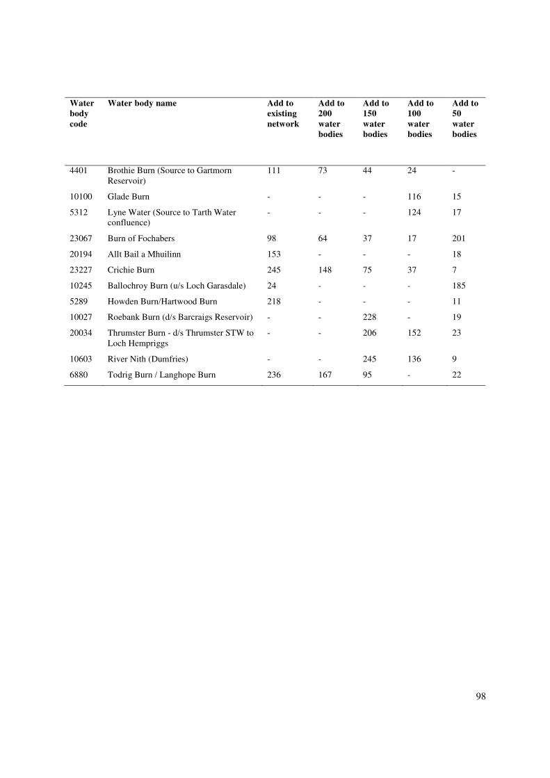
98
Water
body
code
Water body name Add to
existing
network
Add to
200
water
bodies
Add to
150
water
bodies
Add to
100
water
bodies
Add to
50
water
bodies
4401 Brothie Burn (Source to Gartmorn
Reservoir)
111 73 44 24 -
10100 Glade Burn - - - 116 15
5312 Lyne Water (Source to Tarth Water
confluence)
- - - 124 17
23067 Burn of Fochabers 98 64 37 17 201
20194 Allt Bail a Mhuilinn 153 - - - 18
23227 Crichie Burn 245 148 75 37 7
10245 Ballochroy Burn (u/s Loch Garasdale) 24 - - - 185
5289 Howden Burn/Hartwood Burn 218 - - - 11
10027 Roebank Burn (d/s Barcraigs Reservoir) - - 228 - 19
20034 Thrumster Burn - d/s Thrumster STW to
Loch Hempriggs
- - 206 152 23
10603 River Nith (Dumfries) - - 245 136 9
6880 Todrig Burn / Langhope Burn 236 167 95 - 22

99
Appendix 2.3 R code to analyse and improve the representativeness
of a monitoring network
This appendix contains R functions and code to test the representativeness of a monitoring network with
respect to multiple gradients and find sites to remove or add to the network in order to improve
representativeness.
The functions and R commands can be copied directly into R to implement a simplified workflow of the
analyses in Sections 1 and 2, using randomly-generated dummy data. Application to real data can be done
by formatting the real data to match the formats of the dummy data.
R Functions
network_KS_test = function(gradientData, network, numSimulations=1000){
# Function to run two-sample Kolmogorov-Smirnov test on gradient
distributions inside and outside of the network
# gradientData = data.frame of gradient values (rows=sites,
columns=gradients)
# network = Boolean vector of length equal to the rows in gradientData
coding whether each site is in the network (TRUE) or not (FALSE)
# numSimulations = number of simulations for randomisation test
testResults = t(sapply(1:ncol(gradientData), function(g){ # for each
gradient, run the test...
# calculate the observed KS statistic for difference between gradient
distributions
# inside and outside the network...
x_inNetwork = gradientData[network,g] # gradient values in the network
x_outNetwork = gradientData[!network,g] # gradient values not in the
network
KSD = suppressWarnings(ks.test(x_inNetwork, x_outNetwork)$statistic) # KS
d statistic
# generate simulated values of the KS statistic under the null hypothesis
# of no difference between sites inside and outside the network...
sim_KSD = sapply(1:numSimulations, function(dummy){
randNumber = runif(nrow(gradientData))
sim_inNetwork = randNumber < quantile(randNumber, mean(network)) #
simulated network (random sample of sites)
x_inNetwork = gradientData[sim_inNetwork,g] # gradient values in the
simulated network
x_outNetwork = gradientData[!sim_inNetwork,g] # gradient values not in
the simulated network
suppressWarnings(ks.test(x_inNetwork, x_outNetwork)$statistic) # KS d
statistic
})
# calculate the P value...
P = (1+sum(sim_KSD > KSD)) / (1+length(sim_KSD))

100
# return the result...
return(c(D=as.numeric(KSD), P=P))
}))
# return the results...
return(data.frame(gradient=names(gradientData), testResults))
}
network_Cramer_test = function(gradientData, network, numSimulations=1000){
# Function to run two-sample Cramer's test on gradient distributions
# inside and outside of the network
# gradientData = data.frame of gradient values (rows=sites,
columns=gradients)
# network = Boolean vector of length equal to the rows in gradientData
coding whether each site is in the network (TRUE) or not (FALSE)
# numSimulations = number of simulations for randomisation test
# transform gradient values to Gaussian distributions with mean=0 and
standard deviation=1...
require(GenABEL)
gradientDataT = apply(gradientData, 2, rntransform)
# compute pairwise Euclidean distance matrix on transformed gradients...
distanceMatrix = as.matrix(dist(gradientDataT))
# function to calculate Cramer's T statistic
cramersT = function(rep=NULL, DM, gp, permute=FALSE){
if(permute) gp = sample(gp)
nIn = sum(gp)
nOut = sum(!gp)
(nIn*nOut/(nIn+nOut)) * (sum(DM[!gp,gp])/(nIn*nOut) -
sum(DM[!gp,!gp])/(2*nOut*nOut) - sum(DM[gp,gp])/(2*nIn*nIn))
}
# calculate the observed T statistic for difference between gradient
distributions inside and outside the network...
CRT = cramersT(rep=NULL, DM=distanceMatrix, gp=network, permute=FALSE)
# generate simulated values of the T statistic under the null hypothesis of
no difference between sites inside and outside the network...
sim_CRT = sapply(1:numSimulations, cramersT, DM=distanceMatrix, gp=network,
permute=TRUE)
# calculate the P value...
P = (1+sum(sim_CRT > CRT)) / (1+length(sim_CRT))
# return the result...
return(c(CramersT=CRT, P=P))
}

101
stepwise_removal = function(gradientData, startNetwork, numRemovals=50){
# Function to run stepwise removal of sites from the monitoring network,
# to maximise representativeness (minimise Cramer's T)
# gradientData = data.frame of gradient values (rows=sites,
columns=gradients)
# startNetwork = Boolean vector of length equal to the rows in gradientData
coding whether each site is in the initial network (TRUE) or not
(FALSE)
# numRemovals = number of sites to remove
# transform gradient values to Gaussian distributions with mean=0 and
standard deviation=1...
require(GenABEL)
gradientDataT = apply(gradientData, 2, rntransform)
# compute pairwise Euclidean distance matrix on transformed gradients...
distanceMatrix = as.matrix(dist(gradientDataT))
# record current network state
currentNetwork = inNetwork
# vector for storing order at which sites are removed...
removalOrder = rep(NA, length(inNetwork))
# vector for storing values of Cramer's T when sites are removed...
removal_T = rep(NA, length(inNetwork))
# function to calculate Cramer's T statistic...
cramersT = function(DM, gp){
nIn = sum(gp)
nOut = sum(!gp)
(nIn*nOut/(nIn+nOut)) * (sum(DM[!gp,gp])/(nIn*nOut) -
sum(DM[!gp,!gp])/(2*nOut*nOut) - sum(DM[gp,gp])/(2*nIn*nIn))
}
for(removal in 1:numRemovals){ # implement each removal
message(" Implementing removal step ", removal, " of ", numRemovals)
# try removing all sites in the current network, and calculate Cramer's
T...
removal_CRT = sapply(which(currentNetwork), function(i){
changedNetwork = currentNetwork
changedNetwork[i] = FALSE
cramersT(DM=distanceMatrix, gp=changedNetwork)
})
# update the current network by dropping the removal candidate leading to
minimum Cramers T...
best_removal = which(currentNetwork)[which.min(removal_CRT)]
currentNetwork[best_removal] = FALSE
removalOrder[best_removal] = removal
removal_T[best_removal] = min(removal_CRT)
message(" T = ", round(removal_T[best_removal], 4))
}
# compile results, plot then return...
result = data.frame(removed_site=1:nrow(gradientData), removalOrder,
removal_T)

102
result = result[!is.na(removalOrder),]
result = result[order(result$removalOrder),]
par(mfrow=c(1,1))
plot(result$removal_T, type="l",
xlab="Number of sites removed",
ylab="Cramer's T")
return(result)
}
stepwise_addition = function(gradientData, startNetwork, numAdditions=50){
# Function to run stepwise addition of sites to the monitoring network, to
maximise representativeness (minimise Cramer's T)
# gradientData = data.frame of gradient values (rows=sites,
columns=gradients)
# startNetwork = Boolean vector of length equal to the rows in gradientData
coding whether each site is in the initial network (TRUE) or not
(FALSE)
# numAdditions = number of sites to add
# transform gradient values to Gaussian distributions with mean=0 and
standard deviation=1...
require(GenABEL)
gradientDataT = apply(gradientData, 2, rntransform)
# compute pairwise Euclidean distance matrix on transformed gradients...
distanceMatrix = as.matrix(dist(gradientDataT))
# record current network state
currentNetwork = inNetwork
# vector for storing order at which sites are removed...
additionOrder = rep(NA, length(inNetwork))
# vector for storing values of Cramer's T when sites are removed...
addition_T = rep(NA, length(inNetwork))
# function to calculate Cramer's T statistic...
cramersT = function(DM, gp){
nIn = sum(gp)
nOut = sum(!gp)
(nIn*nOut/(nIn+nOut)) * (sum(DM[!gp,gp])/(nIn*nOut) -
sum(DM[!gp,!gp])/(2*nOut*nOut) - sum(DM[gp,gp])/(2*nIn*nIn))
}
for(addition in 1:numAdditions){ # implement each addition
message(" Implementing addition step ", addition, " of ", numAdditions)
# try adding all sites not in the current network, and calculate Cramer's
T...
addition_CRT = sapply(which(!currentNetwork), function(i){
changedNetwork = currentNetwork
changedNetwork[i] = TRUE
cramersT(DM=distanceMatrix, gp=changedNetwork)
})

103
# update the current network by adding the candidate leading to minimum
Cramers T...
best_addition = which(!currentNetwork)[which.min(addition_CRT)]
currentNetwork[best_addition] = TRUE
additionOrder[best_addition] = addition
addition_T[best_addition] = min(addition_CRT)
message(" T = ", round(addition_T[best_addition], 4))
}
# compile results, plot then return...
result = data.frame(added_site=1:nrow(gradientData), additionOrder,
addition_T)
result = result[!is.na(additionOrder),]
result = result[order(result$additionOrder),]
par(mfrow=c(1,1))
plot(result$addition_T, type="l",
xlab="Number of sites added",
ylab="Cramer's T")
return(result)
}
Example workflow
# clear the current workspace
rm(list=ls())
# load libraries (if not installed use install.packages() to install them
first)
library(MASS)
library(GenABEL)
# now make sure all the above functions are loaded into the workspace!!!
######################################################################
# Step 1 - create some dummy data for testing...
# (for real applications, read data in to R and format equivalently)
# generate random values of 2 correlated environmental/pressure gradients for
# 1000 sites (i.e. water bodies)
gradients = data.frame(mvrnorm(n=1000, mu=c(0,0),
Sigma=matrix(c(1,0.25,0.25,1),2,2)))
names(gradients) = paste0("gradient_", 1:ncol(gradients))
# generate a representative monitoring network of 250 sites...
randNumber = runif(nrow(gradients))
inNetwork = randNumber < quantile(randNumber, 0.25)
table(inNetwork) # TRUE/FALSE for in the network
par(mfrow=c(1,2))
boxplot(gradients[,1] ~ inNetwork, xlab="In monitoring network",
ylab="Gradient 1")

104
boxplot(gradients[,2] ~ inNetwork, xlab="In monitoring network",
ylab="Gradient 2")
# ...or, generate an unrepresentative monitoring network biased to high
values of gradient 1
inNetwork = 1:nrow(gradients) %in% sample(nrow(gradients), 250,
prob=exp(gradients[,1]), replace=FALSE)
table(inNetwork) # TRUE/FALSE for in the network
par(mfrow=c(1,2))
boxplot(gradients[,1] ~ inNetwork, xlab="In monitoring network",
ylab="Gradient 1")
boxplot(gradients[,2] ~ inNetwork, xlab="In monitoring network",
ylab="Gradient 2")
#############################################################################
# Step 2 - univariate tests for representativeness of the network using
Kolmogorov-Smirnov test
network_KS_test(gradientData=gradients, network=inNetwork,
numSimulations=1000)
#############################################################################
# Step 3 - multivariate test for representativeness of the network using
Cramer's test
network_Cramer_test(gradientData=gradients, network=inNetwork,
numSimulations=1000)
#############################################################################
# Step 4 - stepwise removal of sites from the network to boost
representativeness...
site_removal = stepwise_removal(gradientData=gradients,
startNetwork=inNetwork, numRemovals=50)
print(site_removal)
#############################################################################
# Step 5 - stepwise addition of sites to the network to boost
representativeness...
site_addition = stepwise_addition(gradientData=gradients,
startNetwork=inNetwork, numAdditions=50)
print(site_addition)

105
Appendix 3.1 R code to run power analysis
This appendix contains an R function and code to run power analysis on linear mixed effects models for
trends in monitoring data. The functions are currently restricted to models with Gaussian error structures,
appropriate for continuous, normally-distributed response variables.
The function and R commands can be copied directly into R to implement a simplified workflow of the
analyses in Section 3, using randomly-generated dummy data. Application to real data can be done by
formatting the real data to match the formats of the dummy data, and by modifying the structure of the trend
model to accommodate more complex effects (e.g. random slopes).
R function
trend_power = function(trend_model, monitoring_scheme, test_term, test_trend,
numSimulations){
# Function to run power analysis by simulation on Gaussian mixed effects
model
# trend_model = Gaussian mixed effects model fitted with lmerTest
# monitoring_scheme = data.frame with details of all relevant aspects of
# the monitoring scheme used in the trend model (e.g. which sites,
typologies, years, days)
# test_term = character name of the model term to be assessed
# test_trend = numeric value of the trend to be assessed
# numSimulations = number of power analysis simulations to run
require(lme4)
require(lmerTest)
message("Power analysis for ", test_term)
message(" Test trend value = ", round(test_trend, 3))
message(" The monitoring data contains ", nrow(monitoring_scheme), "
samples from ", length(unique(monitoring_scheme$site)), " sites in ",
length(unique(monitoring_scheme$year)), " years")
# get model fixed effects...
B = fixef(trend_model)
# set value of annual trend to test...
B[test_term] = test_trend
# create parameter object (currently only works for Gaussian, need to
generalise)
NP = list("beta"=B, "theta"=getME(trend_model, "theta"),
"sigma"=attr(VarCorr(trend_model),"sc"))
# get name of the response variable
responseTerm = as.character(formula(trend_model))[2] # name of the response
variable
# simulate new data and fit the model to it, so power can be estimated...

106
res = lapply(1:numSimulations, function(sim){ # for each replicate
simulation...
message( " Simulation ", sim, " of ", numSimulations)
# simulate a new response variable...
monitoring_scheme[,responseTerm] = simulate(object=trend_model, nsim=1,
re.form=NA, newparams=NP, newdata=monitoring_scheme,
allow.new.levels=TRUE)$sim_1
# try to re-fit the model to the simulated data
simMod = try(do.call(lmerTest::lmer, list(formula=formula(trend_model),
data=monitoring_scheme, REML=isREML(trend_model))), silent=TRUE)
# extract model information (or return NA if model failed)...
modelTab = if(class(simMod) != "try-error"){
x = data.frame(summary(simMod)$coefficients)[test_term,]
if(ncol(x)==5) names(x) = c("estimate", "se", "df", "t", "P")
if(ncol(x)<5) x = data.frame(estimate=NA, se=NA, df=NA, t=NA, P=1)
x
} else data.frame(estimate=NA, se=NA, df=NA, t=NA, P=1)
return(modelTab)
})
res = data.frame(do.call(rbind, res))
rownames(res) = NULL
res$model_failed = is.na(res$estimate)
# estimate the overall power
power = mean(res$P < 0.05)
message("Estimated power = ", round(power, 3))
# return results
return(res)
}
Example workflow
# clear the current workspace
rm(list=ls())
# load libraries (if not installed use install.packages() to install them
first)
library(lme4)
library(lmerTest)
# now make sure the above function is loaded into the workspace!!!
######################################################################
# Step 1 - create some dummy data for testing...
# (for real applications, read data in to R and format equivalently)
# create a network of 100 sites, sampled every year for 10 years, twice per
year...
monitoring_data = expand.grid(site=1:100, year=1:10, sample_number=1:2)

107
# add 5 dummy typology classes...
monitoring_data$typology = factor(letters[1+(monitoring_data$site %% 5)])
# convert site to factor...
monitoring_data$site = factor(monitoring_data$site)
# centre year on mid point...
monitoring_data$year_c = monitoring_data$year -
mean(range(monitoring_data$year))
# convert year to a factor...
monitoring_data$year = factor(monitoring_data$year)
# generate sampling days (sample 1 taken from day 50-150, sample 2 taken from
day 200-300)...
monitoring_data$day = sample(50:150, nrow(monitoring_data), replace=TRUE) +
100*(monitoring_data$sample_number-1)
# To represent seasonality, add 4 harmonics for day of year, scaled the same
as year to aid model fitting...
monitoring_data$h1 = cos(2*pi*monitoring_data$day/365) *
max(monitoring_data$year_c)
monitoring_data$h2 = sin(2*pi*monitoring_data$day/365) *
max(monitoring_data$year_c)
monitoring_data$h3 = cos(4*pi*monitoring_data$day/365) *
max(monitoring_data$year_c)
monitoring_data$h4 = sin(4*pi*monitoring_data$day/365) *
max(monitoring_data$year_c)
# generate a dummy response variable...
beta = c(0, 0.25, 1, -1, 2, -2) # dummy fixed effects
monitoring_data$y = beta[1] + beta[2]*monitoring_data$year_c +
beta[3]*monitoring_data$h1 + beta[4]*monitoring_data$h2 +
beta[5]*monitoring_data$h3 + beta[6]*monitoring_data$h4
# add year random intercepts…
year_sd = 0.5 # between-year standard deviation
year_effects = rnorm(n=length(levels(monitoring_data$year)), mean=0,
sd=year_sd)
monitoring_data$y = monitoring_data$y + year_effects[monitoring_data$year]
# add random intercepts for site nested in typology...
typology_sd = 0.5 # between typology standard deviation
site_sd = 1 # between site, within typology standard deviation
typology_effects = rnorm(n=length(levels(monitoring_data$typology)), mean=0,
sd=typology_sd)
site_effects = rnorm(n=length(levels(monitoring_data$site)), mean=0,
sd=site_sd)
monitoring_data$y = monitoring_data$y +
typology_effects[monitoring_data$typology] +
site_effects[monitoring_data$site]
# add residual error...
resid_sd = 1 # residual standard deviation
monitoring_data$y = monitoring_data$y +
rnorm(n=nrow(monitoring_data), mean=0, sd=resid_sd)

108
######################################################################
# Step 2 - fit a trend model...
# (for real applications, specify the appropriate trend model structure)
M = lmer(y ~ year_c + h1 + h2 + h3 + h4 + (1|year) + (1|typology/site),
data=monitoring_data, REML=TRUE)
summary(M) # note that if using dummy data, estimated fixed and random
effects should close to the values used above
######################################################################
# Step 3 – run example power analyses
# Example 1 - estimate power to detect trend of current size, using current
monitoring strategy...
power_output = trend_power(trend_model=M, monitoring_scheme=monitoring_data,
test_term="year_c", test_trend=fixef(M)["year_c"], numSimulations=50)
print(power_output)
# Example 2 - estimate power to detect trend of 1/2 of the current size,
using current monitoring strategy...
power_output = trend_power(trend_model=M, monitoring_scheme=monitoring_data,
test_term="year_c", test_trend=fixef(M)["year_c"]/2, numSimulations=50)
# Example 3 - estimate power to detect trend of the current size, if only
took the first sample in each year...
power_output = trend_power(trend_model=M,
monitoring_scheme=monitoring_data[monitoring_data$sample_number==1,],
test_term="year_c", test_trend=fixef(M)["year_c"], numSimulations=50)
# Example 4 - estimate power to detect trend of the current size, if only
monitored half the current number of sites...
selected_sites = sample(levels(monitoring_data$site),
round(length(levels(monitoring_data$site))/2), replace=FALSE)
power_output = trend_power(trend_model=M,
monitoring_scheme=monitoring_data[monitoring_data$site %in%
selected_sites,], test_term="year_c", test_trend=fixef(M)["year_c"],
numSimulations=50)
# Example 5 - estimate power to detect trend of the current size, if
monitored twice the current number of sites...
# first, prepare a new monitoring strategy as above but with 200 sites...
new_data = expand.grid(site=1:200, year=1:10, sample_number=1:2)
new_data$typology = factor(letters[1+(new_data$site %% 5)])
new_data$site = factor(new_data$site)
new_data$year_c = new_data$year - mean(range(new_data$year))
new_data$year = factor(new_data$year)
new_data$day = sample(50:150, nrow(new_data), replace=TRUE) +
100*(new_data$sample_number-1)
new_data$h1 = cos(2*pi*new_data$day/365) * max(new_data$year_c)
new_data$h2 = sin(2*pi*new_data$day/365) * max(new_data$year_c)
new_data$h3 = cos(4*pi*new_data$day/365) * max(new_data$year_c)

109
new_data$h4 = sin(4*pi*new_data$day/365) * max(new_data$year_c)
# run power analysis...
power_output = trend_power(trend_model=M, monitoring_scheme=new_data,
test_term="year_c", test_trend=fixef(M)["year_c"], numSimulations=50)

110
Appendix 5.1: Detailed review of innovative monitoring methods
Rivers
Biological Quality Elements (BQEs)
Phytoplankton
Not applicable for rivers in Scotland.
Macrophytes & phytobenthos
Macrophytes
The current SEPA method, River LEAFPACS2, receives the highest overall score of all the evaluated river
macrophyte monitoring methods. It has undergone a lot of development, is well designed for Scottish
running waters, produces high quality, reliable data suitable for surveillance monitoring, and is relatively
efficient and cost-effective. Although of potential value, alternative inter-calibrated and molecular
approaches are not yet well developed for ready application in Scottish rivers. Other novel and emerging
methodologies, such as drone surveys, although potentially valuable for extending spatial and temporal
monitoring coverage of rivers, cannot yet provide the detailed assessments, particularly of submerged
plants, for accurately assessing riverine macrophyte communities.

111
Table A3. A list of monitoring methods for river macrophytes in rank order of suitability. Characteristics
are scored on a 1 poor to 5 excellent scale.
Method Efficiency Cost Data
quality
Stage of
development
Suitability
for
Scotland
Compatibility
with existing
data
Overall
score
Method 1:
Existing SEPA
(River
LEAFPACS2)
4 4 4 4 5 5 4.5
Method 2:
Alternative inter-
calibrated (e.g.
DPSI)
3 5 5 4 4 4.5
Method 3: Novel
& emerging
(molecular
approaches)
5 5 2 2 5 2 3.5
Method 4: Novel
& emerging
(hydraulic
methods)
4 3 5 3 3 2 3.5
Method 5: Novel
& emerging (high
resolution images)
5 4 2 3 2 2 3
Method 1: River LEAFPACS2 forms the macrophyte part of SEPA’s current WFD compliant method for
assessing “macrophytes and phytobenthos” in rivers (WFD-UKTAG 2014a). The method is based on field
surveying of macrophytes in representative 100 m stretches of rivers in the summer months and is designed
to primarily detect impact of nutrient enrichment although it may be sensitive to other anthropogenic
pressures, e.g. changes in river flow and morphological conditions. SEPA’s surveillance network typically,
as a minimum, only requires macrophytes to be sampled at one river site at least once in every six years
although additional sample locations may be added to increase robustness of data. Efficiency and cost is
rated 4 as the method usually requires to be carried out by two staff from SEPA’s National Monitoring
Team with an estimated 0.6 days per macrophyte sample. Species level identification of macrophytes
requires a reasonably high degree of expertise and, hence, training. Data quality can vary with the abilities
of the surveyors and surveyors require expert training. It is challenging for surveyors to accurately record
abundance on the % reach scale. CEH have previously compared detailed measures of reach scale
abundance which illustrate the inherent challenges (Wood et al. 2012). One simple adjustment to the current
methodology would be to record the biomass of the dominant macrophyte from small quadrats using the

112
method developed by (O'Hare et al. 2010). This produces a measure of abundance that is highly sensitive
to nutrient pollution and takes little additional time in the field. This established method is given an overall
score of 4.5 in Table A3.
Method 2: Alternative inter-calibrated methods for riverine macrophytes are generally similar to those used
in Scotland (e.g. Birk et al. 2013). The Danish Stream Plant index (DSPI) is a good example of this type of
alternative inter-calibrated sampling approach. As for SEPA’s River LEAFPACS2 survey method, DSPI
involves the collection of macrophyte data from 100m long stretches of lowland streams but also requires
assessing the coverage of macrophytes (on a 1-5 scale) within 25 x 25 cm plots located in 10-15 cross-
sectional transects across the channel in order to calculate relative species abundances (Baattrup-Pedersen
et al. 2013). The use of plots allows for more accurate recording of biomass / abundance and produces data
that is better suited to statistical analyses. The DPSI analytical framework, involves the use of an ecological
assessment and a classification model based on expert judgement (Baattrup-Pedersen et al. 2013) and the
development of a diagnostic tool to disentangle the multiple interacting stressors (Baattrup-Pedersen et al.
2015; Baattrup-Pedersen et al. 2016). The strengths of such a framework are that it has high transparency
(mirroring expert interpretations), it can be used as a general indicator of ecological condition (that is
responsive to all stressors and future stressors), and, with a diagnostic tool, it can pinpoint the main stressors
and stimulate recovery by efficient mitigation (Baattrup-Pedersen, pers comm.; Baattrup-Pedersen et al.
2017). This type of more field-intensive approach is likely to provide better quality data (rated 5) more
suited to investigative analysis than SEPA’s current River LEAFPACS2 approach, but it is questionable
whether there is any benefit in applying such approaches for surveillance type monitoring in Scotland. Such
labour-intensive field sampling methods mean that it is rated 3 for efficiency and but in terms of cost-
effectiveness it rates highly, as the additional effort in the field provides data that is more sensitive to
change. This type of alternative inter-calibrated approach would need little development work to be made
ready for use in Scotland. Nevertheless, if such alternative inter-calibrated approaches were adopted then
the data produced would be potentially suitable and compatible with existing Scottish data and hence are
rated 4 for both these criteria. These alternative inter-calibrated approaches are given an overall score of
4.5 in Table A3.
Method 3: New approaches for biodiversity monitoring have been developed based on high throughput
sequencing in which millions of sequences are generated in a single assay (Read et al. 2017). These high
throughput assays are called metabarcoding and come into two forms: community metabarcoding in
which bulk samples of a whole community are homogenised to form a slurry, from which community DNA
is extracted and metabarcoded; environmental DNA (eDNA) metabarcoding is based on the detection
and description of extracorporeal traces of DNA that are shed into the environment (Read et al. 2017).

113
Using the eDNA metabarcoding approach, macrophyte DNA can be detected in collected water samples,
allowing potentially high throughput, cost-effective descriptions of macrophyte communities, without the
need to directly sample them. However, this molecular approach is not currently well developed for river
macrophytes and where attempted it has not been possible to identify all the macrophyte species. As a result
of the indirect nature of sampling, there is also a greater potential for false positives compared with more
conventional survey methods (Herder et al. 2014). Hence, for these reasons, this molecular approach scores
only 2 for data quality, stage of development and compatibility with existing data in Table A3. However,
the eDNA method does have the potential as a rapid, cost-effective, screening approach to identify rare or
invasive macrophytes, particularly submerged species that might otherwise be missed or misidentified by
such traditional monitoring methods.
However, compared with some animal species, eDNA techniques, so far, have proven less successful for
monitoring invasive non-native species because of problems of production of anemophilous plant species
from outwith river catchments and uncertainty over the persistence of pollen in rivers. eDNA techniques
may also be of limited use in detecting hybrids (Telford et al. 2011). However, in terms of cost, efficiency
and suitability for Scotland, each of these criteria scores 5 in Table A3. Overall, this molecular approach is
given an overall score of 3.5 in Table A3. A useful development in molecular approaches has been efforts
to taxonomically resolve some of the macrophyte groups that are challenging to identify. CEH has in the
past developed bar coding techniques for some for the Batrachian Ranunculus (Telford et al. 2011). Further
development of these approaches could be used to confirm voucher specimens taken in the field. Crucially
key visual identification characteristics required to identify macrophytes to species level are present for
different groups at different times in the summer. This necessitates either visiting sites multiple times or
alternatively compromising on taxonomic resolution. The ability to take samples of material for genetic
identification means sites may only have to be sampled once.
Method 4: Hydraulic methods. A simple but novel method for measuring the seasonal growth of
macrophytes has been developed as a research tool and is quick to carry out in the field. The method is used
in hydraulic studies and is well developed in some respects but has never been applied to routine
macrophyte monitoring. It is most effective on heavily vegetated channels and in this regard has limited
application in Scotland to some lowland river systems. It gives an annual measure of standing crop that is
especially beneficial in trend analysis and disentangling the effects of climate and eutrophication, in
particular. It uses velocity and depth sensors that are placed on the river bed and frequently record those
two parameters. The data has other applications and telemetry can be applied. An indirect measure of the
standing crop is estimated from the seasonal effect the plants have on backing up water in the channel. In
summer, water depth is much higher than in winter when the plants are absent or have senesced. By

114
comparing the relationship of depth to velocity / discharge in different seasons, an indirect measure of
standing crop is produced. These hydraulic methods are given an overall score of 3.5 in Table A3.
Method 5: There is little development of novel field techniques. The use of aerial imaging has been
repeatedly trialled since the 1940s initially with balloon’s, then aircraft and now drones. High resolution
images of rivers, taken with unmanned aircraft systems, such as drones, potentially allows for the
identification, mapping and abundance of non-submerged macrophyte species while near-infrared-sensitive
DSLR cameras can be used to map the spatial distribution and depth of submerged species. Advantages of
satellite remote sensing is that it allows for high spatial and temporal coverage with consistency in
measurement. However, for river macrophytes satellite remote sensing is problematic given the relatively
narrow nature of Scottish rivers compared to the available spatial resolution. Instream flow characteristics
can significantly alter vegetation cover (by either pushing plants over or allowing them to float upward) for
a given abundance and all the remote sensing techniques are vulnerable to this error. These novel and
emerging methods are given an overall score of 3 in Table A3.
General comments. Macrophytes are considered sensitive to eutrophication process although they also
respond dramatically to hydromorphological alteration. Disentangling whether eutrophication or
hydromorphological alteration is the cause of reduced macrophyte status is becoming more practical to do.
The supporting environmental data collected as part of the existing SEPA monitoring is useful but it is not
sufficient and it would be far better to apply the emerging CEN standard at the same sites.
Macrophyte distribution in Scottish rivers is primarily limited by physical habitat characteristics (O'Hare et
al. 2011) and it mediates macrophyte response to eutrophication as one proceeds from steep sloped systems
where communities are relatively resilient to slow flowing systems where more lake-like eutrophication
processes can proceed. This differential sensitivity to eutrophication has not been fully investigated but it
already acknowledged in SEPA’s use of macrophytes as indicators of eutrophication for a limited number
of sites.
A significant problem with most macrophyte survey methods is the area defined for sampling relates only
to the main channel and does not consider associated bodies of water such as oxbows, distributaries or side
channels. By not incorporating them the sensitivity of macrophytes surveyed is under-represented and
where these secondary channels have been lost, which is very common, the absence of macrophytes is not
noted and sites ‘score’ too highly.

115
Phytobenthos
Of the assessed river phytobenthos methods, eDNA metabarcoding receives the highest overall score. This
is primarily because the method offers the promise of much more cost-effective monitoring compared with
SEPA’s more traditionally based current River DARLEQ methods while producing compatible data to a
high taxonomic resolution. The citizen science RAPPER method and alternative intercalibrated methods,
such as pressure independent metrics and algal biomass measurements, also score relatively highly and
have potential supplementary value in extending spatial and temporal coverage of river phytobenthos
monitoring and improving the understanding of pressures/stressors affecting particular watercourses. New
sensors, which give daily measures of benthic algal production, are patented and prototype are currently
being tested by CEH. These are considered most suitable to investigative and operational monitoring and
are not discussed in detail.
Method 1: River DARLEQ2 (Diatoms for Assessing River and Lake Ecological Quality) forms the
phytobenthos part of SEPA’s current WFD compliant method for assessing “macrophytes and
phytobenthos” in rivers and focuses on the diatom assemblage composition, based on using the Trophic
Diatom Index (TDI) metric (WFD-UKTAG 2014b). This metric is based on the premise that each riverine
diatom species has a characteristic response to the predominant pressure, particularly nutrients/organic
pollution. The method requires sampling of the diatom biofilms attached to submerged stones and plant
stems in rivers. Samples are usually collected by a single member of staff and preserved in the field.
Following digestion of the preserved samples, a minimum of 300 undamaged benthic diatoms need to be
identified and counted with a high power microscope in the laboratory. Formerly, samples were collected
from a site twice a year (spring and autumn) or, alternatively, from a single summer sample. Riverine
diatom data is regarded as being more inherently variable than say, invertebrate data, and so, ideally, a total
of six samples (over period of three years) is recommended to produce a reliable site classification.
However, in practice, riverine diatoms are now monitored by SEPA at sample sites every second year with
a concomitant loss in confidence in the resultant WFD classification of the river, which is exacerbated by
fact that relationships of diatoms with pressures are largely based on association rather than based on
experimental studies. Reliance on this WFD community metric for detecting nutrient/organic pollution,
particularly in a multi-stressor environment, may also result in missing the most important pressures that
affect a particular river system, e.g. changes in flow regime and pesticides. The method has also limited
diagnostic capabilities and may overlook the impacts of stressors on algal biomass and the relative balance
of different algal groups leading to poor links to secondary effects/undesirable disturbances. With these
uncertainties associated with the River DARLEQ2 WFD method, data quality gets a rating of 4 in Table
A4. Efficiency and cost is rated at 3, as staff time per diatom sample is quite high, assessed by SEPA at

116
being, on average, 0.6 days per sample. Species level identification of diatoms is very time-consuming and
requires a high degree of expertise and, hence, training. In addition, there is a problem with the taxonomy
of phytobenthos undergoing constant revision. The River DARLEQ2 WFD method receives an overall
score of 4.50 in Table A4.
Table A4. A list of monitoring methods for river phytobenthos in rank order of suitability. Characteristics
are scored on a 1 poor to 5 excellent scale.
Method Efficiency Cost Data
quality
Stage of
development
Suitability
for
Scotland
Compatibility
with existing
data
Overall
score
Method 1: Existing
SEPA (River
DARLEQ2)
3 3 4 5 5 5 4.5
Method 2: Novel &
emerging (eDNA)
5 5 4 4 5 5 4.75
Method 3: Novel &
emerging: (Citizen
Science: RAPPER)
5 5 3 3 5 3 4
Method 4:
Alternative inter-
calibrated: (e.g.
pressure
independent
metrics; algal
biomass
measurements)
5 5 3 3 3 3 3.5
Method 2: New molecular approaches, such as eDNA metabarcoding, have been developed to provide more
cost-effective monitoring river diatom communities compared with conventional methods that require time
consuming species level identification and a high degree of staff expertise as required with the River
DARLEQ2 method. The eDNA metabarcoding method for river diatoms is ready to be deployed by the
Environment Agency (EA) as part of their routine freshwater monitoring programme in 2018 and SEPA
are investing in developing in-house capacity in new eDNA techniques for analysing river diatom samples.
However, species-level assignment of sequences is hindered by lack of fully populated reference databases
of barcodes although metabarcoding can describe diatom biodiversity to a higher resolution than is usually
possible by traditional morphometric methods (Read et al. 2017). For efficiency, cost, suitability for
Scotland and comparability with existing data eDNA metabarcoding is rated at 5 in Table A4 but receives
reduced scores of 4 for data quality and stage of development. The eDNA metabarcoding method receives
an overall score of 4.75 in Table A4.

117
Method 3; Novel and emerging approaches include Citizen Science methods, such as RAPPER (Rapid
Assessment of PeriPhyton in Rivers). This is a high level ecological “triage” method designed to
complement existing WFD tools based on diatoms for the ecological assessment of rivers (Kelly et al.
2016). The method enables the rapid screening of sites within a waterbody in order to identify sites at risk
from eutrophication. It involves surveying macroscopic algae within 10 m lengths of rivers, collecting
samples for subsequent identification and assessing cover. Genus-level identification ensures rapid
assessment, comparability and potential use by a wide range of users. The relative percentage cover of
“stress tolerant” and “competitive” macroalgal taxa can be used to determine whether a site is at risk from
eutrophication, as demonstrated by field trials in Scotland (Kelly et al. 2016). The RAPPER classification
categories produced comparable data with that derived by use of the widely used Trophic Diatom Index
(TDI) metric. The benefit of the RAPPER is that it, if used as a stand-alone method, it can provide a greater
spatial and temporal coverage of rivers, at a lower cost, than the pre-existing WFD methods and help direct
efforts towards where more detailed investigations are required. RAPPER can also be used to complement
the established WFD phytobenthos methods by increasing the confidence in their site assessments by
incorporating algae other than diatoms. Although there remain a number of challenges with using this
method, including a need to increase understanding of the relationship between algae and their
chemical/physical environments, timing of surveys, identification training requirements, RAPPER, with its
focus on the more visually obvious algae, has the potential to be applicable for ‘citizen science”
participation. Because of these challenges in successfully applying RAPPER, data quality, stage of
development and computability with existing data criteria get ratings of 3 in Table A4. However, for
efficiency, cost and suitability for Scotland RAPPER is rated at 5 in Table A4, as it is a method that can be
readily deployed to screen Scottish river sites rapidly and efficiently. The RAPPER method receives an
overall score of 4.0 in Table A4.
Method 4: For alternative inter-calibrated methods, Martyn Kelly (a freelance environmental consultant
heavily involved in the development of WFD assessment methods for phytobenthos) suggests, as a potential
solution to problem of pressure-specific metrics in multi-pressure situations, is to move towards more
pressure-independent metrics: functional groups; diversity; similarity to reference assemblages (but which
could have high-level dissimilarity over course of year (including impact of short-term hydrological
perturbations) (Kelly, pers comm.; De Nicola and Kelly 2014). With regard to the problem of stressors
potentially impacting primarily on biomass and not species composition, he suggests measuring algal
biomass by in situ fluorescence (“Benthotorch”), in addition to assessing species composition.
Alternatively, one could use “percent algal cover” as a rapid proxy estimate of algal biomass. However,
there may be significant interactions with shade and substrate that may make site-level assessments

118
unrepresentative of a whole river. To overcome problems with stressors affecting the relative balance of
algal groups non-diatoms could be assessed as well, e.g. Norwegian Periphyton Index of Trophic Status,
but would this would require the separate assessment of diatoms and non-diatom groups, thereby, increasing
costs and both assessments would still be based on pressure-specific metrics and results may not be
comparable (Kelly, pers comm.). Most of these alternative inter-calibrated methods, although potentially
efficient and low cost (that is rated 5 in Table A4), would need quite a bit of development to make the
resultant metrics ready and suitable for assessing the health of Scottish rivers. However, methods have
potential to be particularly valuable in more investigative monitoring complementing the more formal WFD
assessment methods used in surveillance monitoring. These alternative inter-calibrated methods receive an
overall score of 3.5 in Table A4.
Benthic invertebrates
The current main SEPA benthic invertebrate surveillance method, WHPT in RICT, receives a high score,
as it has undergone a long period of development, is well designed for Scottish running waters and produces
high quality, reliable data suitable for surveillance monitoring. However, alternative inter-calibrated
approaches, such as adopted in Finland and Ireland, suggest that the costs and efficiency associated with
this method could be improved by reducing the frequency of sampling and the time spent sorting and
identifying samples without a significant loss of data quality. Molecular approaches also score highly in
terms of efficiency and cost but still require some development work before they will be ready for
deployment in Scottish rivers. Citizen Science approaches such as the Anglers’ River fly Monitoring
Initiative also have the potential to be a cost-effective way to increase the spatial and temporal coverage of
SEPA’s monitoring network but questions remain over data quality, data comparability and practicality for
use throughout the whole of Scotland. Hence, for the reasons outlined above, the alternative inter-calibrated
methods receive the highest overall score.

119
Table A5. A list of monitoring methods for river benthic invertebrates in rank order of suitability.
Characteristics are scored on a 1 poor to 5 excellent scale.
Method Efficiency Cost Data
quality
Stage of
development
Suitability
for
Scotland
Compatibility
with existing
data
Overall
score
Method 1:
Existing SEPA
(WHPT in
RICT)
3 3 5 5 5 5 4.5
Method 2:
Alternative
inter-calibrated
(e.g. Finland,
Ireland, STAR-
AQEM)
5 5 5 4 5 4 4.75
Method 3: Novel
& emerging
(molecular
approaches )
5 5 4 3 4 4 4
Method 4: Novel
& emerging
(Citizen Science:
Angler’s River
Fly Monitoring
Initiative)
5 5 3 4 3 3 3.5
Method 5: Novel
& emerging
(automatic
invertebrate
identification)
5 3 2 2 3 2 2.5
Method 1: The main existing WFD river benthic invertebrate assessment method used by SEPA is the
Whalley, Hawkes, Paisley & Trigg (WHPT) metric in River Invertebrate Classification Tool (RICT) (WFD-
UKTAG 2014c). The WHPT metric is primarily designed to detect the impacts of organic pollution but is
also used to monitor the general degradation of UK rivers. Site classification derived from using this metric
is based on the field collection of two macroinvertebrate samples (in spring and autumn) and associated
environmental parameters per year, using well-established standard RIVPACS (River Invertebrate
Prediction and Classification System) procedures with analysis of samples to a relatively high taxonomic
level. Sampling is typically conducted by one member of staff but efficiency and cost are rated at 3, as staff
time per benthic invertebrate sample is quite high. For example, the staff time per invertebrate sample is
planned by SEPA based on a Standard Average Time per activity of 0.63 days per sample for family-level
identification and 1.9 days for species-level identification. However, the data quality, stage of development,
120
suitability for Scotland and compatibility with existing data are all rated 5 using this method. This existing
SEPA method is given an overall score of 4.5 in Table A5. Such benthic invertebrate data is considered by
SEPA to be robust, rarely giving an unexpected signal that is not explainable. Benthic invertebrate
communities have a long history of being used to assess health of Scottish streams and rivers and form an
integral part of the surveillance monitoring of SEPA’s current monitoring. Because of the ubiquity of
organisms and the important roles they play, such river benthic invertebrate communities are an important
focus for research into the understanding of environmental change, resistance, resilience and the
identification of tipping points in the response of ecosystems to environmental change.
Method 2: For alternative inter-calibrated methods, the examples of Finland and Ireland are instructive. In
Finland and Ireland, unlike in Scotland, benthic invertebrate WFD surveillance monitoring is based on
single season sampling (autumn in Finland and summer in Ireland) once every three years (Hellsten &
O’Boyle, pers comm.). In the Irish example, summer sampling is employed as it is considered to be the
time that the benthic invertebrate fauna is most likely to be sensitive to stress and the impacts most
detectable. Sampling costs are further reduced by carrying out river bank sorting and identification of
collected samples, estimated to take c. 1-2.5 hours per sample. Alternative inter-calibrated methodical
approaches were also investigated in the EU funded research project STAR (Furse et al. 2006) that looked
at developing methodologies and tools for assessing the ecological status of European rivers using various
WFD biological quality elements, including invertebrates. As part of this project, (Friberg et al. 2006)
compared national macroinvertebrate sampling methods with a common standard, the STAR-AQEM
sampling method (see http://www.eu.at). This STAR-AQEM method was focussed on sampling multiple
habitats within a defined sample reach in proportion to their coverage and involved sub-sampling of the
collected samples. (Friberg et al. 2006) showed that the various national methods tested, including the UK
RIVPACS assessment system (basis for SEPA’s WHPT in RICT method), correlated significantly with the
results derived from use of the STAR-AQEM method. The rationale for using sub-sampling was that it
reduced the effort required for sorting and identifying, providing an unbiased representation of a large
sample and helped provide a more accurate estimate of time expenditure required to process a sample. All
these alternative inter-calibrated approaches, either by reducing the frequency of sampling or time spent
analysing collected benthic invertebrate samples, cut the costs associated with the collection and processing
macroinvertebrate samples (and hence are rated 5 in Table A5, a higher score than for costs associated with
existing SEPA methods) without a significant loss in data quality. These alternative inter-calibrated
approaches are given an overall score of 4.75 in Table A5.
Method 3: New molecular approaches have been investigated as a means of overcoming the time consuming
and, therefore, costly conventional analyses of lotic benthic invertebrate communities as required in current

121
SEPA applied WFD sampling methods, outlined above. For example, (Read et al. 2017) state that there is
good evidence that metabarcoding of whole homogenised communities is a viable approach, and can
outperform existing morphotaxonomic methods on basis of cost, time (and hence both are rated 5 in Table
A5) and accuracy (Elbrecht and Leese 2015; Elbrecht et al. 2016). Read et al. (2017) also state that other
recent studies have demonstrated the potential utility of eDNA metabarcoding for analysing invertebrate
communities (e.g. Deiner and Altermatt 2014; Deiner et al. 2016; Elbrecht et al. 2017) although the method
requires more validation due to potentially complicating factors of eDNA transport and persistence.
Elbrecht et al. (2017) also found that estimating the abundance of invertebrate species using eDNA
metabarcoding was less than successful. Given all these factors of data quality, likely suitability and
compatibility with existing data, were all rated 4 in Table A5. However, these new molecular approaches
will still need some development before they will be ready for application in Scottish rivers and so were
given the rating of 3 in Table A5. Overall, these molecular approaches receive a score of 4 in Table A5.
Method 4: A good example of a Citizen Science approach for assessing benthic invertebrate communities
in rivers is the Anglers’ River Fly Monitoring Initiative – currently hosted by the Freshwater Biological
Association (FBA). (http://www.riverflies.org/rp-riverfly-monitoring-initiative) In this scheme, members
of fishing clubs and other interested organisations are trained to monitor the health of the rivers they fish,
by using a simple standardised sampling protocol to assess the riverfly community (Fitch 2017). In the
areas where this initiative is established, it allows these participating groups to detect severe perturbations
in river water quality and alert the statutory environmental agencies to investigate further. It potentially is
a cost-effective way to extend the spatial and temporal coverage of SEPA’s existing water quality
monitoring network and can help to act as a potential deterrent to incidental polluters. It also has the
additional benefit of getting the general public actively involved in the management of their local rivers. A
downside of the initiative is that currently does not cover the whole of Scotland, so far being mainly
restricted to the Central Belt. There may also be issues around data quality and bias in recording effort
although these should be minimised by the regular workshops run for members. For low cost and high
efficiency, this method rates a score of 5 in Table A5 but scores less for the other criteria based on possible
issues of data quality, comparability and its applicability for use throughout Scotland.
Method 5: Another potential example of a novel and emerging approach to assessing riverine benthic
invertebrate communities is automatic invertebrate identification. This method, which uses automated
optical recognition to identify benthic invertebrates (to a minimum of taxa level), has reportedly been in
development in Finland with a reported accuracy of c. 80-90% (Joutsijoki et al. 2014). However, the method
is not yet commercially available, as difficulties with funding have hampered development. If the method
did become more widely available, it could potentially be utilised in conjunction with eDNA methods to

122
provide complementary morphological and biomass data (Helwig et al. 2015). Although theoretically an
attractive efficient and possible viable option for deployment in Scotland, it should be stressed that this
automatic identification method is still in a relatively early stage of development, is of unknown cost and
there are potential issues around data quality that would need to be resolved. Because of these concerns,
the method is given an overall rating of 2.5 in Table A5.
Fish
Compared with more conventional assessment methods, such as electrofishing, molecular approaches, such
as eDNA metabarcoding, appear to provide SEPA with the most cost-effective means of monitoring riverine
fish populations. These molecular techniques have been validated for UK fish and are ready for deployment,
although there remain questions over estimating fish species abundances. Nevertheless, these molecular
approaches receive the highest overall score of the evaluated river fish monitoring methods.
Table A6. A list of monitoring methods for river fish in rank order of suitability. Characteristics are scored
on a 1 poor to 5 excellent scale.
Method Efficiency Cost Data
quality
Stage of
development
Suitability
for
Scotland
Compatibility
with existing
data
Overall
score
Method 1:
Existing SEPA
(Fish
Classification
Scheme 2
(FCS2)
Scotland)
3 3 4 5 5 5 4
Method 2: Novel
& emerging
(molecular
approaches)
5 5 4 5 5 5 4.75
Method 1: The current SEPA WFD river assessment method for fish fauna is the Fish Classification Scheme
2 (FCS2) Scotland tool. This classification method encompasses the abundance, taxonomic composition
and age structure of salmonid fish, and is regarded as being sensitive to water quality and changes in
physical habitat conditions prevalent in Scottish rivers (WFD-UKTAG 2014d). The FSC2 Scotland
classification tool is based on the predictive statistical models developed by the Environment Agency in
their Fisheries Classification Scheme 2 (FSC2) but which has been adapted specifically for Scottish fish
species and sites. The FCS2 in Scotland tool relies on accurately estimating the number of salmon and trout
at a survey site, as determined by electric fishing (using CEN standard electric fishing protocols) and

123
relating the number of salmonids caught in a survey to the predicted abundance and prevalence of the
species at a specific site. Given all these factors, the stage of development, suitability for Scotland and
compatibility with existing data, are all rated 5 in Table A6. However, the FCS2 in Scotland tool is built on
using data collected from wadeable sites and cannot be reliably used to provide a classification of sites that
are assessed by boat-based electrofishing and requires data from area-delimited surveys. Because of these
potential data limitations and SEPA’s large reliance for fish data to be supplied by Fisheries Trusts/District
Fisheries Boards, data quality is given a rating of 4 in Table A6. On occasion, fish sampling is carried out
by SEPA staff to fill gaps in the sampling network. Because of the time consuming staff time required to
carry out such fish surveys, both efficiency and cost are given tentative ratings of 3 each. This method is
given an overall rating of 4 in Table A6.
Method 2: Molecular approaches, such as the analysis of eDNA, have the potential to provide valuable
information regarding the presence and absence of fish species, as well as the composition of whole fish
communities although estimating fish species abundance is regarded as being more problematic using these
techniques. Civade et al. (2016) showed that eDNA metabarcoding was more efficient than a single
traditional sampling campaign for detecting fish species presence in rivers and that the species list they
obtained by using this approach was comparable to that obtained by combining the data derived from all
the fish sampling sessions since 1988. Fish eDNA metabarcoding has now been developed by funding from
the UK environment agencies and, unlike diatoms, fish species in UK already have a complete reference
database of fish species barcodes. Molecular approaches have been developed and validated for fish in the
UK and are ready to be deployed. Hence, for these reasons all the listed criteria in Table A6 are rated 5
apart from data quality that is rated 4 because of the perceived problems with estimating fish species
abundance using these molecular approaches. Hence, this eDNA metabarcoding method receives an overall
score of 4.75 in Table A6. It should also be noted that such molecular techniques have the potential
additional benefit to be used for the monitoring of invasive non-native fish species in rivers.
Supporting elements
Hydromorphological quality elements
A new CEN standard is being developed. Current SEPA methodologies should fit within the new standard
protocols that are designed to be flexible and allow the use of existing methodologies. In the circumstances
the recommendation is for SEPA to maintain a watching brief on the development of the new standard and
prepare to adapt existing methods, as required.
When diagnosing the impact of hydromorphological degradation on biota some cause – effect relationships
are well established; for example, the effect of weirs and other impoundments on fish migration. Other

124
relationships are not as well established or existing metrics are no longer considered diagnostic on their
own, e.g. LIFE scores (Extence et al. 1999). Key fundamental information, such as the timing and frequency
of routine channel maintenance, which is considered by ecologists to have some of the most dramatic
impacts on biota, are not routinely recorded as part of most field surveys. Basic research is required which
takes into account the long-term changes to fluvial geomorphological processes that hydromorphological
degradation can induce on BQEs. As these relationships become established, existing field methods may
need to be adjusted to collect data in a way that is indicative of impact to biota.
Table A7. A list of macrophytes monitoring methods in rank order of suitability. Characteristics are scored
on a 1 poor to 5 excellent scale.
Method Efficiency Cost Data
quality
Stage of
development
Suitability
for
Scotland
Compatibility
with existing
data
Overall
score
Method 1:
Existing SEPA
(RHS/MImAS)
4 3 3.5 4 5 5 4.5
Method 2: New
CEN standard
4 4 5 3 5 4 4.75
Method 3:
Alternative inter-
calibrated
N/A N/A N/A N/A N/A N/A N/A
Method 4: Novel
and emerging
(LiDAR)
5 3 5 5 5 4 4
Method 5: Novel
& emerging
(Citizen Science:
MoRPh)
5 5 3 4 5 4 4
Method 1: Hydromorphology is important in two ways firstly as a WFD supporting element for biota and
secondly in its own right. Hydromorphology encompasses both hydrology and fluvial geomorphology. As
the science and monitoring of hydrology is well established, it is not addressed here. The fluvial
geomorphological component is becoming of increasing interest both in terms of river restoration and as
channels are perceived to have become more dynamic in recent years, possibly as a response of changing
climatic conditions.
This duel interest is reflected in a distinct two-track approach that has developed in SEPA. River Habitat
Survey (RHS), which predates the WFD, remains the standard WFD hydromorphological survey tool. In
Scotland, more detailed hydromorphological surveys and audits are also being under taken by SEPA

125
building on the existing MImAS system. These have a stronger grounding in fluvial geomorphological
theory and processes. These existing SEPA methods receive an overall score of 4.5 in Table A7.
Method 2: On a European level, the new CEN standard under development, takes a hierarchical approach
incorporating both field and desks study components to give a holistic overview. It is also strongly grounded
in fluvial geomorphological process theory. Scotland has had some influence over its development as SNH
has chaired the standards committee and SEPA representatives contributed to the text, as have CEH. With
both the development work in Scotland and the new CEN standard there remains an outstanding question
as to whether or not they are more or less helpful in explaining the assemblage structure and response to
degradation of Biological Quality Elements.
The new CEN standard is likely to be flexible in the detail of approach and it may well be possible to tailor
it to Scotland’s needs. RHS will need to be reformed if it is to meet the new CEN standard. It is important
to understand that when RHS was first developed it was assumed that some of the measurements could be
used to describe habitat. Hence, despite being established for over 20 years, development is still scored as
relatively low. Equally, the survey requires trained surveyors to visit each site; this reduces the efficiency
and increases the cost of the method.
A significant component of the new CEN standard involves desk studies that can be carried out using
traditional techniques such as analysis of maps and aerial photography. An example of analysis which is
close to compatible with the CEN standard is the REFORM analysis of the River Tweed, (Blamauer et al.
2014), see Figure A1 and Table A8 for example output. There is the potential to automate some of the
analysis using GIS tools. These have not been developed yet for Scotland and hence score 3 in Table A7.
The new CEN standard receives the highest overall score of 4.75.
Method 3: Alternative inter-calibrated methods – a comprehensive review of 21 methods used by EU
member states was undertaken by the REFORM project (Rinaldi et al. 2013). The majority of methods can
be considered as physical habitat assessment techniques rather than hydromorphological surveys; for
example, only two methods measure stream power, a key fluvial geomorphological metric and one that is
increasingly acknowledged as highly ecologically relevant. A number of countries use localised versions
of RHS (e.g. Poland and Portugal) while others use approaches which are more strongly grounded in fluvial
geomorphological processes. No one method stands out with various methods having positive aspects with
specific components developed to assess riparian zones and longitudinal connectivity for fish passage. The
new CEN standard aims to incorporate the best of the various techniques. In light of that development, we
do not propose an alternative inter-calibrated method for hydromorphology.

126
Figure A1. The River Tweed was delineated preliminary into eight segments based on increases in
catchment area caused by major confluences and changes in valley confinement. The study section lies
within segments 3 and 4 (Ordnance Survey data © Crown Copyright/database right 2012).

127
Table A8. Indicators of channel self-maintenance and shaping for study reaches of the River Tweed using
the CEN compatible REFORM methodology.
Method 4: Novel and emerging methods such as the use of remote sensing has made significant advances
in recent years with the application of LiDAR especially powerful. It can provide high spatial resolution
bed topography and substrate size data and there is the ability to strip away vegetation from images to reveal
channel form. This is especially useful in assessing the history of channels and their interaction with their
floodplains. This makes LiDAR a useful research tool, and it has some application to investigative
monitoring and the understanding of fluvial geomorphological changes processes. Currently it is expensive
to undertake. It is becoming increasingly realistic that LiDAR could be deployed using drones. It is not
clear yet if this will provide a more cost-effective method of survey than the use of fixed wing aircraft. This
approach receives an overall score of 4 in Table A7.
Method 5: MoRPh is a Citizen Science tool developed by Queen Mary University of London and the
Environment Agency. The tool is based around a 10 to 40 m river reach survey or module that is scaled by
channel width. The system is hierarchical so 10 modules contribute to a contiguous 400m MultiMoRPh
sub-reach survey and they in turn can field into a HydroMorPh assessment of 10s of kilometres. The system
has well developed indices sensitive to differences in hydraulic, sediment, physical and vegetation habitat
characteristics. The system has proven popular with c. 1000 surveys undertaken in its first year. It is likely
to be highly compatible with the emerging new CEN standard for hydromorphology. Compatibility with
existing RHS data has yet to be demonstrated in the peer review literature. The method does use RHS
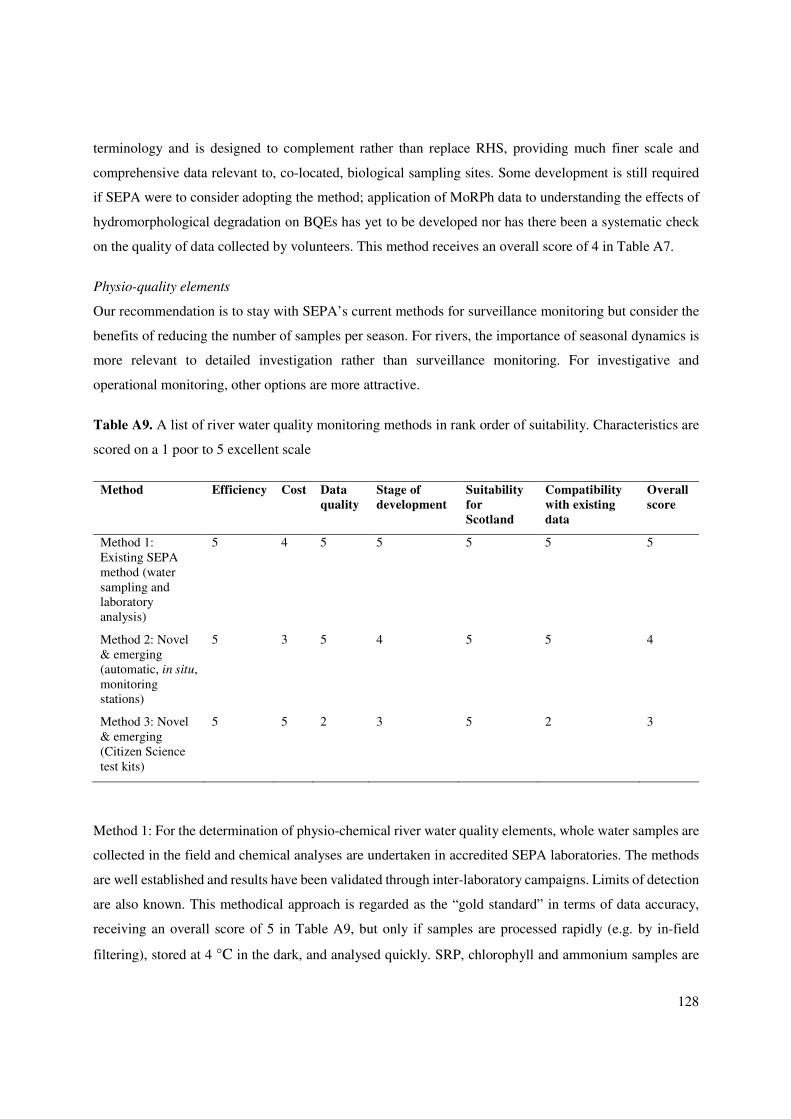
128
terminology and is designed to complement rather than replace RHS, providing much finer scale and
comprehensive data relevant to, co-located, biological sampling sites. Some development is still required
if SEPA were to consider adopting the method; application of MoRPh data to understanding the effects of
hydromorphological degradation on BQEs has yet to be developed nor has there been a systematic check
on the quality of data collected by volunteers. This method receives an overall score of 4 in Table A7.
Physio-quality elements
Our recommendation is to stay with SEPA’s current methods for surveillance monitoring but consider the
benefits of reducing the number of samples per season. For rivers, the importance of seasonal dynamics is
more relevant to detailed investigation rather than surveillance monitoring. For investigative and
operational monitoring, other options are more attractive.
Table A9. A list of river water quality monitoring methods in rank order of suitability. Characteristics are
scored on a 1 poor to 5 excellent scale
Method Efficiency Cost Data
quality
Stage of
development
Suitability
for
Scotland
Compatibility
with existing
data
Overall
score
Method 1:
Existing SEPA
method (water
sampling and
laboratory
analysis)
5 4 5 5 5 5 5
Method 2: Novel
& emerging
(automatic, in situ,
monitoring
stations)
5 3 5 4 5 5 4
Method 3: Novel
& emerging
(Citizen Science
test kits)
5 5 2 3 5 2 3
Method 1: For the determination of physio-chemical river water quality elements, whole water samples are
collected in the field and chemical analyses are undertaken in accredited SEPA laboratories. The methods
are well established and results have been validated through inter-laboratory campaigns. Limits of detection
are also known. This methodical approach is regarded as the “gold standard” in terms of data accuracy,
receiving an overall score of 5 in Table A9, but only if samples are processed rapidly (e.g. by in-field
filtering), stored at 4 °C in the dark, and analysed quickly. SRP, chlorophyll and ammonium samples are

129
particularly unstable, and ideally should be analysed within 24 hours of collection. Samples also need to be
taken at an appropriate frequency, to capture the rapid water quality dynamics. Monthly sampling (or three-
monthly, as the EA are currently undertaking at many sites) will not capture high-flow events. The impact
of sampling frequency on load estimation and nutrient signal is demonstrated in Bowes et al. (2009). See
Figure A2, below, for an example from the River Frome, Dorset.
Figure A2. Example of annual phosphorus concentration data at different sampling frequencies in the River
Frome, Dorset.
130
Method 2: Automatic, in situ, monitoring stations. Electronic probes for DO, pH, conductivity, water
temperature, ammonium, nitrate, turbidity and total chlorophyll are all well developed and routinely used
in EA investigations, Water Company monitoring and as part of academic research. There are also
commercially available phosphorus and nitrogen spectrophotometric auto-analysers that can produce
excellent quality data, if installed and maintained correctly. A review of the latest high-frequency
monitoring systems and how the data can be used is given in (Rode et al. 2016).
Examples of automated data vs laboratory ground-truthing samples are given for the River Thames
tributaries in (Halliday et al. 2014) and The Cut (Halliday et al. 2015).
This high-frequency data produced by automatic monitoring stations is an extremely valuable resource. It
can be used to identify the presence of intermittent pollution sources, for example, periodic failures of a
sewage treatment works (Bowes et al. 2012), and to develop an understanding of nutrient dynamics (Cohen
et al. 2013). It can also be used to determine nutrient pollution sources, using a combination of Hysteresis
and Load Apportionment Modelling (Bowes et al. 2015). High-frequency chlorophyll data, alongside
supporting physical and water quality data, can be used to identify thresholds for algal growth, leading to
an understanding of the timing, magnitude and duration of algal blooms (Bowes et al. 2016). These methods
receive an overall score of 4 in Table A9.
Method 3: Citizen Science test kits offers the opportunity to get wide spatial coverage of water quality
parameters, but quality of data is an issue. There are issues around the choice of sampling site (which could
reflect the “agenda” of the sampler); for instance, samples could be taken within the effluent stream of a
STW and processed as the concentration of the river as a whole. Samples can also be clustered around
locations that are perceived to be a pollution source. These test kits receive an overall score of 3 in Table
A9.
A widely used test kit is the Kyoritsu packtest range http://kyoritsu-
lab.co.jp/english/seihin/list/packtest/po4.html. These are used internationally by Earthwatch to monitor
phosphate and nitrate concentrations in waterbodies across the world. The six-monthly Thames Water Blitz
https://freshwaterwatch.thewaterhub.org/totally-thames-water-blitz results in approximately 700 samples
to be taken across the Thames catchment on a single day. The sampling day coincides with CEH’s Thames
Initiative monitoring schedule that allows the results from the test kits to be directly compared with
traditional laboratory analysis (see Figure A3). The phosphorus results from the test kits are robust, although
the results are given as coarse concentration categories (<0.02; 0.02-0.05; 0.05 – 0.1; 0.1 – 0.2; 0.2 – 0.5;

131
0.5 – 1 mg P l-1) that are of little use in academic research. The nitrate test kits are not as robust and less
reliable.
Figure A3. Comparison of water quality results from Thames Water Blitz and CEH Thames Initiative
monitoring.
Lochs
Biological Quality Elements (BQEs)
Phytoplankton
Methods for loch phytoplankton are reviewed in two parts as new methods for phytoplankton abundance
offer very different options compared with methods for phytoplankton composition. Current field and
laboratory methods for phytoplankton abundance, measured as chlorophyll-a (chl-a), are standardised
across Europe and reliable. We do, however, recommend a potentially more cost-effective alternative of

132
using a hand-held sensor (fluorometer) for measuring chl-a. Almost real-time chl-a products using satellite
Earth observation data will also soon be available and have the potential to dramatically expand the number
of lochs, and monitoring frequency, from current chl-a monitoring by SEPA. These products are, however,
currently only validated for larger lochs >10 km2 area, although data from higher resolution satellites may
soon be available for smaller lochs.
Current UK field and laboratory methods for phytoplankton composition using standard microscopy
methods are comparable across Europe and SEPA methods are inter-calibrated and reliable. Imaging flow
cytometry is a potentially more cost-effective option but would require a “training period” for learning taxa
identities and studies to ensure comparability of composition, biovolume and WFD metric results.
Phytoplankton abundance
Current field and laboratory methods for phytoplankton abundance across Europe all adopt a standard
approach, chl-a measured spectrophotometrically following an International Standard. Some countries
additionally use total biovolume from microscopy counts. The SEPA method and metric is, therefore,
comparable, reliable and inter-calibrated. We do, however, recommend a potentially more cost-effective
option of using a hand-held sensor (fluorometer) for measuring chl-a. Almost real-time chl-a products using
satellite Earth observation data will also soon be available and have the potential to dramatically expand
the number of lochs, and monitoring frequency, from current chl-a monitoring by SEPA. These products
are, however, currently only validated for larger lochs >10 km2 area, although data from higher resolution
satellites may soon be available for smaller lochs.
Table A10. A list of monitoring methods for loch phytoplankton abundance in rank order of suitability.
Characteristics are scored on a 1 poor to 5 excellent scale.
Method Efficiency Cost Data
quality
Stage of
development
Suitability
for
Scotland
Compatibility
with existing
data
Overall
score
Method 1:
Existing SEPA
(Chl-a Spec.
method)
4 4 4 5 5 5 4.5
Method 2: Novel
& emerging (hand-
held sensor
(fluorometer))
5 5 5 5 5 5 5
Method 3: Novel
& emerging (Earth
observation)
5 5 4 4 4 5 4

133
Method 1: Determination of chlorophyll-a using spectrophotometric method. ISO standard available and
recommended for use. Efficiency and cost rated quite high, as most of cost is staff costs in visiting site.
Data quality is rated 4 as inter-laboratory differences can be quite large and samples can be affected by
contamination or poor storage. This existing SEPA method receives an overall score of 4.5 in Table A10.
Method 2: A novel and emerging method is the use of hand-held sensors (fluorometers). In vivo fluorometry
is the direct measurement of the fluorescence of chlorophyll in living algal cells, using a fluorometer.
Examples of fluorometers include: UniLux from Chelsea Instruments (approx. £2000) and the BBE
algaetorch (approx. £7000). A study by Pires (2010) reviewed 16 fluorometers from nine manufacturers in
terms of cost and ease of use for field purposes. It did not review reliability and detection limit. These
systems are generally reliable for chl-a, but can have problems with other algal groups due to similarities
in fluorescence between algal groups. The systems have a high capital cost (and maintenance cost) but
measurement in the field is quick and easy and requires no laboratory analysis. Several of the cheap hand-
held sensors can measures chl-a and Phycocyanin (cyanobacteria abundance) (that is 2 of 3 WFD
phytoplankton sub-elements). This novel and emerging method receives an overall score of 5 in Table A10.
Method 3: Another novel and emerging method for assessing loch phytoplankton abundance is Earth
observation. Tyler et al. (2016) review suitable satellite algorithms and products that are under development
for WFD monitoring. The approach is potentially very efficient and cost-effective at monitoring large
Scottish lochs, but currently not applicable to many WFD monitored sites which are smaller than the current
recommended applicable size (approx. >10 km2 but smaller possible dependent on basin shape). An
automated monitoring system is being developed in the NERC GloboLakes and EU EOMORES projects
using MERIS and Sentinel 3 satellite data (300 m resolution) and should be operational in the near future
to increase the frequency of monitoring of large Scottish lochs routinely. The use of higher spatial resolution
(10-60 m) data from Sentinel 2 would allow smaller lochs to be monitored. A new operational algorithm
selection procedure developed by the Universities of Stirling & Glasgow and PML provides a step-change
for surveillance monitoring as it allows automated selection of the optimal chl.-a retrieval algorithms to
apply to a broad range of loch types using MERIS & Sentinel data (Spyrakos et al. 2017). Further validation
of Sentinel 2 data products, especially for humic and low productivity Scottish loch types, would be
advisable. These Earth observation methods receive an overall score of 4 in Table A10.

134
Phytoplankton composition
Current SEPA field and laboratory methods for phytoplankton composition using standard microscopy
methods are inter-calibrated and reliable. Other inter-calibrated methods across Europe are very comparable
in approach and metrics used (Carvalho et al. 2013; Poikane et al. 2015). Imaging flow cytometry is a
potentially more cost-effective option but would require a “training period” for learning taxa identities and
validation studies to ensure comparability of composition, biovolume and metric results with existing inter-
calibrated methods.
Table A11. A list of monitoring methods for loch phytoplankton composition in rank order of suitability.
Characteristics are scored on a 1 poor to 5 excellent scale.
Method Efficiency Cost Data
quality
Stage of
development
Suitability
for
Scotland
Compatibility
with existing
data
Overall
score
Method 1:
Existing SEPA
method
(microscopy)
3 3 4 5 5 5 4
Method 2: Novel
& emerging
(imaging
cytometry
4 3 4 4 5 5 4
Method 3: Novel
& emerging (flow
cytometry
5 3 2 4 2 1 2
Method 4: Novel
& emerging
(molecular
approaches
(eDNA)))
4 3 1 2 4 1 2
Method 5: Novel
& emerging (hand-
held sensor
(fluorometer))
5 3 1 5 5 1 1
Method 1: Determination of phytoplankton composition is carried out using the Utermohl technique
(manual identification and counting using inverted microscope). CEN standards exist for the routine
analysis of phytoplankton abundance and composition (CEN 2004; CEN 2008) and UK (and SEPA)
guidance (WFD-UKTAG 2014f) is based on this. Efficiency and cost are rated average, as there are staff
costs in visiting site and specialist analysis at the microscope. Data quality is rated 4 as inter-laboratory

135
(analyst) differences are apparent and samples can be affected by contamination or poor storage. This
existing SEPA method receives an overall score of 4 in Table A11.
Method 2: Imaging flow cytometry (IFC) is a hybrid technology combining the speed and large sample size
capabilities of flow cytometry with conventional imaging capabilities of microscopy. The approach is more
routinely used in “cleaner” marine phytoplankton studies, as it is potentially much more cost-efficient than
routine microscopy, is less biased and less prone to counter identification error (Dashkova et al., 2017). It
also captures smaller pico-plankton more effectively. Its main disadvantage over existing conventional
microscopy is that it would require a manual training period with some overlap with manual microscopy
identification to ensure taxa common in Scottish waters are correctly identified by the machine learning
algorithms. Due to the limitations of automated identification it also generally has less taxonomic resolution
and greater errors are reported from species-rich phytoplankton samples from natural waters, particularly
when more structurally complex colonial or filamentous taxa are present (Jakobsen and Carstensen 2011;
Dashkova et al. 2017). Adoption of this technology would, therefore, require careful comparison to ensure
it provided comparable data to existing inter-calibrated methods. In summary, it has the clear potential to
be more cost-effective than current methods, but its potential for analysing freshwater phytoplankton
composition from Scottish waters is currently untested. This method receives an overall score of 4 in Table
A11.
Method 3. Flow cytometry is a well-established tool for phytoplankton community analysis, with
advantages of rapid, high-throughput analysis and size and fluorescence measurements that allow some
discrimination of community composition (e.g. Read et al. 2014). In spite of these advantages, it is not
suitable for replacing conventional microscopy approaches for WFD assessment, mainly due to the lack of
taxonomic resolution that it provides (Dashkova et al. 2017); taxa can only be distinguished at the class
level at best. The emerging technology of imaging flow cytometry (IFC) (Method 2) offers much greater
potential for WFD monitoring purposes. This method receives an overall score of 4 in Table A11.
Method 4: There is clear potential in developing metabarcoding molecular approaches using whole
community analysis of integrated water column or outflow samples. Current activities on metabarcoding
approaches in Europe, such as DNAquanet, have not, however, focused on developing DNA libraries of
common phytoplankton species, so currently the methods are not close to readiness. For these reasons, this
method scores low for data quality, stage of development and comparability with existing data (Table A11).
SEPA should maintain a watching brief. These approaches would also not provide the actual abundance of
taxa and so are not comparable with existing inter-calibrated metrics. Future inter-calibration comparison
136
of new metrics based on presence/absence or relative abundance would, therefore, be required. These
molecular approaches receive an overall score of 2 in Table A11.
Method 5: Another novel and emerging method is the use of hand-held sensors (fluorometers), for example,
the BBE fluoroprobe (approx. £20,000). A study by Pires (2010) reviewed 16 fluorometers from nine
manufacturers in terms of cost and ease of use for field purposes. It did not review reliability and detection
limit. From experience, these systems are generally unreliable for distinguishing all algal classes due to
similarities in fluorescence between certain algal groups (e.g. overlap between diatoms and dinoflagellates).
Cyanobacteria are generally well resolved. Measurement in the field is quick and easy and requires no
laboratory analysis but they provide insufficient taxonomic resolution for WFD classification purposes. For
these reasons, this method scores very low for data quality and comparability with existing data in Table
A11. They also have a high capital and maintenance cost. Therefore, this method receives an overall score
of 1 in Table A11.
Macrophytes & phytobenthos
Macrophytes
The current SEPA method, Lake LEAFPACS2, receives the highest overall score of all the evaluated loch
macrophyte monitoring methods. This inter-calibrated method has undergone a considerable period of
development, and is well designed for Scottish standing waters and produces high quality, reliable data
suitable for WFD purposes and is relatively efficient and cost-effective. Current SEPA field surveys remain
the most suitable method to deliver WFD requirements on composition and abundance. Other alternative
inter-calibrated and novel approaches, such as the use of macrophyte maximum colonisation depth
measurements and hydroacoustics, can provide useful supplementary information on macrophyte coverage
and abundance in lochs but still need to be combined with more ‘traditional’ point-intercept methods to
accurately assess macrophyte community composition. Further development of metrics sensitive to hydro-
morphological pressures could be developed, as in Finland, but would require elaboration of field survey
methods to include emergent communities. Other novel and emerging methodologies, such as satellite
remote sensing, although potentially valuable for extending the spatial and temporal monitoring coverage
of lochs, cannot yet provide the detailed assessments, particularly of submerged plants, for accurately
assessing loch macrophyte communities. Molecular approaches are also not currently well developed
enough to assess macrophyte communities in Scottish lochs.

137
Table A12. A list of monitoring methods for loch macrophytes in rank order of suitability. Characteristics
are scored on a 1 poor to 5 excellent scale.
Method Efficiency Cost Data
quality
Stage of
development
Suitability
for
Scotland
Compatibility
with existing
data
Overall
score
Method 1: Existing
SEPA (Lake
LEAFPACS2)
3 3 5 5 5 5 4.5
Method 2: Novel &
emerging
(hydroacoustics)
5 4 3 5 4 4 4
Method 3:
Alternative inter-
calibrated method
(e.g. Macrophyte
Maximum
Colonisation Depth)
4 4 3 4 4 4 4
Method 4: Novel &
emerging (remote
sensing)
5 4 2 3 3 3 3.5
Method 5: Novel &
emerging (molecular
approaches)
5 5 2 2 5 2 3
Method 1: The current SEPA WFD loch macrophyte assessment method is Lake LEAFPACS2 (WFD-
UKTAG 2014e) LEAFPACS2 forms one part of the WFD quality element “macrophytes and
phytobenthos”. It is primarily designed to detect the impact of nutrient enrichment on UK lake macrophyte
communities although it may also be sensitive to other pressures or combination of pressures, for example,
shore modification (WFD-UKTAG 2014e). The loch macrophyte metrics derived from this method are
calculated using field survey data collected in the summer months using a standardised series of transects
in a sector sampling approach that conforms to the CEN 15460: 2007 Water quality – guidance standard
for surveying of macrophytes in lakes (CEN 2007). Efficiency and cost are rated 3 in Table A12 as the
method is labour intensive requiring a minimum of two staff from SEPA’s National Monitoring Team to
carry out each loch macrophyte survey. Ideally, lochs are surveyed annually but it in practice a survey once
every six years is regarded as a satisfactory frequency for assessing a loch’s macrophyte community.
Species level identification of macrophytes requires a reasonably high degree of expertise and, hence,
training, but it can largely be done in the field. Other suitability criteria all score 5 in Table A12 as the
method as had long development and the data produced by it is considered reliable and compatible with

138
pre-existing Scottish datasets. The Lake LEAFPACS2 method receives an overall score of 4.5 in Table
A12.
Method 2: The use of hydroacoustic techniques has been used for some time to rapidly produce accurate
distribution maps of lake macrophytes and associated bathymetry (e.g. Valley et al. 2005; Winfield et al.
2007b). Using such techniques, the percent lake volume inhabited by macrophytes along survey transects
can be calculated and utilised to provide a rapid assessment of the apparent macrophyte maximum
colonisation depth (MCD) in lakes, which can be followed up, if necessary, by a more detailed examination
around this point, using traditional sampling methods, e.g. double-headed rake, to determine the actual
MCD (Spears et al. 2009). Such hydroacoustic methods can also provide high frequency estimates of
percentage volume inhabited (PVI) by which distinct macrophyte community colonisation versus depth
relationships can be observed (Spears et al. 2009). As the method is non-destructive, it allows repeatable
measures across the same transects annually, or as frequently as needed, allowing unbiased long-term trends
in cover, volume-inhabited and maximum growing depth to be reliably recorded. With the recent
development of new tools to automate the processing and creation of aquatic habitat maps using “off the
shelf” echo-sounder systems with internal GPS and cloud-based software, hydroacoustic methods can now
be used to help produce high frequency spatially referenced cover maps of macrophytes present in lakes.
For example, the BioBase system (Navico 2014) can be used to produce bathymetries and assessments of
the macrophyte communities and bottom characteristics of lakes using hydroacoustic data files recorded by
the echosounders. Given their portability, low cost and ability to be effective in relatively shallow water
opens up opportunities for such hydroacoustic systems to be more widely used (e.g. Citizen Science projects
using privately-owned boats) to collect repeatable, spatially-referenced macrophyte data in lakes. However,
hydroacoustics alone is not a suitable method to deploy if information on species composition of lake
macrophytes is required and needs to be combined with other ‘traditional’ point-intercept survey methods
to accurately assess macrophyte species abundance patterns and community composition in lakes (e.g.
(Valley et al. 2015). Hydroacoustic techniques receive an overall score of 4 in Table A12.
Method 3. Many EU countries have tried to develop WFD compliant lake macrophyte assessment methods,
of which 17 have been successfully inter-calibrated (Poikane et al. 2015). Nearly all the macrophyte
assessment methods (including LEAFPACS2) include sensitivity/tolerance metrics based on species
indicators values, e.g. trophic indices, or relative abundance of sensitive or tolerant taxa. Most of the inter-
calibrated lake macrophyte assessment systems also include some measure of abundance, usually maximum
macrophyte colonisation depth (though this is not included in LEAFPACS 2) and the abundance of
submerged macrophytes (Poikane et al. 2015). Macrophyte Maximum Colonisation Depth (Macrophyte
MCD) can be used as a proxy measure of macrophyte abundance in deeper lakes and is widely recognised

139
as being sensitive to anthropogenic pressures such as eutrophication, water level fluctuations and climate
change, as well as providing a direct measure of lake management activities, for example, if there is a shift
from a macrophyte dominated lake to a phytoplankton dominated one. Macrophyte metrics sensitive to
hydro-morphological pressures have been developed in Europe, e.g. Finland, and could be highly relevant
to Scottish lochs (Hellsten and Riihimäki 1996). Their implementation would, however, require elaboration
of field survey methods to include emergent communities. Alternative inter-calibrated methods receive an
overall score of 4 in Table A12.
Method 4: High resolution aerial images of lakes, taken with unmanned drones, allows for the identification,
mapping and abundance estimates of non-submerged macrophyte species, e.g. floating and emergent
vegetation. Satellite remote sensing also potentially allows for high spatial and temporal coverage with
consistency in measurement but normally cannot resolve species within mixed emergent vegetation stands
effectively or resolve species identification satisfactorily. Such remote sensing techniques receive an overall
score of 3.5 in Table A12.
Method 5: As for rivers, molecular approaches are not currently well developed for lake macrophytes and,
where attempted, it has not been possible to identify all the macrophyte species. Hence, for these reasons,
this method scores only 2 for data quality, stage of development and computability with existing data in the
suitability criteria (Table A12). However, in terms of efficiency, cost and suitability for Scotland, these
molecular approaches all score 5 in Table A12. If the methodological problems can be overcome, eDNA
could potentially be a very useful tool for monitoring invasive non-native plant species in lakes, particularly
for those submerged species that are easily missed or misidentified using traditional monitoring methods,
although it may be of limited use in detecting hybrids (Herder et al., 2014). Molecular approaches receive
an overall score of 3 in Table A12.
Phytobenthos
Current SEPA field and laboratory methods for loch phytobenthos using standard microscopy methods are
inter-calibrated and reliable. However, national WFD lake phytobenthos assessment methods, such as Lake
DARLEQ2, rely on determining the composition and relative abundance of diatoms, a process that requires
time-consuming species-level identification and a high degree of staff taxonomic expertise. New
metabarcoding approaches are potentially a more cost-effective option but require further development to
ensure all common taxa are identifiable and comparability with WFD metric results.

140
Table A13. A list of monitoring methods for loch phytobenthos in rank order of suitability. Characteristics
are scored on a 1 poor to 5 excellent scale.
Method Efficiency Cost Data
quality
Stage of
development
Suitability
for
Scotland
Compatibility
with existing
data
Overall
score
Method 1:
Existing SEPA
(Lake
DARLEQ2)
3 3 4 5 5 5 4.25
Method 2: Novel
& emerging
(molecular
approaches)
5 5 4 4 5 5 4.5
Method 1: Lake DARLEQ2 (Diatoms for Assessing River and Lake Ecological Quality) forms the
phytobenthos part of SEPA’s current WFD compliant method for assessing “macrophytes and
phytobenthos” in lochs and focuses on the benthic diatom assemblage composition, based on using the
Trophic Diatom Index (TDI) metric (WFD-UKTAG 2014g). The DARLEQ2 classification method is
designed to primarily detect nutrient enrichment pressures. It is based on the expert-derived riverine TDI
metric that was re-calibrated and applied to lake diatom communities (Bennion et al. 2014).
There are similar uncertainties associated with the Lake DARLEQ WFD method, as outlined earlier for the
equivalent River DARLEQ WFD method, so data quality gets a rating of 4 in Table A13. Efficiency and
cost is rated at 3 in Table A13 as species-level identifications are time consuming and require a high degree
of expertise and training. The Lake DARLEQ2 method receives an overall score of 4.25 in Table A13.
Method 2: As for rivers, new molecular approaches such as metabarcoding have been developed to provide
more cost-effective monitoring of lake diatom communities, compared with conventional methods that
require time consuming species level identification and a high degree of staff expertise. Such methods are
ready to be deployed by the EA as part of their routine freshwater monitoring programme in 2018 and
SEPA are investing in developing in-house capacity in new eDNA techniques for analysing diatom samples.
However, species-level assignment of sequences is hindered by a lack of fully populated reference
databases of barcodes. Metabarcoding can, however, describe diatom biodiversity to a higher resolution
than is usually possible by traditional morphometric methods. Molecular approaches receive an overall
score of 4.5 in Table A13.

141
Benthic invertebrates
The current main SEPA benthic invertebrate surveillance methods, CPET and LAMM, receive the highest
scores as they have undergone a lot of development, are well designed and produce high quality, reliable
data suitable for surveillance monitoring of the main stressors of nutrient enrichment and acidification
prevalent in Scottish lochs. Alternative inter-calibrated approaches, such as species richness/diversity
metrics and harmonized multimetric ecological assessment tools, also have the potential to be useful
additional techniques for assessing other anthropogenic pressures, such as morphological alterations, but
would require some development for use in Scotland and would still require labour-intensive sampling and
identification of collected samples. In contrast, molecular approaches score highly in terms of efficiency
and cost but still require some development work before they will be ready for deployment in Scottish
lochs.
Method 1: SEPA currently use two WFD lake methods for assessing the condition of the benthic
invertebrate fauna in lochs one of which is the Chironomid Pupal Exuviae Technique (CPET) (WFD-
UKTAG 2008a). The CPET metric is designed to be indicative of the impact of nutrient enrichment on the
benthic invertebrate biological quality element in UK lakes. The CPET metric is based on the composition
of chironomid species or group of chironomid species pupal exuviae collected from lake leeward shores in
four monthly samples (two hundred chironomid pupal exuviae in each sample) between April and October.
A CPET EQR is calculated based on observed and reference chironomid score values, resulting in an overall
EQR representing an ecological status class, as defined by the WFD, ranging from 0 (bad) to 1 (high). As
method requires the collection of four monthly samples and requires some taxonomic expertise to identify
chironomid pupal exuviae efficiency and cost were rated 4 but all the other criteria were rated 5 to give an
overall score of 4.5 in Table A14.

142
Table A14. A list of monitoring methods for loch benthic invertebrates in rank order of suitability.
Characteristics are scored on a 1 poor to 5 excellent scale.
Method Efficiency Cost Data
quality
Stage of
development
Suitability
for
Scotland
Compatibility
with existing
data
Overall
score
Method 1:
Existing SEPA
(CPET)
4 4 5 5 5 5 4.5
Method 2:
Existing SEPA
(LAMM)
4 4 4 5 5 5 4.5
Method 3:
Alternative inter-
calibrated (species
richness/diversity
metrics)
4 4 3 3 4 4 4
Method 4:
Alternative inter-
calibrated
(Harmonized
Multimetric
Ecological
Assessment
approach)
4 4 3 3 4 4 4
Method 5: Novel
& emerging
(molecular
approaches)
5 5 4 4 4 4 4
Method 2: The Lake Acidification Macroinvertebrate Metric (LAMM) is the second WFD compatible
method that SEPA use for assessing the condition of the benthic invertebrate fauna of Scottish lochs (WFD-
UKTAG 2008b). The LAMM is designed to detect the impact of acidification in UK lakes, based on the
benthic invertebrate community. LAMM can be used in lakes that are acid sensitive or in lakes that naturally
have a pH lower than 7. Benthic invertebrate samples are collected in the spring, using standardised
sampling protocols, from stony-bottomed areas in the shallow littoral of lakes. Method requires only one
sample to be collected and analysed in the spring so scores 4 for efficiency and cost in Table A14 but
method very specifically targeted for assessing sites sensitive to acidification and thus is not an appropriate
monitoring method for all lochs in Scotland. This method is given an overall rating of 4.5 in Table A14.
Method 3: Thirteen methods for the lake assessment of benthic invertebrates were successfully inter-
calibrated (Poikane et al. 2015) despite macroinvertebrates being considered as one of the most difficult

143
biological groups for assessing lake quality because of their complex biotic structure, and high spatial and
temporal variability (Solimini et al. 2006; Solimini and Sandin 2012). Sensitivity/tolerance metrics were
included in all the national systems reviewed in the inter-calibration exercise. These encompassed a range
of traditional indices, e.g. ASPT, as well newly developed sensitivity indices, e.g. the LAMM index. Eight
inter-calibrated methods also utilised species richness/diversity metrics, e.g. EPT (Ephemeroptera,
Plecoptera and Trichoptera) taxa richness, while only four methods contained composition metrics and
functional metrics were hardly used (Poikane et al. 2015). However, despite the development of all these
lake benthic invertebrate assessment systems, it is recognised that there still is a need to reduce the large
uncertainty in the metrics used to explain the relationship between lake benthos responses and
anthropogenic pressures (Poikane et al. 2015). These alternative inter-calibrated approaches are given an
overall rating of 4 in Table A14.
Method 4: Another alternative inter-calibrated method is the new harmonized multimetric ecological
assessment approach developed by Miler et al. (2013) using benthic invertebrates in relation to a specific
stressor in European lakes, in this case, morphological alterations of lake shores. Two biotic multimetric
indices were developed based on habitat-specific samples (Littoral Invertebrate based on HAbitat samples,
LIMHA) and composite samples (Littoral Invertebrate Multimetric based on Composite samples, LIMCO)
which were then correlated with a morphological stressor index to assess the ecological effects of
anthropogenic morphological alterations in a range of natural to heavily morphologically degraded lake
shores across a number of different geographical regions in Europe. Such stressor-specific assessment tools
could allow comparable lake morphology assessments to be made across Europe, as well as complying with
WFD standards, and could complement existing benthic invertebrate assessment approaches that are
primarily focussed on assessing the impact of lake eutrophication pressures. This alternative inter-calibrated
method is given an overall rating of 4 in Table A14.
Method 5: Bista et al. (2017) used a molecular approach by analysing an annual time series of lake eDNA
samples in order to describe temporal shifts in the Chironomidae community of a lake in the UK. They
were also able to show good correspondence between diversity estimates for this ecologically important
group using a variety of sampling techniques and concluded that eDNA metabarcoding can track seasonal
diversity at the ecosystem scale. There have also been a number of studies that have used DNA-based
methods to monitor macroinvertebrate invasive non-native species in lakes (e.g. Dougherty et al. 2016).
This molecular approach is given an overall rating of 4 in Table A14.

144
Fish
Compared with more conventional fish population assessment methods (e.g. gill netting), molecular
approaches, such as eDNA metabarcoding, appear to provide SEPA with the most cost-effective means of
monitoring lake fish populations. These molecular techniques have been validated for UK fish and are ready
for deployment, although there remain questions over estimating fish species abundances. These molecular
approaches receive the highest overall score of the evaluated river fish faunal methods. However, novel
hydroacoustic techniques are also sufficiently well developed to provide cost-effective, quantitative and
non-destructive means of rapidly getting data on fish abundance and distribution within lakes but need to
be supplemented by ‘traditional’ survey methods in order to identify fish species of interest.
Method 1: There are a number of Common Standard Monitoring techniques (e.g. gill netting and
hydroacoustics) that are employed for monitoring lake inhabiting fish species of conservation interest, for
example, Arctic Charr, whitefish and Vendace (JNCC 2015) but these are not designed for assessing whole
lake fish communities and are not carried out by SEPA staff.
Table A15. A list of monitoring methods for loch fish in rank order of suitability. Characteristics are scored
on a 1 poor to 5 excellent scale.
Method Efficiency Cost Data
quality
Stage of
development
Suitability
for
Scotland
Compatibility
with existing
data
Overall
score
Method 1: No
existing SEPA
method
N/A N/A N/A N/A N/A N/A N/A
Method 2: Novel &
emerging (molecular
approaches),
5 5 4 5 5 5 4.5
Method 3: Novel &
emerging
(hydroacoustics)
5 4 3 4 5 4 4
Method 4:
Alternative inter-
calibrated (pressure
index based on
expert judgement)
3 3 3 3 3 3 3
Method 2: Molecular approaches, such as the analysis of eDNA has the potential to provide valuable
information regarding the presence and absence of fish species, as well as the composition of whole fish
communities. Sampling can be as simple as collecting 0.5-1.0 L water samples across a water body.

145
Hanfling et al. (2016) successfully used eDNA metabarcoding to monitor UK fish species in a number of
large UK lakes, describing both fish diversity and relative abundance. Hanfling et al. (2016) showed that
even for a large lake like Windermere, as few as 10-20 samples were sufficient to capture c. 90% of fish
species known to be present – results which were consistent with its known fish community composition,
as monitored by extensive netting and other sampling activities such as hydroacoustics. Moreover, the
application of the eDNA metabarcoding in Windermere was precise enough to detect the real differences
between the fish community composition of the lake’s two basins in relation to their different trophic status.
Hanfling et al. (2016) also found that fewer samples needed for smaller standing waters. Hanfling et al.
(2016) were also able to detect sequences of a wide range of non-fish species such as otters and aquatic
birds in Windermere. The adoption of such eDNA methodology could allow a significant increase in the
number and diversity of waterbodies that are monitored, enabling data on species range shifts to be collected
on a national scale (Read et al. 2017). However, estimating fish species abundance using eDNA
metabarcoding is regarded as being more problematic although Hanfling et al. (2016) did show that this
approach could produce relative abundance estimates of the fish community in a large lake in line with
results accrued from long-term monitoring using more traditional sampling techniques. These molecular
techniques also have the potential to be used for the monitoring of invasive non-native species of fish in
lakes. As already outlined in the river section of this report, fish species in UK have a complete reference
database of fish species barcodes established. Molecular approaches have been developed and validated for
sampling UK fish populations and are ready to be deployed. Hence, for these reasons, all the listed criteria
in Table A15 are given scores of 5 apart from data quality that is given a rating of 4 because of the perceived
problems with estimating fish species abundance using these molecular approaches. This method is given
an overall score of 4.5 in Table A15.
Method 3: Hydroacoustic techniques have been used in recent years to show the abundance and distribution
of fish in lakes (Jones et al. 2008; Winfield et al. 2007a) and recent technical advances have allowed
hydroacoustic data to be used to assess features such as lake bottom substrates that can be important fish
habitats, for example for spawning (Winfield et al. 2015). Advantages of hydroacoustic techniques are that
they are cost-effective, quantitative and non-destructive means of rapidly obtaining data on lake fish
abundance, demographics and geographical distribution (Winfield et al. 2009; Winfield et al. 2012;
Winfield et al. 2013). It is possible to combine hydroacoustic methods with limited biological surveys to
identify fish species. Hydroacoustic methods alone will not be able to determine age, condition or sex of
individual fish but can be used to complement more ‘traditional’ fish sampling techniques, such as gill
netting, used to assess the populations of fish species of particular interest, for example, Arctic Charr,
whitefish species and Vendace (JNCC 2015). Hydroacoustics are rated 5 for efficiency and applicability

146
and 4 for other criteria apart from data quality that is given a score of 3. This method is given an overall
score of 4 in Table A15.
Method 4: An example of an alternative inter-calibrated approach to assess lake fish communities is to use
a pressure index, based on expert judgement. Despite fish being regarded as sensitive indicators of
environmental stress, the fish community of lakes is an often overlooked aspect of lake monitoring. This is
reflected in that only five EU member states have successfully inter-calibrated lake fish fauna assessment
methods (Poikane et al. 2015). The problems in of using fish communities as indicators of environmental
stress are as follows: the diverse range of sampling methods used across Europe; the management of the
lakes, e.g. fishing practices, fish stocking, introduction of non-native species have a large impact on natural
fish populations; lakes are subject to multiple pressures, and fish indirectly integrate the effects of these on
lower trophic levels; high natural variability in fish metrics; fish are mobile and can avoid areas of
environmental stress. Hence, there are few significant relationships between fish metrics and specific
pressure indicators. One possible way to overcome this problem is to base assessment of pressure on expert
judgement; in Austria, Germany and Italy such a response was demonstrated for individual sites. In their
overall fish assessments, based on a comparison of all methods employed at a site, a combined pressure
index was derived in which all the common pressures were scored and summed up to create an overall
pressure index (Poikane et al. 2015). This type of approach is not likely to be of wide application in Scotland
as there will be a lack of suitable data for many lochs with which expert judgements can be made to relate
fish populations with an index of pressure. For this reason, this method is given an overall score of 3 in
Table A15.
Supporting elements
Hydromorphological quality elements
According to the WFD, the hydromorphological elements that support the biological elements for lochs
are:
1. Hydrological regime
a. Quantity and dynamics of water flow
b. Residence time
c. Connection to groundwater body
2. Morphological conditions
a. Variation in loch depth
b. Quantity, structure and substrate of the loch bed
c. Structure of the loch shore
In relation to this, CEN guidance (CEN 2011) indicates that comprehensive data on hydromorphological
condition contributes to its WFD status classification at high ecological status (HES), only. The
147
hydromorphological condition assessment required for good and moderate status is that sufficient to support
the WFD biological elements, only.
Methods for collecting these data and making these assessments are outlined below:
Hydrological regime
Method 1: In terms of assessing the hydrological regime of lochs in relation to the WFD, SEPA apply
environmental standards that are relevant to determining the likely impact that disturbances to the loch level
regime (e.g. from abstraction or impoundments) will have on loch ecology. These standards recommend
allowable ranges for loss of loch shore habitat (e.g. as a result of loch level drawdown). To determine the
likely extent of such changes, SEPA model natural (without abstractions) and influenced loch levels, and
assess the impacts of these using bathymetric data. Where these data are not available, SEPA use expert
judgement based on known drawdown ranges and/or abstraction rates to estimate changes in loch shore
habitat. Residence times are estimated by dividing the volume of the loch by the modelled average discharge
at the loch outflow. This is a very cost effective method that has been developed for Scottish lochs, but is
very dependent on the quality and relevance of data for any given site. As many of these data are not
available on a site specific basis for many lochs, data quality may not be as good for some lochs as others.
The method has been used within SEPA for some time, so outputs are compatible with existing data. For
these reasons, this method has been given an overall score of 4 in Table A16.
Method 2: Flushing rates or retention times for lochs can be estimated from catchment characteristsics, loch
size and shape, flow data and meteorological records. This has been demonstrated at the European scale
using the AGRI4CAST dataset (http://agri4cast.jrc.ec.europa.eu/DataPortal/Index.aspx?o=d) and
landcover datasets that are available from the Centre for Ecology & Hydrology
(https://www.ceh.ac.uk/services/land-cover-map-2015). The total amount of water coming into each
catchment each day can be calculated and combined with loch volume to derive flushing rates and retention
times. This method has been verified for lakes across Europe that have flow gauges on their outflows.
Although small in number (<100), a good correlation was obtained between modelled and gauged values.
Large scale modelling to assess hydrological regime provides a general overview, but not site specific
detail. This is because the resolution and accuracy of large-scale data are low at the site specific level and
so the method is less suitable for use in Scotland than Method 1. Because the data are readily available, the
costs are relatively low compared to more site specific methods – especially those that require collection of
site specific data. Because this approach has not been used in Scotland, compatibility with existing data

148
will be lower than for Method 1. For these reasons, this method has been given an overall score of 3 in
Table A16.
Method 3: The Irish EPA use a similar method to the above, but use the bathymetry or volume of the lake
combined with measured water levels and rates of inflow, where available. In other cases, flushing rates
and retention times are derived from rainfall and evapotranspiration data. This method re-uses site-specific
data collected for other purposes and, as such, its efficiency is high. It has intermediate cost because the
time taken to compile and analyse data from third party sources are likely to be significant. It is, however,
a well-developed approach that is not dissimilar to Method 1 and, as such, is probably suitable for use in
Scotland and relatively compatible with existing data. For these reasons, this method has been given an
overall score of 3 in Table A16.
Table A16. A list of methods for quantifying hydrological regime, ranked in order of suitability.
Characteristics of each method are scored form 1 (poor) to 5 (excellent).
Method Efficiency Cost Data
quality
Stage of
development
Suitability
for
Scotland
Compatibility
with existing
data
Overall
score
Method 1:
Existing SEPA
method
4 5 3 4 4 4 4
Method 2: Large-
scale modelling
4 5 3 4 3 3 3
Method 3:
Combination of
measured and
modelled data
5 4 4 4 4 4 4
Morphological conditions
Method 1: SEPA collect data for some of the elements listed above, mainly the structure of the loch shore
and the deepest point of the loch, following Loch Habitat Survey (LHS) methodology (SNIFFER,
2008a). Principal use of the LHS data is to feed into SEPA’s Loch MImAS tool (SNIFFER, 2008b), which

149
is used for WFD classification and regulatory assessments. This tool has been developed to meet SEPA’s
operational requirements, and for use in Scotland.
Lake MImAS looks at the extent to which a range of eco-geomorphic attributes are affected by the range
of human morphological modifications that are typically encountered on lochs. It does so using expert
judgment, built into the tool, of the likelihood of morphological damage arising and of the extent to which
this is likely to have an impact on biota (plants, insects, fish), in order to come up with an assessment of
WFD status for loch morphology. This also links to biological status. The assessment takes into
consideration loch sensitivity through the use of loch typologies.
As LHS data are widely used for assessing lake morphological conditions in other European countries
(Ciampittiello et al., 2017), and it is unlikely that SEPA will consider using any other method, Method 1 is
the only method that has been scored for suitability in relation to quantifying loch morphological conditions.
It scores highly on efficiency, cost, stage of development, suitability for Scotland and compatibility with
existing data so the method has been given an overall score of 5 in Table A17.
Table A17. Method for quantifying morphological conditions, ranked in order of suitability.
Characteristics of the method are scored from 1 (poor) to 5 (excellent).
Method Efficiency Cost Data
quality
Stage of
development
Suitability
for
Scotland
Compatibility
with existing
data
Overall
score
Method 1:
Existing SEPA
method (Lake-
MImAS)
5 5 4 5 5 5 5
Physio-chemical quality elements
Under physical and chemical elements supporting the biological elements, the WFD lists the following
elements as being important for monitoring compliance:
1. General physico-chemical elements
a. Transparency
b. Thermal conditions
c. Oxygen conditions
d. Salinity

150
e. Acidification status
f. Nutrient conditions
2. Specific pollutants
a. Priority substances being discharged into the waterbody
b. Other substances being discharged into the waterbody in significant quantities
Methods for the above are outlined and discussed, below:
General physico-chemical elements
Method 1. Transparency, thermal and oxygen conditions, and salinity are currently measured by SEPA
from a boat using either a Secchi disk (for transparency), or an appropriate electronic probe system (for
temperature, oxygen, salinity). Although the cost of the equipment is relatively low, deployment requires a
boat manned by two trained personnel to comply with health and safety requirements. Therefore, overall
costs are high. The method is, however, well developed, suitable for use in Scotland and compatible with
existing data. For these reasons, this approach has been given an overall score of 4 in Table A18.
Method 2. Similar measurements can be made from an in situ monitoring buoy that has been fitted with
appropriate sensors and a data capture system. A remotely accessible data download facility reduces the
need for frequent visits, as does the installation of solar panels to increase battery life and wiper mechanisms
to keep probes clean. Although the method is efficient, the data quality good, the approach is well developed
and suitable for Scotland, with backward compatibility of data, the cost of installation and maintenance of
these systems is very high. Therefore, this method has been given an overall score of 2 in Table A18.
Method 3. Measurements could be taken with a remotely controlled vehicle (RCV), such as a boat or
airborne drone, fitted with appropriate lightweight sensors and a data logging capacity. Efficiency of use is
high, because it avoids the need for using a boat and removes the health and safety issues associated with
this. However, these methods are unproven and currently still under development (e.g. see
http://intcatch.eu/index.php/about-intcatch; https://nimbus.unl.edu/projects/co-aerial-ecologist-robotic-
water-sampling-and-sensing-in-the-wild/). The compatibility of the data that they would collect with
existing data is unknown, because probes need to be miniaturised to address weight issues and this may
affect the quality of data that they can collect. Although these systems have great potential the technology
is not well developed or tested at present. Therefore, this method has been given an overall score of 2 in
Table A18.

151
Table A18. A list of methods for quantifying transparency, thermal conditions, salinity and oxygen
conditions, ranked in order of suitability. Characteristics of each method are scored from 1 (poor) to 5
(excellent).
Method Efficiency Cost Data
quality
Stage of
development
Suitability
for
Scotland
Compatibility
with existing
data
Overall
score
Method 1:
Existing SEPA
(e.g. measurement
from a boat)
5 3 5 5 5 5 4
Method 2 Novel
& emerging
(automatic, in
situ, measurement
from a monitoring
buoy)
5 1 5 5 5 5 2
Method 3: Novel
& emerging
(probes fitted to
RCV)
5 3 4 1 5 3 2
Specific pollutants
Method 1: For the determination of acidification status, and of concentrations of nutrients and specific
pollutants in lakes, whole water samples SEPA collect whole water samples in the field and chemical
analyses are undertaken in their accredited laboratories. The methods are well proven and results have been
validated through inter-laboratory comparisons. Limits of detection are also known. However, collection
of water samples requires a field visit, preferably using a boat. In some cases, especially where no boat is
available, samples are collected from the outflow instead which reduces sampling costs. In this case, it is
assumed that there is a close relationship between the chemistry of the loch and that of its outflow. Water
samples are usually collected at the same time as measurements of transparency, thermal conditions, salinity
and oxygen conditions are taken. This reduces sampling costs, to some extent. The method scores very

152
highly for all criteria apart from cost, which is mainly due to labour intensive fieldwork being required to
collect samples. For this reason, Method 1 has been given an overall score of 4 in Table A19.
Method 2: A range of electronic probes have recently become available for determining chemical
concentrations in the field. This is especially true for ammonium and nitrate. There are also commercially
available phosphorus and nitrogen spectrophotometric auto-analysers available that can produce excellent
quality data if installed and maintained correctly. Probes or autoanalysers can be permanently installed (e.g.
on a monitoring buoy); in this case, the data obtained have a much higher temporal resolution than
occasional grab sampling from a boat. Ground truthing suggests that the data collected are compatible with
those collected by the more traditional methods outline in Method 1 (Halliday et al., 2014; Halliday et al.,
2015). However, initial investment costs to establish a buoy and/or autosampling system may be high and
maintenance costs can be significant. Although the method scored very highly on most other criteria, it was
given a very low score in relation to cost. For this reason, Method 2 was given an overall score of 2 in Table
A19.
Method 3: Citizen Science provides the opportunity to obtain wide spatial coverage of some water quality
parameters (especially those that can be recorded using low cost probes, and some water chemistry values).
However, for many purposes, data quality can be a problem. Issues can include the choice of sampling site
(which might reflect the particular interests or “agenda” of the person sampling; for example, samples may
be clustered around locations that are perceived to have a pollution source. A widely used test kit is the
Kyoritsu packtest range http://kyoritsu-lab.co.jp/english/seihin/list/packtest/po4.html. These are used
internationally by Earthwatch to monitor phosphate and nitrate concentrations in waterbodies. The 6-
monthly Thames Water Blitz (https://freshwaterwatch.thewaterhub.org/totally-thames-water-blitz) uses
these and collects 700 samples from across the Thames catchment on a single day. This coincides with
CEH’s Thames Initiative monitoring schedule, which allows the results from the test kits to be directly
compared with those from traditional laboratory analysis. The phosphorus results from the test kits have
been found to be robust, although the results are given as very coarse concentration categories (i.e. <0.02;
0.02-0.05; 0.05-0.1; 0.1-0.2; 0.2-0.5; 0.5-1 mg P l-1) rather than as actual concentrations. For this reason,
the data collected will not be accurate enough for WFD monitoring. For nitrate, the test kits are less robust
and the results are less reliable. Due to low data quality and lack of compatibility with existing data this
approach has been given an overall score of 2 in Table A19.

153
Table A19. A list of methods for quantifying acidification status, nutrients and specific pollutants, ranked
in order of suitability. Characteristics of each method are scored from 1 (poor) to 5 (excellent).
Method Efficiency Cost Data
quality
Stage of
development
Suitability
for
Scotland
Compatibility
with existing
data
Overall
score
Method 1:
Existing SEPA
(water sampling +
laboratory
analysis)
5 5 5 5 5 5 5
Method 2: Novel
& emerging
(probes deployed
from a boat or
monitoring buoy)
5 3 5 3 5 5 4
Method 3: Novel
& emerging
(Citizen Science
test kits)
5 5 2 3 5 2 2

154
Appendix 5.2: Case studies in efficient cost-effective monitoring
Current SEPA river surveillance monitoring
The network is set up to be sampled at a minimum of once every six years although some parameters are
sampled more frequently, to provide a strong enough signal (diatoms) or because they are also part of the
operational network and may require additional sampling if they are on the Good / Moderate boundary.
In general, diatoms and invertebrates are sampled at the same locations and concurrently when sampling
year coincides for the two BQEs. Chemistry is sampled by a different team at different times but typically
at the same location or in close proximity. Macrophytes will typically be sampled at one site that overlaps
with the other BQEs but for sufficient sample robustness up to five additional locations may be included to
create a strong data signal for a water body. Fish data are usually collected by Fisheries Trusts/DSFB for
their own purposes and supplied by some to SEPA, this sampling is, on occasion, augmented by SEPA
sampling to fill gaps in the network.
SEPA maintain a National Monitoring Team that carries out routine operational monitoring. SEPA maintain
a team of c. 40 ecologists with c. 30 active in the field .They conduct much of the sentinel surveillance BQE
monitoring. Sampling is typically conducted by one staff member for invertebrates and diatoms with two
staff for macrophytes. Hydromorphology is monitored by a separate team, as is hydrology.
Time per sample is planned using a standard average time per activity; 0.63 family level invertebrate
identification, 1.9 days per species level identification, 0.63 day for diatom samples, 0.6 day for
macrophytes or less (two persons).
New DNA techniques are attractive to SEPA but they wish to see proven ability. They will decide soon on
developing in-house capacity. SEPA have already commissioned DNA analysis for diatom samples from
monitoring network (200 samples this year)
The current network is biased towards medium to large rivers and may not be full representative of all
stressor – type combinations, although the most common stressor combinations are probably present in
some numbers. The ability of a site to represent a reach is something SEPA has considered and clear criteria
are documented.

155
Lessons learned
Benthic invertebrate data is considered to be robust rarely giving an unexpected signal that is not
explainable. Diatoms are inherently more variable and thus require more sampling effort to provide a
consistent signal.
At the start of full WFD monitoring, diatoms and invertebrates were monitored at river surveillance sites
every year – twice per year, spring and autumn. Since then sampling frequency has varied with resources
and experience, now for example diatoms are monitored every second year that allows for a sample to be
integrated over the years, which is more reliable.
Sensitivity to pressures is formalised in SEPA with particular BQEs or metrics considered indicative
although it is felt this is not always diagnostic and typically requires further resourcing and sampling across
groups where a genuine impact needs to be remedied. Some consideration should be given to the
redundancy in sampling some groups where they are likely to be insensitive to pressures.
The sentinel network is used to some extent to provide evidence for not monitoring some types of rivers as
intensively as their frequency in the landscape might suggest. Oligotrophic upland rivers in the highlands
are an example. Sites are contained in the network for the purpose of demonstrating these sites are not
impacted.
Surveillance monitoring in Finland
Finland is similar to Scotland in having a very large number of lakes and rivers. The river network is
between 300-400 sites. Invertebrates and diatoms are sampled approximately every third year while
macrophytes are sampled about once every six years. Macrophytes are sampled at a sub-set of c. 150 sites.
Invertebrates are sampled for one season only, in autumn. Where possible samples for different BQEs are
collected at the same location or in adjacent locations to facilitate sampling.
Fish are monitored by another government agency and this work is still carried out ‘in-house’. All other
groups, water chemistry and hydromorphology are sampled by consultants and the data is passed to open
or password protected online databases.
Two years ago, Finland reduced its surveillance network by 20%. The majority of monitoring moved from
the state agency SYKE to consultants with additional monitoring carried out by industry as a requirement
of discharge licences. The consultants must be certified as having the correct skills before tenders can be
awarded. Quality control is not formally carried out, thereafter, by SYKE. Many of the consultants are ex-

156
SYKE staff. SYKE retains about 1.5 staff per BQE with specialist expertise and these are supplemented by
about 10-15 regional hydrobiologists.
Driving and walking are sufficient to access sites despite the large area of the country.
Surveillance monitoring in the Republic of Ireland
The Irish EPA maintain a 180-site surveillance network for WFD, sampling benthic invertebrates and
macrophytes once in three years and phytobenthos twice in three years. Samples are co-located.
Physiochemical parameters are sampled once a month for 12 months for one year in six. For rivers,
hydromorphology is recorded using the River Hydromorphology Assessment Technique (RHAT) or the
Morphological Quality Index (MQI). The area covered is about 7/8 that of Scotland and is less
geographically complex.
Invertebrate samples are collected once in summer. This is considered to be the time of year that the
assemblages are most sensitive to stress and impact most detectable. Samples are sorted and identified on
the river bank – taking 1-2.5 hrs. Phytobenthos and macrophytes are sampled in a manner comparable with
UK monitoring methods.
The EPA has 12 FTE ecologists, eight of which focus on fresh waters. The team has responsibility for
monitoring but is also responsible for River Basin Management Plans. Following a cost benefit analysis,
33% of monitoring was outsourced. Time savings are less than expected due to the need to quality control
data and samples and time spent on tendering. Movement to framework agreements may reduce the
administrative burden. Field teams often combine EPA staff and contractors to help supervise standards
and meet health and safety requirements. There are concerns regarding the ongoing ability of the contractors
to provide a quality service, as experienced skilled staff retire – an issue which is acknowledged in the UK
also.
The EPA have adopted the use of ruggedized tablets and electronic versions of data forms. These have had
mixed success and require refinement with staff objecting to the additional time required for their use in
the field (about 30 minutes per site) and the challenges of using them in adverse conditions.
As in other EU member states, the Irish EPA are beginning to consider refinements to their surveillance
network, to create a data source that can help diagnosis as well as report on system state. This process is
refined by an improving understanding of system stresses and responses. This process is being funded
through the EPA’s grant awarding system and has required substantial investment.

157
Appendix 5.3: Outcome of UKEOF Workshop, 7-8 November 2017
The United Kingdom Environment Observation Framework (UKEOF) held a workshop, on the 7-8
November 2017, to discuss the future of sentinel monitoring. Representatives from all the UK environment
agencies, Natural England and JNCC attended. At our request, the chair of ECOSTAT and a representative
from the Irish EPA also attended.
Presentations were give on the interim findings of the statistical analysis and some of the findings regarding
emerging methods and sampling strategy. Presentations were also given on the Irish monitoring networks
and developments in Europe regarding the sensitivity of BQEs to pressures across member states. This was
followed by an interactive workshop that focused on future approaches to the development of sentinel-type
monitoring networks and the potential to add value through collaboration. Discussions were broad and
wide-ranging; points raised of direct relevance to this review are addressed below:
Attendees reacted positively to the sentinel project statistical analysis. Natural Resources Wales (NRW) are
intending to carry out their own statistical analysis of the representativeness of their networks. EA are also
considering the possibility of doing something similar. It was revealed that only Germany collects more
samples than the UK for WFD reporting.
Attendees were interested in the emerging methods. The EA are already trialling an eDNA method for
diatoms and the project is progressing well. The EA suggested that there would be marginal savings in
using hand-held chlorophyll sensors compared with using traditional techniques. It was generally
acknowledged that new methods would need to provide data compatible with existing methods.
There was an acknowledgement by the chair of ECOSTAT that emerging technologies had potential and
he suggested that where application could be demonstrated and a consensus agreed among member states
that would generate the potential for change at an EU level.
There were few suggestions for specific questions that the agencies wanted answered by a surveillance
network other than the core business of tracking change through time. There was a general feeling that there
is potential within the networks and strategic questions could be formulated.
Better means of collaboration and information exchange were considered necessary during the forthcoming
period of change.


