
HAL Id: hal-02390432https://hal.archives-ouvertes.fr/hal-02390432
Submitted on 6 Dec 2019
HAL is a multi-disciplinary open accessarchive for the deposit and dissemination of sci-entific research documents, whether they are pub-lished or not. The documents may come fromteaching and research institutions in France orabroad, or from public or private research centers.
L’archive ouverte pluridisciplinaire HAL, estdestinée au dépôt et à la diffusion de documentsscientifiques de niveau recherche, publiés ou non,émanant des établissements d’enseignement et derecherche français ou étrangers, des laboratoirespublics ou privés.
Seismic history from in situ 36Cl cosmogenic nuclidedata on limestone fault scarps using Bayesian reversible
jump Markov chain Monte CarloJ. Tesson, Lucilla Benedetti, Jump Markov, Monte Carlo
To cite this version:J. Tesson, Lucilla Benedetti, Jump Markov, Monte Carlo. Seismic history from in situ 36Cl cos-mogenic nuclide data on limestone fault scarps using Bayesian reversible jump Markov chain MonteCarlo. Quaternary Geochronology, Elsevier, 2019, 52, pp.1-20. �10.1016/j.quageo.2019.02.004�. �hal-02390432�

1
2 Seismic history from in situ 36Cl cosmogenic nuclide data on 3 limestone fault scarps using Bayesian Reversible Jump Markov 4 chain Monte Carlo5 6 Tesson J.1 and Benedetti L.1
7 1 Aix-Marseille Université, CEREGE CNRS-IRD UMR 34, Aix en Provence, France
8 Corresponding author: J. Tesson, Aix-Marseille Université CEREGE CNRS-IRD UMR 34,
9 Plateau de l’Arbois, Aix en Provence, 13545, France. ([email protected])
1011
12 Abstract13 Constraining the past seismic activity and the slip-rates of faults over several millennials is
14 crucial for seismic hazard assessment. Chlorine 36 (36Cl) in situ produced cosmogenic nuclide
15 is increasingly used to retrieve past earthquakes histories on seismically exhumed limestone
16 normal fault-scarps. Here we present a new methodology to retrieve the exhumation history
17 based on a Bayesian transdimensional inversion of the 36Cl data and using the latest muon
18 production calculation method. This procedure uses the reversible jump Markov chains
19 Monte-Carlo algorithm (RJ-MCMC, Green 1995) which enables 1-exploring the parameter
20 space (number of events, age and slip of the events), 2-finding the most probable scenarios,
21 and 3- quantifying the associated uncertainties. Through a series of synthetic tests, the
22 algorithm revealed a great capacity to constrain event slips and ages in a short computational
23 time (several days) with a precision that can reach 0.1 ky and 0.5 m for the age and slip of
24 exhumation event, respectively. In addition, our study show that the amount of 36Cl
25 accumulated when the sampled fault-plane was still buried under the colluvial wedge, prior its
26 exhumation, might represents up to 35 % of the total 36Cl. Additional sampling under the
27 colluvial is necessary to constrain this contribution.
28 Introduction
29 Active normal faults in carbonated environments often produced continuous 1-20 m high
30 bedrock fault scarp as the result of one-to-several earthquake displacements on the fault
31 plane. This has been recently well illustrated during the 30/10/16 Amatrice earthquake of
32 Mw=6.5 that triggered an exhumation of 1 to 2 m of the base of the limestone fault scarp

33 along at least 7 km (see Fig. 1) (Villani et al. 2018, Perouse et al. 2018). When those
34 morphological features are preserved from natural and anthropogenic degradation, they
35 can be used as a marker of paleo-earthquakes allowing recovering crucial information
36 about the timing and the magnitude of the past large earthquakes. Few studies have
37 proposed to assess the amplitude of the past slip events using the morphology of the fault
38 plane surface. In particular, the presence of horizontal bands of lighter color on some fault
39 planes visible on aerial pictures and/or backscattered electromagnetic signals, or the brutal
40 end of vertical karstic weathering features (flutes) on some fault planes have suggested
41 that they might represent paleo–interface between the exhumed fault plane and the
42 colluvium soil, that have been uplifted because of earthquakes (Giaccio et al., 2012; Wiatr
43 et al., 2015). Recently, high-resolution digital elevation models of the exhumed fault plane
44 of the Pisia fault (Greece) revealed a vertical variability of the roughness along the fault
45 plane, with peaks delimiting deci-to-decametric horizontal bands (Wiatr et al., 2015; He et
46 al., 2016). Those studies thus suggest that the exhumation process producing the fault-
47 plane, or its exposure history since exhumation might be able to partially control its
48 physical properties. On the other hand, the systematic chemical analysis of the carbonated
49 bedrock fault plane along vertical profiles has revealed that the concentration of the in situ
50 produced cosmogenic nuclide 36-Chlorine (36Cl) and the concentration of the rare earth
51 elements (REE) are highly modulated by the exhumation process (Carcaillet et al., 2008).
52 The approach based on the measured content of in-situ produced 36Cl has provided an
53 unique opportunity to determine both the slip of the past large earthquakes, and to date
54 those events (Mitchell et al., 2001; Benedetti et al., 2002; Schlagenhauf et al., 2010). The
55 REE content analysis has improved our capacity to distinguish slip events because the
56 buildup kinematic appears to be faster than the 36Cl in situ production (Carcaillet et al.,
57 2008; Tesson et al., 2016).
58 At the same time, the thorough analysis of the fault-scarp geometry and of the colluvial
59 wedge sub-surface morphology by means of field observations and geophysical
60 investigations (Lidar, GPR) have proven to be essential to assess the origin of the fault
61 plane exhumation (Schlagenhauf et al., 2010; Giaccio et al., 2012; Bubeck et al., 2015;
62 Wilkinson et al., 2015). For instance, erosion of the fault scarp by collapsed of
63 unconsolidated portion of the scarp, fluvial erosion due to drainage crossing the fault or
64 anthropogenic modifications can modify the exhumation chronology, avoiding reliable
65 results on the seismic exhumation history.
66

67 So far, the only possibility to date the exhumation of a carbonated fault plane is to use the
68 36Cl cosmogenic nuclide which results from the interaction of cosmic rays and mainly the
69 Calcium contained in carbonate rocks. Determining the 36Cl concentration ([36Cl]) of rock
70 samples collected on a fault-plane surface thus potentially enables to date the different
71 exhumational phases of the fault plane and quantify the amplitude of each slip events
72 (Benedetti et al., 2002; Mitchell et al., 2001). Because cosmic rays are able to penetrate up
73 to 4-10 m depth below the ground surface (Gosse and Phillips, 2001; Schlagenhauf,
74 2010), a today-exhumed fault plane has firstly accumulated 36Cl at depth when buried
75 below the colluvium, and secondly when exhumed and directly exposed to cosmic rays
76 (Schlagenhauf et al., 2010). The exhumation age of a sample belonging to the fault plane
77 surface thus requires integrating its whole exhumation history from depth to surface, that
78 is modulated by the number of events, their displacements and ages. Several pioneering
79 studies applied the equations describing the cosmogenic production to such dynamic
80 surface providing a way to precisely calculate the vertical synthetic [36Cl] profile that
81 should be observed on a fault-plane for a given exhumation scenario (Mitchell et al.,
82 2001; Benedetti et al., 2002, 2003; Schlagenhauf et al., 2010). Over the last five years,
83 more than a dozen of seismic histories have been inferred from 36Cl cosmogenic dating of
84 seismically exhumed fault plane (Schlagenhauf et al., 2011; Akçar et al., 2012; Benedetti
85 et al., 2013; Mouslopoulou et al., 2014; Tesson et al., 2016; Cowie et al., 2017) all using
86 the latest published methodology (Schlagenhauf et al., 2010). More recently, Beck et al.
87 (2018) published a new modelling code, built upon the Schlagenhauf et al. (2010) code
88 with an inversion procedure. Here we present a new inversion procedure (called
89 Modelscarp inversion) using a Reversible Jump Markov chain Monte Carlo ( RJ-McMC,
90 Green, 1995; Gallagher et al., 2011; Sambridge, 2012), in which we include the full 36Cl
91 build-up of a fault scarp with in particular an updated muon production rate calculation.
92 We show through synthetic tests that our modelling is able to decipher with great accuracy
93 complex scenario including seismic clusters and quiescence periods, and that accounting
94 for the slip history prior to the post-glacial exhumation is crucial. The code and a
95 complete tutorial are released in the present article
96 (https://github.com/jimtesson/Modelscarp_Inversion).
979899 I. Recovering past earthquakes from a 36Cl profile

100 1. Formation and preservation of normal fault-scarp
101 Many authors attribute the persistence of limestone bedrock fault-scarp along normal
102 faults to be the direct consequence of climatic condition changes in the Mediterranean
103 that occurred at the end of the last glacial maximum period (Armijo et al., 1992;
104 Giraudi and Frezzotti, 1995; Piccardi et al., 1999). This major climatic change from
105 cold glacial to warmer inter-glacial conditions apparently resulted in an abrupt
106 decrease of the hill-slope erosion rate and a general stabilization of mountain slopes
107 by the vegetation as suggested by several records in continental lakes showing a
108 drastic decrease of clastic input and an increase of terrestrial vegetation (Giaccio et
109 al., 2015). This environmental modification has led to preserve the vertical offset
110 produced by normal faulting over the last 16-20 kyr (Armijo et al., 1992; Giraudi and
111 Frezzotti, 1997; Piccardi et al., 1999; Tucker et al., 2011). Hence, the 1-20 m high
112 steep scarp commonly observed along active normal faults (Fig. 2) have long been
113 interpreted as being the cumulative vertical offset caused by multiple co-seismic
114 displacement on the fault plane over the last 18 ka (hereinafter referred as the “post-
115 glacial” fault-scarp). Those preserved fault-scarps are usually topped by a relatively
116 smooth and gentle 10-40◦ dipping surface (hereinafter referred as the “peri-glacial
117 surface”, Fig 2), representing the older exhumed footwall, that has progressively
118 retreated from the fault plane due to the long-term abrasion that occurred during peri-
119 glacial period (Tucker et al., 2011). During those periods of enhanced erosion, a
120 significant amount of sediments is deposited on the hanging-wall compartment of the
121 fault, forming a colluvial wedge at the base of the fault plane (Fig. 2). Schlagenhauf
122 et al. (2011) dated with radiocarbon dating two charcoal found in the colluvial wedge
123 of the Magnola fault scarp at 31.6 ± 0.5 and 38.8 ± 1.2 ka BP. Those ages are in
124 agreement with the assumption that the colluvial wedge has been deposited during the
125 Pleistocene.
126
127
128 2. 36Cl build-up in an exhumed fault plane
129 (i) 36Cl accumulation in the fault-plane130131 The 36Cl accumulation within a rock sample belonging to a fault-plane have been
132 formalized by Schlagenhauf et al. (2010). The model includes various factors that
133 modulate the 36Cl production rate within the rock, such as the site location, the

134 shielding resulting from the geometry of the fault-scarp and associated colluvium, the
135 scarp denudation, the chemical composition of the fault-plane rock and of the
136 colluvial wedge, the geomagnetic field temporal variations, and the possible snow
137 cover.
138 Basically, in absence of denudation, the concentration of 36Cl in a rock varies as a
139 function of rock exposure time (t) and burial depth (z), as𝑑𝑁(𝑧,𝑡)/𝑑𝑡 = 𝑃36𝐶𝑙 (𝑧,𝑡) ‒ 𝜆 × 𝑁(𝑧,𝑡) Eq. (1)
140 where N is the number of atoms of 36Cl, P36Cl is the 36Cl isotope production rate, λ is
141 the decay constant of 36Cl, and dN /dt is the rate of change.
142 According to Schlagenhauf et al. 2010, the total 36 Cl production rate for a preserved
143 rock sample (i.e. sustaining no denudation) of a normal fault scarp, close to the
144 ground surface, can be calculated:
𝑃36𝐶𝑙 (z,t) = 𝑃(𝑧) × 𝑆 (𝑡) × 𝐹(𝑧) × 𝑄 + 𝑃𝑟𝑎𝑑 Eq. (2)
145
146 P(z) is the sample-specific 36Cl production rate modulated by the sample chemical
147 composition and the sample depth, and Prad is the radiogenic production. S, F and Q
148 are scaling factors: S accounts for elevation, latitude and geomagnetic field (may vary
149 over the time), F accounts for the corrections related to shielding effects (topographic,
150 geometric and cover shielding) and may varies with sample position along the fault-
151 plane, and Q accounts for the sample thickness.
152 As shown by the equation (2), the amount of 36Cl in a sample of the fault-plane is thus
153 controlled by its position z (exhumed or buried) along the fault-plane, and by the time.
154 The amount of 36Cl in a sample thus integrates its whole history of exhumation, i.e. its
155 successive positions zi over the time, and the time periods Ti during which the sample
156 has remained at each position zi. In fine, the successive positions zi are directly
157 controlled by the amplitude of each slip event, while the time periods Ti corresponds to
158 the inter-event time between two slip event. Determining the exhumation history of a
159 fault-plane from its 36Cl content means resolving the successive position Zi of each
160 sample over the time.
161
162 The amount of 36Cl accumulated in a today-exhumed fault plane can be presented as
163 the sum of two contributions: a first contribution corresponding to the amount of 36Cl
164 accumulated at depth when buried under the colluvium during the peri-glacial
165 periods (> 18 ka), hereinafter called the inherited contribution ( ), and 𝑁 36𝐶𝑙 𝑖𝑛ℎ𝑒𝑟𝑖𝑡𝑒𝑑
166 a second contribution that accounts for the 36Cl accumulated during the post-glacial
167 exhumation of the fault-plane ( ). The final amount of 36Cl within each 𝑁36𝐶𝑙 𝑃𝐺
168 sample (i) is thus the sum of those two contributions (Eq. 1):
169
𝑁36𝐶𝑙 𝑓𝑖𝑛𝑎𝑙(𝑖) = 𝑁 36𝐶𝑙 𝑖𝑛ℎ𝑒𝑟𝑖𝑡𝑒𝑑 (𝑖) + 𝑁36𝐶𝑙 𝑃𝐺(𝑖) Eq. (3)
170
171 The modeling of the 36Cl accumulated within the fault plane during those two distinct
172 periods is explained in the following section.
173
174 (ii) Inherited 36Cl contribution
175 The initial conditions for the model are driven by the rate at which a footwall sample
176 is approaching the surface. We assume two cases to model this rate.
177 In the first case the normal fault has been slipping for a long-time period (> 50-100
178 kyr), which is attested by a long-term morphology (i.e. 100-300 m high topographic
179 scarp, presence of facet spur, strong incised gullies, perched valley (such as the
180 Sparta fault in Greece or the Magnola fault in Italy ; Benedetti et al., (2002); Palumbo
181 et al., (2004)) (Fig. 3-A). The inherited contribution is parameterized by the term
182 “slip-rate of the fault”, further called “peri-glacial fault slip-rate” that directly
183 controls the successive position Zi of each sample over the time.
184
185 This 36Cl contribution is numerically resolved for each sample of the fault plane by
186 predicting the position zi(t) over the time (Eq. 4). Samples are artificially placed at
187 greater depth where the production rate of 36Cl is null, and progressively raise
188 towards the surface according to the peri-glacial fault slip-rate (SR), finally reaching
189 their position just before the post-glacial exhumation history starts. At each time step
190 dt (=100 yr), z(t) is moves upward according to the peri-glacial fault slip-rate:
191
𝑧(𝑡𝑖) = 𝑧(𝑡𝑖 ‒ 1) + 𝑆𝑅 ∗ 𝑑𝑡 Eq. (4)
192

193 The inherited 36Cl ( ) within each sample is computed as the integral of 𝑁 36𝐶𝑙 𝑖𝑛ℎ𝑒𝑟𝑖𝑡𝑒𝑑
194 the 36Cl accumulated over the duration of the inherited period:
𝑁 36𝐶𝑙 𝑖𝑛ℎ𝑒𝑟𝑖𝑡𝑒𝑑 =300 𝑘𝑦𝑟
∫0
𝑃36𝐶𝑙(𝑧(𝑡)) ×(1 ‒ 𝑒 ‒ 𝜆𝑑𝑡)
𝜆 Eq. (5)
195
196 where is the theoretical number of atoms of 36Cl accumulated in the 𝑁 36𝐶𝑙 𝑖𝑛ℎ𝑒𝑟𝑖𝑡𝑒𝑑 197 sample during the rise of the sample, P36Cl is the 36Cl production rate within each
198 sample depending on the depth of the sample z, λ is the decay constant of the 36Cl,
199 and t is the time since the fault started to slip. The duration of the long-term rise can
200 be evaluated from the height of the long-term topographical scarp at each site and
201 assuming an a priori peri-glacial slip-rate (Fig. 3-A). For instance, a cumulative fault
202 scarp of 300 m high produced by a fault slipping at 1 mm/yr would give a maximum
203 duration of 300 kyr.
204
205 In the second case, the fault has not been active in the past, or its slip-rate was very
206 low. The erosional processes mainly control the overall morphology of the scarp (Fig.
207 3-B), with no long-term topographical scarp and a low dipping peri-glacial abrasion
208 surface (<10o), as observed for example at the Nahef fault (Israel, Mitchell et al.,
209 (2001)), the Kaparelli fault (Benedetti et al., (2003), or the Fiamignano fault (Bubeck
210 et al. 2015)). In that case, the inherited 36Cl contribution is directly controlled by the
211 denudation rate, the surface is at steady state prior exhumation (Fig. 3-B). In such
212 case, the inherited 36Cl is also parameterized using Eq. 5, i.e. samples are artificially
213 placed at greater depth where the production rate of 36Cl is null, and progressively
214 raise towards the surface according to the long-term (or peri-glacial) denudation-rate
215 (ε). Since the 36Cl production originating from muons might be important at depth
216 (Balco, 2017; Braucher et al., 2011), the inherited contribution can account for a
217 significant proportion of the total measured 36Cl in the sample, and has to be
218 considered.
219
220
221
222 (iii) 36Cl contribution from Post-glacial exhumation (< 20 kyr ago)

223 When warmer conditions are renewed, the fault plane is progressively exhumed from
224 below the colluvium by successive earthquakes and preserved until today because of
225 low erosion-rate and low supply of sediments preventing the fault plane from being
226 dismantled or buried. Calculating the 36Cl build up on a sample from the fault plane
227 during the post-glacial period consists in resolving the successive positions z(t) of the
228 sample over time, which modulates the 36Cl production rate (see Eq. 2). After each
229 event n, the depth position of the sample is updated as a function of its position prior
230 to the event ( ), and the event displacement ( ):𝑧𝐸𝑣 𝑛 ‒ 1 𝑆𝑙𝑖𝑝𝐸𝑣 𝑛
𝑧𝐸𝑣 𝑛 = 𝑧𝐸𝑣 𝑛 ‒ 1 + 𝑆𝑙𝑖𝑝𝐸𝑣 𝑛 Eq. (6)
231
232 The 36Cl production rate is thus controlled by the displacement of each slip event that
233 directly modifies the depth position of the sample. The time period during which the
234 sample has remained at each position z and has accumulated 36Cl is controlled by the
235 time between each event.
236 In our model, the 36Cl accumulated during the post-glacial period is thus
237 parameterized by a given number of slip events, by their displacements, and by their
238 ages. Those parameters enable to calculate the successive position of a sample and
239 thus its 36Cl production rate over the time. The post-glacial 36Cl contribution is
240 computed within each sample as being the sum of the 36Cl accumulated between each
241 event (Eq. 7):
242
𝑁36𝐶𝑙 𝑃𝐺 =𝑛𝐸𝑄𝑚𝑎𝑥
∑𝑛 = 1
𝑃(𝑧𝐸𝑣 𝑛) ×(1 ‒ 𝑒 ‒ 𝜆 × 𝑇𝑛→𝑛 + 1)
𝜆Eq. (7)
243
244
245
246 Where N36ClPG is the theoretical number of atoms of 36Cl accumulated in the
247 sample during the post-glacial period, n is the index of each earthquake, nEQmax is the
248 total number of earthquakes that exhumed the sampled fault-plane, zev n is the sample
249 depth position of the sample along the fault-plane after the n event, is the 𝑃(𝑧𝐸𝑞 𝑛)
250 production rate within the sample for the given zev n position, and is the time 𝑇𝑛→𝑛 + 1
251 period between two successive events n and n+1,

252
253 The uppermost and older section of the fault plane is often less well preserved, with
254 diffusion-shape profile toward the peri-glacial abrasion surface. Large fractures,
255 pockets and plugged vegetation are usually observed suggesting significant bio-
256 karstic weathering (Giaccio et al., 2012, Bubeck et al. 2015). Typically, this section is
257 not sampled for cosmogenic dating purpose (see Fig. 4) because the erosion might
258 significantly affect the [36Cl] signal. There are no data associated with this portion to
259 constrain the exhumation of this upper and older portion, which however needs to be
260 considered in the modelling since a significant amount of 36Cl is accumulated at
261 depth. We thus also account for that amount in the model as summarized in Fig. 4.
262 The total amount of 36Cl accumulated in the sampled profile thus integrates : 1) the
263 long-term inherited contribution (left panel in the Fig. 4), and 2) the 36Cl accumulated
264 during the seismic exhumation that includes the 36Cl accumulated during the post-
265 glacial exhumation of the uppermost fault plane, usually not sampled, called in the
266 following the “post-glacial inheritance” (central panel in the Fig. 4), and the 36Cl
267 accumulated during the post-glacial exhumation on the sampled portion, called in the
268 following “post-glacial exhumation” (right panel in the Fig. 4).
269
270 3. Modeling 36Cl profile and recovering exhumation histories
271
272 (i) Bayesian inference
273 Inferring the exhumational history of a post-glacial fault-plane from its in-situ 36Cl
274 content, means resolving the most probable number of events that progressively
275 exhumed the fault-plane, their displacements and their ages. The use of Bayesian
276 inferences is particularly well suited to this problem since it allows constructing a
277 statistical model fitting the data, integrating a priori information on the parameters,
278 and summarizing the results of each parameters by a probability distribution.
279 Bayesian approaches have been successfully applied in cosmogenic geochronology
280 (Muzikar and Granger, 2006; Schimmelpfennig et al., 2011; Marrero et al., 2016;
281 Laloy et al. 2017) to date morphological surfaces, and in paleoseismology (e.g. Buck
282 and Bard, 2007; Hilley and Young, 2008) to reconcile radiocarbon ages.
283 Here, we perform a “transdimensional” inversion (Sambridge et al. 2012) with the
284 reversible jump Markov chains Monte-Carlo algorithm (RJ-MCMC, Green 1995)
285 that allows a variable number of parameters.
286 A Bayesian inference aims at quantifying the a posteriori probability distribution of
287 the model parameters, m, given the observed data, dobs, noted as . 𝑝(𝑚│𝑑𝑜𝑏𝑠)
288 Following Baye’s rule, the posterior distribution is deduced from the combination of
289 the model structure ) and the prior :𝑝(𝑑𝑜𝑏𝑠|𝑚) 𝑝(𝑚)
290
𝑝𝑜𝑠𝑡𝑒𝑟𝑖𝑜𝑟 ∝ 𝑙𝑖𝑘𝑒𝑙𝑖ℎ𝑜𝑜𝑑 × 𝑝𝑟𝑖𝑜𝑟 (8)
291
𝑝(𝑚│𝑑𝑜𝑏𝑠) ∝ 𝑝(𝑑𝑜𝑏𝑠|𝑚)𝑝(𝑚) (9)
292
293
294 where the likelihood function , is the probability that the model reproduces 𝑝(𝑑𝑜𝑏𝑠|𝑚)
295 the observed data given the model m. The prior is the probability of the set of 𝑝(𝑚)
296 parameters m, representing our knowledge of m before performing the inference.
297 The posterior distribution thus represents how our prior knowledge of parameters m is
298 able to reproduce data.
299 Posterior distributions are constructed by sampling the parameter space in such a way
300 that the sampling density of each parameter reflects that of the posterior distribution.
301 In order to infer the model parameters and its dimensionality, we have used the
302 reversible-jump Markov chain Monte Carlo (rj-McMC) sampler based on the well-
303 known Metropolis-Hasting algorithm (Metropolis et al., 1953; Hastings, 1970). The
304 rj-McMC sampler is fully described in previous studies (Malinverno, 2002; Gallagher
305 et al., 2011; Bodin et al. 2012), and the mathematical formulation can be found in the
306 appendix of Bodin et al. (2012). A brief overview of the algorithm is proposed here.
307 The rj-McMC method iteratively performs a random walk in the parameter space,
308 where the choice of each new model (set of parameters) of the walk only depends on
309 the current model of the walk. The models of the chain are thus independent from
310 each other. At each step, a new model is proposed from a random perturbation of the
311 current model according to a proposal function (normal distribution with a fixed
312 mean and standard deviation). The model is either accepted or rejected following an
313 acceptance criterion (see Bodin et al. (2012) for more details). If the model is
314 accepted, the new position represents one iteration, and the whole process is repeated.
315 If the model is rejected, the walker remains in the same position, representing also
316 one iteration. After an initial period (“burn-in” period) during which the random

317 walker progressively moves toward low misfit region(s), the chain is assumed to be
318 stationary, meaning the parameter space tends to be sampled according to the
319 posterior probability distribution. After a sufficient number of iterations, the
320 ensemble of models (excluding the burn-in period) might thus provide a good
321 approximation of the posterior distribution for the model parameters.
322
323 (ii) Model parameterization
324 We have used the rj-McMC library provided by Gallagher et al. (2011) (available at
325 http://www.iearth.org.au/codes/rj-MCMC/), designed for 1D spatial problems. In this
326 problem, the whole history of the post-glacial scarp is search and described by a
327 variable number, k, of event(s) that exhumed distinct portion(s) of the fault-plane.
328 The dimension of the exhumed portion(s) of the scarp are searched, as well as their
329 exhumation age(s).
330
331 The rj-McMC library made use of Voronoi nuclei to parameterized a spatial model.
332 The exhumed fault-plane can be viewed as a succession of “layers”, or “portion” of
333 the scarp exhumed, for which the number, the amplitude and the age of exhumation is
334 searched. Each exhumed portion i of the fault-plane is described by the height of its
335 Voronoi nucleus ci, and by its age of exhumation ai (Fig. 5). Those parameters are the
336 variables directly searched by the algorithm. From the location of the nucleus ci, it is
337 possible to obtain the location of the interface(s) between each exhumed portion. An
338 interface is defined as being the equidistant between adjacent nuclei (Fig. 5). The
339 amplitude of each exhumed portion (i.e. the slip of each event) is obtained by
340 subtracting the lower interface height of the upper one. To simplify the analysis of the
341 results, we will directly look at the slip of the events and at the location of the
342 interfaces between each exhumed portion of the scarp.
343 The model parameters m, to be inverted are thus, the number of events that exhumed
344 distinct fault-plane portion (k), the slip amplitude(s) (s), and the age(s) (a). The
345 history of the scarp prior the post-glacial exhumation is also parameterized by the
346 peri-glacial slip-rate, sr (as previously explicated in section I.2). Finally, the model to
347 be inverted is m = [k, s, a, sr].
348
349 (iii) Choosing a new model

350 At each iteration, a new model is proposed by the reversible jump algorithm from the
351 perturbation of the current model. This perturbation is randomly chosen between 4
352 potential moves:
353 - randomly choose an event i and perturb its age , respecting the current 𝑎𝑖
354 chronology of event ages ( ).𝑎𝑖 ‒ 1 > 𝑎𝑖 > 𝑎𝑖 + 1
355 - randomly choose an event i and perturb the vertical position of its Voronoï
356 nuclei , inducing a change in the slip amplitudes.𝑐𝑖
357 - perturb the peri-glacial slip-rate sr.
358 - create a new event, randomly inserted in the chronology of event.
359 - randomly choose an event, and suppress it.
360
361 The dynamic parametrization of such transdimensional approach will thus adapt to
362 the information provided by the 36Cl data, naturally favoring the least complex
363 models (principle of parsimony), i.e models with many events are naturally
364 discouraged (Malinverno, 2002).
365
366 (iv) The forward model
367 Testing a model m of scarp exhumation requires computing the 36Cl concentration
368 that would theoretically be observed along the fault-plane height using a forward
369 model. We have modified the Modelscarp model previously proposed by
370 Schlagenhauf et al. (2010) to include 1- the latest muon production calculation from
371 Balco et al. (2017) that includes LSD scaling procedure by Lifton et al. (2014),
372 (Method 1B in Balco, 2017) 2- the long-term inheritance (see section I.2). In
373 Schlagenhauf et al. (2010), the muon production rate is calculated with a single
374 exponential function with a constant attenuation length of 1500 g/cm2. This approach
375 does not correctly approximate the muon flux and in particular the increase of the
376 muon energy with depth resulting in an increase of the instantaneous attenuation
377 length with depth (see details in Balco, 2017). In our case, where the production at
378 depth in the 36Cl contribution is non-negligible, incorporating the correct calculation
379 is important. We use the code of Balco (2017), to compute the muon flux by
380 integrating their surface spectra.
381 Figure 6 shows a comparison of two 36Cl profiles resulting from the same seismic
382 history but with the model as in Schlagenhauf et al. (2010), (blue curve) and with our

383 new code incorporating the muon integration spectra as in Balco (2017), (yellow
384 curve). There is a discrepancy of around 1% between those two models. This suggests
385 that in this case, the approximation made using a constant attenuation length of 1500
386 g/cm2 is negligible.
387
388 (v) The likelihood function
389 The likelihood function provides the probability of a tested scenario using 𝑝(𝑑𝑜𝑏𝑠|𝑚)
390 the common Gaussian-based expression:
𝑝(𝑑𝑜𝑏𝑠|𝑚) = 1
(2𝜋)𝑛 × 𝑒𝑥𝑝{𝜙(𝑚)
2 } (10)
391 with n, the number of measurements, and , the misfit function. The weighted 𝜙(𝑚)
392 root mean square (RMSw) is used as a misfit function. It quantifies the fit between the
393 measured and the modelled 36Cl concentrations, taking into account the uncertainties
394 on the measurements:
𝜙(𝑚) =
𝑛
∑𝑖 = 1
[(𝑑𝑖 ‒ 𝑔(𝑚)𝑖
𝐸𝑖 )2] 𝑛 (11)
395 for each sample i, is the measured [36Cl], is the modeled [36Cl] and is 𝑑𝑖 𝑔(𝑚)𝑖 𝐸𝑖
396 the uncertainty on the AMS measured [36Cl].
397
398 (vi) The Prior distribution
399 The prior probability of the searched parameters is a priori knowledge we have 𝑝(𝑚)
400 on certain parameters. The prior distribution might be rigorously chosen since it
401 controls the final results (the posterior probability distribution). In order to reduce the
402 influence of the prior, we set a uniform distribution for each searched parameter with
403 large bounds, instead of a Gaussian density function centered on a particular value. In
404 doing so, we allow the finals results to be dominated by the data, not by the prior. The
405 prior distribution for the searched parameters are as presented below for all the tests
406 presented in the following sections:
407 - the number of events that we set between 1 and 20 ( , where 𝑝(𝑘) = 𝒰(1,20)
408 is an uniform distribution with minimum and maximum values as a 𝒰(𝑎,𝑏)
409 and b,
410 - an event age ranges between 0 and 20 ka ( ),𝑝(𝑎) = 𝒰(0,20 𝑘𝑎)

411 - an event slip ranges between 0 and the height of the scarp Hs (𝑝(𝑠) = 𝒰
412 ),(0,𝐻𝑠)
413 - the peri-glacial slip-rate of the fault ranges between 0 and 5 mm/yr ( 𝑝(𝑠𝑟)
414 ). = 𝒰(0,5 𝑚𝑚/𝑦𝑟)
415
416 (vii) The Posterior distribution
417 Following the Bayesian formulation, the posterior distribution of all searched
418 parameters is then written:
𝑝(𝑚│𝑑𝑜𝑏𝑠) ∝ 𝑝(𝑑𝑜𝑏𝑠| 𝑘,𝑎,𝑠,𝑠𝑟) 𝑝(𝑘)𝑝(𝑎)𝑝(𝑠)𝑝(𝑠𝑟) (12)
419
420 II. Inversion of synthetic datasets
421
422 To assess the ability of the algorithm, we conduct tests using synthetic [36Cl] profiles
423 as input data for the inversions. For each scenario case, we run 16 independent rj-
424 McMC chains during 400 hours (maximum available computing time on our cluster),
425 resulting in 100-150 x103 iterations. The first part of each chain (10-20 x103 models)
426 is discarded because it corresponds to the burn-in period during which the chain
427 converges toward the low misfit area.
428
429 (i) Characteristic earthquake scenario
430 The synthetic 36Cl data results from: 1) a 300 kyr-long inheritance history with a fault
431 slip-rate of 1 mm/yr prior the post-glacial exhumation, 2) a post-glacial inheritance
432 corresponding to 4 events exhuming the upper not sampled fault-plane (slip of 2 m
433 each, at 12, 14, 16 and 18 ka), and finally 3) the exhumation of 8 m of the fault-plane
434 by 4 events of 2 m slip each at 1, 4, 7 and 10 ka. The site parameters are detailed in the
435 Table A.1. For the chemical composition (majors and traces elements) we took the
436 data from Schlagenhauf et al. (2010), (all data files are available with the code). The
437 synthetic [36Cl] profile is composed of one sample every 10 cm, with additional
438 samples located below the colluvial wedge surface reaching a maximum depth of 2 m.
439 Analytical uncertainties on samples are set at 4 x10³ atoms of [36Cl] per gram of rock,
440 which corresponds to about 2-5 % uncertainty similarly to what is usually obtained on
441 36Cl concentration. The ability of the algorithm to converge toward a reliable solution
442 is assessed on Fig. 7. The evolution of the misfit over the iteration (Fig. 7-A) shows a

443 large decrease over the first 5000 models and then fluctuates between 20 and 2, with
444 the most frequent misfit around 10 (Fig. 7-B), as expected for a Markov chain. The
445 number of events also varies over the iterations (Fig. 7-C), starting at 1 and quickly
446 increasing to 5-11 events, 6 events being the most frequent value (Fig. 7-D). The
447 number of events is very rarely smaller than 5, suggesting that the [36Cl] profile cannot
448 be well resolved with less than 5 events. Plotting the age of the events over the
449 iteration (Fig B.1 in Appendix B) shows that the algorithm well identified 4 events
450 around 1.2 ka, 4.2 ka, 7.2 ka and 10.5 ka, on the sampled-part of the fault-plane. The
451 algorithm yields one or two events for the upper not-sampled part of the fault-plane,
452 the age of those events being much more variable, and assessed in most models around
453 16-20 ka.
454 Models having a larger number of events (> 6 events) generally shows the same
455 pattern of ages, additional events being generally very close in age to the another one.
456 Thus, those models reproduce the data as well than the 5-events-models but because
457 the algorithm favors simpler models their occurrence is less frequent.
458 Similarly, when looking over the iterations at the interface locations between
459 successive events along the fault-plane (Fig B.2 in Appendix B), it appears that 3
460 interfaces are well determined and stable around 2, 4 and 6 m high. Those correspond
461 to the 4 well-identified event ages that exhumed the sampled-part of the fault-plane.
462 The upper not-sampled part is less well constrained since we observe only one
463 interface with a very variable position.
464 Figure 8-A shows the cumulative slip over time for the 740 000 models obtained from
465 the 16 rj-McMC chains (burn-in period has been discarded), visualized through a
466 density map. We represent the distribution of event ages in peaks of age occurrences,
467 (Fig. 8-B). The distribution appears multimodal, with 4 Gaussians peaked at 1.1, 4.1,
468 7.1 and 10.5 ka. We delimit the highest density region (HDR) with red curves on the
469 density map as corresponding to the 95% confidence interval (95% of the most
470 frequent models) (Fig. 8-A). This interval allows defining the 2 uncertainties on each
471 event age and slip (see an example in Appx B.3). The resulting ages for the four events
472 are E1 at 1.1 (-0.6/+0.8) ka, E2 at 4.1 (-0.6/+0.9) ka, E3 at 7.1 (-0.9/1.0) ka and E4 at
473 10.5(-1.0/0.9) ka, in very good agreement with the true values (e.g. 1, 4, 7, and 10 ka,
474 see Table 1).
475 The slip of those events is determined using the distribution of the event interface
476 locations along the fault-plane on Fig. 8-C. The distribution is also multi-modal with 3
477 well expressed Gaussian centered on 2, 4 and 6 m, and a small peak around 9.8 m,
478 giving a slip of 2, 2, 2 and 3.9 m, respectively for E1, E2, E3 and E4. Similarly, we
479 determine the 2 uncertainties on the slip using the 95% HDR region (see an example
480 in Appx B.3). We obtain 2.0 m (-0.4/+0.4) for E1, 2.0 m (-0.9/+0.8) for E2, 2.0 m (-
481 0.8/+0.8) for E3, and 3.9 m (-2.9/+0.7) for E4, in very good agreement with the true
482 values for the three youngest events and within uncertainty for E4 but clearly
483 overestimated (e.g. 2 m each, see Table 1). Figure 9 shows the [36Cl] profiles from the
484 true scenario and the 100 best ones resulting from the algorithm, the comparison
485 shows that the fit is excellent and slightly differs at 6 m high at the interface with the
486 oldest event.
487 Concerning the not-sampled part of the fault-plane (above 8 m high), the models are
488 more dispersed with a larger 95% HDR (Fig. 8-A) and no evident peak in the event
489 ages and slip distribution, suggesting that various combination of event ages and slips
490 are able to reproduce the dataset. Most of the models suggest this part of the scarp has
491 been exhumed by only 1 or 2 events, while the synthetic scenario requires 4 events,
492 the algorithm thus tends to under-estimate the number of events. The 95% HDR
493 suggests that this part of the scarp has been exhumed between 20 ka and 9 ka, the
494 scarp-top being 18-20 kyr old. Those values are in agreement with the synthetic
495 scenario (Fig. 8-A) and yield a slip-rate of 1.0-1.1 mm/yr for the period 9-20 ka,
496 similar to the one of the true scenario (1 mm/yr).
497 Fig. 8-D shows the distribution of the peri-glacial slip-rate obtained from the
498 inversion. The distribution is widely dispersed between 0.2 and 5 mm/yr with the most
499 frequent value at 1 mm/yr, corresponding to the value of the true scenario.
500
501 (ii) Clustered earthquakes scenario
502 We test here the ability of the algorithm to infer a scenario composed of clustered
503 events in time. The scenario is composed of a first cluster of 4 events at 15.0, 15.5,
504 16.0 and 16.5 ka, that exhumed the upper not-sampled part of the fault-plane, and a
505 recent cluster of events at 1.0, 1.5, 2.0 and 2.5 ka that exhumed the lowest sampled
506 fault-plane. The displacement of each event is set at 2 m. The peri-glacial slip-rate is
507 set at 1 mm/yr.
508 Figure 10 presents the results of the inversion based on the analysis of 140 000 models
509 obtained from 16 independent chains. Two periods of activity are identified by the
510 inversion at 0.9-3.5 ka and 14.5-20 ka. In more detail, two peaks can be identified in

511 the distribution of event ages (Fig. 10-B) at 1.5 and 2.5 ka, with a small peak interface
512 located around 4 m and a large one around 8 m (Fig. 10-C). The inversion thus yields
513 two events of about 4 m at 1.5 and 2.5 ka (-0.7/+1.5), while the true scenario is
514 composed of 4 events of 2 m each between 1.0 and 2.5 ka. In such case, the algorithm
515 is thus not able to decipher 0.5 kyr-clustered events. The inferred slips are thus larger
516 but the inferred cumulative slip and the timing of the cluster are correctly estimated.
517 For the not-sampled part of the scarp, the yielded exhumation is between 14.5 and 20
518 ka with no peaks in the age distribution, suggesting that various combinations of age
519 and slip are plausible within this range of ages. The yielded scenario is in agreement
520 with the true scenario with uncertainties of about 5 kyr (20-30%). Similarly, the peri-
521 glacial slip-rate is not well constrained (Fig. 10-D), with a small peak at 1.2 mm/yr,
522 and a very large range of value going from 0.4 to 5 mm/yr.
523
524
525 (iii) Effect of quiescence period prior the post-glacial exhumation
526 a. Case of a 20 m high scarp
527 We explore here the possibility that the fault has experienced a period of quiescence
528 prior the post-glacial exhumation, i.e prior 20 000 ka. We expect that the contribution
529 from the inherited [36Cl] would significantly increase in such case because the fault-
530 plane has remained in the same position for a time longer than the recent exposure. We
531 have tested this hypothesis by adding a quiescence period to the previous synthetic
532 scenario. The scenario is composed of a recent cluster of 4 events at 1.0, 1.5, 2.0 and
533 2.5 ka (2 m of slip each) that exhumed the lower sampled fault-plane, and an older
534 cluster of 4 events at 15.0, 15.5, 16.0 and 16.5 ka, that exhumed the upper not-sampled
535 part of the fault-plane. Between 16.5 ka and 30 ka, the fault experienced a period of
536 quiescence, during which the fault has not moved. Prior to 30 ka, the peri-glacial slip-
537 rate is set at 1 mm/yr, simulating an older period of activity. For the inversion, the
538 priors are thus similar to the previous presented scenarii and reminded here: 1) the
539 number of events ranges between 1 and 20, the peri-glacial slip-rate ranges between 0
540 and 5 mm/yr, the age of the events ranges between 0 and 20 ka, and the slip ranges
541 between 0 and 18 m (height of the scarp).
542 The results from the inversion of the synthetic [36Cl] profile are in Figure 11. The
543 inversion gave nearly the same results as the one obtained without including a
544 quiescence period to the true scenario. The results differ for the estimation of the peri-

545 glacial slip-rate, which is peaked at 0.6 mm/yr, ranging from 0.4 to 2.2 mm/yr, thus
546 smaller than in previously estimated clustered earthquake scenario.
547
548 b. Case of a small scarp sampled to the top
549 Here, we test a scenario with a smaller scarp, sampled near the top (such as MA2 and
550 MA4 sites in Schlagenhauf et al. 2011). The true scenario corresponds to an 8-m-high
551 post-glacial fault-scarp, sampled up to the top, exhumed by a cluster of 4 events at 5.0,
552 5.5, 6.0 and 6.5 ka, with 2 m of displacement each. This cluster has been preceded by
553 a quiescence period that started at 30 ka, hence from 30 ka and 6.5 ka the fault has not
554 moved. Before 30 ka, the peri-glacial slip-rate is set at 1 mm/yr, simulating an older
555 period of activity. The priors for this inversion are thus: 1) the number of events
556 ranges between 1 and 20, the peri-glacial slip-rate ranges between 0 and 5 mm/yr, the
557 age of the events ranges between 0 and 20 ka, and the slip ranges between 0 and 8 m
558 (height of the scarp).
559 The results of this inversion are presented in Appx B-4. We observe that the main
560 period of activity is found between 2.0 and 3.5 ka, thus 1.5 ka younger than the timing
561 of the cluster for the true scenario. A recent event is found between 0 and 2.5 ka with a
562 slip of about 1 m, that does not match with an event of the true scenario. An additional
563 event is observed at 19.9 ka with a very small slip (< 5 cm). The slip-rate is also very
564 low and peaked at 0.2 mm/yr. Considering the difference between the results and true
565 scenario, the inversion did not succeed in finding a model that well reproduce the data.
566 The modeled [36Cl] profile of the best model (in Fig. B-5) does not fit the synthetic
567 [36Cl] profile, especially at the base of the fault-plane, and below the colluvial wedge.
568
569 c. Recovering a quiescence period prior the exhumation of the fault-
570 scarp
571
572 An additional test is proposed here using the same synthetic scenario, but including a
573 quiescence period Qs as an additional parameter of the inversion. The quiescence is
574 parameterized in the model by a period during which the fault remains in the same
575 position before the oldest event. For this inversion, the priors on the parameters are
576 thus: 1) the number of events (k) ranges between 1 and 20, the peri-glacial slip-rate
577 (sr) ranges between 0 and 5 mm/yr, the age of the events (a) ranges between 0 and 20
578 ka, and the slip (s) ranges between 0 and 8 m (height of the scarp), and a quiescence
579 period (Qs) ranging between 0 and 50 kyr ( ). In this case, the 𝑝(𝑄𝑠) = 𝒰(0,50 𝑘𝑦𝑟)
580 model to be inverted is thus m = [k, s, a, sr, Qs].
581
582 The 95% HDR on the plot of the cumulative slip over the time obtained from the
583 inversion (Fig. 12-A and B) suggests a cluster of events between 4.5 and 7.0 ka with a
584 total displacement of 8 m, in agreement with the true scenario (4 events between 5 ka
585 and 6.5 ka). Before this cluster of events, the algorithm found a period of quiescence
586 that started around 30.5 ka ( 2 ka), also in agreement with the true scenario. The
587 distribution of the peri-glacial slip-rate before the quiescence period is peaked at 1
588 mm/yr (-0.5/+2.5), suggesting the algorithm might be able, in this context, to infer a
589 period of activity of the fault before a long quiescence period. The modeled [36Cl]
590 profile of the best model (in Appx B-6) also fit well with the synthetic [36Cl] profile.
591
592
593 (iv) Slow slipping normal fault
594 We present a final test here that considers the case of a slow-slipping normal fault, i.e
595 the fault has not moved during peri-glacial times, and the erosional processes mainly
596 control the low dipping peri-glacial abrasion surface (see also section 2.2). The site is
597 characterized by: 1) a colluvial wedge surface angle =20°, 2) a fault-plane angle
598 =50°, and 3) an upper surface angle =30°. The peri-glacial inheritance is directly
599 controlled by the denudation rate ε that progressively lowers the surface of the whole
600 scarp (here ε=30 m/Myr). Note that the denudation-rate ε is taken as the vertical
601 component of the upper surface lowering. Hence the rate of the samples along the
602 fault-plane (sr) is obtained by the relation sr = ε/sin(). The post-glacial exhumation
603 of the 8 m high scarp is produced by 4 events at 5.0, 5.5, 15.0 and 15.5 ka (2 m of slip
604 each). The post-glacial fault-scarp is sampled up to the top. The priors for this
605 inversion are: 1) the number of events ranges between 1 and 20, 2) the age of the
606 events ranges between 0 and 20 ka, and 3) the slip ranges between 0 and 8 m (height
607 of the scarp), 4) the denudation-rate ranges between 0 and 500 m/Myr.
608
609 The 95% HDR on the plot of the cumulative slip over the time obtained from the
610 inversion (Fig. 13-A and B) suggests two clusters of events around 5.4 and 15.4 ka
611 with 4 m of displacement each, in agreement with the true scenario. Before this cluster

612 of events, the algorithm found a peri-glacial denudation of 30-40 m/Myr, also in
613 agreement with the true scenario. This suggests the algorithm is able to account for the
614 long-term inheritance produced by a long-term lowering surface. The modeled [36Cl]
615 profile of the best model (in Appx B-7) also perfectly fit with the synthetic [36Cl]
616 profile (Rmsw = 2.9).
617
618619620 III.Discussion
621
622 We have tested the ability of the algorithm to recover the exhumation history of a fault-
623 plane in various settings, varying the histories (characteristic earthquakes, clustered
624 earthquakes), varying the size of the scarp and the length of the sampling, and including a
625 potential quiescence period during the peri-glacial period. Our results indicate that the use
626 of a sampling algorithm is crucial to accurately infer exhumation histories from the
627 modeling of [36Cl] data. The results show that several models are able to fit the data
628 within their analytical uncertainty, but most yielded scenarii enhance similar periods of
629 exhumation. Those results thus reveal that despite the handful models that best explains
630 the data, all yields a similar seismic history.
631 In the case of characteristic earthquakes, the inversion procedure has the ability to
632 accurately recover the true scenario that exhumed the sampled fault-plane with a mean
633 discrepancy relatively to the true model of 0.2 kyr (< 20 %) on the events ages, and 0.5 m
634 (~15 %) on the displacements. The 2 uncertainties on the ages are ~ 0.5 kyr, and those
635 on the slips are ~0.5 m. The inferred scenario for the earliest fault history is less well
636 constrained since the algorithm tends to significantly under-estimate the true number of
637 events. However, the yielded scenario gives ages bracketing the ones of the true scenario,
638 within 2 uncertainties. Uncertainties on the ages are thus significantly larger than the
639 ones yielded for the sampled portion of the fault-plane. The inversion is however very
640 efficient in yielding the true slip-rate since the discrepancy between the model and the true
641 scenario is of less than 0.1 mm/yr, thus yielding of less than 10%. This suggests that the
642 algorithm is able to constrain the exhumation history of the not-sampled fault-plane, by
643 the modeling of the inheritance. The yielded long-term fault slip-rate is also in very good
644 agreement with the true one, but with a large spectrum of possible results (-0.5/+4
645 mm/yr). In that configuration, this suggests the impact of the peri-glacial slip-rate on the

646 final [36Cl] profile appears relatively minor, probably because most 36Cl is accumulated
647 during the post-glacial period and thus the 36Cl contribution during the long-term history
648 is negligible. This effect is probably magnified by the fact that the sampled portion of the
649 scarp only covers half of the scarp (10 m).
650 We have tested the algorithm with an exhumation scenario that includes clustered
651 earthquakes. The results of the inversion suggest the algorithm is clearly able to detect an
652 acceleration in the fault slip history. While individual events cannot be resolved during the
653 cluster in that scenario, the algorithm is able to accurately provide the timing of the
654 acceleration with a 2 uncertainty of 1-2 kyr. The total amount of displacement during a
655 cluster is also well estimated with a discrepancy < 10 cm, and an uncertainty of -0.2/+0.5
656 m. It is likely that individual events cannot be deciphered because there are too close in
657 time, producing an insignificant variation in the [36Cl] profile. For the not-sampled part of
658 the fault-plane, the algorithm yield a large range of ages with a subtle peak around 15.5
659 kyr, close to the age of the earlier cluster of the true scenario. So, although the number of
660 recovered events is not well constrained for this portion of the scarp, and generally under-
661 estimated, the algorithm is still able to accurately recover a period of fault slip
662 acceleration during this period. Finally, the long-term slip-rate is not well constrained with
663 a wide range of values. All in all, we observe that, in the case of clustered earthquakes, the
664 algorithm is not able to decipher individual events, but instead it accurately identifies the
665 period(s) of acceleration and quiescence of the fault, in others words the slip variability
666 over the post-glacial period.
667 We have tested the impact of the peri-glacial history on the final inferred scenario, and in
668 particular the occurrence of a quiescence period prior to the post-glacial exhumation (i.e.
669 prior 18-21 ka). The first test made on a 16 m high scarp, sampled up to 8 m high shows
670 that the algorithm is able to accurately account for the period of acceleration of the fault
671 during the post-glacial period suggesting that the impact of a quiescence period prior the
672 post-glacial exhumation on the inferred scenario is almost insignificant. The second test
673 made on a 8 m high scarp, sampled up to the top, with a long quiescence period prior the
674 post-glacial exhumation yield a 1-2 kyr shift (~40%) in the age of the slip acceleration.
675 We also observe a typical behavior of the algorithm that found an event close to the upper
676 age bound, with a negligible displacement. This suggests that the algorithm naturally tried
677 to add a quiescence period, but is blocked by the upper age boundary. Moreover, the

678 inferred [36Cl] does not fit the synthetic profile at depth which also strongly suggests that
679 the inherited [36Cl] is not correctly estimated. Even if the peri-glacial slip-rate is found
680 very low (0.2 mm/yr) which allows to “artificially” increase the amount of inherited 36Cl,
681 it is still not enough to reproduce a 30 kyr long quiescence period. In such setting with a
682 small scarp, the occurrence of a quiescence period thus significantly impact the inferred
683 results, and the algorithm is not able to provide reliable results. To overcome this
684 problem, it is necessary to add a quiescence period as an additional parameter of the
685 inversion, to be able to fully reproduce the data.
686 The results obtained when adding a quiescence period shows the great ability of the
687 algorithm to recover the true scenario with a discrepancy on the age of the cluster < 0.5
688 kyr and a 2 uncertainty < 1 kyr. The discrepancy on the inferred quiescence period
689 relatively to the true scenario is about 0.5 kyr, with an uncertainty of 1 kyr. The peri-
690 glacial slip-rate inferred prior the quiescence period is also well estimated with a
691 discrepancy of less than 0.1 mm/yr and an uncertainty of -0.5/+2.5 mm/yr. Thus adding a
692 quiescence period allows to closely fit the synthetic [36Cl] profile, especially at depth
693 because the inherited 36Cl is correctly estimated.
694 In the case of a slow slipping fault, the inherited [36Cl] is mainly controlled by the rate at
695 which the surface has been denudated and lowered. The results of the inversion show that
696 the algorithm is clearly able to infer the true scenario of exhumation, detecting the two
697 periods of acceleration, with a 2 uncertainty of 1 kyr. The total amount of displacement
698 during a cluster is also well estimated with a discrepancy < 10 cm, and an uncertainty of -
699 0.4/+0.2 m. The peri-glacial denudation rate is also very well constrained with an
700 uncertainty of 5 m/Myr, suggesting that the inherited [36Cl] produced by the denudation
701 of the upper surface has a major impact on the final [36Cl] profile.
702 All in all, our results demonstrate the ability of the transdimensional approach to constrain
703 the exhumation history of a fault-plane from the 36Cl data, providing reliable information
704 on the timing and the magnitude of the exhumational events. We have shown that the
705 parsimonious approach, favoring less-complex models given the dataset, allows to avoid
706 over-parameterized scenarios. Our procedure also allows precisely determining the
707 uncertainties on the exhumation scenario. Concerning the exhumation scenario of the
708 sampled part of the fault-plane, the discrepancy on the age of the events are generally <
709 0.5 kyr, and < 0.5 m on the slip.

710 The 36Cl budget is divided into the proportion produced during the inheritance, at depth,
711 which is modeled through the inherited part of the model and the proportion produced
712 once the scarp is exhumed through seismic events. Thus if this proportion varies, so will
713 the seismic event ages. On the other hand, the slip of event is not significantly affected by
714 the inheritance, because it mainly depends on the location of the main discontinuities in
715 the [36Cl] profile, which are in general preserved independently of the inheritance. The
716 inversion procedure allows “deconvoluting” the inherited [36Cl] contribution and the 36Cl
717 produced by the post-glacial seismic exhumation, because those two phases produce
718 different [36Cl] profile shape. While, the first phase produces a large exponential decrease
719 at depth, mostly controlled by the attenuation length of the muons, the latter produces
720 cups and discontinuities in the [36Cl] profile because the production is mainly neutron
721 dominated, which usually affects the first 2 m of a previously buried fault plane
722 (Schlagenhauf et al. 2010, as shown by Fig. 4). Various authors such as Stone et al. (1998)
723 or Braucher et al. (2009) have shown that theoretically 2 concentrations values along a
724 depth profile are sufficient to constrain the surface exposure age and rate of denudation. In
725 our case, the large number of samples thus theoretically enables to decipher the various
726 36Cl build-up contributions.
727 The samples taken from the fault-plane surface integrate a significant amount of
728 “inherited” 36Cl (up to 35%), that has been accumulated: 1) during the post-glacial period,
729 prior the exhumation of the sampled fault-plane, and 2) prior the post-glacial period,
730 during peri-glacial times. The inheritance is favored by 1) the low colluvial wedge density
731 (usually ~1.5 g.cm2) that less attenuates cosmic rays and thus promotes the 36Cl
732 production at greater depth, and 2) by the geometry of the scarp (e.g. the difference
733 between the fault plane dipping angle (β) and the colluvium surface dipping angle (α) that
734 controlled the thickness of the colluvial wedge above the fault plane and thus both the
735 shielding of cosmic rays and the attenuation length through the colluvium.
736 The novelty of our inversion procedure is to constrain, at the same time, 1) the history of
737 the whole fault-plane, and 2) the behavior of the fault during the peri-glacial periods
738 through its slip-rate, and a potential quiescence period. In particular, we show that
739 ignoring the peri-glacial history of the fault can lead to a discrepancy on the inferred event
740 ages up to several thousand years. We observe that in such situation, the [36Cl] profile of
741 the data is generally not well reproduced by the models, especially at depth. This situation
742 could also be revealed when an event is found by the inversion with an age close to the

743 upper search limit and with a negligible displacement. In Schlagenhauf et al. (2010) and
744 more recently in Beck et al. 2018, and Cowie et al. 2017, the 36Cl modelling procedure
745 does not account for this longer-term history.
746 In Figure 14 we compare the [36Cl] profile below the colluvial wedge when considering a
747 long-term inheritance prior to the post-glacial exhumation (300 kyr with a slip-rate of 0.5
748 mm/yr) with a [36Cl] profile accounting for a fixed period of inheritance prior to the post-
749 glacial exhumation (7 kyr, as it was done in Schlagenhauf et al. 2010, term in the
750 modelling called “pre-exposure”). The comparison show that both the shape of the profile
751 and the final amount of 36Cl are significantly different and that the previous published
752 models overestimated the 36Cl contribution near the surface, and underestimated it at
753 greater depth (30% and 70% respectively in that example).
754 Overall, our results suggest that the exhumation history of the whole fault-scarp has to be
755 modelled to fairly estimates the inherited 36Cl, and obtain an accurate history. An over
756 simplification of this history could potentially lead to misestimate the inherited 36Cl
757 accumulated by up to 60-70 %, resulting in a shift of the age of the event.
758 Here we have considered the colluvial wedge as static and not aggraded during the post-
759 glacial period, while some authors have shown that it can be faulted and argues that it
760 could also have undergone erosion or sedimentation (Galli et al., 2012). Without absolute
761 dating and systematic study of the colluvial wedge, we are not able to provide quantitative
762 answer to that issue. However we note that sampling sites are usually situated away from
763 gullies that potentially carry sediments and/or erode the colluvial wedge. If the colluvial
764 wedge experienced sedimentation, we expect the displacement of the events to be
765 underestimated. If so, it is also possible that some small events are missed. In any case,
766 absolute dating coupled with geophysical investigation of the colluvial wedge are required
767 to constrain its dynamic and deal with this issue.
768 Our new procedure of inversion thus allows to better model the exhumation history of the
769 fault-plane, but also enables to obtain quantitative information about the displacement of
770 the fault prior the exhumation of the sampled fault-plane. Sampling the fault-plane below
771 the colluvial wedge brings considerable constrains on the inherited 36Cl, thus reducing the
772 uncertainties on the exhumation scenario, and improving the quality of the information
773 inferred for the peri-glacial period.
774 A perspective of this improvement is the possibility to quantify the activity of normal
775 faults that have not produced post-glacial fault-scarp. Many normal faults exhibit
776 morphological features attesting for their long-term activity (perched valleys, triangular
777 facets…) but without strong evidences of post-glacial activation. In such cases, sampling
778 the fault-plane below the colluvial wedge would thus theoretically provide the way to
779 estimate the slip-rate of the fault during the peri-glacial period.
780 As previously shown by Schlagenhauf et al. (2010), deciphering individual events from
781 the 36Cl data is not systematically possible, especially when events are very close in time,
782 or when the displacement are too small. Our tests strengthen the idea that the inferred
783 number of events is always a minimum. Sensibility tests could allow determining the
784 condition (minimum inter-event time, minimum displacement) to distinguish events for a
785 particular sampling site. However, we show here that the algorithm provides the ability to
786 precisely constrain the evolution of the slip-rate over the time, and precisely identify the
787 period of acceleration and the period of quiescence of the fault during the post-glacial
788 periods.
789
790 IV. Conclusions
791
792 We develop a new methodology to inverse the 36Cl data acquired on a fault plane and
793 deduce its seismic history of exhumation. First we modified the Modelscarp model from
794 Schlagenhauf et al. (2010) that enables to calculate theoretical [36Cl] profiles, in order to
795 integrate a new calculation of the inheritance that better accounts for the long-term
796 exhumation of the samples. This new version of Modelscarp also include the muon
797 production calculation from Balco (2017) and Lifton et al. (2014). The Bayesian inference
798 of 36Cl data is performed using the reversible jump Markov chains Monte-Carlo
799 algorithm, in order to jointly determine the probability on the number of events that have
800 exhumed the fault-scarp, their ages and the amplitude of the displacements. The
801 Modelscarp Inversion code is a stand-alone program available in the present article. This
802 inversion procedure is able to provide results in couple of days with a precision < 0.5 kyr
803 on the event ages, and < 0.5 m on the displacements.
804
805 Our tests revealed that a spectra of scenarios are generally able to reproduce the 36Cl, but

806 all are merging towards similar periods of activity slightly varying around the same age
807 and slip per event. This procedure thus finally enables to precisely assess the range of
808 plausible scenario both for the inheritance, and for the exhumation of the sampled fault-
809 plane itself. We observed that the range of solution is usually quite focused, especially
810 when the inheritance is well constrained by samples taken below the surface of the
811 colluvial wedge. In our tests, the uncertainties range from 0.5 kyr to ~2 kyr for the event
812 ages, and are around 0.5 m for the slip.
813 A major finding is the impact of the fault activity prior the post-glacial exhumation on the
814 final amount of 36Cl, in some cases representing up to 35%. Our test reveal that ignoring
815 this contribution might result in a shift of event ages by 1-2 kyr. Our model allows to
816 better account for the inherited 36Cl, and provide for the first time the way to quantify the
817 activity of the fault prior the post-glacial period, i.e. over the last 30-50 kyr, from the 36Cl
818 contained in the fault-plane.
819
820 Those two sources of uncertainties (inheritance and analytical uncertainties) limits the
821 ability of the 36Cl profile approach to identify individual earthquakes on the fault plane
822 except for earthquakes producing large displacement and/or separated by a significant
823 inter-seismic period. Instead, we show that the 36Cl profile approach is able to clearly
824 distinguish and date periods of fault activity and periods of quiescence or low slip activity.
825 Our interpretation thus enable to derive a continuous record of the slip-rate over time,
826 precisely estimating all uncertainties. The deduced slip-rate history could thus be directly
827 used in probabilistic seismic hazard assessment and thus account for the time variability
828 which clearly lacks up to now in most seismic hazard model (Visini and Pace, 2014).
829
830 V. Code availability
831 The source code for Modelscarp Inversion is avalaible in a Git repository hosted at:
832 https://github.com/jimtesson/Modelscarp_Inversion. Documentation and installation
833 instructions for the most current release version of Modelscarp Inversion are provided at
834 https://github.com/jimtesson/Modelscarp_Inversion/README.pdf. As far as we know,
835 Modelscarp Inversion will operate on any system that meets the software requirements
836 described in the README file. To date, Modelscarp Inversion is known to work on, and
837 is tested for Mac, Linux platforms. Modelscarp Inversion and its components are
838 distributed under a GNU GPLv3 open-source license.
839

840 VI. Acknowledgment
841 We warmly thank D. Bourlès, R. Braucher, M. Rizza, V. Godard, J. Chéry and M. Ferry
842 for fruitful discussions, and one anymous reviewer as well as the associated editor for
843 their comments that greatly improve the manuscript. Inversions were operated at the
844 OSU-PYTHEAS HPC facility. We kindly thank the staff of the OSU-PYTHEAS HPC
845 facility for their useful help. This work was financially supported by Labex OT-Med
846 (FEARS and RISKMED projects).
847
848 VII. References
849 Akçar, N., Tikhomirov, D., Ozkaymak, C., Ivy-Ochs, S., Alfimov, V., Sozbilir, H., Uzel, B., Schluchter, C., 850 2012. 36Cl exposure dating of paleoearthquakes in the Eastern Mediterranean: First results from the western 851 Anatolian Extensional Province, Manisa fault zone, Turkey. Geol. Soc. Am. Bull. 124, 1724–1735.852853 Armijo, R., Lyon-Caen, H., Papanastassiou, D., 1992. East-west extension and Holocene normal-fault scarps in 854 the Hellenic arc. Geology 20, 491–494.855856 Balco, G., 2017. Production rate calculations for cosmic-ray-muon-produced 10 Be and 26 Al benchmarked 857 against geological calibration data. Quat. Geochronol. 39, 150–173. https://doi.org/10.1016/j.quageo.2017.02.00858859 Benedetti, L., Finkel, R., King, G., Armijo, R., Papanastassiou, D., Ryerson, F.J., Flerit, F., Farber, D., 860 Stavrakakis, G., 2003. Motion on the Kaparelli fault (Greece) prior to the 1981 earthquake sequence determined 861 from 36Cl cosmogenic dating. Terra Nova 15, 118–124. https://doi.org/10.1046/j.1365-3121.2003.00474.x862863 Benedetti, L., Finkel, R., Papanastassiou, D., King, G., Armijo, R., Ryerson, F., Farber, D., Flerit, F., 2002. Post-864 glacial slip history of the Sparta fault (Greece) determined by 36 Cl cosmogenic dating: Evidence for non-865 periodic earthquakes. Geophys. Res. Lett. 29, 87-1-87–4. https://doi.org/10.1029/2001GL014510866867 Benedetti, L., Manighetti, I., Gaudemer, Y., Finkel, R., Malavieille, J., Pou, K., Arnold, M., Aumaître, G., 868 Bourlès, D., Keddadouche, K., 2013. Earthquake synchrony and clustering on Fucino faults (Central Italy) as 869 revealed from in situ 36 Cl exposure dating. J. Geophys. Res. Solid Earth 118, 4948–4974. 870 https://doi.org/10.1002/jgrb.50299871872 Braucher, R., Del Castillo, P., Siame, L., Hidy, A.J., Bourlés, D.L., 2009. Determination of both exposure time 873 and denudation rate from an in situ-produced 10Be depth profile: A mathematical proof of uniqueness. Model 874 sensitivity and applications to natural cases. Quat. Geochronol. 4, 56–67. 875 https://doi.org/10.1016/j.quageo.2008.06.001876877 Braucher, R., Merchel, S., Borgomano, J., Bourlès, D.L., 2011. Production of cosmogenic radionuclides at great 878 depth: A multi element approach. Earth Planet. Sci. Lett. 309, 1–9. https://doi.org/10.1016/j.epsl.2011.06.036879880 Bubeck, A., Wilkinson, M., Roberts, G.P., Cowie, P.A., McCaffrey, K.J.W., Phillips, R., Sammonds, P., 2015. 881 The tectonic geomorphology of bedrock scarps on active normal faults in the Italian Apennines mapped using 882 combined ground penetrating radar and terrestrial laser scanning. Geomorphology 237, 38–51. 883 https://doi.org/10.1016/j.geomorph.2014.03.011884885 Carcaillet, J., Manighetti, I., Chauvel, C., Schlagenhauf, A., Nicole, J.-M., 2008. Identifying past earthquakes on 886 an active normal fault (Magnola, Italy) from the chemical analysis of its exhumed carbonate fault plane. Earth 887 Planet. Sci. Lett. 271, 145–158. https://doi.org/10.1016/j.epsl.2008.03.059888889 Cowie, P.A., Phillips, R.J., Roberts, G.P., McCaffrey, K., Zijerveld, L.J.J., Gregory, L.C., Faure Walker, J., 890 Wedmore, L.N.J., Dunai, T.J., Binnie, S.A., Freeman, S.P.H.T., Wilcken, K., Shanks, R.P., Huismans, R.S., 891 Papanikolaou, I., Michetti, A.M., Wilkinson, M., 2017. Orogen-scale uplift in the central Italian Apennines

892 drives episodic behaviour of earthquake faults. Sci. Rep. 7, 44858. https://doi.org/10.1038/srep44858893894 Galli, P., Messina, P., Giaccio, B., Peronace, E., Quadrio, B., 2012. Early Pleistocene to Late Holocene activity 895 of the Magnola fault (Fucino fault system, central Italy). Boll. Geofis. Teor. Ed Appl. 53, 435–458.896897 Giaccio, B., Galli, P., Messina, P., Peronace, E., Scardia, G., Sottili, G., Sposato, A., Chiarini, E., Jicha, B., 898 Silvestri, S., 2012. Fault and basin depocentre migration over the last 2 Ma in the L’Aquila 2009 earthquake 899 region, central Italian Apennines. Quat. Sci. Rev. 56, 69–88. https://doi.org/10.1016/j.quascirev.2012.08.016900901 Giaccio, B., Regattieri, E., Zanchetta, G., Wagner, B., Galli, P., Mannella, G., Niespolo, E., Peronace, E., Renne, 902 P.R., Nomade, S., Cavinato, G.P., Messina, P., Sposato, A., Boschi, C., Florindo, F., Marra, F., Sadori, L., 2015. 903 A key continental archive for the last 2 Ma of climatic history of the central Mediterranean region: A pilot 904 drilling in the Fucino Basin, central Italy. Sci. Drill. 20, 13–19. https://doi.org/10.5194/sd-20-13-2015905 Giraudi, C., Frezzotti, M., 1997. Late Pleistocene glacial events in the central Apennines, Italy. Quat. Res. 48, 906 280–290.907908 Giraudi, C., Frezzotti, M., 1995. Palaeoseismicity in the Gran Sasso Massif (Abruzzo, central Italy). Quat. Int. 909 25, 81–93.910911 Gosse, J.C., Phillips, F.M., 2001. Terrestrial in situ cosmogenic nuclides: theory and application. Quat. Sci. Rev. 912 20, 1475–1560.913914 He, H., Wei, Z., Densmore, A., 2016. Quantitative morphology of bedrock fault surfaces and identification of 915 paleo-earthquakes. Tectonophysics. https://doi.org/10.1016/j.tecto.2016.09.032916917 Lifton, N., Sato, T., & Dunai, T. J. (2014). Scaling in situ cosmogenic nuclide production rates using 918 analytical approximations to atmospheric cosmic-ray fluxes. Earth and Planetary Science Letters, 386, 919 149-160.920921 Mitchell, S.G., Matmon, A., Bierman, P.R., Enzel, Y., Caffee, M., Rizzo, D., 2001. Displacement history of a 922 limestone normal fault scarp, northern Israel, from cosmogenic 36 Cl. J. Geophys. Res. Solid Earth 106, 4247–923 4264. https://doi.org/10.1029/2000JB900373924925 Mouslopoulou, V., Moraetis, D., Benedetti, L., Guillou, V., Bellier, O., Hristopulos, D., 2014. Normal faulting in 926 the forearc of the Hellenic subduction margin: Paleoearthquake history and kinematics of the Spili Fault, Crete, 927 Greece. J. Struct. Geol. 66, 298–308. https://doi.org/10.1016/j.jsg.2014.05.017928929 Piccardi, L., Gaudemer, Y., Tapponnier, P., Boccaletti, M., 1999. Active oblique extension in the central 930 Apennines (Italy): evidence from the Fucino region. Geophys. J. Int. 139, 499–530.931 Sambridge, M., 1999. Geophysical inversion with a neighbourhood algorithm—II. Appraising the ensemble. 932 Geophys. J. Int. 138, 727–746.933934 Schlagenhauf, A., 2009. Identification des forts séismes passés sur les failles normales actives de la région 935 Lazio-Abruzzo (Italie centrale) par’datations cosmogéniques’(36Cl) de leurs escarpements. Grenoble 1.936 Schlagenhauf, A., Gaudemer, Y., Benedetti, L., Manighetti, I., Palumbo, L., Schimmelpfennig, I., Finkel, R., 937 Pou, K., 2010. Using in situ Chlorine-36 cosmonuclide to recover past earthquake histories on limestone normal 938 fault scarps: a reappraisal of methodology and interpretations: Using 36Cl to recover past earthquakes. Geophys. 939 J. Int. no-no. https://doi.org/10.1111/j.1365-246X.2010.04622.x940941 Schlagenhauf, A., Manighetti, I., Benedetti, L., Gaudemer, Y., Finkel, R., Malavieille, J., Pou, K., 2011. 942 Earthquake supercycles in Central Italy, inferred from 36Cl exposure dating. Earth Planet. Sci. Lett. 307, 487–943 500. https://doi.org/10.1016/j.epsl.2011.05.022944945 Tesson, J., Pace, B., Benedetti, L., Visini, F., Delli Rocioli, M., Arnold, M., Aumaître, G., Bourlès, D.L., 946 Keddadouche, K., 2016. Seismic slip history of the Pizzalto fault (central Apennines, Italy) using in situ-947 produced 36 Cl cosmic ray exposure dating and rare earth element concentrations. J. Geophys. Res. Solid Earth 948 121, 1983–2003. https://doi.org/10.1002/2015JB012565949950 Tucker, G.E., McCoy, S.W., Whittaker, A.C., Roberts, G.P., Lancaster, S.T., Phillips, R., 2011. Geomorphic 951 significance of postglacial bedrock scarps on normal-fault footwalls. J. Geophys. Res. Earth Surf. 116, n/a-n/a.

952 https://doi.org/10.1029/2010JF001861953954 Visini, F., Pace, B., 2014. Insights on a Key Parameter of Earthquake Forecasting, the Coefficient of Variation 955 of the Recurrence Time, Using a Simple Earthquake Simulator. Seismol. Res. Lett. 85, 703–713. 956 https://doi.org/10.1785/0220130165957958 Wiatr, T., Papanikolaou, I., Fernández-Steeger, T., Reicherter, K., 2015. Bedrock fault scarp history: Insight 959 from t-LiDAR backscatter behaviour and analysis of structure changes. Geomorphology 228, 421–431. 960 https://doi.org/10.1016/j.geomorph.2014.09.021961962 Wilkinson, M., Roberts, G.P., McCaffrey, K., Cowie, P.A., Faure Walker, J.P., Papanikolaou, I., Phillips, R.J., 963 Michetti, A.M., Vittori, E., Gregory, L., Wedmore, L., Watson, Z.K., 2015. Slip distributions on active normal 964 faults measured from LiDAR and field mapping of geomorphic offsets: an example from L’Aquila, Italy, and 965 implications for modelling seismic moment release. Geomorphology 237, 130–141. 966 https://doi.org/10.1016/j.geomorph.2014.04.026967968
969

970

Appendix ATable A.1: Parameters used for the modeling of [36Cl] profiles.
Site-specific parametersGeometric parameters: Hfinal = 18 m, α = 20°, β = 50°, γ = 30°Density: ρrock = 2.7 g.cm−3, ρcoll = 1.5 g.cm−3
Scaling factors: fast neutrons = 2.750, muons = 1.703Fault-plane erosion: ε = 0.0 mm /yr
Production rate parametersSpallation on Ca: Ψ36ClCaO = 42.2 ± 4.5 at. of 36Cl. g of Ca.yr−1 (Schimmelpfennig et al. 2011) Spallation on K: Ψ36ClK = 162 ± 24 at. of 36Cl. g of K.yr−1 (Evans et al. 1997) Spallation on Ti: Ψ36ClTi = 13 ± 3 at. of 36Cl. g of Ti.yr−1 (Fink et al. 2000) Spallation on Fe: Ψ36ClFe = 1.9 ± 0.2 at. of 36Cl. g of Fe.yr−1 (Stone et al. 2005) Slow negative muons stopping rate at land surface: Ψμ,0 = 190 muon.g−1.yr−1 (Heisinger et al. 2002)Neutron attenuation length: Λf = 208 g.cm−2 (Gosse and Phillips, 2001)Neutron apparent attenuation length for a horizontal unshielded surface: Λf,h = 160 g.cm−2 Muon apparent attenuation length for a horizontal unshielded surface: Λμ,h = 1500 g.cm−2

Appendix B
Figure B.1: Inversion of a synthetic [36Cl] profile sampled up to 8m high on the fault-plane. Left panel: Evolution of the event ages over the iteration. Right panel: distribution of event ages when considering models after the burn’ in period.

Figure B.2: Inversion of a synthetic [36Cl] profile sampled up to 8m high on the fault-plane. Left panel: Evolution of the interface locations along the fault-plane over the iterations. Right panel: distribution of interface locations along the fault-plane when considering models after the burn’ in period (10 000 iterations).
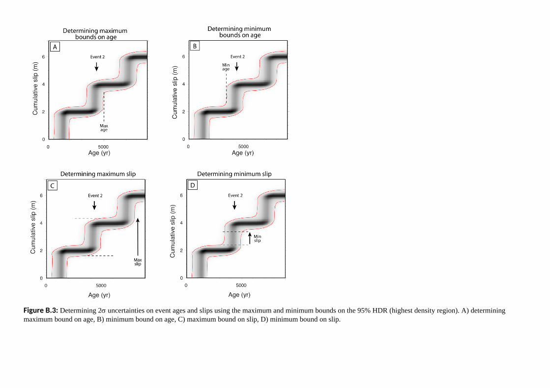
Figure B.3: Determining 2 uncertainties on event ages and slips using the maximum and minimum bounds on the 95% HDR (highest density region). A) determining maximum bound on age, B) minimum bound on age, C) maximum bound on slip, D) minimum bound on slip.

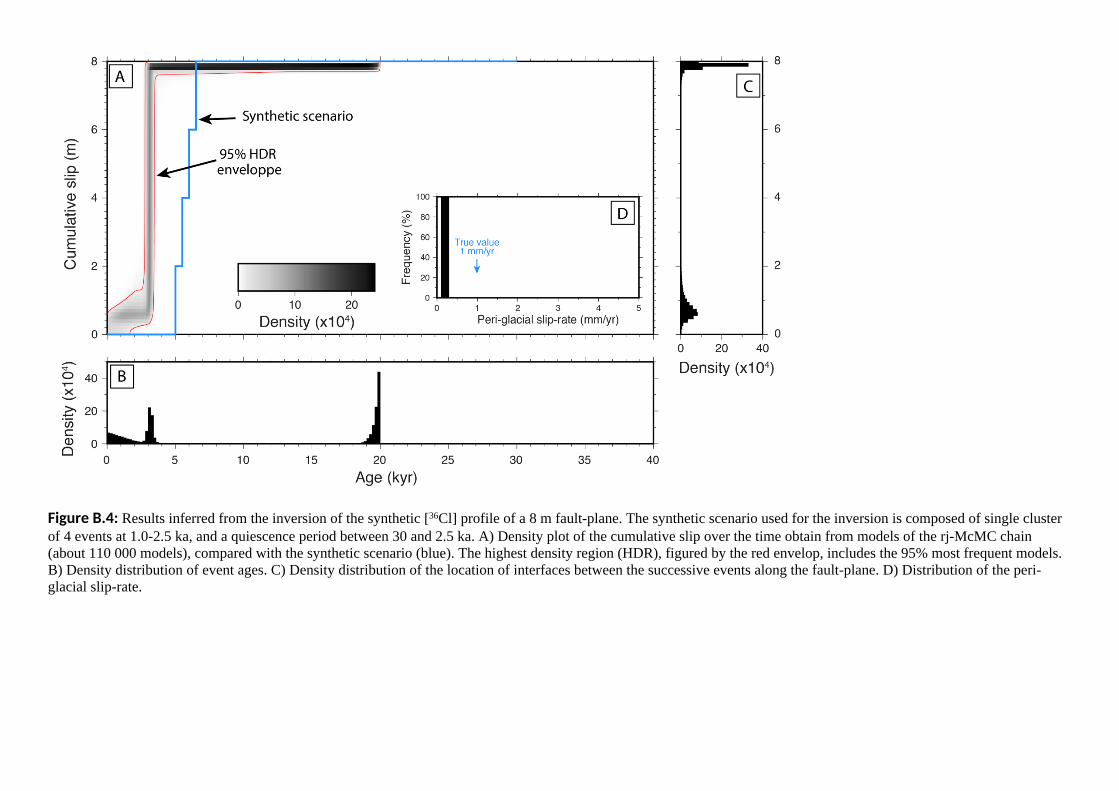
Figure B.4: Results inferred from the inversion of the synthetic [36Cl] profile of a 8 m fault-plane. The synthetic scenario used for the inversion is composed of single cluster of 4 events at 1.0-2.5 ka, and a quiescence period between 30 and 2.5 ka. A) Density plot of the cumulative slip over the time obtain from models of the rj-McMC chain (about 110 000 models), compared with the synthetic scenario (blue). The highest density region (HDR), figured by the red envelop, includes the 95% most frequent models. B) Density distribution of event ages. C) Density distribution of the location of interfaces between the successive events along the fault-plane. D) Distribution of the peri-glacial slip-rate.

Figure B.5: Results inferred from the inversion of the synthetic [36Cl] profile of a 8 m fault-plane. The synthetic scenario used for the inversion is composed of single cluster of 4 events at 1.0-2.5 ka, and a quiescence period between 30 and 2.5 ka. The synthetic [36Cl] profile (black dots) is compared with the [36Cl] profile of the best model (red line).

Figure B.6: Results inferred from the inversion of the synthetic [36Cl] profile of a 8 m fault-plane. The synthetic scenario used for the inversion is composed of single cluster of 4 events at 4.5-6.0 ka, and a quiescence period between 30 and 6.0 ka. The synthetic [36Cl] profile (black dots) is compared with the [36Cl] profile of the best model (red line).

Figure B.7: Results inferred from the inversion of the synthetic [36Cl] profile of a 8 m fault-plane, in the case of a slow-slipping fault. The synthetic scenario used for the inversion is composed of a cluster of 4 events at 5.0, 5.5, 15.0 and 15.5 ka, and a peri-glacial inheritance produced by a peri-glacial denudation of 30 m/Myr. The synthetic [36Cl] profile (black dots) is compared with the [36Cl] profile of the best model (red line, RMSw = 2.9).
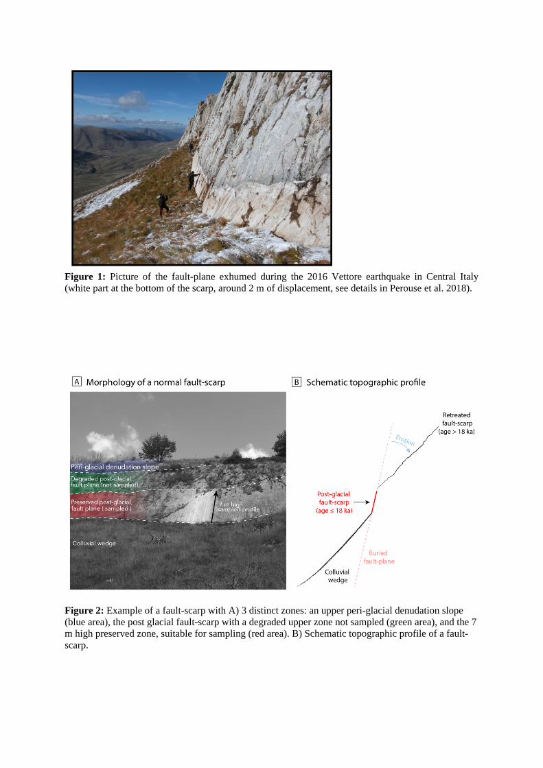
Figure 1: Picture of the fault-plane exhumed during the 2016 Vettore earthquake in Central Italy (white part at the bottom of the scarp, around 2 m of displacement, see details in Perouse et al. 2018).
Figure 2: Example of a fault-scarp with A) 3 distinct zones: an upper peri-glacial denudation slope (blue area), the post glacial fault-scarp with a degraded upper zone not sampled (green area), and the 7 m high preserved zone, suitable for sampling (red area). B) Schematic topographic profile of a fault-scarp.
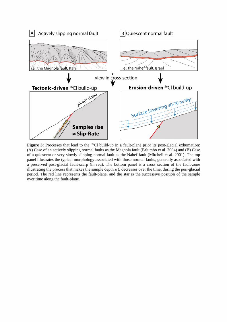
Figure 3: Processes that lead to the 36Cl build-up in a fault-plane prior its post-glacial exhumation: (A) Case of an actively slipping normal faults as the Magnola fault (Palumbo et al. 2004) and (B) Case of a quiescent or very slowly slipping normal fault as the Nahef fault (Mitchell et al. 2001). The top panel illustrates the typical morphology associated with those normal faults, generally associated with a preserved post-glacial fault-scarp (in red). The bottom panel is a cross section of the fault-zone illustrating the process that makes the sample depth z(t) decreases over the time, during the peri-glacial period. The red line represents the fault-plane, and the star is the successive position of the sample over time along the fault-plane.

Figure 4: Deconvolution of the three 36Cl uptake on a fault scarp: 1) during the long-term inheritance period (here slip-rate 1 mm/yr, left panel), 2) during the exhumation of the upper fault scarp portion, too eroded to be sampled, that we will called the post-glacial inheritance (here at 10, 12, 14 and 16 ka with 2 m of slip per event, central panel), and 3) during the exhumation of the preserved sampled fault-plane (called the post-glacial exhumation, here at 2, 4, 6 and 8 ka with a slip per event of 2 m, right panel). The dashed line represents the 36Cl accumulated during the considered period, and the black line represent the final [36Cl] profile.

Figure 5: Each model is parameterized by a variable number of event k (here 4) that exhumed several portion i of the fault-plane, each portion of the fault-plane having an age ai. The geometry of the exhumed portion of the fault-plane is described using Voronoi nuclei ci (square). The vertical position(s) of the nuclei ci determine the location of the interface(s) between each exhumed portion (dashed lines), defined as the equidistant between adjacent nuclei. The nuclei are thus not necessary in the middle of a portion. The slip si of each event i is obtained by the size of the exhumed portion. The black curve represents the slip over the time of the model.
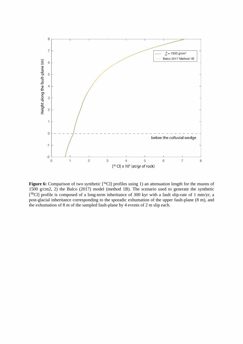
Figure 6: Comparison of two synthetic [36Cl] profiles using 1) an attenuation length for the muons of 1500 g/cm2, 2) the Balco (2017) model (method 1B). The scenario used to generate the synthetic [36Cl] profile is composed of a long-term inheritance of 300 kyr with a fault slip-rate of 1 mm/yr, a post-glacial inheritance corresponding to the sporadic exhumation of the upper fault-plane (8 m), and the exhumation of 8 m of the sampled fault-plane by 4 events of 2 m slip each.
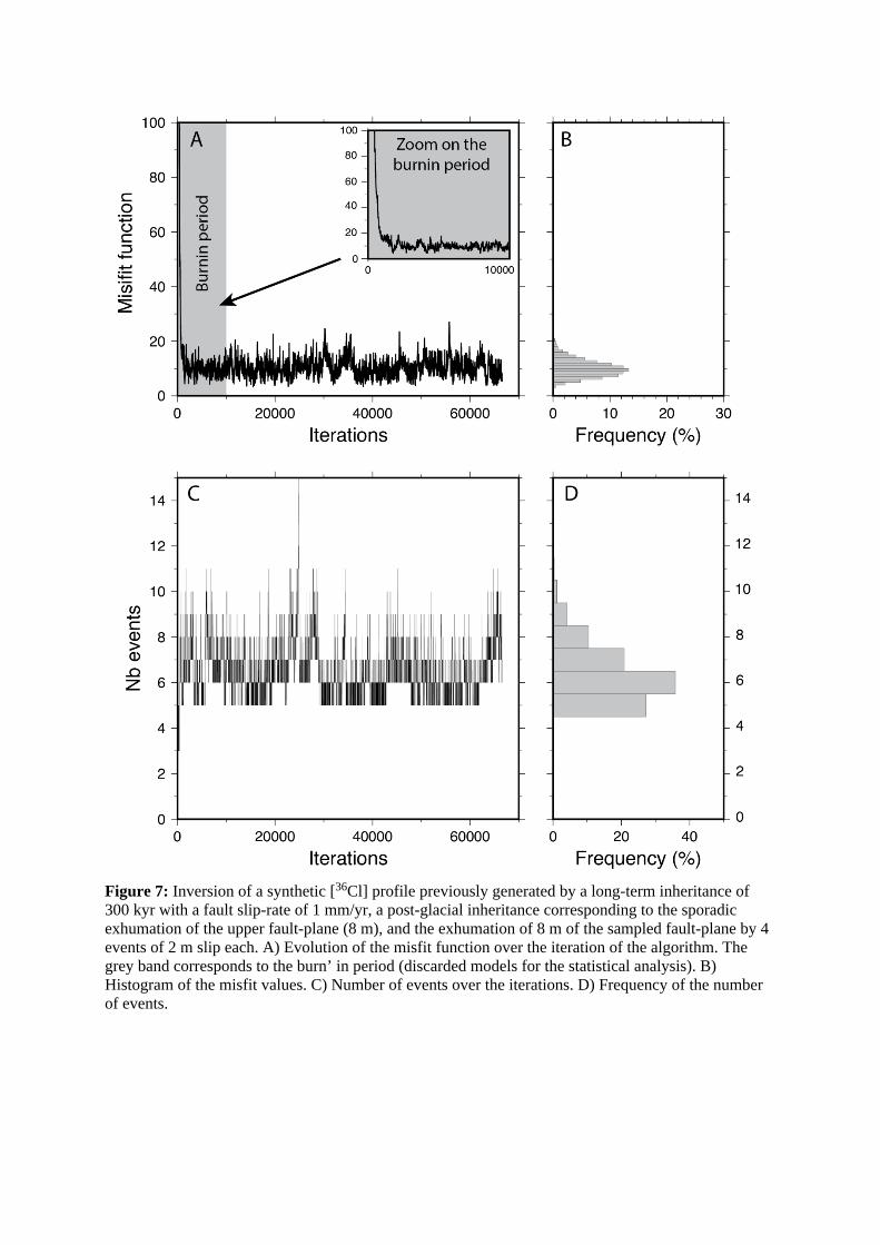
Figure 7: Inversion of a synthetic [36Cl] profile previously generated by a long-term inheritance of 300 kyr with a fault slip-rate of 1 mm/yr, a post-glacial inheritance corresponding to the sporadic exhumation of the upper fault-plane (8 m), and the exhumation of 8 m of the sampled fault-plane by 4 events of 2 m slip each. A) Evolution of the misfit function over the iteration of the algorithm. The grey band corresponds to the burn’ in period (discarded models for the statistical analysis). B) Histogram of the misfit values. C) Number of events over the iterations. D) Frequency of the number of events.

Figure 8: Results inferred from the inversion of the synthetic [36Cl] profile of a fault-plane sampled up to 8 m. A) Density plot of the cumulative slip over time obtained from models of the rj-McMC chain (about 740 000 models), compared with the true scenario (blue). The highest density region (HDR), figured by the red envelop, includes the 95% most frequent models. B) Density distribution of event ages. C) Density distribution of the interfaces location between successive events along the fault-plane. D) Distribution of the yielded peri-glacial slip-rate.

Figure 9: Comparison between modeled [36Cl] profiles from the 100 best models obtained from the inversion (red lines), and the synthetic [36Cl] profile (black dots with 2 uncertainties).
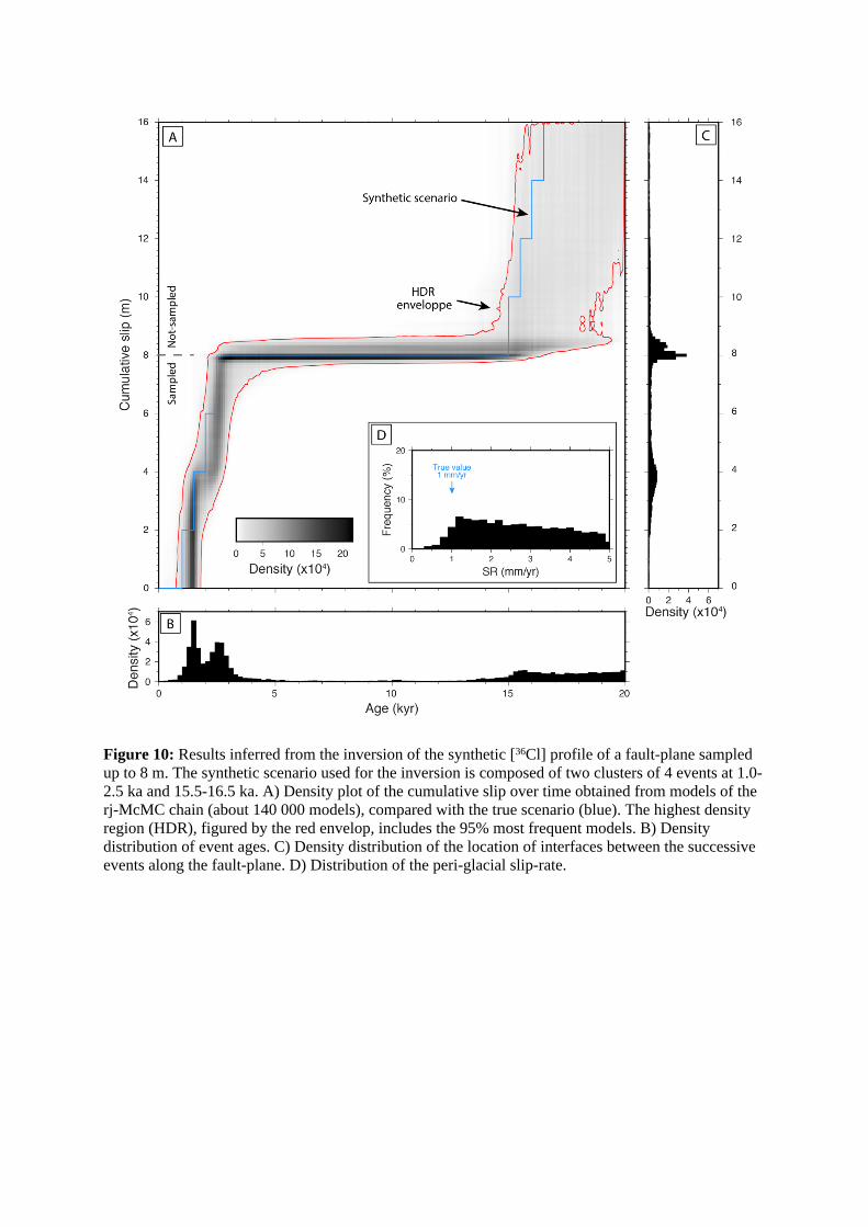
Figure 10: Results inferred from the inversion of the synthetic [36Cl] profile of a fault-plane sampled up to 8 m. The synthetic scenario used for the inversion is composed of two clusters of 4 events at 1.0-2.5 ka and 15.5-16.5 ka. A) Density plot of the cumulative slip over time obtained from models of the rj-McMC chain (about 140 000 models), compared with the true scenario (blue). The highest density region (HDR), figured by the red envelop, includes the 95% most frequent models. B) Density distribution of event ages. C) Density distribution of the location of interfaces between the successive events along the fault-plane. D) Distribution of the peri-glacial slip-rate.

Figure 11: Results inferred from the inversion of the synthetic [36Cl] profile of a fault-plane sampled up to 8 m. The synthetic scenario used for the inversion is composed of two cluster of 4 events at 1.0-2.5 ka and 15.5-16.5 ka, and a quiescence period between 30 and 16.5 ka. A) Density plot of the cumulative slip over the time obtain from models of the rj-McMC chain (about 140 000 models), compared with the synthetic scenario (blue). The highest density region (HDR), figured by the red envelop, includes the 95% most frequent models. B) Density distribution of event ages. C) Density distribution of the location of interfaces between the successive events along the fault-plane. D) Distribution of the peri-glacial slip-rate.

Figure 12: Results inferred from the inversion of the synthetic [36Cl] profile of a 8m high fault-plane, sampled up to the top. The synthetic scenario used for the inversion is composed of a cluster of 4 events between 5.0 and 6.5 ka, and a quiescence period between 30 ka and 6.5 ka. A) Density plot of the cumulative slip over time obtained from models of the rj-McMC chain (about 190 000 models), compared with the true scenario (blue). The highest density region (HDR), figured by the red envelop, includes the 95% most frequent models. B) Density distribution of event ages in black, and of the starting of the quiescence period in grey. C) Density distribution of the location of interfaces between the successive events along the fault-plane. D) Distribution of the peri-glacial slip-rate, prior the quiescence period.
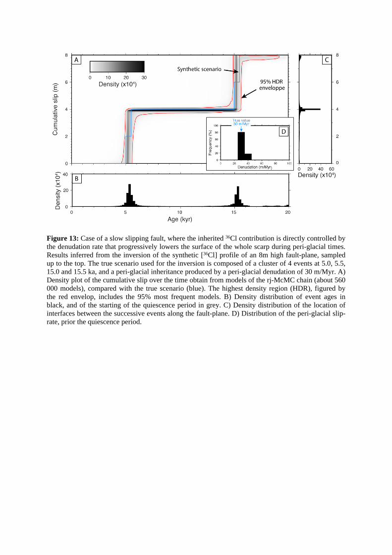
Figure 13: Case of a slow slipping fault, where the inherited 36Cl contribution is directly controlled by the denudation rate that progressively lowers the surface of the whole scarp during peri-glacial times. Results inferred from the inversion of the synthetic [36Cl] profile of an 8m high fault-plane, sampled up to the top. The true scenario used for the inversion is composed of a cluster of 4 events at 5.0, 5.5, 15.0 and 15.5 ka, and a peri-glacial inheritance produced by a peri-glacial denudation of 30 m/Myr. A) Density plot of the cumulative slip over the time obtain from models of the rj-McMC chain (about 560 000 models), compared with the true scenario (blue). The highest density region (HDR), figured by the red envelop, includes the 95% most frequent models. B) Density distribution of event ages in black, and of the starting of the quiescence period in grey. C) Density distribution of the location of interfaces between the successive events along the fault-plane. D) Distribution of the peri-glacial slip-rate, prior the quiescence period.

Figure 14: 36Cl profiles as function of depth below the surface of the colluvial wedge. Dark line is scenario produced with a fault plane initially exposed at depth during 300 kyr with a fault slip-rate of 0.5 mm/yr and then exhumed by sporadic events during 10 kyr (8 m of total displacement). The dashed line is the 36Cl profile derived from the same post-glacial exhumation but with no long-term inheritance and only considering a fixed amount of pre-exposure prior the post-glacial exhumation as done in Schlagenhauf et al. (2010) (here pre-exposure is 7 kyr). The right panel indicates the difference between the two curves.


