Section 7.2: Direction Fields and Euler’s Methods
Practice HW from Stewart Textbook (not to hand in)
p. 511 # 1-13, 19-23 odd
For a given differential equation, we want to look
at ways to find its solution. In this chapter, we will
examine 3 techniques for determining the
behavior for the solution. These techniques will
involve looking at the solutions graphically,
numerically, and analytically.
Examining Solutions Graphically – Direction Fields
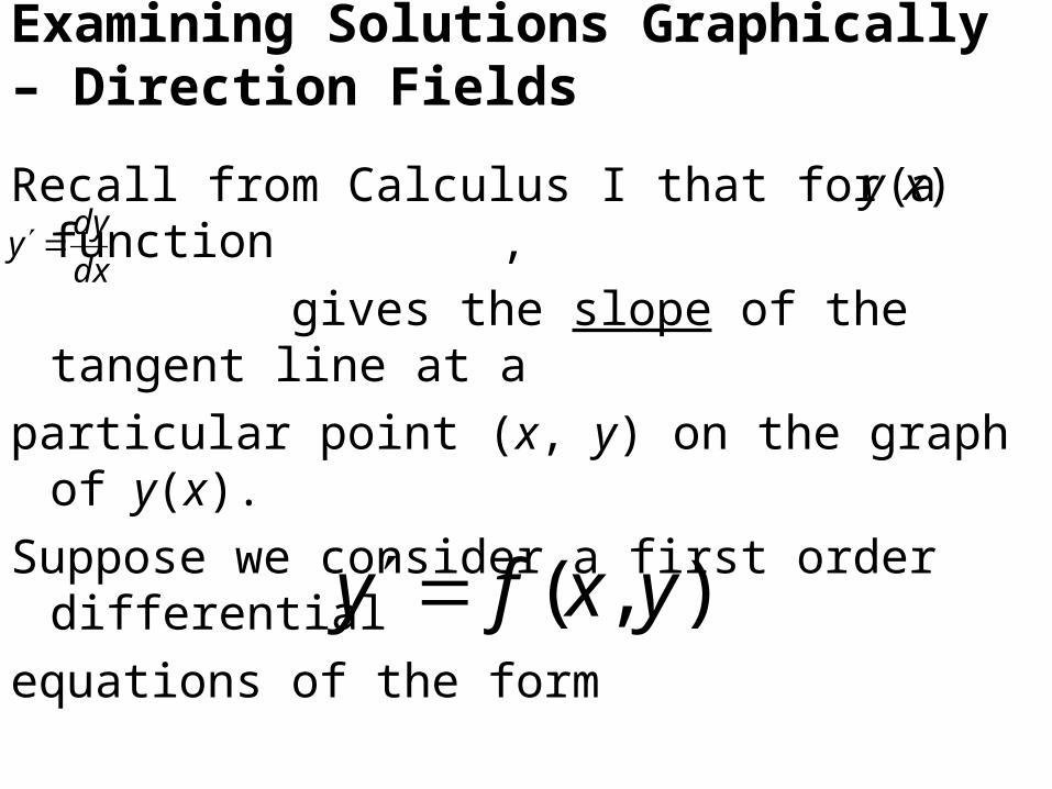
Recall from Calculus I that for a function ,
gives the slope of the tangent line at a
particular point (x, y) on the graph of y(x).
Suppose we consider a first order differential
equations of the form
)(xy
dx
dyy
),( yxfy

For a solution y of this differential equation,
evaluated at the point represents the
slope of the tangent line to the graph of y(x) at
this point.
y),( 11 yx
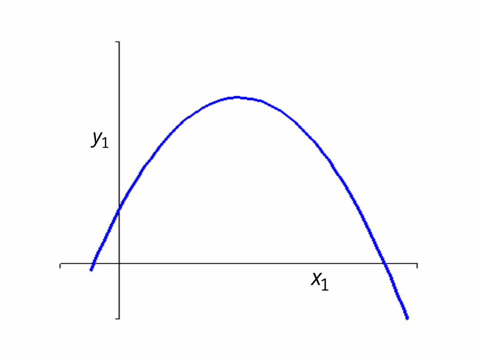
1x
1y
Even though we do not know the formula for the
solution y(x), having the differential equation
gives a convenient way for calculating
the tangent line slopes at various points. If we
obtain these slopes for many points, we can get a
good general idea of how the solution is
behaving.
),( yxfy
Direction Fields (sometimes called slope fields)
involves a method for determining the behavior of
various solutions on the x-y plane by calculating
the tangent line slopes at various points.
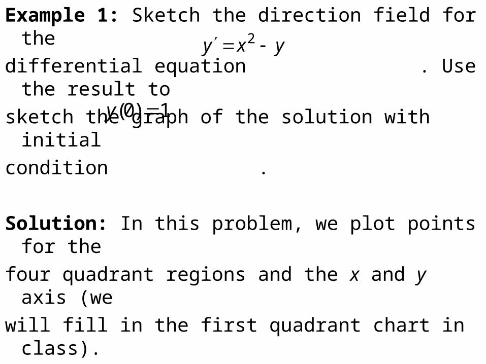
Example 1: Sketch the direction field for the
differential equation . Use the result to
sketch the graph of the solution with initial
condition .
Solution: In this problem, we plot points for the
four quadrant regions and the x and y axis (we
will fill in the first quadrant chart in class).
yxy 2
1)0( y
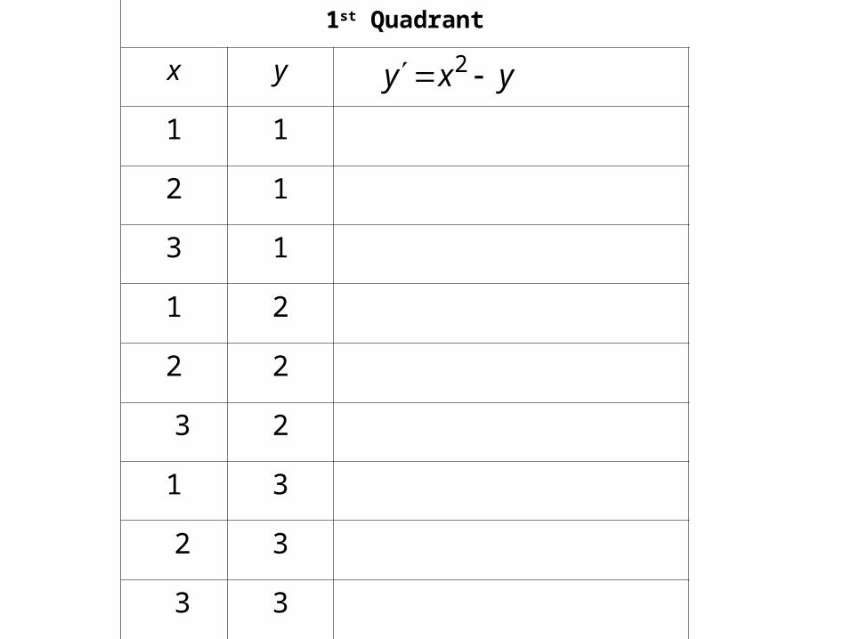
yxy 2
1st Quadrant
x y
1 1
2 1
3 1
1 2
2 2
3 2
1 3
2 3
3 3

We can sketch the slopes on the following graph
(will do in class):
x
y

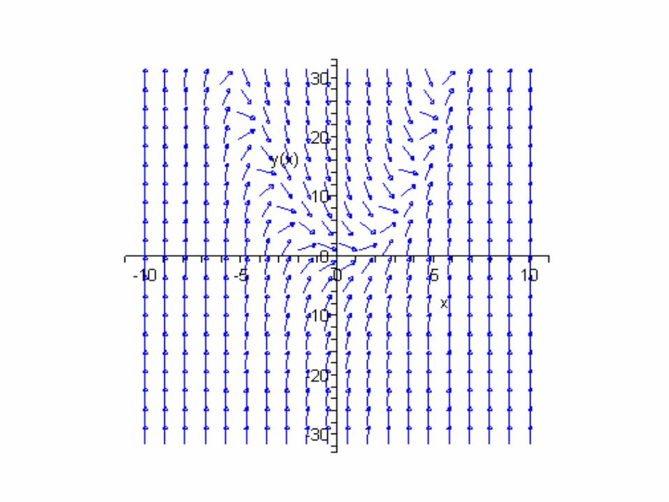
Obviously, as can be seen by the last example,
sketching direction fields by hand can be a very
tedious task. However, Maple can sketch a
direction field quickly. For the differential equation
given in Example 1, the following
commands in Maple can be used to sketch the
direction field:
yxy 2
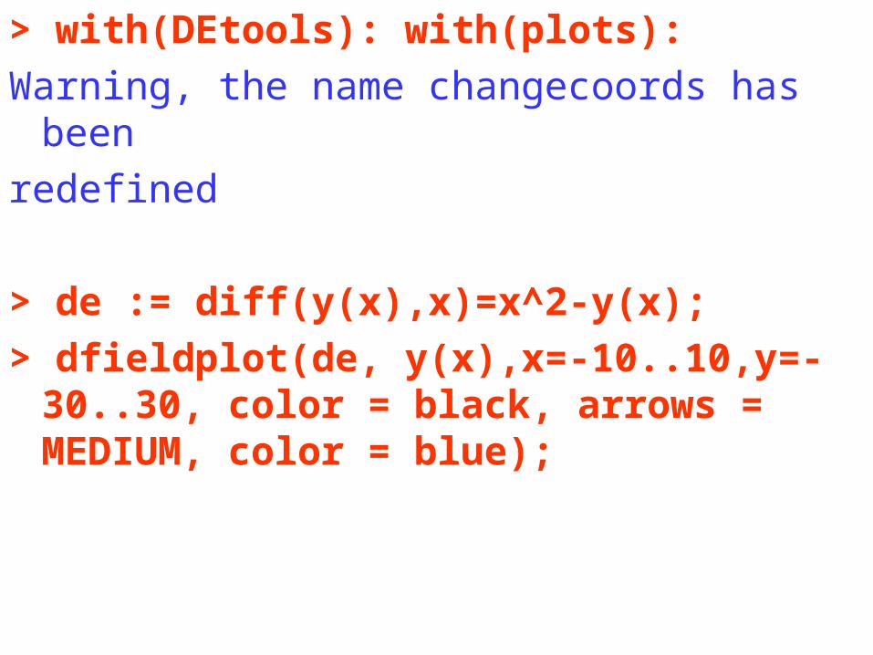
> with(DEtools): with(plots):
Warning, the name changecoords has been
redefined
> de := diff(y(x),x)=x^2-y(x);
> dfieldplot(de, y(x),x=-10..10,y=-30..30, color = black, arrows = MEDIUM, color = blue);
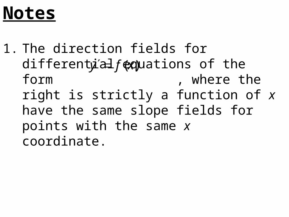
Notes
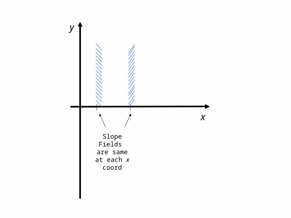
1. The direction fields for differential equations of the form , where the right is strictly a function of x have the same slope fields for points with the same x coordinate.
)(xfy
x
y
Slope Fields are same at
each x coord
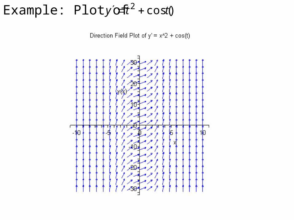
Example: Plot of )cos(2 tty
2.The direction fields for differential equations of
the form , where the right is strictly a
function of y have the same slope fields for
points with the same y coordinate. A differential equation is strictly a function of the dependent variable y is known as an autonomous equation.
)(yfy
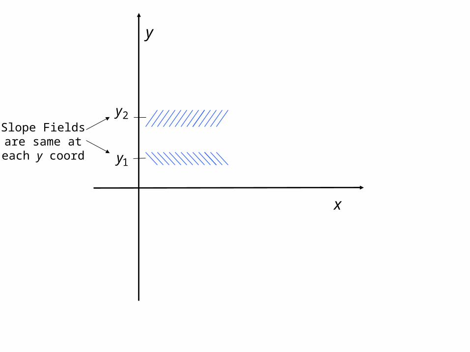
x
y
Slope Fields are same at each y coord
1y
2y
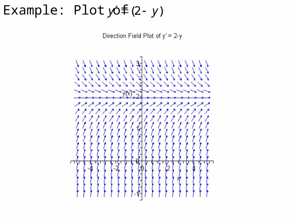
Example: Plot of )2( yy
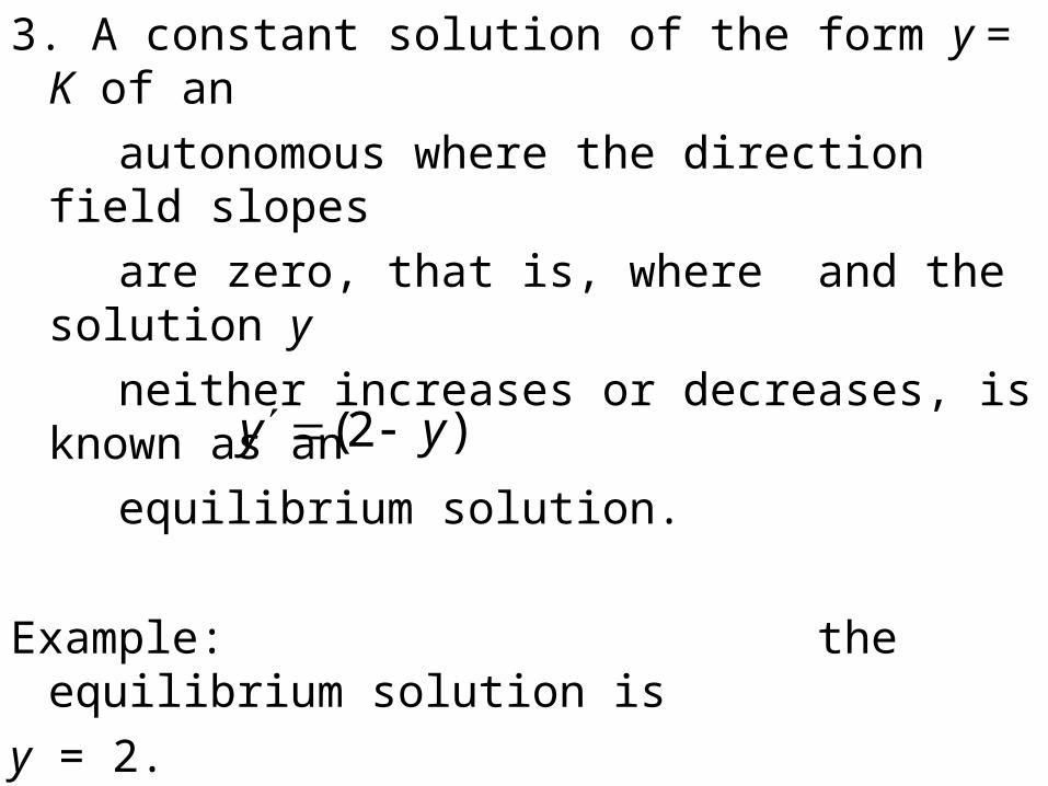
3. A constant solution of the form y = K of an
autonomous where the direction field slopes
are zero, that is, where and the solution y
neither increases or decreases, is known as an
equilibrium solution.
Example: the equilibrium solution is
y = 2.
)2( yy
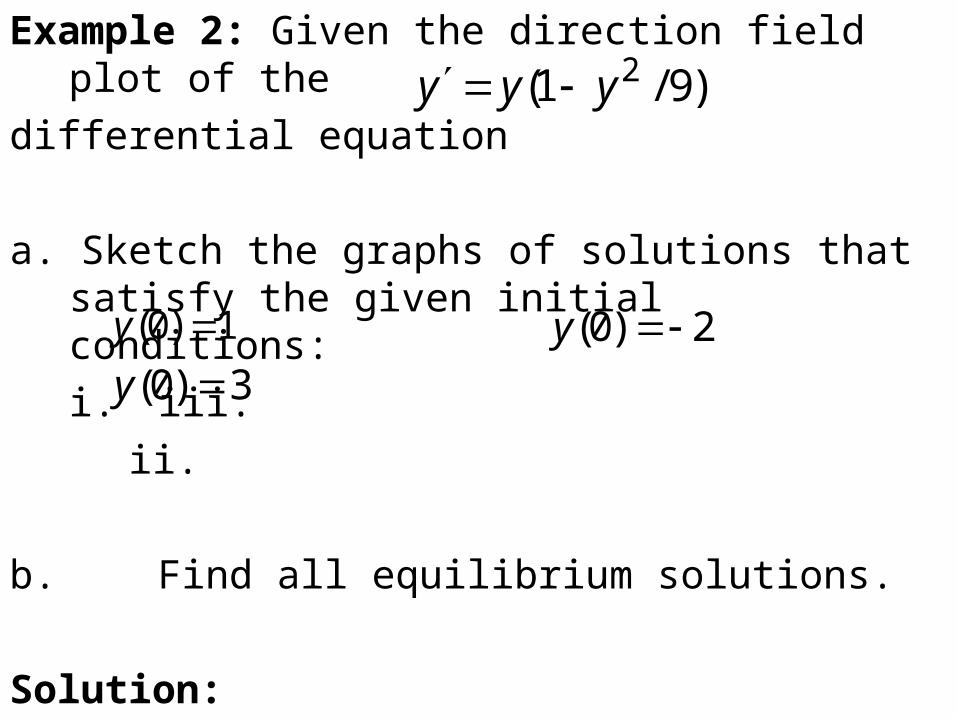
Example 2: Given the direction field plot of the
differential equation
a. Sketch the graphs of solutions that satisfy the given initial conditions:
i. iii.
ii.
b. Find all equilibrium solutions.
Solution:
)9/1( 2yyy
1)0( y
3)0( y
2)0( y

Finding Solutions Numerically – Euler’s Method
A common way to examine the solution of a
differential equations is to approximate it
numerically. One of the more simpler methods for
doing this involves Euler’s method.
Consider the initial value problem
.
over the interval . Suppose we want
to find an approximation to the solution y(x) given
by the following graph:
00 )( ),,( yxyyxFy
bxax 0
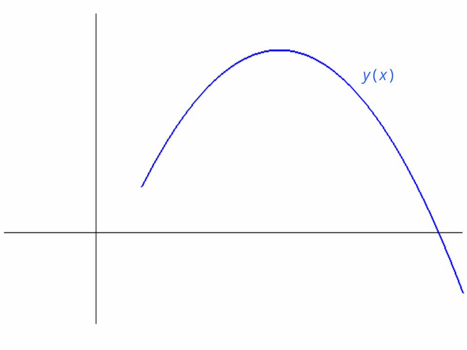
y(x)
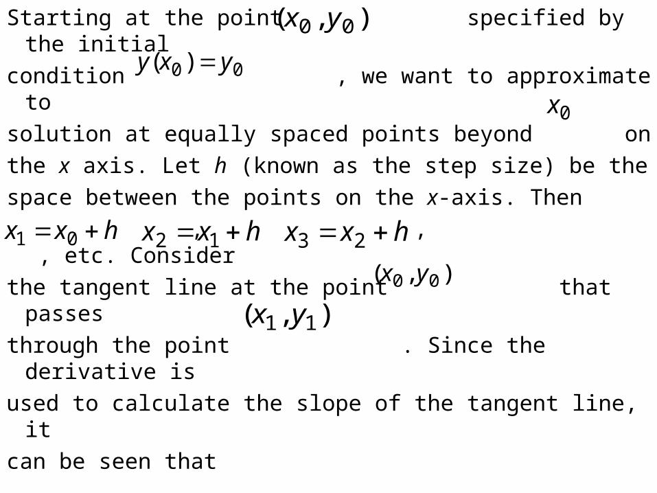
Starting at the point specified by the initial
condition , we want to approximate to
solution at equally spaced points beyond on
the x axis. Let h (known as the step size) be the
space between the points on the x-axis. Then
, , , etc. Consider
the tangent line at the point that passes
through the point . Since the derivative is
used to calculate the slope of the tangent line, it
can be seen that
),( 00 yx
00 )( yxy
0x
hxx 01 hxx 12 hxx 23
),( 00 yx
),( 11 yx
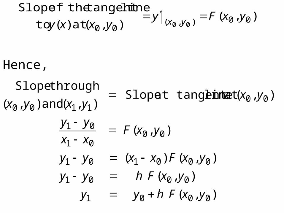
Hence,
),(),(at )( to
line tangent theof Slope00),(
00 00yxFy
yxxy yx
),(
),(
),( )(
),(
),(at line at tangent Slope ),( and ),(
throughSlope
0001
0001
000101
0001
01
001100
yxFhyy
yxFhyy
yxFxxyy
yxFxx
yy
yxyxyx

Now, consider the line through the points
and .
),( 11 yx
),( 22 yx
),(
),(
),(),(at line at tangent Slope ),( and ),(
throughSlope
1112
1112
12
11112211
yxFhyy
yxFxx
yy
yxFyxyxyx
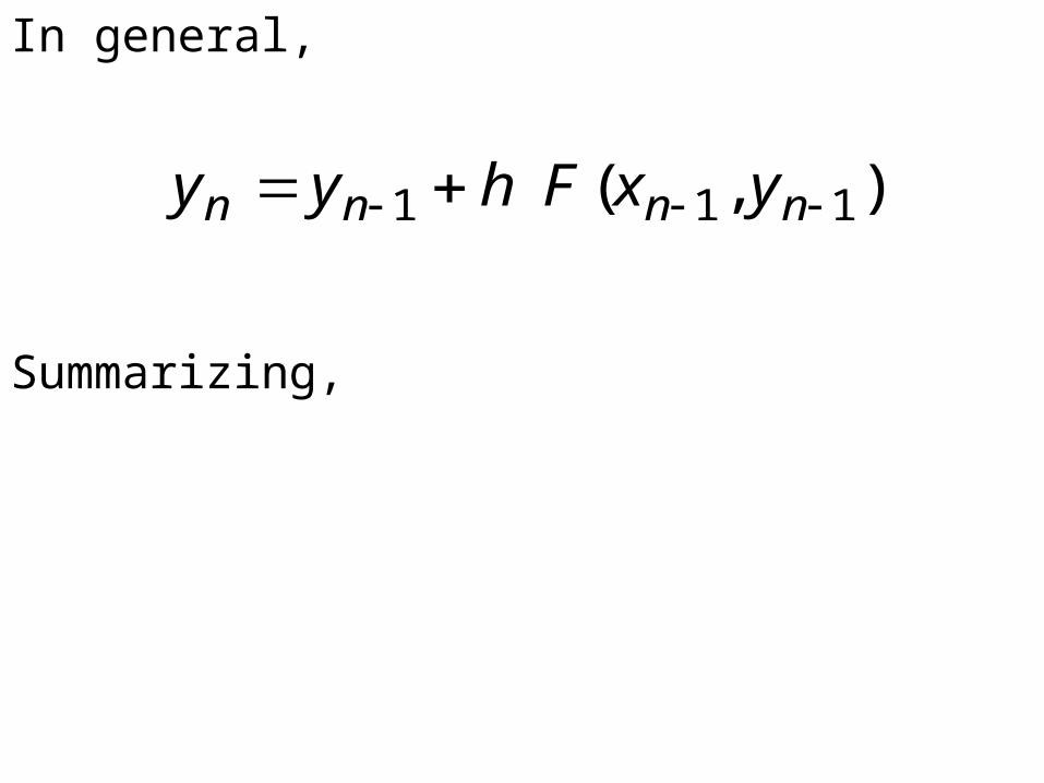
In general,
Summarizing,
),( 111 nnnn yxFhyy
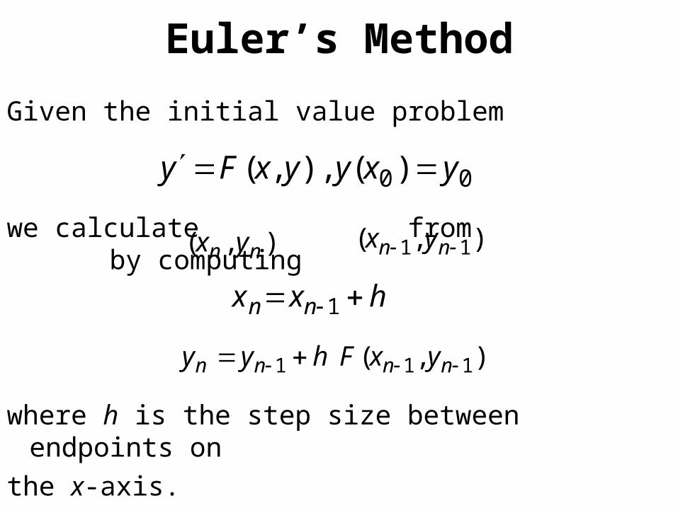
Euler’s Method
Given the initial value problem
we calculate from by computing
where h is the step size between endpoints on
the x-axis.
00 )( ),,( yxyyxFy
),( nn yx ),( 11 nn yx
hxx nn 1
),( 111 nnnn yxFhyy
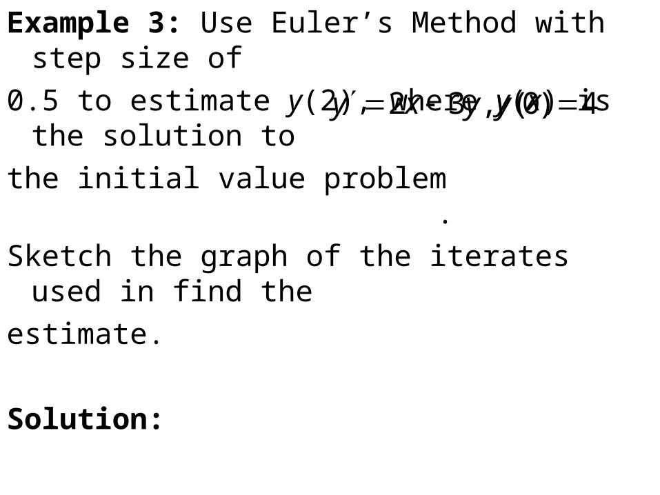
Example 3: Use Euler’s Method with step size of
0.5 to estimate y(2), where y(x) is the solution to
the initial value problem .
Sketch the graph of the iterates used in find the
estimate.
Solution:
4)0( ,32 yyxy


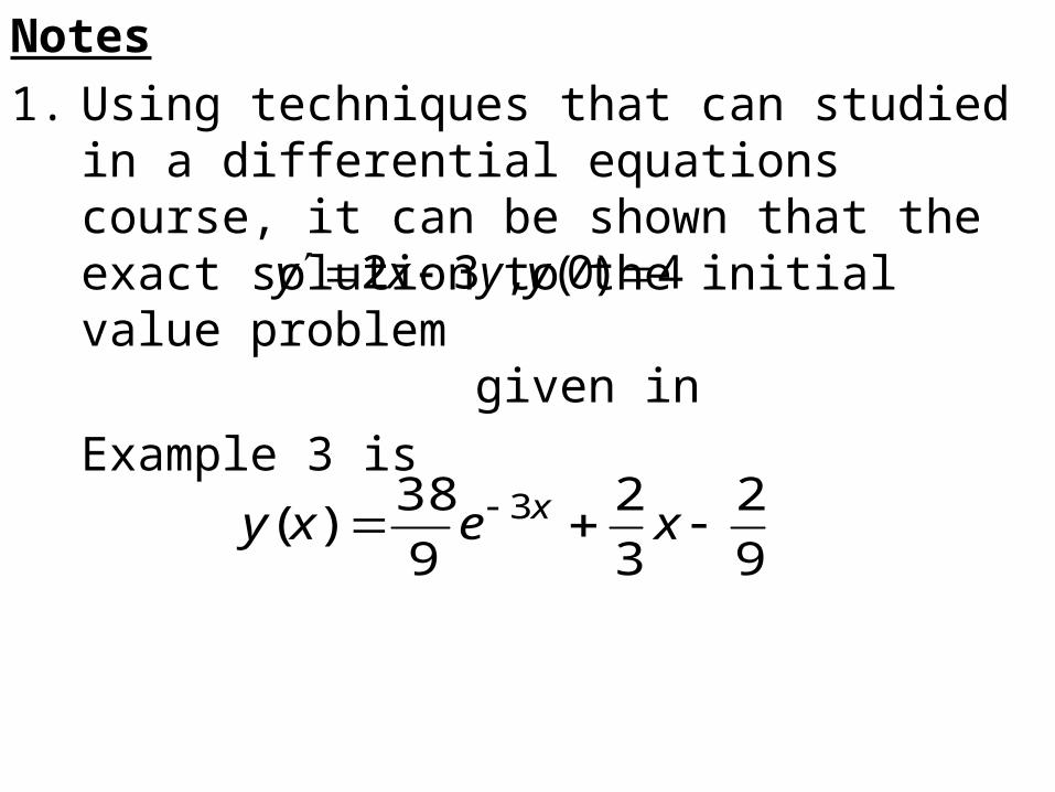
Notes
1. Using techniques that can studied in a differential equations course, it can be shown that the exact solution to the initial value problem given in
Example 3 is
9
2
3
2
9
38)( 3 xexy x
4)0( ,32 yyxy
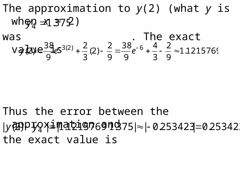
The approximation to y(2) (what y is when x = 2)
was . The exact value is
Thus the error between the approximation and
the exact value is
375.14 y
.1215769.19
2
3
4
9
38
9
2)2(
3
2
9
38)2( 6)2(3 eey
253423.0 |253423.0| |375.11215769.1| |)2(| 4 yy
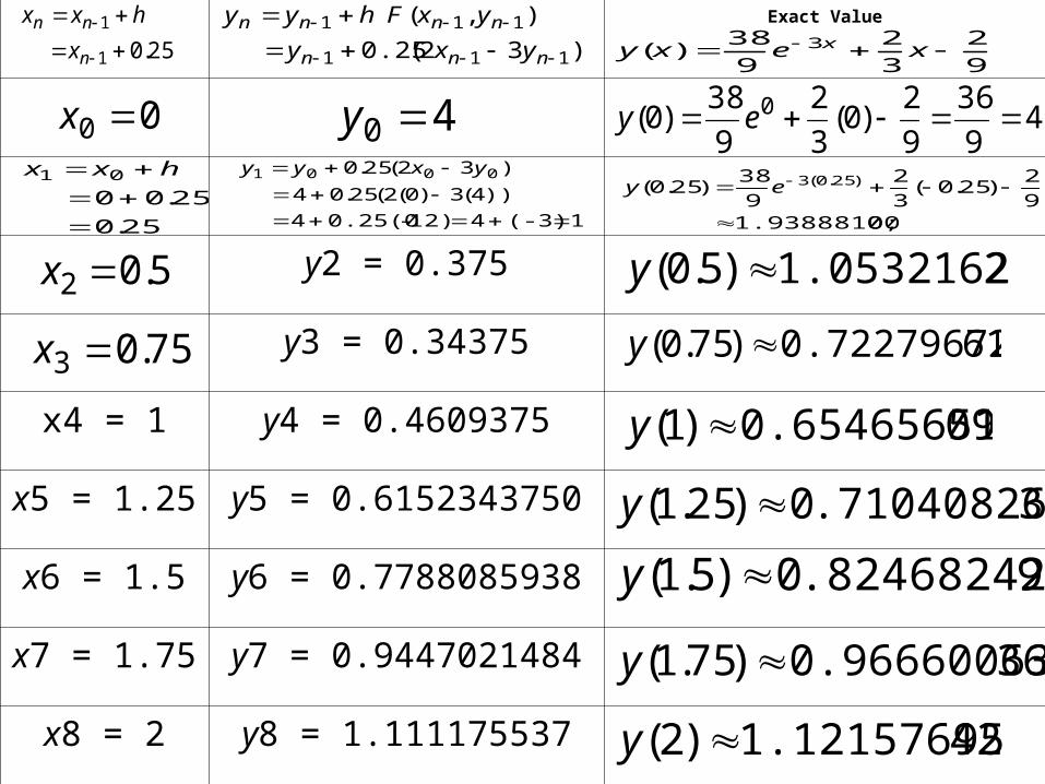
2.By decreasing the step size h, the accuracy of the approximation in most cases will be better, with a tradeoff in more work needed to achieve the approximations. For example, the chart below shows the approximations generated when the step size for Example 3 is cut in half to h = 0.25.
Exact Value
y2 = 0.375
y3 = 0.34375
x4 = 1 y4 = 0.4609375
x5 = 1.25 y5 = 0.6152343750
x6 = 1.5 y6 = 0.7788085938
x7 = 1.75 y7 = 0.9447021484
x8 = 2 y8 = 1.111175537
25.0 1
1
n
nn
x
hxx
)32(0.25
),(
111
111
nnn
nnnn
yxy
yxFhyy
9
2
3
2
9
38)( 3 xexy x
00 x
25.0
25.00 01
hxx
5.02 x
40 y
1(-3)412)-0.25(04
))4(3)0(2(25.04
)32(25.0 0001
yxyy
75.03 x
49
36
9
2)0(
3
2
9
38)0( 0 ey
0;1.93888100 9
2)25.0(
3
2
9
38)25.0( )25.0(3
ey
21.05321623)5.0( y
610.72279672)75.0( y
090.65465651)1( y
3.7104082600)25.1( y
9.8246824290)5.1( y
360.96660063)75.1( y
421.12157695)2( y
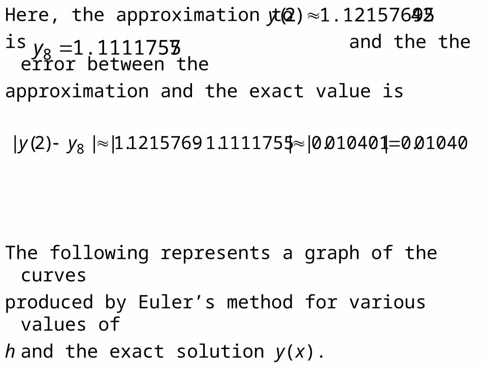
Here, the approximation to
is and the the error between the
approximation and the exact value is
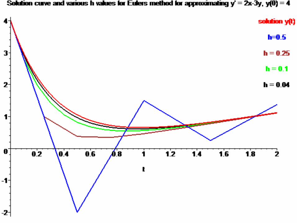
The following represents a graph of the curves
produced by Euler’s method for various values of
h and the exact solution y(x).
421.12157695)2( y
71.111175538 y
010401.0 |010401.0| |1111755.11215769.1| |)2(| 8 yy
3.There are other numerical methods that can achieve better accuracy with less work than Euler’s method. However, the underlying approach used in many of these methods stem from Euler’s approach.


