Download - Search and Intersection

Search and Intersection
O’Rourke, Chapter 7
Outline
• Trapezoidal Decomposition
• Extreme Points (2D)
• Extreme Points (3D)

Goal:
Given a set of line segments partition space into
trapezoids with horizontal tops/bottoms so that each
trapezoid has unique left/right
neighbors.*
Trapezoidal Decomposition
𝑎1
𝑏1
𝑎2
𝑏2
𝑐1
𝑐2
𝑑2
𝑑1
*Assume no line segment is vertical.

Goal:
Given a partition of 2D space into polygons,
(efficiently) compute a (compact) data-structure that
enables fast point-in-polygon queries.
Example (Nearest-Neighbor):
Given the Voronoi diagram of
a set of points, we would like
to quickly determine to which
Voronoi cell a point belongs.
Trapezoidal Decomposition

Approach:
Construct the partition iteratively, adding new line-
segments into existing partition:
Add end-point, performing top/bottom split of
containing trapezoid.
Trapezoidal Decomposition
𝐴
𝐴
𝑝

Approach:
Construct the partition iteratively, adding new line-
segments into existing partition:
Add end-point, performing top/bottom split of
containing trapezoid.
Trapezoidal Decomposition
𝐵
𝐵 𝐶
𝑌(𝑝)
𝐶𝑝

Approach:
Construct the partition iteratively, adding new line-
segments into existing partition:
Add end-point.
Add line segment, splitting the trapezoid into 2, 3, or 4
sub-trapezoids.
Trapezoidal Decomposition
𝐴
𝐴
𝑙

Approach:
Construct the partition iteratively, adding new line-
segments into existing partition:
Add end-point.
Add line segment, splitting the trapezoid into 2, 3, or 4
sub-trapezoids.
Trapezoidal Decomposition
𝐵 𝐶
𝑋(𝑙)
𝐵 𝐶
𝑙

Approach:
Construct the partition iteratively, adding new line-
segments into existing partition:
Add end-point.
Add line segment, splitting the trapezoid into 2, 3, or 4
sub-trapezoids.
Trapezoidal Decomposition
𝐴
𝐴 𝑙
𝑝

Approach:
Construct the partition iteratively, adding new line-
segments into existing partition:
Add end-point.
Add line segment, splitting the trapezoid into 2, 3, or 4
sub-trapezoids.
Trapezoidal Decomposition
𝐵𝐵 𝐶
𝑙𝑌(𝑝)
𝑝
𝐶

Approach:
Construct the partition iteratively, adding new line-
segments into existing partition:
Add end-point.
Add line segment, splitting the trapezoid into 2, 3, or 4
sub-trapezoids.
Trapezoidal Decomposition
𝐷𝐸
𝑋(𝑙) 𝐶
𝑙𝑌(𝑝)
𝑝
𝐶𝐷 𝐸

Approach:
Construct the partition iteratively, adding new line-
segments into existing partition:
Add end-point.
Add line segment, splitting the trapezoid into 2, 3, or 4
sub-trapezoids.
Trapezoidal Decomposition
𝐴
𝐴𝑙
𝑝
𝑞

Approach:
Construct the partition iteratively, adding new line-
segments into existing partition:
Add end-point.
Add line segment, splitting the trapezoid into 2, 3, or 4
sub-trapezoids.
Trapezoidal Decomposition
𝐵
𝐵 𝐶𝑙
𝑌(𝑝)
𝑝
𝐶
𝑞

Approach:
Construct the partition iteratively, adding new line-
segments into existing partition:
Add end-point.
Add line segment, splitting the trapezoid into 2, 3, or 4
sub-trapezoids.
Trapezoidal Decomposition
𝐷
𝑌(𝑞) 𝐶𝑙
𝑌(𝑝)
𝑝
𝐷 𝐸
𝐸𝑞
𝐶

Approach:
Construct the partition iteratively, adding new line-
segments into existing partition:
Add end-point.
Add line segment, splitting the trapezoid into 2, 3, or 4
sub-trapezoids.
Trapezoidal Decomposition
𝐺𝑌(𝑞) 𝐶
𝑙
𝑌(𝑝)
𝑝
𝐸𝐷 𝑋(𝑙)
𝐹𝑞
𝐹 𝐺
𝐷

Approach:
Construct the partition iteratively, adding new line-
segments into existing partition:
Add end-point.
Add line segment.
Merge vertically adjacent trapezoids
if they are bounded by the same
edges (in the same order).
Trapezoidal Decomposition
𝐵
𝐴
𝐴
𝐵
∗ ∗

Approach:
Construct the partition iteratively, adding new line-
segments into existing partition:
Add end-point.
Add line segment.
Merge vertically adjacent trapezoids
if they are bounded by the same
edges (in the same order).
Trapezoidal Decomposition
∗ ∗𝐶
𝐶
Approach:
Construct the partition iteratively, adding new line-
segments into existing partition:
Add end-point.
Add line segment.
Merge vertically adjacent trapezoids
if they are bounded by the same
edges (in the same order).
Trapezoidal Decomposition
∗ ∗
𝐶
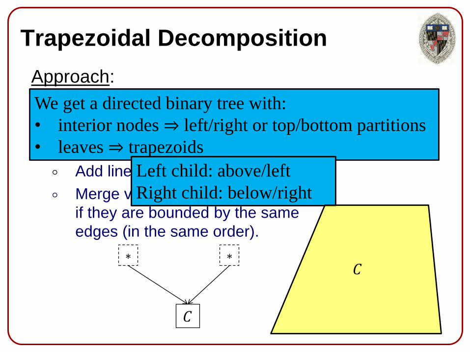
We get a directed binary tree with:
• interior nodes ⇒ left/right or top/bottom partitions
• leaves ⇒ trapezoids
Left child: above/left
Right child: below/right
𝐶
Add end-point
Add line segment
Merge adjacent trapezoids
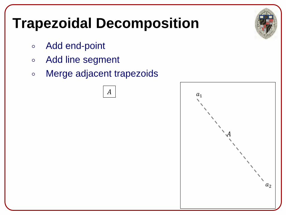
Trapezoidal Decomposition
𝐴
𝐴 𝑎1
𝑎2

Add end-point
Add line segment
Merge adjacent trapezoids
Trapezoidal Decomposition
𝐵
𝐶
𝑎1
𝑎2
𝑌(𝑎1)
𝐵 𝐶
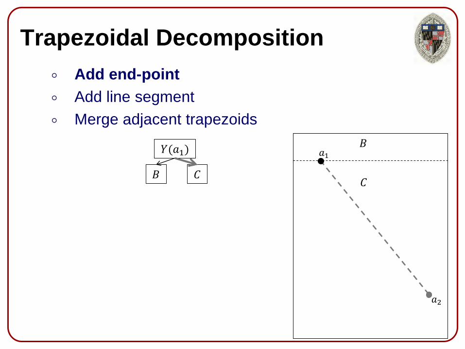
Add end-point
Add line segment
Merge adjacent trapezoids
Trapezoidal Decomposition
𝐵
𝐶
𝑎1
𝑎2
𝑌(𝑎1)
𝐵 𝐶

Add end-point
Add line segment
Merge adjacent trapezoids
Trapezoidal Decomposition
𝐵
𝐷
𝐸
𝑎1
𝑎2
𝑌(𝑎1)
𝐵 𝑌 𝑎2
𝐷 𝐸

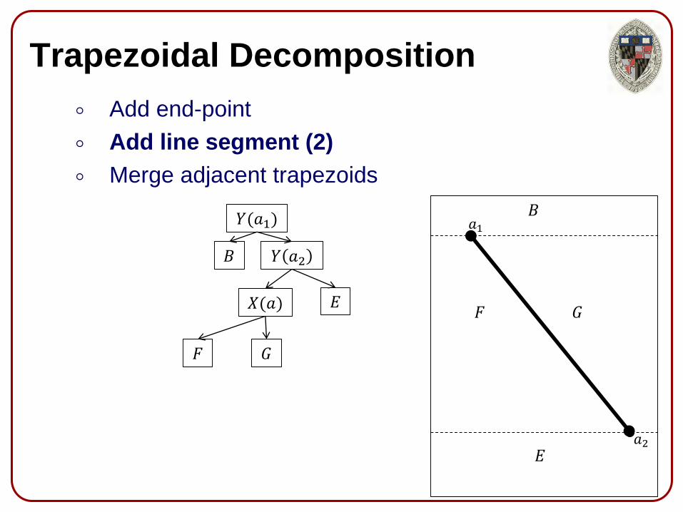
Add end-point
Add line segment (2)
Merge adjacent trapezoids
Trapezoidal Decomposition
𝐵
𝐷
𝐸
𝑎1
𝑎2
𝑌(𝑎1)
𝐵 𝑌 𝑎2
𝐷 𝐸
Add end-point
Add line segment (2)
Merge adjacent trapezoids
Trapezoidal Decomposition
𝐵
𝐸
𝐺𝐹
𝑎1
𝑎2
𝑌(𝑎1)
𝐵 𝑌 𝑎2
𝑋(𝑎) 𝐸
𝐹 𝐺

Add end-point
Add line segment
Merge adjacent trapezoids
Trapezoidal Decomposition
𝐵
𝐸
𝐺𝐹
𝑎1
𝑎2
𝑌(𝑎1)
𝐵 𝑌 𝑎2
𝑋(𝑎) 𝐸
𝐹 𝐺
𝑏1
𝑏2

Add end-point
Add line segment
Merge adjacent trapezoids
Trapezoidal Decomposition
𝐵
𝐸
𝐼𝐹
𝐻
𝑎1
𝑏1
𝑎2
𝑌(𝑎1)
𝐵 𝑌 𝑎2
𝑋(𝑎) 𝐸
𝐹 𝑌(𝑏1)
𝐻 𝐼

Add end-point
Add line segment
Merge adjacent trapezoids
Trapezoidal Decomposition
𝐵
𝐸
𝐼𝐹
𝐻
𝑎1
𝑏1
𝑎2
𝑏2
𝑌(𝑎1)
𝐵 𝑌 𝑎2
𝑋(𝑎) 𝐸
𝐹 𝑌(𝑏1)
𝐻 𝐼

Add end-point
Add line segment
Merge adjacent trapezoids
Trapezoidal Decomposition
𝐵
𝐽
𝐼𝐹
𝐻
𝐾
𝑎1
𝑏1
𝑎2
𝑏2
𝑌(𝑎1)
𝐵 𝑌 𝑎2
𝑋(𝑎) 𝑌 𝑏2
𝐹 𝑌(𝑏1)
𝐻 𝐼
𝐽 𝐾

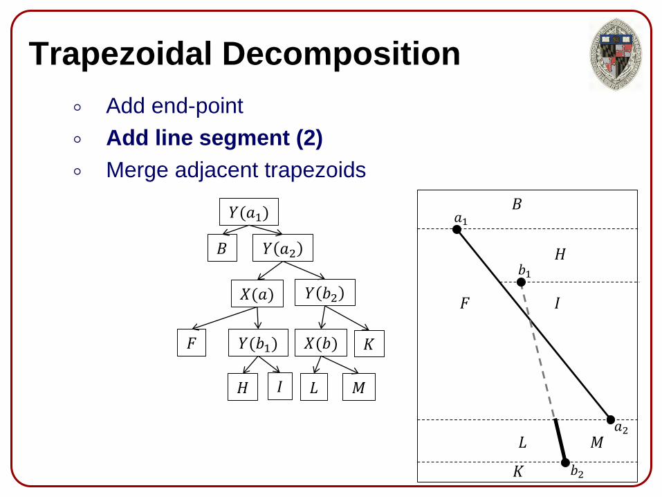
Add end-point
Add line segment (2)
Merge adjacent trapezoids
Trapezoidal Decomposition
𝐵
𝐽
𝐼𝐹
𝐻
𝐾
𝑎1
𝑏1
𝑎2
𝑏2
𝑌(𝑎1)
𝐵 𝑌 𝑎2
𝑋(𝑎) 𝑌 𝑏2
𝐹 𝑌(𝑏1)
𝐻 𝐼
𝐽 𝐾
Add end-point
Add line segment (2)
Merge adjacent trapezoids
Trapezoidal Decomposition
𝐵
𝐿
𝐼𝐹
𝐻
𝐾
𝑀
𝑎1
𝑏1
𝑎2
𝑏2
𝑌(𝑎1)
𝐵 𝑌 𝑎2
𝑋(𝑎) 𝑌 𝑏2
𝐹 𝑌(𝑏1)
𝐻 𝐼
𝑋(𝑏) 𝐾
𝑀𝐿

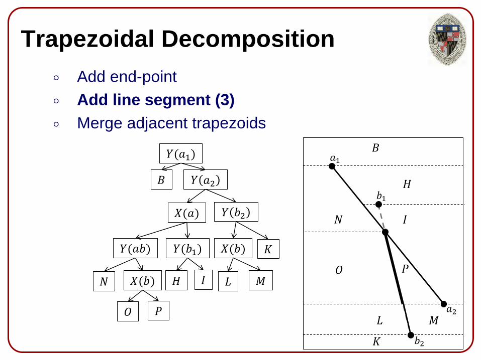
Add end-point
Add line segment (3)
Merge adjacent trapezoids
Trapezoidal Decomposition
𝐵
𝐿
𝐼𝐹
𝐻
𝐾
𝑀
𝑎1
𝑏1
𝑎2
𝑏2
𝑌(𝑎1)
𝐵 𝑌 𝑎2
𝑋(𝑎) 𝑌 𝑏2
𝐹 𝑌(𝑏1)
𝐻 𝐼
𝑋(𝑏) 𝐾
𝑀𝐿
Add end-point
Add line segment (3)
Merge adjacent trapezoids
Trapezoidal Decomposition
𝐵
𝐿
𝐼𝑁
𝐻
𝐾
𝑀
𝑂 𝑃
𝑎1
𝑏1
𝑎2
𝑏2
𝑌(𝑎1)
𝐵 𝑌 𝑎2
𝑋(𝑎) 𝑌 𝑏2
𝑌(𝑎𝑏) 𝑌(𝑏1)
𝐻 𝐼
𝑋(𝑏) 𝐾
𝑀𝑁 𝑋(𝑏)
𝑂 𝑃
𝐿

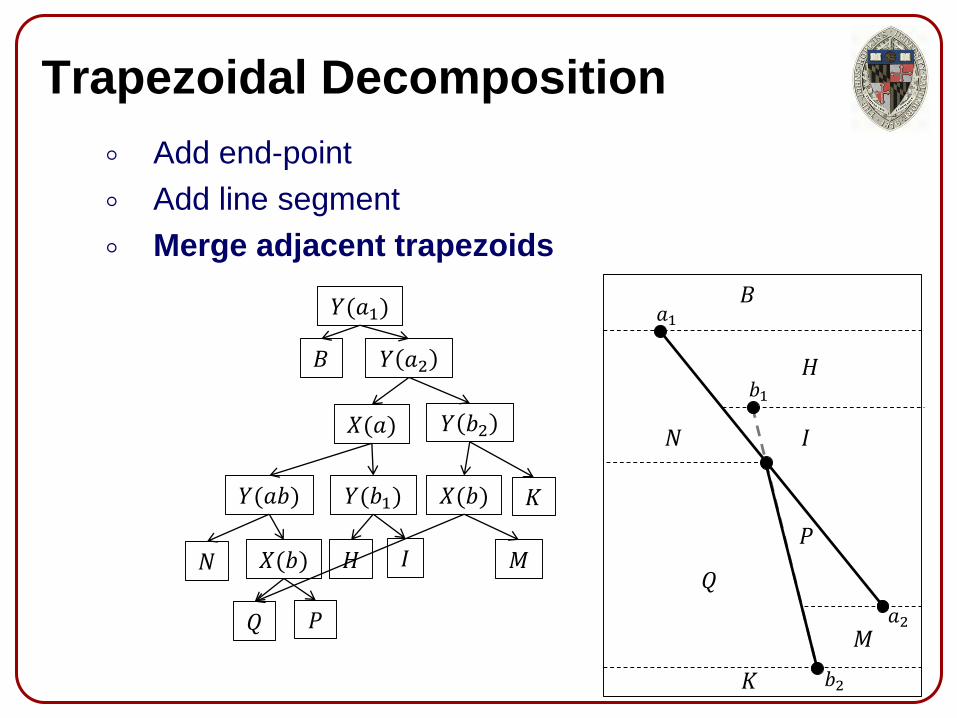
Add end-point
Add line segment
Merge adjacent trapezoids
Trapezoidal Decomposition
𝐵
𝐿
𝐼𝑁
𝐻
𝐾
𝑀
𝑂 𝑃
𝑎1
𝑏1
𝑎2
𝑏2
𝑌(𝑎1)
𝐵 𝑌 𝑎2
𝑋(𝑎) 𝑌 𝑏2
𝑌(𝑎𝑏) 𝑌(𝑏1)
𝐻 𝐼
𝑋(𝑏) 𝐾
𝑀𝑁 𝑋(𝑏)
𝑂 𝑃
𝐿
Add end-point
Add line segment
Merge adjacent trapezoids
Trapezoidal Decomposition
𝐵
𝐼𝑁
𝐻
𝐾
𝑀
𝑄
𝑃
𝑎1
𝑏1
𝑎2
𝑏2
𝑌(𝑎1)
𝐵 𝑌 𝑎2
𝑋(𝑎) 𝑌 𝑏2
𝑌(𝑎𝑏) 𝑌(𝑏1)
𝐻 𝐼
𝑋(𝑏) 𝐾
𝑀𝑁 𝑋(𝑏)
𝑄 𝑃

Add end-point
Add line segment (3)
Merge adjacent trapezoids
Trapezoidal Decomposition
𝐵
𝐼𝑁
𝐻
𝐾
𝑀
𝑄
𝑃
𝑎1
𝑏1
𝑎2
𝑏2
𝑌(𝑎1)
𝐵 𝑌 𝑎2
𝑋(𝑎) 𝑌 𝑏2
𝑌(𝑎𝑏) 𝑌(𝑏1)
𝐻 𝐼
𝑋(𝑏) 𝐾
𝑀𝑁 𝑋(𝑏)
𝑄 𝑃

Add end-point
Add line segment (3)
Merge adjacent trapezoids
Trapezoidal Decomposition
𝑎1𝑌(𝑎1)
𝐵
𝐵 𝑌 𝑎2
𝑋(𝑎) 𝑌 𝑏2 𝑇𝑁
𝑌(𝑎𝑏) 𝑌(𝑏1)
𝑏1
𝐻
𝐻 𝑌(𝑎𝑏)
𝑋(𝑏) 𝐾
𝐾
𝑀
𝑀
𝑁 𝑋(𝑏)𝑄
𝑄 𝑃
𝑃
𝑋(𝐵) 𝑅
𝑅
𝑆 𝑇
𝑆
𝑎2
𝑏2

Because of merging, we can have multiple paths
into the same trapezoid.
Trapezoidal Decomposition
𝑎1𝑌(𝑎1)
𝐵
𝐵 𝑌 𝑎2
𝑋(𝑎) 𝑌 𝑏2 𝑇𝑁
𝑌(𝑎𝑏) 𝑌(𝑏1)
𝑏1
𝐻
𝐻 𝑌(𝑎𝑏)
𝑋(𝑏) 𝐾
𝐾
𝑀
𝑀
𝑁 𝑋(𝑏)𝑄
𝑄 𝑃
𝑃
𝑋(𝐵) 𝑅
𝑅
𝑆 𝑇
𝑆
𝑎2
𝑏2

Because of merging, we can have multiple paths
into the same trapezoid.
Trapezoidal Decomposition
𝑎1𝑌(𝑎1)
𝐵
𝐵 𝑌 𝑎2
𝑋(𝑎) 𝑌 𝑏2 𝑇𝑁
𝑌(𝑎𝑏) 𝑌(𝑏1)
𝑏1
𝐻
𝐻 𝑌(𝑎𝑏)
𝑋(𝑏) 𝐾
𝐾
𝑀
𝑀
𝑁 𝑋(𝑏)𝑄
𝑄 𝑃
𝑃
𝑋(𝐵) 𝑅
𝑅
𝑆 𝑇
𝑆
𝑎2
𝑏2
Assuming the tree stays balanced, construction has complexity
𝑂((𝑛 + 𝑘) log 𝑛) and query has complexity 𝑂(log 𝑛) .
If line segments are added in random order , the tree
will be well-balanced, with high probability.

Outline
• Trapezoidal Decomposition
• Extreme Points (2D)
• Extreme Points (3D)
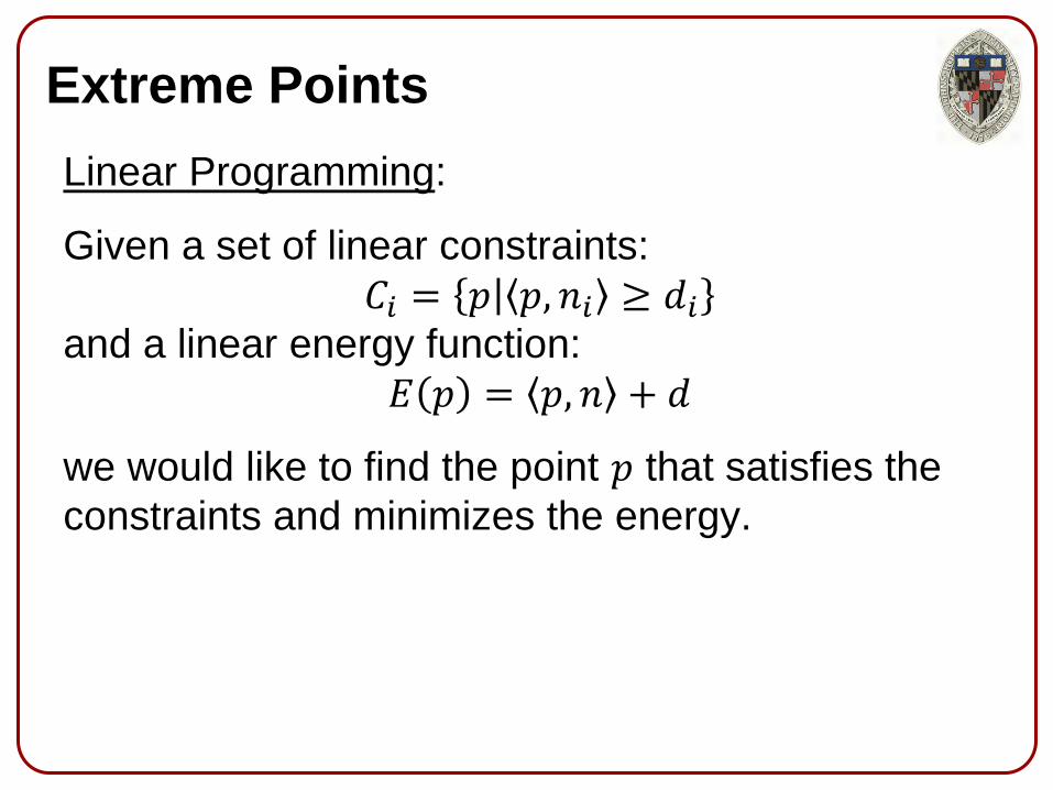
Extreme Points
Linear Programming:
Given a set of linear constraints:
𝐶𝑖 = 𝑝 𝑝, 𝑛𝑖 ≥ 𝑑𝑖
and a linear energy function:
𝐸 𝑝 = 𝑝, 𝑛 + 𝑑
we would like to find the point 𝑝 that satisfies the
constraints and minimizes the energy.

Extreme Points
Linear Programming: Since the constraints are linear, each one defines a
half-space of valid solutions.
The intersection of these
half-spaces is convex.
Since the energy is
linear, it has a constant
gradient 𝛻𝐸 pointing
away from the minimum.
The minimizer is the point
in the convex region which
is extreme along direction 𝑛.
𝛻𝐸

Extreme Points (2D)
Given a convex polygon 𝑃, we would like to find the
extreme points along a particular direction.
Without loss of generality, we can assume that the
direction is vertical.
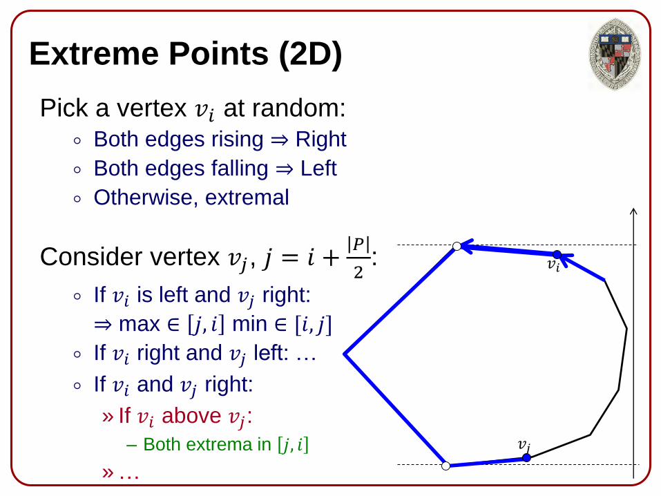
Extreme Points (2D)
Pick a vertex 𝑣𝑖 at random: Both edges rising ⇒ Right
Both edges falling ⇒ Left
Otherwise, extremal
Consider vertex 𝑣𝑗, 𝑗 = 𝑖 +𝑃
2:
If 𝑣𝑖 is left and 𝑣𝑗 right:
⇒ max ∈ 𝑗, 𝑖 min ∈ [𝑖, 𝑗]
If 𝑣𝑖 right and 𝑣𝑗 left: …
If 𝑣𝑖 and 𝑣𝑗 right:
» If 𝑣𝑖 above 𝑣𝑗:– Both extrema in 𝑗, 𝑖
» …
𝑣𝑖
𝑣𝑗
With repeated bisection, we can find
the two extrema in 𝑂(log 𝑃 ) time.
Outline
• Trapezoidal Decomposition
• Extreme Points (2D)
• Extreme Points (3D)

Extreme Points (3D)
Given a convex polyhedron 𝑃, we would like to find
the (without loss of generality) highest point.
[Kirkpatrick, 1983]
Compute a hierarchy of nested polytopes, compute
the highest point on the coarsest polytopes and use
that to efficiently compute the highest point on the
next polytope.
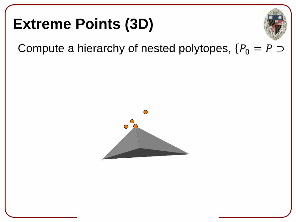
Compute a hierarchy of nested polytopes, 𝑃0 = 𝑃 ⊃
Extreme Points (3D)

Definition:
Given a graph, a set of vertices is said to be
independent if there is no edge in the graph that
connects vertices in the set.
Key Idea:
Identify an independent set of vertices
on 𝑃𝑘 with low degree, remove
those, and set 𝑃𝑘+1 to the
convex hull of what’s left.
Repeat for subsequent levels of the hierarchy.
Constructing the Hierarchy
Greedy Algorithm:
• While not done Find a vertex with degree ≤ 8.
If none of its neighbors have been marked as
independent, mark it as independent.
Claim:
This algorithm will mark a at least 1/18 of the
vertices as independent.
Constructing the Hierarchy

Proof:
By Euler’s formula, for a triangulated polyhedron:
𝐸 = 3𝑉 − 6.
⇒ The sum of the degrees of the vertices, Σ, is
equal to twice the number of edges, and hence:
Σ = 6𝑉 − 12.
⇒ There are at least 𝑉/2 vertices with degree ≤ 8.
Otherwise, there are at least 𝑉/2 vertices with
degree ≥ 9 and the rest have degree at least 3:
Σ ≥9𝑉
2+
3𝑉
2= 6𝑉 > 6𝑉 − 12 = Σ (⇒⇐)
Constructing the Hierarchy

Proof:
There are at least 𝑉/2 vertices with degree ≤ 8.
⇒ Marking a low-degree vertex as independent, we
invalidate (at most) 8 other vertices.
⇒ Repeating, we will mark at least 1/9 of the low-
degree vertices as independent
⇒ 1/18 of all vertices will be independent.
Constructing the Hierarchy
Using this to construct our polytope hierarchy:
• We will have 𝑂(log |𝑃|) levels.
• We will require 𝑂(|𝑃|) storage.

Claim:
If we remove a point on a polytope, the convex hull
of the remaining points can be obtained by
computing the convex hull of the points on the
boundary and using the “outer” half of the triangles.
Proof:
The remaining triangles must still be on the hull.
Any new triangles can’t connect to non-boundary
vertices because then the hull would be non-
manifold.
Constructing the Hierarchy
Since the removed vertices are independent and have
degree ≤ 8, the coarser convex hull can be computed in
time proportional to the number of removed points.
Since a removed vertex does not appear later
on in the hierarchy, the complexity of
computing the hierarchy is 𝑂 |𝑃| .

Claim:
After remove the highest vertex 𝑣 ∈ 𝑃, the next
highest vertex 𝑤 has to be in the one-ring of 𝑣.
Proof: (by contradiction)
Assume 𝑤 is interior.
⇒ The closed loop of neighbors
of 𝑤 are below 𝑤.
⇒ 𝑃 must be below the cone apexed
at 𝑤 and going through its neighbors.
⇒ 𝑤 was above 𝑣. (⇒⇐)
Constructing the Hierarchy
𝑣
Given the highest vertex, 𝑣𝑘+1 ∈ 𝑃𝑘+1 the highest
vertex 𝑣𝑘 ∈ 𝑃𝑘 is either 𝑣𝑘+1 or is in its one-ring.
We can’t test all neighbors of 𝑣𝑘+1
because 𝑣𝑘+1 may have large degree!

Definition:
An edge 𝑒 on 𝑃𝑘+1 is exposed by a vertex 𝑝 ∈ 𝑃𝑘, if
𝑒 is in the triangulation of the hole resulting from the
removal of 𝑝.
Constructing the Hierarchy

Definition:
An edge 𝑒 on 𝑃𝑘+1 is exposed by a vertex 𝑝 ∈ 𝑃𝑘, if
𝑒 is in the triangulation of the hole resulting from the
removal of 𝑝.
Constructing the Hierarchy
An edge 𝑒 ⊂ 𝑃𝑘+1 is exposed by 𝑝 ∈ 𝑃𝑘
if 𝑒 is visible to 𝑝 when viewing 𝑃𝑘+1.
An edge in 𝑃𝑘+1 can be exposed by at most two vertices.
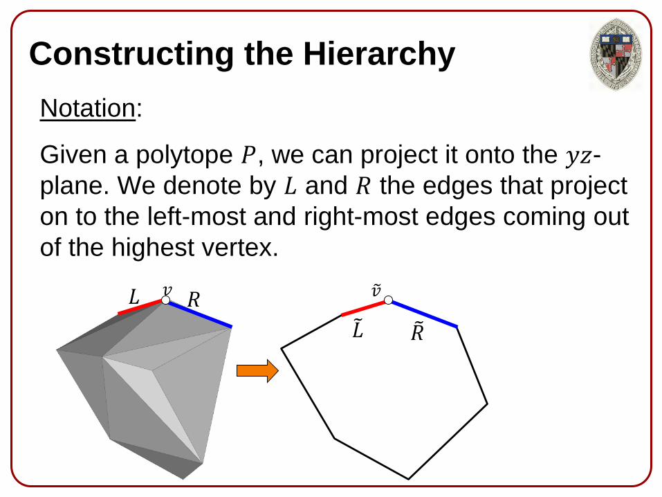
Notation:
Given a polytope 𝑃, we can project it onto the 𝑦𝑧-
plane. We denote by 𝐿 and 𝑅 the edges that project
on to the left-most and right-most edges coming out
of the highest vertex.
Constructing the Hierarchy
𝑅 𝐿
𝑣𝑅𝐿 𝑣

Claim:
Given the highest vertex, 𝑣𝑘+1 ∈ 𝑃𝑘+1 the highest
vertex 𝑣𝑘 ∈ 𝑃𝑘 is either 𝑣𝑘+1, or the vertex that
exposes one of 𝐿𝑘+1 and 𝑅𝑘+1.
Constructing the Hierarchy
𝑅𝑘+1 𝐿𝑘+1
𝑣𝑘+1
𝑣𝑘𝑣𝑘
𝑣𝑘+1𝑅𝑘+1𝐿𝑘+1

Proof: Draw triangles (𝑣𝑘 , 𝐿𝑘+1) and (𝑣𝑘 , 𝑅𝑘+1).
One of these cannot intersect 𝑃𝑘+1
(otherwise its projection would intersect).
⇒ One of 𝐿𝑘+1 or 𝑅𝑘+1 is exposed by 𝑣𝑘.
Constructing the Hierarchy
𝑣𝑘 𝑣𝑘
𝑣𝑘+1𝐿𝑘+1
𝑣𝑘
𝑅𝑘+1 𝐿𝑘+1
𝑣𝑘+1𝑅𝑘+1

Proof: Draw triangles (𝑣𝑘 , 𝐿𝑘+1) and (𝑣𝑘 , 𝑅𝑘+1).
One of these cannot intersect 𝑃𝑘+1
(otherwise its projection would intersect).
⇒ One of 𝐿𝑘+1 or 𝑅𝑘+1 is exposed by 𝑣𝑘.
Constructing the Hierarchy
𝑣𝑘 𝑣𝑘
𝑣𝑘+1𝐿𝑘+1
𝑣𝑘
𝑅𝑘+1 𝐿𝑘+1
𝑣𝑘+1𝑅𝑘+1
If we know the highest vertex 𝑣𝑘+1 ∈ 𝑃𝑘+1 and
we know 𝐿𝑘+1 and 𝑅𝑘+1, then we get the
highest vertex 𝑣𝑘 ∈ 𝑃𝑘 in 𝑂(1).
If 𝑣𝑘+1 is removed at level 𝑘 + 2:
⇒ 𝑣𝑘+1 has degree ≤ 8⇒ We can find 𝐿𝑘+1 and 𝑅𝑘+1 with exhaustive search.
Otherwise, we can use 𝐿𝑘+2 and 𝑅𝑘+2 to compute 𝐿𝑘+1
and 𝑅𝑘+1 in time 𝑂(1).
• We can construct the polytope hierarchy in 𝑂 𝑃 time.
• We can find the extreme point, with respect to an
arbitrary direction, in 𝑂 log 𝑃 .


