WP/13/232
Rules of Thumb for
Bank Solvency Stress Testing
Daniel C. Hardy and Christian Schmieder
© 2010 International Monetary Fund WP/13/232
IMF Working Paper
Monetary and Capital Markets Departments
Rules of Thumb for Bank Solvency Stress Testing
Prepared by Daniel C. Hardy and Christian Schmieder1
Authorised for distribution by Daniel C. Hardy
November 2013
Abstract
This Working Paper should not be reported as representing the views of the IMF.
The views expressed in this Working Paper are those of the author(s) and do not necessarily represent
those of the IMF/BIS/BCBS or IMF/BIS/BCBS policy. Working Papers describe research in progress by
the author(s) and are published to elicit comments and to further debate.
Rules of thumb can be useful in undertaking quick, robust, and readily interpretable bank
stress tests. Such rules of thumb are proposed for the behavior of banks’ capital ratios and
key drivers thereof—primarily credit losses, income, credit growth, and risk weights—in
advanced and emerging economies, under more or less severe stress conditions. The
proposed rules imply disproportionate responses to large shocks, and can be used to
quantify the cyclical behaviour of capital ratios under various regulatory approaches.
JEL Classification Numbers: G21, G28, G32
Keywords: Stress testing, rules of thumb, bank stability, bank capitalization
Author’s E-Mail Address: [email protected] , [email protected]
1 International Monetary Fund, and Basel Committee on Banking Supervision, Bank for International
Settlements, respectively. The authors would like to thank Martin Čihák, Sam Langfield, Li Lian Ong, and
Mario Quagliariello for helpful comments and suggestions.
2
Contents Page
I. Introduction ............................................................................................................................4
II. Methodology and Sources .....................................................................................................8
III. Typical Banking Crises and Descriptive Rules of Thumb .................................................11
A. Literature on Banking Crises ...........................................................................11 B. Historical Evidence on Banking Crises ...........................................................14 C. Descriptive Rules of Thumb ............................................................................17
IV. Rules of Thumb for Satellite Models.................................................................................29
A. Explanatory Variables and Estimation Approach ............................................30 B. Rules of Thumb for Satellite Models ...............................................................33
V. Worked Examples ...............................................................................................................42 A. Bank Characteristics ........................................................................................42
VI. Conclusion .........................................................................................................................53
Appendix 1. Data Summary .....................................................................................................56
Appendix 2. Supplementary Evidence .....................................................................................59
References ................................................................................................................................64
Tables
1. Čihák and Schaeck Evidence on Typical Evolution of NPL Stock Ratios Around a
Crisis ........................................................................................................................................12
2. Typical Credit Loss Levels under Different Levels of Shocks ............................................17
3. Stress Levels of Default Rates and LGDs for ACs ..............................................................21
4. Rules of Thumb for the GDP Sensitivity of Key Bank Solvency Variables .......................34
5. Historical Evidence on Typical Evolution of Default Dates Around a Crisis .....................36
6. Rules of Thumb for the GDP Growth Sensitivity of Credit Risk Parameters .....................37
7. Features of Banks Used in the Worked Examples ...............................................................43
8. Simulated Evolution of RWAs Relative to Total Assets During Stress Periods .................46
9. Simulated Evolution of Net Income during Stress Periods .................................................48
10. Overview of Main Rules of Thumb ...................................................................................53
Figures
1. Čihák and Schaeck Evidence on Typical Evolution of NPL Ratios Around a Crisis..........12
2. Historical Annual Default Rate for All Rating Grades ........................................................15
3. Historical Corporate Bond Default Rates (1866–2008) .......................................................16
4. Median Loss Rates by Country (1996–2011) ......................................................................18
5. Typical Evolution of Credit Loss Rates under Stress ..........................................................19
6. Evolution of LGDs through the cycle ..................................................................................20

3
7. Link Between LGDs and Default Rates...............................................................................21
8. Typical Evolution of Pre-impairment Income Under Stress................................................24
9. Evolution of Pre-impairment Income for Worst Performing Banks under Stress ...............25
10. Standard Deviation Across Crisis Periods of Median Income and Expense
Components .............................................................................................................................26
11. Trading Income under Stress, by Quantile ........................................................................27
12. Typical Evolution of Credit Growth for ACs and EMs under Stress ................................29
13. Historical Evidence on Typical Evolution of Default Rates Around a Crisis ...................36
14a. Comparison Between IRB Asset Correlation and Empirical Asset Correlations for
Corporate Debt .........................................................................................................................41
14b. Resulting Risk Weights....................................................................................................41
15. Evolution of Capital Ratios during Stress Periods .............................................................44
16. Evolution of Leverage Ratios during Stress Periods .........................................................47
17. Evolution of Capital Ratios: Actual vs. Predicted for an AC Bank ...................................49
18. Capital Ratios with Point-In-Time vs. Through-The-Cycle RWAs ..................................52
Boxes
1. Proxies for Credit Loss Rates ..............................................................................................14
2. How Likely is it that Large Trading Losses Coincide with Large Credit Losses? ..............28
3. How do IRB Correlations Compare with Empirical Correlations? .....................................40
4. Rules of Thumb Applied to Recent Stress Tests .................................................................50
Appendixes
1. Data Summary .....................................................................................................................56
2. Supplementary Evidence .....................................................................................................59
Appendix Tables
1 Overview of Bankscope Data ...............................................................................................56
2. Overview of Top 10 Countries by Category for Cleaned Bankscope Data .........................57
3. Overview of Bankscope Data, by Stress Level ....................................................................58
4. Evolution of Solvency Parameters around Crisis Dates ......................................................59
5. Components of Pre-impairment Income and Expenses .......................................................61
Appendix Figures
1 Overview of Raw Bankscope Sample Size by Year .............................................................56
2. Asset Correlations ................................................................................................................63
3. Asset Correlations and GDP Growth Rates .........................................................................63
4
I. INTRODUCTION
Financial sector stress testing has become a widespread, important, and prominent
activity. Stress testing is used to identify financial sector vulnerabilities, 2 to inform policy
decisions affecting the financial system and individual institutions,3 and to guide
companies’ own risk management. Yet, its practical application is often demanding, and
there remain questions about its reliability.
Obtaining stress test results and establishing their robustness would be facilitated by the
availability of “rules of thumb,” that is, rough guides to typical behavioral relationships,
magnitudes of shocks, and the impact of shocks on banks, based on a wide range of
experience. This paper attempts identifying such rules of thumb that apply to bank
solvency, that is, capital ratios. The rules of thumb elaborated in this study are meant to
serve mainly as general guidelines, particularly to understand worst-case scenarios, and
to complement rather than substitute for detailed analysis of a country’s banks and its
institutional, financial and conjunctural circumstances.
Rules of thumb would be useful at various stages of stress testing:
One challenge is to design tests for a country with limited relevant experience and
data, either because of structural breaks in time series or because the county did
not suffer a severe banking crisis in recent decades. Then, on the one hand, rules
of thumb derived from experience in various countries with underlying
similarities can be used to construct and calibrate relevant stress tests for the
country concerned. Rules of thumb based on long, world-wide experience provide
indicators of the great variety of scenarios that countries have suffered. On the
other hand, given a scenario, rules of thumb for behavioral relationships can be
used to make projections when reliable stress testing methods are unavailable
locally. For example, when national authorities or bank management are unable to
estimate behavioral relationships robustly based on the data available, it may be
wise to “import” a rule of thumb.
Even when national experience and data allow the construction of a relatively
complex model that captures well past behavior, it could be less relevant in the
future (for example, because certain asset classes are more or less relevant than
they were in the past), and thus give a false sense of accuracy; “model
uncertainty” is an important consideration in stress testing and risk management
2 For example, macro stress tests as part of Financial Sector Assessment Programs (Jobst, 2013).
3 Examples are the U.S. regulatory stress tests conducted in 2009 (Supervisory Capital Assessment
Program, SCAP) and 2012 (Comprehensive Capital Analysis and Review, CCAR) and the European Stress
Tests conducted in 2010 and 2011 by the European Banking Authority (EBA).
5
more generally, though it is easy to overlook. Unless one knows with some
precision the behavioral relationships that are relevant going forward, a simple
rule of thumb may provide the most reliable estimates and basis for action
(Haldane, 2012 and 2013). Rules of thumb can be used also to check the
plausibility of estimates of behavior derived from national experience.
It is often important to assess, and if possible quantify, the potential impact of
nonlinearities; stress tests are much more informative and credible if one can say
how sensitive are results to changes in assumptions (Taleb et al, 2012). To this
end, the ability to conduct multiple “runs” at low marginal cost using rules of
thumb, rather than re-analyzing data in fine detail, is valuable to supervisors and
managers.
Rules of thumb can be used to assess the stability implications of various
prudential rules, such as minimum capital requirements, including on a cross-
country basis. With rules of thumb, one can generate rough projections of the
magnitude of shocks that banks typically face and what they could withstand
depending on their capitalization and other characteristics. Such projections
would not replace detailed impact studies, but would provide a plausibility and
robustness check.
Stress test frameworks (methods and assumptions alike) and outcomes have to be
readily accessible for senior managers and policy-makers if action is to be
triggered. A very complex model may be difficult to interpret and to link to policy
instruments, and therefore it may distract from an informed debate on what
actions should be taken; debate over the model may obscure debate over policy.
To this end, decision-makers would be helped by the availability of readily
understandable benchmarks regarding the potential outcome of stress tests and
some of the main behavioral relationships underlying them.
Motivated by on these considerations, this paper concentrates on the formulation of rules
of thumb for key factors affecting bank solvency, namely credit losses, pre-impairment
income and credit growth during crises, and illustrates their use in the simulation of the
evolution of capital ratios under stress.4 We thereby seek to provide answers to the
following common questions in stress testing:
How much do credit losses usually increase in case of a moderate, medium and
severe macroeconomic downturn and/or financial stress event, e.g., if cumulative
4 Effects of managerial action such as the raising of capital, asset disposals, and balance sheet restructuring,
and those of structural changes such as exit of firms, are not analyzed here, in keeping with standard
methodology of stress testing.

6
real GDP growth turns out to be, say, 4 or 8 percentage points below potential (or
average or previous years’) growth?
How typically do other major factors that affect capital ratios, such as
profitability, credit growth, and risk-weighted assets (RWA), react under these
circumstances?
Taking these considerations together, how does moderate, medium, or severe
macro-financial stress translate into (a decrease in) bank capital, and thus, how
much capital do banks need to cope with different levels of stress?
In answering these sorts of questions, a useful set of rules of thumb for stress testing
should embody several properties:
Coverage of the major factors contributing to banks’ vulnerabilities (in terms of
solvency).
Wide applicability, but with criteria to determine where inapplicable. A rule of
thumb should be useful in many circumstances and many countries, but it should
be clear where it should not be used.
Robustness, implying that the rule is supported by a variety of evidence and not
subject to excessive model risk.
Intuitiveness, so that it can be used to interpret results and inform decision-
making.
As a corollary of these properties, a desirable rule of thumb should be relatively simple.
Simplicity is likely to enhance wide applicability, robustness, and intuitiveness. Rules
will be developed along these principles.
To find common patterns, the study investigated various pieces of empirical evidence,
including descriptive statistics, which may capture stress that does not necessarily
originate from measured macroeconomic factors. Our analysis includes data from various
previous crises, but focuses on the crises during the last 15 years (including the
Russian/Asian crisis, crises experienced by the transition countries in Central and Eastern
Europe in the late 1990s, the burst of the internet bubble in the early 2000s, the global
financial crisis, and country, as well as bank-specific crises).
The evidence justifies distinguishing between emerging market economies (EMs) and
advanced economies (ACs), because their typical behavior differs importantly.5 These
5 Distinguish between advanced, emerging market, and low income countries is common practice in
academic literature (such as Hardy and Pazarbasioglu, 1999), and policy-oriented analysis (such as the
(continued…)
7
differences can plausibly be attributed to differences in macroeconomic performance—
for example, EMs tend to have relatively large cyclical fluctuations—and structural
factors, such as the effectiveness of loan workout mechanisms. Because the rules of
thumb differ across ACs and EMs, as do the typical magnitudes of shocks, different
levels of capitalization are needed to achieve a given level of resilience against potential
shocks. Evidence from low income countries (LICs) is used whenever possible, but less
is available, and the functioning of LIC economies may differ from that of both ACs and
EMs, for example, because of greater dependence on export of commodities and a much
lower level of bank intermediation.
The evidence suggests also that the behavior of relevant variables (loss rates, income,
credit growth, RWAs, capital ratios) is highly non-linear around crises. Effects on bank
capitalization and loan quality under a severe crisis are disproportionately great. In case
of credit losses, for example, severe loss levels are many times higher than in normal
times, and in such circumstances banks typically exhibit substantially lower pre-
impairment income that can be used as a buffer against losses. In response to stresses,
they restrain from paying dividend and/or deleverage, the latter being a powerful way to
restore bank solvency but a macroeconomically costly alternative if it comes along with
constrained credit supply.
It is found also that the interpretation of capital levels should take into account
differences in the measurement of regulatory capital: the measured risk-based
capitalization of a bank using the standardized approach (StA) under the Basel II standard
will be less sensitive to both positive and negative shocks than that of a bank using the
Internal Ratings-Based approach (IRB). On this basis, one may suggest that the StA may
be slow to reveal emerging vulnerabilities, while the IRB approach more quickly reflects
deterioration in a bank’s situation (and rebounds faster when conditions improve),
provided that changes in risk are reflected in IRB risk weights on a timely basis.6 By the
same token, a given level of risk-based capitalization during benign times may be less of
a buffer for a bank using the IRB approach than for a bank using the StA.
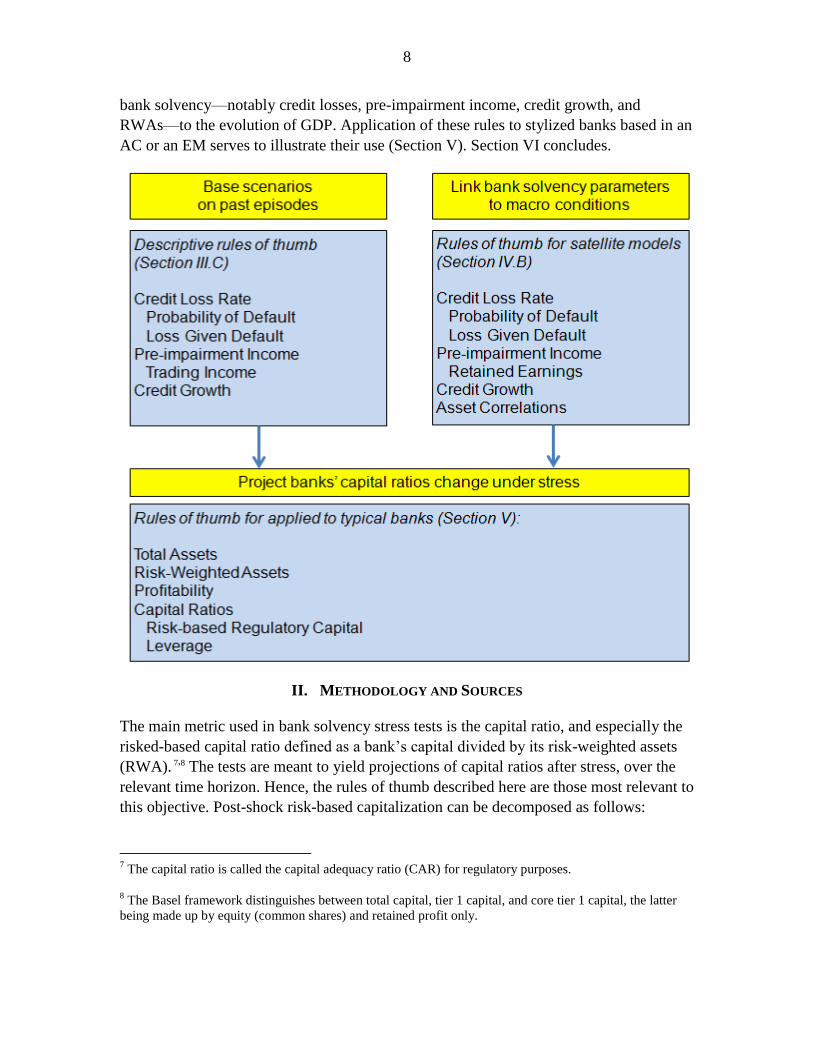
The structure of the paper and the main variables investigated are illustrated in the
following chart. Section II explains the main elements of the approach and the evidence
available. Section III contains the proposed descriptive rules of thumb based on stylized
facts of financial crises, where the rules are conditional on the evolution of credit losses.
Section IV contains rules of thumb versions of satellite models that link the key drivers of
IMF’s Global Financial Stability Reports), in recognition of the important differences among them in terms
of economic institutions, trends, and vulnerabilities.
6 The risk sensitivity of RWAs under the IRB depends on the degree to which a bank’s rating system is
based on “point-in-time” (PIT) rather than “through-the-cycle” (TTC) parameters.
8
bank solvency—notably credit losses, pre-impairment income, credit growth, and
RWAs—to the evolution of GDP. Application of these rules to stylized banks based in an
AC or an EM serves to illustrate their use (Section V). Section VI concludes.
II. METHODOLOGY AND SOURCES
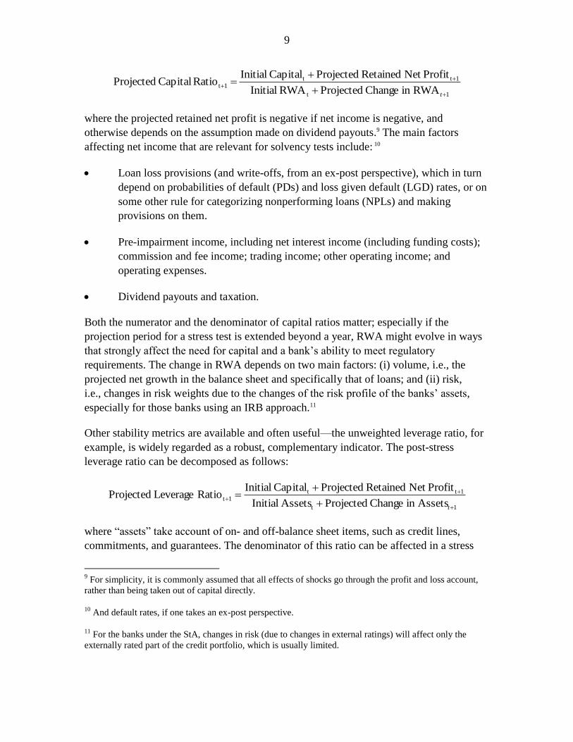
The main metric used in bank solvency stress tests is the capital ratio, and especially the
risked-based capital ratio defined as a bank’s capital divided by its risk-weighted assets
(RWA). 7,8 The tests are meant to yield projections of capital ratios after stress, over the
relevant time horizon. Hence, the rules of thumb described here are those most relevant to
this objective. Post-shock risk-based capitalization can be decomposed as follows:
7 The capital ratio is called the capital adequacy ratio (CAR) for regulatory purposes.
8 The Basel framework distinguishes between total capital, tier 1 capital, and core tier 1 capital, the latter
being made up by equity (common shares) and retained profit only.
9
1t
1tt1t
RWAin Change ProjectedRWA Initial
ProfitNet Retained ProjectedCapital InitialRatio Capital Projected
t
where the projected retained net profit is negative if net income is negative, and
otherwise depends on the assumption made on dividend payouts.9 The main factors
affecting net income that are relevant for solvency tests include: 10
Loan loss provisions (and write-offs, from an ex-post perspective), which in turn
depend on probabilities of default (PDs) and loss given default (LGD) rates, or on
some other rule for categorizing nonperforming loans (NPLs) and making
provisions on them.
Pre-impairment income, including net interest income (including funding costs);
commission and fee income; trading income; other operating income; and
operating expenses.
Dividend payouts and taxation.
Both the numerator and the denominator of capital ratios matter; especially if the
projection period for a stress test is extended beyond a year, RWA might evolve in ways
that strongly affect the need for capital and a bank’s ability to meet regulatory
requirements. The change in RWA depends on two main factors: (i) volume, i.e., the
projected net growth in the balance sheet and specifically that of loans; and (ii) risk,
i.e., changes in risk weights due to the changes of the risk profile of the banks’ assets,
especially for those banks using an IRB approach.11
Other stability metrics are available and often useful—the unweighted leverage ratio, for
example, is widely regarded as a robust, complementary indicator. The post-stress
leverage ratio can be decomposed as follows:
1t
1tt1t
Assetsin Change ProjectedAssets Initial
ProfitNet Retained ProjectedCapital InitialRatio Leverage Projected
t
where “assets” take account of on- and off-balance sheet items, such as credit lines,
commitments, and guarantees. The denominator of this ratio can be affected in a stress
9 For simplicity, it is commonly assumed that all effects of shocks go through the profit and loss account,
rather than being taken out of capital directly.
10 And default rates, if one takes an ex-post perspective.
11 For the banks under the StA, changes in risk (due to changes in external ratings) will affect only the
externally rated part of the credit portfolio, which is usually limited.

10
scenario if allowance is made for on- and off-balance sheet growth, including through the
write-off of losses. Factors affecting the numerator are the same as those for the risk-
based capital ratio.
Return on capital (ROC) and return on assets are indicative of a bank’s ability to recover
from a capital loss. Indeed, profitability is the first line of defense of any bank against
credit and other risk. A sufficiently profitable bank can earn enough to restore its
capitalization even in the face of substantial stress, either by attracting new capital with
the promise of dividends or by retaining earnings. A bank with low profitability will be
less able to recover from even a brief negative shock. The proposed rules of thumb are
useful for projecting these metrics as well.
The rules of thumb are derived from the literature on banking crises, and statistical
evidence on the evolution of bank loan quality and quantity obtained from two datasets:
Long-sample evidence is provided by data on default rates over a period of
90 years (1920–2012) for ACs, and indeed mainly U.S. corporates (Moody’s
2013).12, 13 Specifically, Moody’s reports annual exposure-weighted historical
default rates. This long sample includes five periods of substantial stress.
Recent cross-country evidence is provided by data on the sample of banks
available in Bankscope. The time dimension is limited to the period from 1996 to
2011, with the number of banks increasing in the later part of the sample.
However, this period does cover various episodes of stress in the countries
covered. Evidence is obtained on bank performance in ACs, EMs and some LICs.
The data covers more than 16,000 banks in 200 countries and jurisdictions, but the
majority of banks (more than 13,000) are based in ACs (almost half in the United
States), about 3,000 in are EMs, and only 550 are in LICs. There is some selection
bias toward larger banks, especially in the LICs, which renders the evidence for
these countries less robust. For the establishment of the rules of thumb, outliers
were removed from the sample to avoid misleading results, and other robustness
checks were performed, leaving a sample of more than 10,000 banks from almost
170 countries.14 Summary statistics are provided in Appendix 1.
12
The majority of counterparts rated by Moody’s are based in the United States, especially in the earlier
part of the sample.
13 This database is the longest readily available and relevant time series for bank solvency research.
14 Data for some banks’ solvency variables contain numerous missing values. All banks with less than
5 observations overall (during 1996–2011) were excluded from the sample. Very high loss levels (even
above 100 percent) were observed for a few banks, for example, because of substantial off-balance sheet
credit operation. Such outliers were removed from the sample.

11
Such evidence drawn from a wide range of times and countries no doubt suffers from
large differences in definitions of relevant variables, and the analysis of the evidence
needs to recognize and cope with this challenge. Even today among countries using
accounts based on International Financial Reporting Standards, criteria for classifying
assets or defining capital, for example, can differ widely. Loss recognition and
provisioning practices can differ from bank to bank within the same jurisdiction. Yet, for
the purposes of this study, using a wide range of evidence is essential: only diverse data
sources can yield evidence on the effects of extreme but plausible shocks, including
shocks which force banks to reveal losses that are hidden in normal times. An attempt is
made to limit the influence of data problems by using relatively robust techniques, and
also by looking at indicators of both location and spread.
III. TYPICAL BANKING CRISES AND DESCRIPTIVE RULES OF THUMB
A simple but possibly robust approach to defining and calibrating a stress test for a
banking crisis is to look at historical episodes, not just in one country—which may have
limited experience—but in a range of comparable countries. Past crises episodes and
severe recessions provide highly relevant information on the impact of stress on bank
solvency through various channels. In what follows we seek to come up with descriptive
rules of thumb, after some suggestive conclusions on the link between macroeconomic
conditions and banks’ performance.
A. Literature on Banking Crises
There is a large literature on banking crises, mostly looking at macroeconomic precursors
and effects, and at the effectiveness of the strategies adopted on different occasions.15 A
subset of studies provides quantitative evidence that is of direct relevance to stress
testing. One example thereof is Čihák and Schaeck (2007), who look at 51 episodes of
banking crisis during 1994–2004, in a sample that covers countries from every region.
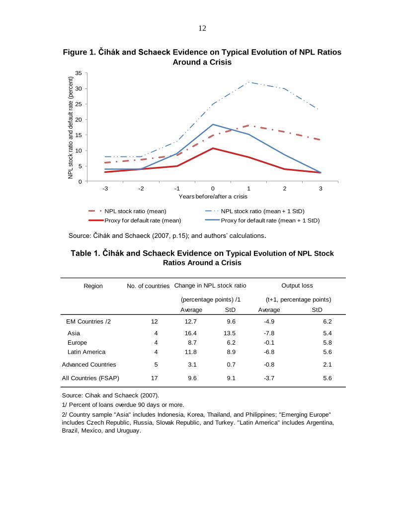
Figure 1 illustrates the typical behavior of default rates through a crisis, showing the
evolution of the stock and (a proxy for) the inflow of NPLs relative to total loans three
years on either side of a crises peak. Table 1 provides more detailed estimates, broken
down by region.
15
Lo (2012), for example, provides a recent overview of studies related to macroeconomic and financial
crises.
12
Figure 1. Čihák and Schaeck Evidence on Typical Evolution of NPL Ratios
Around a Crisis
Source: Čihák and Schaeck (2007, p.15); and authors’ calculations.
Table 1. Čihák and Schaeck Evidence on Typical Evolution of NPL Stock
Ratios Around a Crisis
0
5
10
15
20
25
30
35
-3 -2 -1 0 1 2 3
NP
L s
tock ratio
and d
efa
ult
rate
(perc
ent)
Years before/after a crisis
NPL stock ratio (mean) NPL stock ratio (mean + 1 StD)
Proxy for default rate (mean) Proxy for default rate (mean + 1 StD)
Region No. of countries
(percentage points) /1 (t+1, percentage points)
Average StD Average StD
EM Countries /2 12 12.7 9.6 -4.9 6.2
Asia 4 16.4 13.5 -7.8 5.4
Europe 4 8.7 6.2 -0.1 5.8
Latin America 4 11.8 8.9 -6.8 5.6
Advanced Countries 5 3.1 0.7 -0.8 2.1
All Countries (FSAP) 17 9.6 9.1 -3.7 5.6
Source: Cihak and Schaeck (2007).
1/ Percent of loans overdue 90 days or more.
Change in NPL stock ratio Output loss
2/ Country sample "Asia" includes Indonesia, Korea, Thailand, and Philippines; "Emerging Europe"
includes Czech Republic, Russia, Slovak Republic, and Turkey. "Latin America" includes Argentina,
Brazil, Mexico, and Uruguay.

13
It can be seen that NPL stock ratios (in many countries still the most commonly available
credit risk indicator) increase substantially during crises, and typically peak one year after
the materialization of a crisis.16 The temporal shift reflects the fact that some loans default
with some time lag after the materialization of macroeconomic stress, and that many
banks have tended to recognize NPLs with delay, i.e., do not provision fully all potential
losses after the first year(s) of a crisis.17,18 The NPL stock ratios rise by about
10 percentage points from the typical level one year before the crisis, in “average” crises,
and almost 25 percentage points in severe crises. The stock is persistent: even after three
years, the NPL ratio is at about the same level when the crisis materializes.
Using NPL flow ratios as a proxy for default rates (Box 1), we find that they peak at
about 10 percent in “average” crises, and at about 18 percent in severe crises, up from
3 percent in “normal” times. The evidence here suggests that default rates come down to
pre-crisis levels after three years, which makes their pattern roughly symmetric with
respect to the crisis. The time needed to resolve problem loans implies that reduction in
the stock tends to take longer.19
One immediate implication of this evidence by type of country is that the NPL ratio and
the NPL flow ratio in EMs tend to peak at higher levels, and are generally more variable
than those in ACs. Also, real GDP growth is much more variable in EMs. A useful set of
rules of thumb need to accommodate these major differences; different rules may be
needed for ACs and EMs. Similarly large differences in typical behavior across types of
country will be documented in the analysis that follows.
16
The NPL stock ratio does not provide information on flows of credit losses, but proxies’ cumulative
default rates less write-offs.
17 Insofar as a banking crisis is preceded by rapid credit growth, many credits do not mature until after the
peak of the crisis.
18 Fair value accounting and risk-based capitalization (under Basel II) is meant to remove the opaqueness of
banks. Yet, regulatory rules are meant to follow a through-the-cycle approach, mitigating pro-cyclicality.
For stress testing purposes, point-in-time information is needed to monitor the current state of bank
solvency. See the discussion in Section V.
19 In case of less severe crises, the default rate is close to the long-term average already two years after the
trough of the crisis.
14
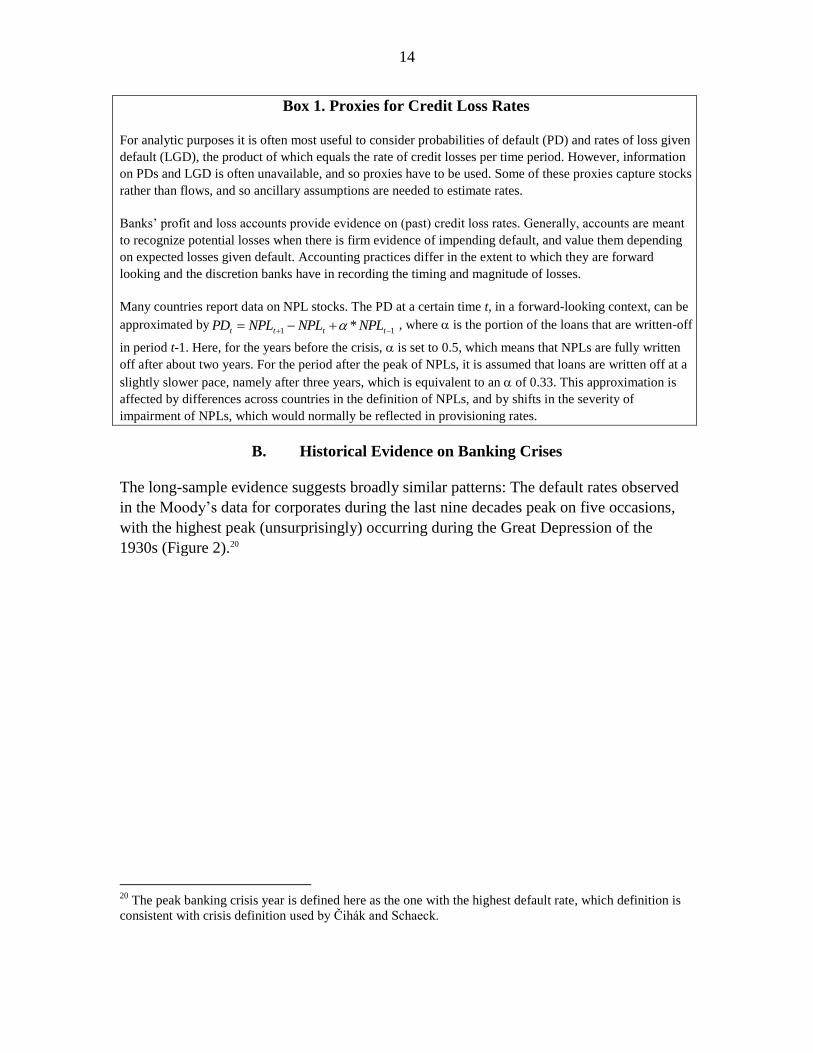
Box 1. Proxies for Credit Loss Rates
For analytic purposes it is often most useful to consider probabilities of default (PD) and rates of loss given
default (LGD), the product of which equals the rate of credit losses per time period. However, information
on PDs and LGD is often unavailable, and so proxies have to be used. Some of these proxies capture stocks
rather than flows, and so ancillary assumptions are needed to estimate rates.
Banks’ profit and loss accounts provide evidence on (past) credit loss rates. Generally, accounts are meant
to recognize potential losses when there is firm evidence of impending default, and value them depending
on expected losses given default. Accounting practices differ in the extent to which they are forward
looking and the discretion banks have in recording the timing and magnitude of losses.
Many countries report data on NPL stocks. The PD at a certain time t, in a forward-looking context, can be
approximated by11 * tttt NPLNPLNPLPD , where is the portion of the loans that are written-off
in period t-1. Here, for the years before the crisis, is set to 0.5, which means that NPLs are fully written
off after about two years. For the period after the peak of NPLs, it is assumed that loans are written off at a
slightly slower pace, namely after three years, which is equivalent to an of 0.33. This approximation is
affected by differences across countries in the definition of NPLs, and by shifts in the severity of
impairment of NPLs, which would normally be reflected in provisioning rates.
B. Historical Evidence on Banking Crises
The long-sample evidence suggests broadly similar patterns: The default rates observed
in the Moody’s data for corporates during the last nine decades peak on five occasions,
with the highest peak (unsurprisingly) occurring during the Great Depression of the
1930s (Figure 2).20
20
The peak banking crisis year is defined here as the one with the highest default rate, which definition is
consistent with crisis definition used by Čihák and Schaeck.

15
Figure 2. Historical Annual Default Rate for All Rating Grades
Source: Default Rates: Moody’s (2013); Real GDP Growth: Federal Reserve Bank (2011).
According to Giesecke et al. (2011), default rates before 1900 twice peaked at levels even
higher than that seen during the 1930s (Figure 3). This finding may reflect the fact that
the U.S. economy before 1900 was more like that of an emerging market country, being
relatively highly dependent on commodity production and prices and prone to major
infrastructure booms and busts (such as in railroad building). Also, arguably, economic
policy-making and implementation were worse before the establishment of the Federal
Reserve or major automatic stabilizers. Hence, the historical United States corroborates
the hypothesis that default rates are higher and more variable in EMs than in ACs. The
loss levels observed during the 1930s are kept as a reference point of an extreme AC
crisis, with the caveat that conditions have changed substantially since then.
-15%
-10%
-5%
0%
5%
10%
15%
20%
25%
0%
1%
2%
3%
4%
5%
6%
7%
8%
9%
1920 1925 1930 1935 1940 1945 1950 1955 1960 1965 1970 1975 1980 1985 1990 1995 2000 2005 2010
Real G
DP
gro
wth
(ye
ar-
on-y
ear)
De
fault
rate
One-Year Default Rate (All grades, LHS) Real GDP Growth (RHS)
Medium
Severe
Moderate

16
Figure 3. Historical Corporate Bond Default Rates (1866–2008)
Source: Giesecke et al. (2011).
Note: The figures are based on value-weighted default rates while the data from Moody’s
(2013) focuses on the percentage of issuers that default.
An implication of the evidence presented so far is that one should distinguish crises by
their severity. There may be relatively mild crises, that occur relatively frequently, and at
greater intervals there are major crises, with more profound effects.21 A useful set of rules
of thumb need to accommodate also these major differences; different rules may be
needed for moderate, moderate, severe, and extreme stress situations. Specifically, we
distinguish between:
normal conditions (in statistical terms, the median of credit loss rates);
moderate stress (the 80th percentile of credit loss rates);22
medium stress (the 90th percentile of credit loss rates);
severe stress (the 97.5th percentile of credit loss rates); and
extreme stress scenarios (the historical maximum—typically the worst year in a
century).
21
Similarly, Hardy and Pazarbaşioğlu (1999) investigate leading indicators of more or less severe banking
crises.
22 The percentiles are estimated assuming that the annual credit loss rates are independent of one another.
Yet, there is in fact some clustering of stress years, which implies that moderate and medium stress
episodes, which can last several years, are less frequent than suggested by the percentiles. Episodes of
moderate or medium stress normally occur in the ACs on a one-in-10 to one-in-15-years basis, and a one-
in-20-years basis, respectively.

17
Applied to the long-term evidence on default rates from Moody’s, one of the five crises
would be classified as “moderate/medium,” two as “medium,” the current crisis as a
borderline case between “medium” and “severe,” and the crisis in the 1930s as a
“severe/extreme” crisis (Figure 2).
C. Descriptive Rules of Thumb
Credit loss rates
The recent cross-sectional evidence (from the 15 years 1996–2011) on the effects of
crises on banks’ loan quality corroborates the long-term evidence. Table 2 shows the
annual credit loss rates (flow of loan loss provisions from profit and loss accounts relative
to the total loan stock) banks should expect under various levels of stress, distinguishing
between ACs, EMs, and LICs. These parameters have been determined based on the
median annual loss rates per year; the historical percentiles are computed for each of the
three country types corresponding to the respective stress level, with a view to allowing
for a wide comparison.
Table 2. Typical Credit Loss Levels under Different Levels of Shocks
(Medians except where indicated; percent of credit outstanding)
Source: Authors, based on Bankscope data.
This evidence confirms the previous observation that credit loss levels have been
typically substantially lower in ACs than in EMs and LICs, while loss levels are found to
be quite similar for EMs and LICs. For AC banks, credit loss rates peak roughly at
0.8 percent under moderate stress, 1.1 percent for medium stress, and 2.4 percent under
severe stress conditions, while levels of more than 3 percent are historical maximum
levels for country aggregates. Across stress levels, losses are higher in EMs by a factor of
about three compared to those in ACs. Yet, Figure 4 shows that this is a general pattern,
and that the results for the three country groups overlap, i.e., that there are EM countries
where banks have experienced lower median loss rates during the past 15 years than
some of the AC countries, for example. The same also holds true for moderate, medium,
Scenario Credit loss rates
AC EM LIC
Normal, median 0.3 1.0 1.4 Normal, mean 0.7 1.9 2.4
Moderate 0.8 2.2 3.1 Medium 1.1 3.4 4.9 Severe 2.4 7.4 13.4 Extreme 4.3 14.0 33.8 No. of observations 463 1,457 698 No. of countries 32 104 52

18
severe and extreme stress levels – an important reason for this result being that, during
the sample period of 15 years, only some of the countries experienced a banking crisis.
Figure 4. Median Loss Rates by Country (1996–2011)
(Percent of credit outstanding)
Source: Authors, based on Bankscope data.
Comparable results are obtained from bank-by-bank data. The maximum credit loss level
for each bank was assigned to the respective level of severity.23 To assess the full pattern
of solvency parameters around crises, seven consecutive observations are used: three
before the peak of the crisis, the peak year, and three afterwards. Given the rather limited
length of the time series of the Bankscope dataset (Appendix Figure 1), just one severity
level (the maximum) per bank was included, which filter also precludes the multiple use
of data points.
Banks with very low loss levels or extremely high loss levels (loss levels above
60 percent, which applies to banks with unusual business models, such as public banks
involved in credit guarantee business) were excluded from the analysis to avoid
distortion. As a means to test robustness, estimates were recalculated using a sample
including only those banks with at least five consecutive observations during the stress
years (from –2 to 2 years); results were qualitatively similar.
Credit loss rates are found to peak sharply during one single year, and the credit loss rate
pattern is symmetrical with respect to the crisis (Figure 5 and Appendix Table 4).24 This
finding is consistent with other results (Figures 1 and 13 below), but comes out more
23
For AC banks, those with maximum credit loss levels between 0.4 percent and 1 percent of assets were
deemed to have undergone a moderate stress scenario. For medium level losses, AC banks with maximum
loss rates between 1 percent of 2.4 percent were deemed to have undergone medium-intensity strain. All
AC banks with loss levels above 2.4 were deemed to have been subject to a severe/extreme scenario (there
were not enough observations to distinguish severe from extreme episodes). Banks from EMs and LICs
were similarly categorized, albeit with different definitions of the severity of crises (Table 2).
24 Use of medians rather than means should contribute to robustness against outliers.
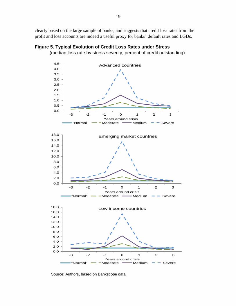
19
clearly based on the large sample of banks, and suggests that credit loss rates from the
profit and loss accounts are indeed a useful proxy for banks’ default rates and LGDs.
Figure 5. Typical Evolution of Credit Loss Rates under Stress
(median loss rate by stress severity, percent of credit outstanding)
Source: Authors, based on Bankscope data.
0.0
0.5
1.0
1.5
2.0
2.5
3.0
3.5
4.0
4.5
-3 -2 -1 0 1 2 3
Years around crisis
Advanced countries
"Normal" Moderate Medium Severe
0.0
2.0
4.0
6.0
8.0
10.0
12.0
14.0
16.0
18.0
-3 -2 -1 0 1 2 3
Years around crisis
Emerging market countries
"Normal" Moderate Medium Severe
0.0
2.0
4.0
6.0
8.0
10.0
12.0
14.0
16.0
18.0
-3 -2 -1 0 1 2 3
Years around crisis
Low income countries
"Normal" Moderate Medium Severe

20
Loss given default (LGD)
There is empirical evidence that LGDs too fluctuate with the business cycle (Figure 6; the
circled stress years are the same in Figures 2). Descriptive evidence for workout LGDs
(i.e., LGDs for bank loans) from Moody’s (2013) is used to determine changes of LGDs
under stress for ACs. The time series by Moody’s for loans, which relate to industry
averages rather than bank-by-bank results, spans the period from 1990 to 2012.25, 26
Figure 6. Evolution of LGDs through the Cycle
(Percent of the face value of affected credits)
Source: LGDs: Araten et al. (2004); Moody’s (2013); Real GDP Growth: Federal Reserve Bank
(2013).
25
A longer series for bonds is available.
26 The study by Araten et al. (2004) is based on a sample of more than 3,700 defaulted loans
(predominantly U.S. exposure) and spans the period from 1982 to 1999, covering the period of the savings
and loan crisis. Results are broadly similar to those presented here.
-4
-2
0
2
4
6
8
0
10
20
30
40
50
60
70
80
90
1982 1985 1988 1991 1994 1997 2000 2003 2006 2009 2012
Real G
DP
gro
wth
(y-o
-y)
LG
D
Real GDP Growth (US) (RHS) Araten et al (2004) (LHS)
Moody's (2013), Loans (LHS) Moody's (2013), Bonds (LHS)
21
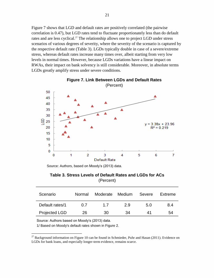
Figure 7 shows that LGD and default rates are positively correlated (the pairwise
correlation is 0.47), but LGD rates tend to fluctuate proportionately less than do default
rates and are less cyclical.27 The relationship allows one to project LGD under stress
scenarios of various degrees of severity, where the severity of the scenario is captured by
the respective default rate (Table 3). LGDs typically double in case of a severe/extreme
stress, whereas default rates increase many times over, albeit starting from very low
levels in normal times. However, because LGDs variations have a linear impact on
RWAs, their impact on bank solvency is still considerable. Moreover, in absolute terms
LGDs greatly amplify stress under severe conditions.
Figure 7. Link Between LGDs and Default Rates
(Percent)
Source: Authors, based on Moody’s (2013) data.
Table 3. Stress Levels of Default Rates and LGDs for ACs
(Percent)
27
Background information on Figure 10 can be found in Schmieder, Puhr and Hasan (2011). Evidence on
LGDs for bank loans, and especially longer-term evidence, remains scarce.
Scenario Normal Moderate Medium Severe Extreme
Default rates/1 0.7 1.7 2.9 5.0 8.4
Projected LGD 26 30 34 41 54
Source: Authors based on Moody’s (2013) data.
1/ Based on Moody's default rates shown in Figure 2.
22
LGDs for EMs and LICs are not covered due to lack of data. The historical average LGD
rates for EMs and LICs are about 59 percent and 62 percent, respectively. These LGDs
have been derived from the World Bank (Doing Business) based on Djankov et al. (2007)
and are assumed to correspond to long-term average LGDs.28 A practical approach for
stress testing purposes would be to use the long-term average level in a specific country
and, for a stress scenarios of given intensity, add the same absolute increase as seen in
ACs.
Credit losses (should) account for fluctuations in both PDs and LGDs (Box 1). One may
therefore wish to compare the default rates in Table 3 with the loss rates in Table 2 for
the ACs by dividing the loss rate by the respective LGD for the stress level. The median
long-term default rate observed in Moody’s data (0.7 percent) translates into a loss rate of
about 0.29 percent (using the LGD for the US, as determined by Schmieder and
Schmieder (2011), of 0.42). This estimated loss rate is comparable to the 0.24 percent
median loss rate for the U.S. banks in the Bankscope data (for the period covered,
i.e., 1996–2011) 29 More generally, if one divides the credit loss rates in Table 3 by the
LGDs in Table 4, the implied default rates are 1.3 percent (normal), 2.7 percent
(moderate stress), 3.3 percent (medium), 5.7 percent (severe) and 8 percent (extreme). On
the lower end, the implied default rates are higher than the actual default rates, unless one
replaces the projected LGDs by some average LGD for advanced countries (35 percent).
Overall, this result suggests that credit loss rates from the profit and loss accounts,
divided by LGD rates, provide reasonable approximations to PDs, at least for ACs. The
same applies to the implied default rates for EMs and LICs using an LGD of 60 percent.
Pre-impairment income
The next question is how pre-impairment income evolves when stress occurs, i.e.,
conditional on credit losses.30 The key components of pre-impairment operational income
28
We assume that the LGDs reported by the World Bank survey (covering 181 countries; see
http://www.doingbusiness.org) are a proxy for LGDs for corporate exposure. To account for lower LGDs
on mortgages, we assume retail LGDs of 25 percent for OECD countries, 45 percent for emerging market
countries and 50 percent for LICs. We also assume that 40 percent of total credit is retail and apply
corporate LGD rates for the remaining credit. For advanced countries, a floor of 30 percent is assumed for
corporate credit, accounting for findings in Schmieder and Schmieder (2011). The latter study investigated
recovery rates conditional on legislation, and found drivers relating, for example, to legal procedures that
account for the wide range of recovery rates.
29 If one divides the credit losses rates observed for advanced countries in Table 2 by the LGD for the
United States (0.42), the implied default becomes 0.7 percent (normal times, the global median), and
1.9 percent, 2.6 percent and 5.7 percent for moderate, medium and severe stress. This compares to
equivalent default rates (Table 4) based on long-term data from Moody’s of 0.7 percent (normal),
1.9 percent (moderate), 2.9 percent (medium) and 5 percent (severe).
30 We generally refer to net pre-impairment income, i.e., adjusted for operational expenses but not loan
losses, unless stated otherwise.
23
are (a) net interest income, which tends to be relatively stable insofar as interest rates
changes are passed on to loans and deposits when they mature; (b) net fee and
commission income; c) trading income; d) other operating income; and (e) operating
expenses. The remainder is other non-operating income, which is normally neglected
because it represents one-off items that do not affect the sustainability of a bank’s
business model. In order to normalize the measure of income despite large cross-country
differences in banks’ leverage, we focus on the ROC rather than return on assets.
Using bank-by-bank data in the Bankscope database, median net pre-impairment ROC is
found to be highest in LICs (25.0 percent), followed by EMs (18.9 percent) and then ACs
(11.9 percent), in line with expectations and accounting for the rank-order in terms of the
risk of doing business as captured by the volatility of loan losses.
Pre-impairment income conditional on credit loss rates is found to be affected in stress
scenarios, but on average to remain positive and thus a buffer against credit losses
(Figure 8 and Appendix Table 4). The behavior of income with respect to the crisis
trough tends to be less symmetric than that of credit loss rates; income often remains low
for some years after the trough (for AC banks) or drops significantly at the time of the
trough (for EM banks).31
31
The outcomes for LICs are shown in Appendix Table 4, but evidence is very limited.

24
Figure 8. Typical Evolution of Pre-impairment Income Under Stress
(Median pre-impairment ROC by stress severity; percent)
Source: Authors, based on Bankscope data.
However, there is substantial variation to this finding across banks. If one looks at the AC
banks that are more adversely affected, i.e., the worst performing 25th
and
10th
percentiles, income becomes negative for at least a quarter of banks under severe
stress (Figure 9); 10 percent of bank encounter ROCs below –20 percent at the time of
the trough under severe stress. A similar pattern can be detected for EM banks, but the
limited quantity of available data precludes firm calibration.
7.0
9.0
11.0
13.0
15.0
-3 -2 -1 0 1 2
Years around crisis
Advanced countries
"Normal" Moderate Medium Severe
10.0
13.0
16.0
19.0
22.0
25.0
28.0
-3 -2 -1 0 1 2
Years around crisis
Emerging market countries
"Normal" Moderate Medium Severe

25
Figure 9. Evolution of Pre-impairment Income for Worst Performing Banks
under Stress
(Pre-impairment ROC, percent)
Source: Authors, based on Bankscope data.
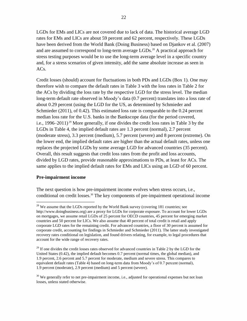
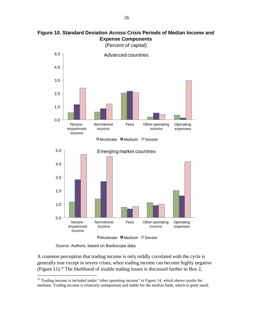
Certain earning sources seem especially vulnerable to stress conditions, as illustrated in
Figure 10 (with detailed data in Table 5A), which shows the standard deviations across
crisis periods of the median ratio to capital of various income and expense account
components. For AC banks, net commission and fee income is consistently relatively
volatile. The median AC bank’s operating expenses become very volatile in a severe
crisis, perhaps because a severe crisis will force a bank to bear restructuring costs, and
because capital is reduced. For the median EC bank, the change of net income under
stress is largely driven by net interest income due to foregone interest on credit losses
and, possibly, interest rate behavior during crises.32 EC banks manage to reduce operating
expenses at times of stress, unlike AC banks.
32
Plausibly, many EM banking crises are associated with balance of payments crises, which may lead to
higher short-term interest rates, whereas central banks in ACs react to financial sector pressure by reducing
short-term rates and can afford to ignore balance of payments effects.
-4
-2
0
2
4
6
8
10
12
14
-3 -2 -1 0 1 2 3
Years around crisis
Advanced countries-lowest 25th percentile
"Normal" Moderate Medium Severe
-25
-20
-15
-10
-5
0
5
10
15
-3 -2 -1 0 1 2 3
Years around crisis
Advanced countries-lowest 10th percentile
"Normal" Moderate Medium Severe
0
5
10
15
20
25
-3 -2 -1 0 1 2 3
Years around crisis
Emerging market countries-lowest 25th percentile
"Normal" Moderate Medium Severe
-10
-5
0
5
10
15
20
25
-3 -2 -1 0 1 2 3
Years around crisis
Emerging market countries-lowest 10th percentile
"Normal" Moderate Medium Severe
26
Figure 10. Standard Deviation Across Crisis Periods of Median Income and
Expense Components
(Percent of capital)
Source: Authors, based on Bankscope data.
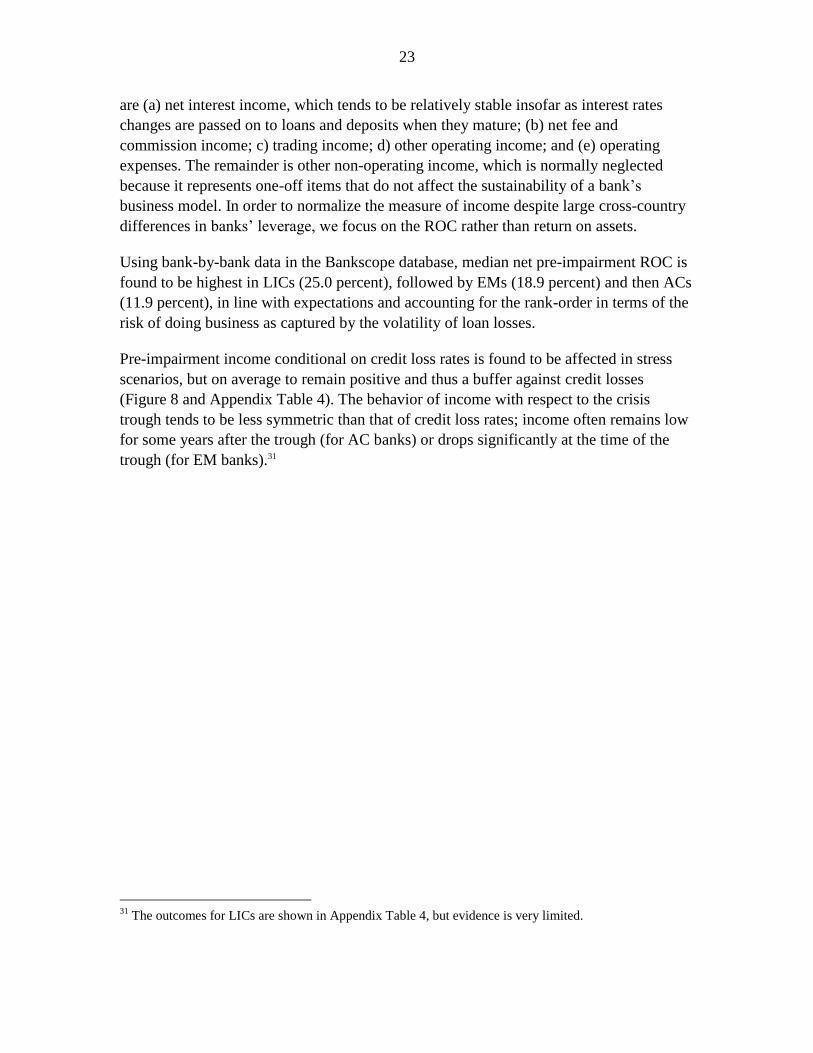
A common perception that trading income is only mildly correlated with the cycle is
generally true except in severe crises, when trading income can become highly negative
(Figure 11).33 The likelihood of sizable trading losses is discussed further in Box 2,
33
Trading income is included under “other operating income” in Figure 14, which shows results for
medians. Trading income is relatively unimportant and stable for the median bank, which is quite small.
0.0
1.0
2.0
3.0
4.0
5.0
Net pre-impairment
income
Net interest income
Fees Other operating income
Operating expenses
Advanced countries
Moderate Medium Severe
0.0
1.0
2.0
3.0
4.0
5.0
Net pre-impairment
income
Net interest income
Fees Other operating income
Operating expenses
Emerging market countries
Moderate Medium Severe
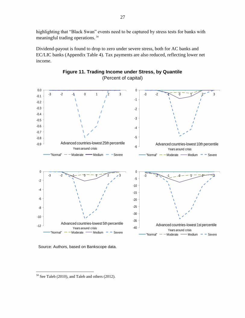
27
highlighting that “Black Swan” events need to be captured by stress tests for banks with
meaningful trading operations. 34
Dividend-payout is found to drop to zero under severe stress, both for AC banks and
EC/LIC banks (Appendix Table 4). Tax payments are also reduced, reflecting lower net
income.
Figure 11. Trading Income under Stress, by Quantile
(Percent of capital)
Source: Authors, based on Bankscope data.
34
See Taleb (2010), and Taleb and others (2012).
-0.9
-0.8
-0.7
-0.6
-0.5
-0.4
-0.3
-0.2
-0.1
0.0
-3 -2 -1 0 1 2 3
Years around crisis
Advanced countries-lowest 25th percentile
"Normal" Moderate Medium Severe
-6
-5
-4
-3
-2
-1
0
-3 -2 -1 0 1 2 3
Years around crisis
Advanced countries-lowest 10th percentile
"Normal" Moderate Medium Severe
-12
-10
-8
-6
-4
-2
0
-3 -2 -1 0 1 2 3
Years around crisis
Advanced countries-lowest 5th percentile
"Normal" Moderate Medium Severe
-40
-35
-30
-25
-20
-15
-10
-5
0
-3 -2 -1 0 1 2 3
Years around crisis
Advanced countries-lowest 1st percentile
"Normal" Moderate Medium Severe
28
Box 2. How Likely is it that Large Trading Losses Coincide with Large Credit Losses?
In many stress testing exercises in the past, no explicit link could be established between credit losses and
trading income. And there is a good reason for that, as shown in Figure 13 (upper left hand panel): for a
median bank with some trading operations, trading income is, on average, slightly positive under most
stress conditions. However, this is not necessarily the case if one moves further into the “tail,” and in
particular if one focuses on the experience of banks with sizable trading books under severe conditions.
Looking at the severe scenarios as defined by credit risk losses, a bank at the worst performing decile (in
terms of the ratio of trading income losses to capital) could lose about 5 percent of capital. The worst
performing 1 percent of banks might lose a third of capital—which would likely be more than a bank
could suffer and still survive combined with other losses and reduction of income banks would likely face
under such conditions. The severe scenario may occur with low probability, but the impact could be large,
especially because trading activity is concentrated in larger banks: the worst performing 1 percent of banks
could hold a substantial share of aggregate assets. The non-linearity and concentration of trading losses
was apparent during the recent global crisis, when a few large European banks lost within one year more
than one third of their capital due to trading losses alone, while many smaller banks had insignificant
trading losses.
Trading income is likely to follow close to a random walk pattern, with little serial correlation, so a series
of very bad years are unlikely to occur, but the simulations outlined above suggest that one bad year of
trading could enough to bring down a large bank.
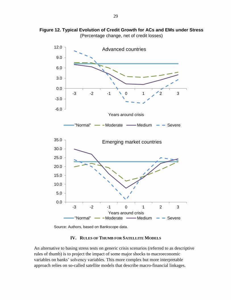
Credit growth
Banking crises affect not only the quality of a given stock of loans, but also asset and
loan growth rates; nominal credit growth of banks’ customer loans net of credit losses
tends to slow sharply, even if it does not become negative (Figure 12 and Appendix
Table 4). 35 Conditional on stress (as measured by credit losses), deleveraging occurs only
in case of severe crises in ACs, while medium intensity crises tend to end in three years
of (close to) zero year-on-year credit growth for ACs. Credit growth remains fairly
sizable for EM banks under stress, except for severe stress, when credit growth becomes
zero. Again, the pattern for the LIC banks is less clear-cut, owing to limited data. Asset
growth behaves very similarly to credit growth. Thus, both the risk-weighted capital
ratios and the unweighted leverage ratio may be affected by this effect in the
denominator.
35
This study, including in Figure 12, investigates nominal credit growth rates, and is therefore consistent
with the other factors affecting solvency, which too are measured in nominal terms.
29
Figure 12. Typical Evolution of Credit Growth for ACs and EMs under Stress
(Percentage change, net of credit losses)
Source: Authors, based on Bankscope data.
IV. RULES OF THUMB FOR SATELLITE MODELS
An alternative to basing stress tests on generic crisis scenarios (referred to as descriptive
rules of thumb) is to project the impact of some major shocks to macroeconomic
variables on banks’ solvency variables. This more complex but more interpretable
approach relies on so-called satellite models that describe macro-financial linkages.
-6.0
-3.0
0.0
3.0
6.0
9.0
12.0
-3 -2 -1 0 1 2 3
Years around crisis
Advanced countries
"Normal" Moderate Medium Severe
0.0
5.0
10.0
15.0
20.0
25.0
30.0
35.0
-3 -2 -1 0 1 2 3
Years around crisis
Emerging market countries
"Normal" Moderate Medium Severe
30
Various types of satellite models have been used in the literature to establish such
models, including time series analysis, linear and non-linear regression models (such
OLS regression, logistic regression, panel analysis) and structural models (see Foglia,
2008, and Drehmann, 2009, for example).
For the purpose of this paper, the attention focuses on fairly simple relationships, albeit
with allowance for nonlinear responses that depend on the severity and duration of strain
as measured by a shock to real GDP growth. More complex relationships might be
estimated where a stress tester has available a rich dataset, covering periods (but without
structural breaks) with a variety of shocks for a variety of banks. Yet even in such
circumstances, transparent, understandable rules of thumb may be useful in checking the
robustness of results.
It should be noted that satellite models are best suited to capturing the effects of
exogenous macroeconomic shocks, rather than shocks that originate within the financial
system, for example due to asset bubbles or large-scale malfeasance (Alfaro and
Drehmann, 2009).36 In the latter situation, the macroeconomic deterioration tends to be a
consequence of, and to follow the financial sector disturbance. Hence, the time series
properties of the satellite models should be sensitive to the origins of the disturbance.
A. Explanatory Variables and Estimation Approach
The most important single determinant of bank solvency is the overall conjunctural
conditions prevailing in the economy, which will affect all solvency factors (credit losses,
income, credit growth, and so forth). Strong economic activity should generally allow
firms to generate the revenue to repay loans, households to earn steady income to meet
debt service obligations, and collateral to retain its value. Weak economic activity will
have corresponding negative effects on a bank’s clients and thus on the bank itself.
Real GDP is normally the most relevant and most readily available measure of aggregate
activity. Policy-makers and others make frequent real GDP forecasts, and its relationship
to other macroeconomic variables is well-studied. Hence, its behavior can be readily
interpreted, and it can usually be forecast in both baseline and stress scenarios.37 The
design of scenarios is one of the key challenges for stress tests, and running a number of
potential scenarios allows studying sensitivities (Taleb et al, 2012)—a key advantage of
using rules of thumb is that they facilitate working through numerous scenarios. In what
36
Malfeasance seems to have been a major contributing factor in recent banking crises in the Dominican
Republic and Afghanistan, for example.
37 In some countries, statistics on real GDP are subject to long lags or measurement error. An index of
industrial production is often an alternative available with shorter lags and at higher frequency, but real
GDP is still normally the preferable explanatory variable because it captures a wider measure of activity.
31
follows, we will establish rules of thumb relating variables related to bank solvency to
GDP growth.
Economic intuition and evidence presented above suggests that, if economic conditions
are broadly stable and as anticipated, then only a (very) small proportion of loans will go
bad (Figure 2, Table 2). However, non-performance may increase rapidly if conditions
are unexpectedly adverse, which often happens only after a long period of benign times,
and makes such shocks all the more challenging; it is these negative “surprises” that
cause borrowers to be unable to repay and collateral to be reduced in value. Yet, as
displayed above, what counts as an exceptionally large shock in, say, the United States or
a Western European country, may be well within recent historical experience for many
EMs. Moreover, economic intuition and some empirical evidence suggest that prolonged
periods of low or negative growth will have a more pronounced effect on bank
profitability than a brief recession followed by recession
With this in mind, we computed the average (i) changes in real GDP growth at time t =
0
(the year with the lowest real GDP growth) relative to year t–4; and (ii) the cumulative
deviation of real GDP growth rates from trend from t–4 to t =
0, using World Economic
Outlook (WEO) data for both ACs and ECs.38 The cumulative deviation from trend is
likely to be more telling (given that it contains information on the duration of the shock),
but depends on an estimate of trend growth, which in some cases (e.g., following an
unsustainable burst of growth) may be difficult to obtain. A practical approach to
determine trend growth is to use the average GDP growth observed in the past over at
least one complete cycle (say, the last 10 years) or baseline forecasts (e.g., data from the
WEO). For this study, the average real GDP growth rate for 1980 to 2011 has been used
as a benchmark.
These GDP growth shocks (for the respective country type—AC or EC) are compared to
the behavior of the main variables related to bank solvency. The comparison is carried
out by various means: simple ratios and correlations are calculated, as are regressions.
The main estimates are based on bank-level and country-level evidence. Given that the
sample of bank-level data is dominated by observations from a few countries (notably the
United States), which results in limited variation for the GDP trajectories, country-level
data was used to come up with the rules. 39 However, because then the evidence is limited
to some 20 observations per country type and stress level, some parameters had to be
38
Note that the peak of the macroeconomic crisis (t =
0) is defined by the low point of GDP growth. It will
be investigated whether the macroeconomic crisis peak coincides with the banking crisis peak, as defined
previously as the year with the highest rate of credit losses.
39 The computation included only observations with a drop of GDP growth or negative cumulative
deviation, respectively, i.e., crises observations.

32
smoothed, with a view to ensure consistency across estimates: the level of the
macroeconomic shock (in terms of GDP growth) multiplied by the sensitivity of the
solvency parameters (computed based on bank- and country-level data) added to the pre-
shock level should result in broadly the same stress levels as observed under the
descriptive rules discussed above.40 While the unadjusted results achieved such
consistency in qualitative terms, the median rules were adjusted slightly to align with the
respective descriptive rules of thumb.
It must be recognized that a given macroeconomic shock will have diverse effects across
banks (and countries): some will survive quite well, and others may be devastated. Some
banks may suffer large losses in calm periods. From a stability perspective, policy-
makers are likely to be as concerned about the “tail” of weak banks as they are about the
mean or median bank; a systemic and macroeconomic problem can be created by severe
losses in just one quarter or even one tenth of the banking system. Hence, the emphasis
here is not on the median bank, but on the distribution of results across banks and in
particular the weaker banks. It turned out that the tail sensitivities, taken from the
computed country-level GDP sensitivities, deliver solvency parameters that align well
with the descriptive data for the corresponding confidence level, and represent worst case
crisis elasticities.41
Possible time lags need to be considered in making these comparisons. For both credit
loss rates and credit growth, their trajectories are found to be fairly symmetric with
respect to the crisis (see above), and the highest credit losses and lowest credit growth
levels tend to concur with the year of the lowest real GDP growth. Hence, the results
reported refer to coincident effects. Because pre-impairment income is less symmetric
with respect to financial stress (conditional on credit losses; Figures 9 and 11), changes of
real GDP growth rates are compared with the subsequent changes of pre-impairment
income, with a view to err on the conservative side. For ACs, the change in income is
computed as the minimum income level observed between t= 0 and t=
3, minus the initial
income level at t= –4. For ECs, income tends to remain high until stress materializes;
40
The implied sensitivity, i.e., the sensitivity based on inferring the sensitivities from the “average” size of
the macroeconomic shock and the level of the solvency parameters computed based on the descriptive
rules, is slightly higher than the one computed as the ratio of change of solvency parameter and change of
GDP growth rates. This discrepancy arises because macroeconomic stress and financial stress are not
always temporally aligned, and because idiosyncratic factors at the bank level are also at play. The
proposed rules using the implied sensitivities makes the rules more conservative, in line with the purpose
for stress testing, and consistent with the descriptive rules.
41 The 5
th-tile of the elasticities in Table 4 represents a tail level sensitivity, but does not correspond to the
single most extreme cases observed in the past. Credit losses in Iceland, an AC country, peaked at well
above the 4.3 loss rate, the “extreme” AC level in Table 3. Using the first percentile for the credit loss
sensitivity for the “drop in GDP” rule in Table 4, for example, would yield a sensitivity of -2.5,
corresponding to an increase on the credit loss rate to more than 30 percent, as observed for Iceland.

33
hence, the average income in t= –3 to t=
0 is compared with the minimum income level
after t= 0 (in Appendix Table 4).
While the data available for LICs were sufficient to come up with some meaningful
descriptions of the typical behavior of aggregates in financial crises, comparatively little
data were available to investigate macro-financial linkages. Hence, macro-financial
satellite rules of thumb are not reported for LICs.
B. Rules of Thumb for Satellite Models
Table 4 summarizes the estimated real GDP growth sensitivities of credit losses, pre-
impairment income and credit growth, distinguishing, as before, among moderate,
medium and severe stress (as measured by the real GDP growth paths), and between ACs
and EMs.
The table provides two different sets of rules, based either on cumulative changes in
growth rates or on the change in the annual growth rates from pre-crisis to crisis trough. 42
Each approach might be useful for stress tests in certain circumstances. For example, one
first establishes a scenario in terms of cumulative deviation of real GDP growth rates
from trend during the years up to the trough of the stress period (such as 5.9 percentage
points for the moderate stress in an AC), which deviation is multiplied by the
corresponding sensitivity parameter—in this case leading to an increase in median bank
credit losses of –5.9×–0.1 =
0.59 percentage points in the worst year. Projections based on
changes in annual growth rates work similarly: for an AC, for example, one could
simulate the impact of a drop of real GDP growth rate from before the recession (perhaps
2.4 percent, the average real GDP growth rate in ACs during 1980–2011), to 0.0 percent
(the moderate scenario for ACs), to –1.9 percent (medium stress), or to –5.0 percent
(severe stress) at the trough. The median AC bank’s credit losses would increase by –
2.4×–0.2 =
0.48 percentage points, –4.3×–0.2
=
0.86 percentage points, and –7.4×–0.4
=
2.96 percentage points, respectively.
Projections along the path from pre-crisis to peak crisis can be calculated. For the rule
based on changes of annual growth rates from pre-crisis levels and assuming moderate
stress, for example, one would establish the level of solvency parameters as follows: for
t = –3, the assumption of an initial drop of GDP by 0.3 percent, say, would yield loss
rates of 0.36 (0.3 percent plus –0.3×–0.2). For the next year (t = –2), the same sensitivity
(0.2) would be multiplied with the change in the growth rate and added to previous year’s
level, and so on.
42 The cumulative deviations of GDP growth are about twice the level of the change in annual real GDP
growth rates for the ACs, and about three times in the case of the ECs, suggesting that macroeconomic
crises in the ECs are longer and deeper.
34
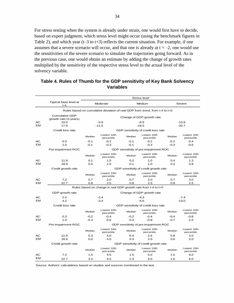
For stress testing when the system is already under strain, one would first have to decide,
based on expert judgment, which stress level might occur (using the benchmark figures in
Table 2), and which year (t–3 to t+3) reflects the current situation. For example, if one
assumes that a severe scenario will occur, and that one is already at t = –2, one would use
the sensitivities of the severe scenario to simulate the trajectories going forward. As in
the previous case, one would obtain an estimate by adding the change of growth rates
multiplied by the sensitivity of the respective stress level to the actual level of the
solvency variable.
Table 4. Rules of Thumb for the GDP sensitivity of Key Bank Solvency
Variables
Stress level
Typical base level at
t-4Moderate Medium Severe Moderate
Rules based on cumulative deviation of real GDP from trend, from t-4 to t=0
Cumulative GDP
growth rate (4 years)Change of GDP growth rate
AC 10.0
EM 17.9
Credit loss rate GDP sensitivity of credit loss rate
MedianLowest 10th
percentileMedian
Lowest 10th
percentileMedian
Lowest 10th
percentile
AC 0.3 -0.1 -0.2 -0.1 -0.2 -0.2 -0.4
EM 1.0 -0.1 -0.3 -0.1 -0.3 -0.3 -0.6
Pre-impairment ROC GDP sensitivity of pre-impairment ROC
MedianLowest 10th
percentileMedian
Lowest 10th
percentileMedian
Lowest 10th
percentile
AC 11.9 0.1 1.5 0.2 1.0 0.4 1.3
EM 18.9 0.0 1.5 0.1 1.0 0.2 0.8
Credit growth rate GDP sensitivity of credit growth rate
MedianLowest 10th
percentileMedian
Lowest 10th
percentileMedian
Lowest 10th
percentile
AC 7.2 0.7 2.0 0.7 2.0 0.7 3.0
EM 22.7 0.8 2.5 0.8 2.5 0.8 2.5
Rules based on change in real GDP growth rate from t-4 to t=0
GDP growth rate Change of GDP growth rate
AC 2.4
EM 4.2
Credit loss rate GDP sensitivity of credit loss rate
MedianLowest 10th
percentileMedian
Lowest 10th
percentileMedian
Lowest 10th
percentile
AC 0.3 -0.2 -0.4 -0.2 -0.4 -0.4 -0.8
EM 1.0 -0.4 -0.6 -0.4 -0.8 -0.7 -1.5
Pre-impairment ROC GDP sensitivity of pre-impairment ROC
MedianLowest 10th
percentileMedian
Lowest 10th
percentileMedian
Lowest 10th
percentile
AC 11.9 0.3 4.0 0.4 2.5 0.8 2.0
EM 18.9 0.0 4.0 0.3 2.0 0.6 2.0
Credit growth rate GDP sensitivity of credit growth rate
MedianLowest 10th
percentileMedian
Lowest 10th
percentileMedian
Lowest 10th
percentile
AC 7.2 1.5 4.5 1.5 5.0 1.5 6.0
EM 22.7 3.2 4.5 2.3 5.0 1.6 6.0
Source: Authors' calculations based on studies and sources mentioned in the text.
-2.4 -4.3 -7.4
-3.4 -6.6 -13.0
-5.9 -8.5 -13.9
-11.5 -19.5 -32.7
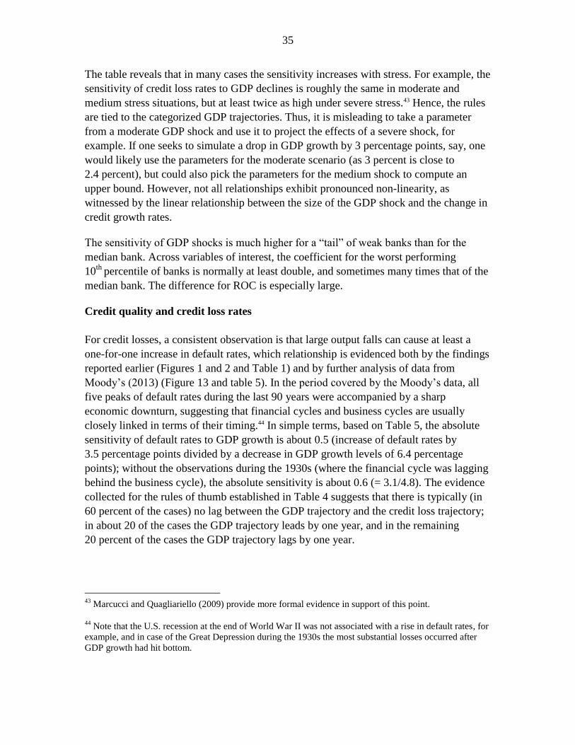
35
The table reveals that in many cases the sensitivity increases with stress. For example, the
sensitivity of credit loss rates to GDP declines is roughly the same in moderate and
medium stress situations, but at least twice as high under severe stress.43 Hence, the rules
are tied to the categorized GDP trajectories. Thus, it is misleading to take a parameter
from a moderate GDP shock and use it to project the effects of a severe shock, for
example. If one seeks to simulate a drop in GDP growth by 3 percentage points, say, one
would likely use the parameters for the moderate scenario (as 3 percent is close to
2.4 percent), but could also pick the parameters for the medium shock to compute an
upper bound. However, not all relationships exhibit pronounced non-linearity, as
witnessed by the linear relationship between the size of the GDP shock and the change in
credit growth rates.
The sensitivity of GDP shocks is much higher for a “tail” of weak banks than for the
median bank. Across variables of interest, the coefficient for the worst performing
10th
percentile of banks is normally at least double, and sometimes many times that of the
median bank. The difference for ROC is especially large.
Credit quality and credit loss rates
For credit losses, a consistent observation is that large output falls can cause at least a
one-for-one increase in default rates, which relationship is evidenced both by the findings
reported earlier (Figures 1 and 2 and Table 1) and by further analysis of data from
Moody’s (2013) (Figure 13 and table 5). In the period covered by the Moody’s data, all
five peaks of default rates during the last 90 years were accompanied by a sharp
economic downturn, suggesting that financial cycles and business cycles are usually
closely linked in terms of their timing.44 In simple terms, based on Table 5, the absolute
sensitivity of default rates to GDP growth is about 0.5 (increase of default rates by
3.5 percentage points divided by a decrease in GDP growth levels of 6.4 percentage
points); without the observations during the 1930s (where the financial cycle was lagging
behind the business cycle), the absolute sensitivity is about 0.6 (= 3.1/4.8). The evidence
collected for the rules of thumb established in Table 4 suggests that there is typically (in
60 percent of the cases) no lag between the GDP trajectory and the credit loss trajectory;
in about 20 of the cases the GDP trajectory leads by one year, and in the remaining
20 percent of the cases the GDP trajectory lags by one year.
43
Marcucci and Quagliariello (2009) provide more formal evidence in support of this point.
44 Note that the U.S. recession at the end of World War II was not associated with a rise in default rates, for
example, and in case of the Great Depression during the 1930s the most substantial losses occurred after
GDP growth had hit bottom.
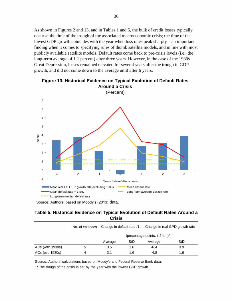
36
As shown in Figures 2 and 13, and in Tables 1 and 5, the bulk of credit losses typically
occur at the time of the trough of the associated macroeconomic crisis; the time of the
lowest GDP growth coincides with the year when loss rates peak sharply—an important
finding when it comes to specifying rules of thumb satellite models, and in line with most
publicly available satellite models. Default rates come back to pre-crisis levels (i.e., the
long-term average of 1.1 percent) after three years. However, in the case of the 1930s
Great Depression, losses remained elevated for several years after the trough in GDP
growth, and did not come down to the average until after 6 years.
Figure 13. Historical Evidence on Typical Evolution of Default Rates
Around a Crisis
(Percent)
Source: Authors, based on Moody’s (2013) data.
Table 5. Historical Evidence on Typical Evolution of Default Rates Around a
Crisis
-1
0
1
2
3
4
5
6
7
8
-3 -2 -1 0 1 2 3
Perc
ent
Years before/af ter a crisis
Mean real US GDP growth rate excluding 1930s Mean default rate
Mean default rate + 1 StD Long-term average default rate
Long-term median default rate
No. of episodes
(percentage points, t-4 to t)/
Average StD Average StD
ACs (with 1930s) 5 3.5 1.6 -6.4 3.9
ACs (w/o 1930s) 4 3.1 1.6 -4.8 1.6
1/ The trough of the crisis is set by the year with the lowest GDP growth.
Source: Authors' calculations based on Moody's and Federal Reserve Bank data.
Change in default rate /1 Change in real GPD growth rate
37
This is in line with GDP elasticities found based on the sample data from Bankscope
(Table 4), where one can clearly observe the non-linear (convex) pattern of credit loss
rates, with the sensitivities increasing sharply as one moves from moderate to severe
stress. The table also reveals that the GDP sensitivity of loss rates in EMs is considerably
higher than that found in ACs, and becomes close to one-for-one or more under severe
conditions.45
For default rates, Moody’s (2013) data are used to compute GDP sensitivities for ACs
(Table 6), which turn out to be qualitatively similar to loss rates computed based on bank-
by-bank data discussed above. Again, the parameters in the table are meant to be used
together with the GDP trajectories for the ACs from Table 4. For projections based on the
cumulative deviation of GDP growth from trend, the parameters should be divided by
two.
Table 6. Rules of Thumb for the GDP Growth Sensitivity of Credit Risk
Parameters
Moderate Medium Severe
Default rates
-0.4 -0.6 -0.8
LGDs
-1.5 -2.5 -4.0
Asset correlations (corporates)
-2.7
Source: Authors, based on studies and sources mentioned in the text.
LGD
The correlation between LGDs for loans from Moody’s (2013) with GDP real growth
rates is -0.44, indicating that LGDs are lower during periods of higher output (see also
Figure 6). The evidence on hand, however, suggests that the sensitivity of LGD rates to a
real GDP slowdown is usually moderate in ACs, given that LGD even in normal times is
typically in the 30 to 60 percent range; the sensitivity (in relative terms) is lower than that
45
The coefficients for moderate stress are in line with research Cerutti et al. (2010), for example, who used
a linear panel model for emerging Europe. If one uses non-linear specifications and/or does not control for
effects other than GDP growth (i.e., measures the impact of a macroeconomic shock by means of changes
in GDP growth alone), the coefficients tend to be higher, which indicates that the established coefficients
are robust.

38
of PDs (Table 6). For ECs, there is not enough evidence to come up with separate
parameters, but the parameters for ACs could be used as a starting point.
However, these rules of thumb for LGD (which are especially low for moderate and
medium stress scenarios) , are unlikely to apply when the source of the shock is related to
the bursting of an asset price bubble: the end of an asset price bubble and in particular a
debt-financed real estate bubble entails that much of the collateral backing the lending
has suffered a drastic reduction in value, and the market for it has become much less
liquid. Hence, LGD rates should be expected to be exceptionally high in such situations.
A practical approach could be to use the coefficient from the severe scenario even when
the macroeconomic shock is moderate or medium.
Income
As it was done for credit losses, Table 4 compares the changes in GDP to changes in pre-
impairment income. The median GDP sensitivities of income are relative modest, but the
relationship can become highly non-linear in unfavorable circumstances, in line with
Figure 10, and especially for a substantial portion of poorly-performing banks.
Retained earnings
Profits translate into capital directly through the retention of earnings. A bank that makes
losses would normally be expected to “retain” all these losses in the form of a reduction
in its capital ratio. A bank that makes profits but has low capitalization would be
expected to retain all or almost all profits.46 But a bank that is both profitable and well-
capitalized would normally pay out a noteworthy portion of its net income (or extend its
balance sheet, when perhaps macro-prudential policy is warranted; see IMF, 2011b),
without substantially running-down its capital to do so. Such behavior can easily be
incorporated into a rule of thumb.47
The expected levels of profit retention by banks under stress are shown in Appendix
Table 4. AC banks are found to pay-out about 35 percent in “normal” times and moderate
stress times, 20 percent under medium stress, and zero under severe stress. For the EM
and AC banks, the levels are similar, at around 30 (EM) and 45 (LIC) in normal times
and moderate stress, 17 (EM) and 40 (LIC) under medium stress, and 0 under severe
stress.
46
Basel III has defined minimum regulatory rates for retention of income (“capital conservation”) (BCBS,
2011, para. 131).
47 It is easy to show that, if a bank’s total assets tend to grow at a rate g and its return on equity tends to be
ρ, then its leverage ratio will remain constant if it retains a proportion (g/ρ) of its net profits.

39
Credit growth
For credit growth, the rule foresees similar GDP sensitivities for AC banks across shock
levels. The sensitivity in ECs tends to decrease with stress intensity, which result may be
influenced by the comparatively high credit growth rates, especially in EC countries
during the last 15 year. Going forward, the trend might change as EM financial systems
mature, which is why these rules should be used carefully.
In applying these rules of thumb, it will again be important to make allowance for the
origins of the simulated financial crisis: a crisis provoked by an external macroeconomic
shock is likely to be associated with relatively stable credit aggregates or only a more
moderate slowdown. A crisis provoked by the bursting of a credit-financed asset price
bubble or a lending boom is likely to be followed by a more contractionary path for credit
aggregates.
Asset correlations
Asset correlations are one of the solvency parameters that have been studied less
intensely, despite their important impact on capital ratios. Besides the scarcity of long-
term data, one reason for the relative neglect may be that IRB asset correlations are
determined conditional on the level of PDs, based on a cross-sectional rule that foresees
that lower PDs are associated with higher asset correlations.48 Using either IRB asset
correlations (or fixed asset correlations) may be appropriate for supervisory purposes
because the approach avoids possible double-counting of potential stress when losses
have already materialized (and affect the numerator of capital ratios), while the
denominator (RWAs) (still) foresees the potential for elevated potential losses. However,
if one takes a multi-period, stress testing view, this relationship could be misleading, as
illustrated below.
To determine the fluctuations of asset correlations under macroeconomic stress, we refer
to a study by Duellmann and others (2008) based on a sample of data on large,
predominantly Western European corporate.49 During a period of six years (1997–2003),
asset correlations fluctuated strongly, ranging from 4 percent to 16 percent, with a mean
at 10.5 percent (Appendix Figure 2).50 We find a high GDP growth sensitivity of -2.7
48
This rule reflects the empirical fact that the credit quality of larger firms exhibit higher correlation with
the cycle.
49 The study revealed median monthly figures calculated based on 24-month sliding windows for the
sample of European firms in the Moody’s KMV database.
50 This level is in line with those provided in Lopez (2004).
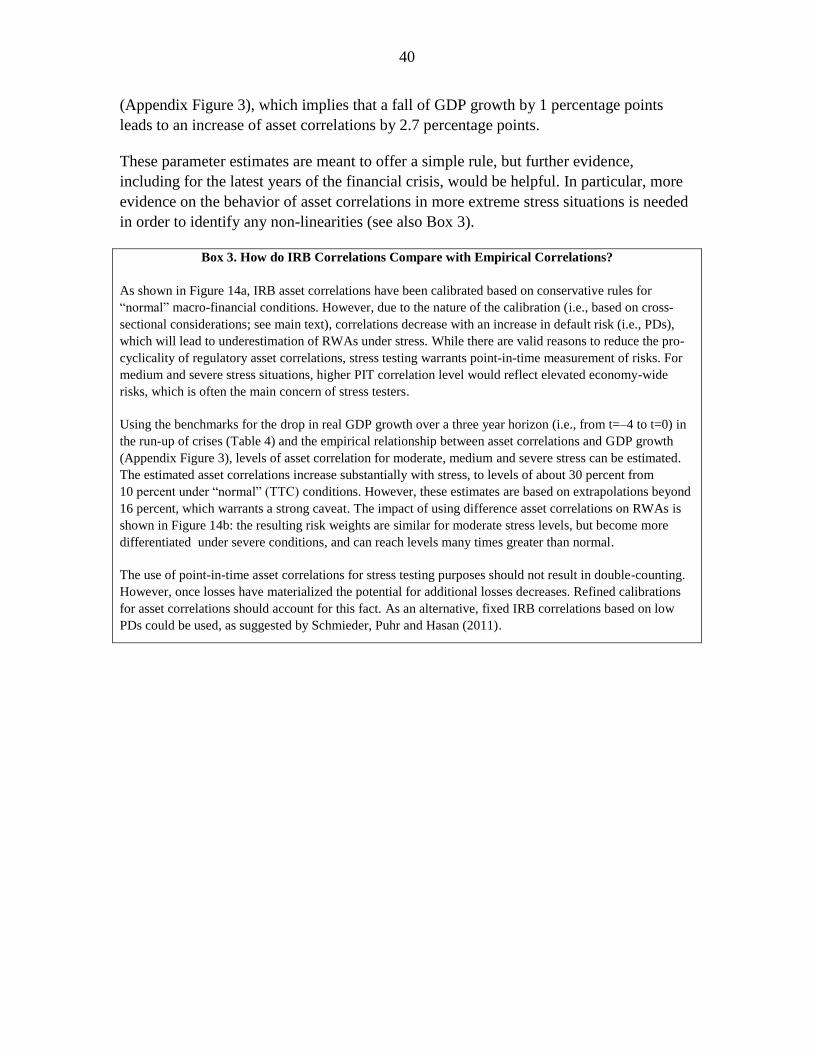
40
(Appendix Figure 3), which implies that a fall of GDP growth by 1 percentage points
leads to an increase of asset correlations by 2.7 percentage points.
These parameter estimates are meant to offer a simple rule, but further evidence,
including for the latest years of the financial crisis, would be helpful. In particular, more
evidence on the behavior of asset correlations in more extreme stress situations is needed
in order to identify any non-linearities (see also Box 3).
Box 3. How do IRB Correlations Compare with Empirical Correlations?
As shown in Figure 14a, IRB asset correlations have been calibrated based on conservative rules for
“normal” macro-financial conditions. However, due to the nature of the calibration (i.e., based on cross-
sectional considerations; see main text), correlations decrease with an increase in default risk (i.e., PDs),
which will lead to underestimation of RWAs under stress. While there are valid reasons to reduce the pro-
cyclicality of regulatory asset correlations, stress testing warrants point-in-time measurement of risks. For
medium and severe stress situations, higher PIT correlation level would reflect elevated economy-wide
risks, which is often the main concern of stress testers.
Using the benchmarks for the drop in real GDP growth over a three year horizon (i.e., from t=–4 to t=0) in
the run-up of crises (Table 4) and the empirical relationship between asset correlations and GDP growth
(Appendix Figure 3), levels of asset correlation for moderate, medium and severe stress can be estimated.
The estimated asset correlations increase substantially with stress, to levels of about 30 percent from
10 percent under “normal” (TTC) conditions. However, these estimates are based on extrapolations beyond
16 percent, which warrants a strong caveat. The impact of using difference asset correlations on RWAs is
shown in Figure 14b: the resulting risk weights are similar for moderate stress levels, but become more
differentiated under severe conditions, and can reach levels many times greater than normal.
The use of point-in-time asset correlations for stress testing purposes should not result in double-counting.
However, once losses have materialized the potential for additional losses decreases. Refined calibrations
for asset correlations should account for this fact. As an alternative, fixed IRB correlations based on low
PDs could be used, as suggested by Schmieder, Puhr and Hasan (2011).
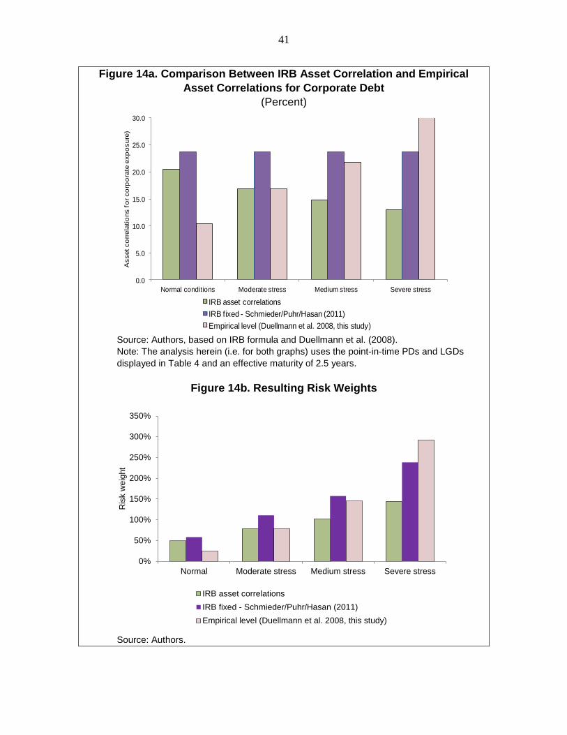
41
Figure 14a. Comparison Between IRB Asset Correlation and Empirical
Asset Correlations for Corporate Debt
(Percent)
Source: Authors, based on IRB formula and Duellmann et al. (2008).
Note: The analysis herein (i.e. for both graphs) uses the point-in-time PDs and LGDs
displayed in Table 4 and an effective maturity of 2.5 years.
Figure 14b. Resulting Risk Weights
Source: Authors.
0.0
5.0
10.0
15.0
20.0
25.0
30.0
Normal conditions Moderate stress Medium stress Severe stress
Asset co
rrela
tio
ns f
or co
rpo
rate
exp
osure
)
IRB asset correlations
IRB fixed - Schmieder/Puhr/Hasan (2011)
Empirical level (Duellmann et al. 2008, this study)
0%
50%
100%
150%
200%
250%
300%
350%
Normal Moderate stress Medium stress Severe stress
Ris
k w
eig
ht
IRB asset correlations
IRB fixed - Schmieder/Puhr/Hasan (2011)
Empirical level (Duellmann et al. 2008, this study)
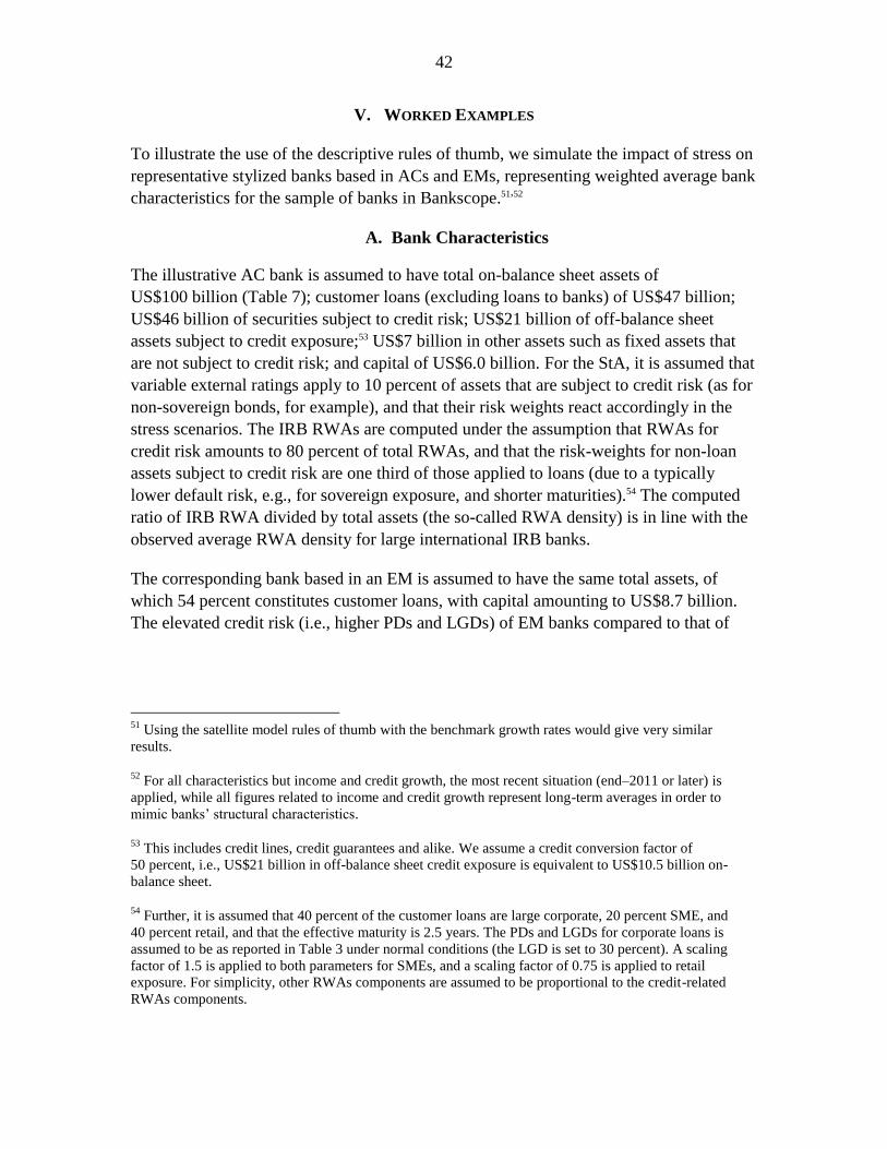
42
V. WORKED EXAMPLES
To illustrate the use of the descriptive rules of thumb, we simulate the impact of stress on
representative stylized banks based in ACs and EMs, representing weighted average bank
characteristics for the sample of banks in Bankscope.51,52
A. Bank Characteristics
The illustrative AC bank is assumed to have total on-balance sheet assets of
US$100 billion (Table 7); customer loans (excluding loans to banks) of US$47 billion;
US$46 billion of securities subject to credit risk; US$21 billion of off-balance sheet
assets subject to credit exposure;53 US$7 billion in other assets such as fixed assets that
are not subject to credit risk; and capital of US$6.0 billion. For the StA, it is assumed that
variable external ratings apply to 10 percent of assets that are subject to credit risk (as for
non-sovereign bonds, for example), and that their risk weights react accordingly in the
stress scenarios. The IRB RWAs are computed under the assumption that RWAs for
credit risk amounts to 80 percent of total RWAs, and that the risk-weights for non-loan
assets subject to credit risk are one third of those applied to loans (due to a typically
lower default risk, e.g., for sovereign exposure, and shorter maturities).54 The computed
ratio of IRB RWA divided by total assets (the so-called RWA density) is in line with the
observed average RWA density for large international IRB banks.
The corresponding bank based in an EM is assumed to have the same total assets, of
which 54 percent constitutes customer loans, with capital amounting to US$8.7 billion.
The elevated credit risk (i.e., higher PDs and LGDs) of EM banks compared to that of
51
Using the satellite model rules of thumb with the benchmark growth rates would give very similar
results.
52 For all characteristics but income and credit growth, the most recent situation (end–2011 or later) is
applied, while all figures related to income and credit growth represent long-term averages in order to
mimic banks’ structural characteristics.
53 This includes credit lines, credit guarantees and alike. We assume a credit conversion factor of
50 percent, i.e., US$21 billion in off-balance sheet credit exposure is equivalent to US$10.5 billion on-
balance sheet.
54 Further, it is assumed that 40 percent of the customer loans are large corporate, 20 percent SME, and
40 percent retail, and that the effective maturity is 2.5 years. The PDs and LGDs for corporate loans is
assumed to be as reported in Table 3 under normal conditions (the LGD is set to 30 percent). A scaling
factor of 1.5 is applied to both parameters for SMEs, and a scaling factor of 0.75 is applied to retail
exposure. For simplicity, other RWAs components are assumed to be proportional to the credit-related
RWAs components.

43
AC banks result in relatively high capital weights under IRB, and therefore a lower
capital ratio. 55, 56
Table 7. Features of Banks Used in the Worked Examples
(US$ billions)
Example bank ACs EMs
Assets 100.0 100.0
of which:
Customer loans 47.0 54.0
Other on-balance sheet assets subject to credit risk 46.0 39.0
Assets not subject to credit risk 7.0 7.0
Off-balance sheet assets subject to credit risk 21.0 24.0
Total regulatory capital 6.0 8.7
Leverage ratio (capital/(on + off-balance assets)) 5.0 7.1
StA RWAs (US$ billions) 1/ 64.3 62.0
StA capital ratio (percent) 2/ 9.3 14.0
Implied IRB RWAs (US$ billions) 3/ 40.9 107.4
Implied IRB capital ratio (percent) 2/ 14.7 8.1
Pre-impairment income (ROC, percent, long-term average) 12.0 20.0
Net income (US$ billions, long-term average) 0.4 1.1
ROC (percent, long-term average) 6.7 9.3
Source: Authors, based on Bankscope data. 1/ AC: weighted average for banks with total assets less than US$100 billion. EC: weighted average of all banks.
2/ Capital divided by respective RWAs. 3/ Estimated based on the sensitivities presented in this study, assuming that 20 percent of RWAs are accounted for by other risk types (such as market risk and operational risk).
Simulations
55
A risky asset could require more than 8 percent minimum capital, implying a risk weights over
100 percent.
56 The fact that the EC’s IRB-based capital ratio (8.1 percent) under normal conditions is well below the
EC’s StA capital ratio (14.0 percent) suggests that EC banks should not normally expect an increase of
capital ratios when they move to the IRB.
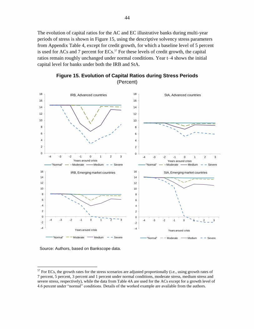
44
The evolution of capital ratios for the AC and EC illustrative banks during multi-year
periods of stress is shown in Figure 15, using the descriptive solvency stress parameters
from Appendix Table 4, except for credit growth, for which a baseline level of 5 percent
is used for ACs and 7 percent for ECs.57 For these levels of credit growth, the capital
ratios remain roughly unchanged under normal conditions. Year t–4 shows the initial
capital level for banks under both the IRB and StA.
Figure 15. Evolution of Capital Ratios during Stress Periods
(Percent)
Source: Authors, based on Bankscope data.
57
For ECs, the growth rates for the stress scenarios are adjusted proportionally (i.e., using growth rates of
7 percent, 5 percent, 3 percent and 1 percent under normal conditions, moderate stress, medium stress and
severe stress, respectively), while the data from Table 4A are used for the ACs except for a growth level of
4.6 percent under “normal” conditions. Details of the worked example are available from the authors.
0
2
4
6
8
10
12
14
16
18
-4 -3 -2 -1 0 1 2 3
Years around crisis
IRB, Advanced countries
"Normal" Moderate Medium Severe
0
2
4
6
8
10
12
14
16
18
-4 -3 -2 -1 0 1 2 3
Years around crisis
StA, Advanced countries
"Normal" Moderate Medium Severe
-4
-2
0
2
4
6
8
10
12
14
16
-4 -3 -2 -1 0 1 2 3
Years around crisis
IRB, Emerging market countries
"Normal" Moderate Medium Severe
-4
-2
0
2
4
6
8
10
12
14
16
-4 -3 -2 -1 0 1 2 3
Years around crisis
StA, Emerging market countries
"Normal" Moderate Medium Severe
45
For AC banks under the IRB, severe stress will reduce capital levels to 3 percent,
i.e., below the regulatory minimum of 8 percent, and medium level stress also reduces
capital levels substantially, to about 7 percent from an initial level of 14.7 percent.
Moderate stress can be digested by banks.
Measured bank capitalization under the StA is generally affected less by stress than that
under the IRB approach, largely due to the more substantial changes in RWAs under the
IRB, especially under severe stress (Table 8, which shows RWA as a proportion of total
assets so as to normalize for the effects of balance sheet growth). Variations in RWAs
based on PIT credit risk parameters (PD, LGD) are very sizable in the absence of
mitigation through behavioral adjustments (e.g., re-balancing of assets toward highly-
rated securities).
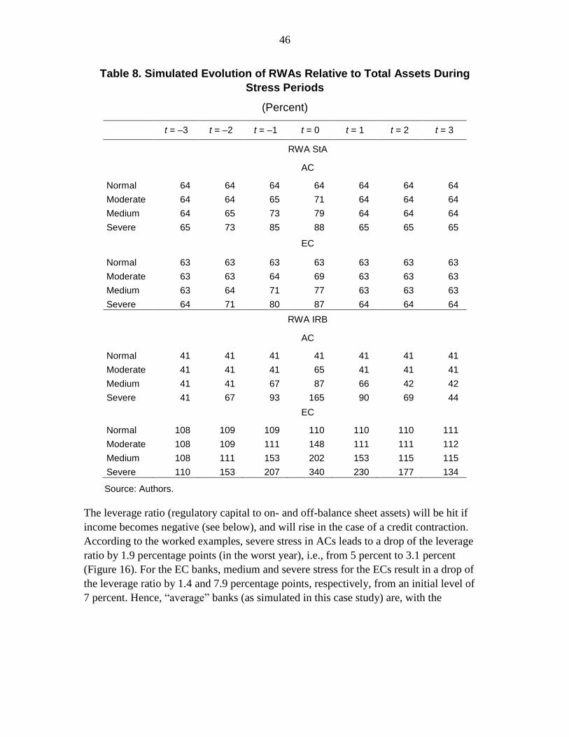
46
Table 8. Simulated Evolution of RWAs Relative to Total Assets During
Stress Periods
(Percent)
t = –3 t = –2 t = –1 t = 0 t = 1 t = 2 t = 3
RWA StA
AC
Normal 64 64 64 64 64 64 64
Moderate 64 64 65 71 64 64 64
Medium 64 65 73 79 64 64 64
Severe 65 73 85 88 65 65 65
EC
Normal 63 63 63 63 63 63 63
Moderate 63 63 64 69 63 63 63
Medium 63 64 71 77 63 63 63
Severe 64 71 80 87 64 64 64
RWA IRB
AC
Normal 41 41 41 41 41 41 41
Moderate 41 41 41 65 41 41 41
Medium 41 41 67 87 66 42 42
Severe 41 67 93 165 90 69 44
EC
Normal 108 109 109 110 110 110 111
Moderate 108 109 111 148 111 111 112
Medium 108 111 153 202 153 115 115
Severe 110 153 207 340 230 177 134
Source: Authors.
The leverage ratio (regulatory capital to on- and off-balance sheet assets) will be hit if
income becomes negative (see below), and will rise in the case of a credit contraction.
According to the worked examples, severe stress in ACs leads to a drop of the leverage
ratio by 1.9 percentage points (in the worst year), i.e., from 5 percent to 3.1 percent
(Figure 16). For the EC banks, medium and severe stress for the ECs result in a drop of
the leverage ratio by 1.4 and 7.9 percentage points, respectively, from an initial level of
7 percent. Hence, “average” banks (as simulated in this case study) are, with the
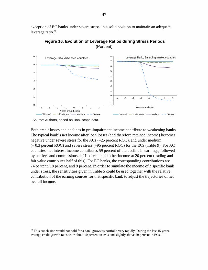
47
exception of EC banks under severe stress, in a solid position to maintain an adequate
leverage ratio.58
Figure 16. Evolution of Leverage Ratios during Stress Periods
(Percent)
Source: Authors, based on Bankscope data.
Both credit losses and declines in pre-impairment income contribute to weakening banks.
The typical bank’s net income after loan losses (and therefore retained income) becomes
negative under severe stress for the ACs (–25 percent ROC), and under medium
(– 0.3 percent ROC) and severe stress (–95 percent ROC) for the ECs (Table 9). For AC
countries, net interest income contributes 59 percent of the decline in earnings, followed
by net fees and commissions at 21 percent, and other income at 20 percent (trading and
fair value contributes half of this). For EC banks, the corresponding contributions are
74 percent, 18 percent, and 9 percent. In order to simulate the income of a specific bank
under stress, the sensitivities given in Table 5 could be used together with the relative
contribution of the earning sources for that specific bank to adjust the trajectories of net
overall income.
58
This conclusion would not hold for a bank grows its portfolio very rapidly. During the last 15 years,
average credit growth rates were about 10 percent in ACs and slightly above 20 percent in ECs.
0
1
2
3
4
5
6
-4 -3 -2 -1 0 1 2 3
Years around crisis
Leverage ratio, Advanced countries
"Normal" Moderate Medium Severe
-2
-1
0
1
2
3
4
5
6
7
8
-4 -3 -2 -1 0 1 2 3
Years around crisis
Leverage Ratio, Emerging market countries
"Normal" Moderate Medium Severe
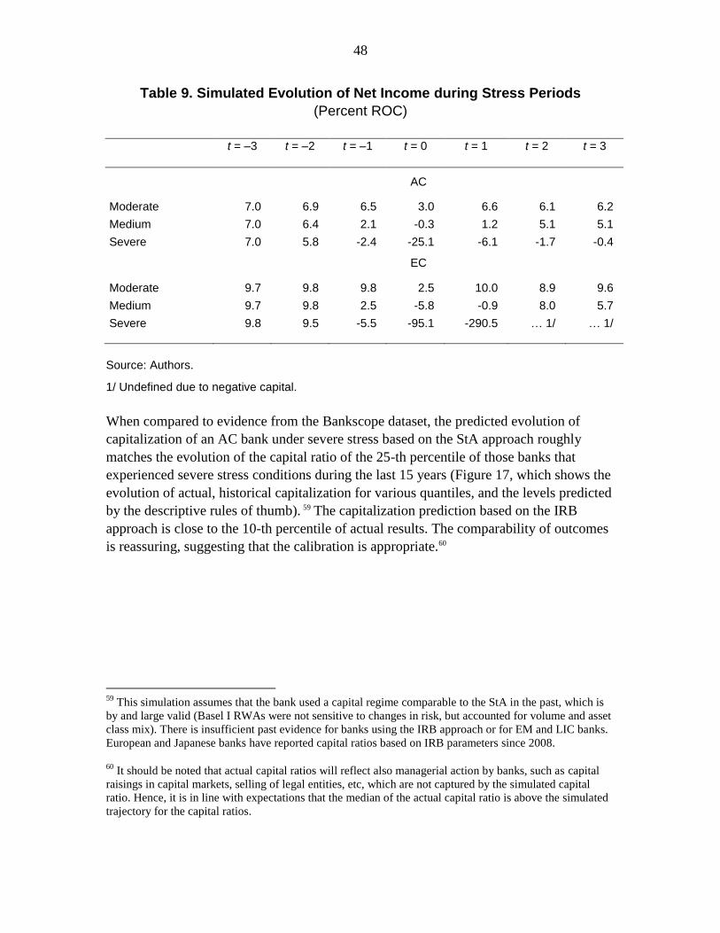
48
Table 9. Simulated Evolution of Net Income during Stress Periods
(Percent ROC)
t = –3 t = –2 t = –1 t = 0 t = 1 t = 2 t = 3
AC
Moderate 7.0 6.9 6.5 3.0 6.6 6.1 6.2
Medium 7.0 6.4 2.1 -0.3 1.2 5.1 5.1
Severe 7.0 5.8 -2.4 -25.1 -6.1 -1.7 -0.4
EC
Moderate 9.7 9.8 9.8 2.5 10.0 8.9 9.6
Medium 9.7 9.8 2.5 -5.8 -0.9 8.0 5.7
Severe 9.8 9.5 -5.5 -95.1 -290.5 … 1/ … 1/
Source: Authors.
1/ Undefined due to negative capital.
When compared to evidence from the Bankscope dataset, the predicted evolution of
capitalization of an AC bank under severe stress based on the StA approach roughly
matches the evolution of the capital ratio of the 25-th percentile of those banks that
experienced severe stress conditions during the last 15 years (Figure 17, which shows the
evolution of actual, historical capitalization for various quantiles, and the levels predicted
by the descriptive rules of thumb). 59
The capitalization prediction based on the IRB
approach is close to the 10-th percentile of actual results. The comparability of outcomes
is reassuring, suggesting that the calibration is appropriate.60
59
This simulation assumes that the bank used a capital regime comparable to the StA in the past, which is
by and large valid (Basel I RWAs were not sensitive to changes in risk, but accounted for volume and asset
class mix). There is insufficient past evidence for banks using the IRB approach or for EM and LIC banks.
European and Japanese banks have reported capital ratios based on IRB parameters since 2008.
60 It should be noted that actual capital ratios will reflect also managerial action by banks, such as capital
raisings in capital markets, selling of legal entities, etc, which are not captured by the simulated capital
ratio. Hence, it is in line with expectations that the median of the actual capital ratio is above the simulated
trajectory for the capital ratios.

49
Figure 17. Evolution of Capital Ratios: Actual vs. Predicted for an AC Bank
(Percent)
Source: Authors, based on Bankscope data (2,050 observations).
As another means of comparison, the rules for the satellite models were applied in the
context of recent stress tests run for EU and U.S. banks. Again the results were re-
assuring (Box 4).
IRB-based prediction
StA-based prediction

50
Box 4. Rules of Thumb Applied to Recent Stress Tests
The satellite model rules of thumb are applied to the scenarios used in recent stress tests run by EBA (2011)
and the U.S. authorities (Federal Reserve Board, 2012). The macroeconomic scenario for the EU simulated
a cumulative deviation from baseline growth by about 4 percentage points for a horizon of two years
(2011–2012). The scenario for the United States simulated a cumulative deviation during three years
(2012–14) by 5 percentage points from the baseline, including a dip by 6 percentage points within one year
(as observed in 2009), with a subsequent recovery. The European stress tests included 90 large banks, and
the United States tested the largest 18 banking holding companies. For the computations below, the worked
example with the average AC bank will be assumed to be representative for the average of both European
and U.S. banks.
The outcome of the EBA stress test—an average drop of capital ratios by around 2 percentage points
(without considering capital increase) —can be approximated both by the “cumulative deviation from GDP
trend” rule and by the “change in GDP growth” rule (Table 4). The latter rule is probably more useful for
the scenario at hand, which did not simulate a sharp drop for one year, but rather a sustained lower level of
real GDP growth of around zero (compared to 2 percent under the baseline). Using the average AC bank
from Table 7, the IRB rule of thumb (applicable because most large European banks use the IRB) linking
GDP growth to changes in capital ratios suggests a drop of capital ratios by 3 to 4 percentage points based
on the GDP change rule (2 percentage points drop in real GDP growth times sensitivity of 1.5-2 percentage
points per unit of GDP), while the cumulative deviation rule would suggest a drop of capital ratios by about
3.2 percentage points (4 percentage points drop times sensitivity of about 0.8 percentage points per unit of
GDP, see text below). Both scenarios would fall into the “moderate” category (Table 4). This outcome is
reasonable, while reflecting that the rules of thumb are intentionally conservative.
For the test run for the U.S. banks, the average drop of capital ratios during the dip year (in which GDP
growth was simulated to drop from +2 percent to –4 percent) was estimated at around 4.3 percentage
points. The StA rule of thumb (applicable because U.S. banks currently apply Basel I) for the change rule
(corresponding to a medium/severe stress level) would suggest a drop by about 3.9 percentage points
(6 percentage points drop times sensitivity of about 0.65 percentage points per unit of GDP), which is again
relatively close to the actual estimate.
Rules of thumb, the regulatory regime, and pro-cyclicality
The examples illustrate that a capital ratio projected under the StA tends to react less
quickly (in either direction) than one projected using the IRB approach, and therefore
need to be interpreted differently. Even a relatively modest change in StA-measured
capitalization may be economically significant. By the same token, IRB capital ratios
require ample buffers to withstand a given level of stress (especially if based on point-in-
time PDs and LGDs)—as high IRB capital ratios in good times can give a false sense of
security, while they are conservative in bad times. Hence, in order to interpret a solvency
measure and in particular the results of a stress test simulation, one needs to understand at
which stress level a bank currently finds itself, and the regulatory regime.
The stylized example allows one to compute the impact of a drop of GDP growth by
1 percentage points on capital ratios under different stress levels, using the historical
average changes of GDP growth levels corresponding to these stress levels (as displayed
in Table 4 and Figures 15 and 17):
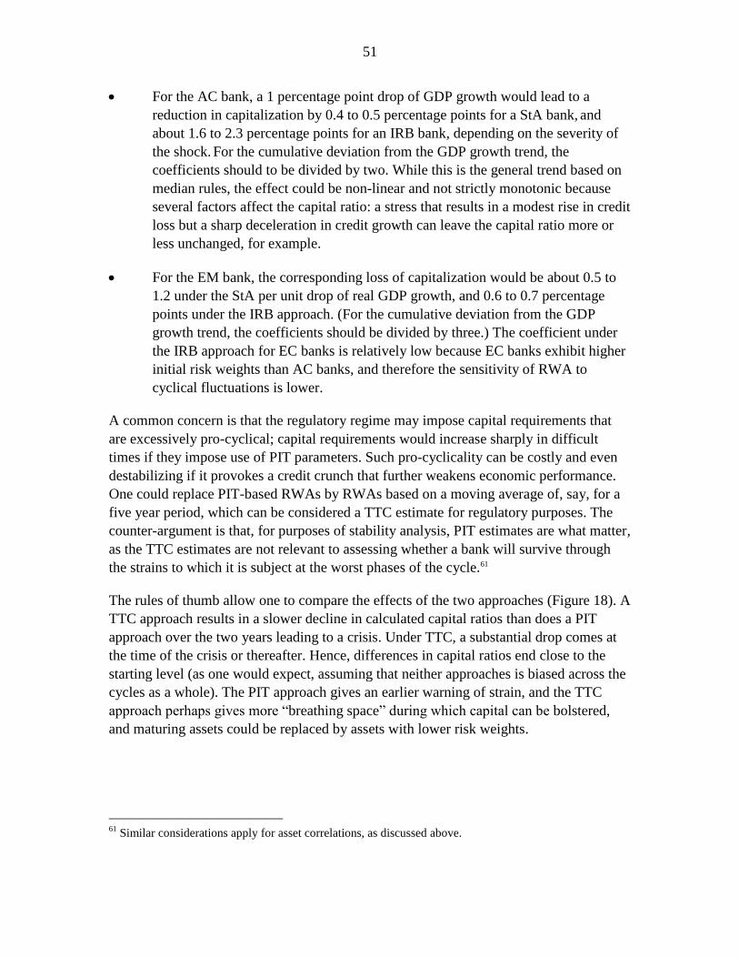
51
For the AC bank, a 1 percentage point drop of GDP growth would lead to a
reduction in capitalization by 0.4 to 0.5 percentage points for a StA bank, and
about 1.6 to 2.3 percentage points for an IRB bank, depending on the severity of
the shock. For the cumulative deviation from the GDP growth trend, the
coefficients should to be divided by two. While this is the general trend based on
median rules, the effect could be non-linear and not strictly monotonic because
several factors affect the capital ratio: a stress that results in a modest rise in credit
loss but a sharp deceleration in credit growth can leave the capital ratio more or
less unchanged, for example.
For the EM bank, the corresponding loss of capitalization would be about 0.5 to
1.2 under the StA per unit drop of real GDP growth, and 0.6 to 0.7 percentage
points under the IRB approach. (For the cumulative deviation from the GDP
growth trend, the coefficients should be divided by three.) The coefficient under
the IRB approach for EC banks is relatively low because EC banks exhibit higher
initial risk weights than AC banks, and therefore the sensitivity of RWA to
cyclical fluctuations is lower.
A common concern is that the regulatory regime may impose capital requirements that
are excessively pro-cyclical; capital requirements would increase sharply in difficult
times if they impose use of PIT parameters. Such pro-cyclicality can be costly and even
destabilizing if it provokes a credit crunch that further weakens economic performance.
One could replace PIT-based RWAs by RWAs based on a moving average of, say, for a
five year period, which can be considered a TTC estimate for regulatory purposes. The
counter-argument is that, for purposes of stability analysis, PIT estimates are what matter,
as the TTC estimates are not relevant to assessing whether a bank will survive through
the strains to which it is subject at the worst phases of the cycle.61
The rules of thumb allow one to compare the effects of the two approaches (Figure 18). A
TTC approach results in a slower decline in calculated capital ratios than does a PIT
approach over the two years leading to a crisis. Under TTC, a substantial drop comes at
the time of the crisis or thereafter. Hence, differences in capital ratios end close to the
starting level (as one would expect, assuming that neither approaches is biased across the
cycles as a whole). The PIT approach gives an earlier warning of strain, and the TTC
approach perhaps gives more “breathing space” during which capital can be bolstered,
and maturing assets could be replaced by assets with lower risk weights.
61
Similar considerations apply for asset correlations, as discussed above.
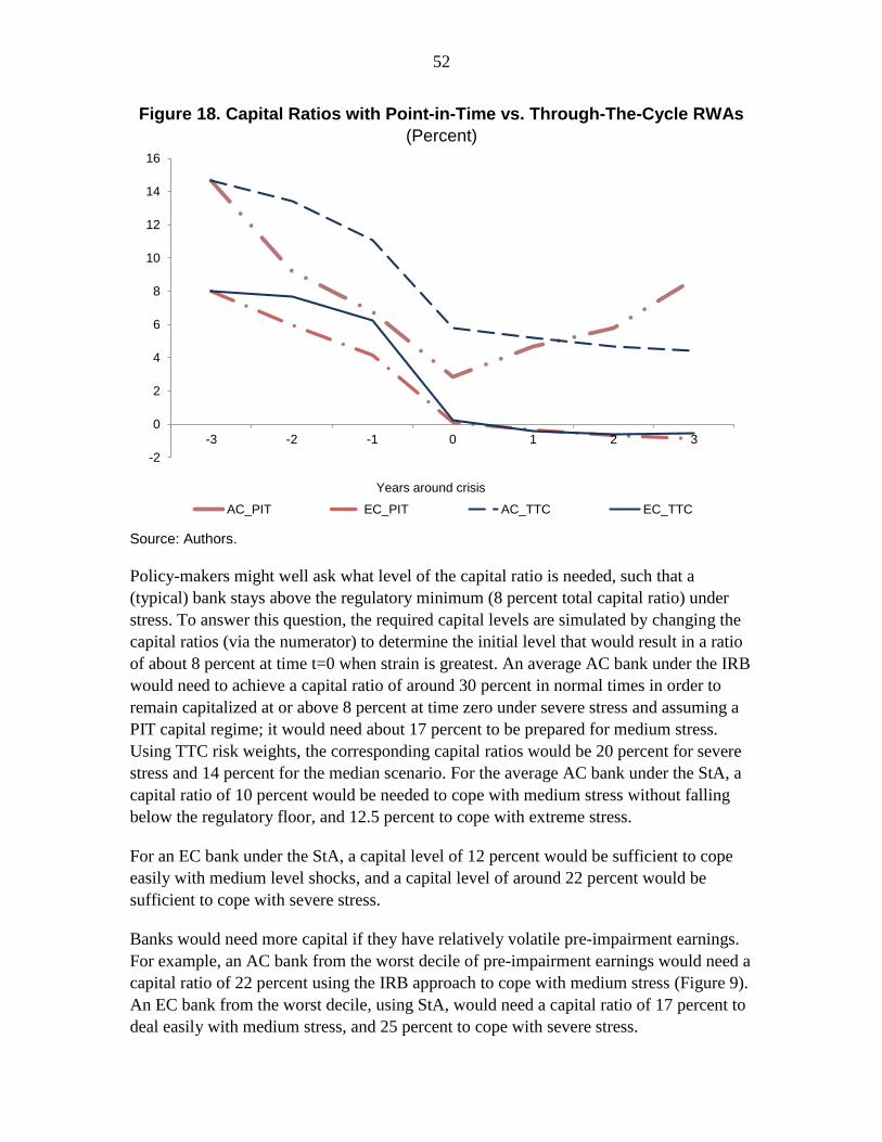
52
Figure 18. Capital Ratios with Point-in-Time vs. Through-The-Cycle RWAs
(Percent)
Source: Authors.
Policy-makers might well ask what level of the capital ratio is needed, such that a
(typical) bank stays above the regulatory minimum (8 percent total capital ratio) under
stress. To answer this question, the required capital levels are simulated by changing the
capital ratios (via the numerator) to determine the initial level that would result in a ratio
of about 8 percent at time t=0 when strain is greatest. An average AC bank under the IRB
would need to achieve a capital ratio of around 30 percent in normal times in order to
remain capitalized at or above 8 percent at time zero under severe stress and assuming a
PIT capital regime; it would need about 17 percent to be prepared for medium stress.
Using TTC risk weights, the corresponding capital ratios would be 20 percent for severe
stress and 14 percent for the median scenario. For the average AC bank under the StA, a
capital ratio of 10 percent would be needed to cope with medium stress without falling
below the regulatory floor, and 12.5 percent to cope with extreme stress.
For an EC bank under the StA, a capital level of 12 percent would be sufficient to cope
easily with medium level shocks, and a capital level of around 22 percent would be
sufficient to cope with severe stress.
Banks would need more capital if they have relatively volatile pre-impairment earnings.
For example, an AC bank from the worst decile of pre-impairment earnings would need a
capital ratio of 22 percent using the IRB approach to cope with medium stress (Figure 9).
An EC bank from the worst decile, using StA, would need a capital ratio of 17 percent to
deal easily with medium stress, and 25 percent to cope with severe stress.
-2
0
2
4
6
8
10
12
14
16
-3 -2 -1 0 1 2 3
Years around crisis
AC_PIT EC_PIT AC_TTC EC_TTC
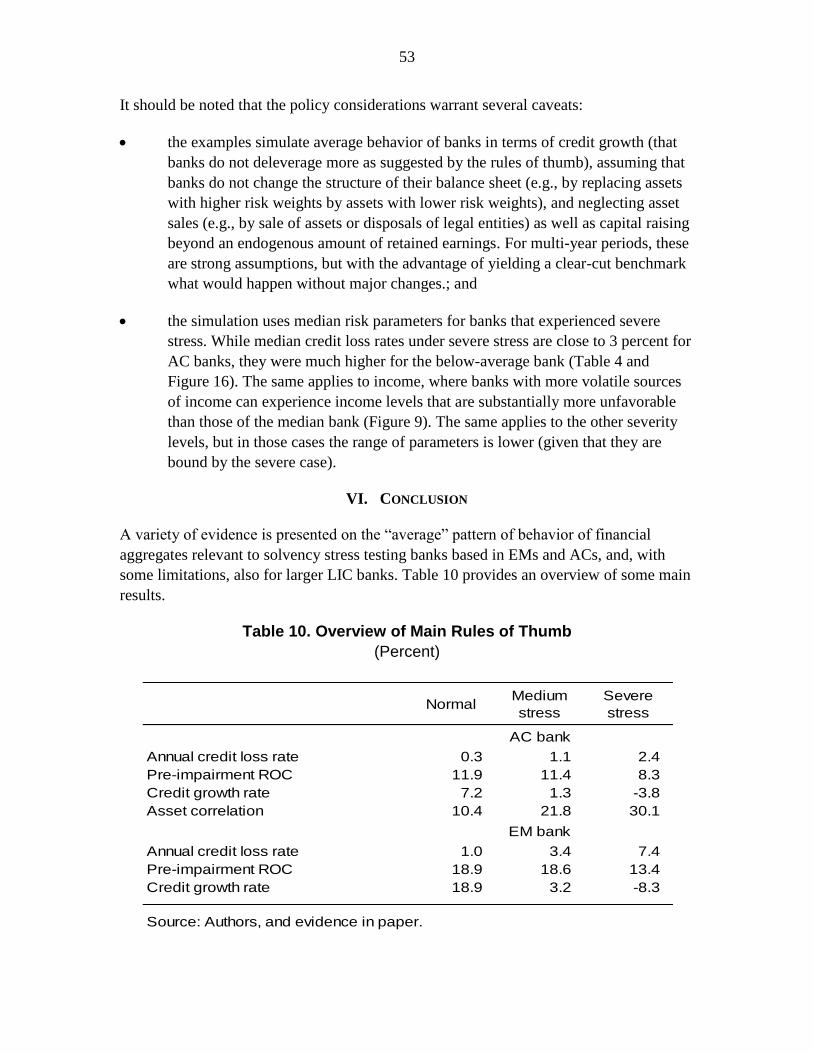
53
It should be noted that the policy considerations warrant several caveats:
the examples simulate average behavior of banks in terms of credit growth (that
banks do not deleverage more as suggested by the rules of thumb), assuming that
banks do not change the structure of their balance sheet (e.g., by replacing assets
with higher risk weights by assets with lower risk weights), and neglecting asset
sales (e.g., by sale of assets or disposals of legal entities) as well as capital raising
beyond an endogenous amount of retained earnings. For multi-year periods, these
are strong assumptions, but with the advantage of yielding a clear-cut benchmark
what would happen without major changes.; and
the simulation uses median risk parameters for banks that experienced severe
stress. While median credit loss rates under severe stress are close to 3 percent for
AC banks, they were much higher for the below-average bank (Table 4 and
Figure 16). The same applies to income, where banks with more volatile sources
of income can experience income levels that are substantially more unfavorable
than those of the median bank (Figure 9). The same applies to the other severity
levels, but in those cases the range of parameters is lower (given that they are
bound by the severe case).
VI. CONCLUSION
A variety of evidence is presented on the “average” pattern of behavior of financial
aggregates relevant to solvency stress testing banks based in EMs and ACs, and, with
some limitations, also for larger LIC banks. Table 10 provides an overview of some main
results.
Table 10. Overview of Main Rules of Thumb
(Percent)
NormalMedium
stress
Severe
stress
AC bank
Annual credit loss rate 0.3 1.1 2.4
Pre-impairment ROC 11.9 11.4 8.3
Credit growth rate 7.2 1.3 -3.8
Asset correlation 10.4 21.8 30.1
EM bank
Annual credit loss rate 1.0 3.4 7.4
Pre-impairment ROC 18.9 18.6 13.4
Credit growth rate 18.9 3.2 -8.3
Source: Authors, and evidence in paper.
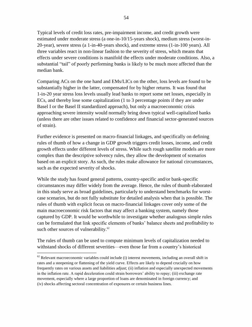
54
Typical levels of credit loss rates, pre-impairment income, and credit growth were
estimated under moderate stress (a one-in-10/15-years shock), medium stress (worst-in-
20-year), severe stress (a 1-in-40-years shock), and extreme stress (1-in-100 years). All
three variables react in non-linear fashion to the severity of stress, which means that
effects under severe conditions is manifold the effects under moderate conditions. Also, a
substantial “tail” of poorly performing banks is likely to be much more affected than the
median bank.
Comparing ACs on the one hand and EMs/LICs on the other, loss levels are found to be
substantially higher in the latter, compensated for by higher returns. It was found that
1-in-20 year stress loss levels usually lead banks to report some net losses, especially in
ECs, and thereby lose some capitalization (1 to 3 percentage points if they are under
Basel I or the Basel II standardized approach), but only a macroeconomic crisis
approaching severe intensity would normally bring down typical well-capitalized banks
(unless there are other issues related to confidence and financial sector-generated sources
of strain).
Further evidence is presented on macro-financial linkages, and specifically on defining
rules of thumb of how a change in GDP growth triggers credit losses, income, and credit
growth effects under different levels of stress. While such rough satellite models are more
complex than the descriptive solvency rules, they allow the development of scenarios
based on an explicit story. As such, the rules make allowance for national circumstances,
such as the expected severity of shocks.
While the study has found general patterns, country-specific and/or bank-specific
circumstances may differ widely from the average. Hence, the rules of thumb elaborated
in this study serve as broad guidelines, particularly to understand benchmarks for worst-
case scenarios, but do not fully substitute for detailed analysis when that is possible. The
rules of thumb with explicit focus on macro-financial linkages cover only some of the
main macroeconomic risk factors that may affect a banking system, namely those
captured by GDP. It would be worthwhile to investigate whether analogous simple rules
can be formulated that link specific elements of banks’ balance sheets and profitability to
such other sources of vulnerability.62
The rules of thumb can be used to compute minimum levels of capitalization needed to
withstand shocks of different severities—even those far from a country’s historical
62
Relevant macroeconomic variables could include (i) interest movements, including an overall shift in
rates and a steepening or flattening of the yield curve. Effects are likely to depend crucially on how
frequently rates on various assets and liabilities adjust; (ii) inflation and especially unexpected movements
in the inflation rate. A rapid deceleration could strain borrowers’ ability to repay; (iii) exchange rate
movement, especially where a large proportion of loans are denominated in foreign currency; and
(iv) shocks affecting sectoral concentration of exposures or certain business lines.
54
55
experience. Also, the regulatory approach used by banks matters: whether a bank adopts
an IRB approach to estimating risk-weighted assets or relies on a standardized approach
is shown to make a substantial difference to the magnitude and also the timing of when
the effects of shocks are recognized, provided that banks’ risk models reflect changes in
risk on a timely basis. Thus, the results are relevant to recent policy discussions centered
on the robustness of regulatory capital ratios, especially on the computation of RWAs
(e.g., BIS 2013, BCBS 2013, Haldane 2012, 2013) and the design of (countercyclical)
capital buffers (e.g., Drehmann and other 2009). The results echo the call for (much)
longer samples to be used in the calibration of models used for RWA computation and
the “right” choice of the regulatory capital ratio (e.g., BCBS 2013, BIS 2013).

56
APPENDIX 1. DATA SUMMARY
Appendix Table 1. Overview of Bankscope Data
Type of country
Number of countries
Number of banks
Assets (US$ trillions)
Original Raw Data
AC 33 13,271 120.4
EM 109 3,126 28.2
LIC 59 543 1.2
Total 201 16,940 149.9
Cleaned, final data
AC 32 9,372 68.8
EM 90 1,131 10.4
LIC 47 206 0.3 Total 169 10,709 79.5
Source: Authors, based on Bankscope data.
Appendix Figure 1. Overview of Raw Bankscope Sample Size by Year
(Number of banks)
Source: Authors, based on Bankscope data.
0
2,000
4,000
6,000
8,000
10,000
12,000
14,000
16,000
18,000
Sample size (Number of banks)
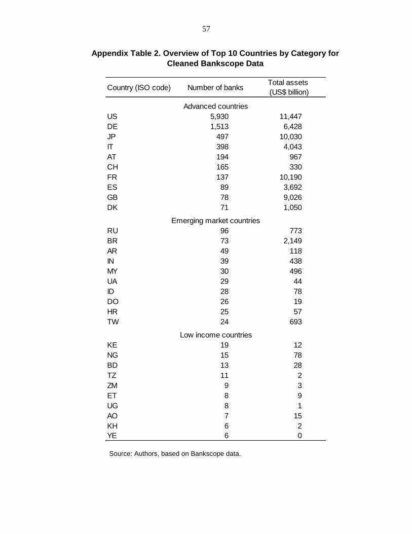
57
Appendix Table 2. Overview of Top 10 Countries by Category for
Cleaned Bankscope Data
Source: Authors, based on Bankscope data.
Country (ISO code) Number of banks Total assets
(US$ billion)
Advanced countries
US 5,930 11,447
DE 1,513 6,428
JP 497 10,030
IT 398 4,043
AT 194 967
CH 165 330
FR 137 10,190
ES 89 3,692
GB 78 9,026
DK 71 1,050
Emerging market countries
RU 96 773
BR 73 2,149
AR 49 118
IN 39 438
MY 30 496
UA 29 44
ID 28 78
DO 26 19
HR 25 57
TW 24 693
Low income countries
KE 19 12
NG 15 78
BD 13 28
TZ 11 2
ZM 9 3
ET 8 9
UG 8 1
AO 7 15
KH 6 2
YE 6 0
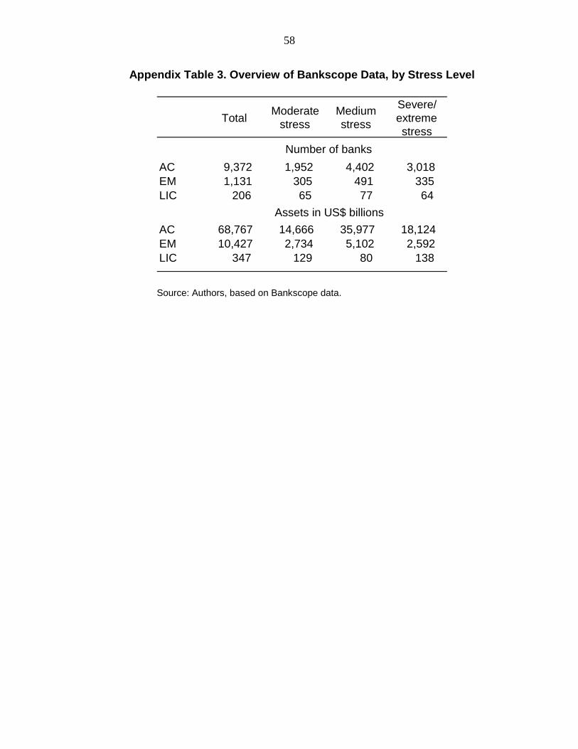
58
Appendix Table 3. Overview of Bankscope Data, by Stress Level
Source: Authors, based on Bankscope data.
Total Moderate
stress
Medium
stress
Severe/
extreme
stress
Number of banks
AC 9,372 1,952 4,402 3,018
EM 1,131 305 491 335
LIC 206 65 77 64
Assets in US$ billions
AC 68,767 14,666 35,977 18,124
EM 10,427 2,734 5,102 2,592
LIC 347 129 80 138

59
APPENDIX 2. SUPPLEMENTARY EVIDENCE
Appendix Table 4. Evolution of Solvency Parameters around Crisis Dates
Years around crisis
-3 -2 -1 0 1 2 3
Credit loss rates/total customer loans
AC "Normal" 0.3 0.3 0.3 0.3 0.3 0.3 0.3
AC Moderate 0.2 0.2 0.4 0.8 0.4 0.3 0.2
AC Medium 0.3 0.4 0.7 1.5 0.7 0.5 0.5
AC Severe 0.3 0.5 1.2 4.0 1.3 0.7 0.5
EM "Normal" 1.0 1.0 1.0 1.0 1.0 1.0 1.0
EM Moderate 0.7 0.8 1.2 2.5 1.2 0.9 0.7
EM Medium 1.1 1.3 2.3 5.2 2.0 1.2 0.9
EM Severe 2.1 2.4 4.1 15.6 3.5 1.8 1.1
LIC "Normal" 1.4 1.4 1.4 1.4 1.4 1.4 1.4
LIC Moderate 1.3 1.2 1.6 3.2 1.2 1.0 0.8
LIC Medium 1.4 0.9 2.1 6.4 1.9 1.2 1.0
LIC Severe 2.8 3.7 3.0 15.3 4.1 1.3 1.7
Credit growth (adjusted for losses)
AC "Normal" 7.2 7.2 7.2 7.2 7.2 7.2 7.2
AC Moderate 7.5 7.5 6.0 3.5 3.2 3.8 4.7
AC Medium 7.0 6.3 4.2 1.3 1.2 2.5 4.0
AC Severe 11.0 8.9 3.6 -3.8 -4.3 -0.3 2.6
EM "Normal" 22.7 22.7 22.7 22.7 22.7 22.7 22.7
EM Moderate 19.8 21.8 19.3 11.8 14.4 18.3 22.7
EM Medium 29.8 26.9 16.1 7.8 13.8 21.8 24.3
EM Severe 23.8 20.1 11.6 1.3 15.5 24.9 23.6
LIC "Normal" 20.5 20.5 20.5 20.5 20.5 20.5 20.5
LIC Moderate 13.3 30.0 36.2 22.0 21.8 28.8 21.4
LIC Medium 31.7 17.1 23.9 12.3 14.9 26.2 23.4
LIC Severe 19.8 20.5 24.5 13.0 15.5 30.3 20.7
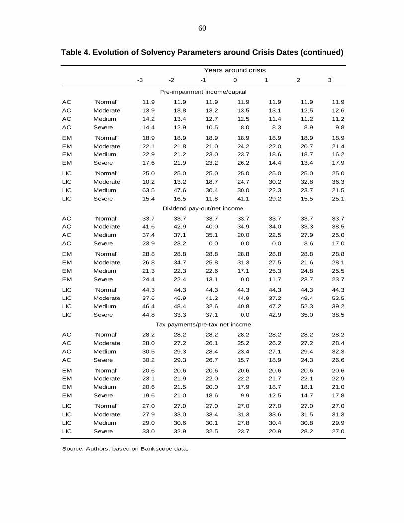
60
Table 4. Evolution of Solvency Parameters around Crisis Dates (continued)
Years around crisis
-3 -2 -1 0 1 2 3
Pre-impairment income/capital
AC "Normal" 11.9 11.9 11.9 11.9 11.9 11.9 11.9
AC Moderate 13.9 13.8 13.2 13.5 13.1 12.5 12.6
AC Medium 14.2 13.4 12.7 12.5 11.4 11.2 11.2
AC Severe 14.4 12.9 10.5 8.0 8.3 8.9 9.8
EM "Normal" 18.9 18.9 18.9 18.9 18.9 18.9 18.9
EM Moderate 22.1 21.8 21.0 24.2 22.0 20.7 21.4
EM Medium 22.9 21.2 23.0 23.7 18.6 18.7 16.2
EM Severe 17.6 21.9 23.2 26.2 14.4 13.4 17.9
LIC "Normal" 25.0 25.0 25.0 25.0 25.0 25.0 25.0
LIC Moderate 10.2 13.2 18.7 24.7 30.2 32.8 36.3
LIC Medium 63.5 47.6 30.4 30.0 22.3 23.7 21.5
LIC Severe 15.4 16.5 11.8 41.1 29.2 15.5 25.1
Dividend pay-out/net income
AC "Normal" 33.7 33.7 33.7 33.7 33.7 33.7 33.7
AC Moderate 41.6 42.9 40.0 34.9 34.0 33.3 38.5
AC Medium 37.4 37.1 35.1 20.0 22.5 27.9 25.0
AC Severe 23.9 23.2 0.0 0.0 0.0 3.6 17.0
EM "Normal" 28.8 28.8 28.8 28.8 28.8 28.8 28.8
EM Moderate 26.8 34.7 25.8 31.3 27.5 21.6 28.1
EM Medium 21.3 22.3 22.6 17.1 25.3 24.8 25.5
EM Severe 24.4 22.4 13.1 0.0 11.7 23.7 23.7
LIC "Normal" 44.3 44.3 44.3 44.3 44.3 44.3 44.3
LIC Moderate 37.6 46.9 41.2 44.9 37.2 49.4 53.5
LIC Medium 46.4 48.4 32.6 40.8 47.2 52.3 39.2
LIC Severe 44.8 33.3 37.1 0.0 42.9 35.0 38.5
Tax payments/pre-tax net income
AC "Normal" 28.2 28.2 28.2 28.2 28.2 28.2 28.2
AC Moderate 28.0 27.2 26.1 25.2 26.2 27.2 28.4
AC Medium 30.5 29.3 28.4 23.4 27.1 29.4 32.3
AC Severe 30.2 29.3 26.7 15.7 18.9 24.3 26.6
EM "Normal" 20.6 20.6 20.6 20.6 20.6 20.6 20.6
EM Moderate 23.1 21.9 22.0 22.2 21.7 22.1 22.9
EM Medium 20.6 21.5 20.0 17.9 18.7 18.1 21.0
EM Severe 19.6 21.0 18.6 9.9 12.5 14.7 17.8
LIC "Normal" 27.0 27.0 27.0 27.0 27.0 27.0 27.0
LIC Moderate 27.9 33.0 33.4 31.3 33.6 31.5 31.3
LIC Medium 29.0 30.6 30.1 27.8 30.4 30.8 29.9
LIC Severe 33.0 32.9 32.5 23.7 20.9 28.2 27.0
Source: Authors, based on Bankscope data.
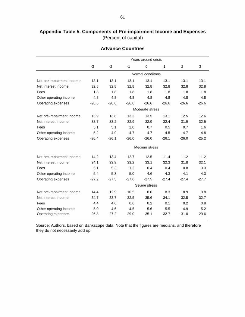
61
Appendix Table 5. Components of Pre-impairment Income and Expenses
(Percent of capital)
Advance Countries
Source: Authors, based on Bankscope data. Note that the figures are medians, and therefore
they do not necessarily add up.
Years around crisis
-3 -2 -1 0 1 2 3
Normal condiitons
Net pre-impairment income 13.1 13.1 13.1 13.1 13.1 13.1 13.1
Net interest income 32.8 32.8 32.8 32.8 32.8 32.8 32.8
Fees 1.8 1.8 1.8 1.8 1.8 1.8 1.8
Other operating income 4.8 4.8 4.8 4.8 4.8 4.8 4.8
Operating expenses -26.6 -26.6 -26.6 -26.6 -26.6 -26.6 -26.6
Moderate stress
Net pre-impairment income 13.9 13.8 13.2 13.5 13.1 12.5 12.6
Net interest income 33.7 33.2 32.9 32.9 32.4 31.9 32.5
Fees 5.1 5.1 2.0 0.7 0.5 0.7 1.6
Other operating income 5.2 4.9 4.7 4.7 4.5 4.7 4.8
Operating expenses -26.4 -26.1 -26.0 -26.0 -26.1 -26.0 -25.2
Medium stress
Net pre-impairment income 14.2 13.4 12.7 12.5 11.4 11.2 11.2
Net interest income 34.1 33.8 33.2 33.1 32.3 31.8 32.1
Fees 5.1 5.3 1.2 0.4 0.4 0.8 3.3
Other operating income 5.4 5.3 5.0 4.6 4.3 4.1 4.3
Operating expenses -27.2 -27.5 -27.6 -27.5 -27.4 -27.4 -27.7
Severe stress
Net pre-impairment income 14.4 12.9 10.5 8.0 8.3 8.9 9.8
Net interest income 34.7 33.7 32.5 35.6 34.1 32.5 32.7
Fees 4.4 4.6 0.6 0.2 0.1 0.2 0.8
Other operating income 5.0 4.6 4.5 5.6 5.5 4.9 5.2
Operating expenses -26.8 -27.2 -29.0 -35.1 -32.7 -31.0 -29.6
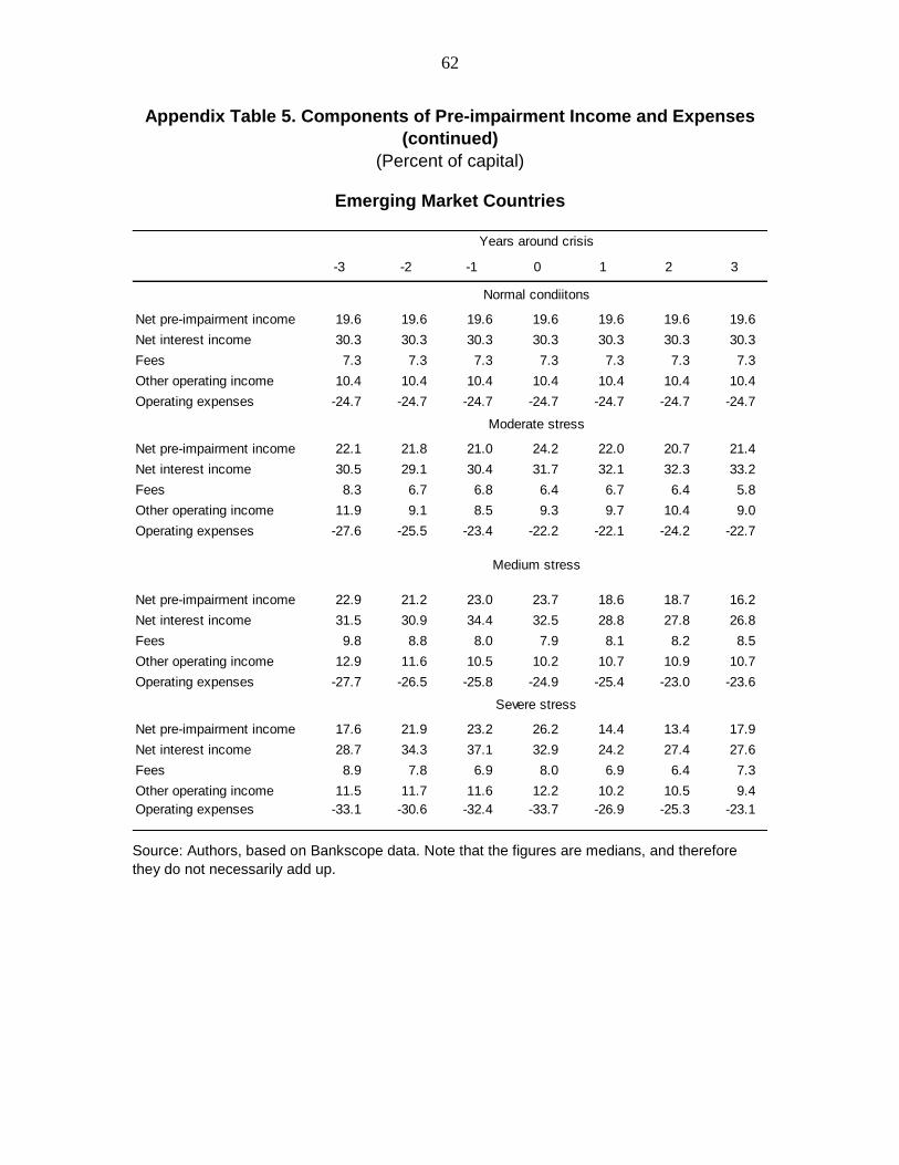
62
Appendix Table 5. Components of Pre-impairment Income and Expenses
(continued)
(Percent of capital)
Emerging Market Countries
Source: Authors, based on Bankscope data. Note that the figures are medians, and therefore
they do not necessarily add up.
Years around crisis
-3 -2 -1 0 1 2 3
Normal condiitons
Net pre-impairment income 19.6 19.6 19.6 19.6 19.6 19.6 19.6
Net interest income 30.3 30.3 30.3 30.3 30.3 30.3 30.3
Fees 7.3 7.3 7.3 7.3 7.3 7.3 7.3
Other operating income 10.4 10.4 10.4 10.4 10.4 10.4 10.4
Operating expenses -24.7 -24.7 -24.7 -24.7 -24.7 -24.7 -24.7
Moderate stress
Net pre-impairment income 22.1 21.8 21.0 24.2 22.0 20.7 21.4
Net interest income 30.5 29.1 30.4 31.7 32.1 32.3 33.2
Fees 8.3 6.7 6.8 6.4 6.7 6.4 5.8
Other operating income 11.9 9.1 8.5 9.3 9.7 10.4 9.0
Operating expenses -27.6 -25.5 -23.4 -22.2 -22.1 -24.2 -22.7
Medium stress
Net pre-impairment income 22.9 21.2 23.0 23.7 18.6 18.7 16.2
Net interest income 31.5 30.9 34.4 32.5 28.8 27.8 26.8
Fees 9.8 8.8 8.0 7.9 8.1 8.2 8.5
Other operating income 12.9 11.6 10.5 10.2 10.7 10.9 10.7
Operating expenses -27.7 -26.5 -25.8 -24.9 -25.4 -23.0 -23.6
Severe stress
Net pre-impairment income 17.6 21.9 23.2 26.2 14.4 13.4 17.9
Net interest income 28.7 34.3 37.1 32.9 24.2 27.4 27.6
Fees 8.9 7.8 6.9 8.0 6.9 6.4 7.3
Other operating income 11.5 11.7 11.6 12.2 10.2 10.5 9.4
Operating expenses -33.1 -30.6 -32.4 -33.7 -26.9 -25.3 -23.1
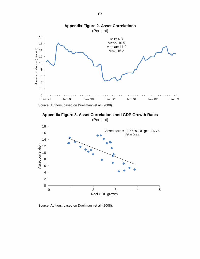
63
Appendix Figure 2. Asset Correlations
(Percent)
Source: Authors, based on Duellmann et al. (2008).
Appendix Figure 3. Asset Correlations and GDP Growth Rates
(Percent)
Source: Authors, based on Duellmann et al. (2008).
0
2
4
6
8
10
12
14
16
18
Jan. 97 Jan. 98 Jan. 99 Jan. 00 Jan. 01 Jan. 02 Jan. 03
Asset co
rrela
tio
n (p
erc
ent)
Min: 4.3Mean: 10.5
Median: 11.2Max: 16.2
Asset corr. = -2.66RGDP gr.+ 16.76R² = 0.44
0
2
4
6
8
10
12
14
16
18
0 1 2 3 4 5
Asse
t co
rre
latio
n
Real GDP growth

64
REFERENCES
Alfaro, Rodrigo, and Matthias Drehmann, 2009, “Macro stress tests and crises: what can
we learn?” BIS Quarterly Review December.
Araten, Michael, Michael Jr. Jakobs and Varshney Peeyush, 2004, “Measuring LGD on
commercial loans: An 18-year internal study,” The RMA Journal, May, pp. 28–
35.
Basel Committee on Banking Supervision (BCBS), 2011, “Basel III: A global regulatory
framework for more resilient banks and banking systems,” revised version, June,
at www.bis.org/publ/bcbs189.pdf.
Basel Committee on Banking Supervision (BCBS), 2013, “Regulatory consistency
assessment programme (RCAP) — Analysis of risk-weighted assets for credit risk
in the banking book,” at www.bis.org/publ/bcbs256.pdf .
Bank of International Settlements (BIS), 2013, “The road to a more resilient banking
sector,” Annual Report, pp. 52–65.
Borio, Claudio, 2012, “The financial cycle and macroeconomics: What have we learnt?”
BIS working paper no. 395.
Borio, Claudio, Matthias Drehmann, and Tsatsaronis Kostas, 2012, “Stress-testing macro
stress testing: does it live up to expectations?,” BIS working paper no. 369.
Čihák, Martin, 2007, “Introduction to Applied Stress Testing,” IMF Working Paper no.
07/59.
Čihák, Martin and Klaus Schaeck, 2007, “How Well Do Aggregate Bank Ratios Identify
Banking Problems?”, IMF Working Paper no. 07/275.
Djankov, Simeon, Caralee McLiesh, and Andrei Shleifer, 2007, “Private credit in 129
countries,” Journal of Financial Economics 84, pp. 299–329.
Drehmann, M., C. Borio, L. Gambacorta, G. Jiminez, and C. Trucharte, 2009,
“Countercyclical capital buffers: exploring options,” BIS Working Papers, no.
317.
Drehmann, Matthias, 2009, “Macroeconomic stress testing banks: a survey of
methodologies,” in: Quagliariello, Mario (ed), Stress testing the banking system:
methodologies and applications, Cambridge University Press.

65
Düllmann, Klaus, Martin Scheicher, and Christian Schmieder, 2008, “Asset correlations
and credit portfolio risk — an empirical analysis,” Journal of Credit Risk 4(2),
pp. 37–62.
European Banking Authority, 2011, “2011 EU-wide Stress Testing Exercise,” at
http://stress-test.eba.europa.eu/.
Federal Reserve Board of Governors, 2009, “Supervisory Capital Assessment Program,”
at http://www.federalreserve.gov/bankinforeg/scap.htm.
Federal Reserve Bank of St. Louis, 2013, Federal Reserve Economic Data, Time Series
for Real Gross Domestic Product (GDPCA), at
http://research.stlouisfed.org/fred2/series/GDPCA?cid=106.
Federal Reserve Board of Governors, 2012, “Comprehensive Capital Analysis and
Review 2012: Methodology and Results for Stress Scenario Projections,” at
http://www.federalreserve.gov/newsevents/press/bcreg/20120313a.htm.
Foglia, Antonella, 2008, “Stress testing credit risk: a survey of authorities' approaches,”
Banca d’Italia, Occasional Papers no. 37.
Giesecke, Kai, Francis A. Longstaff, Stephen Schaefer, and Ilya Strebulaev, 2011,
“Corporate bond default risk: A 150-year perspective,” Journal of Financial
Economics 102, pp. 233–250.
International Monetary Fund, 2010, “Resolution of Cross-Border Banks—A Proposed
Framework for Enhanced Coordination,” at
www.imf.org/external/np/pp/eng/2010/061110.pdf.
International Monetary Fund, 2011a, “Overcoming Political Risks and Crisis Legacies,”
Chapter 1, Global Financial Stability Report, September.
International Monetary Fund, 2011b, “Towards Operationalizing Macroprudential
Policies,” Chapter 3 of the Global Financial Stability Report, September.
Haldane, Andrew G., 2012, “The dog and the Frisbee,” Bank of England speech, at
www.bankofengland.co.uk/publications/Pages/speeches/2012/596.aspx.
Haldane, Andrew G., 2013, “Constraining discretion in bank regulation,” Paper presented
at the Federal Reserve Bank of Atlanta, 9 April 2013, at
www.bankofengland.co.uk/publications/Pages/speeches/2013/657.aspx.
66
Hardy, Daniel C., and Ceyla Pazarbaşioğlu, 1999, “Determinants and Leading Indicators
of Banking Crises: Further Evidence,” IMF Staff Papers 46, pp. 247–258.
Jobst, Andreas, Li Lian Ong, and Christian Schmieder, 2013, “A Framework for
Macroprudential Bank Solvency Stress Testing: Application to S-25 and Other G-
20 Country FSAPs,” IMF Working Paper no. 03/12.
Lo, Andrew W., 2012, “Reading About the Financial Crisis: A 21-Book Review,”
available online at www.argentumlux.org/documents/JEL_6.pdf.
Lopez, Jose A., 2004, “The empirical relationship between average asset correlation, firm
probability of default, and asset size,” Journal of Financial Intermediation 13(2),
pp. 265–283.
Marcucci, Juri, and Mario Quagliariello, 2009, “Asymmetric effects of the business cycle
on bank credit risk,” Journal of Banking and Finance, 33(9), pp. 1624–1635.
Moody’s, 2013, “Corporate Default and Recovery Rates, 1920–2012,” Special Comment,
February.
Schmieder, Christian, Heiko Hesse, Benjamin Neudorfer, Claus Puhr, and Stefan W.
Schmitz, 2012, “Next Generation System-Wide Liquidity Stress Testing,” IMF
Working Paper no. 03/12.
Schmieder, Christian, Claus Puhr, and Maher Hasan, 2011, “Next Generation Balance
Sheet Based Stress Testing”, IMF Working Paper no. 11/83.
Schmieder, Christian, and S. Philipp Schmieder, 2011, “Impact of Legislation on Credit
Risk—Comparative Evidence from the United States, the United Kingdom, and
Germany,” IMF Working Paper no. 11/55.
Taleb, Nassim N., Elie Canetti, Tidiane Kinda, Elena Loukoianova, and Christian
Schmieder, 2012, “A New Heuristic Measure of Fragility and Tail Risks:
Application to Stress Testing,” IMF Working Paper no. 12/216.
Taleb, Nassim N., 2010, “The Black Swan—The Impact of the Highly Improbable,”
Revised Edition. Random House, New York.


