
ROTOR-BEARING SYSTEM DYNAMICS OF A HIGH
SPEED MICRO END MILL SPINDLE
By
VUGAR SAMADLI
A THESIS PRESENTED TO THE GRADUATE SCHOOL OF THE UNIVERSITY OF FLORIDA IN PARTIAL FULFILLMENT
OF THE REQUIREMENTS FOR THE DEGREE OF MASTER OF SCIENCE
UNIVERSITY OF FLORIDA
2006

Copyright 2006
by
Vugar Samadli

iii
ACKNOWLEDGMENTS
I would like to first thank my advisor, Dr. N. Arakere, for guiding me through this
work. I feel that I have learned much working on this project and that would not have
been possible without his help. Similarly, the collaboration with Dr. J. Zeigert and Dr. L.
William and their students Scott Payne, Eric Major and Andrew Riggs was fruitful. I
want to thank Scott Payne for his help and it was always a friendly environment to work
with him in his lab.
My company, BP Azerbaijan unit, was a main factor in making this whole effort
possible so I would like to thank them all, and specifically Ralph Ladd, learning and
development coordinator, and Kevin Kennelley, engineering manager.
Lastly, I would like to thank my parents because they were supportive of this
effort and always encouraged my education.

iv
TABLE OF CONTENTS page
ACKNOWLEDGMENTS ................................................................................................. iii
LIST OF TABLES............................................................................................................. vi
LIST OF FIGURES .......................................................................................................... vii
ABSTRACT....................................................................................................................... ix
CHAPTER
1 INTRODUCTION ........................................................................................................1
2 DEVELOPMENT OF EQUATION OF MOTION OF ROTOR-BEARING SYSTEM AND PARAMETER IDENTIFICATION...................................................4
2.1 Rigid Rotor Analysis ..............................................................................................4 2.2 Finite Element Analysis..........................................................................................7 2.3 Identifying Bearing Parameters By Experimental Method ....................................8
2.3.1 Methods Using Incremental Static Load...............................................9 2.3.2 Methods Using Dynamic Load .............................................................9 2.3.3 Methods Using an Excitation Force ....................................................11 2.3.4 Method Using Unbalance Mass ..........................................................14 2.3.5 Methods Using an Impact Hammer ....................................................16 2.3.6 Methods Using Unknown Excitation ..................................................17
3 ROTOR DYNAMIC ANALYSIS OF MICRO SPINDLE ........................................19
3.1 Rigid Rotor Analysis ............................................................................................20 3.2 Finite Element Analysis........................................................................................31 3.3 Summary...............................................................................................................42
4 EXPERIMENTAL IDENTIFICATION OF BEARING PARAMETERS ................44
4.1 Method of Measurement.......................................................................................45 4.2 Design Process......................................................................................................48
5 CONCLUSION AND RECOMMENDATIONS .......................................................50

v
APPENDIX
A CHRONOLOGICAL LIST OF PAPERS ON THE EXPERIMENTAL DYNAMIC PARAMETER IDENTIFICATION OF BEARINGS............................51
B GENERAL RIGID ROTOR SOLUTION 1 ...............................................................55
C GENERAL RIGID ROTOR SOLUTION 2 ...............................................................62
D EXAMPLE OF FINDING BEARING PARAMETERS............................................69
E KISTLER DYNANOMETER....................................................................................72
LIST OF REFERENCES...................................................................................................74
BIOGRAPHICAL SKETCH .............................................................................................77

vi
LIST OF TABLES
Table page 3-1 Bearing parameters at 500,000 rpm (Ω=52360 rad/sec). .........................................23
3-2 Bearing Parameters for different rotor speeds..........................................................29

vii
LIST OF FIGURES
Figure page 1-1 Commercial micro-tool ..............................................................................................3
2-1 Rigid rotor schematic. ................................................................................................5
2-2 A non-floating bearing housing and a rotating journal. ...........................................11
2-3 A floating bearing housing and a fixed rotating shaft. .............................................12
3-1 Micro-spindle. .........................................................................................................20
3-2 Bearings location on spindle. ...................................................................................20
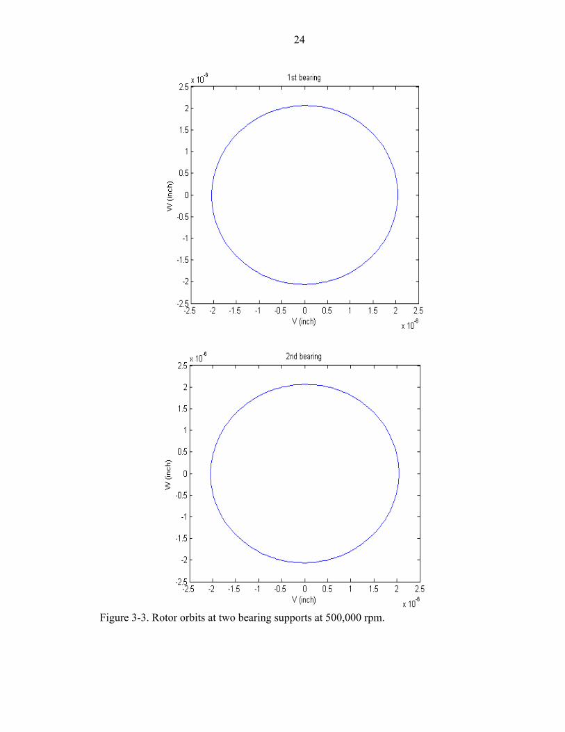
3-3 Rotor orbits at two bearing supports at 500,000 rpm. ..............................................24
3-4 Rotor orbits at the two bearing supports at 1,000,000 rpm. .....................................25
3-5 Rotor orbits at the tool end at 500,000 rpm..............................................................26
3-6 Orbit amplitude at 1st, 2nd bearing and tool tip. ........................................................27
3-7 Stiffness, Kyy versus rotor eccentricity. ..................................................................28
3-8 Whirl map.................................................................................................................30
3-9 Finite element model. ...............................................................................................31
3-10 Rigid body mode 1, 107758 rpm..............................................................................31
3-11 Rotor analysis at 115298 rpm. A) Rigid body mode 2, B) Potential energy distribution. ..............................................................................................................32
3-12 Rotor analysis at 2,042,349 rpm. A) Flexural mode 1, B) potential energy distribution. ..............................................................................................................32
3-13 Flexural mode 2, 4,955,776 rpm. .............................................................................33
3-14 Critical speed map. ...................................................................................................33

viii
3-15 1st bearing. A) and B) Unbalance response, C) Amplitude and phase lag, D) Nyquist plot for displacement. .................................................................................34
3-16 2nd bearing. A) and B) Unbalance response, C) Amplitude and phase lag, D) Nyquist plot for displacement. .................................................................................36
3-17 Tool tip. A) Unbalance response, B) Amplitude and phase lag, C) Nyquist plot for displacement. ......................................................................................................38
3-18 Shaft orbits. A), B), C), D), E), F) are shaft orbits as a function of speed. ..............39
3-19 Stability Map (Note: Negative log decrements indicate instability). .......................42
3-20 Orbit amplitude at 1st, 2nd bearing and tool tip, є=0.1. .............................................43
4-1 Flexure supported ball bearing: 1) Flexure, 2) Ball bearing. ...................................45
4-2 A chassis...................................................................................................................45
4-3 Schematic of the test rig. ..........................................................................................46
4-4 Test Setup: 1) Base, 2) Dyno, 3) Chassis, 4) Test bearing, 5) Shaft, 6) Spindle .....48
4-5 Main Chassis: 1) Stator, 2) Displacement Probe, 3) Test Bearing...........................49
4-6 Measurment system..................................................................................................49

ix
Abstract of Thesis Presented to the Graduate School
of the University of Florida in Partial Fulfillment of the Requirements for the Degree of Master of Science
ROTOR-BEARING SYSTEM DYNAMICS OF A HIGH SPEED MICRO END MILL SPINDLE
By
Vugar Samadli
August 2006
Chair: Nagaraj Arakere Major Department: Mechanical and Aerospace Engineering
Current micro-scale manufacturing technologies find limited application in a wide
range of high strength engineering materials because of the difficulties encountered in
creating complex three dimensional structures and features. Although milling is one of
the most widely used processes for this type of manufacturing at the macro scale, it has
yet to become an economically viable technology for micro-scale manufacturing. For
optimal chip formation using very small diameter cutters, and to achieve economical
material removal rates combined with good surface finish, high spindle speeds are
needed. In addition, a low runout is desired to prevent premature tool breakage. However,
the lack of suitable spindles capable of achieving rotational speeds in excess of 500,000
rpm coupled with sub-micrometer runout at the tool tip makes micro-scale milling
commercially unviable.

x
This thesis demonstrates several means of analyzing the rotor dynamic behavior of
a spindle in order to find critical speeds, unbalance response and linear stability margins.
Experimental testing is performed to estimate bearing dynamic behavior at high speed.
The results of this study provide parameters for bearing stiffness and damping,
bearing span and balancing limits to achieve sub-micrometer runout of tool tip for speeds
upto 1 million rpm.

1
CHAPTER 1 INTRODUCTION
The technology development in the field of miniaturization has become a global
phenomenon. Its impact is far and widespread across a broad application domain that
encompasses many diverse fields and industries, such as telecommunications, portable
consumer electronics, defense, and biomedical. The perfect example is the field of
computers where modern computers which possess greater processing power and can fit
under a desk or on a lap have replaced the bulky computers of the past such as the
ENIAC (electronic numerical integrator and computer) which once filled large rooms. In
recent times, more and more attention is being paid to the issues involved in the design,
development, operation, and analysis of the equipment and processes of manufacturing
micro components since the global trend toward the increased integration of miniaturized
technology into society has gained enormous momentum. Currently, common techniques
utilized in the fabrication of micro-components are based on the techniques developed for
the silicon wafer processing industry. Unfortunately these processes are limited to
production of simple planar geometries in a narrow range of material and are cost
effective only in large volume [1]. Even though non traditional fabrication methods, such
as focused ion beam machining, laser machining, and electrodischarge machining, are
capable of producing high-precision micro-components, they have limited potential as
mass production techniques due to the high initial cost, poor productivity, and limited
material selection [2]. Micro milling has the potential to fabricate micro components and
is capable of machining complex 3D shapes from wide variety of shapes and materials.

2
The objective of this research is to develop a micro-milling spindle which will rotate at
over 500,000 rpm range with sub-micrometer runout, and thus become a commercially
usable and cost effective manufacturing technology. Most machine tools such as lathes,
milling machines, and all types of grinding machines, use a spindle or an axis of rotation
for positioning work pieces or tools or machining parts and thus a large part of their
accuracy can be attributed to the spindle. Consequently, the accuracy of the spindles used
in their design directly influences the accuracy of the entire machine and thus can be
considered as one of the most important components in the overall accuracy and
operation of a machine tool.
Most commercial micro-tools have a 1/8th inch diameter shank (see Figure 1-1).
This must be of utmost importance when designing the micro spindle. Another functional
requirement is the ease of tool changing with minimal time and effort. The only viable
way to meet the above design requirements while still obtaining satisfactory runout is to
concentrate on designs incorporating the use of tool shank itself as the spindle shaft. To
achieve desired performance, the following three functions must be satisfied:
1. Bearing subsystem. The bearing system must be so designed that it meets the following requirements. Firstly and fore mostly, it must be capable of supporting the tool shank without causing excessive runout. Also, it must support both radial and axial loads, and support rapid tool changes. Flexure Pivot Tilting Pad Bearings (FPTPB) are being studied as a potential bearing subsystem.
2. Drive subsystem. The tool drive system must be able to drive the tool at the required speed with enough torque and power to perform the desired machining operations. Also it should not introduce disturbance forces that cause excessive tool point runout. These requirements make air turbine drive as a potential drive subsystem. The system would incorporate the turbine blades directly into the tool shank of the micro-tool.
3. Monitoring subsystem. Theoretical and scientific understanding of micro-milling requires monitoring and recording of cutting forces. However, in the measurement bandwidth (that is 1,000,000 rpm with a 2-flute cutter and tooth passing frequency

3
of 33 KHz), the force measurement is extremely difficult because of the high frequencies encountered even though the cutting forces are low.
The goals of this project are the following: • To extend the capability to model and predict rotordynamics and bearing behavior at
small sizes and high speeds. • Development of a procedure for identification of dynamic stiffness and damping
coefficients for the bearing.
Figure 1-1. Commercial micro-tool

4
CHAPTER 2 DEVELOPMENT OF EQUATION OF MOTION OF ROTOR-BEARING SYSTEM
AND PARAMETER IDENTIFICATION
It is of utmost importance in many companies that not only the operation should be
uninterrupted and reliable but also it should be carried out at high power and high speed.
Another vital requirement is the accurate prediction and control of the dynamic behavior
(unbalance response, critical speeds and instability). These factors were the motivations
for this research wherein rigid rotor analysis and finite element analysis was used to
investigate bearing coefficient parameters and the rotordynamics of micro spindle. Both
the rigid rotor analysis and finite element analysis have been performed simultaneously.
The tungsten carbide spindle has a first bending or flexure natural frequency of 2.2
million rpm for a bearing span of 1 inch. The spindle operating speeds are expected to be
about 500,000 rpm. Hence rigid rotor analysis can be justified. Finally, the experimental
setup was designed to find bearing parameters which were compared with analytical
results.
2.1 Rigid Rotor Analysis
In order to get generalized rotor dynamic models, the Jeffcott rotor is extended to a
four degree of freedom rigid rotor system as shown in the schematic diagram of Figure 2-
1. The four coordinates, which are the two geometric center translations (V, W) and the
two rotation angles (B, Γ) describe the rotor configuration relative to the fixed reference
(X, Y, Z). Bearing 1 and bearing 2 are located at an axial distance a1 and a2 from the

5
center of mass, respectively. Both these distances are defined as positive in the plus X
direction. The rotor configuration is always defined so that a1 is positive.
Y
ZX
V
Wa1a2
Brg.1
Brg.2
B
ΩΓ
Z
YV
W
m b
c
φ Ω= tη
ζ
Figure 2-1. Rigid rotor schematic.
Where
(a, b, c) geometric center body reference (η, ζ) eccentricity components (φ) spin angle = Ωt (Ω) constant spin frequency
( ) ( cos sin )
( ) ( cos sin )
V t VmW t Wm
η ϕ ζ ϕ
ζ ϕ η ϕ
= + −
= + + (2-1)
The angular rate of the rigid body is
sin
cos sin cos
cos cos sin
a
b
c
t t
t t
ω
ω
ω
= Ω−Γ Β
= Γ Β Ω +Β Ω
= Γ Β Ω −Β Ω
&
& &
& &
(2-2)

6
and the kinetic energy of the rigid body is
1 12 2 2 2 2( ) ( )2 2
T m V W I Im m p a cd bω ω ω⎡ ⎤= + + + +⎢ ⎥⎣ ⎦& &
(2-3)
By considering the variational work of the bearing forces, they are included in the
equation of motion. The bearing force is a function of lateral shaft translations and
velocities at the bearing location.
( , , , )
( , , , )
F F V W V WY YF F V W V WZ Z
=
=
& &
& & (2-4)
Upon Taylor’s series expansion of eq. (2-4) about the origin, the force
components in eq. (2-4) are approximated by their corresponding linear forms. At the ith
typical bearing, forces are expressed in the following equation:
k k c cF V ViYY iYZ i iYY iYZY iF k k W c c WiZ iZY iZZ iZY iZZ i
⎡ ⎤⎡ ⎤ ⎡ ⎤⎡ ⎤ ⎡ ⎤= − − ⎢ ⎥⎢ ⎥ ⎢ ⎥⎢ ⎥ ⎢ ⎥
⎢ ⎥⎢ ⎥ ⎢ ⎥⎢ ⎥ ⎢ ⎥⎣ ⎦⎣ ⎦ ⎣ ⎦ ⎣ ⎦ ⎣ ⎦
&
& (2-5a)
or
F k r c ri i i i i= − − &
(2-5b)
where
1 0 0
0 1 0
air q A qi iai
−⎡ ⎤= =⎢ ⎥⎢ ⎥⎣ ⎦ (2-6)
. [ ]Tq V W B= Γ (2-7)
The variational work done by bearing forces on the rotor is given by the following
expression
2 4
1 1W F r Q qi ik k ki kδ δ δ= =∑ ∑
= = (2-8)
where Qk represents the generalized bearing forces.

7
Lagrange’s equations are of the following form:
( )d T T Qkdt q qk k
∂ ∂− =
∂ ∂& k=1,2,3,4 (2-9)
Using the above set of equations and inserting in eq (2-9) the following set of rigid
rotor equations of motion has been obtained:
( )Mq C G q Kq Q+ −Ω + =&& & (2-10)
where
0 0 00 0 00 0 0
0 0 0
mm
M IdId
⎡ ⎤⎢ ⎥⎢ ⎥= ⎢ ⎥⎢ ⎥⎢ ⎥⎣ ⎦
0 0 0 00 0 0 00 0 0
0 0 0
G I pI p
⎡ ⎤⎢ ⎥⎢ ⎥= ⎢ ⎥−⎢ ⎥⎢ ⎥⎣ ⎦
2
1TK A k Ai i ii
= ∑=
2
1TC A c Ai i ii
= ∑=
2 2cos sin0 00 0
Q m t m t
η ζζ η
−⎡ ⎤ ⎡ ⎤⎢ ⎥ ⎢ ⎥⎢ ⎥ ⎢ ⎥= Ω Ω + Ω Ω⎢ ⎥ ⎢ ⎥⎢ ⎥ ⎢ ⎥⎣ ⎦ ⎣ ⎦ (2-11)
2.2 Finite Element Analysis
Typically, it is not possible to obtain analytical solutions for problems involving
complicated geometries, loadings and material properties. Based on the study and
inspection of various approaches available for modeling, one of the most appropriate
methods for modeling of high-speed micro spindle is the FEA, finite element method. It
is also the only feasible type of computer simulation available for this purpose. The finite
element method is generally a numerical method used for solving engineering and
mathematical physics problems. The following steps are used in the FEA for dynamic
response solution [3]:

8
• Form element stiffness matrix.
• Form element mass matrix.
• Assemble system stiffness matrix and incorporate constraints.
• Assemble system mass matrix and incorporate constraints.
• Solve eigenproblem and obtain a vector of frequencies and mode shapes.
• Form excitation vector in physical coordinates.
2.3 Identifying Bearing Parameters By Experimental Method
The estimation of the dynamic bearing characteristics using theoretical methods
usually results in an error in the prediction of the dynamic behavior of rotor-bearing
systems. Reliable estimates of the bearing operating condition in actual test conditions
are difficult to obtain and, therefore to reduce the discrepancy between the measurements
and the prediction, physically meaningful and accurate parameter identification is
required in actual test conditions. There are some similarities between various
experimental methods for the dynamic characterization of rolling element bearings, fluid-
film bearings and magnetic bearings. These methods require forces as input signals and
displacement/velocities/accelerations of the dynamic system to be measured are usually
the output signals, and input-output relationships are used to determine the unknown
parameters of the system models. There are a lot of identification techniques of bearing
parameters, which are based on methods used to excite the system [4], such as the
following:
1. Methods using Incremental Static Load
2. Methods using Dynamic Load
3. Methods using an Excited Load
4. Method using Unbalance Mass

9
5. Methods using an Impact Hammer
6. Methods using Unknown Excitation
Appendix A summarizes the source material on the experimental dynamic
parameter identification of bearings.
2.3.1 Methods Using Incremental Static Load
Mitchell et al. (1965-66) [5] performed experiments to incrementally load the
bearing and measuring the change in position, and obtained the four stiffness coefficients
of fluid-film bearings. They obtained the following simple relationships using the
influence coefficient approach to
/
/
k zzyykzy zy
α γ
α γ
=
= −
/
/
kyz yzkzz yy
α γ
α γ
= −
= (2-12)
where
zzyy yz zyγ α α α α= −
/1/2
y Fyy yy Fzyz
α
α
= ∆
= ∆
/1/2
z Fzy yz Fzz z
α
α
= ∆
= ∆ (2-13)
Here y1 and z1 are displacements of the journal center from its static equilibrium
position in vertical and horizontal directions respectively, on the application of a static
incremental load Fy∆ in the vertical direction; and y2 and z2 are displacements
corresponding to a static incremental load Fz∆ in the horizontal direction. This method
can be applied to any type of bearing since the estimation of stiffness requires the
establishment of a relationship between the force and the corresponding displacement.
2.3.2 Methods Using Dynamic Load
Dynamic load methods have been the most researched and widely used in the
identification of dynamic bearing parameters in the last 45 years [4]. Their major

10
advantages are that they can be readily implemented on a real machine and the excitation
can be applied either to the journal or to the bearing housing depending on practical
constraints.
For the rigid rotor case, when the excitation is applied to the journal (Figure 2-2),
the fluid-film dynamic equation can be written as
m ( )yy
( )
m c c k k f m y yy y yyz yy yz yy yz y Bm m z c c z k k z f m z zzz zz zz zzy zy zy B
− +⎡ ⎤ ⎡ ⎤ ⎡ ⎤ ⎧ ⎫⎧ ⎫ ⎧ ⎫ ⎧ ⎫ ⎪ ⎪+ + =⎢ ⎥ ⎢ ⎥ ⎢ ⎥⎨ ⎬ ⎨ ⎬ ⎨ ⎬ ⎨ ⎬− +⎩ ⎭ ⎩ ⎭ ⎩ ⎭⎢ ⎥ ⎢ ⎥ ⎢ ⎥ ⎪ ⎪⎣ ⎦ ⎣ ⎦ ⎣ ⎦ ⎩ ⎭
&& &&&& &
&& & && && (2-14)
where m is the mass of the journal, y and z represent the motion of the journal center
from its equilibrium position relative to the bearing center, and yB and zB are the
components of the absolute displacement of the bearing center in vertical and horizontal
directions, respectively. In this case, the origin of the coordinate system is assumed to be
at the static equilibrium position, so that gravity does not appear explicitly in the equation
of motion. There will be one equation of this form for each of the bearings and the terms
yB, zB represent the motion of the supporting structure. For the case of a rigid rotor with
bearings on a rigid support, equation (2-14) can be expressed in the form
M q C q K q f M qB B B R+ + = −&& & && (2-15)
The subscripts R and B refer to the rotor and bearings, respectively. On collecting
the terms together, we get
( )M M q C q K q fB R B B+ + + =&& & (2-16)
The overall system mass, damping and stiffness matrices can be formed by adding
the separate contributions of the bearings and rotor in equation (2-16). This form was
used by Arumugam et al. (1995) [6] to extract KB and CB in terms of the known and
measurable quantities such as the rotor model, forcing and corresponding response. The

11
sinusoidal response of a rotor at speed Ω is studied using the modified form of this
equation (2-16), and the response is of the form
j tq Qe Ω= The governing equation of motion is given by
[ ]2 ( )M j C K Q F Z Qu⎡ ⎤− Ω + Ω + = = Ω⎢ ⎥⎣ ⎦ (2-17)
where [Z(Ω)] is the dynamic stiffness matrix, Fu is the unbalance force, and Ω is
the rotational frequency of the rotor.
Fluid
Journal
Non floating bearing housing
fy(t)
fz(t)
Figure 2-2. A non-floating bearing housing and a rotating journal.
2.3.3 Methods Using an Excitation Force
The application of a calibrated force to the journal can only rarely be applied in
practical situations. Glienicke (1966–67) [7] adopted the technique of exciting the
floating bearing bush (housing) sinusoidally in two mutually perpendicular directions
(Figure 2-3) and measuring the amplitude and phase of the resulting motions in each
case. The stiffness and damping coefficients were then calculated from the frequency-
domain equations.

12
Morton (1971) [8] devised a measurement using the receptance coefficient method
procedure for the estimation of the dynamic bearing characteristics. He excited the
lightweight floating bearing bush by using very low forcing frequencies, ω (10 and 15
Hz). Assuming the inertia force due the fluid film and bearing housing masses to be
negligible, and for sinusoidal motion, equation (2-14) may be written as
z z FYyy yz yz z Z Fzzzy z
⎡ ⎤ ⎧ ⎫⎧ ⎫ ⎪ ⎪=⎢ ⎥ ⎨ ⎬ ⎨ ⎬⎪ ⎪⎩ ⎭⎢ ⎥ ⎩ ⎭⎣ ⎦
with (2-18)
z k j cω= +
where Y and Z are complex displacements and Fy and Fz are complex forces in the
vertical and horizontal directions, respectively. In equation (2-18) k represents the
effective bearing stiffness coefficient, since while estimating the bearing dynamic
stiffness, z, the fluid-film added-mass and journal mass effects contribute to the real part
of the dynamic stiffness and the effective stiffness is estimated.
Fluid
Journal
Floating bearingbush
fy(t)
fz(t)
Figure 2-3. A floating bearing housing and a fixed rotating shaft.

13
Someya (1976) [9], Hisa et al. (1980) [10] and Sakakida et al. (1992) [11]
identified the dynamic coefficients of large-scale journal bearings by using simultaneous
sinusoidal excitations on the bearing at two different frequencies and measuring the
corresponding displacement responses. This is called the two-directional compound
sinusoidal excitation method and all eight bearing dynamic coefficients can be obtained
from a single test. When the journal is vibrating about the equilibrium position in a
bearing, the dynamic component of the reaction force of the fluid film can be expressed
by equation (2-18). If the excitation force and dynamic displacement are measured at two
different excitation frequencies under the same static state of equilibrium and ignoring
the fluid-film added-mass effects equation (2-18) can be solved for the eight unknown
coefficients as
21 1 11 1 1 1 1 1
22 2 2 2 2 2 2 2 2
21 1 1 1 1 1 1 1 1
22 2 2 2 2 2 2 2 2
kyyF m YY Z j Y j Z k Byz y B
Y Z j Y j Z cyy F m YBy Bcyz
kzyY Z j Y j Z F m Zk Bz Bzz
cY Z j Y j Z zy F m ZBz Bczz
ωω ω
ω ω ω
ω ω ω
ω ω ω
⎧ ⎫⎪ ⎪ ⎧ ⎫−⎡ ⎤ ⎪ ⎪ ⎪ ⎪=⎢ ⎥ ⎨ ⎬ ⎨ ⎬
⎢ ⎥ ⎪ ⎪ ⎪ ⎪−⎣ ⎦ ⎩ ⎭⎪ ⎪⎩ ⎭
⎧ ⎫⎪ ⎪ ⎧ ⎫−⎡ ⎤ ⎪ ⎪ ⎪ ⎪=⎢ ⎥ ⎨ ⎬ ⎨ ⎬
⎢ ⎥ ⎪ ⎪ ⎪ ⎪−⎣ ⎦ ⎩ ⎭⎪ ⎪⎩ ⎭
(2-19)
where ω is the external excitation frequency and the subscripts 1 and 2 represent the
measurements corresponding to two different excitation frequencies. Since equation (2-
19) corresponds to eight real equations, the bearing dynamic coefficients can be obtained
on substituting the measured values of the complex quantities Fy, Fz, Y, Z, YB and ZB,

14
2.3.4 Method Using Unbalance Mass
From a practical point of view, the simplest method of excitation is to use an
unbalance force as this requires no sophisticated equipment for the excitation, and it is
relatively easy to identify the rotational speed dependency of the bearing dynamic
characteristics. However, the disadvantage is that information is limited to the
synchronous response. Nevertheless, since this is the predominant requirement, the
application of forces due to unbalance is extremely useful. Hagg and Sankey (1956,
1958) [12-13] were among the first to use the unbalance force only for experimentally
measuring the oil-film elasticity and damping for the case of a full journal bearing. They
used the experimental measurement technique of Stone and Underwood (1947) [14] in
which they used the vibration diagram to measure the vibration amplitude and phase of
the journal motion relative to the bearing housing. The direct stiffness and damping
coefficients were only considered along the principal directions in their study (i.e., major
and minor axes of the journal elliptical orbit).
The measured unbalance response whirl orbit gives the stiffness and damping
coefficients. However, the results represent some form of effective rotor-bearing
coefficients and not the true film coefficients as the cross-coupled coefficients are
ignored. Duffin and Johnson (1966–67) [15] employed a similar approach to that of Hagg
and Sankey to identify bearing dynamic coefficients of large journal bearings. They
proposed an iterative procedure to calculate all eight coefficients. Four equations can be
written relating the measured values of displacement amplitude and phase Y, Z, φy and
φz, together with the known value of the unbalance force, F, and four stiffness
coefficients (obtained from static locus curve method; Mitchell et al., 1965–66) used to
obtain the four unknown damping coefficients. This allows the solution of two sets of

15
simultaneous equations having two equations in each set. The results had a greater
accuracy than the method (Glienecke, 1966–67) in which two sets of four simultaneous
equations were used to obtain the stiffness and damping coefficients.
Murphy and Wagner (1991) [16] presented a method using a synchronously
orbiting intentionally eccentric journal as the sole source of excitation for the extraction
of stiffness and damping coefficients for hydrostatic bearings. The relative whirl orbits
across the fluid film were made to be elliptic with asymmetric stiffness in the test
bearing’s supporting structure. The study considered the bearing coefficients to be skew-
symmetric and the elliptic nature was utilized in the data reduction process. Adams et al.
(1992) [17] and Sawicki et al. (1997) [18] utilized experimentally measured responses
corresponding to at least three discrete orbital frequencies, for a given operating
condition to obtain twelve dynamic coefficients (stiffness, damping and added-mass) of
hydrostatic and hybrid journal bearings, respectively. They assumed that the bearing
dynamic coefficients are independent of frequency of excitation. The estimation equation
was similar to equation (2-19) except the rotor mass was ignored and fluid film added-
mass coefficients were considered. A confidence in the measurements was obtained by
employing dual piezoelectric/strain gage load/displacement measuring systems. The
difference between these two sets of dynamic force measurements was typically less than
2%. The test spindle (double-spool-shaft) had a provision for a circular orbit motion of
adjustable magnitude with independent control over spin speed, orbit frequency and whirl
direction. The least-squares linear regression fit to all frequency data points over the
tested frequency range was used to obtain the bearing dynamic coefficients.

16
2.3.5 Methods Using an Impact Hammer
Until the early 1970s, the common method to obtain the dynamic characteristics of
systems involved using sinusoidal excitation [4]. Downham and Woods (1971) [19]
proposed a technique using a pendulum hammer to apply an impulsive force to a machine
structure. Although they were interested in vibration monitoring rather than the
determination of bearing coefficients, their work led to the idea that impulse testing could
be capable of exciting all the modes of a linear system.
Nordmann (1975) [20] and Nordmann and Schöllhorn (1980) [21] identified the
stiffness and damping coefficients of journal bearings by modal testing by means of the
impact method wherein, a rigid rotor, running in journal bearings was excited by an
impact hammer. Two independent impacts first in the vertical direction and then in the
horizontal direction were applied to the rotor and the corresponding responses were
measured. A transformation of input signals (forces) and output signals (displacements of
the rotor) into the frequency domain was then carried out and the four complex FRFs
were calculated. The bearing dynamic parameters were assumed to be independent of the
frequency of excitation. The analytical FRFs, which depend on the bearing dynamic
coefficients, were fitted to the measured FRFs. An iterative fitting process results in the
stiffness and damping coefficients.
Zhang et al. (1992a) [22] fitted the measured FRFs to those calculated theoretically
so as to obtain the eight bearing dynamic coefficients. They also quantitatively analyzed
the influence of noise and measurement errors on the estimation in order to improve the
accuracy of estimated bearing dynamic coefficients. They used a half-sinusoid impulse
excitation and with a different level of noise added to the resulting response to test their
algorithm and averaged the frequency responses to reduce the uncertainty due to noise in

17
the response. To reduce the effect of phase-measurement errors, they defined an error
function using just the amplitude components of the FRFs. This non-linear objective
function was then used to estimate the bearing parameters by an iterative procedure. It
was also demonstrated by then that it was necessary to remove the unbalance response
from the signal when an impact test was used, especially at higher speeds of operation,
and they concluded this to be the reason for the scatter in the results by impact excitation,
as compared to the discrete frequency harmonic excitation.
This method is time-consuming though since impact tests have to be conducted for
each rotor speed at which bearing dynamic parameters are desired. In general, the amount
of information that can be extracted from a single impulse test is limited as the governing
equations for a bearing include coupling between the two perpendicular directions. Errors
in the estimation will be greater for the case when bearing dynamic coefficients are
functions of external excitation frequency as compared to the estimation from functions
of rotor rotational frequency. Also impulse testing may lead to underestimation of input
forces when applied to a rotating shaft as a result of the generation of friction-related
tangential force components and, further, is prone to poor signal-to-noise ratios because
of the high crest factor.
2.3.6 Methods Using Unknown Excitation
In industrial machinery, the application of a calibrated force is difficult to apply.
Due to residual unbalance, misalignment, rubbing between the rotor and stator,
aerodynamic forces, oil whirl, oil whip and instability, inherent forces are present in the
system and these render the assessment of the forcing impossible. Adams and Rashidi
(1985) [23] used the static loading method to measure bearing stiffness coefficients and
determined orbital motion at an adjustable threshold speed to extract bearing damping

18
coefficients by inverting the associated eigenproblem. The approach stems from the
physical requirement for an exact internal energy balance between positive and negative
damping influences at an instability threshold. The approach was illustrated by simulation
and does not require the measurement of dynamic forces.
Lee and Shih (1996) [24] found rotor parameters including bearing dynamic
coefficients, shaft unbalance distribution and disk eccentricity in flexible rotors by
presenting an estimation procedure based on the transfer matrix method. The relations
between measured response data and the known system parameters were used to
formulate the normal equations. The parameter estimation was then performed using the
least squares method by assuming that the bearing dynamic coefficients were constant at
close spin speeds.

19
CHAPTER 3 ROTOR DYNAMIC ANALYSIS OF MICRO SPINDLE
The aim of this project is to rotate a spindle supported by air bearings at up to
500,000 rpm, with sub-micrometer runout. The 1/8th inch diameter tool shank is used as
a spindle shaft. As mentioned before, the only viable way to obtain satisfactory runout
was to use the tool shank itself as the spindle shaft. An air turbine is used as a driving
system for the spindle. Thus, the only viable way to assemble air turbine is to
manufacture the turbine integral with the spindle, which is shown in Figure 3-1. Also
from the practicality point of view the micro-spindle must accept a variety of tools with
minimal time and effort required for tool change. Rotordynamics of high-speed flexible
shafts is influenced by the complex interaction between the unbalance forces, bearing
stiffness and damping, inertial properties of the rotor, gyroscopic stiffening effects,
aerodynamic coupling, and speed-dependent system critical speeds. For stable high-speed
operations, bearings must be designed with the appropriate stiffness and damping
properties, selected on the basis of a detailed rotordynamic analysis of the rotor system.
The two types of rotor dynamic analyses that are used for high-speed thin spindle are
rigid rotor analysis and finite element analysis. The dynamic behavior of a spindle is
analyzed in order to find critical speeds, unbalance response and linear stability margins
by these methods.

20
Figure 3-1. Micro-spindle.
3.1 Rigid Rotor Analysis
Rigid rotor analysis was initially used to get the rotor unbalance response. The air
bearings were located on either side of the center of mass, as shown in Figure 3-2. In
addition, center of mass is found by solid model ProE software.
a1 a2
18.1 mm26.18 mm
32.28 mm34.81 mm
38.1 mm
3.17
5 m
m
brg#1 brg#2
Figure 3-2. Bearings location on spindle.

21
The rigid rotor has 4 degrees of freedom (DOF) represented by two displacements
(V, W) and two rotations (Β, Γ) of the center of mass. The following equation,
(derivation can be found in chapter 2), was used for a rigid rotor subjected to unbalance.
( )Mq C G q Kq Q+ −Ω + =&& & (2-1)
where M , C , G , K are mass, damping, gyroscopic and stiffness matrices, respectively,
Q is the force vector. Expressions of these matrices can be found in chapter 2. Ω is
constant spin frequency.
In order to use equation (2-1) in the rotor orbit analysis, following procedure is
applied. From chapter 2, it is known that displacement vector for 4 DOF is the following:
[ ]Tq V W B= Γ
The shaft unbalance leads to harmonic synchronous excitation. Hence the
displacement or response vector can be expressed as the following:
cos( ) sin( )
V Vc sW Wc sq t tB Bc s
c s
⎧ ⎫ ⎧ ⎫⎪ ⎪ ⎪ ⎪⎪ ⎪ ⎪ ⎪= Ω + Ω⎨ ⎬ ⎨ ⎬⎪ ⎪ ⎪ ⎪⎪ ⎪ ⎪ ⎪Γ Γ⎩ ⎭ ⎩ ⎭ (3-1)
As a result, first and second derivatives will have the following forms, respectively.
sin( ) cos( )
V Vc sW Wc sq t tB Bc s
c s
⎧ ⎫ ⎧ ⎫⎪ ⎪ ⎪ ⎪⎪ ⎪ ⎪ ⎪= −Ω Ω +Ω Ω⎨ ⎬ ⎨ ⎬⎪ ⎪ ⎪ ⎪⎪ ⎪ ⎪ ⎪Γ Γ⎩ ⎭ ⎩ ⎭
&
(3-2)
2 2cos( ) sin( )
V Vc sW Wc sq t tB Bc s
c s
⎧ ⎫ ⎧ ⎫⎪ ⎪ ⎪ ⎪⎪ ⎪ ⎪ ⎪= −Ω Ω −Ω Ω⎨ ⎬ ⎨ ⎬⎪ ⎪ ⎪ ⎪⎪ ⎪ ⎪ ⎪Γ Γ⎩ ⎭ ⎩ ⎭
&&
(3-3)

22
After substituting for M , C , G , K , Q into equation (2-1) using (3-1), (3-2), (3-3)
and rearranging sine and cosine terms, and using harmonic balance, the following
expression can been obtained:
1 2 2 1 2 1 2 1 2( )1 2 1 21 2 1 2 2 1 2 1 2( )1 2 1 21 2 1 2 2 1 2 2 2 2 1 2 2( )1 2 1 2 1 2 1 21 2 1 2( ) ( ) (1 2 1 2
k k m k k a k a k a k a kyy yy yz yz yz yz yy yy
k k k k m a k a k a k a kzy zy zz zz zz zz zy zy
a k a k a k a k a k a k a k a kzy zy zz zz yy zz zy zyda k a k a k a kyy yy yz yz
+ − Ω + + − +
+ + − Ω + − +
+ + + −Ω Ι − +
− + − + − 2 1 2 2 2 1 2 2 2)1 2 1 21 2 1 2 1 2 1 2( ) ( ) ( ) ( )1 2 1 21 2 1 2 1 2 1 2( ) ( ) ( ) ( )1 2 1 21 2 1 2 1 2( ) ( ) (1 2 1 2 1 2
a k a k a k a kyz yz zz zz dc c c c a c a c a c a cyy yy yz yz yz yz yy yy
c c c c a c a c a c a czy zy zz zz zz zz zy zy
a c a c a c a c a c a czy zy zz zz yy z
+ + −Ω Ι
−Ω + −Ω + Ω + Ω +
−Ω + −Ω + Ω + Ω +
−Ω + −Ω + Ω + 2 1 2 2 2) ( )1 21 2 1 2 2 1 2 2 2 1 2( ) ( ) ( ) ( )1 2 1 2 1 2 1 2
a c a cz zy zy p
a c a c a c a c a c a c a c a cyy yy yz yz yz yz p zz zz
Ω + +Ω Ι
Ω + Ω + Ω + −Ω Ι −Ω +
⎡⎢⎢⎢⎢⎢⎢⎢⎢⎢⎢⎢⎢⎢⎣
1 2 1 2 1 2 1 2( ) ( ) ( ) ( )1 2 1 21 2 1 2 1 2 1 2( ) ( ) ( ) ( )1 2 1 21 2 1 2 2 1 2 2 2 1 2 2( ) ( ) ( ) ( )1 2 1 2 1 2 1 21 2( )1 2
c c c c a c a c a c a cyy yy yz yz yz yz yy yy
c c c c a c a c a c a czy zy zz zz zz zz zy zy
a c a c a c a c a c a c a c a czy zy zz zz yy zz zy zy
a c a cyy yy
Ω + Ω + Ω + −Ω +
Ω + Ω + Ω + −Ω +
Ω + Ω + Ω + −Ω +
−Ω + 1 2 2 1 2 2 2 1 2 2( ) ( ) ( )1 2 1 2 1 21 2 2 1 2 1 2 1 2( )1 2 1 2
1 2 1 2 2 1 2 1 2( )1 2 1 21 2 1 2 2 1 2 2 2
1 2 1 2 1 2
a c a c a c a c a c a cyz yz yz yz zz zz
k k m k k a k a k a k a kyy yy yz yz yz yz yy yy
k k k k m a k a k a k a kzy zy zz zz zz zz zy zy
a k a k a k a k a k a kzy yy zz zz yy zz
−Ω + −Ω + Ω +
+ − Ω + + − +
+ + − Ω + − +
+ + + −Ω 2 1 2 2( )1 21 2 1 2 2 1 2 2 2 1 2 2 2( ) ( ) ( )1 2 1 2 1 2 1 2
a k a kzy zyda k a k a k a k a k a k a k a kyy yy yz yz yz yz zz zz d
Ι − +
− + − + − + + −Ω Ι
⎤⎥⎥⎥⎥⎥⎥⎥⎥⎥⎥⎥⎥⎥⎦
002
00
VcWcBcc m
VsWsBs
s
ηζ
ζη
⎧ ⎫ ⎧ ⎫⎪ ⎪ ⎪ ⎪⎪ ⎪ ⎪ ⎪⎪ ⎪ ⎪ ⎪⎪ ⎪ ⎪ ⎪⎪ ⎪ ⎪ ⎪⎪ ⎪ ⎪ ⎪⎨ ⎬ ⎨ ⎬⎪ ⎪ ⎪ ⎪⎪ ⎪ ⎪ ⎪⎪ ⎪ ⎪ ⎪⎪ ⎪ ⎪ ⎪⎪ ⎪ ⎪ ⎪⎪ ⎪ ⎪ ⎪⎩ ⎭⎩ ⎭
Γ= Ω
−
Γ (3-4)

23
where a1 and a2 are the distance of the bearings from center of mass. kyy, kyz, kzy, kzz, and
cyy, cyz, czy and czz are stiffness and damping coefficients of each bearing, respectively. Id
and Ip are the polar and diametric inertia, respectively.
The charts from ‘Rotor-Bearing Dynamics Design Technology’ [25], design
handbook for fluid film type bearings were initially used to evaluate the damping and the
stiffness coefficients. In order to use these charts, bearing length and diameter ratio was
assumed to be two. Mass and gyroscopic matrices were found by hand calculation, which
were later entered in the MathCAD program. The two types of forces on the system are
the unbalance force and the cutting force. As the cutting force is much smaller than the
unbalance force, it was neglected. An unbalance eccentricity of eu=0.000002 inch was
used initially to evaluate the unbalance force. The solution procedure was implemented in
MathCAD to find the unbalance respond at the bearing locations.
The rotor orbits at the two bearing supports at 500,000 rpm for a rotor with a
mass=2.525x10⁻⁵ lbf-sec^2/in, Ip=4.187x10⁻⁶ lbf-sec^2-in, Id=4.894x10⁻⁸ lbf-sec^2-in
and an unbalance eccentricity of 0.000002 inch are shown in Figure 3-3. The air bearing
for this configuration has the following parameters, Table3-1.
Table 3-1. Bearing parameters at 500,000 rpm (Ω=52360 rad/sec). Kyy1,2=950.4 lbf/in Cyy1,2=0.021 lbf-sec/in Kyz1,2=99.1 lbf/in Cyz1,2=-0.004 lbf-sec/in Kzy1,2=93.46 lbf/in Czy1,2=0.005 lbf-sec/in Kzz1,2=1050.4 lbf/in Czz1,2=0.106 lbf-sec/in
24
Figure 3-3. Rotor orbits at two bearing supports at 500,000 rpm.

25
Even for the 1,000,000 rpm and same tool with same rigid rotor parameters,
displacement of rotor in bearings is small (see figure 3-4).
Figure 3-4. Rotor orbits at the two bearing supports at 1,000,000 rpm.

26
One of the most critical places is also tool end, next to the air turbine. Thus, rotor
orbits should be found at tool end. As it can be seen from Figure 3-5, runout in both
directions is small at the tool end ( 62 10−× inch).
Figure 3-5. Rotor orbits at the tool end at 500,000 rpm.
The radial clearance was chosen 0.0002 inch. The eccentricity ratio є will be 0.01
(є=e/c) for the chosen unbalance.
Figure 3-6 shows that why figure 3-3 and figure 3-4 is same. It can be seen that
after 500,000 rpm runout is nearly same and it is 62 10−× inch. In addition this figure
shows that highest amplitude is between 100,000 rpm and 120,000 rpm. Later, it will be
shown that the rigid body critical speeds are 105,042 rpm and 115,231 rpm.

27
Orbit Amplitude
-1.00E-060.00E+001.00E-062.00E-063.00E-064.00E-065.00E-066.00E-067.00E-068.00E-069.00E-06
0 100000 200000 300000 400000 500000 600000 700000
rotor speed (rpm)
orbi
t am
plitu
de (i
nch)
brg#1 & 2 tool tip
Figure 3-6. Orbit amplitude at 1st, 2nd bearing and tool tip.
Linear stability analysis has been performed based on energy dissipated at bearings.
System is stable, if total energy dissipated is negative. Based on this criteria the system is
stable over the entire speed range. For 500,000 rpm, total work (energy dissipated) per
cycle at each bearing is found –4.24253x10⁻⁸ (see Appendix B).
Sample MathCAD program of rotor orbits can be found in Appendix B for a given
spindle speed, 500,000rpm.
The bearing analysis code was coupled with the rotordynamics code in MATLAB,
to efficiently explore the bearing/rotor design space. A direct interface to the bearing
code used in XLTiltPadHGB was achieved by writing a MATLAB function. Input
structures, viz: geometry, fluid, dynamic, operating, numerical were used to submit
bearing parameters.
Thus the data plotting and visual inspection of bearing performance was facilitated
by the MATLAB interface. This helped in the determination of factors that determine
stiffness and damping. For example, stiffness as a function of the rotor eccentricity is

28
plotted in Figure 3-7. In this case, a constant gravity force was applied to the rotor and
the bearing contained four pads.
The bearing stiffness and damping coefficients were passed from the bearing
design code to the rotordynamic code. These coefficients are influenced by the bearing
design parameters, and influence the rotordynamics. The rotor orbits within the bearings
are calculated using the rotordynamic model and these orbits and their characteristics
determine the rotor performance.
Figure 3-7. Stiffness, Kyy versus rotor eccentricity.
One of the most important aspects of research was to analyze rotor performance at
critical speeds. Thus, rotor performance has been investigated at critical speeds. In order
to find critical speeds, the following procedure has been adopted. It is known that
eigenvalues can be found from equation with first order form. However equation of
motion for rotor-bearing system is in second order. So equation (2-1) was modified in
order to find eigenvalues.
( )Mq C G q Kq Q+ −Ω + =&& & (2-1)
0* MM
M C⎡ ⎤
= ⎢ ⎥⎣ ⎦
0*0M
KK
−⎡ ⎤= ⎢ ⎥⎣ ⎦

29
qx
q⎧ ⎫
= ⎨ ⎬⎩ ⎭
&
0Q
X⎧ ⎫
= ⎨ ⎬⎩ ⎭ (3-5)
After entering equations (3-5) into (2-1), results in:
* *M x K x X+ =& (3-6)
In order to find eigenvalues, right hand side of equation (3-6) is set to zero, and a
harmonic solution j tx e ω= and j tx j e ωω=& is assumed. After rearranging equation (3-
6), the standard E.V.P (eigenvalue problem) of the term Ax xλ= can be set up, as shown
below:
0 0* 1 *( )jK M x xλ−− = where 1λ
ω= (3-7)
In order to find all eight eigenvalues (four of which are complex conjugates of the
other four) for a given spindle speed, a MathCAD program was generated to solve
expression obtained above. The rotor whirl map was finally generated using these
eigenvalues.
The whirl map for a rotor with a mass=2.525x10⁻⁴ lbf-sec^2/in, Ip=4.187x10⁻⁶ lbf-
sec^2-in, Id=4.894x10⁻⁸ lbf-sec^2-in and an unbalance eccentricity of 0.000002 inch is
shown in Figure 3-12; wherein the air bearing has the following parameters, Table 3-2.
Table 3-2. Bearing Parameters for different rotor speeds. Kyy1,2 Kyz1,2 Kzy1,2 Kzz1,2 [lbf/in] Ω [rad/sec] 1069.2 99.1 -67.52 1069.2 62831 950.4 99.1 -93.46 1050.4 52000 831.6 105.04 -109.4 831.6 42000 751.9 115.92 -151.28 751.9 32000 700.8 118.8 -118.8 700.8 22000 623.4 178.2 -115.8 623.4 12000 594 190.08 -91.28 594 9500 159.2 137.22 -85.34 159.2 2000

30
Table 3-2. Continued Kyy1,2 Kyz1,2 Kzy1,2 Kzz1,2 [lbf/in] Ω [rad/sec] 36.7 83.76 -53.76 36.7 500 Cyy1,2 Cyz1,2 Czy1,2 Czz1,2 [lbf-sec/in] Ω [rad/sec] 0.015 -0.003 0.004 0.088 62831 0.021 -0.004 0.005 0.106 52000 0.033 -0.005 0.007 0.131 42000 0.053 -0.009 0.01 0.158 32000 0.086 -0.014 0.025 0.23 22000 0.18 -0.042 0.077 0.383 12000 0.287 -0.08 0.129 0.402 9500 0.965 -0.011 0.018 0.322 2000 1.838 -0.011 0.017 0.147 500
whirl map
0
5000
10000
15000
20000
25000
0 10000 20000 30000 40000 50000 60000 70000
rotor speed (rad/sec)
eige
nval
ues
(rad
/sec
)
spin/whirl ratio=1 w1 w2 w3
Figure 3-8. Whirl map.
It can be seen from graph (Figure3-8), critical speeds are 11000 rad/sec (105,042
rpm) and 12067 rad/sec (115,231 rpm).
MathCAD program for different air bearing stiffness and damping values, found by
using XLTiltPadHGB, can be found in Appendix C.
31
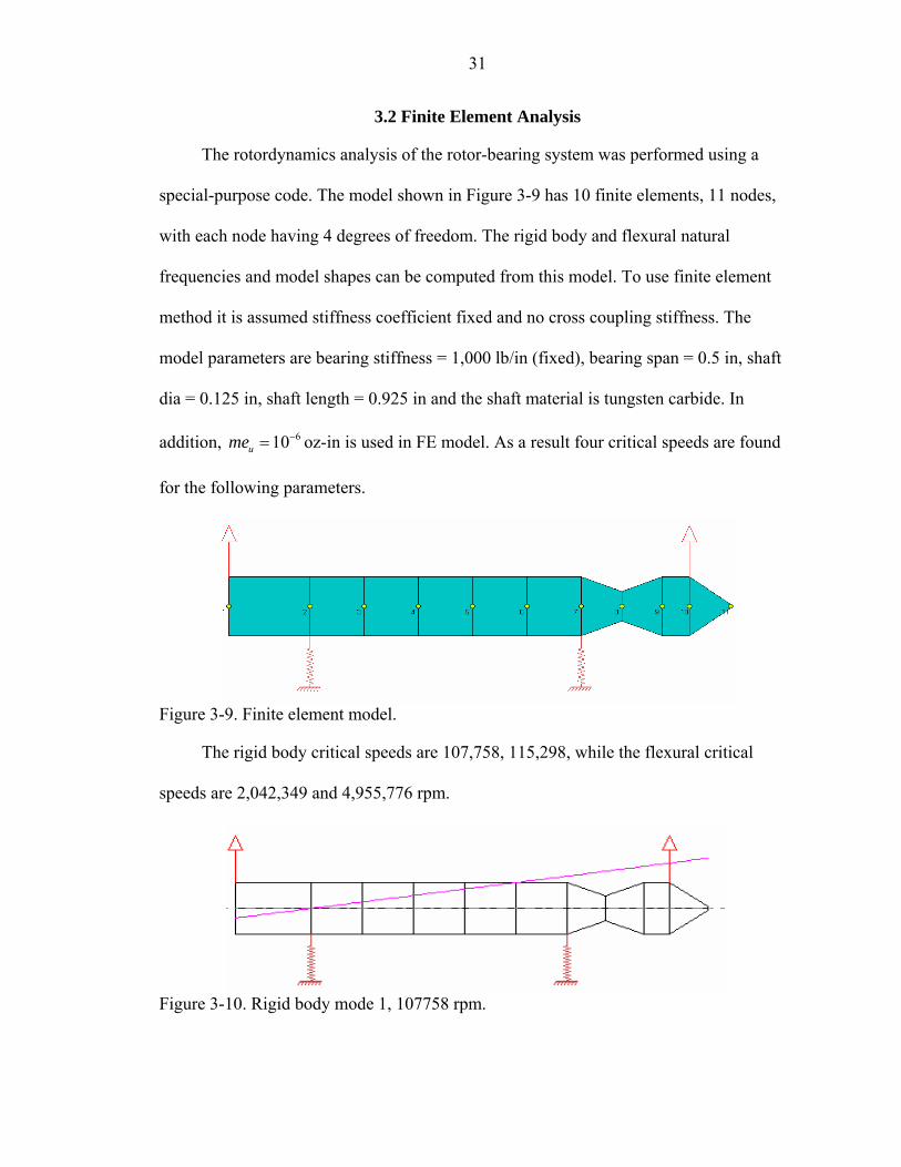
3.2 Finite Element Analysis
The rotordynamics analysis of the rotor-bearing system was performed using a
special-purpose code. The model shown in Figure 3-9 has 10 finite elements, 11 nodes,
with each node having 4 degrees of freedom. The rigid body and flexural natural
frequencies and model shapes can be computed from this model. To use finite element
method it is assumed stiffness coefficient fixed and no cross coupling stiffness. The
model parameters are bearing stiffness = 1,000 lb/in (fixed), bearing span = 0.5 in, shaft
dia = 0.125 in, shaft length = 0.925 in and the shaft material is tungsten carbide. In
addition, 610ume −= oz-in is used in FE model. As a result four critical speeds are found
for the following parameters.
Figure 3-9. Finite element model.
The rigid body critical speeds are 107,758, 115,298, while the flexural critical
speeds are 2,042,349 and 4,955,776 rpm.
Figure 3-10. Rigid body mode 1, 107758 rpm.

32
A.
B.
Figure 3-11. Rotor analysis at 115298 rpm. A) Rigid body mode 2, B) Potential energy distribution.
A.
Figure 3-12. Rotor analysis at 2,042,349 rpm. A) Flexural mode 1, B) potential energy distribution.

33
B.
Figure 3-15. Continued
Figure 3-13. Flexural mode 2, 4,955,776 rpm.
Figure 3-14. Critical speed map.

34
The critical speed map in Figure 3-14 shows that the flexural modes are unaffected
by bearing stiffness, while the two rigid body modes increase with bearing stiffness.
There are three critical points on the tool such as; two bearing positions and tool
tip. As a result the following analysis are found for these positions.
A.
B.
Figure 3-15. 1st bearing. A) and B) Unbalance response, C) Amplitude and phase lag, D) Nyquist plot for displacement.

35
C.
D.
Figure 3-15. Continued

36
A.
B.
Figure 3-16. 2nd bearing. A) and B) Unbalance response, C) Amplitude and phase lag, D) Nyquist plot for displacement.

37
C.
D.
Figure 3-16. Continued
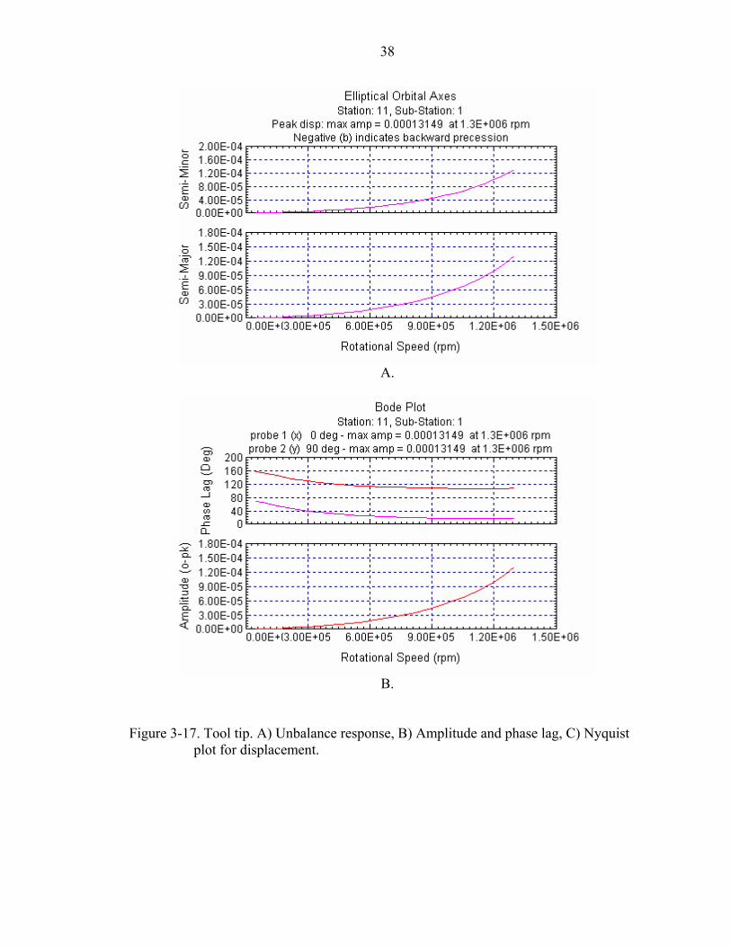
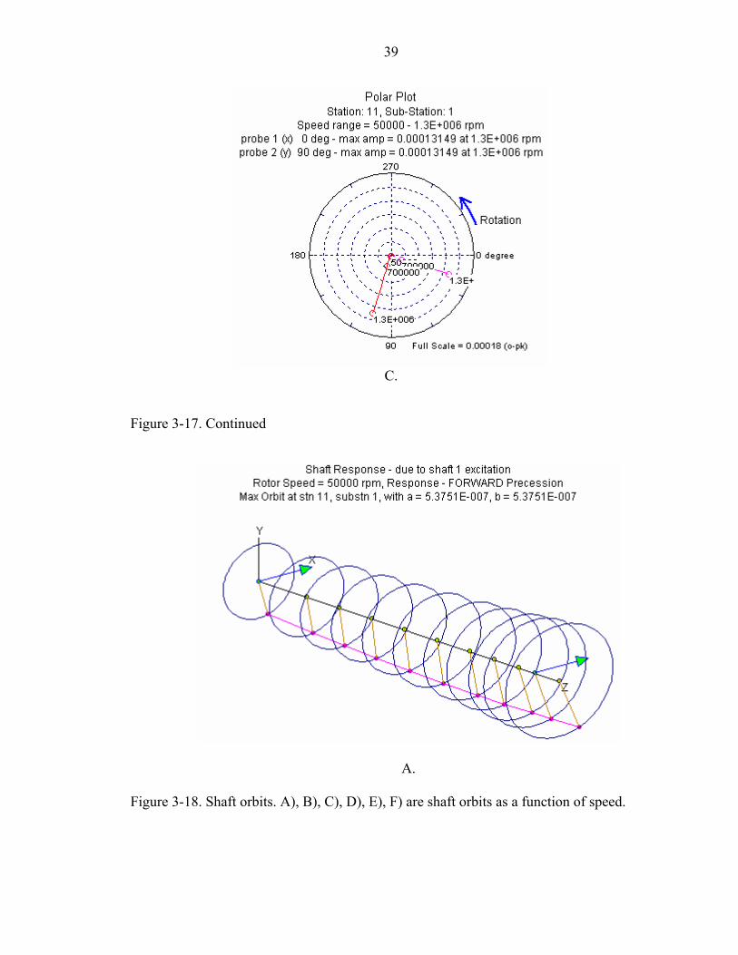
38
A.
B.
Figure 3-17. Tool tip. A) Unbalance response, B) Amplitude and phase lag, C) Nyquist plot for displacement.
39
C.
Figure 3-17. Continued
A.
Figure 3-18. Shaft orbits. A), B), C), D), E), F) are shaft orbits as a function of speed.

40
B.
C.
Figure 3-18. Continued

41
D.
E.
Figure 3-18. Continued
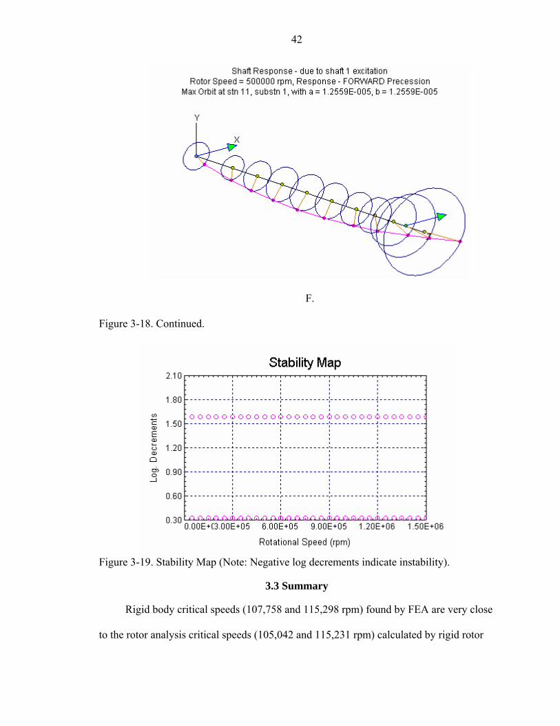
42
F.
Figure 3-18. Continued.
Figure 3-19. Stability Map (Note: Negative log decrements indicate instability).
3.3 Summary
Rigid body critical speeds (107,758 and 115,298 rpm) found by FEA are very close
to the rotor analysis critical speeds (105,042 and 115,231 rpm) calculated by rigid rotor

43
analysis. The difference occurs, because in FEA analysis cross coupling stiffness terms
and damping terms are eliminated and stiffness doesn’t change with rotor speed.
For rigid rotor analysis eccentricity ratio is calculated є=0.01, which can be
questionable to get this value in practice, and it leads 81.22 10m eu−× = ⋅ oz-in. So
unbalance response analysis is performed again with є=0.1. Figure 3-20 shows that even
with this eccentricity ratio sub micrometer runout has been obtained for a given stiffness
and damping parameters.
Orbit Amplitude
-1.00E-050.00E+001.00E-052.00E-053.00E-054.00E-055.00E-056.00E-057.00E-058.00E-059.00E-05
0 100000 200000 300000 400000 500000 600000 700000 800000Rotor speed (rpm)
Am
plitu
de (i
nch)
brg#1&2 tool tip
Figure 3-20. Orbit amplitude at 1st, 2nd bearing and tool tip, є=0.1.
Both rigid rotor analysis (see appendix B) and FEA (see figure 3-19) shows system
is stable.

44
CHAPTER 4 EXPERIMENTAL IDENTIFICATION OF BEARING PARAMETERS
In order to ensure proper operation, the vibration phenomena, which the rotors
supported by fluid film bearings are especially subject to, has to be properly predicted.
Knowledge of dynamic coefficients, stiffness and damping of a bearing prior to its
installation and operation can be highly influential in the operation costs of the final
machine. Both an analytical and experimental approach can be employed to study the
dynamic behavior of bearings. Numerical techniques and computer-based simulation are
usually used to perform analytical studies. The current research has used XlTiltPad
program to identify bearing parameters.
The test set up aims at analyzing dynamic behavior of a tilted pad air bearing,
which will be used in this research, and comparing the experimental results with
analytical results. For the time being, experiments used a commercial air bearing as the
tilted pad air bearing is in the process of being designed and for the initial studies; a
flexure-supported ball bearing (see figure 4-1) is being used. Due to the difficulties found
in exciting the rotor-bearing system and in the measurement of force and displacement
data, experimental testing on fluid film bearings is known to be complex. The bearing
parameters can be identified experimentally by six different methods as mentioned
before. Since the research deals with a micro spindle supported by a small air bearing, the
test setup will be also small making it extremely hard to use loading in order to excite the
system. As a result, the viable way is using unbalance mass method.

45
Figure 4-1. Flexure supported ball bearing: 1) Flexure, 2) Ball bearing.
4.1 Method of Measurement
The principle of operation of the test rig is rather simple: The bearing to be tested is
placed on a chassis (see figure 4-2), which serves to support displacement probes and is
mounted on dynamometer (load cell), used for measuring forces. A shaft is placed inside
the bearing and one side of shaft is mounted to the high-speed spindle. Figure 4-3 shows
a schematic of the test rig.
Z
Y
displacementprobe
load sensor
Figure 4-2. A chassis.

46
Load cell
spindle
displacementprobe
test bearing
rotor
Chasis
disk
Figure 4-3. Schematic of the test rig.
The rotating part of the test bearing has been given an intentional eccentricity at the
test bearing location. When the shaft rotates, the eccentricity generates an orbital pattern
synchronous with shaft speed.
Since the shaft is driven with a synchronous harmonic load, the resulting shaft
motion will, in general, be elliptic. Therefore, relative displacements describing ellipse as
a function of time is in following form:
( ) (cos ) (sin )y t a t b tω ω= + (4-1)
( ) (cos ) (sin )z t g t h tω ω= + (4-2)
Following equations will be used in equation of motion:
( ) (sin ) (cos )y t a t b tω ω ω ω= − +& (4-1a)
( ) (sin ) (cos )z t g t h tω ω ω ω= − +& (4-2a)

47
The four coefficients a, b, g and h are termed Fourier coefficients, and ω is the
tester speed in radians per second. They are obtained from the synchronous components
of complex frequency spectrums computed for the y and z displacements.
The air bearing will respond with reaction forces which will be read by dyno to the
off centered rotor movement. The same procedure applied to the load data which load
cells read and following equations are derived:
( ) (cos ) (sin )yF t m t n tω ω= + (4-3)
( ) (cos ) (sin )zF t p t q tω ω= + (4-4)
Equation of motion is the following:
yy yz yy yz yy yzy
zy zz zy zz zy zzz
K K C C M MF y y yK K C C M MF z z z
⎛ ⎞ ⎛ ⎞ ⎛ ⎞⎛ ⎞ ⎛ ⎞ ⎛ ⎞ ⎛ ⎞= + +⎜ ⎟ ⎜ ⎟ ⎜ ⎟⎜ ⎟ ⎜ ⎟ ⎜ ⎟ ⎜ ⎟
⎝ ⎠ ⎝ ⎠ ⎝ ⎠⎝ ⎠ ⎝ ⎠ ⎝ ⎠ ⎝ ⎠
& &&
& && (4-5)
Inertia term can be neglected in equation, because shaft relative displacement is so
small that inertia force will not contribute a lot for air film force. So new equation is the
following:
yy yz yy yzy
zy zz zy zzz
K K C CF y yK K C CF z z
⎛ ⎞ ⎛ ⎞⎛ ⎞ ⎛ ⎞ ⎛ ⎞= +⎜ ⎟ ⎜ ⎟⎜ ⎟ ⎜ ⎟ ⎜ ⎟
⎝ ⎠ ⎝ ⎠⎝ ⎠ ⎝ ⎠ ⎝ ⎠
&
& (4-6)
After substituting (4-1), (4-2), (4-1a), (4-2a), (4-3) and (4-4) into (4-6), the
following equation is obtained:
0 0 0 00 0 0 0
0 0 0 00 0 0 0
yy
yz
yy
yz
zy
zz
zy
zz
CCKb h a g mKa g b h nCb h a g pCa g b h qKK
ω ωω ω
ω ωω ω
⎧ ⎫⎪ ⎪⎪ ⎪⎪ ⎪⎛ ⎞ ⎧ ⎫⎪ ⎪⎜ ⎟ ⎪ ⎪− − ⎪ ⎪ ⎪ ⎪⎜ ⎟ =⎨ ⎬ ⎨ ⎬⎜ ⎟ ⎪ ⎪ ⎪ ⎪⎜ ⎟ ⎪ ⎪ ⎪ ⎪− −⎝ ⎠ ⎩ ⎭⎪ ⎪⎪ ⎪⎪ ⎪⎩ ⎭
(4-7)

48
Since all these bearing parameters are functions of speed, it is necessary that the
speeds span as wide a range as possible to give the best definition of the coefficients [16].
There is an example how to use equation (4-7) in Appendix D.
4.2 Design Process
The test rig was designed and developed relying on an existing dynamometer, as
seen in Figure 4-4. Detailed information about dynamometer is presented in Appendix E.
In order to facilitate a better understanding of the setup, it was divided in to four parts
that is the dyno; a main chassis (see Figure 4-5), which serves to mount displacement
probes in order to measure shaft displacement and to mount the test bearing; a shaft; and
a spindle, which is an electric driven motor and rotates at 50000 rpm (max.).
Figure 4-4. Test Setup: 1) Base, 2) Dyno, 3) Chassis, 4) Test bearing, 5) Shaft, 6) Spindle

49
Figure 4-5. Main Chassis: 1) Stator, 2) Displacement Probe, 3) Test Bearing.
The shaft motion is determined by displacement probes, and results can be read on
PC by using fiber optic sensors (RC20) connected to the PC. Dyno is used to measure the
forces in x and y directions respectively, and the data is sent to the PC using a charge
amplifier. A NSK spindle drive controller adjusts the spindle speed. The complete
measurement system is illustrated in Figure 4-6.
Figure 4-6. Measurment system

50
CHAPTER 5 CONCLUSION AND RECOMMENDATIONS
The current research provides initial results for the development of a
comprehensive rotordynamics analysis to describe high-speed micro spindle vibrations.
Results demonstrate that the air bearing characteristics and spindle residual unbalance
levels dictate the critical speed placement, unbalance response, and the ability to limit the
tool tip runout to sub-micrometer levels.
Results demonstrate that the 1/8th inch tungsten carbide micro spindle with the
integrally machined air turbine at one end and the end mill cutter at the other end can
indeed operate with sub-micrometer runout at the tool tip for spindle speeds up to 1
million rpm. Air bearing stiffness used is about 2000 lb/in. Spindle residual unbalance
level assumed is 10-6 oz-in (me=. 000001 oz-in). Residual unbalance two to three times
this level will also be adequate with higher bearing stiffness. Turbine engine shafts
weighing 100 lbs or greater are routinely balanced to 0.1 oz-in. Considering that the end
mill cutter weighs about 0.07 lb, the recommended unbalance limits can be achieved in
practice.
Next step in this research is experimental analysis, which was undertaken to
understand behavior of the air bearing. Since the air bearing is yet to be fabricated, a
simple test rig has been built to test the spindle mounted on ball bearings with a flexure
support. The x-y displacements at the bearings, as a function of speed, are being used to
evaluate the support stiffness characteristics. Our goals are to demonstrate the feasibility
of the proposed parameter estimation scheme to evaluate support stiffness.

51
APPENDIX A CHRONOLOGICAL LIST OF PAPERS ON THE EXPERIMENTAL DYNAMIC
PARAMETER IDENTIFICATION OF BEARINGS

52

53

54
* The following abbreviations are used in the table: AGS, annular gas seal; ANS, annular
seal; ALS, annular liquid seal; BS, brush seals; DS, damper seals; ER, electrorheological
fluid; FAB, foil air; FTB, foil thrust; GDS, gas damper seal; GJ, gas journal; GS, gas
seal; HCS, honeycombed seal; HDJ, hydrodynamic journal; HSJ, hydrostatic journal;
HYJ, hybrid journal; LGS, long gas seal; LS, long seal; MB, magnetic; MD, metal mess
bearing damper; PLS, plain liquid seal; RB, recirculating ball; RE, rolling element; SPR,
springs; SQF, squeeze film; TPJ, tilting pad journal; TR, tapered roller.

APPENDIX B GENERAL RIGID ROTOR SOLUTION 1

56
Input Rigid Rotor Parameters
lbf-sec^2/in a1 0.6:= inch m
0.09748386
:=
a2 0.6−:=lbf-sec^2-in Ip
0.001616386
:= eu 0.000002:= unbalance eccentricity, in
lbf-sec^2-in Id
1.889 10 5−⋅
386:=
euθπ
4:=
η eu cos euθ( )⋅:= ζ eu sin euθ( )⋅:= Ω 52359.9:= rad
sec
η 1.41421 10 6−×= ζ 1.41421 10 6−
×=
Kyy1 2055.3:= Kyy2 2055.3:= lbf/in Cyy1 0.014:= Cyy2 0.014:= lbf-sec/in
Kyz1 147.6:= Kyz2 147.6:= Cyz1 0.0071−:= Cyz2 0.0071−:= Kzy1 91.36−:= Kzy2 91.36−:= Czy1 0.005:= Czy2 0.005:= Kzz1 1713.13:= Kzz2 1713.13:= Czz1 0.035:= Czz2 0.035:=

57
A
Kyy1 Kyy2+ Ω( )2 m⋅−
Kzy1 Kzy2+
a1 Kzy1⋅ a2 Kzy2⋅+
a1 Kyy1⋅ a2 Kyy2⋅+( )−
Ω− Cyy1 Cyy2+( )⋅
Ω− Czy1 Czy2+( )⋅
Ω− a1 Czy1⋅ a2 Czy2⋅+( )⋅
Ω a1 Cyy1⋅ a2 Cyy2⋅+( )⋅
Kyz1 Kyz2+
Kzz1 Kzz2+ Ω( )2 m⋅−
a1 Kzz1⋅ a2 Kzz2⋅+
a1 Kyz1⋅ a2 Kyz2⋅+( )−
Ω− Cyz1 Cyz2+( )⋅
Ω− Czz1 Czz2+( )⋅
Ω− a1 Czz1⋅ a2 Czz2⋅+( )⋅
Ω a1 Cyz1⋅ a2 Cyz2⋅+( )⋅
a1 Kyz1⋅ a2 Kyz2⋅+
a1 Kzz1⋅ a2 Kzz2⋅+
a12 Kyy1⋅ a22 Kzz2⋅+ Ω( )2 Id⋅−
a12 Kyz1⋅ a22 Kyz2⋅+( )−
Ω− a1 Cyz1⋅ a2 Cyz2⋅+( )⋅
Ω− a1 Czz1⋅ a2 Czz2⋅+( )⋅
Ω− a12 Cyy1⋅ a22 Czz2⋅+( )⋅
Ω a12 Cyz1⋅ a22 Cyz2⋅+( )⋅ Ω( )2 Ip⋅+
a1 Kyy1⋅ a2 Kyy2⋅+( )−
a1 Kzy1⋅ a2 Kzy2⋅+( )−
a12 Kzy1⋅ a22 Kzy2⋅+( )−
a12 Kzz1⋅ a22 Kzz2⋅+ Ω( )2 Id⋅−
Ω a1 Cyy1⋅ a2 Cyy2⋅+( )⋅
Ω a1 Czy1⋅ a2 Czy2⋅+( )⋅
Ω a12 Czy1⋅ a22 Czy2⋅+( )⋅ Ω( )2 Ip⋅−
Ω− a12 Czz1⋅ a22 Czz2⋅+( )⋅
Ω Cyy1 Cyy2+( )⋅
Ω Czy1 Czy2+( )⋅
Ω a1 Czy1⋅ a2 Czy2⋅+( )⋅
Ω− a1 Cyy1⋅ a2 Cyy2⋅+( )⋅
Kyy1 Kyy2+ Ω( )2 m⋅−
Kzy1 Kzy2+
a1 Kzy1⋅ a2 Kzy2⋅+
a1 Kyy1⋅ a2 Kyy2⋅+( )−
Ω Cyz1 Cyz2+( )⋅
Ω Czz1 Czz2+( )⋅
Ω a1 Czz1⋅ a2 Czz2⋅+( )⋅
Ω− a1 Cyz1⋅ a2 Cyz2⋅+( )⋅
Kyz1 Kyz2+
Kzz1 Kzz2+ Ω( )2 m⋅−
a1 Kzz1⋅ a2 Kzz2⋅+
a1 Kyz1⋅ a2 Kyz2⋅+( )−
Ω a1 Cyz1⋅ a2 Cyz2⋅+( )⋅
Ω a1 Czz1⋅ a2 Czz2⋅+( )⋅
Ω a12 Cyy1⋅ a22 Czz2⋅+( )⋅
Ω− a12 Cyz1⋅ a22 Cyz2⋅+( )⋅ Ω( )2 Ip⋅−
a1 Kyz1⋅ a2 Kyz2⋅+
a1 Kzz1⋅ a2 Kzz2⋅+
a12 Kzz1⋅ a22 Kzz2⋅+ Ω( )2 Id⋅−
a12 Kyz1⋅ a22 Kyz2⋅+( )−
Ω− a1 Cyy1⋅ a2 Cyy2⋅+( )⋅
Ω− a1 Czy1⋅ a2 Czy2⋅+( )⋅
Ω− a12 Czy1⋅ a22 Czy2⋅+( )⋅ Ω( )2 Ip⋅+
Ω a12 Czz1⋅ a22 Czz2⋅+( )⋅
a1 Kyy1⋅ a2 Kyy2⋅+( )−
a1 Kzy1⋅ a2 Kzy2⋅+( )−
a12 Kzy1⋅ a22 Kzy2⋅+( )−
a12 Kyy1⋅ a22 Kyy2⋅+ Ω( )2 Id⋅−
⎡⎢⎢⎢⎢⎢⎢⎢⎢⎢⎢⎢⎢⎢⎢⎣
⎤⎥⎥⎥⎥⎥⎥⎥⎥⎥⎥⎥⎥⎥⎥⎦
:=
(RHS unbalance forcing terms) RHS m Ω( )2⋅
η
ζ
0
0
ζ−
η
0
0
⎛⎜⎜⎜⎜⎜⎜⎜⎜⎜⎝
⎞
⎟⎟⎟⎟⎟⎟⎟
⎠
⋅:= RHS
0.09791
0.09791
0
0
0.09791−
0.09791
0
0
⎛⎜⎜⎜⎜⎜⎜⎜⎜⎜⎝
⎞
⎟⎟⎟⎟⎟⎟⎟
⎠
=

58
A
67306.42171−
18.944
0
0
3141.594−
52.3599−
0
0
25.2
66987.02171−
0
0
429.35118
3508.1133−
0
0
0
0
617.62206
9.072−
0
0
1196.94731−
11323.04899
0
0
6.81984−
675.11406
0
0
11458.76585−
1262.92079−
3141.594
52.3599
0
0
67306.42171−
18.944
0
0
429.35118−
3508.1133
0
0
25.2
66987.02171−
0
0
0
0
1196.94731
11323.04899−
0
0
675.11406
9.072−
0
0
11458.76585
1262.92079
0
0
6.81984−
560.13006
⎛⎜⎜⎜⎜⎜⎜⎜⎜⎜⎝
⎞
⎟⎟⎟⎟⎟⎟⎟
⎠
=
q A 1− RHS⋅:= Bearing Orbits
Bearing #1
V1c q0 a1 q3⋅−:= W1c q1 a1 q2⋅+:=
V1s q4 a1 q7⋅−:= W1s q5 a1 q6⋅+:=
q
1.37609− 10 6−×
1.53315− 10 6−×
0
0
1.50867 10 6−×
1.37988− 10 6−×
0
0
⎛⎜⎜⎜⎜⎜⎜⎜⎜⎜⎜⎜⎝
⎞
⎟⎟⎟⎟⎟⎟⎟⎟⎟
⎠
= Bearing #2
V2c q0 a2 q3⋅−:= W2c q1 a2 q2⋅+:=
V2s q4 a2 q7⋅−:= W2s q5 a2 q6⋅+:=

59
2 .10 6 1 .10 6 0 1 .10 6 2 .10 6
2 .10 6
1 .10 6
1 .10 6
2 .10 6
shaft displacement in y direction
shaf
t dis
plac
emen
t in
z di
rect
ion
2.06256 10 6−×
2.06256− 10 6−×
W2 t( )
2.04177 10 6−×2.04177− 10 6−× V2 t( )
PLOT BEARING ORBITS
T2 π⋅
Ω:= T 0.00012=
t 0T
200, T..:=
Bearing #1 Bearing #2
V1 t( ) V1c cos Ω t⋅( )⋅ V1s sin Ω t⋅( )⋅+:= V2 t( ) V2c cos Ω t⋅( )⋅ V2s sin Ω t⋅( )⋅+:=
W1 t( ) W1c cos Ω t⋅( )⋅ W1s sin Ω t⋅( )⋅+:= W2 t( ) W2c cos Ω t⋅( )⋅ W2s sin Ω t⋅( )⋅+:=
2 .10 6 1 .10 6 0 1 .10 6 2 .10 6
2 .10 6
1 .10 6
1 .10 6
2 .10 6
shaft displacement in y direction
shaf
t dis
plac
emen
t in
z di
rect
ion
W1 t( )
V1 t( )

60
Work done per cycle at the bearings
Bearing #1
Kd1Kyz1 Kzy1+
2:= Cm1
Cyy1 Czz1+
2:=
WK1Cir 2 π⋅ Kd1⋅ V1c W1s⋅ V1s W1c⋅−( )⋅:= Work done by Circulation Force at Bearing #1
WK1Diss π− Ω⋅ Cyy1 V1c2 W1s2+( )⋅ 2 Cm1⋅ V1c W1c⋅ V1s W1s⋅+( )⋅+ Czz1 W1c2 W1s2
+( )⋅+⎡⎣ ⎤⎦⋅:= Work done by dissipation forces
WK1Total WK1Cir WK1Diss+:= Total work done at the bearing #1
Bearing #2
Kd2Kyz2 Kzy2+
2:= Cm2
Cyy2 Czz2+
2:=
WK2Cir 2 π⋅ Kd2⋅ V2c W2s⋅ V2s W2c⋅−( )⋅:= Work done by Circulation Force at Bearing #2
WK2Diss π− Ω⋅ Cyy2 V2c2 W2s2+( )⋅ 2 Cm2⋅ V2c W2c⋅ V2s W2s⋅+( )⋅+ Czz2 W2c2 W2s2
+( )⋅+⎡⎣ ⎤⎦⋅:= Work done by dissipation forces
WK2Total WK2Cir WK2Diss+:= Total work done at the bearing #2

61
Bearing #1 Bearing #2
WK1Cir 4.13906 10 11−×= WK2Cir 4.13906 10 11−
×=
WK1Diss 4.24666− 10 8−×= WK2Diss 4.24666− 10 8−
×=
WK1Total 4.24253− 10 8−×= WK2Total 4.24253− 10 8−
×=
NOTE: Total work done at each bearing/cycle must be negative(subtracting energy from rotor), for stable operation

APPENDIX C GENERAL RIGID ROTOR SOLUTION 2

63
Bearing parameters found by using XLTiltPadHGB:
Input Rigid Rotor Parameters
lbf-sec^2/in a1 0.6:= inch m
0.09748386
:=
a2 0.6−:=lbf-sec^2-in Ip
0.001616386
:= eu 0.000002:= unbalance eccentricity, in
lbf-sec^2-in Id
1.889 10 5−⋅
386:=
euθπ
4:=
η eu cos euθ( )⋅:= ζ eu sin euθ( )⋅:= Ω 52359.9:= rad
sec
η 1.41421 10 6−×= ζ 1.41421 10 6−
×=
Kyy1 2055.3:= Kyy2 2055.3:= lbf/in Cyy1 0.014:= Cyy2 0.014:= lbf-sec/in
Kyz1 147.6:= Kyz2 147.6:= Cyz1 0.0071−:= Cyz2 0.0071−:= Kzy1 91.36−:= Kzy2 91.36−:= Czy1 0.005:= Czy2 0.005:=
Kzz1 1713.13:= Kzz2 1713.13:= Czz1 0.035:= Czz2 0.035:=

64
A
Kyy1 Kyy2+ Ω( )2 m⋅−
Kzy1 Kzy2+
a1Kzy1⋅ a2Kzy2⋅+
a1Kyy1⋅ a2Kyy2⋅+( )−
Ω− Cyy1 Cyy2+( )⋅
Ω− Czy1 Czy2+( )⋅
Ω− a1Czy1⋅ a2Czy2⋅+( )⋅
Ω a1Cyy1⋅ a2Cyy2⋅+( )⋅
Kyz1 Kyz2+
Kzz1 Kzz2+ Ω( )2 m⋅−
a1Kzz1⋅ a2Kzz2⋅+
a1Kyz1⋅ a2Kyz2⋅+( )−
Ω− Cyz1 Cyz2+( )⋅
Ω− Czz1 Czz2+( )⋅
Ω− a1Czz1⋅ a2Czz2⋅+( )⋅
Ω a1Cyz1⋅ a2Cyz2⋅+( )⋅
a1Kyz1⋅ a2Kyz2⋅+
a1Kzz1⋅ a2Kzz2⋅+
a12 Kyy1⋅ a22 Kzz2⋅+ Ω( )2 Id⋅−
a12 Kyz1⋅ a22 Kyz2⋅+( )−
Ω− a1Cyz1⋅ a2Cyz2⋅+( )⋅
Ω− a1Czz1⋅ a2Czz2⋅+( )⋅
Ω− a12 Cyy1⋅ a22 Czz2⋅+( )⋅
Ω a12 Cyz1⋅ a22 Cyz2⋅+( )⋅ Ω( )2 Ip⋅+
a1Kyy1⋅ a2Kyy2⋅+( )−
a1Kzy1⋅ a2Kzy2⋅+( )−
a12 Kzy1⋅ a22 Kzy2⋅+( )−
a12 Kzz1⋅ a22 Kzz2⋅+ Ω( )2 Id⋅−
Ω a1Cyy1⋅ a2Cyy2⋅+( )⋅
Ω a1Czy1⋅ a2Czy2⋅+( )⋅
Ω a12 Czy1⋅ a22 Czy2⋅+( )⋅ Ω( )2 Ip⋅−
Ω− a12 Czz1⋅ a22 Czz2⋅+( )⋅
Ω Cyy1 Cyy2+( )⋅
Ω Czy1 Czy2+( )⋅
Ω a1Czy1⋅ a2Czy2⋅+( )⋅
Ω− a1Cyy1⋅ a2Cyy2⋅+( )⋅
Kyy1 Kyy2+ Ω( )2 m⋅−
Kzy1 Kzy2+
a1Kzy1⋅ a2Kzy2⋅+
a1Kyy1⋅ a2Kyy2⋅+( )−
Ω Cyz1 Cyz2+( )⋅
Ω Czz1 Czz2+( )⋅
Ω a1Czz1⋅ a2Czz2⋅+( )⋅
Ω− a1Cyz1⋅ a2Cyz2⋅+( )⋅
Kyz1 Kyz2+
Kzz1 Kzz2+ Ω( )2 m⋅−
a1Kzz1⋅ a2Kzz2⋅+
a1Kyz1⋅ a2Kyz2⋅+( )−
Ω a1Cyz1⋅ a2Cyz2⋅+( )⋅
Ω a1Czz1⋅ a2Czz2⋅+( )⋅
Ω a12 Cyy1⋅ a22 Czz2⋅+( )⋅
Ω− a12 Cyz1⋅ a22 Cyz2⋅+( )⋅ Ω( )2 Ip⋅−
a1Kyz1⋅ a2Kyz2⋅+
a1Kzz1⋅ a2Kzz2⋅+
a12 Kzz1⋅ a22 Kzz2⋅+ Ω( )2 Id⋅−
a12 Kyz1⋅ a22 Kyz2⋅+( )−
Ω− a1Cyy1⋅ a2Cyy2⋅+( )⋅
Ω− a1Czy1⋅ a2Czy2⋅+( )⋅
Ω− a12 Czy1⋅ a22 Czy2⋅+( )⋅ Ω( )2 Ip⋅+
Ω a12 Czz1⋅ a22 Czz2⋅+( )⋅
a1Kyy1⋅ a2Kyy2⋅+( )−
a1Kzy1⋅ a2Kzy2⋅+( )−
a12 Kzy1⋅ a22 Kzy2⋅+( )−
a12 Kyy1⋅ a22 Kyy2⋅+ Ω( )2 Id⋅−
⎡⎢⎢⎢⎢⎢⎢⎢⎢⎢⎢⎢⎢⎢⎢⎣
⎤⎥⎥⎥⎥⎥⎥⎥⎥⎥⎥⎥⎥⎥⎥⎦
:=
(RHS unbalance forcing terms) RHS m Ω( )2⋅
η
ζ
0
0
ζ−
η
0
0
⎛⎜⎜⎜⎜⎜⎜⎜⎜⎜⎝
⎞
⎟⎟⎟⎟⎟⎟⎟
⎠
⋅:= RHS
0.09791
0.09791
0
0
0.09791−
0.09791
0
0
⎛⎜⎜⎜⎜⎜⎜⎜⎜⎜⎝
⎞
⎟⎟⎟⎟⎟⎟⎟
⎠
=

65
A
65124.42171−
182.72−
0
0
1466.0772−
523.599−
0
0
295.2
65808.76171−
0
0
743.51058
3665.193−
0
0
0
0
1222.46886
106.272−
0
0
923.62864−
11209.95161
0
0
65.7792
1099.28766
0
0
11289.11978−
1319.46948−
1466.0772
523.599
0
0
65124.42171−
182.72−
0
0
743.51058−
3665.193
0
0
295.2
65808.76171−
0
0
0
0
923.62864
11209.95161−
0
0
1099.28766
106.272−
0
0
11289.11978
1319.46948
0
0
65.7792
1345.65006
⎛⎜⎜⎜⎜⎜⎜⎜⎜⎜⎝
⎞
⎟⎟⎟⎟⎟⎟⎟
⎠
=
q A 1− RHS⋅:= Bearing Orbits
Bearing #1
V1c q0 a1 q3⋅−:= W1c q1 a1 q2⋅+:=
V1s q4 a1 q7⋅−:= W1s q5 a1 q6⋅+:=
q
1.46054− 10 6−×
1.5494− 10 6−×
0
0
1.51235 10 6−×
1.39413− 10 6−×
0
0
⎛⎜⎜⎜⎜⎜⎜⎜⎜⎜⎜⎜⎝
⎞
⎟⎟⎟⎟⎟⎟⎟⎟⎟
⎠
= Bearing #2
V2c q0 a2 q3⋅−:= W2c q1 a2 q2⋅+:=
V2s q4 a2 q7⋅−:= W2s q5 a2 q6⋅+:=

66
2 .10 6 1 .10 6 0 1 .10 6 2 .10 6
2 .10 6
1 .10 6
1 .10 6
2 .10 6
shaft displacement in y direction
shaf
t dis
plac
emen
t in
z di
rect
ion
W1 t( )
V1 t( )
PLOT BEARING ORBITS
T2 π⋅
Ω:= T 0.00012=
t 0T
200, T..:=
Bearing #1 Bearing #2
V1 t( ) V1c cos Ω t⋅( )⋅ V1s sin Ω t⋅( )⋅+:= V2 t( ) V2c cos Ω t⋅( )⋅ V2s sin Ω t⋅( )⋅+:=
W1 t( ) W1c cos Ω t⋅( )⋅ W1s sin Ω t⋅( )⋅+:= W2 t( ) W2c cos Ω t⋅( )⋅ W2s sin Ω t⋅( )⋅+:=
2 .10 6 1 .10 6 0 1 .10 6 2 .10 6
2 .10 6
1 .10 6
1 .10 6
2 .10 6
shaft displacement in y direction
shaf
t dis
plac
emen
t in
z di
rect
ion
W2 t( )
V2 t( )

67
Work done per cycle at the bearings
Bearing #1
Kd1Kyz1 Kzy1+
2:= Cm1
Cyy1 Czz1+
2:=
WK1Cir 2 π⋅ Kd1⋅ V1c W1s⋅ V1s W1c⋅−( )⋅:= Work done by Circulation Force at Bearing #1
WK1Diss π− Ω⋅ Cyy1 V1c2 W1s2+( )⋅ 2 Cm1⋅ V1c W1c⋅ V1s W1s⋅+( )⋅+ Czz1 W1c2 W1s2
+( )⋅+⎡⎣ ⎤⎦⋅:= Work done by dissipation forces
WK1Total WK1Cir WK1Diss+:= Total work done at the bearing #1
Bearing #2
Kd2Kyz2 Kzy2+
2:= Cm2
Cyy2 Czz2+
2:=
WK2Cir 2 π⋅ Kd2⋅ V2c W2s⋅ V2s W2c⋅−( )⋅:= Work done by Circulation Force at Bearing #2
WK2Diss π− Ω⋅ Cyy2 V2c2 W2s2+( )⋅ 2 Cm2⋅ V2c W2c⋅ V2s W2s⋅+( )⋅+ Czz2 W2c2 W2s2
+( )⋅+⎡⎣ ⎤⎦⋅:= Work done by dissipation forces
WK2Total WK2Cir WK2Diss+:= Total work done at the bearing #2

68
Bearing #1 Bearing #2
WK1Cir 7.73768 10 10−×= WK2Cir 7.73768 10 10−
×=
WK1Diss 3.56451− 10 8−×= WK2Diss 3.56451− 10 8−
×=
WK1Total 3.48713− 10 8−×= WK2Total 3.48713− 10 8−
×=
NOTE: Total work done at each bearing/cycle must be negative (subtracting energy from rotor), for stable operation

69
APPENDIX D EXAMPLE OF FINDING BEARING PARAMETERS
Let's choose two different speed, and different displacement components for each speed.
So by assuming all variables, forces can be find by using equation of motion (4-6),
where
Fy(θ)=m*cos(θ)+n*sin(θ) and Fz(θ)=p*cos(θ)+q*sin(θ).
Ω 2 104⋅:= rad/sec a 0.03:= b 0.01:= g 0.02:= h 0.03:=
Ω1 2.1 104⋅:=
a1 0.036:= b1 0.016:= g1 0.026:= h1 0.036:=
θ 0 2π
100⋅, 2 π⋅..:= where θ=Ωt
z1 θ( ) g1 cos θ( )⋅ h1 sin θ( )⋅+:=
0.05 0 0.050.05
0
0.05
z θ( )
y θ( )
z θ( ) g cos θ( )⋅ h sin θ( )⋅+:=
y θ( ) a cos θ( )⋅ b sin θ( )⋅+:= y1 θ( ) a1 cos θ( )⋅ b1 sin θ( )⋅+:=
0.05 0 0.050.05
0
0.05
z1 θ( )
y1 θ( )
Let Kyy 1000:= Kzy 500−:= lbf/in Cyy 15:= Czy 4−:= lbf-sec/in Kyz 500:= Kzz 900:= Cyz 4:= Czz 15:=

70
Now by using force and displacement components, lets find stiffness and damping
coefficients.
For each speed, there are set of four equations, expressed above. Thus for two
different speeds, following expression is obtained:
As it can be seen, stiffness and damping coefficients are the same values as assumed.
m a Kyy⋅ g Kyz⋅+ b Ω⋅ Cyy⋅+ h Ω⋅ Cyz⋅+:= m1 a1 Kyy⋅ g1 Kyz⋅+ b1 Ω1⋅ Cyy⋅+ h1 Ω1⋅ Cyz⋅+:=
n b Kyy⋅ h Kyz⋅+ a Ω⋅ Cyy⋅− g Ω⋅ Cyz⋅−:= n1 b1 Kyy⋅ h1 Kyz⋅+ a1 Ω1⋅ Cyy⋅− g1 Ω1⋅ Cyz⋅−:=
p a Kzy⋅ g Kzz⋅+ b Ω⋅ Czy⋅+ h Ω⋅ Czz⋅+:= p1 a1 Kzy⋅ g1 Kzz⋅+ b1 Ω1⋅ Czy⋅+ h1 Ω1⋅ Czz⋅+:=
q b Kzy⋅ h Kzz⋅+ a Ω⋅ Czy⋅− g Ω⋅ Czz⋅−:= q1 b1 Kzy⋅ h1 Kzz⋅+ a1 Ω1⋅ Czy⋅− g1 Ω1⋅ Czz⋅−:=
P
b Ω⋅
a− Ω⋅
0
0
h Ω⋅
g− Ω⋅
0
0
a
b
0
0
g
h
0
0
0
0
b Ω⋅
a− Ω⋅
0
0
h Ω⋅
g− Ω⋅
0
0
a
b
0
0
g
h
⎛⎜⎜⎜⎜⎝
⎞
⎟⎟
⎠
:= T
m
n
p
q
⎛⎜⎜⎜⎜⎝
⎞⎟⎟
⎠
:=
T1
m
n
p
q
m1
n1
p1
q1
⎛⎜⎜⎜⎜⎜⎜⎜⎜⎜⎝
⎞
⎟⎟⎟⎟⎟⎟⎟
⎠
:= P1
b Ω⋅
a− Ω⋅
0
0
b1 Ω1⋅
a1− Ω1⋅
0
0
h Ω⋅
g− Ω⋅
0
0
h1 Ω1⋅
g1− Ω1⋅
0
0
a
b
0
0
a1
b1
0
0
g
h
0
0
g1
h1
0
0
0
0
b Ω⋅
a− Ω⋅
0
0
b1 Ω1⋅
a1− Ω1⋅
0
0
h Ω⋅
g− Ω⋅
0
0
h1 Ω1⋅
g1− Ω1⋅
0
0
a
b
0
0
a1
b1
0
0
g
h
0
0
g1
h1
⎛⎜⎜⎜⎜⎜⎜⎜⎜⎜⎜⎝
⎞⎟⎟⎟⎟⎟⎟⎟⎟
⎠
:=
Ans P1 1− T1⋅:=
Ans
15
4
1000
500
4−
15
500−
900
⎛⎜⎜⎜⎜⎜⎜⎜⎜⎜⎝
⎞
⎟⎟⎟⎟⎟⎟⎟
⎠
=
Cyy
Cyz
Kyy
Kyz
Czy
Czz
Kzy
Kzz
⎛⎜⎜⎜⎜⎜⎜⎜⎜⎜⎝
⎞
⎟⎟⎟⎟⎟⎟⎟
⎠

71
Let's assume force data were read in error, because of noise. Forces in y direction and
forces in z direction are read in ten and four percent error, respectively.
The result shows that the stiffness and damping coefficients are changed by the
same percentage as forces. So it means noise in force affects bearing parameters at the
same percentage as in force itself.
m m 1.1⋅:= n n 1.1⋅:= p p 1.04⋅:= q q 1.04⋅:=
m1 m1 1.1⋅:= n1 n1 1.1⋅:= p1 p1 1.04⋅:= q1 q1 1.04⋅:=
P1
b Ω⋅
a− Ω⋅
0
0
b1 Ω1⋅
a1− Ω1⋅
0
0
h Ω⋅
g− Ω⋅
0
0
h1 Ω1⋅
g1− Ω1⋅
0
0
a
b
0
0
a1
b1
0
0
g
h
0
0
g1
h1
0
0
0
0
b Ω⋅
a− Ω⋅
0
0
b1 Ω1⋅
a1− Ω1⋅
0
0
h Ω⋅
g− Ω⋅
0
0
h1 Ω1⋅
g1− Ω1⋅
0
0
a
b
0
0
a1
b1
0
0
g
h
0
0
g1
h1
⎛⎜⎜⎜⎜⎜⎜⎜⎜⎜⎜⎝
⎞⎟⎟⎟⎟⎟⎟⎟⎟
⎠
:= T1
m
n
p
q
m1
n1
p1
q1
⎛⎜⎜⎜⎜⎜⎜⎜⎜⎜⎝
⎞
⎟⎟⎟⎟⎟⎟⎟
⎠
:=
Ans P1 1− T1⋅:=
Ans
16.5
4.4
1.1 103×
550
4.16−
15.6
520−
936
⎛⎜⎜⎜⎜⎜⎜⎜⎜⎜⎜⎝
⎞⎟⎟⎟⎟⎟⎟⎟⎟
⎠
=

72
APPENDIX E KISTLER DYNANOMETER

73

74
LIST OF REFERENCES
[1] Kussul, E. M., Rachkovskij, D. A., Baidyk, T. N., and Talayev, S. A., 1996, “Micromechanical engineering: A basis for the l0w-cost manufacturing for mechanical microdevices using microequipment,” Journal of Micromechanical Microengineering, vol. 6, pp. 410–425.
[2] Masuzawa, T., and Tonshoff, H. K., 1997, “Three-dimensional micromachining by machine tools,” Annals of the CIRP, vol. 46, pp. 621–628.
[3] Roy R. Craig, Jr., 1981, “Structural Dynamics,” 1st edition, pp. 430-434.
[4] Tiwari, R., Lees, A. W., and Friswell, M. I., 2004, “Identification of Dynamic Bearing Parameters: A review,” The Shock and Vibration Digest, vol. 36, pp. 99-124.
[5] Mitchell, J.R., Holmes, R., and Ballegooyen, H.V., 1965–66, “Experimental Determination of a Bearing Oil Film Stiffness,” in Proceedings of the 4th Lubrication and Wear Convention, IMechE, Vol. 180, No. 3K, 90–96.
[6] Arumugam, P., Swarnamani, S., and Prabhu, B. S., 1995, “Experimental Identification of Linearized Oil Film Coefficients of Cylindrical and Tilting Pad Bearings,” ASME Journal of Engineering for Gas Turbines and Power, Vol. 117, No. 3, 593–599.
[7] Glienicke, J., 1966–67, “Experimental Investigation of the Stiffness and Damping Coefficients of Turbine Bearings and Their Application to Instability Prediction,” Proceedings of IMechE, Vol. 181, No. 3B, 116–129.
[8] Morton, P.G., 1971, “Measurement of the Dynamic Characteristics of Large Sleeve Bearing,” ASME Journal of Lubrication Technology, Vol. 93, No.1, 143–150.
[9] Someya, T., 1976, “An Investigation into the Spring and Damping Coefficients of the Oil Film in Journal Bearing,” Transactions of the Japan Society of Mechanical Engineers, Vol. 42, No. 360, 2599–2606.
[10] Hisa, S., Matsuura, T., and Someya, T., 1980, “Experiments on the Dynamic Characteristics of Large Scale Journal Bearings,” in Proceedings of the 2nd International Conference on Vibration in Rotating Machinery, IMechE, Cambridge, UK, Paper C284, 223–230.

75
[11] Sakakida, H., Asatsu, S., and Tasaki, S., 1992, “The Static and Dynamic Characteristics of 23 Inch (584.2 mm) Diameter Journal Bearing,” in Proceedings of the 5th International Conference on Vibration in Rotating Machinery, IMechE, Bath, UK, Paper C432/057, 351–358.
[12] Hagg, A.C., and Sankey, G.O., 1956, “Some Dynamic Properties of Oil-Film Journal Bearings with Reference to the Unbalance Vibration of Rotors,” ASME Journal of Applied Mechanics, Vol. 78, No. 2, 302–305.
[13] Hagg, A.C., and Sankey, G.O., 1958, “Elastic and Damping Properties of Oil-Film Journal Bearings for Application to Unbalance Vibration Calculations,” ASME Journal of Applied Mechanics, Vol. 80, No. 1, 141–143.
[14] Stone, J.M., and Underwood, A.F., 1947, “Load-Carrying Capacity of Journal Bearing,” SAE Quarterly Transactions, Vol. 1, No. 1, 56–70.
[15] Duffin, S., and Johnson, B.T., 1966–67, “Some Experimental and Theoretical Studies of Journal Bearings for Large Turbine-Generator Sets,” Proceedings of IMechE, Vol. 181, Part 3B, 89–97.
[16] Murphy, B.T., and Wagner, M.N., 1991, “Measurement of Rotordynamic Coefficients for a Hydrostatic Radial Bearing,” ASME Journal of Tribology, Vol. 113, No. 3, 518–525.
[17] Adams, M.L., Sawicki, J.T., and Capaldi, R.J., 1992, “Experimental Determination of Hydrostatic Journal Bearing Rotordynamic Coefficients,” in Proceedings of the 5th International Conference on Vibration in Rotating Machinery, IMechE, Bath, UK, Paper C432/145, 365–374.
[18] Sawicki, J.T., Capaldi, R.J., and Adams M.L., 1997, “Experimental and Theoretical Rotordynamic Characteristics of a Hybrid Journal Bearing,” ASME Journal of Tribology, Vol. 119, No. 1, 132–142.
[19] Downham, E., and Woods, R., 1971, “The Rationale of Monitoring Vibration on Rotating Machinery in Continuously Operating Process Plant,” in ASME Vibration Conference, Paper No. 71-Vibr-96.
[20] Nordmann, R., 1975, “Identification of Stiffness and Damping Coefficients of Journal Bearings by Means of the Impact Method,” in Dynamics of Rotors: Stability and System Identification, O. Mahrenholtz, ed., Springer-Verlag, New York, 395–409.
[21] Nordmann, R., and Schöllhorn, K., 1980, “Identification of Stiffness and Damping Coefficients of Journal Bearings by Means of the Impact Method,” in Proceedings of the 2nd International Conference on Vibration in Rotating Machinery, IMechE, Cambridge, UK, Paper C285, 231–238.

76
[22] Zhang, Y.Y., Xie, Y.B., and Qiu, D.M., 1992a, “Identification of Linearized Oil-Film Coefficients in a Flexible Rotor-Bearing System, Part I: Model and Simulation,” Journal of Sound and Vibration, Vol. 152, No. 3, 531–547.
[23] Adams, M.L., and Rashidi, M, 1985, “On the Use of Rotor-Bearing Instability Thresholds to Accurately Measure Bearing Rotordynamic Properties,” ASME Journal of Vibration, Acoustics, Stress, and Reliability in Design, Vol. 107, No. 4, 404–409.
[24] Lee, A.C., and Shih, Y.P., 1996, “Identification of the Unbalance Distribution and Dynamic Characteristics of Bearings in Flexible Rotors,” Proceedings of IMechE, Part C: Journal of Mechanical Engineering Science, Vol. 210, No. 5, 409–432.
[25] Lund, J.W., Cheng, H.L., and Pan, H.T., 1965, “Rotor-Bearing Dynamic Design Technology, Part 3,” Mechanical Technology.

77
BIOGRAPHICAL SKETCH
The author of the thesis was born on July 2, 1981, in Azerbaijan. He grew up in
Azerbaijan. In 1998 he moved to Turkey to attend Middle east Technical University,
where he received his Bachelor of Science in Mechanical Engineering. In 2004 he
traveled to United States of America for the pursuit of a master’s degree in mechanical
engineering at University of Florida. He is planning to complete the degree of Master of
Science in Mechanical Engineering in August 2006.


