Download - Robust Portfolio Construction

Univers
ity of
Cap
e Tow
n
Robust Portfolio Construction:
Controlling the Alpha-Weight Angle
A dissertation presented to
Department of Statistics and Actuarial Science
University of Cape Town
In partial fulfilment of the degree
Master of Philosophy Mathematical Finance
By
Geraldine Bailey
August 2013
Supervised By
Professor Dave Bradfield
The copyright of this thesis vests in the author. No quotation from it or information derived from it is to be published without full acknowledgement of the source. The thesis is to be used for private study or non-commercial research purposes only.
Published by the University of Cape Town (UCT) in terms of the non-exclusive license granted to UCT by the author.
Univers
ity of
Cap
e Tow
n

Univers
ity of
Cap
e Tow
n
1

Univers
ity of
Cap
e Tow
n
2
Acknowledgements
Foremost, I would like to express my sincere gratitude to my supervisor Professor Dave Bradfield for the
continuous support of my master’s studies and research: for his patience, motivation, enthusiasm, and
immense knowledge. His guidance, useful comments, and engagement throughout the process have made
the writing of this thesis an absolute pleasure. I could not have imagined having a better supervisor and
mentor. Over and above everything, I would like to thank him for introducing me to the topic.
I wish to also express my sincere gratitude to Yashin Gopi and Brian Munro for their initial guidance for
this project.
I owe a huge thank you to Jay Walters for the stimulating discussions on the topic and for his insightful
imput on the practical implementation of the technique. Much of this project may not have been
accomplished in time without his valuable input.
I would like to thank Maxim Golts and Gregory Jones for their explanations via email, which assisted in
demystifying some of the complexities of their research, on which this project is based.
I also acknowledge the National Research Foundation (NRF)1 and The Institute of Applied Statistics for
the scholarships awarded to me for my masters studies.
Lastly, I would like to thank everyone who has provided me with any form of assistance throughout
the development of this write-up: to those who provided valuable insight, constructive criticism,
clarification on mathematical derivations, or any form of guidance whatsoever - your input,
however minor, has not gone unappreciated.
1 Opinions and findings expressed in this dissertation are of the author and not attributed to the NRF.

Univers
ity of
Cap
e Tow
n
3
Declaration
I, hereby, declare that “Robust Portfolio Construction: Controlling the Alpha-Weight Angle” is
my own work and any sources I have used have been acknowledged by means of complete
reference.
……………………………………………………………….
Geraldine Bailey
Univers
ity of
Cap
e Tow
n
Contents
1 Introduction .............................................................................................................................................................. 3
2 Literature Review ................................................................................................................................................... 5
3 The classical mean-variance analysis with vector notation .................................................................. 8
3.1 The Markowitz Setting ....................................................................................................................................... 8
3.2 Separating direction and magnitude of the vectors ............................................................................... 9
4 The alpha-weight angle ..................................................................................................................................... 11
4.1 Mathematical Derivation of the Alpha-Weight Angle ......................................................................... 12
4.2 Condition number of a matrix ...................................................................................................................... 13
4.3 Golts and Jones’ “Minimax degeneracy number”: ................................................................................ 14
4.4 Shrinking the covariance matrix ................................................................................................................. 14
5 Robust optimization ........................................................................................................................................... 16
5.1 The uncertainty region ................................................................................................................................... 16
5.2 Robust Bayesian Optimization ............................................................................................................. 17
5.3 Constraining the alpha-weight angle using ....................................................................................... 19
6 Practical Implementation of the technique ............................................................................................... 20
6.1 N-dimensional optimization ......................................................................................................................... 20
6.2 Optimization over the sphere ...................................................................................................................... 21
7 Empirical analysis ................................................................................................................................................ 22
7.1 Data ......................................................................................................................................................................... 22
7.2 Methodology ........................................................................................................................................................ 22
7.3 Results .................................................................................................................................................................... 23
7.3.1 Covariance Matrices ................................................................................................................................ 23
7.3.2 Condition number and mini-max degeneracy number ............................................................. 25
7.3.2 Out-of-sample portfolio risk statistics ............................................................................................. 26
7.3.3 Out-of-sample portfolio performance statistics ........................................................................... 27
7.3.3 Ratios ............................................................................................................................................................. 29
7.3.3 The Alpha-Weight Angle of Case 3 ..................................................................................................... 29
7.3.3 Descriptive Statistics of the Funds..................................................................................................... 30
7.3.3 Examining the effect of on the results .......................................................................................... 31
8 Conclusion ............................................................................................................................................................... 34
9 Appendix.................................................................................................................................................................. 35
Extract of Matlab Code to Implement Golts and Jones (2009) technique ......................................... 35

Univers
ity of
Cap
e Tow
n
1
10 Bibliography ...................................................................................................................................................... 37
Univers
ity of
Cap
e Tow
n
2
Abstract
Estimation risk is widely seen to have a significant impact on mean-variance portfolios and is one of the
major reasons the standard Markowitz theory has been criticized in practice. While several attempts to
incorporate estimation risk has been considered in the past, the approach by of Golts and Jones (2009)
represents an innovative approach to incorporate estimation risk in the sample estimates of the input
returns and covariance matrix. In this project we discuss the theory introduced by Golts and Jones
(2009) which looks at the direction and the magnitude of the vector of optimal weight and investigates
them separately, with focus on the former. We demystify the theory of the authors with focus on both
mathematical reasoning and practical application. We show that the distortions of the mean-variance
optimization process can be quantified by considering the angle between the vector of expected returns
and the vector of optimized portfolio positions. Golts and Jones (2009) call this the alpha-weight angle.
We show how to control this angle by employing robust optimization techniques, which we also explore
as a main focus in this project. We apply this theory to the South African market and show that we can
indeed obtain portfolios with lower risk statistics especially so in times of economic crisis.
Univers
ity of
Cap
e Tow
n
3
1 Introduction
The classical mean-variance approach for which Harry Markowitz received the 1990 Nobel Prize in
Economics presented the first systematic treatment of the dilemma every investor faces: the trade-off
between return and risk. The theory of Markowitz (1952, 1959) is widely regarded as one of the major
theories in financial economics. However, despite its simplicity and elegance many portfolio and risk
managers are wary of it. The parametric optimization model developed by Markowitz is simple enough
for theoretical analysis and obtaining a numerical solution, however the optimal portfolio selection it
produces often gives disappointing results when the mean and variance are replaced by their sample
estimates. The problem is amplified when the number of assets is large and the sample covariance is
singular or nearly singular. This has led to a frequent complaint about the technique that the portfolio
weights it recommends are non-intuitive and bear little resemblance to the portfolio manager's expected
returns. Optimal portfolios tend to concentrate on a small subset of the available securities, and appear
not to be well diversified (Tutuncu and Koenig, 2004).
The theory and analysis of Golts and Jones (2009) provides yet another way to see that mean-variance
optimization can result in this amplification of estimation error highlighted above. Their research shows
that this problem can be especially pronounced with a higher forecasted Sharpe Ratio during times of
economic instability and uncertainty such as an economic crisis. According to their theory, their robust
optimization procedure results in more intuitive portfolios, and in particular reduces the likelihood of an
overestimated Sharpe Ratio. Golts and Jones (2009) insist that the magnitude and direction of the
positions vector should be determined separately. They propose that the magnitude be derived from
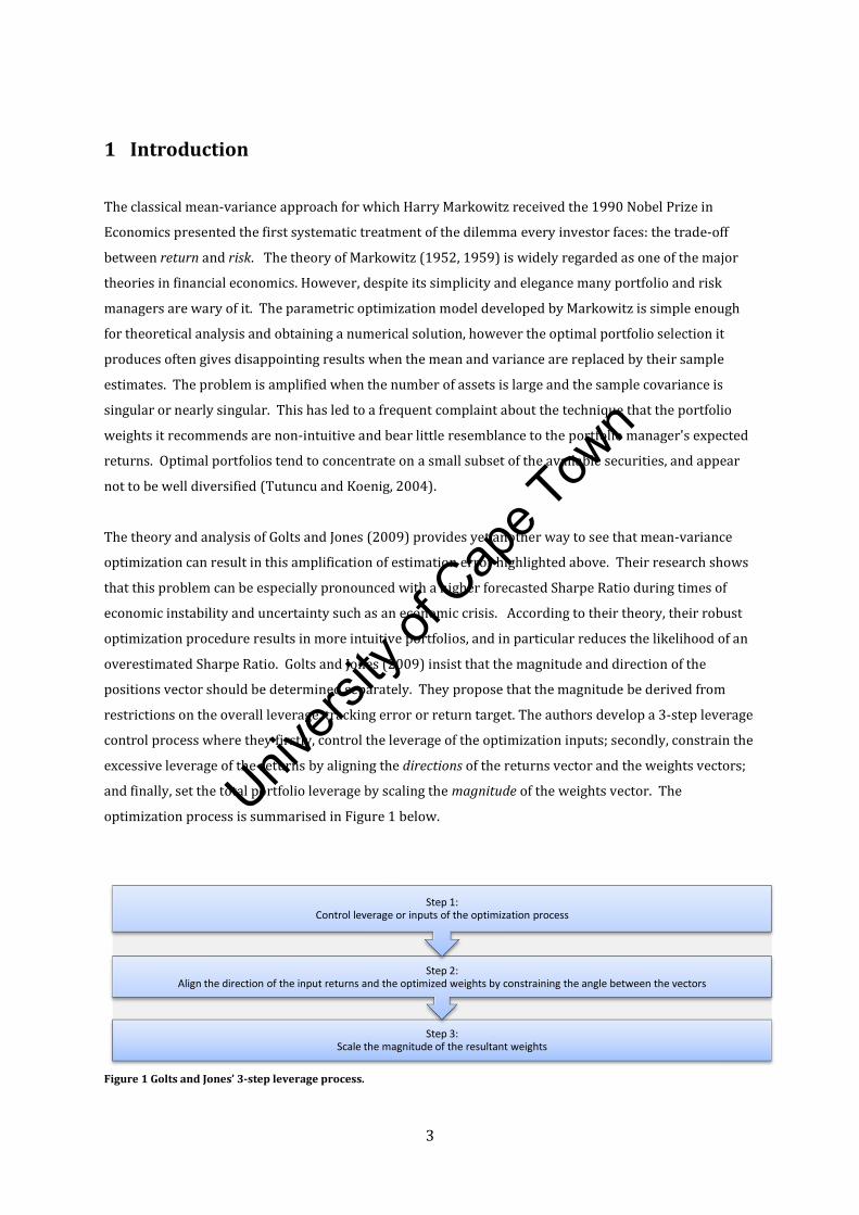
restrictions on the overall leverage, tracking error or return target. The authors develop a 3-step leverage
control process where they firstly, control the leverage of the optimization inputs; secondly, constrain the
excessive leverage of the returns by aligning the directions of the returns vector and the weights vectors;
and finally, set the total portfolio leverage by scaling the magnitude of the weights vector. The
optimization process is summarised in Figure 1 below.
Figure 1 Golts and Jones’ 3-step leverage process.
Step 3: Scale the magnitude of the resultant weights
Step 2: Align the direction of the input returns and the optimized weights by constraining the angle between the vectors
Step 1: Control leverage or inputs of the optimization process

Univers
ity of
Cap
e Tow
n
4
In this project, we explore the theory of the authors with the aim of demystifying the technique
mathematically. We also tackle and simplify the practical implementation of the technique. We then test
the validity of the 3-step leverage process of Golts and Jones (2009) using South African equity data. We
show that, indeed, the Golts and Jones (2009) theory results in an improvement in the straight-forward
Markowitz theory. Our findings suggest that applying their methodology to the South African equity
market results in portfolios with lower out-of-sample risk statistics. This mainly results from the new
robust covariance matrix being better-conditioned than the sample covariance matrix. In particular, we
find that the out-of-sample return is higher in times of economic instability and overall portfolio
performance is superior using this new robust methodology.
Univers
ity of
Cap
e Tow
n
5
2 Literature Review
Although more than half a century has passed since Markowitz's (1952) seminal work, the mean-variance
framework is still a key model used in practice today in asset allocation. The Markowitz efficient frontier
has also provided the foundation for many important advances in the area of financial economics,
including the Sharpe-Lintner and Capital Asset Pricing Model (CAPM) models. Under the framework of
Markowitz, the investor is concerned with the expected returns and the total risk of a static portfolio, and
should optimally hold the portfolio tangent to the efficient frontier.
In his ground-breaking theory, Markowitz made one very important assumption: that the investor has
foresight about the future performance of the asset returns. However, in practice these expected returns
have to be estimated as the investor does not have perfect foresight of the future performance of the
assets in question. It is also well-known that the expected returns are more difficult to estimate than the
covariance matrix, see Merton (1980). Chopra and Ziemba (1993) show that errors in the sample mean
estimate have a larger impact on the out-of-sample performance than errors in the sample covariance
estimate.
In addition to estimating the returns, solving the mean variance problem also requires estimating the
covariance matrix of returns and taking its inverse. This results in estimation error being amplified by
two factors. Estimation error is defined as the possibility of errors in the portfolio allocations due to
imprecision in the estimated inputs to the portfolio optimization (Jorian, 1992). Moreover, in practice,
the number of assets is typically very high and these asset returns may be highly correlated. A
culmination of all of these issues mentioned above will therefore result in an ill-posed problem when
even a slight change in one of the input parameters implies a significant change in the resultant portfolio
weights.
Many authors have highlighted the issue of the parameter uncertainty. Frankfurther, Seagle & Phillips
(1971) and Jobson & Korkie (1980) argue that, in fact, the portfolio based on sample estimates may not
be as effective as the equally weighted portfolio. Niedermayer and Zimmermann (2007) show, using
monte carlo simulation, that estimation error can cause strong deviations of the estimated portfolio
weights from the theoretically optimal weights. Golts and Jones (2009) argue that in practice “the ex-ante
Sharpe Ratio could be overestimated, and the resultant excessively high leverage could be very
dangerous”.
Over the years that followed, various authors have attempted to make improvements on the Markowitz
mean-variance optimization to tackle these issues. Some have used shrinkage, for example Ledoit and
Wolf (2004) argue that the sample covariance matrix should not be used for the purpose of portfolio
optimization because it contains significant estimation error. They propose to replace the covariance
matrix by a weighted average of the sample covariance and another structured matrix such as the identity
Univers
ity of
Cap
e Tow
n
6
matrix. Black and Litterman (1992) use reverse optimization, which uses portfolio weights (and the
covariance matrix) as input and provides expected returns as output to avoid the problem arising from
estimation error in expected returns. The aim of the Black Litterman model is to combine investors’
views with the equilibrium returns leading to potentially more stable optimal portfolios. Fama and
French (1993) show that risk factors other than the market factor should be taken into account. This has
led to the origination of the multifactor models. Advanced statistical methods such as principal
component analysis have also been applied in literature to extract explanatory factors from the historical
returns - however, this approach does not allow for factors that contain any real-world information that
can be easily distinguished from the estimation error. Lai, Xing and Chen (2009) propose a solution to a
stochastic optimization problem to extend Markowitz’s mean-variance portfolio optimization theory to
the case where the means and covariances of the asset returns for the next investment period are
unknown.
The Bayesian approach has also been widely recommended for dealing with the estimation errors in the
sample estimates. This method involves eliminating the dependence of the optimization process on the
true parameters by replacing them with a prior distribution of the fund manager’s view. Brown (1978)
shows that, the two-fund rule, which is the blend of the sample tangency portfolio and the risk-free asset,
is generally outperformed by the Bayesian decision rule under a given prior distribution. Kan and Zhou
(2007) also provide a theoretical demonstration of this result to show that the two-fund rule is often
suboptimal and outperformed by the Bayesian rule. They go further to propose a three-fund rule, which is
a combination between the two-fund rule and the global minimum variance portfolio which can yield
higher expected out-of-sample performance. However, the three-fund rule of Kan and Zhou (2007) has
some limitations: they make the assumption that returns are independent and identically distributed and
they do not deal with the case where there is a short-sale constraint in the optimization process.
Golts and Jones (2009) propose a completely new idea where the goal is to separate the direction and
magnitude of the portfolio positions vector. In their theory, they make no assumptions about the
distribution of the returns. Instead, they suggest making the covariance matrix better-conditioned
through a combination of robust portfolio optimization and Bayesian theory, thereby constraining the
angle between the vector of optimized weights and initial returns. This idea of robust portfolio
optimization is an emerging branch of research in the field of optimization. It has been explored
previously by authors such as Tutuncu and Konig (2004), Ceria and Stubbs (2006) and Scherer (2007)
who all demonstrate how robust portfolio optimization mitigates the problem of estimation error.
Robust optimization refers to finding solutions to given optimization problems with uncertain input
parameters that will achieve good objective values for all, or most, realizations of the uncertain input
parameters (Tutuncu and Koenig, 2004). The Golts and Jones (2009) theory proposes a new take on
robust optimization by insisting that the magnitude of the positions vector should be determined
separately, derived from restrictions on the overall leverage, tracking error, return target, or other

Univers
ity of
Cap
e Tow
n
7
possibly forward-looking considerations. This new outlook results in portfolios which are more intuitive
and which yield better out-of-sample performance.
Univers
ity of
Cap
e Tow
n
8
3 The classical mean-variance analysis with vector notation
In their 2009 paper, Golts and Jones dissect the theory of Markowitz at a more granular level. They
explore, separately, the direction and magnitude of the weights vector. This section delves into the ideas
brought forward in their research.
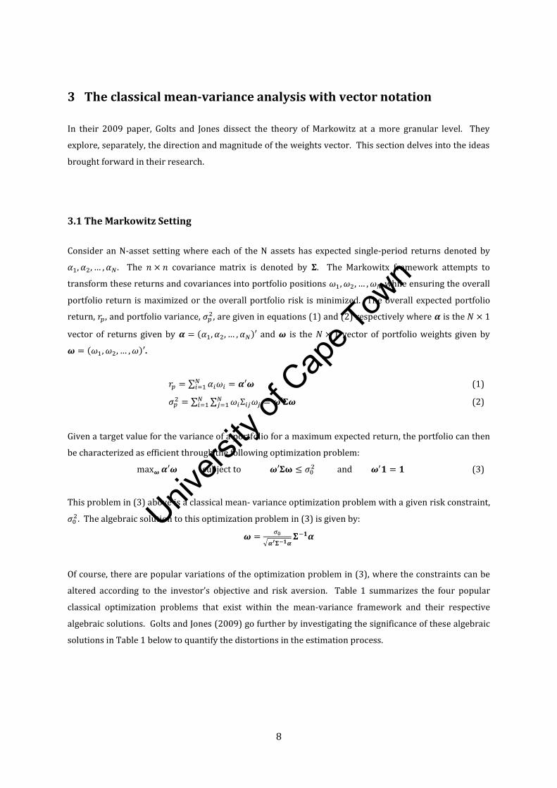
3.1 The Markowitz Setting
Consider an N-asset setting where each of the N assets has expected single-period returns denoted by
. The covariance matrix is denoted by . The Markowitx framework attempts to
transform these returns and covariances into portfolio positions while ensuring the overall
portfolio return is maximized or the overall portfolio risk is minimized. The overall expected portfolio
return, , and portfolio variance, , are given in equations (1) and (2) respectively where is the
vector of returns given by and is the vector of portfolio weights given by
.
(1)
(2)
Given a target value for the variance of a portfolio for a maximum expected return, the portfolio can then
be characterized as efficient through the following optimization problem:
subject to and (3)
This problem in (3) above is a classical mean- variance optimization problem with a given risk constraint,
. The algebraic solution to this optimization problem in (3) is given by:
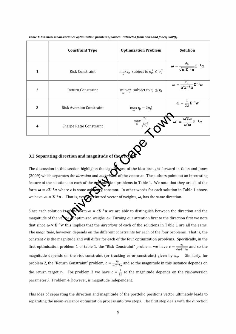
Of course, there are popular variations of the optimization problem in (3), where the constraints can be
altered according to the investor’s objective and risk aversion. Table 1 summarizes the four popular
classical optimization problems that exist within the mean-variance framework and their respective
algebraic solutions. Golts and Jones (2009) go further by investigating the significance of these algebraic
solutions in Table 1 below to quantify the distortions in the estimation process.
Univers
ity of
Cap
e Tow
n
9
Table 1: Classical mean-variance optimization problems (Source: Extracted from Golts and Jones(2009)).
Constraint Type
Optimization Problem
Solution
1
Risk Constraint
2
Return Constraint
3
Risk Aversion Constraint
4
Sharpe Ratio Constraint
3.2 Separating direction and magnitude of the vectors
The discussion in this section highlights the significance of the idea brought forward in Golts and Jones
(2009) which separates the direction and magnitude of the vector . The authors point out an interesting
feature of the solutions to each of the optimization problems in Table 1. We note that they are all of the
form where c is some arbitrary constant. In other words for each solution in Table 1 above,
we have . That is, every optimized vector of weights, , has the same direction.
Since each solution is of the form we are able to distinguish between the direction and the
magnitude of the vector of optimized weighs, . Turning our attention first to the direction first we note
that since this implies that the directions of each of the solutions in Table 1 are all the same.
The magnitude, however, depends on the different constraints for each of the four problems. That is, the
constant c is the magnitude and will differ for each of the four optimization problems. Specifically, in the
first optimisation problem 1 of table 1, the “Risk Constraint” problem, we have
and so the
magnitude depends on the risk constraint (or tracking error constraint) given by . Similarly, for
problem 2, the “Return Constraint” problem,
and so the magnitude in this instance depends on
the return target . For problem 3 we have
so the magnitude depends on the risk-aversion
parameter . Problem 4, however, is magnitude independent.
This idea of separating the direction and magnitude of the portfolio positions vector ultimately leads to
separating the mean-variance optimization process into two steps. The first step deals with the direction

Univers
ity of
Cap
e Tow
n
10
component while the second step focuses on the magnitude. Golts and Jones (2009) define the Investment
Direction by the unit vector given by
and the Investment Magnitude is defined by some norm of
, that is, by the leverage or the tracking error . The two-step process requires finding
the suitable direction so that thereafter “all magnitude decisions are simultaneously scalable”-(Golts and
Jones, 2009).
Univers
ity of
Cap
e Tow
n
11
4 The alpha-weight angle
Golts and Jones (2009) argue that in many instances the portfolios recommended by the Markowitz
framework are unintuitive. In other words, they bare very little resemblance to the fund manager’s
expectations of future portfolio performance. For this reason the vector of portfolio weights and the
vector of input returns can differ substantially. In order to quantify the difference between the returns
and resultant portfolio weights, they consider the angle between these two vectors.
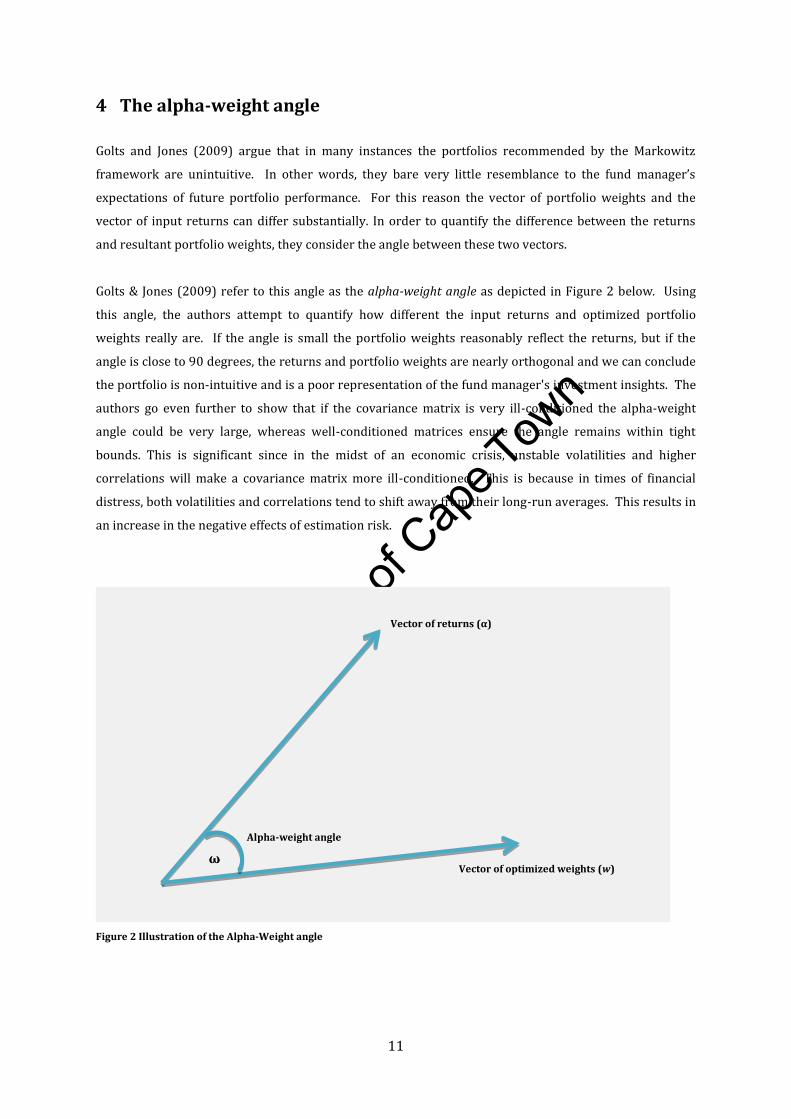
Golts & Jones (2009) refer to this angle as the alpha-weight angle as depicted in Figure 2 below. Using
this angle, the authors attempt to quantify how different the input returns and optimized portfolio
weights really are. If the angle is small the portfolio weights reasonably reflect the returns, but if the
angle is close to 90 degrees, the returns and portfolio weights are nearly orthogonal and we can conclude
the portfolio is non-intuitive and is a poor representation of the fund manager's investment insights. The
authors go even further to show that if the covariance matrix is very ill-conditioned the alpha-weight
angle could be very large, whereas well-conditioned matrices ensure the angle remains within tight
bounds. This is significant since in the midst of an economic crisis, unstable volatilities and higher
correlations will make a covariance matrix more ill-conditioned. This is because in times of financial
distress, both volatilities and correlations tend to shift away from their long-run averages. This results in
an increase in the negative effects of estimation risk.
Figure 2 Illustration of the Alpha-Weight angle
ω
Alpha-weight angle
Vector of returns (α)
Vector of optimized weights (w)
Univers
ity of
Cap
e Tow
n
12
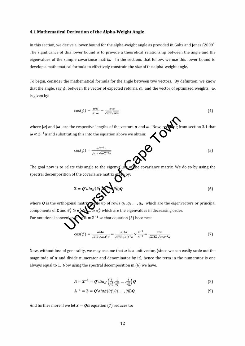
4.1 Mathematical Derivation of the Alpha-Weight Angle
In this section, we derive a lower bound for the alpha-weight angle as provided in Golts and Jones (2009).
The significance of this lower bound is to provide a theoretical relationship between the angle and the
eigenvalues of the sample covariance matrix. In the sections that follow, we use this lower bound to
develop a mathematical formula to effectively constrain the size of the alpha-weight angle.
To begin, consider the mathematical formula for the angle between two vectors. By definition, we know
that the angle, say , between the vector of expected returns, α, and the vector of optimized weights,
is given by:
(4)
where are the respective lengths of the vectors and . Now, recalling from section 3.1 that
and substituting this into the equation above we obtain:
(5)
The goal now is to relate this angle to the eigenvalues of the covariance matrix. We do so by using the
spectral decomposition of the covariance matrix given by:
(6)
where is the orthogonal matrix made up of rows which are the eigenvectors or principal
components of and
which are the eigenvalues in decreasing order.
For notational convenience let so that equation (5) becomes:
(7)
Now, without loss of generality, we may assume that is a unit vector, (since we can easily scale out the
magnitude of and divide numerator and denominator by it), hence the term in the numerator is one
always equal to 1. Now using the spectral decomposition in (6) we have:
(8)
(9)
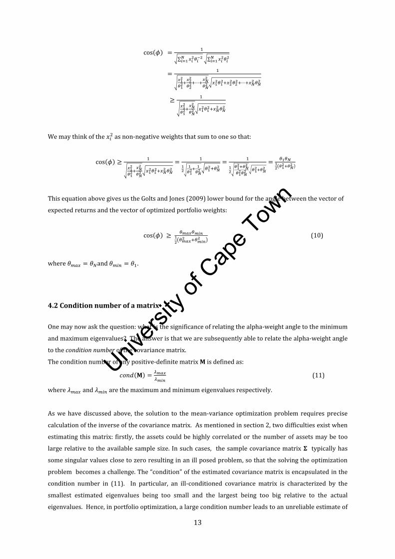
And further more if we let equation (7) reduces to:
Univers
ity of
Cap
e Tow
n
13
We may think of the as non-negative weights that sum to one so that:
This equation above gives us the Golts and Jones (2009) lower bound for the angle between the vector of
expected returns and the vector of optimized portfolio weights:
(10)
where .
4.2 Condition number of a matrix
One may now ask the question: what is the significance of relating the alpha-weight angle to the minimum
and maximum eigenvalues? The answer is that we are subsequently able to relate the alpha-weight angle
to the condition number of the covariance matrix.
The condition number of any positive-definite matrix is defined as:
(11)
where and are the maximum and minimum eigenvalues respectively.
As we have discussed above, the solution to the mean-variance optimization problem requires precise
calculation of the inverse of the covariance matrix. As mentioned in section 2, two difficulties exist when
estimating this matrix: firstly, the assets could be highly correlated or the number of assets may be too
large relative to the available sample size. In such cases, the sample covariance matrix typically has
some singular values close to zero resulting in an ill posed problem, so that the solving the optimization
problem becomes a challenge. The “condition” of the estimated covariance matrix is encapsulated in the
condition number in (11). In particular, an ill-conditioned covariance matrix is characterized by the
smallest estimated eigenvalues being too small and the largest being too big relative to the actual
eigenvalues. Hence, in portfolio optimization, a large condition number leads to an unreliable estimate of
Univers
ity of
Cap
e Tow
n
14
the vector of optimized portfolio weights. We can therefore use the condition number as an indication of
how well this inverse of the covariance matrix going into the optimization problem can be estimated. The
closer the condition number is to 1, the better conditioned the covariance matrix which implies its
inverse can be computed with good accuracy. If the condition number is large, then the matrix is said to
be ill-conditioned. In practice a covariance matrix with a large condition number is usually almost
singular, and the computation of its inverse is prone to large numerical errors.
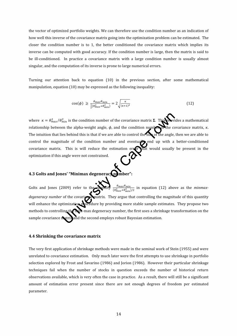
Turning our attention back to equation (10) in the previous section, after some mathematical
manipulation, equation (10) may be expressed as the following inequality:
(12)
where
is the condition number of the covariance matrix . This provides a mathematical
relationship between the alpha-weight angle, , and the condition number of the covariance matrix, .
The intuition that lies behind this is that if we are able to control the size of the angle, then we are able to
control the magnitude of the condition number and eventually end up with a better-conditioned
covariance matrix. This is will reduce the estimation error that would usually be present in the
optimization if this angle were not constrained.
4.3 Golts and Jones’ “Minimax degeneracy number”:
Golts and Jones (2009) refer to the quantity
in equation (12) above as the minmax-
degeneracy number of the covariance matrix. They argue that controlling the magnitude of this quantity
will enhance the optimization procedure by providing more stable sample estimates. They propose two
methods to controlling the mini-max degeneracy number, the first uses a shrinkage transformation on the
sample covariance matrix and the second employs robust Bayesian estimation.
4.4 Shrinking the covariance matrix
The very first application of shrinkage methods were made in the seminal work of Stein (1955) and were
unrelated to covariance estimation. Only much later were the first attempts to use shrinkage in portfolio
selection explored by Frost and Savarino (1986) and Jorion (1986). However their particular shrinkage
techniques fail when the number of stocks in question exceeds the number of historical return
observations available, which is very often the case in practice. As a result, there will still be a significant
amount of estimation error present since there are not enough degrees of freedom per estimated
parameter.

Univers
ity of
Cap
e Tow
n
15
Ledoit and Wolf (2003, 2004) propose an alternative method for dealing with the estimation error in the
covariance matrix by shrinking the covariance matrix obtained from the sample through a simple
transformation. This transformation assists in pulling the more extreme values toward more centralized
values and hence systematically reduces the estimation error. The crux of their shrinkage methodology is
that the estimated coefficients in the sample covariance matrix that are extremely high tend to contain a
lot of positive error. In other words, the most extreme coefficients in the sample covariance matrix tend
to take on such extreme values because they contain a significant amount of error. Invariably the mean-
variance optimization process will subsequently place its biggest bets on those coefficients which are the
most extremely unreliable. Michaud (1989) refers to this phenomenon “error- maximization”. Hence
these extreme covariances need to be decreased to compensate for that.
The shrinkage transformation of Ledoit and Wolf (2001) is the asymptotically optimal convex linear
combination of the sample covariance matrix with the identity matrix. This transformation is
distribution-free and has a simple formula that is easy to compute and interpret. The resultant
covariance estimator is both well-conditioned and more accurate than the sample covariance matrix.
Thus, shrinking these estimated covariance matrices towards an ideal structure will yield more stable
estimates as illustrated through Monte Carlo methods in Ledoit and Wolf (2001). The resulting
eigenvalues are more compressed, thus resulting in a condition number that is closer to unity eventually
leading to the covariance matrix estimate being better conditioned.
Hence, in the Golts and Jones (2009) framework, by shrinking the covariance matrix, we are able to
increase the “minimax degeneracy number” above and hence decrease the alpha-weight angle. We
consider the following shrinkage estimator:
(13)
where . The convex linear transformation in (13) averages the eigenvalues of the covariance
matrix and hence reduces the condition number (or equivalently decreases the size of the alpha-weight
angle).
This shrinkage estimator is one way of controlling, not only the condition number, mini-max degeneracy
number but more importantly the alpha-weight angle. In the next section we explore the alternative
method to constrain the alpha-weight angle dynamically.
Univers
ity of
Cap
e Tow
n
16
5 Robust optimization
Robust portfolio optimization refers to finding an optimization strategy where the behavior under the
worst possible realizations of the uncertain input parameters is optimized. Golts and Jones (2009)
introduce an innovative method for constraining the alpha-weight angle in the form of robust
optimization. In a robust setting, the returns are assumed to lie in some uncertainty region. In other
words, uncertainty is modelled by assuming that the input data is not known precisely, and will instead
lie in known sets.
Hence, in this robust setup, the optimization problem (3) becomes:
subject to (14)
where is the uncertainty region and is the given risk constraint.
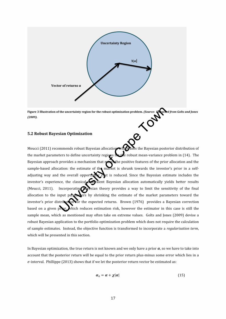
5.1 The uncertainty region
Goldfarb and Iyengar (2003) consider ellipsoidal uncertainty sets while Tutuncu and Koenig (2004)
prefer uncertainty intervals. To build on their theory Golts and Jones (2009) let the uncertainty region
be a sphere centred at with radius where lies between 0 and 1, as illustrated in Figure 3. By
setting the uncertainty region to be a sphere, we can now apply Bayesian theory to solve the optimization
problem. This method is discussed in the next section.
Univers
ity of
Cap
e Tow
n
17
Figure 3 Illustration of the uncertainty region for the robust optimization problem. (Source: Extracted from Golts and Jones
(2009).
5.2 Robust Bayesian Optimization
Meucci (2011) recommends robust Bayesian allocation, which uses the Bayesian posterior distribution of
the market parameters to define uncertainty regions for the robust mean-variance problem in (14). The
Bayesian approach provides a mechanism that mixes the positive features of the prior allocation and the
sample-based allocation: the estimate of the market is shrunk towards the investor’s prior in a self-
adjusting way and the overall opportunity cost is reduced. Since the Bayesian estimate includes the
investor’s experience, the classical-equivalent Bayesian allocation automatically yields better results
(Meucci, 2011). Incorporating Bayesian theory provides a way to limit the sensitivity of the final
allocation to the input parameters by shrinking the estimate of the market parameters toward the
investor’s prior distribution for the expected returns. Brown (1976) provides a Bayesian correction
based on a given prior, which reduces estimation risk, however the estimator in this case is still the
sample mean, which as mentioned may often take on extreme values. Golts and Jones (2009) devise a
robust Bayesian application to the portfolio optimization problem which does not require the calculation
of sample estimates. Instead, the objective function is transformed to incorporate a regularisation term,
which will be presented in this section.
In Bayesian optimization, the true return is not known and we only have a prior , so we have to take into
account that the posterior return will be equal to the prior return plus-minus some error which lies in a
-interval. Phillippe (2013) shows that if we let the posterior return vector be estimated as:
(15)
Vector of returns α
Χ|α|
Uncertainty Region
Univers
ity of
Cap
e Tow
n
18
with or equivalenty then this exactly describes a sphere around . The portfolio return is
then given by:
(16)
So to find the worst-case return within this sphere, we need to minimize the function in (17). The first
term is a constant. So we want to reduce that as much as possible. From the second term is also
just a constant, hence we are looking for the smallest value of .
We may write where is the angle between the two vectors. So, we see that setting
will minimize the portfolio return, , in (17). And so we end up with:
(17)
for . We may now bring the alpha-weight angle into this equation such that
(18)
Doing this allows us to simplify the robust optimization problem to a standard optimization problem
which now includes a regularization term given by . The strength of this regularization term is
controlled by the factor . This factor penalizes angles for being less acute.
The robust Bayesian optimization problem in for the spherical uncertainty region, , can be defined
mathematically as:
subject to
(19)
The algebraic solution to this optimization problem, as provided in Golts and Jones (2009) is:
(20)
where is the norm of the vector of expected returns, .
Golts and Jones (2009) also provide the formula for the robust covariance matrix family as:
(21)
Univers
ity of
Cap
e Tow
n
19
Hence we see that equation (21) shrinks the actual covariance matrix in a similar way as equation (13)
and the robust covariance matrix is now conditional on .
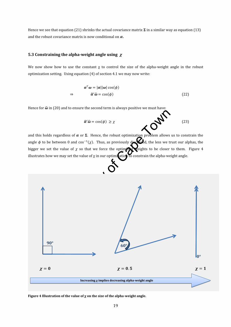
5.3 Constraining the alpha-weight angle using
We now show how to use the constant χ to control the size of the alpha-weight angle in the robust
optimization setting. Using equation (4) of section 4.1 we may now write:
(22)
Hence for in (20) and to ensure the second term is always positive we must have:
(23)
and this holds regardless of or . Hence, the robust optimization problem allows us to constrain the
angle to be between 0 and . Thus, as previously discussed, the less we trust our alphas, the
bigger we set the value of so that we force the optimized weights to be closer to them. Figure 4
illustrates how we may set the value of χ in our optimization to constrain the alpha-weight angle.
Figure 4 Illustration of the value of χ on the size of the alpha-weight angle.
0°
90° 60°
Increasing χ implies decreasing alpha-weight angle

Univers
ity of
Cap
e Tow
n
20
6 Practical Implementation of the technique
Implementation of the Golts and Jones (2009) robust optimization requires solid breakdown of the
optimization problem in question. As discussed in section 3 above, if there are no upper or lower bound
constraints on the weights then problems 1-4 in Table 1 all have the same directional solution.
Implementation of the technique therefore requires minimization over the uncertainty region of section
5.1. There are two approaches to minimizing within the uncertainty region. The first method is the N-
dimensional optimization and the second is to run the optimization using the spherical symmetry of the
uncertainty region. In this section we discuss both methods.
6.1 N-dimensional optimization
Section 5.2 has simplified the robust optimization problem in (14) to now be:
(24)
In this case, we are merely solving for the directional component, .
The value of in (24) can be set between 0 and 1 depending on how much we want to constrain the angle.
The closer is to 1, the less we allow the angle to widen. The value of is set at the start of the
optimization and remains constant throughout.
This N-dimensional optimization problem will also allow us to use the nonlinear inequality constraint
given by:
(25)
where most programming software is equipped to handle this problem. For example, Matlab’s built-in
fmincon function can handle this using the 'active-set' algorithm. However, if we wish to
optimize on the strict sphere so that we have the equality constraint:
(26)
then it would be better to use Matlab’s fmincon using the interior point' algorithm – although
this may be less inefficient. We then simply run fmincon using the Golts and Jones (2009) objective
function subject to a given tracking error or risk constraint. We find that the use of an equality constraint
for the tracking error to work best for this optimization as it results in solution which is always an
interior one.
If there are upper and lower bound constraints in the optimization then an important consideration for
employing the optimization is that we need to scale our initial weights to “honor” this constraint. The
Univers
ity of
Cap
e Tow
n
21
basic idea on scaling the initial point is that for certain types of optimization algorithms the initial point
needs to be feasible in terms of the constraints. This is primarily because the way constraints get folded
into the Lagranian (extended objective function) is via a logarithmic barrier. This simply means that we
cannot get through the barrier from infeasible point to feasible point, or vice versa. In Matlab
particularly, if we start with an infeasible point we cannot necessarily get to a feasible point using the
fmincon function. Hence, we need to start by trying to generate a point from the objective function. We
find that using Matlab’s pinv to find an initial vector of weights works well.
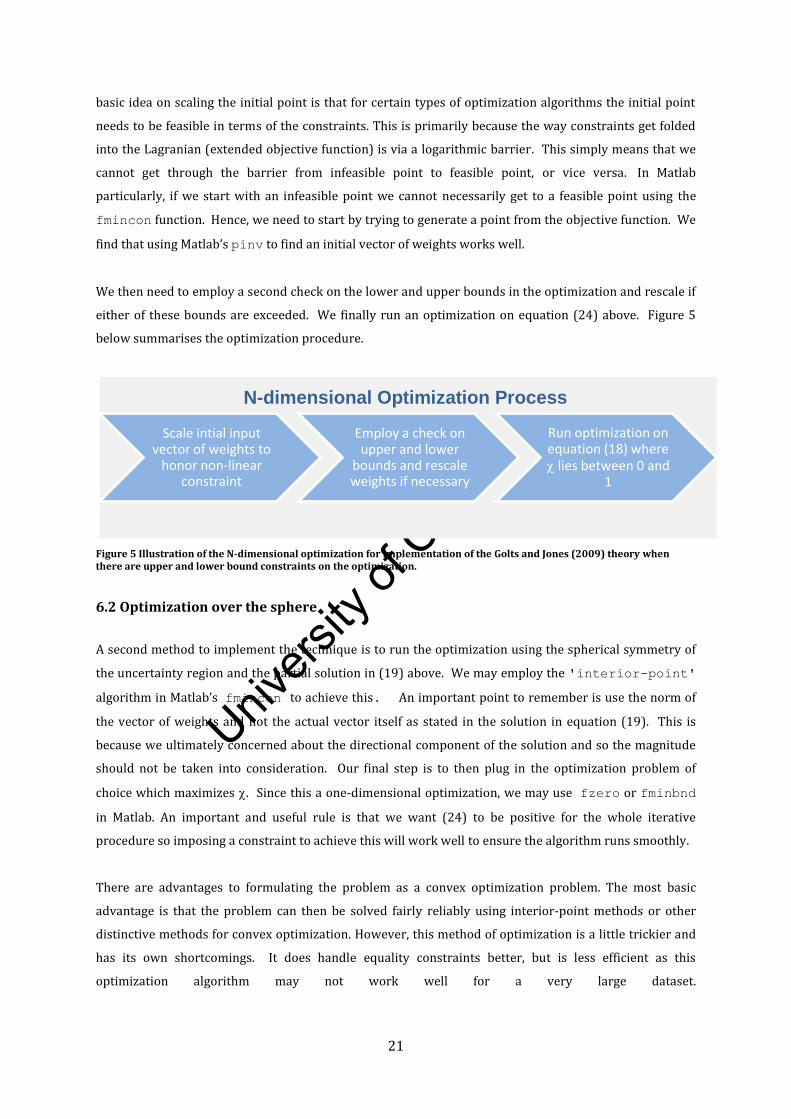
We then need to employ a second check on the lower and upper bounds in the optimization and rescale if
either of these bounds are exceeded. We finally run an optimization on equation (24) above. Figure 5
below summarises the optimization procedure.
Figure 5 Illustration of the N-dimensional optimization for implementation of the Golts and Jones (2009) theory when there are upper and lower bound constraints on the optimization.
6.2 Optimization over the sphere
A second method to implement the technique is to run the optimization using the spherical symmetry of
the uncertainty region and the partial solution in (19) above. We may employ the 'interior-point'
algorithm in Matlab’s fmincon to achieve this. An important point to remember is use the norm of
the vector of weights and not the actual vector itself as stated in the solution in equation (19). This is
because we ultimately concerned about the directional component of the solution and so the magnitude
should not be taken into consideration. Our final step is to then plug in the optimization problem of
choice which maximizes . Since this a one-dimensional optimization, we may use fzero or fminbnd
in Matlab. An important and useful rule is that we want (24) to be positive for the whole iterative
procedure so imposing a constraint to achieve this will work well to ensure the algorithm runs smoothly.
There are advantages to formulating the problem as a convex optimization problem. The most basic
advantage is that the problem can then be solved fairly reliably using interior-point methods or other
distinctive methods for convex optimization. However, this method of optimization is a little trickier and
has its own shortcomings. It does handle equality constraints better, but is less efficient as this
optimization algorithm may not work well for a very large dataset.
Scale intial input vector of weights to
honor non-linear constraint
Employ a check on upper and lower
bounds and rescale weights if necessary
Run optimization on equation (18) where lies between 0 and
1
N-dimensional Optimization Process
Univers
ity of
Cap
e Tow
n
22
7 Empirical analysis
In this section, we aim to test the Golts and Jones (2009) theory in the South African equity market. We
apply the robust optimization theory and compare the results obtained to the straight-forward
Markowitz method as well as the shrinkage method of section 4.4.
7.1 Data
We use weekly data on shares listed on the All Share Index (ALSI) of the Johannesburg Stock Exchange
(JSE). The ALSI contains 164 securities listed on the JSE and represents 99% of the full market capital.
For our analysis, we use ALSI data for the period January 2002 to July 2012, sourced from the I-Net
Bridge database. At each month end, we find the largest 100 shares on the ALSI and use those shares in
our sample. In some instances, there may have been shares with similar weights and in such instances we
include all those shares and would therefore have slightly more than 100 shares in our sample. Because
we use the top 100 shares in the ALSI at each month end, we have (almost) no survivorship bias. As our
benchmark in the analysis, we extract the relevant set of returns from the data above to form the
constituents of the benchmark at each specified date.
7.2 Methodology
We run a back-testing algorithm to compare the results obtained between three different scenarios,
namely:
CASE 1: the Markowitz theory using the sample covariance matrix;
CASE 2: the Markowitz theory using the shrunk-to-average covariance estimator in
equation (13) where a factor of 0.5 is used to blend the sample covariance
matrix and the shrunk-to-average covariance matrix. We choose this factor to
obtain an equally weighted covariance matrix as done in the literature, see for
example, Le Doit and Wolf (2003)).
CASE 3: the robust Bayesian optimization algorithm of where we set our value of χ at 0.5
so that the alpha-weight angle is constrained to 60°, similar to the analysis
employed in Golts and Jones (2009). We set χ at this value so as not to be too
stringent on the alpha-weight angle.
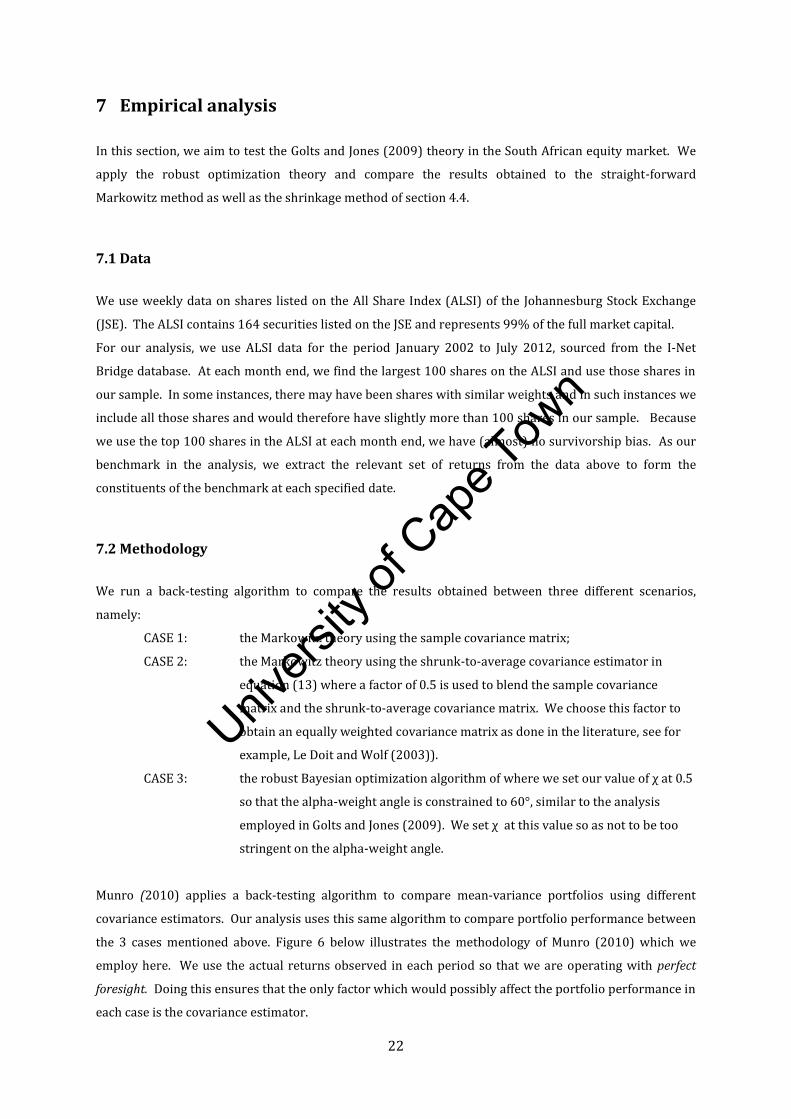
Munro (2010) applies a back-testing algorithm to compare mean-variance portfolios using different
covariance estimators. Our analysis uses this same algorithm to compare portfolio performance between
the 3 cases mentioned above. Figure 6 below illustrates the methodology of Munro (2010) which we
employ here. We use the actual returns observed in each period so that we are operating with perfect
foresight. Doing this ensures that the only factor which would possibly affect the portfolio performance in
each case is the covariance estimator.
Univers
ity of
Cap
e Tow
n
23
Figure 6 Illustration of the back-testing methodology used in the analysis. (Source: Adapted from Munro (2010))
We estimate covariance matrices using 3 years (or 170 weekly returns) worth of data between January
2002 and December 2005. In order to calculate the covariance matrix, all stocks need to have a full
history of data – however in most real-world applications this often is not always the case. To cater for
stocks where data availability was an issue, the missing data is replaced with the return of the stocks’
sector as a proxy for its actual return.
We then run the optimization algorithm from January 2005 and allow a 1 month hold-out period between
January 2005 and February 2005. We then move forward one month and repeat this process until July
2012. To calculate the covariance matrices, we use the following methodology for each of the cases
described above:
CASE 1: we use the sample covariance matrix is estimated using the historical data
between January 2002 to December 2004,
CASE 2: we use the sample covariance matrix in CASE 1 above and shrink it to the
average covariances,
CASE 3: the sample covariance matrix is fed into the optimization algorithm.
For all 3 cases above, we apply a 4% tracking error constraint throughout the time period. We use
fmincon in Matlab to implement the mean-variance optimization in case 1 and case 2 as well as the N-
dimensional optimization routine for case 3.
7.3 Results
7.3.1 Covariance Matrices
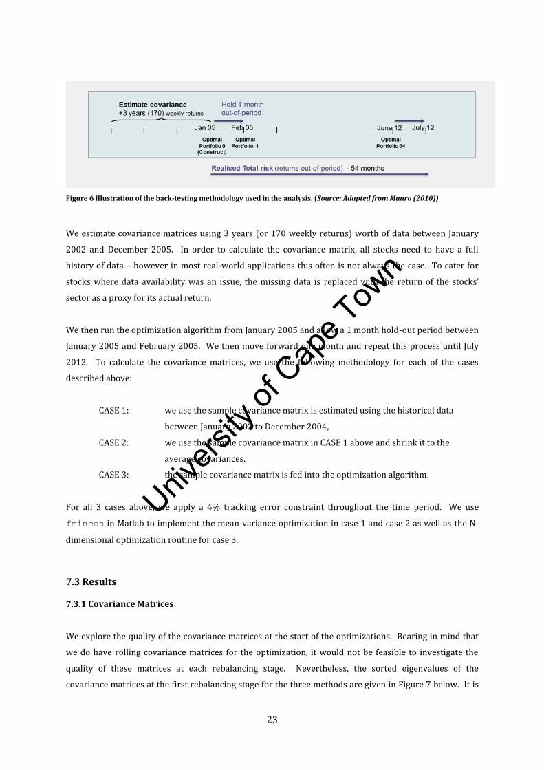
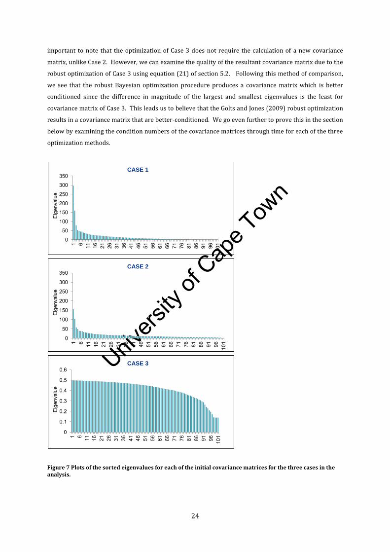
We explore the quality of the covariance matrices at the start of the optimizations. Bearing in mind that
we do have rolling covariance matrices for the optimization, it would not be feasible to investigate the
quality of these matrices at each rebalancing stage. Nevertheless, the sorted eigenvalues of the
covariance matrices at the first rebalancing stage for the three methods are given in Figure 7 below. It is
Univers
ity of
Cap
e Tow
n
24
important to note that the optimization of Case 3 does not require the calculation of a new covariance
matrix, unlike Case 2. However, we can examine the quality of the resultant covariance matrix due to the
robust optimization of Case 3 using equation (21) of section 5.2. Following this method of comparison,
we see that the robust Bayesian optimization procedure produces a covariance matrix which is better
conditioned since the difference in magnitude of the largest and smallest eigenvalues is the least for
covariance matrix of Case 3. This leads us to believe that the Golts and Jones (2009) robust optimization
results in a covariance matrix that are better-conditioned. We go even further to prove this in the section
below by examining the condition numbers of the covariance matrices through time for each of the three
optimization methods.
Figure 7 Plots of the sorted eigenvalues for each of the initial covariance matrices for the three cases in the analysis.
0
50
100
150
200
250
300
350
1 6 11
16
21
26
31
36
41
46
51
56
61
66
71
76
81
86
91
96
101
Eig
enva
lue
CASE 1
0
50
100
150
200
250
300
350
1 6 11
16
21
26
31
36
41
46
51
56
61
66
71
76
81
86
91
96
101
Eig
enva
lue
CASE 2
0
0.1
0.2
0.3
0.4
0.5
0.6
1 6 11
16
21
26
31
36
41
46
51
56
61
66
71
76
81
86
91
96
101
Eig
enva
lue
CASE 3
Univers
ity of
Cap
e Tow
n
25
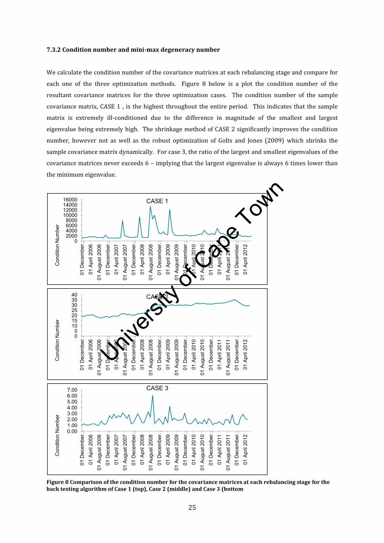
7.3.2 Condition number and mini-max degeneracy number
We calculate the condition number of the covariance matrices at each rebalancing stage and compare for
each one of the three optimization methods. Figure 8 below is a plot the condition number of the
resultant covariance matrices for the three optimization cases. The condition number of the sample
covariance matrix, CASE 1 , is the highest throughout the entire period. This indicates that the sample
matrix is extremely ill-conditioned due to the difference in magnitude of the smallest and largest
eigenvalue being extremely high. The shrinkage method of CASE 2 significantly improves the condition
number, however not as well as the robust optimization of Golts and Jones (2009) which shrinks the
sample covariance matrix dynamically. For case 3, the ratio of the largest and smallest eigenvalues of the
covariance matrices never exceeds 6 – implying that the largest eigenvalue is always 6 times lower than
the minimum eigenvalue.
Figure 8 Comparison of the condition number for the covariance matrices at each rebalancing stage for the back testing algorithm of Case 1 (top), Case 2 (middle) and Case 3 (bottom
0 2000 4000 6000 8000
10000 12000 14000 16000
01 D
ecem
ber …
01
Apr
il 20
06
01 A
ugus
t 200
6 01
Dec
embe
r …
01 A
pril
2007
01
Aug
ust 2
007
01 D
ecem
ber …
01
Apr
il 20
08
01 A
ugus
t 200
8 01
Dec
embe
r …
01 A
pril
2009
01
Aug
ust 2
009
01 D
ecem
ber …
01
Apr
il 20
10
01 A
ugus
t 201
0 01
Dec
embe
r …
01 A
pril
2011
01
Aug
ust 2
011
01 D
ecem
ber …
01
Apr
il 20
12
Con
ditio
n N
umbe
r
CASE 1
0 5
10 15 20 25 30 35 40
01 D
ecem
ber …
01
Apr
il 20
06
01 A
ugus
t 200
6 01
Dec
embe
r …
01 A
pril
2007
01
Aug
ust 2
007
01 D
ecem
ber …
01
Apr
il 20
08
01 A
ugus
t 200
8 01
Dec
embe
r …
01 A
pril
2009
01
Aug
ust 2
009
01 D
ecem
ber …
01
Apr
il 20
10
01 A
ugus
t 201
0 01
Dec
embe
r …
01 A
pril
2011
01
Aug
ust 2
011
01 D
ecem
ber …
01
Apr
il 20
12
Con
ditio
n N
umbe
r
CASE 2
0.00 1.00 2.00 3.00 4.00 5.00 6.00 7.00
01 D
ecem
ber …
01
Apr
il 20
06
01 A
ugus
t 200
6 01
Dec
embe
r …
01 A
pril
2007
01
Aug
ust 2
007
01 D
ecem
ber …
01
Apr
il 20
08
01 A
ugus
t 200
8 01
Dec
embe
r …
01 A
pril
2009
01
Aug
ust 2
009
01 D
ecem
ber …
01
Apr
il 20
10
01 A
ugus
t 201
0 01
Dec
embe
r …
01 A
pril
2011
01
Aug
ust 2
011
01 D
ecem
ber …
01
Apr
il 20
12
Con
ditio
n N
umbe
r
CASE 3
Univers
ity of
Cap
e Tow
n
26
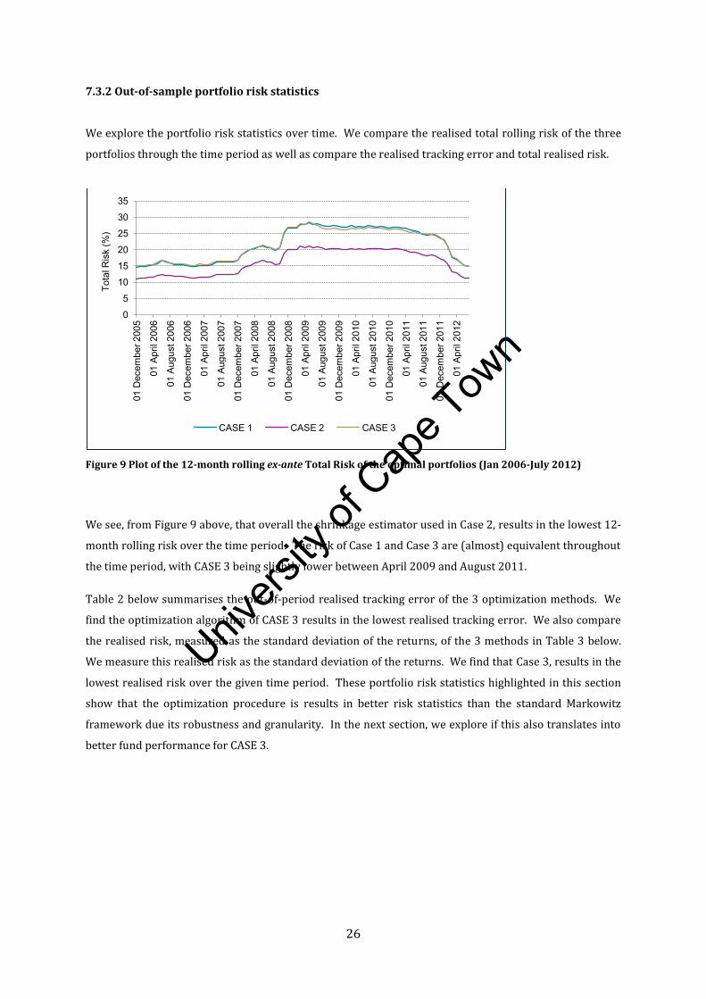
7.3.2 Out-of-sample portfolio risk statistics
We explore the portfolio risk statistics over time. We compare the realised total rolling risk of the three
portfolios through the time period as well as compare the realised tracking error and total realised risk.
Figure 9 Plot of the 12-month rolling ex-ante Total Risk of the optimal portfolios (Jan 2006-July 2012)
We see, from Figure 9 above, that overall the shrinkage estimator used in Case 2, results in the lowest 12-
month rolling risk over the time period. The risk of Case 1 and Case 3 are (almost) equivalent throughout
the time period, with CASE 3 being slightly lower between April 2009 and August 2011.
Table 2 below summarises the out-of-period realised tracking error of the 3 optimization methods. We
find the optimization algorithm of CASE 3 results in the lowest realised tracking error. We also compare
the realised risk, measured as the standard deviation of the returns, of the 3 methods in Table 3 below.
We measure this realised risk as the standard deviation of the returns. We find that Case 3, results in the
lowest realised risk over the given time period. These portfolio risk statistics highlighted in this section
show that the optimization procedure is results in better risk statistics than the standard Markowitz
framework due its robustness and granularity. In the next section, we explore if this also translates into
better fund performance for CASE 3.
0
5
10
15
20
25
30
35
01 D
ecem
ber 2
005
01 A
pril
2006
01 A
ugus
t 200
6
01 D
ecem
ber 2
006
01 A
pril
2007
01 A
ugus
t 200
7
01 D
ecem
ber 2
007
01 A
pril
2008
01 A
ugus
t 200
8
01 D
ecem
ber 2
008
01 A
pril
2009
01 A
ugus
t 200
9
01 D
ecem
ber 2
009
01 A
pril
2010
01 A
ugus
t 201
0
01 D
ecem
ber 2
010
01 A
pril
2011
01 A
ugus
t 201
1
01 D
ecem
ber 2
011
01 A
pril
2012
Tota
l Ris
k (%
)
CASE 1 CASE 2 CASE 3
Univers
ity of
Cap
e Tow
n
27
Table 2 Out-of-period tracking error of the optimal portfolios (January 2006-July 2012)
Tracking error to ALSI
Average TE (In-period)
Realised TE (Out-of-period)
CASE 1 4% 5.3%
CASE 2 4% 5.2%
CASE 3 4% 5.1%
Table 3 Out-of-period realised risk, or standard deviation of the returns, of the optimal portfolios (January 2006-July 2012)
Realised Total Risk (Standard deviation of the returns)
CASE 1 18.41
CASE 2 18.10
CASE 3 17.57
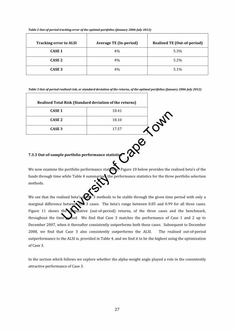
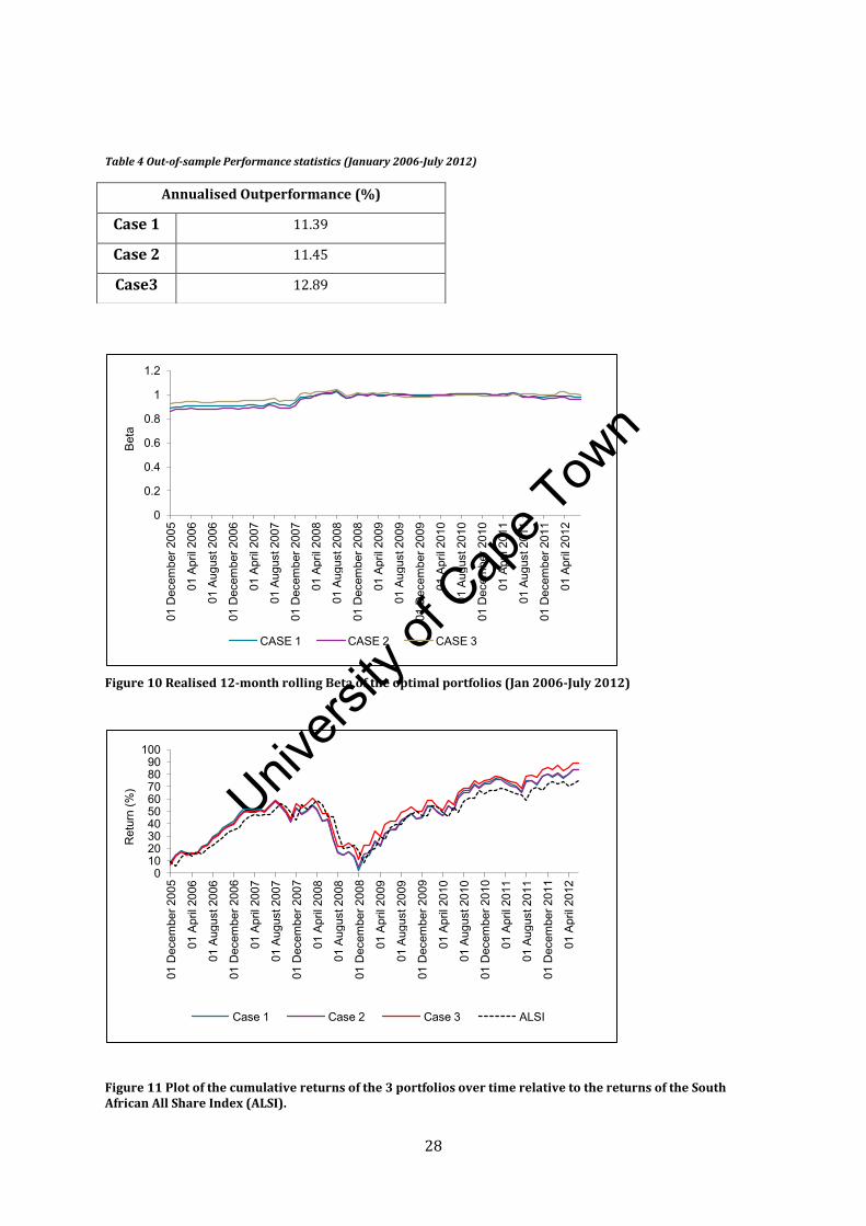
7.3.3 Out-of-sample portfolio performance statistics
We now examine the portfolio performance statistics. Figure 10 below provides the realised beta’s of the
funds through time while Table 4 summarises the performance statistics for the three portfolio selection
methods.
We see that the realised beta’s of the 3 methods to be stable through the given time period with only a
marginal difference between the 3 cases. The beta’s range between 0.85 and 0.99 for all three cases.
Figure 11 shows the cumulative (out-of-period) returns, of the three cases and the benchmark,
throughout the time period. We find that Case 3 matches the performance of Case 1 and 2 up to
December 2007, when it thereafter consistently outperforms both these cases. Subsequent to December
2008, we find that Case 3 also consistently outperforms the ALSI. The realised out-of-period
outperformance to the ALSI is, provided in Table 4, and we find it to be the highest using the optimization
of Case 3.
In the section which follows we explore whether the alpha-weight angle played a role in the consistently
attractive performance of Case 3.
Univers
ity of
Cap
e Tow
n
28
Table 4 Out-of-sample Performance statistics (January 2006-July 2012)
Figure 10 Realised 12-month rolling Beta of the optimal portfolios (Jan 2006-July 2012)
Figure 11 Plot of the cumulative returns of the 3 portfolios over time relative to the returns of the South African All Share Index (ALSI).
0
0.2
0.4
0.6
0.8
1
1.2
01 D
ecem
ber 2
005
01 A
pril
2006
01 A
ugus
t 200
6
01 D
ecem
ber 2
006
01 A
pril
2007
01 A
ugus
t 200
7
01 D
ecem
ber 2
007
01 A
pril
2008
01 A
ugus
t 200
8
01 D
ecem
ber 2
008
01 A
pril
2009
01 A
ugus
t 200
9
01 D
ecem
ber 2
009
01 A
pril
2010
01 A
ugus
t 201
0
01 D
ecem
ber 2
010
01 A
pril
2011
01 A
ugus
t 201
1
01 D
ecem
ber 2
011
01 A
pril
2012
Bet
a
CASE 1 CASE 2 CASE 3
0 10 20 30 40 50 60 70 80 90
100
01 D
ecem
ber 2
005
01 A
pril
2006
01 A
ugus
t 200
6
01 D
ecem
ber 2
006
01 A
pril
2007
01 A
ugus
t 200
7
01 D
ecem
ber 2
007
01 A
pril
2008
01 A
ugus
t 200
8
01 D
ecem
ber 2
008
01 A
pril
2009
01 A
ugus
t 200
9
01 D
ecem
ber 2
009
01 A
pril
2010
01 A
ugus
t 201
0
01 D
ecem
ber 2
010
01 A
pril
2011
01 A
ugus
t 201
1
01 D
ecem
ber 2
011
01 A
pril
2012
Ret
urn
(%)
Case 1 Case 2 Case 3 ALSI
Annualised Outperformance (%)
Case 1 11.39
Case 2 11.45
Case3 12.89
Univers
ity of
Cap
e Tow
n
29
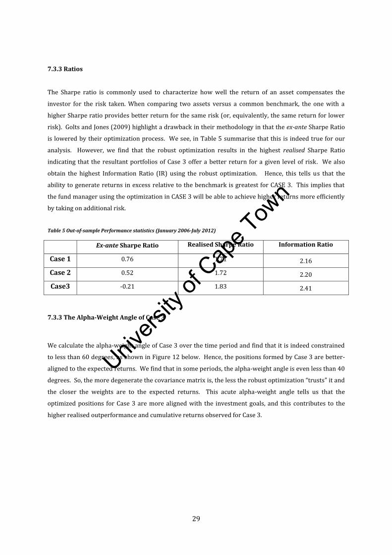
7.3.3 Ratios
The Sharpe ratio is commonly used to characterize how well the return of an asset compensates the
investor for the risk taken. When comparing two assets versus a common benchmark, the one with a
higher Sharpe ratio provides better return for the same risk (or, equivalently, the same return for lower
risk). Golts and Jones (2009) highlight a drawback in their methodology in that the ex-ante Sharpe Ratio
is lowered by their optimization process. We see, in Table 5 summarise that this is indeed true for our
analysis. However, we find that the robust optimization results in the highest realised Sharpe Ratio
indicating that the resultant portfolios of Case 3 offer a better return for a given level of risk. We also
obtain the highest Information Ratio (IR) using the robust optimization. Hence, this tells us that the
ability to generate returns in excess relative to the benchmark is greatest for CASE 3. This implies that
the fund manager using the optimization in CASE 3 will be able to achieve higher returns more efficiently
by taking on additional risk.
Table 5 Out-of-sample Performance statistics (January 2006-July 2012)
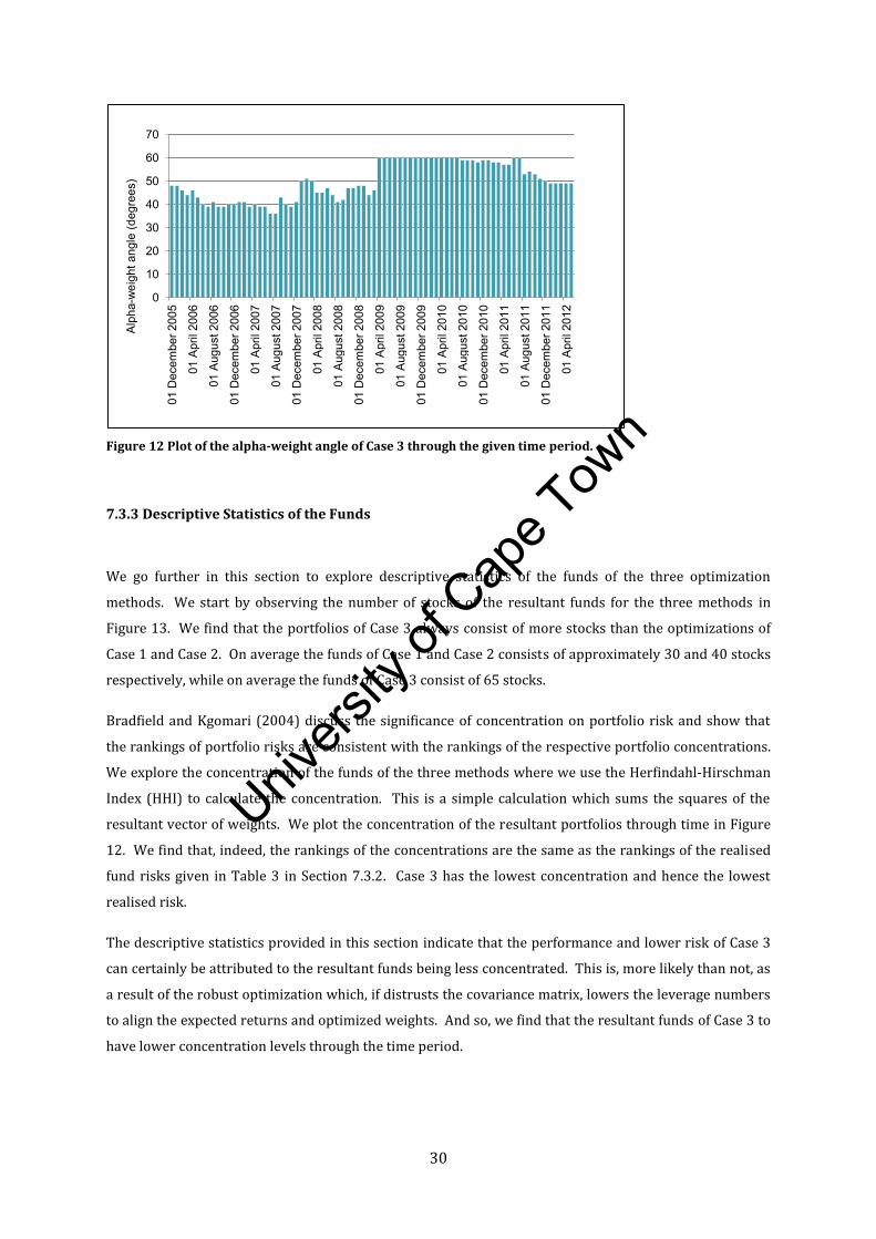
7.3.3 The Alpha-Weight Angle of Case 3
We calculate the alpha-weight angle of Case 3 over the time period and find that it is indeed constrained
to less than 60 degrees, as shown in Figure 12 below. Hence, the positions formed by Case 3 are better-
aligned to the expected returns. We find that in some periods, the alpha-weight angle is even less than 40
degrees. So, the more degenerate the covariance matrix is, the less the robust optimization “trusts” it and
the closer the weights are to the expected returns. This acute alpha-weight angle tells us that the
optimized positions for Case 3 are more aligned with the investment goals, and this contributes to the
higher realised outperformance and cumulative returns observed for Case 3.
Ex-ante Sharpe Ratio Realised Sharpe Ratio Information Ratio
Case 1 0.76 1.71 2.16
Case 2 0.52 1.72 2.20
Case3 -0.21 1.83 2.41
Univers
ity of
Cap
e Tow
n
30
Figure 12 Plot of the alpha-weight angle of Case 3 through the given time period.
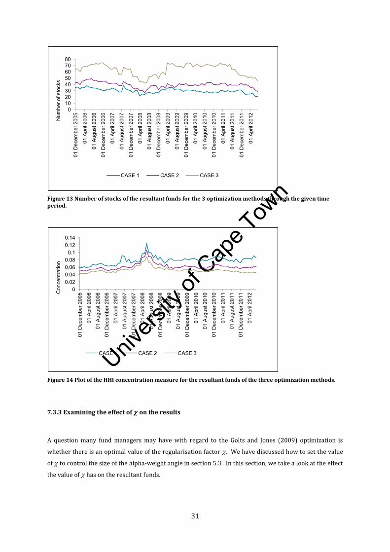
7.3.3 Descriptive Statistics of the Funds
We go further in this section to explore descriptive statistics of the funds of the three optimization
methods. We start by observing the number of stocks of the resultant funds for the three methods in
Figure 13. We find that the portfolios of Case 3 always consist of more stocks than the optimizations of
Case 1 and Case 2. On average the funds of Case 1 and Case 2 consists of approximately 30 and 40 stocks
respectively, while on average the funds of Case 3 consist of 65 stocks.
Bradfield and Kgomari (2004) discuss the significance of concentration on portfolio risk and show that
the rankings of portfolio risks are consistent with the rankings of the respective portfolio concentrations.
We explore the concentration of the funds of the three methods where we use the Herfindahl-Hirschman
Index (HHI) to calculate the concentration. This is a simple calculation which sums the squares of the
resultant vector of weights. We plot the concentration of the resultant portfolios through time in Figure
12. We find that, indeed, the rankings of the concentrations are the same as the rankings of the realised
fund risks given in Table 3 in Section 7.3.2. Case 3 has the lowest concentration and hence the lowest
realised risk.
The descriptive statistics provided in this section indicate that the performance and lower risk of Case 3
can certainly be attributed to the resultant funds being less concentrated. This is, more likely than not, as
a result of the robust optimization which, if distrusts the covariance matrix, lowers the leverage numbers
to align the expected returns and optimized weights. And so, we find that the resultant funds of Case 3 to
have lower concentration levels through the time period.
0
10
20
30
40
50
60
70
01 D
ecem
ber 2
005
01 A
pril
2006
01 A
ugus
t 200
6
01 D
ecem
ber 2
006
01 A
pril
2007
01 A
ugus
t 200
7
01 D
ecem
ber 2
007
01 A
pril
2008
01 A
ugus
t 200
8
01 D
ecem
ber 2
008
01 A
pril
2009
01 A
ugus
t 200
9
01 D
ecem
ber 2
009
01 A
pril
2010
01 A
ugus
t 201
0
01 D
ecem
ber 2
010
01 A
pril
2011
01 A
ugus
t 201
1
01 D
ecem
ber 2
011
01 A
pril
2012
Alp
ha-w
eigh
t ang
le (d
egre
es)
Univers
ity of
Cap
e Tow
n
31
Figure 13 Number of stocks of the resultant funds for the 3 optimization methods through the given time period.
Figure 14 Plot of the HHI concentration measure for the resultant funds of the three optimization methods.
7.3.3 Examining the effect of on the results
A question many fund managers may have with regard to the Golts and Jones (2009) optimization is
whether there is an optimal value of the regularisation factor . We have discussed how to set the value
of to control the size of the alpha-weight angle in section 5.3. In this section, we take a look at the effect
the value of has on the resultant funds.
0 10 20 30 40 50 60 70 80
01 D
ecem
ber 2
005
01 A
pril
2006
01 A
ugus
t 200
6
01 D
ecem
ber 2
006
01 A
pril
2007
01 A
ugus
t 200
7
01 D
ecem
ber 2
007
01 A
pril
2008
01 A
ugus
t 200
8
01 D
ecem
ber 2
008
01 A
pril
2009
01 A
ugus
t 200
9
01 D
ecem
ber 2
009
01 A
pril
2010
01 A
ugus
t 201
0
01 D
ecem
ber 2
010
01 A
pril
2011
01 A
ugus
t 201
1
01 D
ecem
ber 2
011
01 A
pril
2012
Num
ber o
f sto
cks
CASE 1 CASE 2 CASE 3
0 0.02 0.04 0.06 0.08
0.1 0.12 0.14
01 D
ecem
ber 2
005
01 A
pril
2006
01 A
ugus
t 200
6
01 D
ecem
ber 2
006
01 A
pril
2007
01 A
ugus
t 200
7
01 D
ecem
ber 2
007
01 A
pril
2008
01 A
ugus
t 200
8
01 D
ecem
ber 2
008
01 A
pril
2009
01 A
ugus
t 200
9
01 D
ecem
ber 2
009
01 A
pril
2010
01 A
ugus
t 201
0
01 D
ecem
ber 2
010
01 A
pril
2011
01 A
ugus
t 201
1
01 D
ecem
ber 2
011
01 A
pril
2012
Con
cent
ratio
n
CASE 1 CASE 2 CASE 3
Univers
ity of
Cap
e Tow
n
32
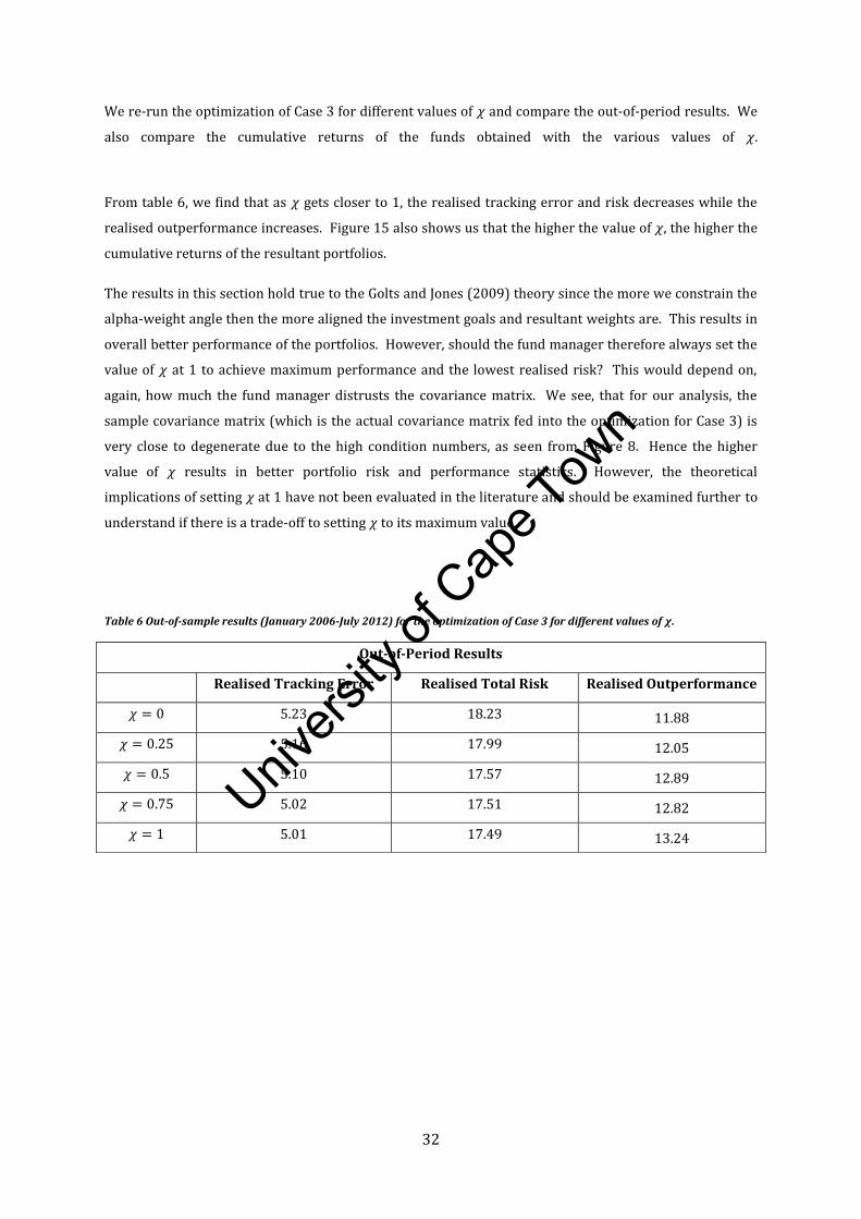
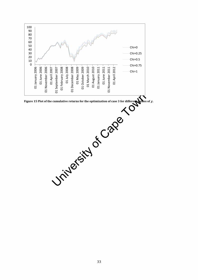
We re-run the optimization of Case 3 for different values of and compare the out-of-period results. We
also compare the cumulative returns of the funds obtained with the various values of
From table 6, we find that as gets closer to 1, the realised tracking error and risk decreases while the
realised outperformance increases. Figure 15 also shows us that the higher the value of , the higher the
cumulative returns of the resultant portfolios.
The results in this section hold true to the Golts and Jones (2009) theory since the more we constrain the
alpha-weight angle then the more aligned the investment goals and resultant weights are. This results in
overall better performance of the portfolios. However, should the fund manager therefore always set the
value of at 1 to achieve maximum performance and the lowest realised risk? This would depend on,
again, how much the fund manager distrusts the covariance matrix. We see, that for our analysis, the
sample covariance matrix (which is the actual covariance matrix fed into the optimization for Case 3) is
very close to degenerate due to the high condition numbers, as seen from Figure 8. Hence the higher
value of results in better portfolio risk and performance statistics. However, the theoretical
implications of setting at 1 have not been evaluated in the literature and should be examined further to
understand if there is a trade-off to setting to its maximum value .
Table 6 Out-of-sample results (January 2006-July 2012) for the optimization of Case 3 for different values of .
Out-of-Period Results
Realised Tracking Error Realised Total Risk Realised Outperformance
5.23 18.23 11.88
5.16 17.99 12.05
5.10 17.57 12.89
5.02 17.51 12.82
5.01 17.49 13.24
Univers
ity of
Cap
e Tow
n
33
Figure 15 Plot of the cumulative returns for the optimization of case 3 for different values of .
0 10 20 30 40 50 60 70 80 90
100
01
Jan
uar
y 2
00
6
01
Ju
ne
20
06
01
No
vem
ber
20
06
01
Ap
ril 2
00
7
01
Sep
tem
ber
20
07
01
Feb
ruar
y 2
00
8
01
Ju
ly 2
00
8
01
Dec
emb
er 2
00
8
01
May
20
09
01
Oct
ob
er 2
00
9
01
Mar
ch 2
01
0
01
Au
gust
20
10
01
Jan
uar
y 2
01
1
01
Ju
ne
20
11
01
No
vem
ber
20
11
01
Ap
ril 2
01
2
Chi=0
Chi=0.25
Chi=0.5
Chi=0.75
Chi=1
Univers
ity of
Cap
e Tow
n
34
8 Conclusion
The dissertation above has hopefully provided a new and exciting approach to portfolio optimization. We
have explored the shortfalls of the standard Markowitz theory with particular focus on the effect of
estimation error on the optimization. We then built on the theory of Golts and Jones (2009) which
combats this issue by imposing a more robust optimization technique.
In our empirical application of the technique, we have illustrated a definite improvement in the straight-
forward Markowitz theory as well as optimization using the shrinkage estimator. Our backtesting results
indicate that the portfolios constructed using Golts and Jones (2009) robust optimization outperformed
those constructed using traditional Markowitz covariance matrix and a shrunk-to-average covariance
matrix due to the method’s ability to align the investment goals with the optimized weights. Our results
also showed that the Golts and Jones (2009) method produces a covariance matrix with is better
conditioned, therefore, resulting in portfolios with lower out-of-sample risk and tracking error. We found
that the performance statistics such as the Sharpe Ratio and Information Ratio were the highest for the
portfolios constructed using the Golts and Jones (2009) robust optimization method. Finally, we showed
that the Golts and Jones (2009) method produces funds which have lower concentration.
We have used the research of Golts and Jones (2009) as a basis to show how the combination of Bayesian
methods and a geometric view on the portfolio selection problem provides a new outlook on the topic.
The idea of aligning the expected returns and weights opens up new opportunities of research for the
field. Quasi convex optimization and other topics in non-linear optimization may also prove to be
valuable additions to the literature to assist in constraining the Golts and Jones’ alpha-weight angle. Our
hope for the future is to apply methods such as these to build on the concepts introduced in this project.
Univers
ity of
Cap
e Tow
n
35
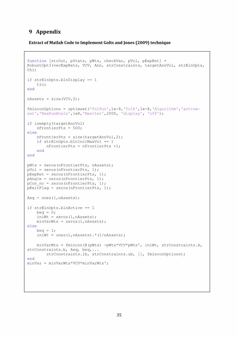
9 Appendix
Extract of Matlab Code to Implement Golts and Jones (2009) technique
function [strOut, pStats, pWts, checkVar, pVol, pExpRet] =
RobustOpt3(vecExpRets, VCV, Ann, strConstraints, targetAnnVol, strBlnOpts,
Chi)
if strBlnOpts.blnDisplay == 1 tic; end
nAssets = size(VCV,2);
fminconOptions = optimset('TolFun',1e-8,'TolX',1e-8,'Algorithm','active-
set','MaxFunEvals',1e8,'MaxIter',2000, 'display', 'off');
if isempty(targetAnnVol) nFrontierPts = 500; else nFrontierPts = size(targetAnnVol,2); if strBlnOpts.blnInclMaxVol == 1 nFrontierPts = nFrontierPts +1; end end
pWts = zeros(nFrontierPts, nAssets); pVol = zeros(nFrontierPts, 1); pExpRet = zeros(nFrontierPts, 1); pAngle = zeros(nFrontierPts, 1); pCon_no = zeros(nFrontierPts, 1); pExitFlag = zeros(nFrontierPts, 1);
Aeq = ones(1,nAssets);
if strBlnOpts.blnActive == 1 beq = 0; iniWt = zeros(1,nAssets); minVarWts = zeros(1,nAssets); else beq = 1; iniWt = ones(1,nAssets).*(1/nAssets);
minVarWts = fmincon(@(pWts) -pWts*VCV*pWts', iniWt, strConstraints.A,
strConstraints.b, Aeq, beq,... strConstraints.lb, strConstraints.ub, [], fminconOptions); end minVar = minVarWts*VCV*minVarWts';
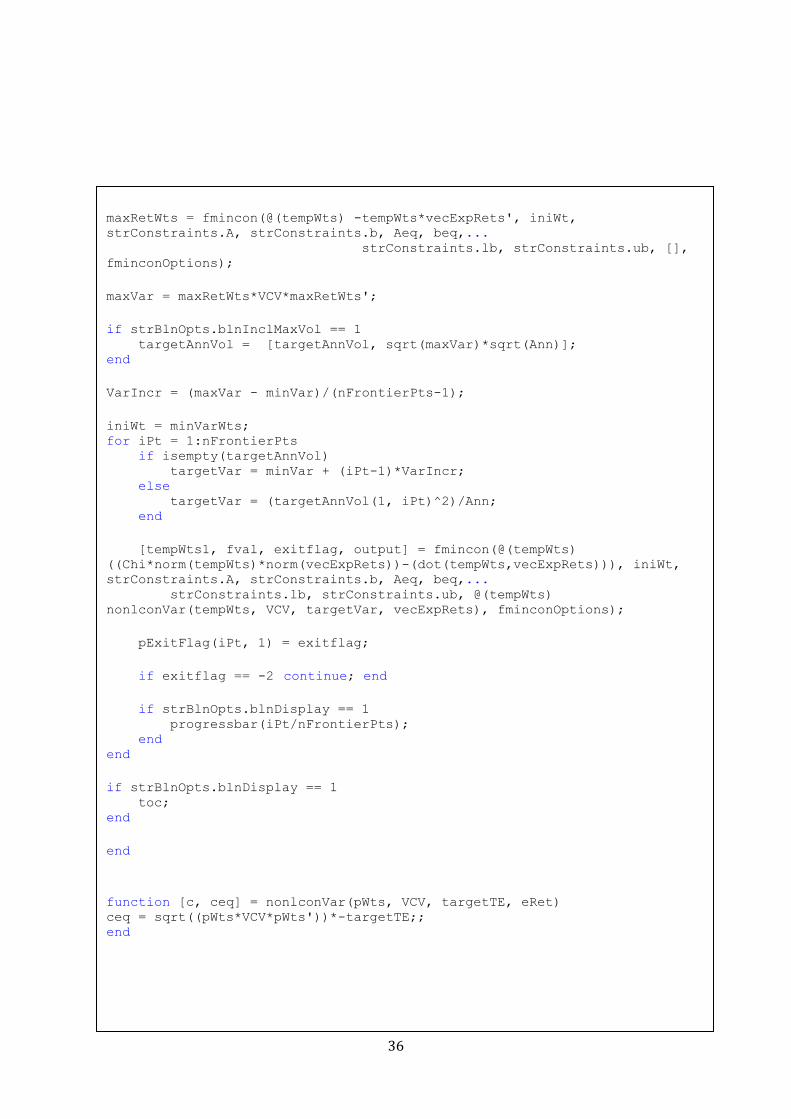
Univers
ity of
Cap
e Tow
n
36
maxRetWts = fmincon(@(tempWts) -tempWts*vecExpRets', iniWt,
strConstraints.A, strConstraints.b, Aeq, beq,... strConstraints.lb, strConstraints.ub, [],
fminconOptions);
maxVar = maxRetWts*VCV*maxRetWts';
if strBlnOpts.blnInclMaxVol == 1 targetAnnVol = [targetAnnVol, sqrt(maxVar)*sqrt(Ann)]; end
VarIncr = (maxVar - minVar)/(nFrontierPts-1);
iniWt = minVarWts; for iPt = 1:nFrontierPts if isempty(targetAnnVol) targetVar = minVar + (iPt-1)*VarIncr; else targetVar = (targetAnnVol(1, iPt)^2)/Ann; end
[tempWts1, fval, exitflag, output] = fmincon(@(tempWts)
((Chi*norm(tempWts)*norm(vecExpRets))-(dot(tempWts,vecExpRets))), iniWt,
strConstraints.A, strConstraints.b, Aeq, beq,... strConstraints.lb, strConstraints.ub, @(tempWts)
nonlconVar(tempWts, VCV, targetVar, vecExpRets), fminconOptions);
pExitFlag(iPt, 1) = exitflag;
if exitflag == -2 continue; end
if strBlnOpts.blnDisplay == 1 progressbar(iPt/nFrontierPts); end end
if strBlnOpts.blnDisplay == 1 toc; end
end
function [c, ceq] = nonlconVar(pWts, VCV, targetTE, eRet) ceq = sqrt((pWts*VCV*pWts'))*-targetTE;;
end
Univers
ity of
Cap
e Tow
n
37
10 Bibliography
Black, F., & Litterman, R. (1992). Global Portfolio Optimization. Financial Analysts Journal , 28.
Brown, S. (1976). Optimal Portfolio Choice Under Uncertainty: A Bayesian Approach. Phd
Dissertation, Univeristy of Chicago.
Brown, S. (1978). The portfolio choice problem: comparison of certainty equivalence and
optimal Bayes Portfolios. Communications in Statistics - Simulation and Computation , 321-334.
Chopra, V., & Ziemba, W. (1993). The effect of errors in means, variance and covariance on
optimal portfolio selection. Journal of Portfolio Management , 6-11.
Fama, E., & French, K. (1993). Common Risk Factors in the Returns on Stocks and Bonds. Journal
of Financial Economics , 3-56.
Frankfurter, G., Phillips, H., & Seagle, J. (1971). Portfolio selection: The effect of uncertain means,
variances and covariances. Journal of Financial and Quantitative Analysis , 1251-1262.
Frost, P., & Savarino, J. (1986). An empirical Bayes approach to efficient portfolio selection.
Journal of Financial and Quantitative Analysis , 293-305.
Goldfarb, D., & Iyengar, G. (2003). Robust Portfolio Selection Problems. Mathematics of
operations research, Vol 28, No. 1 , 1-38.
Golts, M., & Jones, G. (2009, October 5). A sharper angle on portfolio optimization. Retrieved June
2012, from SSRN: http://ssrn.com/abstract=1483412
Jobson, J., & Korkie, B. (1980). Estimation for Markowitz Efficient Portfolios. Journal of the
American Statistical Association , 544-554.
Jorian, P. (1986). Bayes-Stein Estimation for Portfolio Analysis. The Journal of Financial and
Quantitative Analysis, Vol 21 No. 3 , 279-292.
Jorian, P. (1992). Portfolio Optimization in Practice. Financial Analysts Journal, Vol. 48, No.1 , 68-
74.
Kan , R., & Zhou, G. (2007). Optimal portfolio choice with parameter uncertainty. Journal of
Financial and Quantitative Analysis , 621-656.
Kgomari, W., & Bradfield, D. (2004). Concentration - Should we be mindful of it? Cadiz Financial
Strategists, Quantitative Research.
Lai, T., Xing, H., & Chen, Z. (2009). Mean-variance portfolio optimization when means and
covariances are unknown. Stanford: Department of Statistics, Stanford Univerisity.
Univers
ity of
Cap
e Tow
n
38
Ledoit, O., & Wolf, M. (2004). A well-conditioned estimator for large dimensional covariance
matrices. Journal of Multivariate Analysis, Vol 88 , 65-411.
Ledoit, O., & Wolf, M. (2004). A Well-Conditioned Estimator for Large-Dimensional Covariance
Matrices. Journal of Multivariate Analysis , 365-411.
Ledoit, O., & Wolf, M. (2003). Honey, I Shrunk the Sample Covariance Matrix. Problems. Journal
of Portfolio Management, vol 30 , 110-119.
Ledoit, O., & Wolf, M. (2001). Improved Estimation of the Covariance Matrix of Stock Returns
With an Application to Portfolio Selection. Journal of Empirical Finance , 603-621.
Markowitz, H. (1952). Portfolio Selection. The Journal of Finance , 77-91.
Markowitz, H. (1959). Portfolio Selection: Efficient Diversification of Investments. Wiley, Yale
University Press.
Menchero, J., Wang, J., & Orr, D. (2012). Improving risk forecasts for optimized portfolios.
Financial Analysts Journal, Vol 68, No.3 , 40-49.
Merton, R. (1980). On estimating the expected return on the market : An exploratory
investigation. Journal of Financial Economics, Vol 8 (4) , 323-361.
Meucci, A. (2011, May 12). Robust Bayesian Allocation. Retrieved November 2012, from
Symmys: http://symmys.com/node/102
Michaud, R. O. (1989). The Markowitz optimization enigma: Is 'Optimized' optimal? Financial
Analysts Journal, Vol 45, No. 1 , 31-42.
Munro, B. (2010). Covariance estimation for South African Equity portfolios. Cape Town: Cadiz
Securities.
Phillippe. (2013). Quantitative Finance. Retrieved January 23, 2013, from Stack Exchange:
www.quant.stackexchange.com/questions/7080/robust-bayesian-optimization-in-markowitz-
framework
Scherer, B. (2007). Portfolio Construction and Risk Budgeting, 3rd Edition. Risk Books.
Stein, C. (1955). Inadmissibility of the Usual Estimator for the Mean of a Multivariate
Distribution. Proceedings of the Third Berkeley Symposium , 197-206.
Stubbs, R. A., & Ceria, S. (2006, May). Incorporating estimation errors into portfolio selection:
robust portfolio construction. Retrieved November 2012, from Axioma: www.axiomainc.com
Tutuncu, R., & Koenig, M. (2004). Robust Asset Allocation. Annals of Operations Research Vol. 132
, 157-187.
Zimmermann, H., & Nierdermayer, D. (2007, November). Robust Portfolio Optimization.


