
RESPONSE SPECTRUM OF LINEAR ELASTIC SYSTEM
FOR 2001 BHUJ EARTHQUAKE
Bhumika B. Mehta M. E. CIVIL – CASAD.
B-2, Kalindi Flats, Opp. Kadwa Patidar Boarding, C. G. Road, Ahmedabad – 380 006
Ph. No. – (079) 6561093 [email protected]
PDF created with FinePrint pdfFactory trial version http://www.fineprint.com

CONTENTS
1. CONCEPT OF RESPONSE SPECTRUM
2. RESPONSE QUANTITIES
3. NUMERICAL EVALUATION OF RESPONSE SPECTRUM
4. DEFORMATION, VELOCITY AND ACCELERATION RESPONSE
SPECTRUM
4.1 Deformation response spectrum
4.2 Pseudo velocity response spectrum
4.3 Pseudo velocity response spectrum
4.4 True/Relative velocity response spectrum
4.5 True/Relative acceleration response spectrum
5. PROCEDURE TO CONSTRUCT RESPONSE SPECTRUM OF THE
EARTHQUAKE
6. PEAK STRUCTURAL RESPONSE FROM THE RESPONSE
SPECTRUM
7. TRIPARTITE RESPONSE SPECTRUM
7.1 Procedure to construct tripartite plot
8. FACTORS AFFECTING RESPONSE SPECTRUM
9. RESPONSE SPECTRUM CHARACTERISTICS
10. APPLICATIONS OF RESPONSE SPECTRUM
11. DESIGN SPECTRUM
11.1 Procedure to construct design spectrum
PDF created with FinePrint pdfFactory trial version http://www.fineprint.com

RESPONSE SPECTRUM OF LINEAR ELASTIC
SYSTEM FOR 2001 BHUJ EARTHQUAKE
One of the central problem of engineering seismology is the calculation of the
behaviour of a structure subjected to a given ground motion. An exact solution of this
problem in transient dynamics is rarely possible because of the great complexity of the
ground motions associated with earthquakes, and because of the complicated nature of
many of the structures of interest to the engineer. One of the attempts to simplify this
problem has involved the introduction of the “ response spectrum”.
1. CONCEPT OF RESPONSE SPECTRUM
Response spectrum of any earthquake ground motion is simply a plot of the
maximum response during that earthquake of a single degree of freedom (SDF)
system as a function of its natural vibration period Tn or frequency (ωn or fn), for a
given value of damping. Maximum response may be displacement, velocity or
acceleration. Each such plot has a fixed damping ratio ξ, and several such plots for
different values of ξ are included to cover the range of damping values encountered in
actual structures.
Now a central concept in earthquake engineering, the response spectrum
provides a convenient means to summarize the peak response of all possible linear
single degree of freedom systems to a particular component of earthquake ground
motion.
2. RESPONSE QUANTITIES
As a structural engineer, mostly we concerned with the deformation of the
structural system or displacement u(t) of the mass relative to the moving ground, to
which the internal forces are linearly varied.
This response quantity is deformation or displacement, velocity or
acceleration. These are the bending moments and shear forces in beams and columns
PDF created with FinePrint pdfFactory trial version http://www.fineprint.com
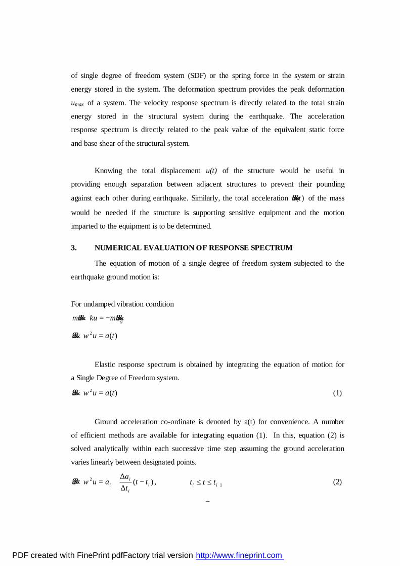
of single degree of freedom system (SDF) or the spring force in the system or strain
energy stored in the system. The deformation spectrum provides the peak deformation
umax of a system. The velocity response spectrum is directly related to the total strain
energy stored in the structural system during the earthquake. The acceleration
response spectrum is directly related to the peak value of the equivalent static force
and base shear of the structural system.
Knowing the total displacement u(t) of the structure would be useful in
providing enough separation between adjacent structures to prevent their pounding
against each other during earthquake. Similarly, the total acceleration )(tu&& of the mass
would be needed if the structure is supporting sensitive equipment and the motion
imparted to the equipment is to be determined.
3. NUMERICAL EVALUATION OF RESPONSE SPECTRUM
The equation of motion of a single degree of freedom system subjected to the
earthquake ground motion is:
For undamped vibration condition
gumkuum &&&& −=+
)(2 tauu =+ ω&&
Elastic response spectrum is obtained by integrating the equation of motion for
a Single Degree of Freedom system.
)(2 tauu =+ ω&& (1)
Ground acceleration co-ordinate is denoted by a(t) for convenience. A number
of efficient methods are available for integrating equation (1). In this, equation (2) is
solved analytically within each successive time step assuming the ground acceleration
varies linearly between designated points.
)(2i
i
ii tt
t
aauu −
∆∆
+=+ ω&& , 1+≤≤ ii ttt (2)
PDF created with FinePrint pdfFactory trial version http://www.fineprint.com
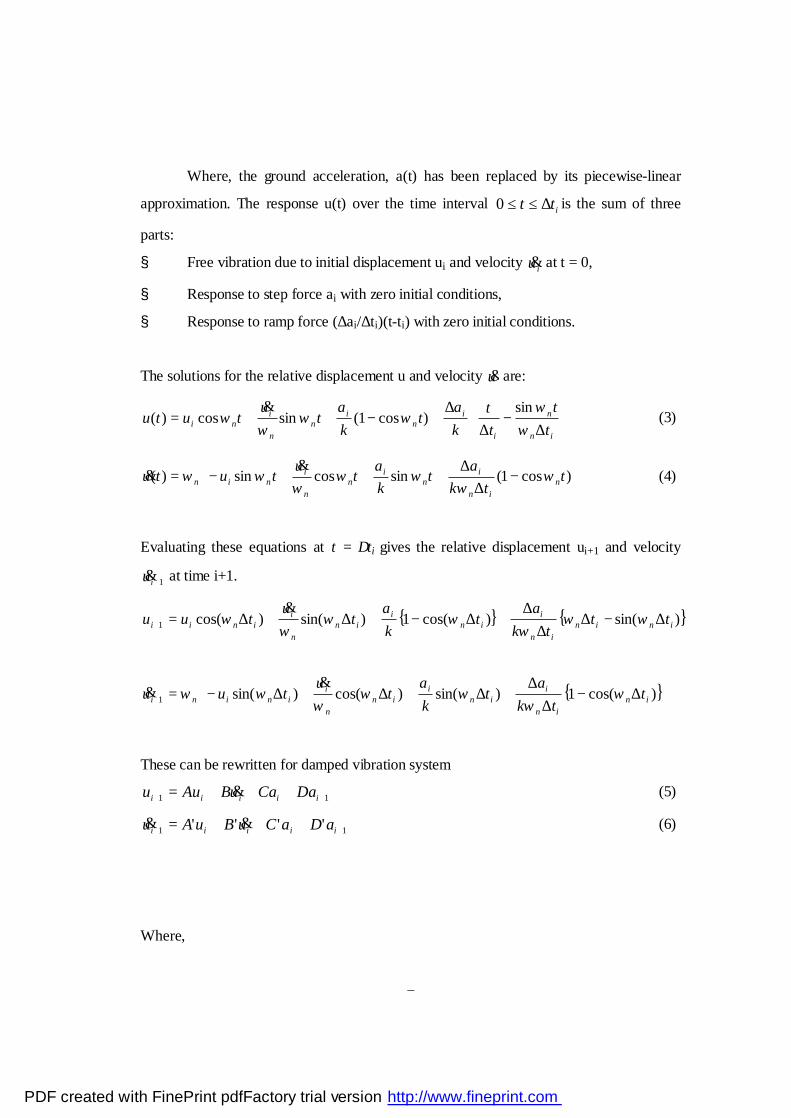
Where, the ground acceleration, a(t) has been replaced by its piecewise-linear
approximation. The response u(t) over the time interval itt ∆≤≤0 is the sum of three
parts:
§ Free vibration due to initial displacement ui and velocity iu& at t = 0,
§ Response to step force ai with zero initial conditions,
§ Response to ramp force (∆ai/∆ti)(t-ti) with zero initial conditions.
The solutions for the relative displacement u and velocity u& are:
∆
−∆
∆+−++=
in
n
i
in
in
n
ini t
t
t
t
k
at
k
at
ututu
ωω
ωωω
ωsin
)cos1(sincos)(&
(3)
−
∆∆
+++−= )cos1(sincossin)( ttk
at
k
at
ututu n
in
in
in
n
inin ω
ωωω
ωωω
&& (4)
Evaluating these equations at t = ∆ti gives the relative displacement ui+1 and velocity
1+iu& at time i+1.
{ } { })sin()cos(1)sin()cos(1 ininin
iin
iin
n
iinii tt
tk
at
k
at
utuu ∆−∆
∆∆
+∆−+∆+∆=+ ωωω
ωωω
ω&
{ }
∆−
∆∆
+∆+∆+∆−=+ )cos(1)sin()cos()sin(1 inin
iin
iin
n
iinini t
tk
at
k
at
utuu ω
ωωω
ωωω
&&
These can be rewritten for damped vibration system
11 ++ +++= iiiii DaCauBAuu & (5)
11 '''' ++ +++= iiiii aDaCuBuAu && (6)
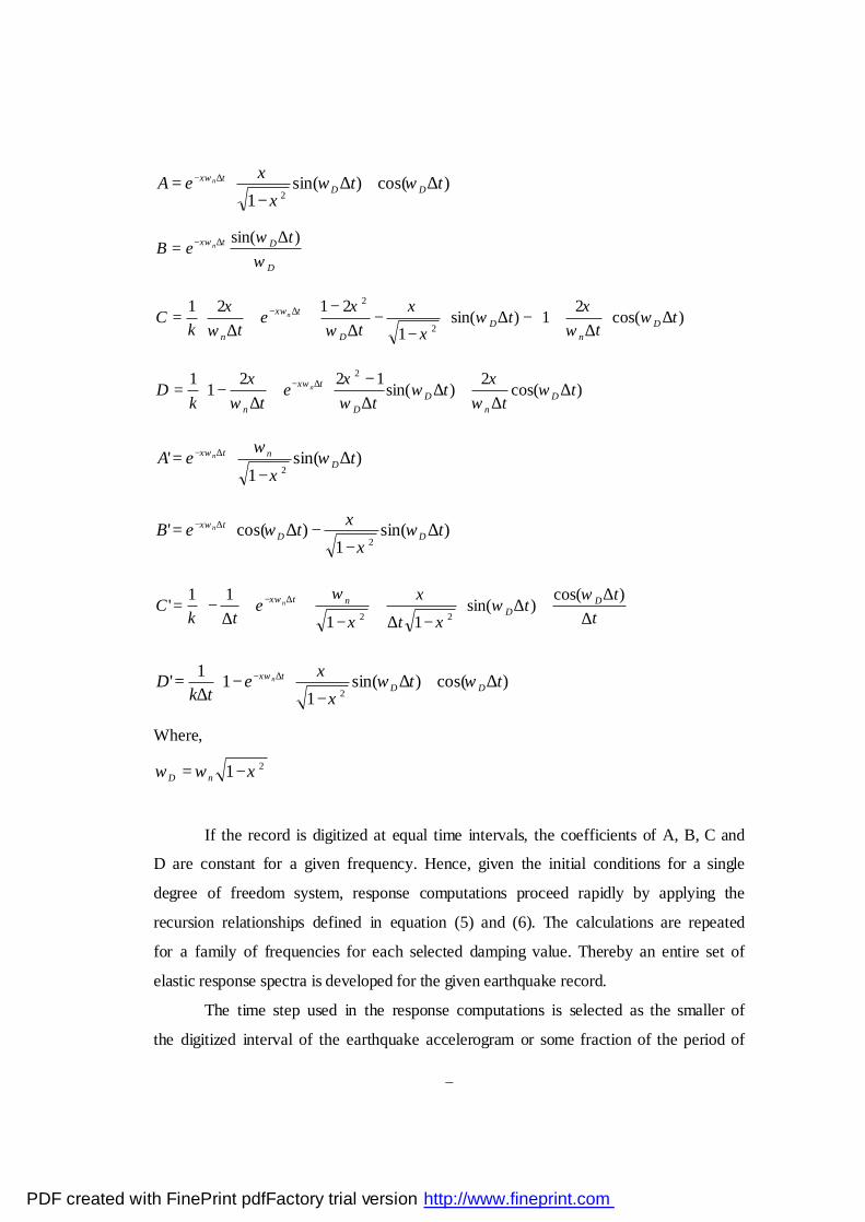
Where,
PDF created with FinePrint pdfFactory trial version http://www.fineprint.com
∆+∆
−= ∆− )cos()sin(
1 2tteA DD
tn ωωξ
ξξω
D
Dt teB n
ωωξω )sin( ∆
= ∆−
∆
∆
+−∆
−−
∆−
+∆
= ∆− )cos(2
1)sin(1
21212
2
tt
tt
etk
C Dn
DD
t
n
n ωω
ξω
ξ
ξω
ξω
ξ ξω
∆
∆+∆
∆−
+∆
−= ∆− )cos(2
)sin(122
11 2
tt
tt
etk
D Dn
DD
t
n
n ωω
ξω
ωξ
ωξ ξω
∆
−= ∆− )sin(
1'
2teA D
ntn ωξ
ωξω
∆
−−∆= ∆− )sin(
1)cos('
2tteB DD
tn ωξ
ξωξω
∆∆
+∆
−∆+
−+
∆−= ∆−
t
tt
te
tkC D
Dntn
)cos()sin(
11
11'
22
ωω
ξ
ξ
ξ
ωξω
∆+∆
−−
∆= ∆− )cos()sin(
11
1'
2tte
tkD DD
tn ωωξ
ξξω
Where,
21 ξωω −= nD
If the record is digitized at equal time intervals, the coefficients of A, B, C and
D are constant for a given frequency. Hence, given the initial conditions for a single
degree of freedom system, response computations proceed rapidly by applying the
recursion relationships defined in equation (5) and (6). The calculations are repeated
for a family of frequencies for each selected damping value. Thereby an entire set of
elastic response spectra is developed for the given earthquake record.
The time step used in the response computations is selected as the smaller of
the digitized interval of the earthquake accelerogram or some fraction of the period of
PDF created with FinePrint pdfFactory trial version http://www.fineprint.com

free vibration, for example T/10. For systems whose natural period governs the
selection of ∆ti, i.e. for high frequencies, ∆ti must be chosen so that an integral number
of time steps comprise the digitized interval of the accelerogram. This restriction on
∆ti preserves uniform time intervals and guarantees that response quantities will be
computed at times corresponding to those of the given earthquake record.
4. DEFORMATION, VELOCITY AND ACCELERATION RESPONSE
SPECTRUM
4.1 Deformation response spectrum
Deformation response spectrum is a plot of the maximum displacement that a
SDF structure is experienced during the earthquake as a function of its natural
vibration period for a given value of damping.
The deformation response spectrum provides all the necessary information to
compute peak values of deformation SD = umax and internal forces. Here the spectrum
is developed for a longitudinal component of Bhuj earthquake of 2001 at station
Ahmedabad. For each system the peak value is of deformation SD = umax is
determined from the deformation history. Usually the peak occurs during ground
shaking, however, for lightly damped systems with very long natural periods the peak
response may occur during the free vibration phase after the ground shaking has
stopped. The spectrum is complete when all possible values of damping are plotted.
The peak deformation SD = 46.917mm for Tn = 1 sec and ξ = 5%.
The peak deformation SD = 98.516mm for Tn = 5 sec and ξ = 5%.
The peak deformation SD = 237.346mm for Tn = 10 sec and ξ = 5%.
The peak deformation SD = 117.900mm for Tn = 15 sec and ξ = 5%.
PDF created with FinePrint pdfFactory trial version http://www.fineprint.com

Figure 1
N 78 E Component of Bhuj Earthquake
Tn = 1 sec
ξ = 5%
PDF created with FinePrint pdfFactory trial version http://www.fineprint.com

Tn = 5 sec
ξ = 5%
Tn = 10 sec
ξ = 5%
Tn = 15 sec
ξ = 5%
Figure 2
Deformation Response of Four SDOF Systems
PDF created with FinePrint pdfFactory trial version http://www.fineprint.com

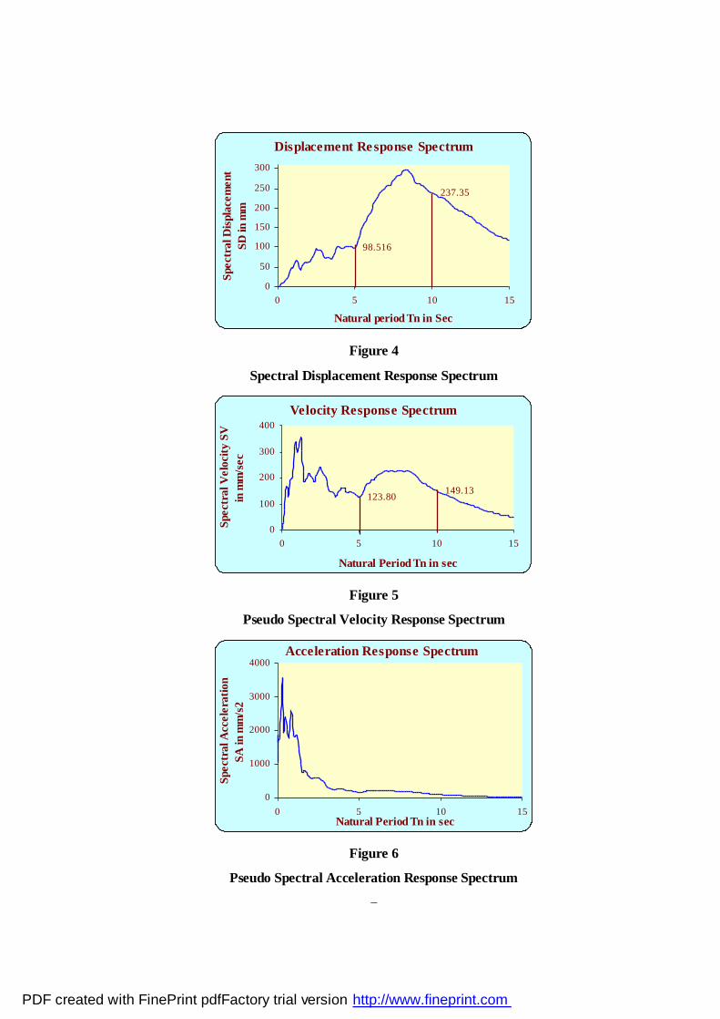
Displacement Response Spectrum
237.35
98.516
117.9
0
50
100
150
200
250
300
0 2 4 6 8 10 12 14
Natural period Tn in Sec
Sp
ectr
al D
isp
lace
men
t S
D in
mm
Figure 3
Displacement Response Spectrum for ξ = 5%
4.2 Pseudo velocity response spectrum
Pseudo velocity response spectrum is a plot of pseudo spectral velocity PSV
and natural period Tn that an SDF structure is experienced during the earthquake for a
given value of damping.
)(2
)(ω SDT
SDPSVn
nπ==
PSV is pseudo spectral velocity. It is pseudo because it is not velocity but it has
units of velocity. It is related to the peak value of strain energy Emax stored in the SDF
system during the earthquake.
2222maxmax )(
2
1)(
2
1)(
2
1
2
1PSVmSDmSDkkuE ==== ω
The peak pseudo spectral velocity PSV for a system with natural period Tn and
spectral displacement SD can be determined from the equation.
For Tn = 1 sec, ξ = 5% and D = 46.917 mm, PSV = 294.79 mm/sec.
PDF created with FinePrint pdfFactory trial version http://www.fineprint.com
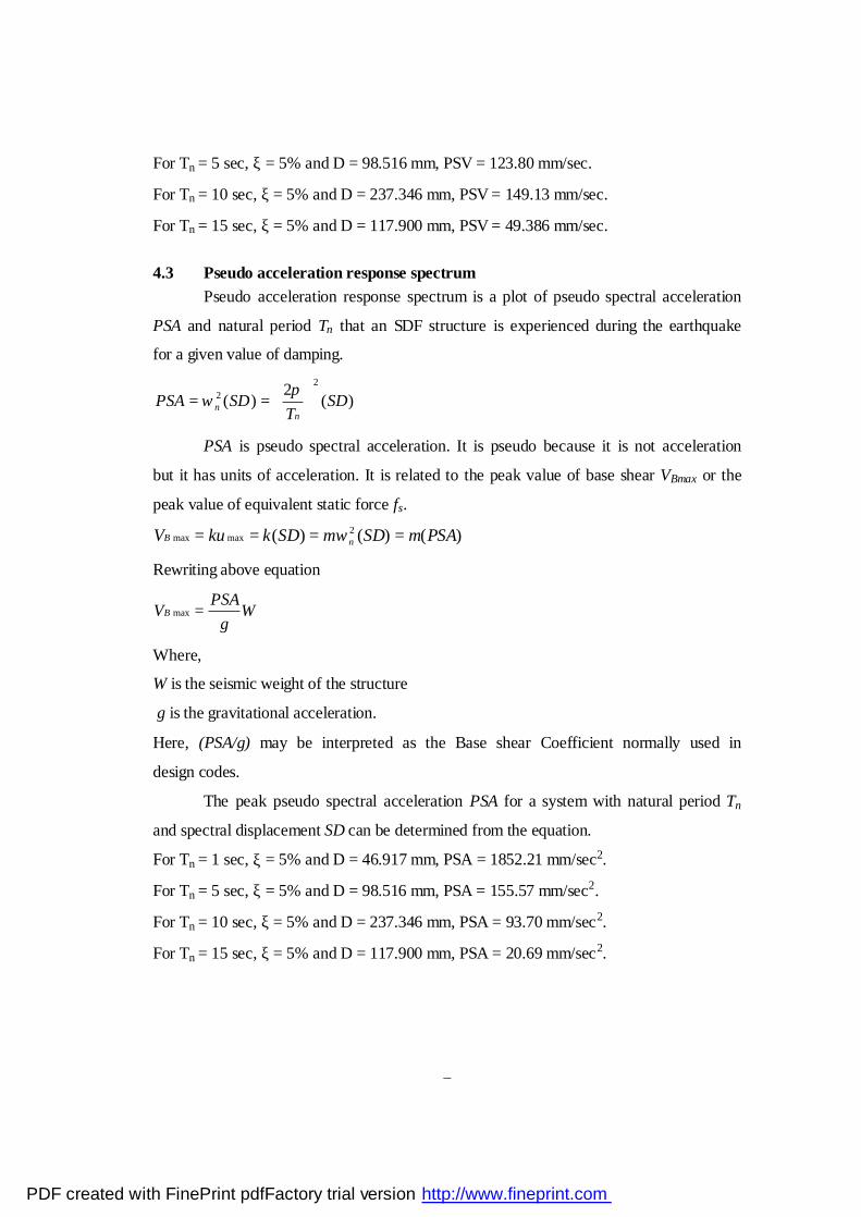
For Tn = 5 sec, ξ = 5% and D = 98.516 mm, PSV = 123.80 mm/sec.
For Tn = 10 sec, ξ = 5% and D = 237.346 mm, PSV = 149.13 mm/sec.
For Tn = 15 sec, ξ = 5% and D = 117.900 mm, PSV = 49.386 mm/sec.
4.3 Pseudo acceleration response spectrum
Pseudo acceleration response spectrum is a plot of pseudo spectral acceleration
PSA and natural period Tn that an SDF structure is experienced during the earthquake
for a given value of damping.
)(2
)(2
2 SDT
SDPSAn
n
==
πω
PSA is pseudo spectral acceleration. It is pseudo because it is not acceleration
but it has units of acceleration. It is related to the peak value of base shear VBmax or the
peak value of equivalent static force fs.
)()()( 2maxmax PSAmSDmSDkkuV nB ==== ω
Rewriting above equation
Wg
PSAVB =max
Where,
W is the seismic weight of the structure
g is the gravitational acceleration.
Here, (PSA/g) may be interpreted as the Base shear Coefficient normally used in
design codes.
The peak pseudo spectral acceleration PSA for a system with natural period Tn
and spectral displacement SD can be determined from the equation.
For Tn = 1 sec, ξ = 5% and D = 46.917 mm, PSA = 1852.21 mm/sec2.
For Tn = 5 sec, ξ = 5% and D = 98.516 mm, PSA = 155.57 mm/sec2.
For Tn = 10 sec, ξ = 5% and D = 237.346 mm, PSA = 93.70 mm/sec2.
For Tn = 15 sec, ξ = 5% and D = 117.900 mm, PSA = 20.69 mm/sec2.
PDF created with FinePrint pdfFactory trial version http://www.fineprint.com
Displacement Response Spectrum
237.35
98.516
0
50
100
150
200
250
300
0 5 10 15
Natural period Tn in Sec
Spec
tral
Dis
plac
emen
t SD
in m
m
Figure 4
Spectral Displacement Response Spectrum
Velocity Response Spectrum
123.80149.13
0
100
200
300
400
0 5 10 15
Natural Period Tn in sec
Spec
tral
Vel
ocit
y SV
in
mm
/sec
Figure 5
Pseudo Spectral Velocity Response Spectrum
Acceleration Response Spectrum
0
1000
2000
3000
4000
0 5 10 15Natural Period Tn in sec
Spec
tral
Acc
eler
atio
n SA
in m
m/s
2
Figure 6
Pseudo Spectral Acceleration Response Spectrum
PDF created with FinePrint pdfFactory trial version http://www.fineprint.com

4.4 True/Relative velocity response spectrum
The true or relative velocity response spectrum )(tu& can be determined from
the equation (6) of section 3. The difference between relative velocity spectra and
pseudo velocity spectra depend on the natural period of the system. For long period
systems, PSV is less than maxu& and differences between the two are large. This can be
understood by recognizing that as Tn becomes very long, the mass of the system stays
still while the ground underneath moves. For short period systems PSV exceeds maxu& ,
with the differences increasing as Tn becomes shorter. For medium period systems, the
differences between PSV and maxu& are small over a wide range of Tn.
Velocity Response Spectrum
0
50
100
150
200
250
300
350
400
0 5 10 15
Natural Period Tn in sec
Sp
ectr
al V
eloc
ity
SV
in m
m/s
ec
Pseudo velocity
Relative velocity
Figure 7
Comparison of True and Pseudo Velocity Response Spectrum
4.5 True/Relative acceleration response spectrum
The true or relative acceleration response spectrum )(tu&& can be determined
from the following equation.
)(2)()( 2 tututu nn&&& ξωω += (7)
Where,
u(t) = Spectral Displacement
PDF created with FinePrint pdfFactory trial version http://www.fineprint.com

)(tu& = Relative velocity
The pseudo acceleration and relative acceleration response spectra are identical
for systems without damping. This is clear from equation (7).
PSAtutu n == )()( 2ω&&
For systems with damping, it is possible only when )(tu& = 0. In this case u(t)
attains its peak umax. at this instant )(2 tunω represent the true acceleration of the mass.
Equation (7) suggests that the differences between PSA and )(tu&& are expected to
increases as the damping increases.
The difference between two spectra is small for short period systems and is of
some significance only for long period systems with large values of damping. As the
natural period Tn of a system approaches infinity, the mass of the system stays still
while the ground moves. Thus deformation reaches to peak ground displacement and
PSA reaches zero.
Acceleration Response Spectrum
0
500
1000
1500
2000
2500
3000
3500
4000
0 5 10 15
Natural Period Tn in sec
Sp
ectr
al A
ccel
erat
ion
SA
in m
m/s
2
Pseudo acceleration
Relat ive acceleration
Figure 8
Comparison of True and Pseudo Acceleration Response Spectrum
PDF created with FinePrint pdfFactory trial version http://www.fineprint.com

5. PROCEDURE TO CONSTRUCT RESPONSE SPECTRUM OF THE
EARTHQUAKE
a) Take the ground motion data of an earthquake. This ground acceleration data
gu&& is available from the accelerogram, which is earthquake-measuring
instrument. This ground motion ordinates are defined at suitable interval.
Generally it is at 0.02 sec.
b) For the particular value of damping ξ take the different value of natural period
Tn of a single degree of freedom system (SDF).
c) Compute the deformation response u(t) of this SDF system due to the ground
motion )(tug&& by method developed in section 3.
d) Determine umax, the peak value of u(t).
e) The spectral ordinates are SD = umax, PSV = (2π/Tn)SD and PSA = (2π/Tn)2
SD. here SD is spectral displacement, PSV is pseudo spectral velocity and PSA
is pseudo spectral acceleration.
f) Repeat above steps except first for a different range of Tn and ξ values
covering all possible systems of engineering interest.
g) Draw the results graphically to produce three separate spectra.
h) Above all figure shows the graphical representation of construction of
displacement response spectrum, velocity response spectrum and acceleration
response spectrum of Bhuj earthquake of 2001 at station Ahmedabad.
6. PEAK STRUCTURAL RESPONSE FROM THE RESPONSE
SPECTRUM
If the response spectrum for a given ground motion component is available, the
peak value of deformation or of an internal force in any linear SDF system can be
determined readily. Corresponding to the natural vibration period Tn and damping
ratio ξ of the system, the values of SD, PSV, PSA are read from the spectrum. Now all
response quantities of interest can be expressed in terms of SD, PSV, PSA and the
mass or stiffness properties of the system. The peak deformation of the system is
PDF created with FinePrint pdfFactory trial version http://www.fineprint.com

PSAT
PSVT
SDunn
2
max22
===
ππ
And the peak value of the equivalent static force fsmax is
)(maxmax PSAmkufs ==
Static analysis of the one story frame subjected to lateral force fsmax provides the
internal forces (e.g. shear force s and bending moments in columns and beams). The
peak values of shear force and bending moment at the base of the one story structure
are:
)(maxmax PSAmkuVB ==
maxmax BB hVM =
h
fsmax
VBmax
MBmax
Figure 9
Peak Value of Equivalent Static Force
Only one of the three spectra – deformation, pseudo velocity and pseudo
acceleration is sufficient for computing the peak deformations and forces required in
structural design.
7. TRIPARTITE RESPONSE SPECTRUM
Each of the three spectra, SD, PSV and PSA, give exactly the same
information. No new information is given by any one of them. The three spectra are
simply different ways of presenting the same information on structural response. From
one of them we can get the other spectra. Usually, these spectra are together drawn on
a single log plot.
PDF created with FinePrint pdfFactory trial version http://www.fineprint.com

If all the three spectra provide same information than why do we need three
different spectra and what can be obtained from any one of the other two? One of the
reasons is that each spectrum directly provides a physically meaningful quantity. The
deformation response spectrum provides the peak deformation or displacement of a
system. The pseudo velocity response spectrum is directly related to the peak strain
energy stored in the system during the earthquake. The pseudo acceleration response
spectrum is directly related to the peak value of the equivalent static force and base
shear. The second reason is the shape of the spectrum can be approximated more
readily for design purposes with the support of all three spectral quantities rather than
any one of them alone (elastic design spectrum)
The three spectral quantities are interrelated by relation
)(SDPSVPSA
n
n
ωω
==
SDT
PSVPSAT
n
n ππ
2
2==
The 4-way plot is a compact representation of the three – displacement, pseudo
velocity and pseudo acceleration response spectra. A response spectrum should cover
wide range of natural vibration periods and several damping values so that it provides
peak response of all possible structures.
The response spectrum has proven so useful in earthquake engineering that
spectra for virtually all ground motions string enough to be of engineering interest are
now computed and published soon after they are recorded. Enough of them have been
obtained to give us a reasonable idea of the kind of the motion that is likely to occur in
future earthquakes, and how response spectra are affected by distance to the causative
fault, local soil conditions, and regional geology.
7.1 Procedure to construct tripartite plot
a) Y-axis is the log(PSV) and X – axis is the log(Tn).
b) Now relation between PSV, PSA and Tn is PSVPSATn
=π2
Taking log scale on both side
PDF created with FinePrint pdfFactory trial version http://www.fineprint.com

PSVPSATn log2logloglog =−+ π
now, log Tn = x, log PSV = y and log PSA is constant.
∴ π2loglog −+= PSAxy
∴y = x + constant
1=dx
dy
This is the equation of a straight line with slope = +1. the intercept on
Y – axis depends on PSA. Hence, constant PSA lines have a slope pf +1 means
they make an angle of +45° with X - axis.
c) Similarly, relation between PSV, SD and Tn is SDT
PSVn
π2=
Taking log scale on both sides
nTSDPSV loglog2loglog −+= π
Now, log Tn = x, log PSV = y and log SD is constant.
∴y = log 2π + log SD - x
∴y = -x + constant
1−=dx
dy
This represents a straight line with slope of – 1 means the constant SD
lines make an angle of -45° with X – axis.
d) Hence, SD and PSA values can be read in a log(PSV) versus log(T) plot on the
logarithmic scales oriented at 45° to the period scale. This 4-way plot is a
compact representation of the three response spectra.
PDF created with FinePrint pdfFactory trial version http://www.fineprint.com

1000
1000
0
SD mm
1000SA
mm
/sec2
0.1
0.001
0.01
0.01
10
1
SV
mm
/sec
100
100.1
10
0.001
0.01
Tn sec
0.1 1
0.0000
1
100
1000
1
0.0001
0.01
0.10.001
1000
10
100
1100
8
22.55
25.13
Figure 10
Combined D-V-A or Tripartite Plot
From the figure, for a pseudo spectral velocity PSV = 8 mm/sec and Tn = 2 sec,
PSA = 25.13 mm/sec2 and SD = 2.55 mm.
8. FACTORS AFFECTING RESPONSE SPECTRUM
The actual shape of the response spectrum is affected by
§ Fault length and size of shock,
§ Distance from fault
§ Local geology and geography.
For example, at large distances from fault, the high frequencies get filtered and
only low frequency waves spread. Thus, a site nearer to the fault will have more high
frequencies than farther ones. This is significant while designing structures. For
PDF created with FinePrint pdfFactory trial version http://www.fineprint.com

structures with high natural periods, a larger fault lying at greater distance from the
site may be critical, while for structures with low natural periods, a smaller fault lying
close to the structure may be more significant. This is also a reason why design
spectrum is at times arrived at by combining expected response spectra from different
faults for different frequency range.
9. RESPONSE SPECTRUM CHARACTERISITCS
For systems with very short natural period (stiff system), the peak pseudo
acceleration approaches maxgu&& and SD is very small. For example, a fixed mass and
very short period system is extremely stiff or essentially rigid. Such a system would be
expected to undergo very little deformation and its mass would move rigidly with the
ground; its peak acceleration should be approximately equal to maxgu&& and maximum
relative displacement SD and maximum relative velocity SV are small. Thus the
acceleration spectrum gives the maximum ground acceleration corresponding to the
acceleration value.
For systems with very long natural period (flexible system), the maximum
displacement approaches maxgu and pseudo acceleration is very small. Thus the forces
in the structure, which are related to m*PSA, would be very small. For example, a
fixed mass and very long period system is extremely flexible. In this type of system
mass would be expected to remain essentially stationary while the ground below
moves. Thus maximum relative displacement and maximum relative velocity
approaches maxgu and maxgu& . An increase in damping smoothens the spectrum curves
and lowers the average amplitude.
For intermediate systems with medium natural period, maximum velocity
approaches maxgu& . Over this period range, PSV may be idealized as constant at a value
equal to peak ground velocity.
PDF created with FinePrint pdfFactory trial version http://www.fineprint.com

Based on these observations response spectrum is divided into three parts with
low, medium and high natural periods. The long natural period region is called
displacement sensitive region. The short natural period region is called acceleration
sensitive region. And intermediate system having medium natural period is called
velocity sensitive region.
10. APPLICATIONS OF RESPONSE SPECTRUM
The use of the response spectrum has frequently been criticized of the grounds
that it is not possible to represent a complex structure by the very simplified model
containing only a single mass, spring and dashpot. It is important that it be clearly
understood that no exact equivalence between the response spectrum and the
behaviour of an actual structure is necessarily assumed nor implied in the response
spectrum technique. The practical usefulness of the response spectrum method is
based on the following consideration.
b) For complex structures in which system response must be calculated by
considering motions in a number of modes of vibration simultaneously, the
response spectrum may be used directly to get approximate solutions by the
principle of superposition. The response spectrum is concerned with maximum
values only, loses some information concerning the phases of the motions in
various modes. A superposition of the response values from the response
spectrum corresponding to the periods of the modes of vibration does,
however, give an approximate value of total system response. This
approximation is always on the safe side, since the assumption that the
maximum responses in the various modes will always occur at the same time,
will give a total value somewhat higher than the actual maximum response.
c) Many structures may, in spite of their complexity, behave under some
circumstances essentially as single degree of freedom systems, and for these
situations the response spectrum can be applied directly to give system
behaviour. Because of the way in which motion is excited, even very
complicated structures may move in essentially one mode of vibration. Ground
accelerations, for example, since they are equivalent to a distributed set of
PDF created with FinePrint pdfFactory trial version http://www.fineprint.com

inertia forces acting always in the same direction at all points in a structure,
tend to excite motion in which the fundamental mode of vibration
predominates.
d) A realistic evaluation of seismic coefficients or lateral force coefficients cannot
be obtained without the use of the response spectrum. The maximum
accelerations to be expected in a structure are not those which are recorded by
the ground motion accelerometer, since dynamic amplification effects can
occur which may take the structural accelerations considerably larger that the
ground accelerations. From the response spectrum, the maximum value of the
total base shear force is directly obtained.
e) The velocity spectrum gives directly the energy input into the system. By
equating this energy input to the sum of the various energy dissipation, which
occurs in the structure, a determination of overall system behaviour can be
made. Such energy methods, used in connection with a limit design technique,
will permit the establishment of rational dynamic strength criteria for many
structures subjected to earthquake loading.
f) Response spectrum gives the maximum response of a linear SDF system to a
given ground motion. Many real life structures can be idealized as single
degree of freedom systems. Hence, such structures can be directly analyzed
using the response spectrum.
11. DESIGN SPECTRUM
The earthquake design spectrum for elastic systems should satisfy certain
requirements because it is intended for the design of new structures or the seismic
safety evaluation of existing structures, to resist future earthquakes. For this purpose
the response spectrum for a ground motion recorded is inappropriate. The unevenness
in the response spectrum is characteristic of one excitation. The response spectrum for
another ground motion recorded at the same site during different earthquake is also
uneven, but the peaks and valleys are not necessarily at the same period. Similarly, it
is not possible to predict the uneven response spectrum in all its detail for a ground
PDF created with FinePrint pdfFactory trial version http://www.fineprint.com
motion that may occur in the future. Thus the design spectrum should consist of a set
of smooth curves or a series of straight lines with one curve for each level of damping.
The design spectrum should, in a general sense, be representative of ground
motions recorded at the site during past earthquakes. If none have been recorded at the
site, the design spectrum should be based on ground motions recorded at other sites
under similar conditions.
The design spectrum is based on statistical analysis of the response spectra for
the group of ground motions. Statistical analysis of these groups of data provides the
probability distribution for the spectral ordinate, its mean value, and its standard
deviation at each period Tn. The probability distributions are shown schematically at
three selected Tn values, indicating that the coefficient of variation (= standard
deviation ÷ mean value) varies with Tn. connecting all mean values gives the mean
response spectrum. Similarly connecting all the mean-plus-one-standard-deviation
values gives the mean-plus-one-standard-deviation response spectrum. These two
response spectra are much smoother than the response spectrum for an individual
ground motion.
The recommended period values Ta = 1/33 sec, Tb = 1/8 sec, Te = 10 sec and
Tf = 33 sec and the amplification factors αA, αV, and αD for the three spectral
regions were developed from the group of earthquake data. The amplification factor
for two different nonexceedance probabilities, 50% and 84.1% are given in table
4.1.for several values of damping and table 4.2 as a function of damping ratio. The
50% nonexceedance probability represents the median value of the spectral ordinates
and the 84.1% approximates the mean-plus-one-standard-deviation value assuming
lognormal probability distribution for the spectral ordinates.
PDF created with FinePrint pdfFactory trial version http://www.fineprint.com

Table 1
Amplification Factors for Elastic Design Spectra
Median (50th percentile) One sigma (84.1th percentile) Damping
ξ% αA αV αD αA αV αD
1 3.21 2.31 1.82 4.38 3.38 2.73
2 2.74 2.03 1.63 3.66 2.92 2.42
5 2.12 1.65 1.39 2.71 2.30 2.01
10 1.64 1.37 1.20 1.99 1.84 1.69
20 1.17 1.08 1.01 1.26 1.37 1.38
Table 2
Amplification Factors as a Function of Damping Ratio
Median (50th percentile) One sigma (84.1th percentile)
αA 3.21 – 0.68 ln ξ 4.38 – 1.04 ln ξ
αV 2.31 – 0.41 ln ξ 3.38 – 0.67 ln ξ
αD 1.82 – 0.27 ln ξ 2.73 – 0.45 ln ξ
11.1 Procedure to construct design spectrum
a) Plot three dashed lines corresponding to the peak values of ground acceleration
maxgu&& , velocity maxgu& and displacement maxgu for the design ground motion.
b) Take the appropriate value of Aα , Vα and Dα for the damping ratio ξ.
c) Multiply the peak value of ground acceleration maxgu&& by amplification factor
Aα to obtain the straight-line b-c representing the constant value of pseudo
acceleration PSA.
d) Multiply the peak value of ground velocity maxgu& by amplification factor Vα to
obtain the straight-line c-d representing the constant value pseudo velocity
PSV.
PDF created with FinePrint pdfFactory trial version http://www.fineprint.com

e) Multiply the peak ground displacement maxgu by the amplification factor Dα
to obtain the straight-line d-e representing the constant value of spectral
displacement SD.
f) Draw the line maxguPSA &&= for periods shorter than Ta and the line maxguSD =
for periods longer than Tf.
g) The transition lines a-b and e-f complete the spectrum.
133 1
8 33
Pseu
do S
pect
ral V
eloc
ity
PSV
mm
/sec
(lo
g sc
ale)
Natural Period Tn sec
c d
e
f
b
a
10
Figure 11
Construction of Elastic Design Spectrum
PDF created with FinePrint pdfFactory trial version http://www.fineprint.com

1000
SD mm
1
0.1
0.001
0.01 10.1
0.01
SV m
m/s
ec
100010
1
100
10
SA m
m/sec2100
0.110
1000
0.001
Tn sec
10 100
0.001
0.01
0.01
0.1
0.0001
1
1000
0
100
1000
1
0.107
0.085
0.25
2.71
0.171
Figure 12
Construction of Elastic Design Spectrum (84.1th percentile)
Longitudinal component of 2001 Bhuj Earthquake
The design spectrums of different component of 26 January Bhuj earthquake
are given below.
PDF created with FinePrint pdfFactory trial version http://www.fineprint.com

Design Spectrum for Longitudinal Component
0.5
73
4.3
39
0
500
1000
1500
2000
2500
3000
0 1 2 3 4 5Natuaral Period Tn in sec
PSA
mm
/sec
2
Figure 13
Elastic Design Spectrum for Longitudinal Component
Design Spectrum for Tansverse Component
1.8
720
.86
2
0
500
1000
1500
2000
2500
0 1 2 3 4 5
Natuaral Period Tn in sec
PSA
mm
/sec
2
Figure 14
Elastic Design Spectrum for Transverse Component
PDF created with FinePrint pdfFactory trial version http://www.fineprint.com

Design Spectrum for Vertical Component
0.3
26
4.2
93
0
500
1000
1500
2000
0 1 2 3 4 5
Natuaral Period Tn in sec
PSA
mm
/sec
2
Figure 15
Elastic Design Spectrum for Vertical Component
PDF created with FinePrint pdfFactory trial version http://www.fineprint.com

REFERENCES
Chopra, A. K., Dynamics of Structures- Theory and Applications to Earthquake
Engineering, 2001, Earthquake Engineering Research Institute, Berkeley, California
94704.
Hudson, D. E., Response Spectrum Techniques in Engineering Seismology,
Proceedings of the first world conference in earthquake engineering, Berkeley,
California 1956, pp 4-1 to 4-12.
Newmark, N. M., Hall W. J., Earthquake Spectra and Design, earthquake
engineering research institute, Berkeley, California, 1982, pp 29 - 37
PDF created with FinePrint pdfFactory trial version http://www.fineprint.com


