
Quick appraisal of major projectapplication:
REDI:The Regional Entrepreneurship
and Development Index – Measuring regional entrepreneurship
Final report
November 2013
Regional and Urban Policy

European Commission, Directorate-General for Regional and Urban policyREGIO DG 02 - CommunicationMrs Ana-Paula LaissyAvenue de Beaulieu 11160 BrusselsBELGIUM
E-mail: [email protected]: http://ec.europa.eu/regional_policy/index_en.cfm
ISBN : 978-92-79-37334-3doi: 10.2776/79241© European Union, 2014Reproduction is authorised provided the source is acknowledged.
Luxembourg: Publications Office of the European Union, 2014
Europe Direct is a service to help you find answers to your questions about the European Union.
Freephone number (*):00 800 6 7 8 9 10 11
(*) Certain mobile telephone operators do not allow access to 00 800 numbers or these calls may be billed.

SZERB, LÁSZLÓ
ZOLTAN J. ACS
ERKKO AUTIO
RAQUEL ORTEGA-ARGILÉS
ÉVA KOMLÓSI
REDI: The Regional Entrepreneurship and Development
Index – Measuring regional entrepreneurship
PARTICPATING INSTITUTIONS
UNIVERSITY OF GRONINGEN, THE NETHERLANDS
IMPERIAL COLLEGE LONDON, UNITED KINGDOM
UNIVERSITY OF PÉCS, HUNGARY
UTRECHT UNIVERSITY, THE NETHERLANDS
Final Report
14/11/2013

II
This report and the associated research is financed by the European Union represented by the
European Commission Directorate-General Regional and Urban Policy under contract number NO
2012.CE.16.BAT.057
Acknowledgements: We would like to thank to Lewis Dijkstra and Rocco Rubbico for their
valuable comments and contribution.
Disclaimer: This report is not necessary the view of the European Union, European
Commission or European Commission Directorate-General Regional and Urban Policy but
only the authors of the report.

III
List of research participants
University of Groningen
Raquel Ortega-Argilés, [email protected]
University of Groningen, Faculty of Economics and Business, PO Box 800, 9700AV, Groningen,
The Netherlands
Sierdjan Koster, [email protected]
University of Groningen, Faculty of Economics and Business, PO Box 800, 9700AV, Groningen,
The Netherlands
Imperial College London
Zoltan J. Acs, [email protected]
School of Public Policy, George Mason University, Fairfax, VA 22030, USA and
Imperial College Business School, London SW7 2AZ, UK
Erkko Autio, [email protected]
Imperial College Business School, London SW7 2AZ, UK and
Aalto University, Department of Industrial Engineering and Management, 02150 Espoo, Finland
University of Pécs
László Szerb, [email protected]
University of Pécs, Faculty of Business and Economics, Rákóczi 80 H-7622, Pécs, Hungary and
MTA-PTE Innovation and Economic Growth Research Group Rákóczi 80 H-7622, Pécs, Hungary
Attila Varga, [email protected]
University of Pécs, Faculty of Business and Economics, Rákóczi 80 H-7622, Pécs, Hungary and
MTA-PTE Innovation and Economic Growth Research Group Rákóczi 80 H-7622, Pécs, Hungary
Gábor Rappai, [email protected]
University of Pécs, Faculty of Business and Economics, Rákóczi 80 H-7622, Pécs, Hungary
Éva Komlósi [email protected]
MTA-PTE Innovation and Economic Growth Research Group Rákóczi 80 H-7622, Pécs, Hungary
Réka Horeczki, [email protected]
University of Pécs, Faculty of Business and Economics, Rákóczi 80 H-7622, Pécs, Hungary
Balázs Páger, [email protected]
University of Pécs, Faculty of Business and Economics, Rákóczi 80 H-7622, Pécs, Hungary
Utrecht University
Niels Bosma, [email protected]
Utrecht University School of Economics, Kriekenpitplein 21-22, 3584 EC Utrecht The Netherlands

IV
REDI: The Regional Entrepreneurship and Development Index –
Measuring Regional Entrepreneurship
V
Contents
List of Tables ........................................................................................................................................ VII
List of Figures ...................................................................................................................................... VIII
EXECUTIVE SUMMARY ..................................................................................................................... 1
1 INTRODUCTION ........................................................................................................................... 5
2 REGIONAL ENTREPRENEURSHIP: REVIEW OF THE LITERATURE .................................. 8
2.1 Entrepreneurship in Regions ...................................................................................................... 8
2.2 Importance of Context ............................................................................................................... 9
2.3 Systems of Entrepreneurship ................................................................................................... 11
2.4 Drivers of Regional Systems of Entrepreneurship .................................................................... 19
2.4.1 Spatial externalities ....................................................................................................... 20
2.4.2 Clustering, networking, social capital ........................................................................... 21
2.4.3 Education, human capital and creativity........................................................................ 23
2.4.4 Knowledge Spillovers, Universities and Innovation ..................................................... 24
2.4.5 The Role of the State ..................................................................................................... 27
3 DATA AND METHODOLOGY .................................................................................................. 30
3.1 Introduction .............................................................................................................................. 30
3.2 Data description ....................................................................................................................... 31
3.2.1 REDI individual data description .................................................................................. 31
3.2.2 REDI institutional data description ............................................................................... 33
3.3 The structure of the Regional Entrepreneurship and Development Index .............................. 36
3.4 The creation of the Regional Entrepreneurship and Development Index ............................... 39
3.4.1 Treating the outliers: Capping ....................................................................................... 39
3.4.2 Normalizing the pillars .................................................................................................. 40
3.4.3 Harmonization of the pillars: Equalize pillar averages.................................................. 41
3.4.4 The penalty for bottleneck methodology ....................................................................... 42
3.4.5 Aggregation ................................................................................................................... 45
3.4.6 The Average Bottleneck Efficiency (ABE) measure..................................................... 45
4 RESULTS AND ANALYSIS ....................................................................................................... 47

VI
4.1 Introduction .............................................................................................................................. 47
4.2 NUTS – Nomenclature of Territorial Units for Statistics ........................................................... 49
4.3 The REDI and ABE scores and rankings..................................................................................... 50
4.4 The analysis of the three sub-indices and the fourteen pillars ................................................ 56
4.5 The examination of the pillar structure of the REDI ................................................................. 69
4.6 Calculating the REDI with the different combination of individual and institutional variables:
The issue of weighting ........................................................................................................................... 73
4.7 Robustness analysis: The effect of discarding a pillar .............................................................. 76
4.8 The comparison of REDI to other regional indices ................................................................... 80
5 Policy Application of the REDI Methodology .............................................................................. 86
5.1 Entrepreneurship Policy in the European Union ...................................................................... 86
5.2 Regional Systems of Entrepreneurship and Smart Specialization ............................................ 87
5.3 Regional entrepreneurship policy: Optimizing the resource allocation ................................... 90
6 REFERENCES ............................................................................................................................ 113
7 APPENDICES ............................................................................................................................. 126
7.1 Appendix A: The description of the individual variables and indicators used in the REDI ..... 127
7.2 Appendix B: The standard errors of the GEM Adult Population Survey based individual
variables for the 125 regions ............................................................................................................... 129
7.3 Appendix C: The description and source of the institutional variables and indicators used in
the REDI ............................................................................................................................................... 136
7.4 Appendix D: The availability of the institutional variables used in the GEDI ......................... 142
7.5 Appendix E: The applied individual and institutional variables and indicators in the REDI ... 148
7.6 Appendix F: The characteristics of the penalty function ........................................................ 149
7.7 Appendix G: The calculation of the REDI scores ..................................................................... 151
7.8 Appendix H: Robustness test for the five cluster categorization ........................................... 153
7.9 Appendix I: The examination of the Institutional REDI and the REDI 28 index versions ........ 157
7.10 Appendix J: The effect of changing variables ......................................................................... 163
VII
List of Tables
Table 1. GEM Adult Population Survey Details by Country ................................................................... 33
Table 2. The value of skewness of the original, the capped pillars, and the capped and average
equalized pillars ..................................................................................................................................... 40
Table 3. Average pillar values before and after the average equalization............................................ 42
Table 4. The characteristics of three NUTS level regions ...................................................................... 50
Table 5. The REDI ranking, REDI scores, and the ABE scores of the 125 European Union regions ....... 53
Table 6. The Entrepreneurial Attitudes (ATT), Entrepreneurial Abilities (ABT) and Entrepreneurial
Aspirations (ASP) values and ranks of the 125 regions ......................................................................... 57
Table 7. The fourteen average equated pillar values of the 125 European Union regions .................. 63
Table 8. The correlation matrix between the average adjusted pillar values ....................................... 71
Table 9. The correlation matrix between the pillar values after applying the PFB method ................. 72
Table 10. The Pearson’s correlation coefficients and Spearman’s rho values with different REDI
versions ................................................................................................................................................. 73
Table 11. The descriptive statistics of the original REDI and the Individual REDI scores ...................... 75
Table 12. Spearman rank correlation coefficient by the excluded pillars ............................................. 78
Table 13. The 17 most effected regions by the changes of the weight ................................................ 80
Table 14. Correlations coefficients between REDI GDP per capita and four regional indices .............. 85
Table 15. Simulation of ’optimal’ policy allocation to increase the GEDI score by 10 in the 125 regions
............................................................................................................................................................... 93
Table 16. Results of ANOVA for the sub-indices ................................................................................. 153
Table 17. Results of ANOVA for the penalty weighted pillar values ................................................... 154
Table 18. Significance values of the Tukey HSD post hoc tests of the penalty adjusted pillars .......... 155
Table 19. Results of ANOVA for the original pillar values ................................................................... 155
Table 20. Significance values of the Turkey HSD post-hoc tests of the original pillar values ............. 156
Table 21. Descriptive statistics of REDI and Institutional REDI ........................................................... 157
Table 22. Descriptive statistics of REDI and Institutional REDI ........................................................... 158
Table 23. The scores and the ranking of the countries with the four different REDI versions ........... 159
Table 24. Correlation values between the original and new versions of REDI ................................... 163
Table 25. The descriptive statistics of the original and “Star rating” REDI versions ........................... 164
Table 26. The descriptive statistics of the original and “Employment” REDI versions ....................... 165
Table 27. The descriptive statistics of the original and “Corruption” REDI versions .......................... 166
Table 28. The descriptive statistics of the original and “Personal Freedom” REDI versions .............. 168
Table 29. The scores and the ranking of the countries with the use of different variables ............... 169
VIII
List of Figures
Figure 1. Causes and effects of regional entrepreneurship .................................................................... 19
Figure 2. The structure of the Regional Entrepreneurship and Development Index ............................. 36
Figure 3. The penalty function, the penalized values and the pillar values with no penalty (ymin =0) .. 44
Figure 4. Dynamic of Regional Systems of Entrepreneurship .............................................................. 48
Figure 5. The connection between REDI scores and economic development ...................................... 51
Figure 6. The map of REDI scores in five categories in 125 European Union regions, 2013 .............. 52
Figure 7. The connection between the REDI and the ABE scores ........................................................ 56
Figure 8. The comparison of the entrepreneurial profile of the three leading regions .......................... 67
Figure 9. The comparison of the entrepreneurial profile of a leading (Stockholm) a medium ranking
(Communidad del Madrid) and a lagging (Közép-Magyarország) region ............................................ 68
Figure 10. The comparison of the entrepreneurial profile of three German regions ............................. 69
Figure 11. The map of the Individual REDI scores in five categories in 125 European Union regions,
2013 ....................................................................................................................................................... 74
Figure 12. The differences in the REDI scores and ranking using the individual variables ................. 76
Figure 13. Distribution of the rank differences ..................................................................................... 77
(uncertainty analysis discarding one pillar at a time) ............................................................................ 77
Figure 14. REDI scores calculated with different scenarios of the OWA operators ............................. 79
Figure 15. The connection between the Regional Entrepreneurship and Development Index (REDI)
and the EU Regional Competitiveness Index (RCI 2013) ..................................................................... 82
Figure 16. The connection between the Regional Entrepreneurship and Development Index (REDI)
and the Regional Innovation Scoreboard (RIS 2012) ............................................................................ 83
Figure 17. The connection between the Regional Entrepreneurship and Development Index (REDI)
and the Quality of Governance Index (QoG Index) .............................................................................. 84
Figure 18. The connection between the Regional Entrepreneurship and Development Index (REDI)
and the Regional Corruption Index ....................................................................................................... 84
Figure 19. The effect of changing parameter a in the penalty function (ymin =0, and b=1) ................. 150
Figure 20. The effect of changing parameter b in the penalty function (ymin =0, and a=1) ................. 150
Figure 21. The comparison of the mean of the sub-indices by cluster membership ........................... 154
Figure 22. The differences between original and institutional REDI scores and ranking ................... 157
Figure 23. The differences between original and the 28 variables REDI scores and ranking ............. 158
Figure 24. Differences between REDI and “Star rating” REDI scores and ranking ........................... 164
Figure 25. Differences between REDI and “Employment” REDI scores and ranking ....................... 165
Figure 26. Differences between REDI and “Corruption” REDI scores and ranking .......................... 167
Figure 27. Differences between REDI and “Personal Freedom” REDI scores and ranking ............... 168

1
EXECUTIVE SUMMARY
From a Managed to an Entrepreneurial Economy
The shift from a ‘managed’ economy to an ‘entrepreneurial’ economy is among the most important
challenges developed economies have faced over the last few decades. This challenge is closely
coupled with the increasing importance of non-physical capital, such as human and intellectual capital
for wealth creation. The most notable signs of this shift are the following:
1. knowledge is increasingly replacing physical capital and labor as the key driving force of
economic growth;
2. individuals rather than large firms are the leading factor in new knowledge creation;
3. alongside with large conglomerates, new and small firms play a dominant role in translating
newly created knowledge into marketable goods and services;
4. traditional industrial policy, with antitrust laws and small business protection, has been
replaced by a much broader entrepreneurship policy aiming to promote entrepreneurial
innovation and facilitate high-growth potential start-ups.
Entrepreneurship Policy
Three distinct foci can be identified in EU entrepreneurship policy, as it has evolved over time:
1. focus on SMEs;
2. focus on innovation through SMEs;
3. focus on high-growth SMEs.
These co-existing foci reflect evolution in the understanding of the varied roles that entrepreneurship
can play in economic development. However, although each of these focus areas adds important
elements to the European economic policy toolbox, none of them alone provides a definitive answers
to the diverse and varied challenges that different European regions face, as they seek to implement
policies to enhance regional dynamism and competitiveness.
The most recent evolution in entrepreneurship policy – an increasing emphasis on taking a more
holistic and multi-pronged view of entrepreneurship, as advocated by the ‘entrepreneurship support
ecosystem’ thinking – represents yet another evolution in European policy thinking. The focus on
‘entrepreneurship ecosystems’ calls attention to entrepreneurship support policies and initiatives over
the entire lifecycle of the new venture, the key insight being that entrepreneurship support should be
considered in a wider regional context.
Thus, this emphasis naturally shifts focus towards a regional level of analysis, consistent with the
focus of this current report and its ‘Systems of Entrepreneurship’ approach. Yet, although similar on
the surface, the two concepts are fundamentally different. Whereas the notion of ‘Entrepreneurship
Ecosystems’ focuses on entrepreneurship support policies and initiatives from a policy perspective,
the notion of ‘Systems of Entrepreneurship’ draws attention to the entrepreneurial dynamic that
ultimately drives productivity growth in regions. The two approaches therefore complement one
2
another, and the REDI index should provide important guidance for the design of entrepreneurship
support ecosystems.
Smart Specialization
In this report we argued that at the regional level, entrepreneurship should be treated as a systemic
phenomenon, and it should be measured accordingly. Although entrepreneurial actions are ultimately
undertaken by individuals, these individuals are always embedded in a given regional context. This
context regulates who becomes an entrepreneur, what the ambition level of the entrepreneurial effort
is, and what the consequences of entrepreneurial actions are. Because of this embeddedness and the
regulating influence of context, we have chosen to develop a complex composite index that captures
both individual-level actions as well as contextual influences.
The centrality of Smart Specialization Strategies is for EU competitiveness policy is highlighted by the
fact that an explicit Smart Specialization Strategy will be a precondition for using the European
Regional Development Fund (ERDF) funding to support investments in research and innovation in EU
regions. To receive funding from ERDF and from EU Structural and Cohesion funds, EU regions need
to be able to articulate their strategies for building on their distinctive regional strengths. This, for its
part, makes it necessary for regions to recognize their strengths – as well as their weaknesses.
Identifying these strengths and weaknesses will therefore be a priority, as EU moves towards
implementing the ‘Horizon 2020’ strategy.
The first distinctive features of the REDI index – notably, its systemic approach and the Penalty for
Bottleneck feature – can be leveraged to support Entrepreneurial Discovery processes in two distinct
ways, as EU regions develop Smart Specialization Strategies. First, the index itself provides initial
clues on whether a given region’s strengths and weaknesses might be found. Second – and more
importantly, the REDI index can be used as a platform that facilitates the design of effective policies
to support Entrepreneurial Discovery. If used in a correct way, therefore, the REDI index can support
the preconditions for creating Smart Specialization Strategies.
Entrepreneurial dynamics in regions are complex, and an understanding of them requires a holistic
approach. This is why the REDI index was designed to incorporate 14 different pillars, each created as
a product of individual-level and system-level data. A careful scrutiny of the relative differences
between individual pillars, both within a given region and across benchmark regions, should provide
good initial guidance for the search of prospective strengths and weaknesses within regions. From a
policy perspective, it is important to recognize that the portfolio of policy measures to address regional
are likely to be equally complex and intertwined as is the system itself.
Second, and as a more important aspect, the REDI index should assist regions in creating conditions
for effective Entrepreneurial Discovery – i.e., in creating conditions in which the region’s
entrepreneurial dynamic operates efficiently. Achieving this requires a deep understanding of how the
region’s System of Entrepreneurship works, what the most important bottlenecks are, and how these
could be alleviated. To achieve this understanding, it is important to go beyond the ‘hard’ numbers, as
suggested by the REDI index. Any System of Entrepreneurship will be infinitely more complex than
what an index like the REDI index can capture.
Therefore, in order to gain an understanding of how a given region’s System of Entrepreneurship
works, it is important to complement the REDI index with a stakeholder engagement process that is

3
designed to draw out ‘soft’ insights from various policy stakeholders on what makes the Regional
System of Entrepreneurship really work. A suggested approach could work as follows:
1. conduct a REDI analysis of the region, creating a preliminary list of regional strengths
and weaknesses, as suggested by the REDI index;
2. invite regional entrepreneurship policy stakeholders into a Stakeholder Engagement
Workshop that debates the REDI analysis;
3. draw on the stakeholders’ varied perspectives and insights to enrich the REDI analysis
and complement REDI data with stakeholders’ experience-based insights on the regional
realities and entrepreneurial dynamics;
4. collect additional data to further analyze the region’s entrepreneurial strengths and
weaknesses;
5. conduct further workshops to identify policy actions that can alleviate regional
bottlenecks and further improve regional strengths;
6. design an implementation plan to improve the dynamic of the Regional System of
Entrepreneurship.
Used this way, the REDI index should provide a platform that can be leveraged for the design and
facilitation of Smart Specialization Strategies in EU regions.
Finally, the REDI index can be used to identify regional policy priorities through an Entrepreneurship
Policy Portfolio Optimization Exercise. An important implication of the REDI analysis is that
reducing the differences between the pillars is the best way to increase the value of the REDI index. In
order to reduce the differences between the pillars the most straightforward way of doing it is by
enhancing the weakest REDI pillar. However, another pillar may become the weakest link
constraining the performance in the overall entrepreneurship activity. This system dynamics leads to
the problem of “optimal” allocation of the additional resources. In other words, if a particular region
were to allocate additional resources to improving its REDI Index performance, how should this
additional effort be allocated to achieve an “optimal”1 outcome?
Simulations Results
In the following we are presenting the result of a simulation aiming to increase the REDI points by
optimizing the additional resource allocation. We have conducted the simulation for all the 125
regions but analyze the outcome shortly for country level regional policy implications. The policy
analysis is based on the assumption to increase the REDI score of a region by 10 points. The PFB
method calculation implies that the greatest improvement can be achieved by alleviating the weakest
performing pillar. Once the binding constraint has been eliminated then the further available resources
should be distributed to improve the next most binding pillar for all the 125 regions of the 24 EU
countries.
An important note is that the following simulation has a limited potential for interpreting as a policy
recommendation, because it relies on important assumptions restraining its practical application:
1‘Optimal’ is interpreted in the sense of maximizing the REDI value.

4
1. the applied 14 pillars of REDI only partially reflect the regional system of
entrepreneurship. Consequently, maximizing the REDI index of a particular region does
not mean maximizing the whole entrepreneurship system of a particular region;
2. we assume that all REDI pillars require roughly the same effort to improve by the same
magnitude. While we use the average adjustment method to balance out the different
average values of the 14 pillar this might well not be realistic;
3. we assume that the costs of the resources to improve the 14 pillars are about the same. In
fact, these costs may vary significantly over pillars;
4. we set aside the differences in region size by presuming that the same effort is necessary
to improve the REDI over all the regions. Of course, the cost of an improvement of a pillar
in larger region like London could be considerable higher than in a smaller region like Dél
Dunántúl in Hungary.
For entrepreneurship policy implementation the percentage of the resources are applied. We categorize
the pillars and classify the policy actions for each region according to their percentage increase of the
required resources and the percentage of the affected regions of a particular country into four
categories as top priority, medium priority, low priority and watching list.

5
1 INTRODUCTION
The Europe 2020 economic growth strategy emphasizes the role of Regional Policy in unlocking the
growth potential of EU regions. Through Smart Specialization and, in particular, the flagship
initiative, “Innovation Union,” the European Commission promotes innovation in all regions while
ensuring complementarity between EU-, national-, and regional-level support for innovation, R&D,
ICT, and entrepreneurship. To effectively implement Smart Specialisation policies, reliable and
relevant metrics are needed to track regional strengths and weaknesses in innovation and
entrepreneurship. While metrics to track innovation are well established due to the long-standing focus
of EU economic policy on innovation, measures to track entrepreneurship in EU regions are relatively
less varied. It is the objective of this report to develop a systemic index – called the Regional
Entrepreneurship and Development Index (hereinafter called REDI for short) – to strengthen the
portfolio of entrepreneurship at the regional level in the EU.
The REDI index developed in this report presents a fresh approach to measuring entrepreneurship in
EU regions. Although the systemic approach is long established in Innovation Policy – as
encapsulated in the National (and Regional) Systems of Innovation theory, a systemic understanding
of entrepreneurship dynamics in countries and regions remains in its infancy. Although
entrepreneurship scholars have long since recognized the regulating importance of context on
entrepreneurship, the great bulk of both theorizing and empirical research on entrepreneurship has
focused on the individual and the firm and ignored the study of the context within which these are
embedded. This in spite of the widespread recognition that entrepreneurs do not operate in isolation
from their contexts: Instead, the context exercises a decisive influence on who starts new firms, with
what level of quality and ambition, and with what outcomes. This report builds on recent theoretical
developments towards a systemic perspective to entrepreneurship in regions to develop an empirical
and normative elaboration of the ‘Systems of Entrepreneurship’ phenomenon. This report argues that a
systemic approach to understanding the economic potential of entrepreneurship in EU regions is
particularly important for policy, because policy initiatives address typically system-level gaps and
shortcomings.
The gap in a systemic understanding of regional entrepreneurial dynamics is pointedly highlighted by
the observation that the entrepreneur is almost completely absent in theories concerning National and
Regional Systems of Innovation. In these frameworks, the institutional structure predominates: it is the
country’s or region’s research organizations, funding mechanisms and similar structures that somehow
produce innovation outcomes. However, individual-level agency, such as opportunity pursuit and
resource mobilization decisions and activities by enterprising individuals, is given virtually no
attention in this literature. In consequence, this report argues that the entrepreneur remains relatively
poorly integrated in innovation policy, and a systems perspective to regional entrepreneurship policy is
similarly under-developed. One manifestation of this gap is that most measures of entrepreneurship in
countries and regions are uni-dimensional measures, typically aggregates of new firm entry counts
normalized by population size. Such measures tend to ignore, for example, the quality of the ventures
created, and also, fail to consider who actually starts new firms.
Although the systemic perspective to understanding entrepreneurship in regions remains deficient, this
is not to say that research would have been ignorant about salient externalities that impact entrepre-
neurship in regions (see, e.g., Stenberg, 2009). Indeed, externalities such as regional agglomeration

6
benefits were first highlighted by Alfred Marshall back in the 1890s (Marshall, 1920). However, what
has been missing is an integrated treatment which considers both individual-level attitudes, ability, and
aspirations and integrates these with system-level factors that regulate entrepreneurship processes in
the region. This report draws extensively on regional entrepreneurship literature to build the REDI
index.
The next section of this report reviews literature on regional entrepreneurship. It starts with an
introduction to the systems approach to policy and explains why a systemic approach provides a useful
perspective to think about entrepreneurship in regions. It next examines the drivers of regional
entrepreneurship: spatial externalities; clustering, networks and social capital; education, human
capital and creativity; protection of property rights, corruption, and size of government, savings and
wealth creation and labor market regulations.
The third section presents the data used in the Regional Entrepreneurship and Development index.
While some researchers insist on simple and uni-dimensional entrepreneurship indicators, none of the
previously applied measures has been able to explain the role of entrepreneurship in economic
development. The two main data sources for the REDI index are the GEM survey, which provides
aggregated individual-level data for EU regions, and institutional-level data drawn from a variety of
sources within the EU and elsewhere.
The REDI index consists of three sub-indices, 14 pillars, and 28 variables. While the individual
variables are mainly uni-dimensional, the institutional indicators are mostly composites. Altogether we
have used 40 institutional indicators. Our index-building logic differs from other widely applied
indices in three respects. First, it combines individual-level variables with institutional variables to
capture contextual influences. Second, it equates the 14 pillar values by equalizing their marginal
effects. Third, it allows index pillars to ‘co-produce’ system performance by applying a ‘Penalty for
Bottleneck’ algorithm. These features set the REDI index apart from simple summative indices that
assume full substitutability between system components, making it uniquely suited to profiling
Regional Systems of Entrepreneurship in EU regions.
The fourth section presents the results of the REDI analysis at the NUTS II level in EU countries. The
Nomenclature of Territorial Units for Statistics (NUTS) was developed at the beginning of the 1970s
by the Statistical Office of the European Communities (Eurostat) in close collaboration with the
national statistical institutes of the EU Member States. The NUTS ensures uniform statistical
classification of the territorial units of the EU Member States to support comparable, harmonized
regional statistics for socio-economic analyses. Since the 1970s, the NUTS classification has been
changed several times to reflect administrative changes of the Member States.
The policy applications of the REDI are discussed in the fifth section. Three distinct foci are identified
in EU entrepreneurship policy, as it has evolved over time: (1) focus on SMEs; (2) focus on innovation
through SMEs; and (3) focus on high-growth SMEs. These co-existing foci reflect evolution in the
understanding of the varied roles that entrepreneurship can play in economic development. However,
although each of these focus areas adds important elements to the European regional policy toolbox, -
none of them alone provides definitive answers to the diverse and varied challenges that different
European regions face, as they seek to implement policies to enhance regional dynamism and
competitiveness.
The most recent evolution in entrepreneurship policy – an increasing emphasis on taking a more
holistic and multi-pronged view of entrepreneurship, as advocated by the ‘entrepreneurship support

7
ecosystem’ thinking – represents yet another evolution in European policy thinking. The focus on
‘entrepreneurship ecosystems’ calls attention to entrepreneurship support policies and initiatives over
the entire lifecycle of the new venture, the key insight being that entrepreneurship support should be
considered in a wider regional context. Thus, this emphasis naturally shifts focus towards a regional
level of analysis, consistent with the focus of this current report and its ‘Systems of Entrepreneurship’
approach.
Yet, although similar on the surface, the two concepts are fundamentally different. Whereas the notion
of ‘Entrepreneurship Ecosystems’ focuses on entrepreneurship support policies and initiatives from a
policy perspective, the notion of ‘Systems of Entrepreneurship’ draws attention to the entrepreneurial
dynamic that ultimately drives productivity growth in regions. The two approaches therefore
complement one another, and the REDI index should provide important guidance for the design of
entrepreneurship support ecosystems.
8
2 REGIONAL ENTREPRENEURSHIP: REVIEW OF THE
LITERATURE
2.1 Entrepreneurship in Regions
Entrepreneurship is widely seen as an important driver of economic development and employment and
productivity growth. This belief is informed by a large literature that addresses both the determinants
and outcomes of entrepreneurship at different levels of analysis. In this literature, it is recognized that
entrepreneurship is a complex phenomenon that is driven by individuals but embedded in a wider
economic and societal context. In other words, it is recognized that although actions by individuals
drive the entrepreneurial process in regions, the wider regional context regulates the quality and
outcomes of this process (Acs et al., 2013a). Herein lies an important gap, however: while the
phenomenon of entrepreneurship has been extensively studied at both the individual and contextual
levels, respectively, the complex recursive relationships between the two levels have not received
much attention. This is a major shortcoming, since it is the interaction between individuals and their
contexts that ultimately determines the magnitude of economic and societal benefits delivered through
entrepreneurship. It is our objective in this report to address this gap by developing a complex index of
regional entrepreneurship – the REDI index – that incorporates both individual and regional levels of
analysis.
While there is no generally accepted definition of entrepreneurship that covers all levels of analysis,
there is broad agreement that entrepreneurial behaviors and actions comprise multiple dimensions,
such as opportunity recognition, risk taking, resource mobilization, innovation, and the creation of
new organizations. The impacts of such behaviors and actions are equally varied and can include value
creation, job creation, knowledge spillovers, and ‘creative destruction’ (Autio 2005, 2007; Praag –
Versloot, 2007).
From the perspective of economic development, the range of different activities and outcomes
associated with entrepreneurship suggests that a multidimensional definition of entrepreneurship is
probably more suited to understanding the economic and societal benefits generated by entrepreneurs.
This is in contrast with most empirical investigations, which tend to rely on a simple, one-dimensional
operationalization of entrepreneurship, such as self-employment rate, small business ownership rate,
or new venture creation rate. Most such indices are uni-dimensional and identify the percentage of
population that is engaged or willing to engage in “entrepreneurial” activity (about self-employment,
see Acs et al,1994; Blanchflower et al., 2001; Grilo – Thurik, 2008; about business-ownership rate see
Carree et al., 2002, Cooper – Dunkelberg, 1986; about new venture creation, see Gartner 1985;
Reynolds et al., 2005; about the Total Early-stage Entrepreneurship Activity Index see Acs et al., 2005
or Bosma et al., 2009).
A major shortcoming of uni-dimensional measures that the majority of them do not capture differences
in the quality of entrepreneurial activity, such as creativity, innovation, knowledge and technology
intensity, value creation, or orientation and potential for high growth. Moreover, uni-dimensional
measures do not take different environmental factors into account, although the efficiency and quality
of an institutional set-up can have a major influence on the quality of entrepreneurship and on the
economic and societal impact eventually realized through entrepreneurial action.

9
For a more complete understanding of how entrepreneurship contributes to economic and societal
development, it is important to recognize the contextually embedded quality of entrepreneurial actions
and behaviors in national, regional, and city-level contexts. In our analysis, the focus is on regions.
This is a useful level of analysis for three reasons. First, most entrepreneurial businesses operate
locally or regionally and are therefore subject to local or regional contextual influences. Second,
particularly in larger countries there can exist significant variation in industry structure and economic
base across regions, emphasizing the importance of regional focus. Third, as a practical issue, the EU
systematically collects harmonized data across EU regions.
Our focus on regions also resonates with a substantial body of literature in the intersection of regional
economic development and entrepreneurship. As a particularly salient development a series of papers
have come out in recent years with a focus on characterizing [mostly national] Systems of
Entrepreneurship (Acs – Szerb 2009, 2010, 2011; Acs et al, 2013a, 2013b). This literature provides
useful basis to guide the development of an index to characterize and profile Regional Systems of
Entrepreneurship in a way that informs the economic development potential of a given region. In this
literature, systems of entrepreneurship are defined as resource allocation systems that are brought to
life by individuals who perceive opportunities and mobilize resources for their pursuit in a trial-and-
error fashion. Conditioned by system-level institutional and economic factors, the net outcome of this
process is the allocation of resources towards productive uses, implying that well-functioning systems
of entrepreneurship should contribute to enhanced total factor productivity. We will review salient
aspects of this literature in the remainder of this chapter. To foreshadow our conclusions from this
review for our index development effort, we find that an index of regional entrepreneurship should:
(1) acknowledge the complex nature of the system, (2) include both quantity and quality indicators,
and (3) include both individual-level and system level variables. It should also recognize that
entrepreneurship is distinct from small businesses, self-employment, craftsmanship, and is not a
phenomenon associated with buyouts, change of ownership, or management succession.
2.2 Importance of Context
In line with the intense debate that has characterized the literature on agglomeration externalities,
theories about regional clusters and regional systems of innovation have been widely adopted in recent
years, in both research and policy circles. Many of these theories have been inspired by Michael
Porter’s (1990) argument regarding determinants of competitive advantage in firms and nations, and
by regional theories on localization advantages and industrial districts.
Porter’s (1990) Diamond model argues that the most important factors that shape the competitive
advantages of nations and regions are:
1. The presence of related and supporting industries
2. The availability and quality of factors of production
3. The domestic demand conditions (demanding customers within the domestic market are
assumed to push businesses to upgrade their competitiveness, making them well prepared for
entry into foreign markets)
4. The structure of the economy in terms of the level of inter-firm cooperation versus intra-
industry rivalry, as well as the broader economic landscape of the national or regional
economy

10
Porter’s Diamond model was originally developed to explain competitive advantage of nations relative
to other nations. More recently, it has also been used as a framework to analyze regional economic
structures. In this theoretical conversation, interest has mostly been on a combination of the
Marshallian agglomeration externalities (labor pool, collaboration with companies with similar
production and collaboration along the value chain) and dynamic externalities (learning and
knowledge spill-overs), rather than the explicit evaluation of the various dimensions of Porter’s
Diamond.
The general point of Porter’s argument is that one needs to look beyond individual industry sectors (as
defined by industry classification codes) in order to fully explain regional economic dynamics:
interactions between sectors matter for regional economic growth. This idea is reflected in Porter’s
definition of clusters as “… geographic concentrations of interconnected companies, specialized
suppliers, services providers, firms in related industries, and associated institutions (e.g. universities,
standards agencies or trade associations) in a particular field that compete but also cooperate.”
(Porter, 2000, 15). This perspective to national and regional economic dynamics thus emphasizes the
creation and exploitation potential synergy effects between industry sectors that are generated by
various cross-sector interactions such as knowledge spill-overs, scale effects, manufacturing synergies,
and learning effects.
Cross-industry synergies are only one type of positive externalities that can arise in national and
regional economies. From the perspective of understanding regional entrepreneurial dynamics, the
question then arises: which type of regional externalities are most important for entrepreneurship and
development, and how is the balance set between various advantages and disadvantages? This
question has attracted increasing attention by entrepreneurship scholars. Advocating a systemic
approach to entrepreneurship, Acs et al. (2013a) maintain that the role of the entrepreneur’s context
goes far beyond being merely a passive supplier of opportunities (as has been the traditional
‘Kirznerian’ (1997) approach). Perhaps more importantly, they suggest, the entrepreneur’s context
regulates the outcomes of entrepreneurial action – i.e., what the consequences will be when someone
decides to pursue a given opportunity. To pursue opportunities successfully, a young company needs
to obtain access to a number of vital resources such as capital, customers, distribution channels, human
capital, specialized skills and support services, and so on. To obtain any of these resources, the
entrepreneurial company must approach and link to specialized resources such as people, companies
and institutions. The specialized resources offer entrepreneurs support within a variety of areas and are
sometimes collectively referred to as entrepreneurship ecosystems2. Examples of well-known
entrepreneurship ecosystems include Silicon Valley and Boston in the US and Cambridge,
Copenhagen and Helsinki in Europe. The strength of the ecosystem depends on the range and
comprehensiveness of specialized resources and support that entrepreneurs can access within it.
Entrepreneurial companies may benefit from different types of externalities depending on their
situation and the industry they operate in. The main point is that the impact of different types of
externalities seems to change with the development phase of the industry. Localization externalities
seem more important for mature and well-established industries, while Jacob’s externalities – the
variety of the economy – are more important for young industries in dynamic development stages.
2 So far the only attempt in the literature to benchmark entrepreneurship ecosystems across regions due to non-
existing internationally-comparable data can be found in The Nordic Growth Entrepreneurship Review 2012.

11
Finally, policy based on lessons taken from the literature on clusters has a clearly stated focus on
innovation and transformation, but there are often problems with how the approach is interpreted and
used. Unclear general knowledge and a vague idea of the region’s conditions risk leading the regional
innovation and transformation policy to be imprecise and ineffective. An effective policy requires a
nuanced understanding of the theoretical basis underpinning the policy and a clearly worded
description of the policy’s goals.
2.3 Systems of Entrepreneurship
Although there exists a big literature on Systems of Innovation, the popularity of this literature in
informing policy design appears to have been waning during recent years. One likely reason for this is
the rather static and descriptive nature of the Systems of Innovation (SI) literature (Acs et al., 2013a).
In the Systems of Innovation literature, the focus has been overwhelmingly on structure: it is the
country’s (or region’s or industry’s) institutional structure that creates and disseminates new
knowledge and channels it to efficient uses. In this perspective, individual action (i.e.,
entrepreneurship) is either not considered or is supposed to happen automatically. Tellingly, the
foundational writings of the Systems of Innovation literature, the term: ‘entrepreneurship’ is virtually
absent, and certainly not incorporated into the theoretical structure (Freeman, 1988; Lundvall, 1992;
Nelson, 1993; Edquist – Johnson, 1997; Malerba – Breschi, 1997). This in spite of the fact that the
literature draws heavily on Schumpeter’s later work for intellectual inspiration.
The neglect of the entrepreneur – or individual-level agency – by the Systems of Innovation literature
has effectively reduced the scope of emergence and exploration to nearly zero in the SI frameworks
(Gustafsson – Autio, 2011; Hung – Whittington, 2011). Institutional structures (e.g., the legal and
regulatory framework; the set-up of key organizations in the country; prevailing norms and practices)
tend to be path dependent and self-reinforcing in countries and regions: it is rare for this set-up to
change suddenly. This means that although the Systems of Innovation literature has been well suited to
understanding persistent differences in the long-run innovation performance of countries and regions,
it has been less suited to address the discovery of new paths and the development of new national and
regional strengths. Breaking out of established development trajectories requires out-of-the-box
thinking and challenges to established ways of doing things. This is something the static institutional
structure cannot easily provide, but entrepreneurs can. For this reason, some scholars have recently
started exploring ways to integrate the entrepreneur more productively into ‘systems of innovation’
frameworks (Radosevic, 2007; Acs et al., 2013a).
The ‘Systems of Entrepreneurship’ thinking seeks to re-integrate the entrepreneur into theories of
knowledge- and innovation-driven economic development. It does so by re-introducing individual-
level agency – notably, entrepreneurial search and discovery by individuals – into the center stage of
economic processes. Central to this thinking is the idea that established institutions and organizations
will always find it difficult to radically alter established development paths, for fear that doing so
would cannibalize their current activities. As a rule, established organizations and institutions are first
and foremost interested in defending the established status quo and their position within it. This
effectively inhibits exploration that seeks to alter established trajectories (Gustafsson – Autio, 2011).
In contrast, enterprising individuals have little to win defending the established status quo but a lot win
challenging it. This means that it is individuals, rather than established institutions and organizations,
that are likely to be the key source of radical innovation that re-define a given region’s strengths and
12
weaknesses (Hung – Whittington, 2011; Gustafsson – Autio, 2011). Most often, this challenge is
operationalized through new ventures.
An important aspect of this potentially trajectory-altering challenge is that it often takes place in the
vicinity of established development paths. This is the space where established organizations will find
it most difficult to innovate in ways that radically challenge the established status quo, for fear of
cannibalizing current business. For example, the business model of Skype radically challenged the
business models of established telephony operators by introducing a free telephony service that
exploited the freely available internet infrastructure. Although Skype was established in Sweden
(subsequently migrating its headquarters to Tallinn, Estonia), the service could not conceivably have
been introduced by the country’s traditionally strong telecommunications operators – as would have
been implied by traditional Systems of Innovation thinking. Instead, Skype’s founders were able to
leverage their telecommunications experience in a new venture. Thus, Skype built on Sweden’s
strengths in telecommunications (one of the two founders having previously worked for Ericsson), but
the trajectory-altering potential of a radically new business model was only realized when a new
venture was created. This example highlights the important interaction between context and individual
initiative that traditional Systems of Innovation theories have failed to appreciate.
An important aspect of individual initiative is that individuals do not react to the way things are,
objectively speaking, but rather, their actions are based on the individual’s perceptions of the
feasibility and desirability of a given opportunity. This is important, because the existence of
entrepreneurial opportunities can never be conclusively established ex ante (unlike often implicitly
assumed in received theorizing on entrepreneurial opportunity). To conclusively validate an
entrepreneurial opportunity, it is always necessary to try it, by mobilizing resources for its pursuit.
This ex ante uncertainty means that entrepreneurial opportunity validation is always a trial-and-error
process: the entrepreneur cannot really know whether the opportunity exists before (s)he has tried to
pursue it. To pursue opportunity, entrepreneurs experiment with different resource configurations.
This aspect reinforces the exploratory and emergent nature of entrepreneurial discovery – as well as its
potential to discover completely new strengths in a given region or country.
An important system-level outcome of the trial-and-error resource mobilization is a process of
“entrepreneurial churn” (Reynolds et al., 2005), which drives resource allocation to productive uses
(Bartelsman et al., 2004). This is because resources allocated towards opportunities that turn out to be
productive will stick in those uses, whereas resources allocated towards unproductive opportunities
will soon be released towards alternative uses. Therefore, the net outcome of this “entrepreneurial
churn” is the gradual allocation of resources towards increasingly productive uses, which will
eventually drive up total factor productivity. If this resource allocation process is to operate efficiently
– that is, allocate resources to the most productive uses – three conditions need to be satisfied: first, the
right individuals need to form conjectures that entrepreneurial action is desirable and feasible; second,
the right individuals need to act and initiate new firm attempts that are likely to channel resources to
productive uses; and third, that the new firm attempts are allowed to realize their full potential.
Consequently, Acs et al. (2013a) propose the following definition of Systems of Entrepreneurship:
A System of Entrepreneurship is the dynamic, institutionally embedded interaction
between entrepreneurial attitudes, ability, and aspirations, by individuals, which drives
the allocation of resources through the creation and operation of new ventures.

13
This definition makes two important contributions to received research. First, as is clear from the
above, we extend the Systems of Innovation theory by explicitly incorporating the individual into our
consideration. On the other hand, we also address an important weakness in the received body of
entrepreneurship research, which has tended to over-emphasize the individual and ignore or sidestep
the study of contextual influences. Our definition draws attention to the important interaction between
system and individual levels of analysis.
We will elaborate on implications of the Systems of Entrepreneurship theory for policy in Chapter 5.
For now, our interest is more on implications for index design. Framing entrepreneurship as a system
that includes mutually dependent elements of individual agency and structural institutional
characteristics has important implications for the level of analysis. Our emphasis on the regulating
influence of the institutional context implies that entrepreneurship is best studied at levels that
transcend the individual decision to engage in entrepreneurial activity, for example, the decision to set
up a new firm. At the same time, the distinct functional ranges of the institutional framework
conditions that are part of the entrepreneurship system defy a precise aggregate and spatial delineation
of the issue. Many rules and regulations concerning business operations may be set at the national
level, for example, whereas the availability of social capital and the economic context of
entrepreneurship are likely most relevant at the local level. We argue here that, given the
conceptualization of entrepreneurship as a system, the regional level – that is the sub-national level –
is an appropriate aggregate level in many situations. It provides a sufficient scale to capture the socio-
economic and institutional context of systems of entrepreneurship. At the same time, it acknowledges
existing literature that has argued that many of the characteristics of the entrepreneurial process are
inherently local (Feldman, 2001; Sternberg, 2012).
The regional nature of the outcomes of entrepreneurship is probably best evidenced by the stylized fact
that most firms are started in or very near to the place of residence or work (Stam, 2007). In addition,
setting up shop in a familiar environment is a pertinent determinant of success (Dahl – Sorenson,
2009; 2012). Figueiredo et al (2002) show that the perceived home-region advantage is large enough
to the extent that investors are willing to accept higher labor costs if that allows them to keep the firm
in the area of residence. The rootedness of entrepreneurs can be partially attributed to spatial inertia
per se or a strong preference for a certain residential environment. Baltzopolous – Broström (2011)
suggest that if residential preferences are leading and if people fail to find a suitable job in the
preferred region, they are likely to be pushed into self-employment. In addition, business owners are
generally well-embedded in local networks which they can use to the benefit of their firm.
Several studies have underscored the importance of embeddedness in different networks for starting
up successful firms. Shane (2000) argues that business networks and industry experience determine
the recognition of entrepreneurial opportunities. Dahl and Sorenson (2009; 2012), Westlund and
Bolton (2003) and Westlund (2006), among others, stress the support that comes from social networks
made up by friends and family. Also, access to finance has a regional component. Again, social
networks may be important in providing financial support, but also banks are more likely to invest in a
firm if it is located nearby (Kerr – Nanda, 2009). In short, entrepreneurship is a regional process
because the effect of determinants of entrepreneurship including access to resources for production,
access to finance, and embeddedness in regional networks attenuate quickly with distance.
In addition to elements in the entrepreneurship decision itself, also the broader institutional context in
which the decision takes place has important regional dimensions. Henrekson and Johansson (2011)
stress the importance of the institutional framework and argue that regional differences in entry rates

14
likely reflect the role of regulatory and institutional frameworks, all of which affect reallocation
dynamics in various ways. For example, high barriers to entry, subsidies to incumbents, or policy
measures that delay the exit of failing firms, may stifle competition and slow the reallocation process
relative to an economy without barriers. Regional regulations, agreements between incumbent market
players (suppliers or distributors), limited access to regional input resources, bankruptcy laws and
labor market regulations also contribute to reducing the rate of entry of new firms. These barriers
affect entry opportunities and hence have a strong influence on industrial renewal and
entrepreneurship (Aghion et al., 2005; Audretsch – Keilbach, 2007, 2008). Henrekson and Johansson
(2011) also stress that the regulatory framework alone is strongly differentiated with a number of
actors involved at different judicial levels.
Thus, both national and regional regulatory frameworks matter for entrepreneurship. National
regulatory frameworks are a clear element in the system of entrepreneurship through, for example,
general taxes, the level of corruption, labor laws and regulations, bankruptcy legislation, and the
openness of the economy (Acs et al, 2013b). However, national regulations are complemented by the
subnational regulatory framework (see also Sternberg, 2012). In particular, countries where states have
considerable judicial power, including Germany, Spain and the USA, focusing on national- or federal-
level institutions alone may give an incomplete account of the true situation.
In addition to the regulatory framework, the less tangible part of the institutional framework has
important regional elements. Through self-reinforcing demonstration and learning effects, regions may
create an informal institutional framework that is conducive to entrepreneurship, an “entrepreneurial
climate” (Andersson – Koster, 2011; Andersson et al, 2011). This does not only explain regional
differences in entrepreneurship, but it also partially explains why regional patterns in entrepreneurship
are persistent over time (Andersson – Koster, 2011; Fritsch – Mueller, 2007; Fritsch – Wyrwich,
2012).
The literature has shown that regional specificities, related to firms’ accessibility to financing and
innovation needs, together with the quality and quantity of human capital, or the proximity to
scientific and technological infrastructures, are all among the most important characteristics that shape
regional entrepreneurial and innovative climates (Audretsch – Feldman, 1996; Boschma – Lambooy
1999; Andersson et al, 2005; Okamuro – Kobayashi, 2006). Although the studies reviewed adopt
different conceptualizations of entrepreneurship than the systems approach advocated above, the
results clearly point towards a research strategy adopting the regional level. Both elements of the
system of entrepreneurship, the individual decision making process and the relevant institutional
context framework, carry information that is pertinent to the subnational level.
19
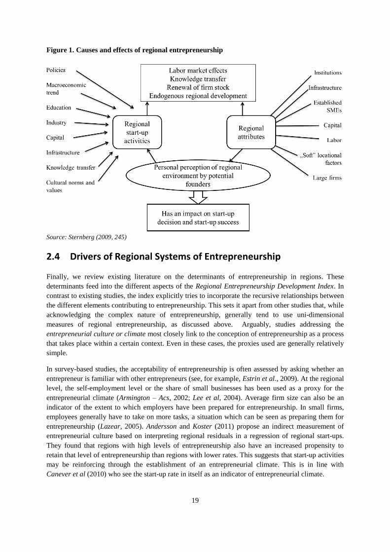
Figure 1. Causes and effects of regional entrepreneurship
Source: Sternberg (2009, 245)
2.4 Drivers of Regional Systems of Entrepreneurship
Finally, we review existing literature on the determinants of entrepreneurship in regions. These
determinants feed into the different aspects of the Regional Entrepreneurship Development Index. In
contrast to existing studies, the index explicitly tries to incorporate the recursive relationships between
the different elements contributing to entrepreneurship. This sets it apart from other studies that, while
acknowledging the complex nature of entrepreneurship, generally tend to use uni-dimensional
measures of regional entrepreneurship, as discussed above. Arguably, studies addressing the
entrepreneurial culture or climate most closely link to the conception of entrepreneurship as a process
that takes place within a certain context. Even in these cases, the proxies used are generally relatively
simple.
In survey-based studies, the acceptability of entrepreneurship is often assessed by asking whether an
entrepreneur is familiar with other entrepreneurs (see, for example, Estrin et al., 2009). At the regional
level, the self-employment level or the share of small businesses has been used as a proxy for the
entrepreneurial climate (Armington – Acs, 2002; Lee et al, 2004). Average firm size can also be an
indicator of the extent to which employers have been prepared for entrepreneurship. In small firms,
employees generally have to take on more tasks, a situation which can be seen as preparing them for
entrepreneurship (Lazear, 2005). Andersson and Koster (2011) propose an indirect measurement of
entrepreneurial culture based on interpreting regional residuals in a regression of regional start-ups.
They found that regions with high levels of entrepreneurship also have an increased propensity to
retain that level of entrepreneurship than regions with lower rates. This suggests that start-up activities
may be reinforcing through the establishment of an entrepreneurial climate. This is in line with
Canever et al (2010) who see the start-up rate in itself as an indicator of entrepreneurial climate.

20
Existing studies, such as these, help to inform the construction of the index as they pinpoint different
relevant elements that explain regional entrepreneurial activity, as well as its outcomes. Given the goal
of the index to also address the quality aspect of entrepreneurship, and with it development issues, we
specifically include determinants of high-quality entrepreneurship. We here review the existing
literature in five broad interrelated categories that describe pertinent elements in the entrepreneurship
process: 1) Spatial externalities, 2) Clustering, networking, social capital, 3) Education, human capital
and creativity, 4) Knowledge spillovers, universities and innovation 5) The state.
2.4.1 Spatial externalities
A. Agglomeration economies
Several pieces of work have found that urban areas host more entrepreneurship activities than non-
urban regions in the same country (see Sternberg, 2004; Acs et al., 2008). Two important aspects of
urban areas relate to this category of environmental resource; the demand for and supply of
entrepreneurship (Keeble – Walker, 1994, Reynolds 1994, Verheul et al., 2002).
The literature on economic development suggests that a dense, urbanized context reflects the
advantages of agglomeration, presumably including the benefits of access to customers and resources
(Delmar – Davidsson, 2000). Spatial proximity of knowledge owners and potential users therefore
appears to be critical for the transmission of tacit knowledge (Polanyi, 1966). Urban areas attract
younger, better educated adults, thereby increasing the pool of potential entrepreneurs. People living in
urban areas are more likely to be aspiring entrepreneurs, nascent entrepreneurs and business founders
compared to individuals living in rural areas (Rotefoss – Kolvereid, 2005; Bosma et al., 2008). In the
case of Finnish regions, Kangasharju (2000) found that the presence of small firms and economic
specialization, as well as urbanization and agglomeration have a consistent positive effect on firm
formation.
Most of the theoretical arguments in favor of agglomeration (in an economic sense) also hold true for
economic growth in many regional types (see McCann – van Oort, 2009; or argument in favor of
connectivity see McCann – Acs, 2011; Rodríguez-Pose, 2012).
B. Population growth, size of the region and market potential
The regional demand for entrepreneurship is often linked to population growth and population density
(Bartik 1989; Audretsch – Fritsch, 1994; Keeble – Walker, 1994; Reynolds 1994; Reynolds et al.,
1994, 1999; Delmar – Davidsson, 2000). As Keeble and Walker (1994) and Reynolds (1994) point out,
population growth and high population density undoubtedly affect the number of entrepreneurs. The
literature has also shown that SMEs favor countries within a low geographical distance with a large
market potential (Ojala – Tyrväinen, 2007). Large markets allow firms to develop and benefit from
economies of scale and could give incentives to entrepreneurship and innovation (Yasuhiro et al.,
2012; European Commission, 2010).
The literature on economic growth and regional development has also shown that both entrepreneurial
activity and agglomeration have a positive and statistically significant effect on technological change,
having indirectly an effect on regional development. In addition, the spillover impact in knowledge
production is positively related to the size and density of the region due to the richer network linkages
and the wider selection of producer services in larger areas (Varga, 2000; Acs – Varga, 2005).

21
All this results in more entrepreneurship activities (also in relative terms), the larger is the population
of the urban area. The very recent “knowledge spillover theory of entrepreneurship” (Acs et al., 2009,
Audretsch et al., 2006, Audretsch – Keilbach, 2007) builds on these findings. A high level of regional
research and development (R&D) activity increases regional opportunities to start new knowledge-
based businesses, and such a high level of R&D intensity is supposed to increase the creation of new
technological knowledge and, through localized knowledge spillovers, the level of opportunities for
start-ups in knowledge-based industries. Consequently, ideas and knowledge flow faster while the
provision of ancillary services and inputs is also greater in large cities.
Entrepreneurial activity, as a result, has been found to be greater in densely populated regions
(Sternberg, 2004). For Germany, Wagner and Sternberg (2004) found that the propensity to become
self-employed is higher for persons who live in more densely populated and faster growing regions
with higher rates of new firm formation. The authors also found that in densely populated regions
higher prices of land and risk aversion can have a negative effect on new firm formation.
C. Industrial specialization
One aspect of industry specialization that is important for regional economic growth is the type of
entrepreneurial activity. While there are many different type of start-up firm one type of specialization
is especially important. That is while many firms are similar a subset of these is about scale and wealth
creation. This subset of high impact firms is responsible for most of the job creation, innovation and
growth.
Other types of agglomeration patterns are also associated with entrepreneurship. In the case of Finnish
regions, economic specialization was shown to have a positive effect on regional firm formation
(Kangasharju – Pekkala, 2004). The degree of industrial specialization provides the opportunity for
industries to explore localization economies also in the case of Greek regions (Fotopoulos – Spence,
1999). In the case of Italian regions, the production structure and mainly local productive
specialization appear to be one of the most important determinants for explaining firm formation and
regional differentiation. The high specialization of the industrial environment, associated with an over-
representation of small businesses, is positively associated with high new firm formation rates
(Garofoli, 1994).
Although specialization in specific industries may positively impact on firm formation, the findings
contrast with the more general ideas from agglomeration theory as discussed in the above, and the
spill-over theory of entrepreneurship. Both advocate that a diverse set of actors will stimulate the
discovery and development of new entrepreneurial opportunities. Audretsch and Keilbach (2008)
confirm this empirically for Germany.
2.4.2 Clustering, networking, social capital
A. Clustering
The literature has also explored the positive impact of other types of industrial concentration, for
example, the effect of clusters, defined as geographically proximate groups of interconnected firms
and associated institutions in related industries, on new firm formation (for the case of German regions
see Rocha – Sternberg, 2005). Industrial clusters can enhance new firm births as well as the
productivity of existing firms. Linkages among firms and related institutions, which are the key
22
characteristics of the cluster phenomenon, can serve as an important determinant of new firm
formation.
The network aspect of clusters helps nascent entrepreneurs to find resources and information easier
and faster than in an isolated environment (Koo – Cho, 2011). Sternberg and Litzenberger (2004) also
found that the existence of one or several industrial cluster(s) has a positive impact on the number of
start-ups and attitudes. For the US, Koo and Cho (2011) found that clusters based on knowledge
sharing (i.e., knowledge-labor cluster) significantly affect new firm formation, whereas clusters based
on market transactions (i.e., value-chain cluster) do not seem to play a role. Delgado et al. 2010, also
for the US, found that after controlling for convergence in start-up activity at the region-industry level,
industries located in regions with strong clusters (i.e. a large presence of other related industries)
experience higher growth in new business formation and start-up employment. Strong clusters are
associated with the formation of new establishments of existing firms, thus influencing the location
decision of multi-establishment firms and contributed greatly to start-up firm survival.
B. Networking (role models)
Entrepreneurs may become role models and encourage other individuals to consider business
ownership. Evidence suggests that areas with a high proportion of small firms may provide role
models for potential entrepreneurs (Fritsch, 1992; Reynold, 1994, Garofoli, 1994; Hart – Gudgin,
1994; Love, 1995; Malecki, 1997; Spilling, 1996). Davidsson et al. (1994) claim that the availability of
role models and people with relevant work experience is the single most important determinant of
regional variation in new formation rates. Their study, conducted in Sweden, reveals that regions with
a high proportion of small firms have significantly higher new firm formation rates. Apart from SME
presence, networks in general influence the decision to become an entrepreneur as networks and peer
groups may provide role models. Therefore, a region with high levels of entrepreneurship may further
encourage new entrepreneurial initiatives because it is easier to access information or resources from
other entrepreneurs (Bosma et al., 2012). The self-reinforcing effect of role models may also go some
way in explaining the persistence in the regional distribution of start-up rates (Andersson – Koster,
2011; Fritsch – Mueller, 2007; Fritsch –Wyrwich, 2012).
C. Social capital
There are different conceptions of social capital, which each relate to entrepreneurship (Westlund –
Bolton, 2003). First, social capital can be seen as the network through which valuable resources for the
start-up of a new firm can be attained. This view is in line with Bordieu’s conception of social capital
(Bourdieu – Waquant, 1992). Secondly, value can be derived from the social network itself through
the shared values, information in the social group. This mimics a conception of social capital that puts
more emphasis on the social network itself – rather than the resources for production derived from it -
as the defining element (see, for example, Coleman 1990). Without going into a detailed discussion on
definitions and conceptions of social capital, this simple dichotomy helps structure the empirical
examples that allude to social capital.
We have already mentioned a number of studies that stress how important resources for firm
formation are derived from the social network. This includes access to finance (Kerr –Nanda, 2009),
access to ideas and the recognition of opportunities (Shane – Venkataraman, 2000) and access to labor
in the form of friends and family helping out in the business (Dahl and Sorenson, 2009). In this view,

23
the benefits from social capital may in principle be available to all members of the social network, but
once allocated they are rival goods and only accrue to the entrepreneur (or firm) accessing them.
This is in contrast with the other type of social capital in which values, ideas and acceptance vis-a-vis
entrepreneurship are shared in the social group. The effects are embedded in the group and become a
public good for the members of the group. Schutjens – Völker (2010) stress this type of social capital
as they see it as a culture of interaction among people. Social capital promotes regional learning both
within a region and beyond, as it reinforces the openness to the ideas of others. The literature on role
models can also be reframed in this conception of social capital. The role models, if relevant in a
social group, can have an effect on the whole social network. Likewise, the occupational structure of
regions may indicate the human capital endowments of the people and as a result their propensity of
starting a firm. It can also be seen as a crude measure of the existence of shared values and beliefs that
may or may not stimulate entrepreneurship (see, for example, Hart – Gudgin, 1994).
From the results reviewed here, it is apparent that social capital is seen as an important part of the
entrepreneurial decision that also explains an important part of the idea why entrepreneurship is an
inherent local phenomenon (Fornahl, 2003). Still, it is seems difficult to empirically pinpoint the
effect of social capital. If it seen as a means of accessing resources, the availability of the resources
can just as well be seen as the explanatory factor; if it seen as a value-laden network affecting
entrepreneurship, it is difficult to measure directly.
2.4.3 Education, human capital and creativity
A. Education and vocations
Education has been related in the literature to knowledge, skills, problem-solving ability, discipline,
motivation and self-confidence (Cooper et al., 1994). There seems to be agreement that attaining a
high level of education positively influences the probability of becoming involved in business start-up
processes (Cooper et al., 1994; Bates, 1995; Delmar and Davidsson, 2000). In addition, schooling has
an important impact on successful entrepreneurship. Van der Sluis et al. (2008) review over 100
studies on the issue and they find a marginal return of 6.1% to an additional year of schooling. For
wage income, they find an even larger marginal effect, suggesting that other factors are relatively
important in explaining income from self-employment. Iversen et al. (2010) reinforce this observation
in their study of returns to self-employment in the Danish labor market. They find a similar overall
marginal effect of 6,5%, but also show that the effect is highly influenced by those that have enjoyed
very long episodes of schooling. The marginal effect only increases significantly for those with at least
17 years of schooling. The level of education, however, is not the only determinant of self-
employment (success). Also the type of study influences the incidence of self-employment (see, for
example, Falk – Leoni, 2009). This may have to do with the content of the study and to what extent
the content prepares the graduate for self-employment, but it is also importantly influenced by the
labor market arrangements that are common in the industries the graduates are likely to be active in. In
the Netherlands, for example, General Practitioners are generally organized in a specific legal
arrangement that involves self-employment.
Similarly, Glaeser and Kerr (2009) find that abundant workers in relevant occupations strongly predict
regional entry. For the case of Greek regions, the supply of skilled manufacturing labor was found to
attract moving firms and stimulate new firm formation (Fotopoulos – Spence, 1999). Human resources
in science and technology have a strong impact on the number of new start-ups and new jobs. They are

24
typically the workers who come up with new ideas and put them into practice, which leads to more
new and more innovative and productive firms and higher creation of jobs (Kern – Runge, 2009).
Entrepreneurs with high level of education are more likely to have a role model, and the likelihood
that these entrepreneurs view their role models as crucially important is significantly higher (Bosma et
al., 2012).
Universities can be an important anchor tenants for regional clusters (Hausman, 2012; Chatterji et al,
2013). Certain studies have shown that long-run employment and wages increased quickly in
industries more closely related to local universities’ pre-existing strengths in innovation. This effect
was realized through the entrance of new firms and, especially, the expansion of multi-unit firms into
the area. The power of local universities to engender economic growth is also studied by Moretti
(2004) and Glaeser and Saiz (2003).
B. Creative class, talent
According to the “economic geography of talent” hypothesis put forward by Florida (2002a, b) highly
qualified people tend to live in close spatial concentration. Such regions are characterized by low
barriers to entry for well-educated, young workers who are attracted in particular by cultural diversity
and openness toward the new and the “different”. Up until then a small number of empirical studies on
the spatial mobility and entrepreneurial activities of the member of Florida’s “creative class” (Florida
2002b, Boschma – Fritsch, 2009) show that they are highly mobile in a spatial sense, very
discriminating when choosing locations and that they represent a high level of entrepreneurial
potential. Given the fact that creative people are more inclined to economic independence, it seems
plausible that they have a higher propensity to start a business comparing to non-creative people.
Consequently, regions with a higher proportion of creative people (that is, mainly, urban areas) should
also be characterized by higher start-up rates than rural areas (Sternberg, 2012). For the case of Italian
regions, Piergiovanni et al. (2009) observed that the regional employment growth is influenced by the
prevailing patterns of sectoral specialization and by the rate of growth of the share of firms in creative
industries (artists’ and writers’ creation, fashion design, advertising, architectural and engineering
activities and industrial design, software, etc.). Given the preference for attractive urban regions, the
positive effect of agglomeration may therefore partially be a sorting effect of entrepreneurial talent
congregating in certain areas.
2.4.4 Knowledge Spillovers, Universities and Innovation
A. Knowledge Spillovers
As long as the knowledge necessary for technological change is codified (i.e., it can be studied in
written forms either in professional journals and books or in patent documentations), access to it is not
essentially constrained by spatial distance; among other means, libraries or the Internet can facilitate
the flow of that knowledge to the interested user, no matter where the user is located. However, where
knowledge is not codified, because it is private, or not yet completely developed, or is so practical that
it can only be transmitted while being applied, the flow of it can only be facilitated by personal
interactions. Thus, for the transmission of such tacit knowledge spatial proximity of knowledge
owners and entrepreneurs appears to be critical (Polanyi, 1967).
Adam Jaffe (1989) was the first to identify the extent to which university research spills over into the
generation of commercial activity. His statistical results provided evidence that corporate patent
25
activity responds positively to commercial spillovers firm university research. Building on Jaffe’s
work, Feldman (1994) expanded the knowledge production function to innovative activity and
incorporated aspects of the regional knowledge infrastructure. She found that innovative activity is
conditioned by the knowledge infrastructure and responds favorably to spillovers from university
research at the state level, strengthening Jaffe’s findings.
Varga (1998) built further on this solid foundation. His main concern was whether university-
generated economic growth observed in certain regions and from selected industries can be achieved
by other regions. He extends the Jaffe-Feldman approach by focusing on a more precise measure of
local geographic spillovers. Varga approaches the issue of knowledge spillovers from an explicit
spatial econometric perspective and for the first time implements the classic knowledge production
function for 125 Metropolitan Statistical Areas, yielding more precise insights into the range of spatial
externalities between innovation and research and development.
The Jaffe – Feldman – Varga research into R&D spillovers takes us a long way towards understanding
the role of R&D spillovers in knowledge-based economic development. A host of recent empirical
studies have confirmed that knowledge spillovers are geographically bounded (Acs et al., 1992, 1994;
Jaffe et al., 1993; Audretsch – Feldman, 1996; Anselin et al, 1997; Keller 2002).
B. Innovation
The literature of innovation systems, even if highly influenced by the work by Schumpeter seems not
to have a clearly defined role for entrepreneurship. Radosevic (2007) ascribed this absence to the
predominantly institutional emphasis of the innovation system literature, which has made it difficult to
accommodate the individual-centric perspective of the entrepreneurship literature (Shane, 2003). For
instance, in the institutional tradition of the National Systems of Innovation literature, institutions
engender, homogenize, and reinforce individual action: it is a country’s institutions that create and
disseminate new knowledge and channel it to efficient uses. In this perspective, individual action is
either not considered or is supposed to happen automatically, subject to the homogenizing influences
of the institutions. This routine-reinforcing perspective of the systems of innovation literature has
proven difficult to reconcile with the individual-centric, routines-breaking emphasis of the
entrepreneurship literature (Radosevic, 2007; Schmid, 2004).
The literature highlights three main problems typical of regional innovations systems that need to be
addressed: (1) fragmentation, (2) absence of key resources, and (3) negative lock-in (Tödtling –Trippl,
2005).
Fragmentation can be a problem in regions where all the necessary components of a successful
innovation system already exist. This means that strong actors are present in all three subsystems and
that there is an institutional framework well suited to these actors. The problem of fragmentation
occurs when the authors are not aware of each other and/or when they do not act in harmony with each
other. One reason may be that there is an institutional and/or functional mismatch. An example of
institutional mismatch can be the absence of an overall collective action. Functional mismatch, where
the functions that the innovation system supports do not result in mutually reinforcing synergies, is
experienced in the case of a lack of coordination.
The absence of key resources that are necessary for a proper functioning of an innovation system, such
as the regional presence of human capital, represents a grand challenge in many regions. In this
situation the region faces the challenge of attracting key resources either by influencing the regional
26
supply or by stimulating the regional actors to meet the resource needs through contracts with actors
outside the region. This may also be the case for entrepreneurship.
Finally, negative lock-in represents the most difficult problem for regions today. Negative lock-in may
occur when regional specialization has emerged in a sector that in the medium or long term does not
have good growth potential, but which may still be an important part of the region’s industrial identity.
In this context, it is not necessarily just lock-in in obsolete technology that is in question, but also
lock-in in skills and market terms. The main challenges for the development initiative in such a
situation is to influence those actors who represent or support the specialization that is risky or
problematic in the long term to be open to new inspiration or to change direction. The prerequisites for
avoiding this kind of negative lock-in are probably better in regions with a diversified economy within
related industries, as this provides opportunities for new combinations of existing knowledge and thus
renewal in terms both of technology and of market orientation.
Additionally, Henning et al (2010) describe a final issue that is complementary to all the previous ones
(4) inconsistencies between the regional economic structure and the priorities of the regional policy.
A lack of correspondence between the policy measures implemented by the actors in the innovation
system’s support structure and, on the other hand, the regional economic structure, can result in an
inefficient support structure and an unexploited regional innovation capacity.
C. Protection of property rights
Based on broad historical studies such as North (1981) and Rosenberg and Birdzell (1986) or Rodrik et
al. (2004) and Acemoglu and Johnson (2005), it is now widely recognized that protection of property
rights is of fundamental importance for economic growth. Aidis et al. (2010) find the property right
system to play a pivotal role in determining entrepreneurial entry, in particular in low and middle
income countries while Johnson et al. (2002) also provide evidence that weak property rights
discourage entrepreneurs from reinvesting profits. Depending on the level of protection of property
rights different types of entrepreneurship will be favored. For example, strong private property rights
will help productive entrepreneurship to thrive as the entrepreneurial rents are expected to be retained.
In contrast weaker property rights will favor the establishment of unproductive entrepreneurial
activities or other productive activities such as private security services, created to solve the lack of
security in the environment. Henrekson (2007) also points that in recent years the excessive protection
of property rights is likely to impede productive entrepreneurship.
D. Finance
Small and newly established firms are more dependent on equity financing than large, well-established
firms. Individual wealth positions have been considered as an important determinant in explaining the
propensity of individuals to become entrepreneurs and to innovate in the case of SMEs (Parker, 2004).
However, in the case of pure traditional measures of entrepreneurship, the literature seems not to be
conclusive in determining the effect of saving rates on entrepreneurship. Young (1992) compares the
cases of Singapore and Hong Kong and concludes that having GDP rates very similar but double the
saving rates in Singapore, the Hong Kong economy appears to be more entrepreneurial. In the case of
the mature welfare states in Northern Europe the entrepreneurial activity as conventionally measured
seems to be low. Welfare state provisions such as unemployment or sick-leave benefits, income-
dependent pensions and subsidizing health and care services remove a number of savings motives for
27
the individual and this could be the reason why entrepreneurs do not have at their disposal the required
savings to start a business.
Henrekson (2007) also points that the composition, and not just the volume, of saving is of importance
for entrepreneurship. For this reason, any social arrangement that channels savings and asset control to
large institutional investors is likely to limit the supply of financial capital to potential entrepreneurs.
These issues also point to the question of taxation. The literature argues that taxation is another
institutional barrier that affects entrepreneurial activities. However, the analysis of how taxation may
affect entrepreneurship in the aggregate data analysis is complex and sometimes cannot be explicitly
captured.
While it is hard to deny the importance of banks in the provision of traditional type of debt especially
in the European Union, over the last two decades some alternative forms of mainly equity financing
has been emerging. Entrepreneurial finance refers to the alternative sources of capital (Denis, 2004;
Winton – Yerramilli, 2008). For startups and entrepreneurial firms venture capital is particularly
important (Berger – Udell, 1998; Gompers et al., 2005; Kanniainen – Keuschnigg, 2004). Beside
money, venture capitalist and business angels provide various assistance and help to the generally
inexperienced young business owners (Gompers, 1995, Helman – Puri, 2002). Most start-ups have no
other choice but to approach their relatives, friends or other acquaintances if the founders own savings
are not enough for launching the business (Mason, 2007). GEM data based analyses highlight that the
amount of informal investment exceeds that of the formal venture capital by 8-20 times. At the same
time the average amount invested in one business by venture capitalists can be hundreds times higher
than that of the informal venture source of family members, friends and alike (Bygrave – Hunt, 2004;
Bygrave – Quill, 2007). Overall, the adequate supply of both formal and informal venture capital is
vital for providing the necessary fuel for high growth potential businesses in their critical phases of the
life cycle.
Both formal and informal investment, in particular angel finance, tends to concentrate to more
prosperous agglomerated areas (Florida – Smith, 1993; Jones-Evans – Thompson, 2009; Martin et al.
2002, Mason – Harrison, 2003). Spatial proximity is particularly important in certain high tech,
biotechnology or internet based sectors and clusters (Powell et al., 2002; Zook, 2008).
2.4.5 The Role of the State
A. Size of government
A large state sector is usually synonymous with generous levels of welfare provision, for example
unemployment benefits, pensions and child welfare for women in work. These benefits must be paid
for, and this is usually done by high levels of personal taxation, often within a progressive tax regime
in which high earners, such as successful entrepreneurs, pay higher marginal rates. This will reduce
the expected returns to entrepreneurial activity. Moreover, when the welfare system for those in
employment is generous, the opportunity cost of entrepreneurship is against other forms of
employment or non-participation in the labor force is raised. Taken together, these factors would
suggest that a larger state sector will reduce entrepreneurial activity (Aidis et al., 2010). Henrekson
(2005) found that a strong welfare state dampens entrepreneurial activity by taking away incentives for
starting a firm. The range of rules and regulations in place sometimes give opposing incentives for
firms and the effect of the institutional framework on firm dynamics is therefore essentially a net
effect for which a limited number of variables form a poor proxy (Henrekson – Johansson, 2011).
28
B. Regulations
The regulative institutions are those controlling systems that are legally sanctioned, such as laws and
regulations. Normative institutions, however, are not necessarily linked to any direct sanction system,
but are maintained by (often unconscious) moral considerations and are thus indirect sanction systems
(anyone who does not adhere to normative institutions loses his legitimacy and is marginalized in the
long run). Examples of normative institutions are perceptions of what is accepted as good business
practice in different contexts. Views on this may differ between industries, nations or regions. The
cognitive institutions are shaped by culture and daily routines/practices and are thus more or less taken
for granted by individuals. They are adhered to, therefore, without further reflection (Moodysson,
2007).
One example of this is the way in which problem-solving is conducted. In somewhat simplified terms,
one can say that regulative institutions are largely but not entirely formal (particularly with regard to
laws and regulations), while normative and cognitive institutions are to a significantly greater extent
informal (norms and values). The above classifications do, however, overlap to a certain extent. As
such, the three institutional types should not be regarded as distinctly separate categories, but rather as
interdependent, inseparable dimensions that together form the institutional framework that affects the
harmony of the innovation system by governing actors’ behavior towards each other and the outside
world. (Henning et al., 2010)
The literature has shown that the effect on entrepreneurship activity on regional development is driven
by the institutional context in which entrepreneurial activity takes place. Since Baumol (1990, 1993), a
literature has emerged suggesting that disparities in entrepreneurial activity between countries (or
regions) can be explained by the quality of their supporting institutions. Institutional theory has argued
that company behavior, including entrepreneurial choices, will be context specific (Meyer – Peng,
2005), and a literature has emerged to show that entrepreneurial activity is sensitive to the quality of
institutions (Batjargal, 2003; Henrekson, 2007; Sobel, 2008) as well as to the level of economic and
social development.
The institutional context can be either conducive or detrimental to the entrepreneurship. It is
reasonable to think that higher levels of corruption or weaker intellectual property rights will have a
negative impact on entrepreneurship. A favorable business environment, where entrepreneurial
activities are supported by institutions and a trustable governance system, will infer a positive effect in
the creation and impact of entrepreneurship (North, 1990, 1994; Baumol, 1993; Davidsson –
Henrekson, 2002).3
The degree of regulation of labor markets and wage-setting can be expected to influence incentives for
entrepreneurship, since it restricts the freedom of contracting and therefore curtails the possible
combinations of factors of production. The literature has found important differences between
countries in terms of labor market regulation.
3 Although the impact of institutions on entrepreneurship can vary depending on the stage of entrepreneurship
and aspects such as the stage of economic development of the country or region, in this section these two aspects
will be omitted. We then are going to consider as a whole the institutions that have an influence in
entrepreneurship creation and their impact non discriminating the stages of entrepreneurship.

29
Henrekson (2007) states that there are reasons to believe that strict employment security provisions,
and other regulations that restrict contracting flexibility, are more harmful for smaller and more
entrepreneurial employers. Another labor market arrangement that may impact on the incentives for
entrepreneurship is wage-setting institutions. Institutional pressures for wage compression are likely to
disadvantage smaller and more entrepreneurial businesses.
The cross-country comparative studies on the effect of labor market regulations on job counts can help
to understand some entrepreneurship and firm evolutionary patterns. Birch and Medoff (1994)
hypothesize that in the US the really good entrepreneurial firms become fast-growing gazelles and the
self-employment is fairly low in US. Oppositely, in Italy, the high regulatory environment with high
labor taxes make difficult and risky to grow businesses, such that they prefer to remain smaller
(Lazerson – Lorenzoni, 1999).
C. Corruption
Corruption has been seen as being negative for firm entry by raising the costs and therefore reducing
the returns to entrepreneurial activity (Anokhin – Schulze, 2009). Desai and Acs (2007) argue that a
corrupt environment may have negative supply side effects on entrepreneurs, and especially on those
with higher aspirations, leading them to satisfy their ambitions through rent seeking rather than the
formation of new firms. The effects of a corrupt institutional environment seem to have higher
negative effect on higher growth aspiration entrepreneurship. Its negative effect impact more highly on
potential new firms than incumbents, because incumbents have developed a higher resilience in
operating longer in corrupt environment which is highly uncertain (Aidis et al., 2008, 2010). Estrin et
al. (2012) find that the coefficient on freedom from corruption appears to be highly significant in
explaining employment aspirations by entrepreneurs.

30
3 DATA AND METHODOLOGY
3.1 Introduction
This section devotes its attention to the data description and to methodological issues of the Regional
Entrepreneurship and Development Index REDI. Index-building is a complex task that faces several
potential pitfalls, starting with the vague and various definitions of a concept like entrepreneurship.
Following Acs et al (2013a) we favor a complex perception of entrepreneurship and believe that this
complexity requires a composite index, as opposed to the single measures often used. The Systems of
Entrepreneurship (SE) theory is based on the following core assumptions:
1. Economic growth is ultimately driven by a trial-and-error resource allocation process, under
which entrepreneurs allocate resources towards productive uses;
2. This process is driven by individual-level decisions, but those decisions are conditioned by
contextual factors;
3. Similarly, the outcomes of individual-level entrepreneurial decisions are conditioned by
contextual factors;
4. Because of the multitude of interactions, country-level entrepreneurship is best thought of as a
system, the components of which co-produce system performance
While in the previous chapter we have provided an exact description of entrepreneurship, in practical
terms it is closer to a permeable frame than a closed box. Our approach to entrepreneurship measure
involves five important aspects.
1. First, we view entrepreneurship as a concept of quality rather than quantity.
2. Second, we consider both institutional and individual factors vital in measuring
entrepreneurship.
3. Third, measuring the pillars of entrepreneurship is based on a benchmark of the best five
percent existing achievement for each particular pillar.
4. Fourth, the averages of each 14 pillar values are equated to provide the same marginal effect.
This point is particularly important from the entrepreneurship policy point of view.
5. And fifth, we view the building blocks of entrepreneurship, the 14 pillars, not as independent
but as integrated elements of a system. We believe that the performance of the overall system
depends on the weakest pillar, and that a good performance in one pillar can substitute only
partially for a badly performing element of the system. A practical application of this theory is
the penalty for bottlenecks (PFB) methodology.
After this short introduction, we present the description of the applied data. The REDI has a six-layer
structure from sub-indicators, indicators, variables, pillars, sub-indexes. Here, we focus on the
individual and the institutional indicators and variables. Individual-level variables are based on
indicators from the GEM Adult Population Survey dataset except two innovation indicators that are
from the European Union data collection. For this report we used the 2007-2011 pooled GEM data.

31
There are two types of institutional variables, country level and regional ones. Our original idea was to
construct the institutional variables from fourteen country wide and fourteen regional indicators. The
later would have reflected to spillovers effective mainly in smaller than county level geographic areas.
However, in many cases we faced the lack of available data. Finally we ended up having eight
country-wide and thirteen regional indicators. Institutional variables are more complex, some of them
contain many sub-indicators. The sub-indicators are the basic building units of the institutional
indicators and variables. The sub-chapter provides a detailed description of the 76 sub-indicators, and
of the 40 variables we used to calculate the REDI scores for the mix of 125 NUTS1 and NUTS2
regions of 24 European Union countries.
In the following, we define and describe the structure of the Regional Entrepreneurship and
Development Index (REDI). We propose six level index-building: (1) sub-indicators (2) indicators (3)
variables, (4) pillars, (5) sub-indices, and, finally, (6) the super-index. The three sub-indices of
attitudes, abilities, and aspiration constitute the entrepreneurship super-index, which we call REDI. All
three sub-indices contain four or five pillars, which can be interpreted as quasi-independent building
blocks of this entrepreneurship index. Each of our 14 pillars is the result of the multiplication of an
individual variable and an associated institutional variable. In this case, institutional variables can be
viewed as particular (regional-level) weights of the individual variables.
The fourth part of this chapter summarizes the most important steps of our index creation. An
important novelty of our index-building is the way the pillars are combined (aggregated) into sub-
indices. Most indices simply use the (weighted) average of the pillars; others apply a dimension-
reduction methodology, such as factor analysis. We provide a different approach that takes into
account the fact that the pillars are only partially substitutable for each other. Relying on the Theory of
the Weakest Link (TWL) and the Theory of Constraints (TOC), we developed this new methodology,
which we call the Penalty for Bottlenecks (PFB). We believe that the basic claim of these theories—
that the performance of the system is determined by its weakest performing part and the pillars can
only be partially substitutable with one another—are true in the case of entrepreneurship. The PFB
relates the pillar values to the lowest pillar value. The penalty depends on the magnitude of the
differences; for greater deviation, the penalty is greater. We applied an exponential penalty function.
The PFB provides valuable policy suggestions for enhancing entrepreneurship by improving the
weakest pillar in the system.
In the last section we introduce a new indicator, the Average Bottleneck Efficiency (ABE) measure.
This efficiency indicator measures how much a country’s fourteen pillars are balanced.
3.2 Data description
As mentioned previously, our entrepreneurship index incorporates both individual-level and
institutional/environmental variables. Here we provide a full description of the data, the data collection
method and the calculation of the variables from the indicators and sub-indicators. All individual-level
variables except two are from the GEM survey. The institutional variables are obtained from various
sources. For the details, we refer to the Appendices.
3.2.1 REDI individual data description
In this part we review the individual data. The full list and description of the applied GEM individual
variables and indicators can be seen in Appendix A. For more information on the GEM methodology

32
we refer to Reynolds et al (2005). Bosma (2013) provides an update on the methodology and lists and
discusses the academic articles that are (partly) based on GEM data.
As previously mentioned, individual-level variables are based on the GEM Adult Population Survey
dataset. For this report we used the 2007-2011 pooled GEM data. For Estonia, 2012 was used since
this country only joined the GEM project in 2012. For 24 countries in the European Union, including
Croatia, it was possible to create the regional representation of the GEM dataset except Bulgaria,
Cyprus, Luxembourg, and Malta. In the case of 10 countries, GEM data were regionalized at NUTS1
level (Austria, Belgium, Greece, France, Germany, Italy, Netherlands, Poland, Romania, and United
Kingdom). For four additional countries the country level classification was equal to the NUTS1 level
classification. These are the Czech Republic, Latvia, Lithuania and Estonia. For the remaining 10
countries, GEM data were calculated at NUTS-2 level (Croatia, Denmark, Finland, Hungary, Ireland,
Portugal, Spain, Slovenia, Slovakia, and Sweden). In the case of Portugal, only those five NUTS-2
level data were available which belong to the Continente NUTS1 region. For Spain, the two small
African continent NUTS1 regions, Ceuta and Melilla were also excluded. Thus, we have calculated the
REDI for 24 countries which altogether contain a mix of 125 NUTS1 and NUTS2 regions.
It should be noted that some countries participated in GEM all years between 2007-2011, while others
participated just a few years (or even just one in the case of the Czech Republic). In order to achieve
satisfactory sample sizes for some of the regions in the classification listed above, we have included
2012 data for Austria, Estonia, Poland, the Slovak Republic and Sweden (see Table 1 for an
overview). For most of the regions, a satisfactory sample size was achieved. For 97 out of the 125
regions, the sample size exceeded 1,000 individuals. For four regions the GEM variables are based on
sample sizes lower than 300 cases and should therefore be taken with care. These include Bremen
(Germany), Algarve (Portugal), Saarland (Germany) and Alentejo (Portugal). Other regions with
relatively limited coverage include Poludniowo-Zachodni (Poland), Mecklenburg-Vorpommern
(Germany), Thüringen (Germany) and Bratislavsky Kraj (Slovakian Republic), all with sample sizes
between 400-500.
In this respect it should also be noted that NUTS classifications are not always equally comparable in
terms of region/population sizes; in fact for some countries a mix between NUTS1/NUTS2 or
NUTS2/NUTS3 may be beneficial, dependent on the purpose of the analysis. For instance, the NUTS1
region of Bremen is limited to the core urban area and is much smaller in scope than for example the
large NUTS1 region of Bavaria, which includes Munich. For the REDI indicators the abovementioned
classification was adopted consistently.
In order to retrieve regional indicators from the individual level data, individual cases have been
aggregated bearing in mind discrepancies in regional age & gender patterns between the GEM Adult
Population Survey samples and those emerging from official national statistics and published by
Eurostat. Hence, an individual weighting variable corrects for the under- or overrepresentation of a
particular age/gender group in each of the 125 regions. The age groups considered are 18-24 years, 25-
34 years, 35-44 years, 45-54 years and 55-64 years.

33
Table 1. GEM Adult Population Survey Details by Country
Country Sample size 18-64 years Basic Class. Years included Nr. of regions
Austria 6,544 Nuts1 2007 & 2012 3
Belgium 11,431 Nuts1 2007-2011 3
Croatia 8.516 Nuts2 2007-2011 3
Czech Republic 2,005 Nuts1 2011 1
Denmark 9,975 Nuts2 2007-2011 5
Estonia 1,721 Nuts2 2012 1
Finland 10,034 Nuts2 2007-2011 5
France 7,994 Nuts1 2007-2011 8
Germany 20,595 Nuts1 2008-2011 16
Greece 9,962 Nuts1 2007-2011 4
Hungary 9,417 Nuts2 2007-2011 7
Ireland 5,899 Nuts2 2007; 2010-2011 2
Italy 10,934 Nuts1 2007-2010 5
Latvia 10,015 Nuts2 2007-2011 1
Lithuania 2,003 Nuts2 2011 1
Netherlands 12.484 Nuts1 2007-2011 4
Poland 4,003 Nuts1 2011 & 2012 6
Portugal 6,036 Nuts2 2007; 2010-2011 3
Romania 8,453 Nuts1 2007-2011 4
Slovak Republic 2,000 Nuts2 2012 4
Slovenia 14,090 Nuts2 2007-2011 2
Spain 131,533 Nuts2 2007-2011 17
Sweden 7,862 Nuts2 2007; 2010-2012 8
United Kingdom 72,296 Nuts1 2007-2011 12
Total sample 387,802 125
In most cases - eleven out fourteen – the individual indicators were used directly as variables. In the
remaining three cases we multiplied two indicators to calculate the variables. The New Product and
the New Technology variables combine together a GEM based and another regional level innovation
variable derived from the Poli-KIT database (Capello – Lenzi, 2013). The Prod Innovation and the
Tech Innovation indicators serve to correct for the potential bias in the GEM’s self-assessed
questionnaire. The Informal investment variable is a result of the multiplication of the mean amount of
informal investment (Informal Investment Mean) and the prevalence of informal investment (Business
Angel), both of them are coming from the GEM survey. Therefore, Informal investment combines
together tow aspect of informal finance providing a more accurate measure about the availability of
startup capital of a region. For details, see Appendix A. The standard errors of the GEM Adult
Population Survey base individual variables for each 125 regions are in Appendix B.
3.2.2 REDI institutional data description
Since the GEM dataset lacks the necessary institutional/environmental variables, we complete it for
the index with other widely used relevant data derived from different sources. These are the
followings:
EUROSTAT Regional Database
United Nations, Department of Economic and Social Affairs, Population Division
EU Regional Competitiveness Index 2010
World Bank – World Development Index,

34
Legatum Prosperity Index,
World Economic Forum,
EU QoG Corruption Index,
Heritage Foundation database,
ESPON database,
Cluster Observatory database,
DGRegion Individual Datataset (not-published),
Groh et al (2012) Global Venture Capital and Private Equity Country Attractiveness Index,
OECD-PISA database.
A potential criticism of our method – as with any other index – might be the apparently arbitrary
selection of institutional variables and the neglect of other important factors. In all cases, we aimed to
collect and test alternative institutional factors before making our selection. Our choice was
constrained by the limited availability of data in many regions. The selection criteria for a particular
institutional/environmental variable were:
1. The potential to link logically to the particular entrepreneurship variable
2. The clear interpretation and explanatory power of the selected variable; for example, we have
had interpretation problems with the taxation variables4
3. Avoiding the appearance of the same factor more than once in the different institutional
variables5
4. The pillar created with the particular variable should positively correlate to the REDI.
To eliminate potential duplication, instead of using existing complex institutional variables offered by
different research agendas, we created our own complex indexes using relevant simple indicators or
sub-indicators.
Basically we apply a single indicator only in one case that is GERD (Gross Domestic
Expenditure in Research & Development as a percentage of GDP) used to measure
technological development.
In seven cases – Quality of Education, Social Capital, Open Society, Business Environment,
Absorption Capacity, Business Strategy, and Financial Institutions – the application of a
complex measure (using both country level and regional level indicators) proved to be more
useful than using one single indicator. Most of these indicators are complex creatures by
4 A former version of our index (Acs – Szerb, 2009) was criticized because we did not incorporate the taxation
effect (A European Paradise, p. 25). While it is true that high taxation can be harmful for entrepreneurship,
ceteris paribus, it should not be forgotten that high-taxation countries can provide better public services and an
environment favorable to business startups. While Scandinavian countries have high taxation, they also lead the
ranks in government effectiveness and regulatory quality, as reported by the World Bank Aggregate Governance
Indicator dataset (http://info.worldbank.org/governance/wgi/index.asp). 5 There is only one duplication in the data set we could not avoid: The corruption appears in the Corruption in
the Social capital institutional variable and also in the EU QoG INDEX.

35
themselves. For example the Business Environment variable consists of the Business Freedom
country level and the EU QoG INDEX regional level indicators. The Business Freedom is the
most composite indicator including ten sub-indicators. The EU QoG INDEX reflecting to the
quality of the government in the particular region contains four sub-indicators.
In five cases - Market Agglomeration, Higher Education & Training, Innovation sub-index,
Clusters and Accessibility – we use only regional level institutional indicators. In the case of
the Business disclosure we could find only a country level institutional indicator as a measure
of the overall risk in a particular country.
In three cases, instead of using whole existing complex index, we applied only sub-indices that
were more relevant to entrepreneurship: for example Business Freedom is a component of the
Index of Economic Freedom, Social Capital Sub-Index is a subset of the Legatum Prosperity
Index, and the Depth of capital market is a sub-index of the Venture Capital and Private
Equity Index.
In this version, we apply the most recent institutional variable indicators available on June 30. 2013.
The full description of the institutional variables, indicators and sub-indicators their sources, the year
of the survey, and the calculation method for each institutional variable can be found in Appendix C.
As a general rule of regional level institutional variable calculation, if data were not available at
NUTS1 level, we calculated the population weighted mean of the available NUTS2 regions. In cases,
when both NUTS1 and NUTS2 regions were not available, NUTS0 (country level) were used as
substitutes. NUTS0 data were used in Germany, France and Finland, because the lack of
Technological Absorption data at NUTS1/NUTS2. We also endeavored to substitute other missing
NUTS1 or NUTS2 level data (for detailed description see Appendix D).
For handling the extreme distribution of the institutional indicators we follow Annoni and Kozovska
(2010) method. They built on the Box-Cox transformation in the cases the absolute value of skewness
– a measure of the asymmetry of distribution – exceeds the absolute value 1. We apply this Box-Cox
transformation method to improve the distribution of those indicators that are out of the [-1,1] range
of skewness (Annioni – Kozovska, 2010, pp. 52-53)
The skewness, the degree of the asymmetry of distribution is calculated as the following:
(1)
is the skewness,
n is the number observed values for the indicator,
x is the arithmetic mean
s is the standard deviation.
The Box-Cox transformations are a set of power transformations for skewed data, and depend on
parameter λ.
(2)

36
Following Annioni and Kozovska (2010) we set
λ = 2 if κ ≤ -1 (left or negative skewness)
λ = -0.05 if κ ≥ +1 (right or positive skewness)
3.3 The structure of the Regional Entrepreneurship and
Development Index
Based on the definition of entrepreneurship we propose a six level index-building: (1) sub-indicator
(2) indicators (3) variables, (4) pillars, (5) sub-indices, and, finally, (6) the super-index. The three sub-
indexes of attitudes, abilities, and aspirations constitute the entrepreneurship super-index, which we
call the Regional Entrepreneurship and Development Index (REDI). The sub-indexes compose the
pillars. Pillars are the most important layers in the index structure because they provide the basis of the
Penalty for Bottleneck (PFB) analysis and entrepreneurship policy. Each of the fourteen pillars
consists of an institutional and an individual variable. The 40 indicators are the building blocks of the
variables. Some institutional indicators are complex creatures by themselves adding up to 76 sub-
indicators altogether. (For more details see Appendix E).
Figure 2 provides a more detailed picture of the sub-indexes, the pillars and its variables.
Figure 2. The structure of the Regional Entrepreneurship and Development Index
REGIONAL ENTREPRENEURSHIP AND DEVELOPMENT INDEX
Entrepreneurial Attitudes
Sub-Index
Entrepreneurial Abilities
Sub-Index
Entrepreneurial Aspirations
Sub-Index
Pillars
Op
po
rtun
ity P
erce
ptio
n
Sta
rt-up
Sk
ills
Risk
Acce
pta
nce
Netw
ork
ing
Cu
ltura
l Su
pp
ort
Op
po
rtun
ity S
tartu
p
Tec
hn
olo
gy
Ad
op
tion
Hu
ma
n C
ap
ital
Co
mp
etition
Pro
du
ct Inn
ov
atio
n
Pro
cess In
no
va
tion
Hig
h G
row
th
Glo
ba
lizatio
n
Fin
an
cing
Variables
Ma
rket
Ag
glo
mera
tion
Op
po
rtun
ity Rec
og
nitio
n
Qu
ality
of E
du
catio
n
Sk
ill Percep
tion
Bu
siness R
isk
Risk
Acc
epta
nce
So
cial C
ap
ital
Kn
ow
En
trepren
eurs
Op
en so
ciety
Ca
reer S
tatu
s
Bu
siness E
nv
iron
men
t
Op
po
rtun
ity Mo
tivatio
n
Ab
sorp
tion
Ca
pa
city
Tec
hn
olo
gy L
evel
Ed
uca
tion
an
d T
rain
ing
Ed
uca
tion
al L
evel
Bu
siness S
tra
tegy
Co
mp
etitors
Tec
hn
olo
gy
tran
sfer
New
Pro
du
ct
Tec
hn
olo
gy
Dev
elop
men
t
New
Tec
h
Clu
sterin
g
Ga
zelle
Co
nn
ectiv
ity
Ex
po
rt
Fin
an
cial In
stitutio
ns
Info
rma
l Inve
stmen
t

37
Note: The REDI is a super-index made up of three sub-indices, each of which is composed of several pillars.
Each pillar consists of an institutional variable (denoted in bold) and an individual variable (denoted in bold
italic).
While the abilities and aspiration sub-indices (outlined below) capture actual entrepreneurship abilities
and aspiration as they relate to nascent and startup business activities, the entrepreneurial attitude
(ATT) sub-index aims to identify the attitudes of a region’s population as they relate to
entrepreneurship. It consists of five pillars.
Opportunity Perception is essential to recognizing and exploring novel business opportunities.
It combines the individual variable of the opportunity recognition of the population with the
Market agglomeration institutional variable. Market agglomeration reflects to the size of the
market in a particular region including the growth of the population, the level of urbanization
and the accessibility of the region.
It is also critical to have proper startup skills to be able to exploit these opportunities. Startup
Skills depend on the populations’ self-esteem about its ability to start successfully a business
(individual variable) and on the quality of education institutional variable. The Quality of
education has two components. A country level indicator serves to measure the value of
secondary education by the PISA test results. It is combined with a variable reflecting to the
presence of the creative class in a region.
Fear of failure can have a negative effect to start even a high potential business. The
magnitude of risk acceptance of the population is the individual variable part of Risk
Perception. On the institutional side the business disclosure rate of the country is used as a
proxy of general business risk. Here we lack a proper regional variable.
Personal networks are also vital for successful startups. The individual variable, knowing an
entrepreneur personally (Know entrepreneur) is mixed together with the country level social
capital and a regional level technological readiness variable to get the Networking pillar.
While social capital proxies the human part of potential networking, the technological
readiness reflects to the availability of the internet in the regions.
Cultural Support, the acceptance, the encouragement and the support of successful
entrepreneurs are important ingredients of attitudes. The individual variable Carrier status
contains the view of the population about the carrier possibilities and the social status and
respect of entrepreneurs. Open society is the institutional variable of Cultural Support
containing a country level (Personal freedom) and a regional level indicator (Corruption).
Personal freedom measures countries’ performance in individual freedom and social tolerance.
The persistence of corruption could easily undermine believes that clear rules and individual
capabilities determine the reward structure of a region.
The entrepreneurial abilities (ABT) sub-index is principally concerned with measuring some important
characteristics of the entrepreneur and the startup with high growth potential.
An important aspect of high growth potential is the drive for startups. Opportunity Startup
mixes together the opportunity motivation of the population (individual variable) with the
favorability of the business environment (institutional variable). Business environment has a

38
country wide aspect as the freedom to start and operate business (Business freedom), and a
regional aspect, the quality of local government (EU QoG Index).
The sectorial composition of startups could also be a sign of potential high growth. The
Technology Adoption pillar highlights the role of technology and creative sectors. We use the
percentage of the young and nascent businesses that belong to a technology-intensive or
creativity sectors (Technology level) as individual variable. The institutional variable
(Absorption capacity) measures the technological readiness of the firms in a country and the
regional level of employment in knowledge intensive and high technology firms.
Most owners/managers of high growth potential businesses are educated persons. Moreover, it
is also important to find such employees who have received some training to have an updated
knowledge. The Human Capital pillar has two ingredients: the share of early phase
entrepreneurs who have over secondary level of education (Educational level) is merged
together with the involvement of the region’s population in training and life-long learning
(Education and training).
Those businesses that face a low level of competition could grow faster than businesses with
many competitors. The individual variable of Competition is the number of competitors,
benchmarking those ventures that have not too many competitors. The institutional variable is
Business strategy measuring the country’s nature of competitive advantage and the regional
level sophistication of the businesses. Unique products, processes and the number of
employees working in sophisticated sectors serve as benchmarks.
The entrepreneurial aspiration (ASP) sub-index refers to the distinctive, qualitative, strategy-related
nature of entrepreneurial activity. Entrepreneurial businesses are different from regularly managed
businesses, thus it is particularly important to be able to identify the most relevant institutional and
other quality-related interaction variables.
Product Innovation reflects not only to the newness of the product (individual component) but
also on the ability of the businesses in the region to create such products. Ultimately, the
regional level institutional variable (Technology transfer) reflects to the regions’ potential to
patent and to create scientific publications.
Technology Innovation has also two components. The individual variable (New technology)
measures the technology innovation potential of the businesses. The institutional variable
(Technology development) measures the financial aspect of innovation as the percentage of
Research and Development in the regional gross domestic product (GERD).
The High Growth pillar includes the percentage of gazelles as businesses with high growth
ambitions (Gazelle) and a clustering institutional variable. Clustering takes into account that
businesses are supported by other cluster members contributing to counterbalance missing
individual resources and to get further support for high growth.
A frequently noticed characteristic of high growth potential businesses is their capability to
internationalize. The Globalization pillar combines together the export potential, as measured
by the percentage of the businesses that have foreign customers, and the connectivity of the
region. Connectivity reflects to the density of railways, highways and the frequency of air
flight in a region.

39
The financing possibilities of the businesses are frequently viewed as the most important
aspect of exploiting high growth potential. The individual variable of the Financing pillar is a
measure of informal financing possibilities provided by friends, relatives or business angels.
The country level institutional variable the Depth of capital market is a complex variable by
itself measuring the access to different capital and depth markets. Here we have a regional
institutional variable about the concentration of financial services.
3.4 The creation of the Regional Entrepreneurship and
Development Index
Index construction is a difficult task with many potential possibilities of calculation. Previously we
have provided a description of the individual and institutional indicators and sub-indicators. We
calculated the variables from the indicators. Most of the times we averaged the proper indicator values
to get the particular variable. Many times – ten out of the fourteen individual variables – indicators
were used as variables (See Appendices A and B for each case). An important novelty of the REDI
index building approach is that we consider the institutional variables as interaction variables, not as
independent factors.
The interaction variable approach is used in regression analysis, where two independent variables are
multiplied by each other to demonstrate their combined effect on the dependent variable (Acs –Varga,
2005). We calculated all pillars from the variables using the interaction variable method; that is, by
multiplying the individual variable with the proper country level and regional institutional variable.
Institutional variables can also be viewed as country specific weights of the GEM based individual
variables.
In this section we describe the way of calculation of the REDI scores for each of the 125 European
Union regions following the suggestions of the OECD’s Handbook on constructing composite
indicators (Giovannini et al., 2008).
3.4.1 Treating the outliers: Capping
All index building is based on a benchmarking principle. The selection of the proper benchmarking
considerably influences the index points and also the rank of the countries. However, the existence of
outliers could lead to set up inappropriate benchmarks. Hence, we need to handle extreme value
outliers. There are several outlier adjustment methods exist. For example Tarabusi and Palazzi (2004)
suggested the metric homogeneity improvement as taking the decimal logarithm of the data to
decreases the differences between the extreme values and the other data points. Another method is
categorization. While categorization solves the outlier problem it does not seem to be proper tool
because decreases the relative differences amongst the countries significantly.
Capping is also frequently used to handle outliers. The question relates to the value of the cap. The
Environmental Sustainability Index uses the 97.5 percentile adjustment. In addition they make an
additional 2.5 percentile adjustment in the bottom (Giovannini et al., 2008). In our case we selected
the 95 percentile score to adjust all of the fourteen pillars. It means that any observed pillar values
higher than the 95 percentile is lowered to the 95 percentile. It also means that at least six different
regions have reached the maximum value in all of the 14 pillars. Hence, the best value is not a result of
an extraordinarily effort of one or a few regions but a reachable benchmark for other regions too.
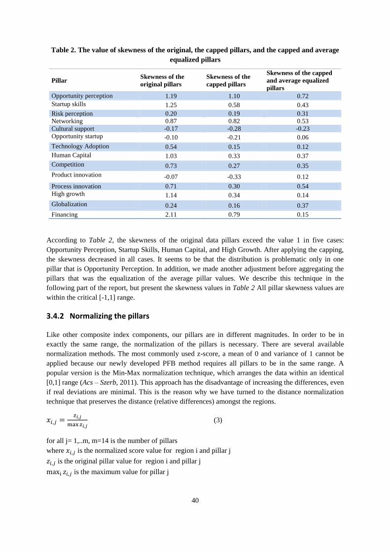
40
Table 2. The value of skewness of the original, the capped pillars, and the capped and average
equalized pillars
Pillar Skewness of the
original pillars
Skewness of the
capped pillars
Skewness of the capped
and average equalized
pillars
Opportunity perception 1.19 1.10 0.72
Startup skills 1.25 0.58 0.43
Risk perception 0.20 0.19 0.31
Networking 0.87 0.82 0.53
Cultural support -0.17 -0.28 -0.23
Opportunity startup -0.10 -0.21 0.06
Technology Adoption 0.54 0.15 0.12
Human Capital 1.03 0.33 0.37
Competition 0.73 0.27 0.35
Product innovation -0.07 -0.33 0.12
Process innovation 0.71 0.30 0.54
High growth 1.14 0.34 0.14
Globalization 0.24 0.16 0.37
Financing 2.11 0.79 0.15
According to Table 2, the skewness of the original data pillars exceed the value 1 in five cases:
Opportunity Perception, Startup Skills, Human Capital, and High Growth. After applying the capping,
the skewness decreased in all cases. It seems to be that the distribution is problematic only in one
pillar that is Opportunity Perception. In addition, we made another adjustment before aggregating the
pillars that was the equalization of the average pillar values. We describe this technique in the
following part of the report, but present the skewness values in Table 2 All pillar skewness values are
within the critical [-1,1] range.
3.4.2 Normalizing the pillars
Like other composite index components, our pillars are in different magnitudes. In order to be in
exactly the same range, the normalization of the pillars is necessary. There are several available
normalization methods. The most commonly used z-score, a mean of 0 and variance of 1 cannot be
applied because our newly developed PFB method requires all pillars to be in the same range. A
popular version is the Min-Max normalization technique, which arranges the data within an identical
[0,1] range (Acs – Szerb, 2011). This approach has the disadvantage of increasing the differences, even
if real deviations are minimal. This is the reason why we have turned to the distance normalization
technique that preserves the distance (relative differences) amongst the regions.
(3)
for all j= 1,..m, m=14 is the number of pillars
where is the normalized score value for region i and pillar j
is the original pillar value for region i and pillar j
is the maximum value for pillar j

41
Applying the distance methodology the pillar values are all in the range [0,1], however the lowest
pillar value is not necessary equal to 0. In this case all regions’ efforts are evaluated in relation to the
benchmarking region but the worst region is not set to zero per se.
3.4.3 Harmonization of the pillars: Equalize pillar averages
The different averages of the normalized values of the 14 pillars imply that reaching the same
performance requires different effort and consequently resources. Higher average values - e.g.
Opportunity startup – could mean that it is easier to reach better scores as compared to lower average
value – e.g. Financing. Since we want to apply REDI for public policy purposes, the additional
resources for the same marginal improvement of the pillar values should be the same for all of the 14
pillars, on the average. So improving by 0.1 unit Opportunity startup should require the same
additional resource as compared to all the other 13 pillars. As a consequence, we need a
transformation to equate the average values of the 14 pillars.
Practically we have calculated the average values of the 14 pillars after the capping adjustment and the
normalization and made the following average adjustment:
Let’s xi to be the normalized score for region i for a particular pillar j.
The arithmetic average of pillar j for number n regions is:
(4)
We want to transform the xi,j values such that the potential values to be in the [0,1] range.
, ,
k
i j i jy x (5)
where k is the “strength of adjustment”, the k th moment of
jX is exactly the needed average, jy .
We have to find the root of the following equation for k :
,
1
0n
k
i j j
i
x ny
(6)
It is easy to see based on previous conditions and derivatives that the function is decreasing and
convex which means it can be quickly solved using the well-known Newton – Raphson method with
an initial guess of 0. After obtaining k, the computations are straightforward. Note that if
1
1
1
j j
j j
j j
x y k
x y k
x y k
that is k be thought of as the strength (and direction) of adjustment.
This technique have resulted the decrease of the over the average value pillars and the increase of the
below the average pillars while keeping the maximum value at 1. Table 3 provides information about
the average pillar values before and after the adjustment.

42
Table 3. Average pillar values before and after the average equalization
Pillar Pillar averages Equalized Pillar
Averages
Opportunity perception 0.38 0.51
Startup skills 0.48 0.51
Risk perception 0.55 0.51
Networking 0.43 0.51
Cultural support 0.52 0.51
Opportunity startup 0.57 0.51
Technology adoption 0.50 0.51
Human capital 0.53 0.51
Competition 0.55 0.51
Product innovation 0.63 0.51
Process innovation 0.59 0.51
High growth 0.44 0.51
Globalization 0.61 0.51
Financing 0.38 0.51
Average 0.51 0.51
While the average of the fourteen pillars is 0.51, it ranges from 0.38 (Opportunity Perception and
Financing) to 0.63 (Process Innovation). It implies that the increase of the REDI scores by, let us say,
10 requires the raise of Financing by approximately 1.66 times more as compared to raise the Process
Innovation. After applying the average equalization adjustment technique the percentage increase of
these two pillars are the same implying a one-to-one substitution of the pillars on the average. A
further consequence of the adjustment that below average value pillars need smaller increase of the
original pillar value to reach the same increase in the REDI points as compared to over the average
pillars. For example, only 0.75 (0.38/0,51) times of the average equalized value of Financing needs to
increase the REDI point by 10, on the average. At the same times, about 1.24 (0,63/0,51) times of the
average equalized value of Process Innovation is required for the same 10 point increase.
3.4.4 The penalty for bottleneck methodology
We have defined entrepreneurship as the dynamic interaction of entrepreneurial attitudes, abilities, and
aspiration across different levels of development. One issue this definition raises is how to bring
system perspective dynamism into the model. Configuration theory provides a useful way of thinking
about this issue (Miller, 1987, 1996). Configurations are defined as “represent[ing] a number of
specific and separate attributes which are meaningful collectively rather than individually.
Configurations are finite in number and represent a unique, tightly integrated, and therefore relatively
long-lived set of dynamics.” (Dess et al., 1993, pp. 775-776.)
Two closely related theories, the Theory of Weakest Link (TWL) and the Theory of Constraints
(TOC), provide us another way to view the interrelationship of the elements. These theories argue that
the performance of the system depends on the element that has the lowest value in the structure.
According to the TOC, improvement can only be achieved by removing the weakest link, which
constrains the performance of the whole system (Goldratt, 1994). The TWL claims that there is no
perfect substitution among the elements of the system, only a partial one Tol and Yohe (2006), Yohe
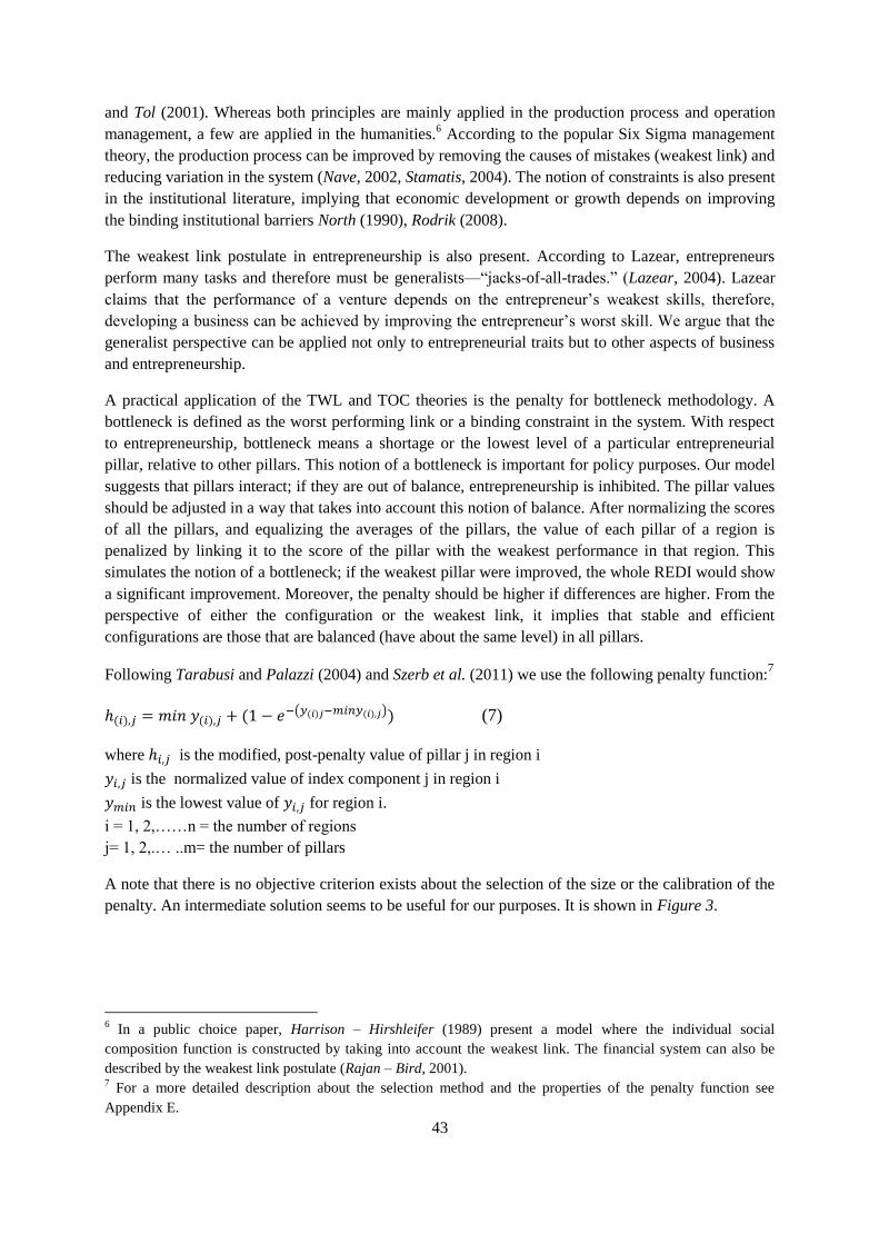
43
and Tol (2001). Whereas both principles are mainly applied in the production process and operation
management, a few are applied in the humanities.6 According to the popular Six Sigma management
theory, the production process can be improved by removing the causes of mistakes (weakest link) and
reducing variation in the system (Nave, 2002, Stamatis, 2004). The notion of constraints is also present
in the institutional literature, implying that economic development or growth depends on improving
the binding institutional barriers North (1990), Rodrik (2008).
The weakest link postulate in entrepreneurship is also present. According to Lazear, entrepreneurs
perform many tasks and therefore must be generalists—“jacks-of-all-trades.” (Lazear, 2004). Lazear
claims that the performance of a venture depends on the entrepreneur’s weakest skills, therefore,
developing a business can be achieved by improving the entrepreneur’s worst skill. We argue that the
generalist perspective can be applied not only to entrepreneurial traits but to other aspects of business
and entrepreneurship.
A practical application of the TWL and TOC theories is the penalty for bottleneck methodology. A
bottleneck is defined as the worst performing link or a binding constraint in the system. With respect
to entrepreneurship, bottleneck means a shortage or the lowest level of a particular entrepreneurial
pillar, relative to other pillars. This notion of a bottleneck is important for policy purposes. Our model
suggests that pillars interact; if they are out of balance, entrepreneurship is inhibited. The pillar values
should be adjusted in a way that takes into account this notion of balance. After normalizing the scores
of all the pillars, and equalizing the averages of the pillars, the value of each pillar of a region is
penalized by linking it to the score of the pillar with the weakest performance in that region. This
simulates the notion of a bottleneck; if the weakest pillar were improved, the whole REDI would show
a significant improvement. Moreover, the penalty should be higher if differences are higher. From the
perspective of either the configuration or the weakest link, it implies that stable and efficient
configurations are those that are balanced (have about the same level) in all pillars.
Following Tarabusi and Palazzi (2004) and Szerb et al. (2011) we use the following penalty function:7
(7)
where is the modified, post-penalty value of pillar j in region i
is the normalized value of index component j in region i
is the lowest value of for region i.
i = 1, 2,……n = the number of regions
j= 1, 2,.… ..m= the number of pillars
A note that there is no objective criterion exists about the selection of the size or the calibration of the
penalty. An intermediate solution seems to be useful for our purposes. It is shown in Figure 3.
6 In a public choice paper, Harrison – Hirshleifer (1989) present a model where the individual social
composition function is constructed by taking into account the weakest link. The financial system can also be
described by the weakest link postulate (Rajan – Bird, 2001). 7 For a more detailed description about the selection method and the properties of the penalty function see
Appendix E.
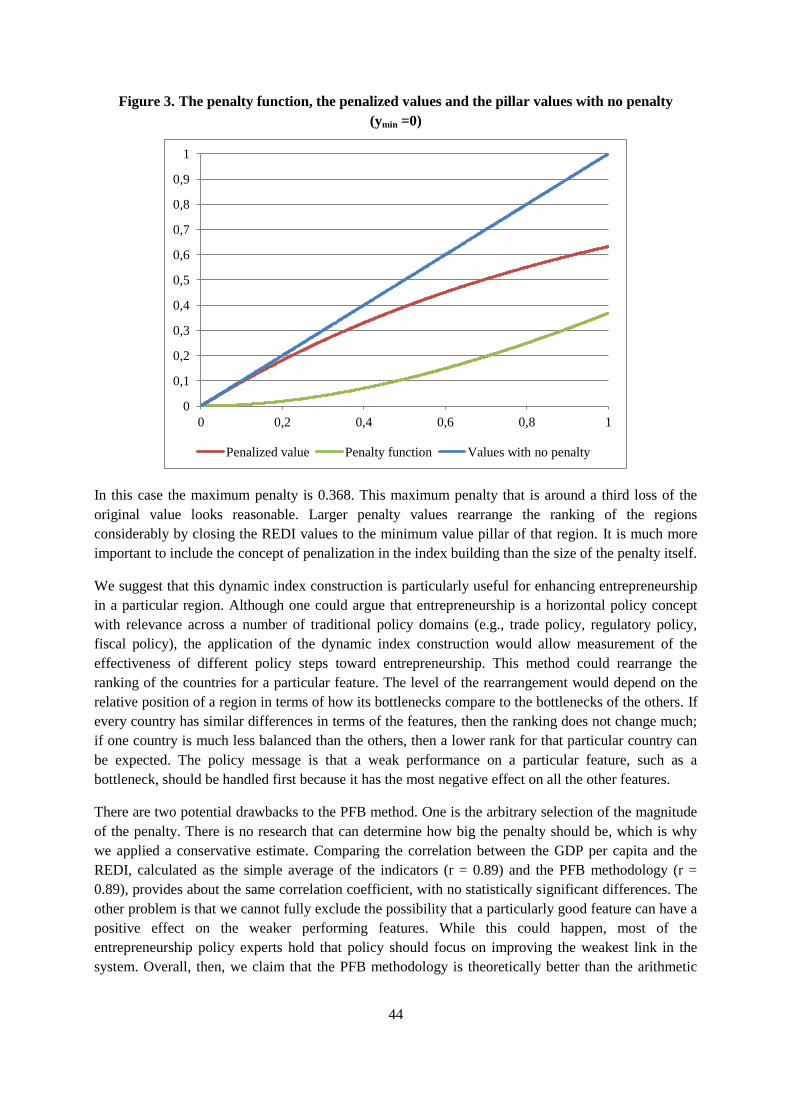
44
Figure 3. The penalty function, the penalized values and the pillar values with no penalty
(ymin =0)
In this case the maximum penalty is 0.368. This maximum penalty that is around a third loss of the
original value looks reasonable. Larger penalty values rearrange the ranking of the regions
considerably by closing the REDI values to the minimum value pillar of that region. It is much more
important to include the concept of penalization in the index building than the size of the penalty itself.
We suggest that this dynamic index construction is particularly useful for enhancing entrepreneurship
in a particular region. Although one could argue that entrepreneurship is a horizontal policy concept
with relevance across a number of traditional policy domains (e.g., trade policy, regulatory policy,
fiscal policy), the application of the dynamic index construction would allow measurement of the
effectiveness of different policy steps toward entrepreneurship. This method could rearrange the
ranking of the countries for a particular feature. The level of the rearrangement would depend on the
relative position of a region in terms of how its bottlenecks compare to the bottlenecks of the others. If
every country has similar differences in terms of the features, then the ranking does not change much;
if one country is much less balanced than the others, then a lower rank for that particular country can
be expected. The policy message is that a weak performance on a particular feature, such as a
bottleneck, should be handled first because it has the most negative effect on all the other features.
There are two potential drawbacks to the PFB method. One is the arbitrary selection of the magnitude
of the penalty. There is no research that can determine how big the penalty should be, which is why
we applied a conservative estimate. Comparing the correlation between the GDP per capita and the
REDI, calculated as the simple average of the indicators (r = 0.89) and the PFB methodology (r =
0.89), provides about the same correlation coefficient, with no statistically significant differences. The
other problem is that we cannot fully exclude the possibility that a particularly good feature can have a
positive effect on the weaker performing features. While this could happen, most of the
entrepreneurship policy experts hold that policy should focus on improving the weakest link in the
system. Overall, then, we claim that the PFB methodology is theoretically better than the arithmetic
0
0,1
0,2
0,3
0,4
0,5
0,6
0,7
0,8
0,9
1
0 0,2 0,4 0,6 0,8 1
Penalized value Penalty function Values with no penalty

45
average calculation. However, the PFB-adjusted REDI is not necessary an optimal solution, since the
magnitude of the penalty is unknown.
3.4.5 Aggregation
The pillars are the basic building blocks of the sub-indices: The entrepreneurial attitudes (ATT), the
entrepreneurial abilities (ABT), and the entrepreneurial aspirations (ASP). The value of a sub-index
for any region is the arithmetic average of its PFB-adjusted pillars for that sub-index multiplied by a
100. The maximum value of the sub-indices is 100 and the potential minimum is 0, both of which
reflect the relative position of a region in a particular sub-index.
(8a)
(8b)
(8c)
where is the modified, post-penalty value of pillar j in region i
i = 1, 2,……n = the number of regions
j= 1, 2,.…..14= the number of pillars
The super-index, the Regional Entrepreneurship and Development Index, is simply the arithmetic
average of the three sub-indices:
(9)
where i = 1, 2,……n = the number of regions
3.4.6 The Average Bottleneck Efficiency (ABE) measure
For measuring the overall level of optimality, we developed the Average Bottleneck Efficiency (ABE)
method. ABE is defined as how close a region’s pillars to a region’s best performing pillar score, on
average. ABE is expressed in terms of percentages. Higher ABE values imply more balanced
performance and therefore more efficient use of the available resources while lower ABE values mean
substantial imbalances over the fourteen pillars of the REDI. An equal alternative indicator of
efficiency is to calculate the Average Bottleneck Gap (ABG). ABG basically shows the percentage of
the wasted resources because of the unbalance of the pillars. ABG also prevails how much additional
resource, on average, is necessary to raise all thirteen pillar values to their maximum pillar value. ABG
is just the opposite to ABE, higher ABG values mean less balanced and low ABG values mean more
balanced performance of the fourteen pillars
Equations 10a and 10b technically describe the general form of the calculation:
(10a)
(10b)
for all j, the number of pillars

46
where ABGi is the Average Bottleneck Gap for region i
where ABEi is the Average Bottleneck Efficiency for region i

47
4 RESULTS AND ANALYSIS
4.1 Introduction
This part of the report is devoted to the interpretation and the analysis of the Regional
Entrepreneurship and Development Index (REDI). As a multi-faceted index, REDI recognizes that
regional level entrepreneurship is a complex phenomenon that cannot be satisfactorily captured by
single-item aggregates, and it cannot be captured by focusing exclusively on attitudes, abilities, or
aspirations. Nor can it be captured by considering the framework conditions alone. What is needed,
therefore, is an approach that combines all of the above. REDI does this by using a total of 14
individual measures of entrepreneurial attitudes, abilities, and aspirations and by weighting them with
descriptors of regional-level framework conditions.
REDI also captures system dynamics and so doing goes beyond traditional, linear-additive index
approaches. Traditional indices are summative – or as we like to call them, ‘cake’ indices: They
simply add different component values together, and as long as the sum of components is greater than
some threshold value, all is considered well. This is similar to if one were advised to compensate for
missing sugar by adding more flour when baking a cake. Although the total weight of ingredients is
the same, everyone recognizes that it is difficult to bake a good cake without sugar.
By applying the Penalty for Bottleneck approach, the REDI index methodology captures the notion
that systems, by definition, comprise multiple components; and that these components co-produce
system performance. These are defining characteristics of any system and ones that simple summative
indices fail to capture. In a simple summative index, each system component contributes directly and
independently to system performance. In the context of entrepreneurship, this would mean that, for
example, a regional measure of education would directly and independent of other system components
contribute to ‘regional entrepreneurship’. In reality, we know that, say, education cannot contribute
much to a region’s entrepreneurial performance, if individuals fail to act. On the other hand, in the
absence of education, the economic potential of entrepreneurial entries would be severely constrained.
Even in the presence of both education and entries into entrepreneurship, regional-level
entrepreneurial performance would be constrained if, e.g., growth aspirations are missing or if there
are no financial resources available to feed the growth of new ventures. A simple summative index
would fail to recognize such interactions – thereby ignoring crucial aspects of system-level
performance.
The system perspective is pictured in Figure 4 where the 14 pillars of the components representing the
three aspects of regional entrepreneurship, attitudes, abilities and aspirations, interact with each other
resulting a Regional Entrepreneurship and Development Index. Unlike most single item
entrepreneurship proxies like self-employment or business density, the REDI measures productive
entrepreneurship that is major source of productivity growth and long term development.
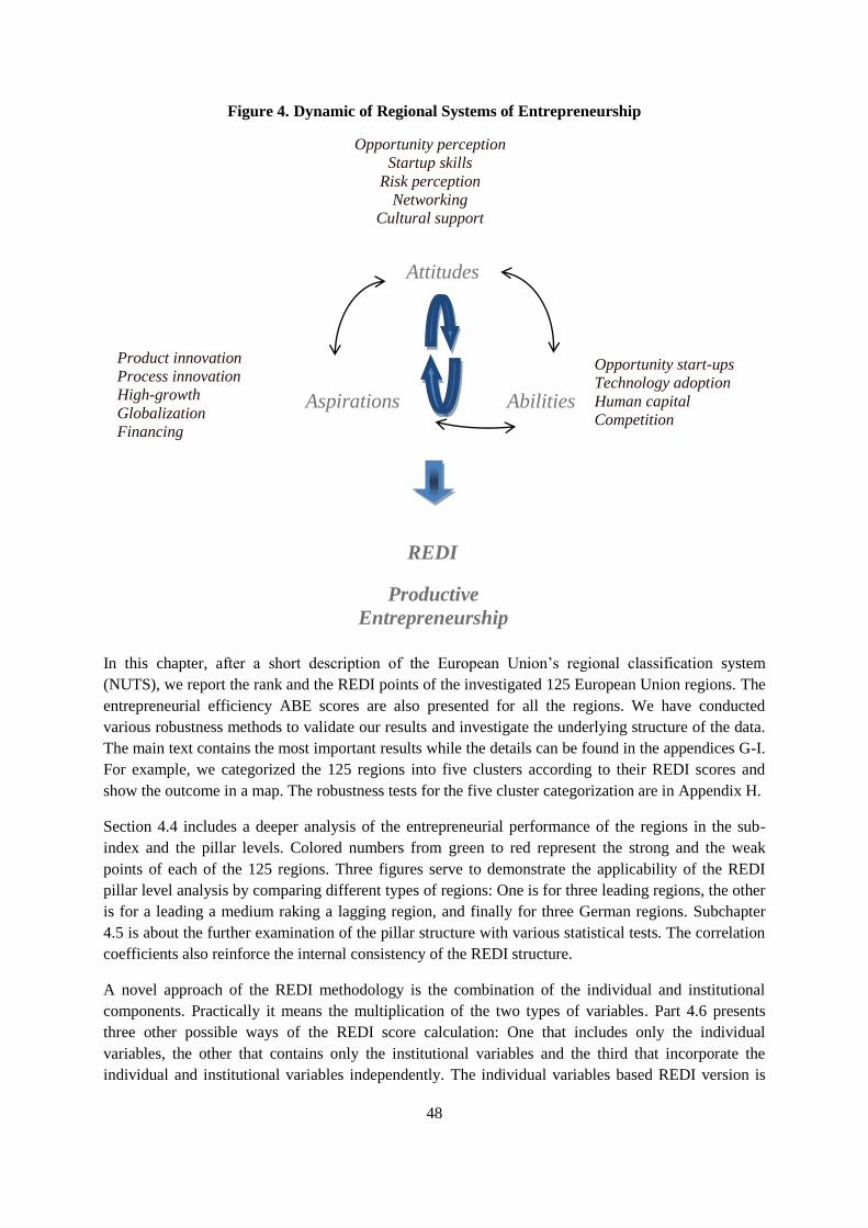
48
Figure 4. Dynamic of Regional Systems of Entrepreneurship
In this chapter, after a short description of the European Union’s regional classification system
(NUTS), we report the rank and the REDI points of the investigated 125 European Union regions. The
entrepreneurial efficiency ABE scores are also presented for all the regions. We have conducted
various robustness methods to validate our results and investigate the underlying structure of the data.
The main text contains the most important results while the details can be found in the appendices G-I.
For example, we categorized the 125 regions into five clusters according to their REDI scores and
show the outcome in a map. The robustness tests for the five cluster categorization are in Appendix H.
Section 4.4 includes a deeper analysis of the entrepreneurial performance of the regions in the sub-
index and the pillar levels. Colored numbers from green to red represent the strong and the weak
points of each of the 125 regions. Three figures serve to demonstrate the applicability of the REDI
pillar level analysis by comparing different types of regions: One is for three leading regions, the other
is for a leading a medium raking a lagging region, and finally for three German regions. Subchapter
4.5 is about the further examination of the pillar structure with various statistical tests. The correlation
coefficients also reinforce the internal consistency of the REDI structure.
A novel approach of the REDI methodology is the combination of the individual and institutional
components. Practically it means the multiplication of the two types of variables. Part 4.6 presents
three other possible ways of the REDI score calculation: One that includes only the individual
variables, the other that contains only the institutional variables and the third that incorporate the
individual and institutional variables independently. The individual variables based REDI version is
Opportunity perception
Startup skills
Risk perception
Networking
Cultural support
Attitudes
Aspirations
Abilities
Opportunity start-ups
Technology adoption
Human capital
Competition
Product innovation
Process innovation
High-growth
Globalization
Financing
REDI
Productive
Entrepreneurship

49
analyzed in details and compared to the original REDI version in the main text. The other two versions
are described in Appendix I.
A common robustness test is to examine the consequences of discarding a pillar and calculating the
new index scores. We provide this type of analysis in 4.7 subchapter by demonstrating the effect on
the change of ranking when we discard each of the pillars one by one. The compensability effects of
the pillars are further examined with the help of the Ordered Weighted Averaging approach. We have
identified 17 regions that were effected the most by the removal of the pillars. Appendix J contains the
effect and the analysis of replacing two institutional variables with other ones. While the REDI scores
and ranks seem to be sensitive for certain changes of the pillars and variables, the magnitude of the
changes are within an acceptable range reinforcing the proper selection of the variables and the
methodology.
In the final subchapter (4.8) the REDI is compared to other regional level indices including the
Regional Competitiveness index, the regional Innovation Scoreboard, the Quality of Government
Index, and the Regional Corruption Index. The close relationship and the high positive correlation
between the REDI and these regional indices is not a surprise since REDI contains several institutional
indicators derived from these indices. Albeit from different perspective, but all of these indices intend
to explain regional development.
4.2 NUTS – Nomenclature of Territorial Units for Statistics
The Nomenclature of Territorial Units for Statistics (hereinafter referred to as NUTS) was developed
at the beginning of the 1970s by the Statistical Office of the European Communities (Eurostat) in close
collaboration with the national statistical institutes of the EU Member States.
The NUTS system can be regarded as a geocode standard for dividing up the whole territory of the
European Union. Currently it is defined only for the 27 Member States of EU. However, Eurostat has
proposed a similar hierarchical classification for countries belong to the European Economic Area
(EEA), Switzerland and the new candidate countries as well.
The main objective of the NUTS system is to ensure a uniform statistical classification of the
territorial units of the EU Member States in order to collect, compile and disseminate comparable,
harmonized regional statistics primarily for conducting socio-economic analyses. A decisive role of
the NUTS system is to minimize the impact of fortuitous changes in the national administrative
structures of different EU countries. However, the NUTS classification has been changed several times
starting from 1981 to reflect the administrative changes of the Member States. All Member States'
spatial statistics has been delivered to the European Commission should use the NUTS classification.
Furthermore, the hierarchical system of the NUTS nomenclature was developed for framing EU
regional policies and it has a direct role of appraising eligibility for financial support from the EU
Structural Fund.
Two criteria are used in subdividing the territory of the Member States into spatial units:
“normative regions are the expression of political will; their limits are fixed according to the tasks
allocated to the territorial communities, according to the sizes of population necessary to carry out
these tasks efficiently and economically, and according to historical, cultural and other factors;
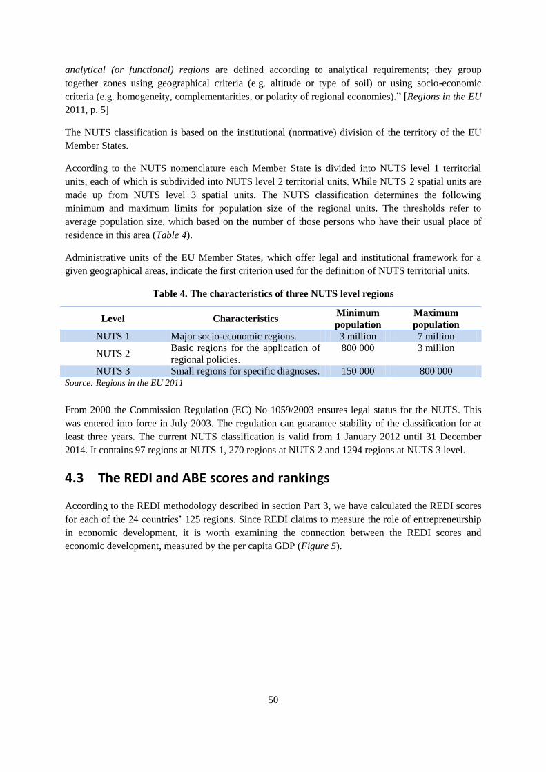
50
analytical (or functional) regions are defined according to analytical requirements; they group
together zones using geographical criteria (e.g. altitude or type of soil) or using socio-economic
criteria (e.g. homogeneity, complementarities, or polarity of regional economies).” [Regions in the EU
2011, p. 5]
The NUTS classification is based on the institutional (normative) division of the territory of the EU
Member States.
According to the NUTS nomenclature each Member State is divided into NUTS level 1 territorial
units, each of which is subdivided into NUTS level 2 territorial units. While NUTS 2 spatial units are
made up from NUTS level 3 spatial units. The NUTS classification determines the following
minimum and maximum limits for population size of the regional units. The thresholds refer to
average population size, which based on the number of those persons who have their usual place of
residence in this area (Table 4).
Administrative units of the EU Member States, which offer legal and institutional framework for a
given geographical areas, indicate the first criterion used for the definition of NUTS territorial units.
Table 4. The characteristics of three NUTS level regions
Level Characteristics Minimum
population
Maximum
population
NUTS 1 Major socio-economic regions. 3 million 7 million
NUTS 2 Basic regions for the application of
regional policies.
800 000 3 million
NUTS 3 Small regions for specific diagnoses. 150 000 800 000 Source: Regions in the EU 2011
From 2000 the Commission Regulation (EC) No 1059/2003 ensures legal status for the NUTS. This
was entered into force in July 2003. The regulation can guarantee stability of the classification for at
least three years. The current NUTS classification is valid from 1 January 2012 until 31 December
2014. It contains 97 regions at NUTS 1, 270 regions at NUTS 2 and 1294 regions at NUTS 3 level.
4.3 The REDI and ABE scores and rankings
According to the REDI methodology described in section Part 3, we have calculated the REDI scores
for each of the 24 countries’ 125 regions. Since REDI claims to measure the role of entrepreneurship
in economic development, it is worth examining the connection between the REDI scores and
economic development, measured by the per capita GDP (Figure 5).
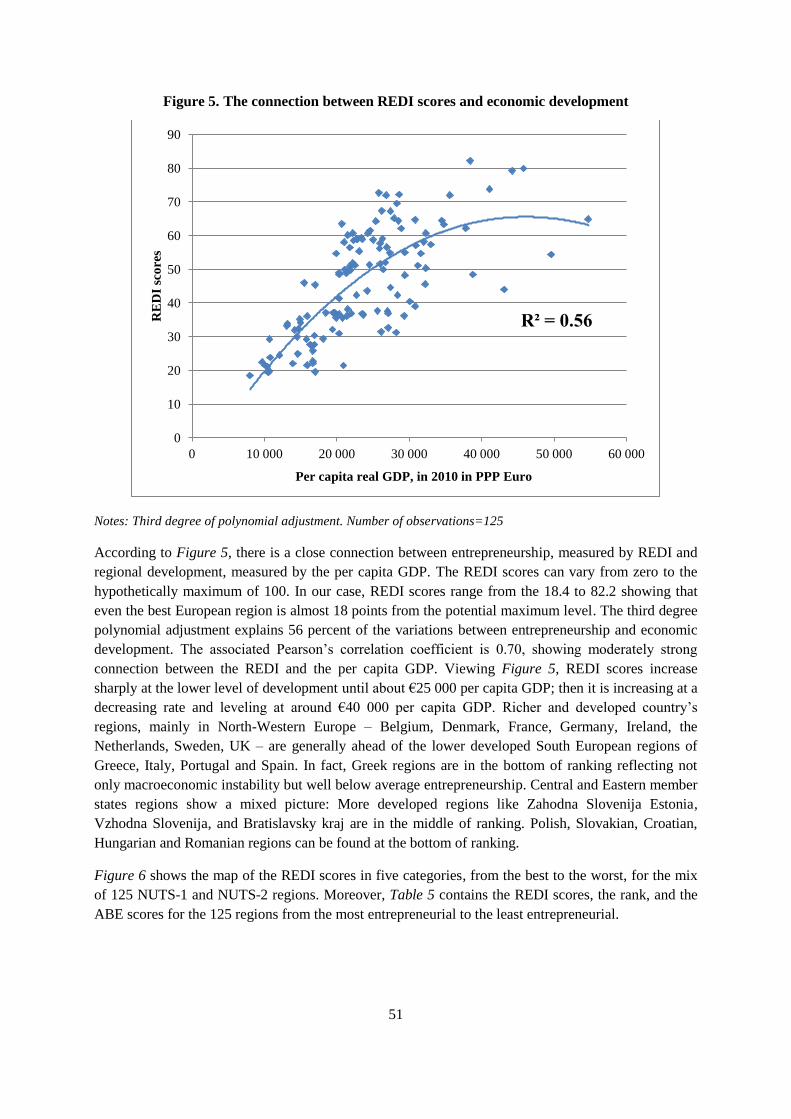
51
Figure 5. The connection between REDI scores and economic development
Notes: Third degree of polynomial adjustment. Number of observations=125
According to Figure 5, there is a close connection between entrepreneurship, measured by REDI and
regional development, measured by the per capita GDP. The REDI scores can vary from zero to the
hypothetically maximum of 100. In our case, REDI scores range from the 18.4 to 82.2 showing that
even the best European region is almost 18 points from the potential maximum level. The third degree
polynomial adjustment explains 56 percent of the variations between entrepreneurship and economic
development. The associated Pearson’s correlation coefficient is 0.70, showing moderately strong
connection between the REDI and the per capita GDP. Viewing Figure 5, REDI scores increase
sharply at the lower level of development until about €25 000 per capita GDP; then it is increasing at a
decreasing rate and leveling at around €40 000 per capita GDP. Richer and developed country’s
regions, mainly in North-Western Europe – Belgium, Denmark, France, Germany, Ireland, the
Netherlands, Sweden, UK – are generally ahead of the lower developed South European regions of
Greece, Italy, Portugal and Spain. In fact, Greek regions are in the bottom of ranking reflecting not
only macroeconomic instability but well below average entrepreneurship. Central and Eastern member
states regions show a mixed picture: More developed regions like Zahodna Slovenija Estonia,
Vzhodna Slovenija, and Bratislavsky kraj are in the middle of ranking. Polish, Slovakian, Croatian,
Hungarian and Romanian regions can be found at the bottom of ranking.
Figure 6 shows the map of the REDI scores in five categories, from the best to the worst, for the mix
of 125 NUTS-1 and NUTS-2 regions. Moreover, Table 5 contains the REDI scores, the rank, and the
ABE scores for the 125 regions from the most entrepreneurial to the least entrepreneurial.
R² = 0.56
0
10
20
30
40
50
60
70
80
90
0 10 000 20 000 30 000 40 000 50 000 60 000
RE
DI
sco
res
Per capita real GDP, in 2010 in PPP Euro

52
Figure 6. The map of REDI scores in five cluster categories in 125 European Union regions, 2013

53
Table 5. The REDI ranking, REDI scores, and the ABE scores of the 125 European Union regions
Rank Code Region REDI ABE Rank Code Region REDI ABE Rank Code Region REDI ABE
1 DK01 Hovedstaden 82.2 90.2 42 UKF East Midlands (UK) 55.3 64.8 83 ES41 Castilla y León 36.8 66.4
2 UKI London 79.9 85.3 43 DEA Nordrhein-Westfalen 55.0 69.8 84 ES62 Región de Murcia 36.7 64.0
3 FR1 Île de France 79.2 84.5 44 DEC Saarland 54.9 69.4 85 ES13 Cantabria 36.5 55.0
4 SE11 Stockholm 73.8 84.4 45-46 UKL Wales 54.7 64.2 86-88 ITH Nord-Est 36.1 65.2
5 SE12 Östra Mellansverige 72.7 78.3 45-46 ES30 Comunidad de Madrid 54.7 64.8 86-88 PL5
Region Poludniowo-
Zachodni 36.1 54.7
6 SE23 Vastsverige 72.2 78.3 47 DE6 Hamburg 54.3 69.6 86-88 PL1 Region Centralny 36.1 53.4
7-8 IE02 Southern and Eastern 72.0 78.1 48 AT2 Südösterreich 52.0 61.5 89 DE8 Mecklenburg-Vorpommern 35.6 61.9
7-8 DK05 Nordjylland 72.0 83.1 49 FR5 Ouest (FR) 51.8 70.4 90 ES70 Canarias (ES) 35.5 62.6
9 UKJ South East (UK) 69.5 76.9 50 DE9 Niedersachsen 51.6 70.3 91 LT Lithuania 35.2 47.9
10 SE22 Sydsverige 67.3 78.2 51 SI02 Zahodna Slovenija 51.3 68.6 92 PL2 Region Poludniowy 34.1 59.6
11 DE3 Berlin 67.2 77.3 52 FI1D Pohjois- ja Ita-Suomi 51.2 66.7 93 LV Latvia 33.8 51.3
12 DK03 Syddanmark 65.1 76.4 53 NL1 Noord-Nederland 51.1 62.0 94 PL6 Region Pólnocny 33.2 64.2
13 BE1
Région de Bruxelles-
Capitale 64.9 77.2 54 FR2 Bassin Parisien 50.9 67.0 95 ES24 Aragón 32.6 55.9
14 SE33 Övre Norrland 64.7 75.4 55 AT3 Westösterreich 50.3 61.7 96 PL4 Region Pólnocno-Zachodni 32.3 62.1
15 NL3 West-Nederland 64.4 79.3 56 DED Sachsen 50.0 72.1 97 ES42 Castilla-la Mancha 32.1 58.3
16 DK04 Midtjylland 64.3 78.8 57 SE21 Smaland med öarna 49.9 62.3 98 HR03
Jadranska Hrvatska (Adriatic
Croatia) 32.0 53.0
17 FR7 Centre-Est (FR) 64.2 74.6 58 FR4 Est (FR) 49.7 70.3 99 HU10 Közép-Magyarország 31.4 50.2
18 IE01
Border. Midland and
Western 63.4 74.1 59 UKC North East (UK) 48.9 64.4 100 EL3 Attiki 31.3 63.7
19 DE7 Hessen 63.3 73.1 60 FR3 Nord - Pas-de-Calais 48.8 64.7 101 PT15 Algarve 30.9 46.6
20 FI1B Helsinki-Uusimaa 62.2 75.3 61 DE4 Brandenburg 48.5 68.4 102 ES43 Extremadura 30.3 56.2
21 BE2 Vlaams Gewest 62.1 76.2 62 DE5 Bremen 48.4 67.5 103 HR04
Kontinentalna Hrvatska
(Continental Croatia) 29.9 51.1
22 UKH East of England 61.5 71.4 63 SE32 Mellersta Norrland 48.2 68.5 104 PT18 Alentejo 29.4 46.4
23-25 DK02 Sjalland 60.7 79.5 64 EE Estonia 45.9 64.5 105-106 PL3 Region Wschodni 29.2 46.8
23-25 UKK South West (UK) 60.7 68.7 65 ES21 País Vasco 45.6 57.3 105-106 PT11 Norte 29.2 55.3
23-25 AT1 Ostösterreich 60.7 70.4 66 SI01 Vzhodna Slovenija 45.3 78.9 107-108 PT16 Centro (PT) 27.6 45.5
26 BE3 Région wallonne 60.1 69.9 67 PT17 Lisboa 44.6 69.4 107-108 ITG Isole 27.6 57.5
27 FR8 Méditerranée 59.4 67.0 68 SK01 Bratislavsky kraj 44.0 64.3 109 ITF Sud 27.3 55.6

54
Rank Code Region REDI ABE Rank Code Region REDI ABE Rank Code Region REDI ABE
28-29 UKD North West (UK) 59.0 69.4 69 DEF Schleswig-Holstein 43.6 63.0 110 SK02 Západné Slovensko 25.8 36.0
28-29 UKM Scotland 59.0 69.2 70-72 ES12 Principado de Asturias 42.3 63.2 111 SK03 Stredné Slovensko 24.9 50.3
30-31 FI1C Etelä-Suomi 58.9 73.0 70-72 ES51 Cataluna 42.3 70.4 112 SK04 Vychodné Slovensko 24.5 42.1
30-31 FR6 Sud-Ouest (FR) 58.9 69.4 70-72 DEE Sachsen-Anhalt 41.3 61.7 113 HU23 Dél-Dunántúl 23.8 50.0
32 FI19 Länsi-Suomi 58.7 74.9 73 ITC Nord-Ovest 40.4 72.0 114 EL1 Voreia Ellada 22.7 48.4
33 UKG West Midlands (UK) 58.6 67.3 74 ES22
Comunidad Foral de
Navarra 39.0 49.5 115 HU31 Észak-Magyarország 22.4 28.9
34 DE1 Baden-Württemberg 58.1 77.4 75 ES52
Comunidad
Valenciana 38.1 67.1 116 RO3 Macroregiunea trei 22.1 37.3
35 UKN Northern Ireland (UK) 58.0 70.5 76 ES53 Illes Balears 37.7 56.6 117 HU21 Közép-Dunántúl 22.0 43.6
36 SE31 Norra Mellansverige 57.7 69.0 77 ES23 La Rioja 37.6 56.0 118 HU22 Nyugat-Dunántúl 21.5 55.1
37 DE2 Bayern 57.3 75.8 78 DEG Thüringen 37.2 61.5 119-120 HU32 Észak-Alföld 21.4 52.9
38 NL4 Zuid-Nederland 57.0 70.8 79 ES61 Andalucía 37.1 68.0 119-120 EL4 Nisia Aigaiou. Kriti 21.4 39.7
39 NL2 Oost-Nederland 56.5 72.0 80 CZ Czech Republic 37.0 49.1 121 HU33 Dél-Alföld 21.0 55.5
40 UKE Yorkshire and The Humber 56.4 65.9 81-82 ITI Centro (IT) 36.9 57.5 122 RO4 Macroregiunea patru 19.7 31.2
41 DEB Rheinland-Pfalz 56.2 70.1 81-82 ES11 Galicia 36.9 61.8 123 EL2 Kentriki Ellada 19.5 38.1
124-125 RO1 Macroregiunea unu 19.4 31.3
124-125 RO2 Macroregiunea doi 18.4 28.9

55
Table 5 shows the rank and the REDI points of the 125 regions from the lowest to the highest. As
expected, the variations in entrepreneurship over the 125 regions are substantial, over four-fold
between the 1st Hovedstaden and the 125
th Romanian Macroregiunea doi. It means that Hovedstaden
has reached 82.2 points out of the maximum reachable 100 points. At the same time, Macroregiunea
doi has achieved only 18.4 points. In the first ten regions, four Swedish, two Danish, two United
Kingdom, one French, and one Irish region can be found. According to our calculation, the Danish
Hovedstaden, with Copenhagen in the center, is found to be the most entrepreneurial region in the
European Union. The EUs two mostly agglomerated regions, London and Íle de France rank 2nd
and
3rd
, respectively. Larger, more developed city regions with higher per capita GDP generally rank ahead
of lower developed regions in the same countries. Most of the times capital cities, that are generally
the largest and the most developed, lead the country rank. There are two exceptions: The best Dutch
region is West Netherland with Amsterdam, and the Milan centered Nord-Ovest region is leading in
Italy. Two Polish regions, Region Poludniowo-Zachodni and Region Centraly including Warsaw have
exactly the same REDI points, 36.1.
We conducted a K-means cluster analysis taking into account only the REDI score values. For our
purposes the five group version proved to be the best. According to the ANOVA test, the differences
between any two of the REDI groups are smaller than within the groups, at p=0.001 level. A more
detailed robustness analysis about the selection of the five clusters can be found in Appendix H.
Figure 6 shows the cluster membership of all the 125 regions. Nine regions from 82.2 to 69.5 REDI
points belong to the best cohort. These are mainly Nordic country regions. 32 regions, from the 10th to
the 41st place, constitute the second group of regions. Their REDI scores range from 67.3 to 56.2.
Besides the remaining of the Nordic country regions, United Kingdom, Belgian, Dutch and some
French as well as the best German regions can be found here. The following 28 regions the UK East
Midlands (55.3 REDI points, 42nd
place) to the German Schleswig-Holstein (43.6 REDI points, 69th
place) form the third group. Most Austrian, German and French regions form this cluster together with
the best Central- and South European regions. The most populous is the fourth group with 37 regions
ranging from the 70-72nd
place to the 105-106th place. Their REDI scores are much lower, 42.3-29.2
REDI scores. Mainly former East German, Spanish, Italian, Polish and Croatian regions make up this
cluster. The last group of regions is mainly from Greece, Hungary, Portugal Slovakia and Romani
together with two Italian regions. They occupy the 107-125th places with 27.6-18.4 REDI scores..
The Average Bottleneck Efficiency (ABE) measure reflects to the use of available resources. High
ABE score mean that a particular region uses its available resource efficiently. It also implies that the
fourteen pillars of the REDI are very close to each other without significant bottleneck. Because of the
use of the PFB methodology it is not possible to reach good scores with unbalanced performance. On
the contrary, it is possible to have low REDI points and high ABE scores, at least in theory. It could
indicate that a region use efficiently its limited entrepreneurial resources. However, practically the
REDI and the ABE scores correlate closely (Figure 7).

56
Figure 7. The connection between the REDI and the ABE scores
Notes: Third degree of polynomial adjustment. Number of observations=125
The third degree polynomial curve explains 83% of the total variation between REDI and ABE.
Figure 7 also prevails that the ABE score variations are higher in the lower and relatively low at the
higher levels. Hovedstaden, the leading Danish region has the highest ABE scores of 90.2% implying
that less than 10 percent of its available entrepreneurial resources are wasted more or less. The first ten
regions’ ABE scores exceed the 78% with the exception of the UK South-East region that has a little
bit less ABE score (76.9%). In the middle of ranking, the 66th Slovenian Vzhodna Slovenija has only a
moderate 45.3 REDI point but possesses a relatively high 78.9 ABE score. It seems that UK regions,
except the second ranked London have the tendency to have lower ABE scores than implied by their
REDI points. At the bottom of ranking we can find ABE scores around 30%. The Romanian
Macroregiunea doi is not only the last in the ranking but has the lowest ABE score of 28.9% together
with the 115th ranked Hungarian Észak-Magyarország. At the same time another Hungarian region, the
121st Dél-Alföld’s ABE score is 55.5; much higher that we would have expected according to its 21.4
REDI point.
4.4 The analysis of the three sub-indices and the fourteen pillars
While the REDI points are suitable to compare the overall entrepreneurial performances of the regions
they are not proper for policy application. The REDI needs to be decomposed to be able to get a more
accurate picture about the entrepreneurial profile of the regions and the potential direction of
entrepreneurship policy action. Table 6 provides the scores and the ranking of the 125 regions in all
three sub-indices.
R² = 0.83
0
10
20
30
40
50
60
70
80
90
100
0 10 20 30 40 50 60 70 80 90
AB
E p
oin
ts
REDI scores

57
Table 6. The Entrepreneurial Attitudes (ATT), Entrepreneurial Abilities (ABT) and Entrepreneurial Aspirations (ASP) values and ranks of the 125
regions
Regional
Code Region ATT
ATT
Rank ABT
ABT
Rank ASP
ASP
Rank
Regional
Code Region ATT
ATT
Rank ABT
ABT
Rank ASP
ASP
Rank
AT1 Ostösterreich 58.8 33 60.4 35 62.8 14 HR03
Jadranska Hrvatska
(Adriatic Croatia) 24.1 107 27.4 96 44.4 68
AT2 Südösterreich 50.2 52 49 62 56.7 31 HR04
Kontinentalna Hrvatska
(Continental Croatia) 23.1 108 26.6 97 40 76
AT3 Westösterreich 51.6 50 45.9 66 53.3 40 HU10 Közép-Magyarország 30.2 102 31.8 93 32.1 101
BE1
Région de Bruxelles-
Capitale 61.1 30 63.6 27 69.9 8 HU21 Közép-Dunántúl 20.7 116 23.9 101 21.3 123
BE2 Vlaams Gewest 55.4 41 68.5 14 62.5 16 HU22 Nyugat-Dunántúl 21.4 113 25.4 98 17.7 125
BE3 Région wallonne 52.1 48 57.2 43 71.1 5 HU23 Dél-Dunántúl 22.2 109 24.2 100 25 117
CZ Czech Republic 29.5 104 21.5 107 60.1 24 HU31 Észak-Magyarország 19.3 122 24.3 99 23.6 118
DE1 Baden-Württemberg 54 44 60.4 36 59.9 25 HU32 Észak-Alföld 20 119 23.4 104 20.9 124
DE2 Bayern 51.9 49 59.4 38 60.6 21 HU33 Dél-Alföld 20 120 20.1 109 23 120
DE3 Berlin 57.5 37 74.4 9 69.7 9 IE01
Border. Midland and
Western 66.8 20 63.9 26 59.6 26
DE4 Brandenburg 41.3 69 55.9 48 48.3 50 IE02 Southern and Eastern 72.8 8 76.9 7 66.2 11
DE5 Bremen 46.7 58 52.2 55 46.4 62 ITC Nord-Ovest 38.5 76 35.8 84 46.8 59
DE6 Hamburg 56.3 39 65.3 23 41.4 73 ITF Sud 29.4 105 20.3 108 32.2 100
DE7 Hessen 53.5 45 66.4 19 69.9 7 ITG Isole 29.5 103 22.2 106 31.1 104
DE8
Mecklenburg-
Vorpommern 38.5 77 35.1 87 33.2 98 ITH Nord-Est 37.5 83 34.7 88 36.3 87
DE9 Niedersachsen 46.1 60 52 57 56.6 32 ITI Centro (IT) 37 88 31.9 92 42 72
DEA Nordrhein-Westfalen 52.4 47 54.6 52 57.9 27 LT Lithuania 35.6 91 33.5 90 36.6 86
DEB Rheinland-Pfalz 49.6 53 55.3 49 63.7 13 LV Latvia 34.3 95 31.5 94 35.6 90
DEC Saarland 47.7 57 55.9 47 61 19 NL1 Noord-Nederland 55.7 40 50 59 47.6 54
DED Sachsen 45.5 63 58.4 42 46.1 64 NL2 Oost-Nederland 60.4 31 54.8 51 54.3 36
DEE Sachsen-Anhalt 39.7 73 42.1 73 42.2 71 NL3 West-Nederland 66.9 19 65.4 22 61 20
DEF Schleswig-Holstein 42.9 67 48.8 63 38.9 79 NL4 Zuid-Nederland 61.1 29 57.1 44 52.9 41
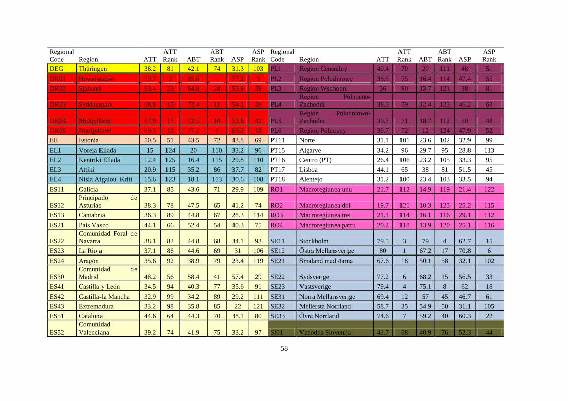
58
Regional
Code Region ATT
ATT
Rank ABT
ABT
Rank ASP
ASP
Rank
Regional
Code Region ATT
ATT
Rank ABT
ABT
Rank ASP
ASP
Rank
DEG Thüringen 38.2 81 42.1 74 31.3 103 PL1 Region Centralny 40.4 70 20 111 48 51
DK01 Hovedstaden 79.7 2 89.6 1 77.2 3 PL2 Region Poludniowy 38.5 75 16.4 114 47.4 55
DK02 Sjalland 63.4 23 64.8 24 53.9 39 PL3 Region Wschodni 36 90 13.7 121 38 81
DK03 Syddanmark 68.8 15 72.4 11 54.1 38 PL4
Region Pólnocno-
Zachodni 38.3 79 12.4 123 46.2 63
DK04 Midtjylland 67.9 17 72.5 10 52.6 42 PL5
Region Poludniowo-
Zachodni 39.7 71 18.7 112 50 48
DK05 Nordjylland 69.5 11 77.2 6 69.2 10 PL6 Region Pólnocny 39.7 72 12 124 47.9 52
EE Estonia 50.5 51 43.5 72 43.8 69 PT11 Norte 31.1 101 23.6 102 32.9 99
EL1 Voreia Ellada 15 124 20 110 33.2 96 PT15 Algarve 34.2 96 29.7 95 28.8 113
EL2 Kentriki Ellada 12.4 125 16.4 115 29.8 110 PT16 Centro (PT) 26.4 106 23.2 105 33.3 95
EL3 Attiki 20.9 115 35.2 86 37.7 82 PT17 Lisboa 44.1 65 38 81 51.5 45
EL4 Nisia Aigaiou. Kriti 15.6 123 18.1 113 30.6 108 PT18 Alentejo 31.2 100 23.4 103 33.5 94
ES11 Galicia 37.1 85 43.6 71 29.9 109 RO1 Macroregiunea unu 21.7 112 14.9 119 21.4 122
ES12
Principado de
Asturias 38.3 78 47.5 65 41.2 74 RO2 Macroregiunea doi 19.7 121 10.3 125 25.2 115
ES13 Cantabria 36.3 89 44.8 67 28.3 114 RO3 Macroregiunea trei 21.1 114 16.1 116 29.1 112
ES21 País Vasco 44.1 66 52.4 54 40.3 75 RO4 Macroregiunea patru 20.2 118 13.9 120 25.1 116
ES22
Comunidad Foral de
Navarra 38.1 82 44.8 68 34.1 93 SE11 Stockholm 79.5 3 79 4 62.7 15
ES23 La Rioja 37.1 86 44.6 69 31 106 SE12 Östra Mellansverige 80 1 67.2 17 70.8 6
ES24 Aragón 35.6 92 38.9 79 23.4 119 SE21 Smaland med öarna 67.6 18 50.1 58 32.1 102
ES30
Comunidad de
Madrid 48.2 56 58.4 41 57.4 29 SE22 Sydsverige 77.2 6 68.2 15 56.5 33
ES41 Castilla y León 34.5 94 40.3 77 35.6 91 SE23 Vastsverige 79.4 4 75.1 8 62 18
ES42 Castilla-la Mancha 32.9 99 34.2 89 29.2 111 SE31 Norra Mellansverige 69.4 12 57 45 46.7 61
ES43 Extremadura 33.2 98 35.8 85 22 121 SE32 Mellersta Norrland 58.7 35 54.9 50 31.1 105
ES51 Cataluna 44.6 64 44.3 70 38.1 80 SE33 Övre Norrland 74.6 7 59.2 40 60.3 22
ES52
Comunidad
Valenciana 39.2 74 41.9 75 33.2 97 SI01 Vzhodna Slovenija 42.7 68 40.9 76 52.3 44
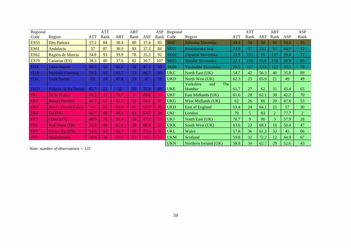
59
Regional
Code Region ATT
ATT
Rank ABT
ABT
Rank ASP
ASP
Rank
Regional
Code Region ATT
ATT
Rank ABT
ABT
Rank ASP
ASP
Rank
ES53 Illes Balears 37.2 84 38.4 80 37.4 83 SI02 Zahodna Slovenija 49.4 54 50 60 54.4 35
ES61 Andalucía 37 87 36.9 83 37.3 84 SK01 Bratislavsky kraj 33.9 97 33.1 91 64.9 12
ES62 Región de Murcia 34.8 93 39.9 78 35.3 92 SK02 Západné Slovensko 21.9 111 16 117 39.4 77
ES70 Canarias (ES) 38.3 80 37.6 82 30.7 107 SK03 Stredné Slovensko 22.1 110 15.6 118 36.9 85
FI19 Länsi-Suomi 68.3 16 60.5 34 47.2 56 SK04 Vychodné Slovensko 20.5 117 13.6 122 39.3 78
FI1B Helsinki-Uusimaa 70.5 10 69.2 13 46.7 60 UKC North East (UK) 54.7 42 56.3 46 35.8 89
FI1C Etelä-Suomi 69 14 60.8 33 47 58 UKD North West (UK) 62.3 25 65.9 21 49 49
FI1D Pohjois- ja Ita-Suomi 65.7 21 52 56 35.9 88 UKE
Yorkshire and The
Humber 61.7 27 62 31 45.4 65
FR1 Île de France 69.3 13 78.7 5 89.6 1 UKF East Midlands (UK) 61.6 28 62.1 30 42.2 70
FR2 Bassin Parisien 45.7 62 52.7 53 54.2 37 UKG West Midlands (UK) 62 26 66 20 47.6 53
FR3 Nord - Pas-de-Calais 46 61 49.8 61 50.7 46 UKH East of England 63.4 24 64.1 25 57 30
FR4 Est (FR) 46.7 59 48.1 64 54.5 34 UKI London 79 5 83 2 77.7 2
FR5 Ouest (FR) 48.9 55 59.4 39 47.2 57 UKJ South East (UK) 70.7 9 80 3 57.9 28
FR6 Sud-Ouest (FR) 53.5 46 62.8 28 60.3 23 UKK South West (UK) 63.6 22 68.1 16 50.4 47
FR7 Centre-Est (FR) 54.6 43 66.7 18 71.4 4 UKL Wales 57.8 36 61.2 32 45 66
FR8 Méditerranée 56.6 38 59.5 37 62 17 UKM Scotland 59.8 32 72.2 12 44.9 67
UKN Northern Ireland (UK) 58.8 34 62.7 29 52.6 43
Note: number of observations = 125

62
The examination of the three sub-indexes demonstrates the varieties of the regions entrepreneurial
characteristics. There are only a few well balanced regions exists, e.g. London is one of these with
77.7 ASP, 79.0 ATT and 83.0 ABT values. Stockholm is at the fourth place in the REDI ranking. A
closer look at its sub-indices prevails a high ATT score (79.5), a little bit lower ASP value (79.0) but
its ASP score is relatively low “only” 62.7. Picking up a Spanish region, Galicia, has a relatively high
ABT score (43.6), an acceptable ATT score (37.1) but a very low ASP score (29.9). Most Polish
regions seem to have a relatively low performance in ASP. While Hungarian and Romanian regions
are at the bottom of ranking, their three sub-indices are relatively well-balanced at the low level.
An analysis on the 14 pillar level provides a more detailed and a more precise picture about the
entrepreneurial profile of a region. Table 7 shows the non-penalized average equated pillar values for
all the 125 regions. The colors help to identify the position of a region’s particular pillar. For example,
Noord-Nederland has a maximum value in Cultural support (green color) but weaker in Competition
(0.52, amber color) and low in Risk perception (0.29, reddish color). Greener colors mean higher and
better scores while reddish color imply poor performance that may call for policy intervention.

63
Table 7. The fourteen average equated pillar values of the 125 European Union regions R
egio
na
l C
od
e
Reg
ion
s
Op
po
rtu
nit
y
per
cep
tio
n
Str
at-
up
sk
ills
Ris
k P
erce
pti
on
Net
wo
rkin
g
Cu
ltu
ral
sup
po
rt
Op
po
rtu
nit
y
sta
rtu
p
Tec
hn
olo
gy
Ab
sorp
tio
n
Hu
ma
n C
ap
ita
l
Co
mp
etit
ion
Pro
du
ct
inn
ov
ati
on
Pro
cess
in
no
va
tio
n
Hig
h g
row
th
Glo
ba
liza
tio
n
Fin
an
cin
g
AT1 Ostösterreich 0.77 0.86 0.40 0.65 0.48 0.63 0.72 0.40 0.84 0.78 0.53 0.37 0.79 1.00
AT2 Südösterreich 0.41 0.73 0.41 0.57 0.52 0.58 0.68 0.32 0.49 0.58 0.52 0.39 0.64 1.00
AT3 Westösterreich 0.54 0.72 0.42 0.61 0.51 0.60 0.44 0.26 0.67 0.58 0.41 0.32 0.71 1.00
BE1 Région de
Bruxelles-Capitale 0.76 0.86 0.90 0.50 0.37 0.34 1.00 1.00 0.58 0.97 0.50 1.00 0.97 0.60
BE2 Vlaams Gewest 0.46 0.64 0.86 0.44 0.47 0.82 0.61 0.73 0.77 0.42 0.73 0.49 0.89 0.81
BE3 Région wallonne 0.46 0.66 0.79 0.42 0.39 0.47 0.57 0.68 0.66 0.57 0.98 0.75 0.97 0.68
CZ Czech Republic 0.52 0.38 0.15 0.29 0.23 0.20 0.28 0.16 0.24 0.62 1.00 0.86 0.97 0.43
DE1 Baden-
Württemberg 0.55 0.64 0.39 0.55 0.66 0.73 0.66 0.46 0.71 0.74 0.41 0.62 0.59 0.81
DE2 Bayern 0.45 0.60 0.37 0.60 0.66 0.61 0.74 0.49 0.67 0.49 0.42 0.77 0.75 0.83
DE3 Berlin 0.78 0.73 0.39 0.57 0.56 0.66 0.90 0.79 1.00 0.89 0.40 0.82 0.87 0.90
DE4 Brandenburg 0.33 0.73 0.37 0.51 0.55 0.54 0.69 0.77 1.00 0.61 0.07 1.00 0.97 0.64
DE5 Bremen 0.56 0.57 0.39 0.74 0.58 0.50 0.53 0.99 0.65 1.00 0.37 0.09 0.97 0.66
DE6 Hamburg 0.94 0.81 0.42 0.67 0.52 0.80 1.00 0.52 1.00 0.69 0.27 0.19 0.50 0.67
DE7 Hessen 0.62 0.62 0.38 0.57 0.59 0.54 0.66 0.73 0.99 0.77 0.53 1.00 0.88 0.72
DE8 Mecklenburg-
Vorpommern 0.25 0.41 0.37 0.48 0.62 0.51 0.55 0.16 0.32 0.21 0.24 0.15 0.60 0.66
DE9 Niedersachsen 0.35 0.49 0.36 0.57 0.59 0.58 0.56 0.42 0.60 0.57 0.39 0.80 0.59 0.66
DEA Nordrhein-
Westfalen 0.62 0.44 0.39 0.61 0.65 0.61 0.60 0.53 0.51 0.52 0.42 0.75 0.86 0.52
DEB Rheinland-Pfalz 0.42 0.58 0.37 0.62 0.55 0.63 0.54 0.51 0.61 0.61 0.64 0.69 0.89 0.59
DEC Saarland 0.58 0.36 0.39 0.55 0.55 0.60 0.78 0.43 0.55 0.88 0.49 0.66 0.76 0.50
DED Sachsen 0.41 0.45 0.36 0.56 0.58 0.60 0.76 0.64 0.55 0.30 0.43 0.39 0.70 0.62
DEE Sachsen-Anhalt 0.25 0.47 0.34 0.52 0.61 0.44 0.48 0.29 0.68 0.82 0.65 0.17 0.75 0.15
DEF Schleswig-
Holstein 0.33 0.55 0.38 0.54 0.67 0.69 0.47 0.40 0.80 0.12 0.47 0.35 0.89 0.48
DEG Thüringen 0.26 0.42 0.40 0.57 0.59 0.53 0.65 0.42 0.41 0.46 0.10 0.08 0.49 0.76
DK01 Hovedstaden 0.98 0.70 0.62 1.00 1.00 0.98 1.00 1.00 1.00 1.00 0.98 1.00 0.51 0.68
DK02 Sjalland 0.90 0.48 0.64 0.96 1.00 0.95 0.62 0.98 0.69 0.88 0.88 0.81 0.19 0.52
DK03 Syddanmark 0.95 0.45 0.64 0.90 1.00 1.00 0.51 1.00 0.85 1.00 0.35 0.55 0.42 0.62
DK04 Midtjylland 1.00 0.46 0.62 1.00 1.00 1.00 0.68 1.00 0.83 1.00 0.28 0.76 0.31 0.64
DK05 Nordjylland 0.91 0.40 0.61 1.00 1.00 1.00 0.70 1.00 0.80 0.92 0.76 0.76 0.40 1.00
EE Estonia 0.74 0.85 0.67 0.37 0.27 0.37 0.45 0.58 0.45 0.49 0.56 0.59 0.50 0.22
EL1 Voreia Ellada 0.28 0.29 0.04 0.19 0.02 0.08 0.28 0.33 0.21 0.45 0.50 0.20 0.29 0.56
EL2 Kentriki Ellada 0.22 0.20 0.04 0.15 0.04 0.13 0.22 0.22 0.13 0.47 0.45 0.10 0.17 0.59
EL3 Attiki 0.41 0.49 0.04 0.23 0.04 0.29 0.60 0.57 0.25 0.45 0.59 0.30 0.38 0.57
EL4 Nisia Aigaiou.
Kriti 0.25 0.35 0.04 0.20 0.03 0.19 0.21 0.20 0.19 0.65 0.47 0.11 0.22 0.41
ES11 Galicia 0.30 0.36 0.33 0.34 0.66 0.56 0.43 0.65 0.28 0.42 0.42 0.20 0.20 0.31
ES12 Principado de
Asturias 0.38 0.31 0.34 0.36 0.59 0.51 0.48 0.74 0.33 0.56 0.67 0.29 0.26 0.41
ES13 Cantabria 0.33 0.33 0.33 0.39 0.55 0.42 0.50 0.76 0.35 0.47 0.35 0.18 0.22 0.27
ES21 País Vasco 0.49 0.44 0.38 0.39 0.67 0.58 0.60 0.96 0.29 0.41 0.57 0.28 0.23 0.70
ES22 Comunidad Foral
de Navarra 0.35 0.37 0.37 0.37 0.59 0.44 0.42 0.98 0.27 0.41 0.58 0.22 0.17 0.46

64
Reg
ion
al
Co
de
Reg
ion
s
Op
po
rtu
nit
y
per
cep
tio
n
Str
at-
up
sk
ills
Ris
k P
erce
pti
on
Net
wo
rkin
g
Cu
ltu
ral
sup
po
rt
Op
po
rtu
nit
y
sta
rtu
p
Tec
hn
olo
gy
Ab
sorp
tio
n
Hu
ma
n C
ap
ita
l
Co
mp
etit
ion
Pro
du
ct
inn
ov
ati
on
Pro
cess
in
no
va
tio
n
Hig
h g
row
th
Glo
ba
liza
tio
n
Fin
an
cin
g
ES23 La Rioja 0.35 0.30 0.35 0.38 0.61 0.49 0.50 0.78 0.27 0.30 0.58 0.21 0.17 0.40
ES24 Aragón 0.38 0.38 0.34 0.37 0.59 0.50 0.42 0.72 0.25 0.07 0.34 0.29 0.19 0.40
ES30 Comunidad de
Madrid 0.55 0.53 0.36 0.41 0.64 0.39 0.72 0.96 0.48 0.82 0.88 0.50 0.41 0.49
ES41 Castilla y León 0.28 0.32 0.32 0.35 0.53 0.36 0.43 0.60 0.33 0.45 0.59 0.20 0.25 0.40
ES42 Castilla-la Mancha 0.19 0.31 0.31 0.34 0.59 0.42 0.27 0.47 0.27 0.25 0.40 0.21 0.27 0.38
ES43 Extremadura 0.19 0.35 0.32 0.35 0.60 0.48 0.33 0.51 0.26 0.32 0.32 0.13 0.18 0.18
ES51 Cataluna 0.49 0.46 0.36 0.41 0.58 0.30 0.52 0.63 0.40 0.49 0.31 0.35 0.35 0.44
ES52 Comunidad
Valenciana 0.42 0.38 0.34 0.37 0.56 0.41 0.45 0.62 0.32 0.50 0.45 0.21 0.24 0.34
ES53 Illes Balears 0.30 0.35 0.35 0.39 0.57 0.44 0.32 0.52 0.35 0.76 0.38 0.20 0.20 0.52
ES61 Andalucía 0.31 0.35 0.31 0.37 0.58 0.31 0.40 0.49 0.33 0.47 0.54 0.26 0.24 0.43
ES62 Región de Murcia 0.29 0.27 0.33 0.35 0.57 0.45 0.41 0.49 0.32 0.44 0.62 0.22 0.22 0.37
ES70 Canarias (ES) 0.36 0.33 0.35 0.37 0.61 0.46 0.31 0.47 0.33 0.36 0.37 0.22 0.26 0.36
FI19 Länsi-Suomi 1.00 1.00 0.60 0.97 0.70 0.92 0.80 0.84 0.36 0.79 0.81 0.57 0.22 0.30
FI1B Helsinki-Uusimaa 0.85 1.00 0.59 0.97 0.77 0.85 1.00 0.89 0.53 0.79 0.72 0.29 0.32 0.40
FI1C Etelä-Suomi 0.82 1.00 0.60 0.97 0.76 0.93 0.72 0.62 0.51 0.84 0.69 0.44 0.35 0.26
FI1D Pohjois- ja Ita-
Suomi 0.89 1.00 0.57 1.00 0.75 0.84 0.59 0.62 0.39 0.51 0.57 0.37 0.18 0.29
FR1 Île de France 0.76 0.66 0.89 0.61 0.60 0.59 1.00 0.84 0.86 1.00 0.98 1.00 0.86 0.95
FR2 Bassin Parisien 0.36 0.29 0.78 0.49 0.57 0.58 0.76 0.24 0.83 0.55 0.91 0.35 0.64 0.62
FR3 Nord - Pas-de-
Calais 0.48 0.30 0.76 0.45 0.60 0.59 0.51 0.46 0.70 0.18 0.54 0.86 0.97 0.53
FR4 Est (FR) 0.31 0.33 0.80 0.49 0.56 0.42 0.59 0.29 0.76 0.56 0.73 0.58 0.45 0.61
FR5 Ouest (FR) 0.33 0.32 0.80 0.55 0.61 0.59 0.80 0.42 0.81 0.51 0.48 0.34 0.48 0.65
FR6 Sud-Ouest (FR) 0.35 0.41 0.86 0.61 0.63 0.61 0.89 0.62 0.61 0.85 0.98 0.53 0.42 0.54
FR7 Centre-Est (FR) 0.48 0.37 0.84 0.57 0.62 0.65 0.81 0.58 0.88 1.00 0.83 0.80 0.70 0.65
FR8 Méditerranée 0.48 0.46 0.88 0.57 0.53 0.44 0.72 0.43 0.93 0.74 0.98 0.55 0.54 0.47
HR03 Jadranska Hrvatska
(Adriatic Croatia) 0.49 0.34 0.07 0.23 0.22 0.34 0.31 0.18 0.38 0.20 0.63 0.67 0.77 0.53
HR04
Kontinentalna
Hrvatska
(Continental
Croatia) 0.50 0.31 0.06 0.19 0.22 0.30 0.29 0.19 0.40 0.19 0.71 0.73 0.62 0.26
HU10 Közép-
Magyarország 0.54 0.79 0.15 0.29 0.07 0.14 0.52 0.54 0.28 0.22 0.26 0.71 0.29 0.38
HU21 Közép-Dunántúl 0.21 0.35 0.15 0.24 0.18 0.29 0.29 0.25 0.21 0.09 0.24 0.58 0.27 0.05
HU22 Nyugat-Dunántúl 0.30 0.31 0.14 0.24 0.18 0.31 0.37 0.29 0.17 0.04 0.15 0.27 0.43 0.10
HU23 Dél-Dunántúl 0.23 0.37 0.15 0.26 0.18 0.33 0.26 0.25 0.19 0.21 0.24 0.53 0.33 0.08
HU31 Észak-
Magyarország 0.21 0.33 0.12 0.21 0.15 0.25 0.35 0.22 0.23 0.06 0.22 0.97 0.20 0.07
HU32 Észak-Alföld 0.14 0.43 0.13 0.20 0.16 0.25 0.33 0.21 0.20 0.13 0.31 0.34 0.25 0.09
HU33 Dél-Alföld 0.16 0.39 0.14 0.21 0.15 0.23 0.23 0.18 0.19 0.19 0.24 0.40 0.27 0.11
IE01 Border. Midland
and Western 0.51 0.74 0.96 0.64 0.73 0.60 0.69 0.80 0.60 0.41 0.64 0.77 0.66 0.64
IE02 Southern and
Eastern 0.56 0.87 0.94 0.72 0.72 0.61 0.69 0.99 1.00 0.74 0.69 0.73 0.51 0.72
ITC Nord-Ovest 0.50 0.39 0.54 0.25 0.37 0.27 0.56 0.20 0.50 0.36 0.44 0.58 0.57 0.63
ITF Sud 0.41 0.39 0.52 0.25 0.19 0.01 0.38 0.20 0.36 0.48 0.63 0.29 0.22 0.35

65
Reg
ion
al
Co
de
Reg
ion
s
Op
po
rtu
nit
y
per
cep
tio
n
Str
at-
up
sk
ills
Ris
k P
erce
pti
on
Net
wo
rkin
g
Cu
ltu
ral
sup
po
rt
Op
po
rtu
nit
y
sta
rtu
p
Tec
hn
olo
gy
Ab
sorp
tio
n
Hu
ma
n C
ap
ita
l
Co
mp
etit
ion
Pro
du
ct
inn
ov
ati
on
Pro
cess
in
no
va
tio
n
Hig
h g
row
th
Glo
ba
liza
tio
n
Fin
an
cin
g
ITG Isole 0.33 0.35 0.49 0.25 0.25 0.05 0.27 0.22 0.45 0.31 0.58 0.30 0.29 0.30
ITH Nord-Est 0.42 0.35 0.55 0.29 0.40 0.33 0.43 0.27 0.44 0.50 0.47 0.17 0.24 0.63
ITI Centro (IT) 0.42 0.40 0.55 0.27 0.33 0.19 0.41 0.24 0.51 0.42 0.75 0.31 0.37 0.47
LT Lithuania 0.47 0.46 0.53 0.24 0.23 0.16 0.27 0.90 0.23 0.23 0.52 0.44 0.49 0.31
LV Latvia 0.50 0.54 0.41 0.21 0.19 0.17 0.30 0.51 0.36 0.18 0.27 0.77 0.46 0.29
NL1 Noord-Nederland 0.39 0.71 0.29 0.80 1.00 0.96 0.45 0.30 0.52 0.78 0.28 0.42 0.48 0.61
NL2 Oost-Nederland 0.60 0.81 0.30 0.82 0.93 0.71 0.65 0.32 0.72 0.89 0.49 0.56 0.45 0.56
NL3 West-Nederland 0.88 1.00 0.29 0.88 1.00 0.79 0.76 0.55 0.90 0.83 0.42 0.67 0.65 0.89
NL4 Zuid-Nederland 0.66 0.82 0.29 0.80 0.97 0.66 0.65 0.47 0.72 0.65 0.38 0.49 0.74 0.61
PL1 Region Centralny 0.50 0.65 0.45 0.48 0.32 0.07 0.11 0.38 0.30 0.95 0.44 0.76 0.79 0.21
PL2 Region
Poludniowy 0.53 0.58 0.42 0.47 0.28 0.06 0.19 0.22 0.21 0.74 0.17 0.76 0.75 0.68
PL3 Region Wschodni 0.43 0.41 0.40 0.46 0.34 0.09 0.10 0.18 0.20 0.46 0.36 0.80 0.43 0.21
PL4 Region Pólnocno-
Zachodni 0.45 0.57 0.44 0.51 0.27 0.07 0.13 0.17 0.14 0.52 0.40 0.67 0.65 0.63
PL5
Region
Poludniowo-
Zachodni 0.50 0.49 0.44 0.50 0.30 0.12 0.17 0.26 0.20 0.86 0.31 0.67 0.66 0.55
PL6 Region Pólnocny 0.50 0.50 0.45 0.47 0.34 0.10 0.11 0.12 0.15 0.57 0.49 0.55 0.64 0.64
PT11 Norte 0.38 0.31 0.47 0.24 0.26 0.35 0.14 0.22 0.27 0.20 0.60 0.14 0.53 0.37
PT15 Algarve 0.37 0.33 0.45 0.27 0.47 0.53 0.28 0.17 0.33 0.11 0.35 0.27 0.81 0.14
PT16 Centro (PT) 0.12 0.32 0.45 0.23 0.30 0.42 0.10 0.26 0.22 0.23 0.73 0.21 0.67 0.14
PT17 Lisboa 0.58 0.56 0.55 0.31 0.37 0.43 0.23 0.53 0.40 0.38 0.67 0.53 0.74 0.54
PT18 Alentejo 0.31 0.29 0.48 0.26 0.47 0.56 0.04 0.23 0.26 0.11 0.78 0.35 0.85 0.10
RO1 Macroregiunea unu 0.34 0.04 0.75 0.08 0.14 0.08 0.13 0.23 0.20 0.03 0.36 0.23 0.45 0.16
RO2 Macroregiunea doi 0.33 0.03 0.80 0.06 0.05 0.01 0.09 0.15 0.18 0.15 0.34 0.22 0.49 0.26
RO3 Macroregiunea trei 0.43 0.04 0.77 0.09 0.03 0.01 0.19 0.36 0.18 0.09 0.55 0.57 0.48 0.13
RO4 Macroregiunea
patru 0.31 0.03 0.79 0.07 0.08 0.02 0.17 0.24 0.17 0.03 0.30 0.65 0.49 0.09
SE11 Stockholm 1.00 1.00 0.73 1.00 0.77 1.00 0.95 1.00 0.63 0.91 0.48 0.42 0.59 1.00
SE12 Östra
Mellansverige 0.99 0.64 0.77 1.00 0.82 1.00 0.63 0.59 0.56 1.00 0.56 0.77 0.57 0.77
SE21 Smaland med
öarna 1.00 0.54 0.77 1.00 0.86 0.99 0.41 0.38 0.51 0.25 0.29 0.23 0.37 0.52
SE22 Sydsverige 1.00 0.72 0.88 1.00 0.81 0.97 0.59 0.80 0.63 0.58 0.38 0.73 0.56 0.71
SE23 Vastsverige 1.00 0.67 0.78 0.99 0.81 1.00 0.57 1.00 0.64 0.52 0.81 0.57 0.54 0.72
SE31 Norra
Mellansverige 0.98 0.54 0.79 0.95 0.71 0.93 0.50 0.65 0.41 0.33 0.40 0.40 0.48 0.86
SE32 Mellersta Norrland 0.99 0.64 0.72 1.00 0.71 1.00 0.66 0.64 0.63 0.26 0.17 0.07 0.51 0.94
SE33 Övre Norrland 1.00 0.65 0.82 0.97 0.77 0.90 0.38 0.64 0.61 0.64 0.76 0.40 0.47 1.00
SI01 Vzhodna Slovenija 0.44 0.48 0.26 0.52 0.53 0.41 0.50 0.46 0.33 0.63 0.54 0.58 0.62 0.47
SI02 Zahodna Slovenija 0.53 0.88 0.27 0.54 0.50 0.39 0.67 0.68 0.42 0.69 0.77 0.53 0.65 0.37
SK01 Bratislavsky kraj 0.66 0.69 0.23 0.45 0.06 0.23 0.55 0.48 0.27 1.00 0.83 1.00 0.93 1.00
SK02 Západné
Slovensko 0.20 0.30 0.20 0.46 0.06 0.16 0.29 0.12 0.11 0.10 0.44 0.44 0.60 0.96
SK03 Stredné Slovensko 0.18 0.32 0.21 0.45 0.06 0.16 0.21 0.15 0.13 0.09 0.41 0.59 0.59 0.57
SK04 Vychodné
Slovensko 0.20 0.24 0.20 0.43 0.05 0.15 0.17 0.12 0.13 0.26 0.43 0.51 0.47 0.73
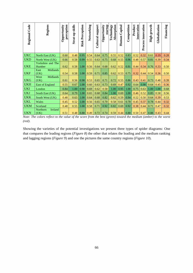
66
Reg
ion
al
Co
de
Reg
ion
s
Op
po
rtu
nit
y
per
cep
tio
n
Str
at-
up
sk
ills
Ris
k P
erce
pti
on
Net
wo
rkin
g
Cu
ltu
ral
sup
po
rt
Op
po
rtu
nit
y
sta
rtu
p
Tec
hn
olo
gy
Ab
sorp
tio
n
Hu
ma
n C
ap
ita
l
Co
mp
etit
ion
Pro
du
ct
inn
ov
ati
on
Pro
cess
in
no
va
tio
n
Hig
h g
row
th
Glo
ba
liza
tio
n
Fin
an
cin
g
UKC North East (UK) 0.60 0.48 0.95 0.54 0.64 0.75 0.55 0.52 0.83 0.52 0.32 0.61 0.19 0.28
UKD North West (UK) 0.66 0.58 0.99 0.55 0.63 0.75 0.68 0.55 0.96 0.48 0.57 0.81 0.39 0.34
UKE Yorkshire and The
Humber 0.62 0.58 1.00 0.56 0.64 0.68 0.62 0.52 0.91 0.44 0.34 0.76 0.33 0.50
UKF East Midlands
(UK) 0.54 0.58 1.00 0.59 0.71 0.85 0.62 0.53 0.75 0.32 0.44 0.54 0.36 0.50
UKG West Midlands
(UK) 0.61 0.56 0.98 0.53 0.65 0.71 0.72 0.55 0.86 0.43 0.41 0.73 0.48 0.39
UKH East of England 0.55 0.67 1.00 0.60 0.63 0.73 0.69 0.47 0.92 0.64 0.98 0.64 0.45 0.36
UKI London 0.84 1.00 0.98 0.69 0.62 0.58 1.00 0.95 1.00 0.75 0.63 1.00 1.00 0.68
UKJ South East (UK) 0.64 0.79 1.00 0.65 0.68 0.84 1.00 0.69 1.00 0.46 0.52 0.85 0.58 0.56
UKK South West (UK) 0.48 0.63 1.00 0.64 0.68 0.82 0.62 0.59 0.94 0.52 0.50 0.64 0.39 0.53
UKL Wales 0.45 0.52 1.00 0.56 0.65 0.70 0.58 0.61 0.78 0.45 0.37 0.78 0.44 0.32
UKM Scotland 0.48 0.55 1.00 0.58 0.71 0.92 0.82 0.69 0.92 0.38 0.44 0.71 0.47 0.32
UKN Northern Ireland
(UK) 0.51 0.48 0.88 0.49 0.72 0.74 0.59 0.44 0.88 0.50 0.47 0.88 0.43 0.44
Note: The colors reflect to the value of the score from the best (green) toward the medium (amber) to the worst
(red).
Showing the varieties of the potential investigations we present three types of spider diagrams: One
that compares the leading regions (Figure 8) the other that relates the leading and the medium ranking
and lagging regions (Figure 9) and one the pictures the same country regions (Figure 10).

67
Figure 8. The comparison of the entrepreneurial profile of the three leading regions
According to Figure 8, all the three leading regions are above the average pillar values in all cases.
Only Hovedstaden’s Globalization is equal to the 125 regions average value of this pillar. All three
regions have some common features: All seems to be strong in Technology Absorption, Human
Capital, Competition and High growth. However, differences are more notable. Hovedstaden is
stronger than the other two regions in Opportunity Perception, Networking, Cultural Support, and
Opportunity Startup, but weak in Risk Perception and Globalization. London’s advantages are the
Startup Skills, Risk Perception, and Globalization pillars. At the same time, London is weak in
Cultural Support, Opportunity Startup, Product Innovation and process Innovation. Íle de France is
strong in Financing, and, similar to London, weak in Cultural Support and Opportunity Startup.
0 0,1 0,2 0,3 0,4 0,5 0,6 0,7 0,8 0,9
1
1. Opportunity
Perception
2. Startup Skills
3. Risk Perception
4. Networking
5. Cultural Support
6. Opportunity Startup
7. Technology
Absorption
8. Human Capital
9. Competition
10. Product Innovation
11. Process Innovation
12. High Growth
13. Globalization
14. Financing
Regional Average Hovedstaden London Île de France

68
Figure 9. The comparison of the entrepreneurial profile of a leading (Stockholm) a medium
ranking (Communidad del Madrid) and a lagging (Közép-Magyarország) region
There are even more differences amongst the three regions in Figure 9. Stockholm is above the
average in all but two pillars, Communidad del Madrid is around the average and Közép-
Magyarország with Budapest is below the average in most pillars. All regions have some strengths and
weaknesses. Stockholm is strong in the Attitudes and Abilities related pillars but weak in Process
Innovation and High Growth. Madrid’s strongest points are Human Capital Product Innovation and
Process Innovation but it is below average in Risk Perception, Opportunity Startup, High Growth and
Globalization. Közép-Magyarország’s Stratup Skills is the pillar with highest value while other pillars
of attitudes, Risk Perception, Networking and Cultural Support are extremely low. By surprise, High
Growth is the highest in Közép-Magyarország amongst the three regions, while Globalization,
Financing and the two innovation related pillars are also critically low.
0 0,1 0,2 0,3 0,4 0,5 0,6 0,7 0,8 0,9
1
1. Opportunity
Perception
2. Startup Skills
3. Risk Perception
4. Networking
5. Cultural Support
6. Opportunity Startup
7. Technology
Absorption
8. Human Capital
9. Competition
10. Product Innovation
11. Process Innovation
12. High Growth
13. Globalization
14. Financing
Regional Average Stockholm
Comunidad de Madrid Közép-Magyarország
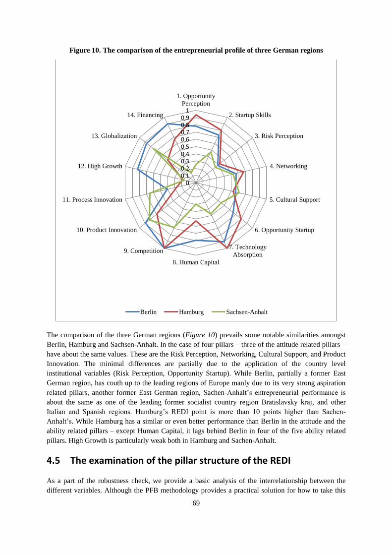
69
Figure 10. The comparison of the entrepreneurial profile of three German regions
The comparison of the three German regions (Figure 10) prevails some notable similarities amongst
Berlin, Hamburg and Sachsen-Anhalt. In the case of four pillars – three of the attitude related pillars –
have about the same values. These are the Risk Perception, Networking, Cultural Support, and Product
Innovation. The minimal differences are partially due to the application of the country level
institutional variables (Risk Perception, Opportunity Startup). While Berlin, partially a former East
German region, has couth up to the leading regions of Europe manly due to its very strong aspiration
related pillars, another former East German region, Sachen-Anhalt’s entrepreneurial performance is
about the same as one of the leading former socialist country region Bratislavsky kraj, and other
Italian and Spanish regions. Hamburg’s REDI point is more than 10 points higher than Sachen-
Anhalt’s. While Hamburg has a similar or even better performance than Berlin in the attitude and the
ability related pillars – except Human Capital, it lags behind Berlin in four of the five ability related
pillars. High Growth is particularly weak both in Hamburg and Sachen-Anhalt.
4.5 The examination of the pillar structure of the REDI
As a part of the robustness check, we provide a basic analysis of the interrelationship between the
different variables. Although the PFB methodology provides a practical solution for how to take this
0 0,1 0,2 0,3 0,4 0,5 0,6 0,7 0,8 0,9
1
1. Opportunity
Perception
2. Startup Skills
3. Risk Perception
4. Networking
5. Cultural Support
6. Opportunity Startup
7. Technology
Absorption
8. Human Capital
9. Competition
10. Product Innovation
11. Process Innovation
12. High Growth
13. Globalization
14. Financing
Berlin Hamburg Sachsen-Anhalt

70
interrelationship into account, it does not save us from examining the underlying structure of the pillar.
It is particularly important to have a well-defined nested structure of whole index.
The arbitrary selection of the pillars would cause confusion, false interpretation, and, finally, a
misleading policy interpretation. The OECD handbook of composite indicators suggests analyzing the
dataset in two dimensions, pillars and observation units, in our case regions (Giovannini et al., 2008).
We have already provided detailed analyses at the regional level; here we are presenting a pillar-level
analysis by calculating the common (Pearson) correlation coefficients. We report correlations between
the original pillars, shown in Table 8, and the correlations between the normalized indicators after
applying the PFB methodology, shown in Table 9.
In general, significant and low to high correlations exist between the pillars in both cases. Most
importantly all the pillars are positively correlate to one another with two exceptions: The correlations
between Process Innovation and Cultural Support and Process Innovation and Human Capital is -0,01
and -0,02, respectively, are insignificant. The pillars Process Innovation and Globalization show the
lowest correlation with the other pillars. However, the PFB, as can be expected, improved the
correlation, implying a closer relationship between the entrepreneurial features. The two, previously
negative insignificantly correlated, pillars have also become positive but weakly correlated pillars. The
positive connection between the entrepreneurship pillars is vital for proper policy interpretation and
suggestions. If the connection between the pillars were negative, it would have implied that one pillar
can only be improved at the cost of the other pillar. In this case, the improvement of the weakest pillar
value would not necessary improve the REDI value.
There are other ways to check out the consistency of the dataset and the potentially strong connection
between the pillars. Both the Kaiser-Meyer-Olkin measure of sampling adequacy and Bartlett’s test of
sphericity reinforce the fact that the 14 pillars of REDI are closely correlated, and it is worth looking
for a single complex measure.8 The most popular test of the internal consistency of the pillars is based
on the Cronbach Coefficient Alpha (c-alpha). The c-alpha value for the 14 pillars is 0.91 with the
original data, and 0.96 after applying the PFB methodology; both are well above the critical 0.7
threshold value. In sum, all of these tests support the internal consistency of the structure as described
with the 14 selected pillars.
8 The Kaiser – Meyer – Olkin measures for the original pillar values are 0.83 and 0.88 for the PFB adjusted
pillars, well above the critical value of 0.50. The Bartlett test is significant at the 0.000 level, excluding the
possibility that the pillars are not interrelated.

71
Table 8. The correlation matrix between the average adjusted pillar values
Average adjusted pillars 1 2 3 4 5 6 7 8 9 10 11 12 13 14 15
1 REDI points 1.00 0.74 0.69 0.60 0.80 0.78 0.80 0.84 0.69 0.84 0.68 0.39 0.48 0.32 0.57
2 Opportunity perception
1.00 0.66 0.44 0.80 0.58 0.67 0.55 0.58 0.51 0.55 0.20 0.35 0.16 0.45
3 Startup skills
1.00 0.24 0.67 0.47 0.53 0.62 0.47 0.51 0.55 0.14 0.34 0.27 0.40
4 Risk perception
1.00 0.40 0.42 0.47 0.43 0.37 0.61 0.18 0.27 0.32 0.11 0.14
5 Networking
1.00 0.81 0.84 0.61 0.55 0.57 0.60 0.15 0.24 0.12 0.53
6 Cultural support
1.00 0.87 0.61 0.61 0.65 0.50 0.14 0.12 -0.01 0.34
7 Opportunity startup
1.00 0.67 0.58 0.68 0.40 0.15 0.15 0.03 0.39
8 Technology adoption
1.00 0.63 0.77 0.56 0.28 0.33 0.19 0.46
9 Human capital
1.00 0.47 0.48 0.25 0.22 -0.02 0.29
10 Competition
1.00 0.50 0.23 0.43 0.31 0.42
11 Product innovation
1.00 0.36 0.33 0.24 0.48
12 Process innovation
1.00 0.19 0.17 0.14
13 High growth
1.00 0.45 0.18
14 Globalization
1.00 0.39
15 Financing
1.00
Bold: Correlation is significant at the 0.01 level (2-tailed).
Italic: Correlation is significant at the 0.05 level (2-tailed).

72
Table 9. The correlation matrix between the pillar values after applying the PFB method
Penalized pillars 1 2 3 4 5 6 7 8 9 10 11 12 13 14 15
1 REDI points 1.00 0.83 0.79 0.70 0.88 0.83 0.85 0.88 0.78 0.89 0.77 0.54 0.62 0.49 0.70
2 Opportunity perception
1,00 0.73 0.57 0.82 0.66 0.70 0.64 0.68 0.64 0.65 0.36 0.51 0.33 0.58
3 Startup skills
1.00 0.42 0.75 0.59 0.63 0.70 0.60 0.64 0.64 0.32 0.49 0.43 0.53
4 Risk perception
1.00 0.54 0.57 0.58 0.56 0.52 0.70 0.36 0.43 0.47 0.28 0.34
5 Networking
1.00 0.85 0.86 0.71 0.64 0.70 0.70 0.34 0.42 0.31 0.65
6 Cultural support
1.00 0.90 0.71 0.69 0.74 0.61 0.34 0.32 0.18 0.50
7 Opportunity startup
1.00 0.75 0.67 0.76 0.53 0.33 0.34 0.22 0.53
8 Technology adoption
1.00 0.72 0.84 0.67 0.45 0.49 0.36 0.59
9 Human capital
1.00 0.60 0.58 0.42 0.39 0.16 0.45
10 Competition
1.00 0.62 0.42 0.58 0.47 0.57
11 Product innovation
1.00 0.50 0.45 0.35 0.61
12 Process innovation
1.00 0.35 0.29 0.33
13 High growth
1.00 0.54 0.34
14 Globalization
1.00 0.51
15 Financing
1.00
Bold: Correlation is significant at the 0.01 level (2-tailed).
Italic: Correlation is significant at the 0.05 level (2-tailed).
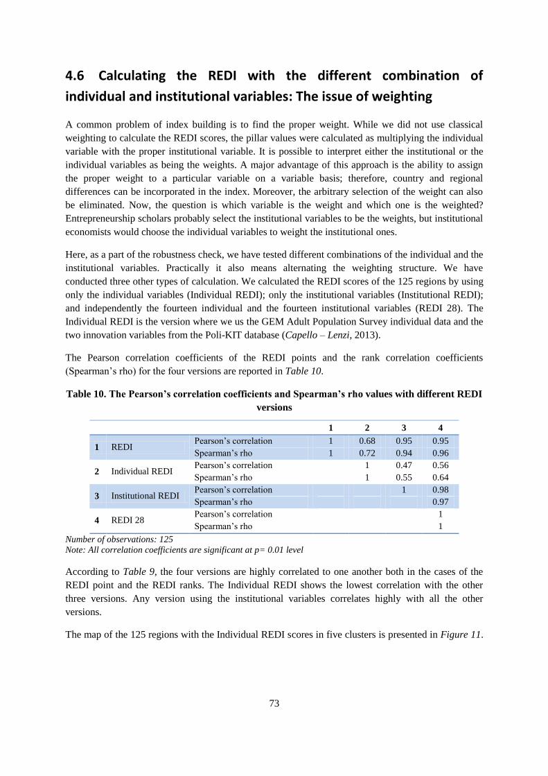
73
4.6 Calculating the REDI with the different combination of
individual and institutional variables: The issue of weighting
A common problem of index building is to find the proper weight. While we did not use classical
weighting to calculate the REDI scores, the pillar values were calculated as multiplying the individual
variable with the proper institutional variable. It is possible to interpret either the institutional or the
individual variables as being the weights. A major advantage of this approach is the ability to assign
the proper weight to a particular variable on a variable basis; therefore, country and regional
differences can be incorporated in the index. Moreover, the arbitrary selection of the weight can also
be eliminated. Now, the question is which variable is the weight and which one is the weighted?
Entrepreneurship scholars probably select the institutional variables to be the weights, but institutional
economists would choose the individual variables to weight the institutional ones.
Here, as a part of the robustness check, we have tested different combinations of the individual and the
institutional variables. Practically it also means alternating the weighting structure. We have
conducted three other types of calculation. We calculated the REDI scores of the 125 regions by using
only the individual variables (Individual REDI); only the institutional variables (Institutional REDI);
and independently the fourteen individual and the fourteen institutional variables (REDI 28). The
Individual REDI is the version where we us the GEM Adult Population Survey individual data and the
two innovation variables from the Poli-KIT database (Capello – Lenzi, 2013).
The Pearson correlation coefficients of the REDI points and the rank correlation coefficients
(Spearman’s rho) for the four versions are reported in Table 10.
Table 10. The Pearson’s correlation coefficients and Spearman’s rho values with different REDI
versions
1 2 3 4
1 REDI Pearson’s correlation 1 0.68 0.95 0.95
Spearman’s rho 1 0.72 0.94 0.96
2 Individual REDI Pearson’s correlation 1 0.47 0.56
Spearman’s rho 1 0.55 0.64
3 Institutional REDI Pearson’s correlation 1 0.98
Spearman’s rho 0.97
4 REDI 28 Pearson’s correlation 1
Spearman’s rho 1
Number of observations: 125
Note: All correlation coefficients are significant at p= 0.01 level
According to Table 9, the four versions are highly correlated to one another both in the cases of the
REDI point and the REDI ranks. The Individual REDI shows the lowest correlation with the other
three versions. Any version using the institutional variables correlates highly with all the other
versions.
The map of the 125 regions with the Individual REDI scores in five clusters is presented in Figure 11.

74
Figure 11. The map of the GEM Individual REDI scores in five categories in 125 European
Union regions, 2013

75
If we compare the original and individual REDI scores we can see that the individual scores have
significantly smaller range and interquartile range than in the original case (Table 11). The
interquartile range is only 8 points and it means that mid 50% of the points are within this range.
Table 11. The descriptive statistics of the original REDI and the Individual REDI scores
REDI scores Individual REDI scores
Average 46.03 63.42
Median 48.21 63.20
Minimum 18.42 46.37
Maximum 82.16 81.04
Range 63.74 34.67
Interquartile range 25.51 8.04
We can see that the Individual REDI score average value (63.42) is much higher than that of the
original REDI scores. Taking into account the lower interquartile range it means that the individual
variables prevail lower differences. Comparing the REDI ranking with the Individual REDI ranking
the changes are substantial, range from +71 to -53. It means, that calculating only with the individual
variables, Jadranska Hrvatska has stepped ahead from the 98th place to the 27
th while the German
Bremen has fallen from the 62nd
to the 115th place. As it can be seen in Figure 11, the scores disperse
in a relatively narrow range. The goodness of fit between the individual REDI scores and the GDP per
capita is weak (R2=0.23), so the individual REDI scores can hardly explain the regional dispersion of
the GDP per capita.
Figure 11 pictures the comparison of the original REDI and the Individual REDI scores and ranking.
The point differences are shown by the blue points and data points are on the primary (left) Y axis
(“Differences in REDI scores with individual variables”). The red points and the secondary (right) Y
axis show us the differences between the original and individual REDI rankings. All of these
“difference figures” show the score differences values in descending order and we can also notice the
ranking differences. It is straightforward from Figure 12 that score changes are in much smaller in
magnitude than the rank changes.

76
Figure 12. The differences in the REDI scores and ranking using the individual variables
The same type of analysis for the Institutional REDI and the REDI 28 has also be done. In both cases
the differences between the original REDI and these two cases are much lower than the case of the
Individual REDI. For the detailed comparison and the new rankings and scores for all the four
versions see Appendix I.
4.7 Robustness analysis: The effect of discarding a pillar
The aim of the robustness analysis is to examine the extent to which the final ranking depends on the
set of choices made during the selection and transformation of the variables included in the sub-
indices. The pillar variables are generally selected according to integrating experts’ judgment, data
availability and checks on statistical consistency. So it is the situation with the REDI, as it has been
described in details in the earlier chapters of this paper. A typical robustness test is to drop out one
pillar at a time and view the changes in the rank of the regions. It is an appropriate method to evaluate
the balance among the pillars in the REDI. This is usually called an uncertainty analysis. We have
calculated the REDI score values with the help of the penalty adjusted method, but we discarded one
pillar at a time. So basically the model just slightly changed. We run fourteen simulations to see the
effect of excluding each pillar one at the time.
The box-plot figure (Figure 13) displays the minimum, maximum values together with the lower and
upper quartile (Q1, Q3) values (range and interquartile range) of the distribution of the difference
between the modified rank, obtained discarding one pillar, and the reference rank, computed on the
basis of the original REDI scores.
-60
-50
-40
-30
-20
-10
0
10
20
30
40
50
60
70
80
-10
-5
0
5
10
15
20
25
30
35
40
45
Dif
feren
ces
bet
wee
n o
rig
ina
l a
nd
ind
ivid
ua
l R
ED
I ra
nk
ing
Dif
feren
ces
in R
ED
I sc
ore
s u
sin
g t
he
ind
ivid
ua
l v
ari
ab
les
Score diff.
Rank diff.

77
Figure 13. Distribution of the rank differences
(uncertainty analysis discarding one pillar at a time)
All the interquartile ranges are between the band -2 and +2, meaning that, for all the simulations, in
50% of the cases the maximum shift of the region rank is up to only 2 positions wide. This indicates a
very balanced role of the pillars. The total ranges (maximum-minimum) are between -11 and +11 in
case of 11 indicators. The three most influencing variables are the Process innovation, High growth
and Cultural support. The highest differences are due to the extremely weak performance of these
three pillars in three regions. Cultural support is 0.06 in Bratislavsky kraj (Slovakia), Process
innovation is 0.07 only in Brandenburg (Germany), and High growth is 0.09 in Bremen (Germany).
Excluding these extreme value pillars the three regions stepped ahead a lot in the ranking. Beyond
these three extreme cases the minimum and maximum differences are within +18 and -11. If we take
into account that altogether 125 regions are in the analysis, these shifts clearly show the balanced
construction of the pillars and the overall REDI.
Looking at the Spearman rank correlation coefficients in Table 12 we feel that the earlier statement is
even more confirmed. In each case of the simulations the new ranks are in a very strong stochastic
relationship (values are above 0.99) with the original ranking.
-10
-5
0
5
10
15
20
25
30
35
40
Max
Q3
Q1
Min
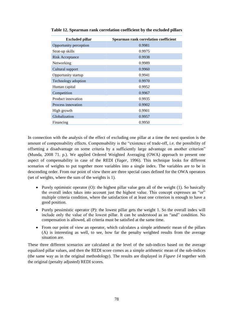
78
Table 12. Spearman rank correlation coefficient by the excluded pillars
Excluded pillar Spearman rank correlation coefficient
Opportunity perception 0.9981
Strat-up skills 0.9975
Risk Acceptance 0.9938
Networking 0.9989
Cultural support 0.9960
Opportunity startup 0.9941
Technology adoption 0.9970
Human capital 0.9952
Competition 0.9967
Product innovation 0.9935
Process innovation 0.9902
High growth 0.9901
Globalization 0.9957
Financing 0.9950
In connection with the analysis of the effect of excluding one pillar at a time the next question is the
amount of compensability effects. Compensability is the “existence of trade-off, i.e. the possibility of
offsetting a disadvantage on some criteria by a sufficiently large advantage on another criterion”
(Munda, 2008 71. p.). We applied Ordered Weighted Averaging (OWA) approach to present one
aspect of compensability in case of the REDI (Yager, 1996). This technique looks for different
scenarios of weights to put together more variables into a single index. The variables are to be in
descending order. From our point of view there are three special cases defined for the OWA operators
(set of weights, where the sum of the weights is 1).
Purely optimistic operator (O): the highest pillar value gets all of the weight (1). So basically
the overall index takes into account just the highest value. This concept expresses an “or”
multiple criteria condition, where the satisfaction of at least one criterion is enough to have a
good position.
Purely pessimistic operator (P): the lowest pillar gets the weight 1. So the overall index will
include only the value of the lowest pillar. It can be understood as an “and” condition. No
compensation is allowed, all criteria must be satisfied at the same time.
From our point of view an operator, which calculates a simple arithmetic mean of the pillars
(A) is interesting as well, to see, how far the penalty weighted results from the average
situation are.
These three different scenarios are calculated at the level of the sub-indices based on the average
equalized pillar values, and then the REDI score comes as a simple arithmetic mean of the sub-indices
(the same way as in the original methodology). The results are displayed in Figure 14 together with
the original (penalty adjusted) REDI scores.

79
Figure 14. REDI scores calculated with different scenarios of the OWA operators
As an obvious result, the average and the original REDI scores move between the pessimistic and the
optimistic lines. It is also clear, that the aim of the penalty adjusted was reached, as the original REDI
scores are always below the average line. It means that compensability is restricted within the REDI
indicator, and a balanced performance is rewarded. It is also important to look at the result at the level
of the regions. What is the variability of the different scenarios within the regions? Regions with very
low pessimistic REDI scores are also those with very high optimistic results.
Detailed data of the 17 most effected regions can be found in Table 13. Beside the average equalized
data of the pillars the table includes the original REDI score and ranks, the scores based on the three
scenarios (REDI(O) – optimistic, REDI(P) – pessimistic, REDI(A) – average), and the difference
between the optimistic and pessimistic scores.) They are those regions that are influenced by the
compensability effect the most. In addition, they are the most sensitive ones with respect to the change
of the weighting scheme. It means those regions where the average distance (range) of the lowest and
highest pillars within the sub-indices is the highest. In Table 13 the orange cells indicate the highest
values within the sub-index, and the green ones the lowest values. It does not necessarily mean to have
very high and very low values at the same time; however at one end (minimum or maximum) the
values are “extreme” within the sub-indices. These 17 regions are coming randomly from every part of
the original REDI ranking (the ranks can be seen in the grey row of Table 13), which means, that the
sensitivity to compensability is independent from the overall position of the regions.
0
10
20
30
40
50
60
70
80
90
100 D
K0
1
DK
05
DK
02
SE
22
FI1
B
DE
7
AT
1
UK
K
FR
6
NL
2
UK
E
DE
2
ES
30
FR
2
UK
C
AT
3
DE
F
SI0
1
PL
1
CZ
ES
53
ES
11
ES
41
PL
4
HU
10
HR
04
ES
43
PT
16
RO
3
EL
4
HU
32
HU
33
REDI REDI (O) REDI (P) REDI (A)

80
Table 13. The 17 most effected regions by the changes of the weight
GEO code NL1 DE4 DE5 BE1 DK03 FR2 RO4 HU10 SE32 DK04 RO3 DK02 FI19 NL3 AT1 UKH DK05
GEO title
No
ord
-Ned
erl
an
d
Bra
nd
en
bu
rg
Brem
en
Rég
ion
de B
ru
xell
es-
Ca
pit
ale
Sy
dd
an
mark
Ba
ssin
Pa
risi
en
Ma
croreg
iun
ea p
atr
u
Kö
zép
-Mag
ya
rorsz
ág
Mell
erst
a N
orrl
an
d
Mid
tjy
lla
nd
Ma
croreg
iun
ea t
rei
Sja
lla
nd
Lä
nsi
-Su
om
i
West
-Ned
erl
an
d
Ost
öst
err
eich
Ea
st o
f E
ngla
nd
No
rd
jyll
an
d
Opportunity perception 0.39 0.33 0.56 0.76 0.95 0.36 0.31 0.54 0.99 1.00 0.43 0.90 1.00 0.88 0.77 0.55 0.91
Strat-up skills 0.71 0.73 0.57 0.86 0.45 0.29 0.03 0.79 0.64 0.46 0.04 0.48 1.00 1.00 0.86 0.67 0.40
Risk Acceptance 0.29 0.37 0.39 0.90 0.64 0.78 0.79 0.15 0.72 0.62 0.77 0.64 0.60 0.29 0.40 1.00 0.61
Networking 0.80 0.51 0.74 0.50 0.90 0.49 0.07 0.29 1.00 1.00 0.09 0.96 0.97 0.88 0.65 0.60 1.00
Cultural support 1.00 0.55 0.58 0.37 1.00 0.57 0.08 0.07 0.71 1.00 0.03 1.00 0.70 1.00 0.48 0.63 1.00
Opportunity startup 0.96 0.54 0.50 0.34 1.00 0.58 0.02 0.14 1.00 1.00 0.01 0.95 0.92 0.79 0.63 0.73 1.00
Technology adoption 0.45 0.69 0.53 1.00 0.51 0.76 0.17 0.52 0.66 0.68 0.19 0.62 0.80 0.76 0.72 0.69 0.70
Human capital 0.30 0.77 0.99 1.00 1.00 0.24 0.24 0.54 0.64 1.00 0.36 0.98 0.84 0.55 0.40 0.47 1.00
Competition 0.52 1.00 0.65 0.58 0.85 0.83 0.17 0.28 0.63 0.83 0.18 0.69 0.36 0.90 0.84 0.92 0.80
Product innovation 0.78 0.61 1.00 0.97 1.00 0.55 0.03 0.22 0.26 1.00 0.09 0.88 0.79 0.83 0.78 0.64 0.92
Process innovation 0.28 0.07 0.37 0.50 0.35 0.91 0.30 0.26 0.17 0.28 0.55 0.88 0.81 0.42 0.53 0.98 0.76
High growth 0.42 1.00 0.09 1.00 0.55 0.35 0.65 0.71 0.07 0.76 0.57 0.81 0.57 0.67 0.37 0.64 0.76
Globalization 0.48 0.97 0.97 0.97 0.42 0.64 0.49 0.29 0.51 0.31 0.48 0.19 0.22 0.65 0.79 0.45 0.40
Financing 0.61 0.64 0.66 0.60 0.62 0.62 0.09 0.38 0.94 0.64 0.13 0.52 0.30 0.89 1.00 0.36 1.00
REDI 51.1 48.5 48.4 64.9 65.1 50.9 19.7 31.4 48.2 64.3 22.1 60.7 58.7 64.4 60.7 61.5 72.0
REDI rank 53 61 62 13 12 54 122 99 63 16 116 23 32 15 25 22 8
REDI (O) 91.2 91.0 91.2 96.8 100.0 84.1 56.2 68.1 97.9 100.0 56.6 95.4 91.2 93.1 90.1 96.9 100.0
REDI (P) 29.0 31.6 32.9 40.3 43.5 29.5 2.5 14.5 44.7 47.2 4.4 43.4 39.4 41.8 39.1 46.1 49.9
REDI (A) 57.0 63.5 61.8 73.9 73.7 57.2 23.9 37.1 64.5 76.4 27.3 75.6 70.8 75.1 65.8 67.0 80.9
REDI(O)-REDI(P) 62.3 59.4 58.3 56.5 56.5 54.6 53.7 53.6 53.2 52.8 52.1 52.1 51.8 51.3 51.1 50.8 50.1
Uncertainty analysis together with the compensability effect analysis supports the robustness of the
REDI indicator. The results justify, that the index provides a synthetic picture of the regional
entrepreneurship within the European Union at the level of regions, while representing a balanced
diversity of the different aspects (pillars).
We have also conducted other robustness checks examining the consequences of changing the
variables. In all cases the changes of the scores and ranking was minimal. Out of these checks we
show the effects of changing two institutional variables on the REDI scores and the ranking Appendix
J.
4.8 The comparison of REDI to other regional indices
In this part of the report we compare the REDI scores and rankings to other available regional level
indexes:

81
Regional Competitiveness Index (RCI)
Regional Innovation Scoreboard (RIS)
Quality of Government Index (QoG)
Regional Corruption Index
Note that three out of the four indices were used partially or fully in the REDI as measuring various
institutional dimensions of regional level entrepreneurship. Therefore it can be expected that these
indices should show a significant correlation and close relationship to REDI.
The EU Regional Competitiveness Index (RCI 2013) intended to measure and to examine the various
levels of competitiveness at the regional level. “RCI 2013 reveals a strong regional dimension of
competitiveness, which national level indicators cannot capture. The RCI shows the strengths and
weaknesses of each of the EU NUTS2 regions. It can provide a guide to what each region should focus
on, taking into account its specific situation and its overall level of development.”
(Source:http://ec.europa.eu/regional_policy/information/studies/index_en.cfm#3 2013.09.28.)
The RCI uses only institutional variables to measure regional competitiveness. The RCI contains 3
sub-indexes which build up 11 pillars: (I) Basic Sub-index: (1) Institutions (2) Macroeconomic
Stability (3) Infrastructure (4) Health (5) Basic Education (II) Efficiency Sub-index: (1) Higher
Education and Lifelong Learning (3) Labor Market Efficiency (4) Market Size (III) Innovation Sub-
index: (1) Technological Readiness (2) Business Sophistication (3) Innovation. The index scores have
been calculated for 274 regions of the European Union.
For comparing the RCI with REDI, the missing NUTS1 level data were calculated as the population
weighted average of NUTS2 level RCI data (Austria, Belgium, Germany, France, Greece, Italy, The
Netherlands, Poland, Romania and United Kingdom). In the REDI we applied several parts of the
RCI: three RCI Business Sophistication variables /(1) Employment in J,K sectors, (2) GVA in J,K
sectors and (3) FDI intensity/ were used as part of the REDI Business Strategy institutional variable
(Competition pillar). The data of Employment in J,K variable was updated. Also five RCI Innovation
variables /(1) Total patent application, (2) Scientific publications, (3) High-tech inventors, (4) ICT
inventors, (5) Biotechnology inventors/ were used to create REDI Technology Transfer institutional
variable (Product Innovation pillar). Except Scientific publications variable, all variables were
updated. Furthermore, the three RCI Infrastructure variables /(1) Motorway density, (2) Railway
density, (3) Number of passenger flights/ were used to determine the Connectivity institutional
variable (Internationalization pillar).
The connection between the REDI Index and the EU Regional Competitiveness Index (RCI 2013) is
positive and significant, as expected. Using third degree polynomial trend-line, it explains 76% of the
variance between the two indices (Figure 15).
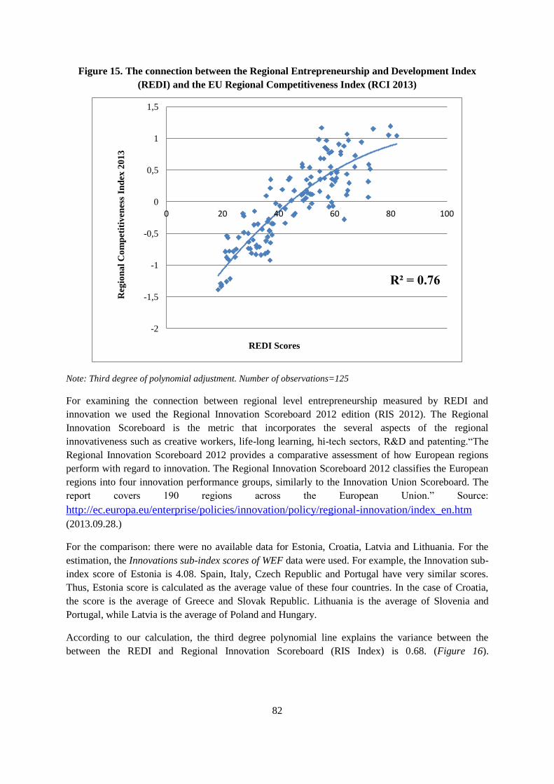
82
Figure 15. The connection between the Regional Entrepreneurship and Development Index
(REDI) and the EU Regional Competitiveness Index (RCI 2013)
Note: Third degree of polynomial adjustment. Number of observations=125
For examining the connection between regional level entrepreneurship measured by REDI and
innovation we used the Regional Innovation Scoreboard 2012 edition (RIS 2012). The Regional
Innovation Scoreboard is the metric that incorporates the several aspects of the regional
innovativeness such as creative workers, life-long learning, hi-tech sectors, R&D and patenting.“The
Regional Innovation Scoreboard 2012 provides a comparative assessment of how European regions
perform with regard to innovation. The Regional Innovation Scoreboard 2012 classifies the European
regions into four innovation performance groups, similarly to the Innovation Union Scoreboard. The
report covers 190 regions across the European Union.” Source:
http://ec.europa.eu/enterprise/policies/innovation/policy/regional-innovation/index_en.htm
(2013.09.28.)
For the comparison: there were no available data for Estonia, Croatia, Latvia and Lithuania. For the
estimation, the Innovations sub-index scores of WEF data were used. For example, the Innovation sub-
index score of Estonia is 4.08. Spain, Italy, Czech Republic and Portugal have very similar scores.
Thus, Estonia score is calculated as the average value of these four countries. In the case of Croatia,
the score is the average of Greece and Slovak Republic. Lithuania is the average of Slovenia and
Portugal, while Latvia is the average of Poland and Hungary.
According to our calculation, the third degree polynomial line explains the variance between the
between the REDI and Regional Innovation Scoreboard (RIS Index) is 0.68. (Figure 16).
R² = 0.76
-2
-1,5
-1
-0,5
0
0,5
1
1,5
0 20 40 60 80 100
Reg
ion
al
Co
mp
etit
iven
ess
Ind
ex 2
01
3
REDI Scores

83
Figure 16. The connection between the Regional Entrepreneurship and Development Index
(REDI) and the Regional Innovation Scoreboard (RIS 2012)
Note: Third degree of polynomial adjustment. Number of observations=125
The European Quality of Government Index (QoG Index) and the Regional Corruption Index are
coming from the same survey. In fact, the Regional Corruption Index is a part of the QUG Index. “The
QoG EU Regional Data is the result of a survey of corruption on a regional level within the EU
conducted during 2010. It covers all 27 member states and a 172 NUTS 1 and NUTS 2 regions. In
total the survey was answered by 34 000 respondents creating the most complete quantitative estimate
of QoG to date. The national level estimates are taken from the World Bank Governance Indicators.
The regional estimates are comprised of 16 separate indicators.” (Source:
http://www.qog.pol.gu.se/data/datadownloads/qogeuregionaldata/ 2013.09.28.)
The QoG Index was re-scaled (converted to a scale of 0 to 10). In the case of REDI, the QoG index
was employed to measure REDI Business Environment institutional variable (Opportunity Startup
pillar), and Regional Corruption Index was used in order to determine REDI Personal Freedom
institutional variable (Cultural Support pillar). The Regional Corruption Index is the only institutional
variable that appears two times in the REDI, first as a part of the QoG Index and second as an
independent regional institutional variable in the Cultural Support.
The third degree polynomial line explains 61 percent of the variation in the case of the QoG (Figure
17) and 68 percent in the case of the Regional Corruption Index (Figure 18).
R² = 0.68
0
0,1
0,2
0,3
0,4
0,5
0,6
0,7
0,8
0 10 20 30 40 50 60 70 80 90
Reg
ion
al
Inn
ov
ati
on
Sco
reb
oa
rd
REDI Scores

84
Figure 17. The connection between the Regional Entrepreneurship and Development Index
(REDI) and the Quality of Governance Index (QoG Index)
Note: Third degree polynomial trend-line
Figure 18. The connection between the Regional Entrepreneurship and Development Index
(REDI) and the Regional Corruption Index
Note: Third degree polynomial trend-line
R² = 0.61
0
2
4
6
8
10
12
0 10 20 30 40 50 60 70 80 90
Qo
G (
resc
ale
d)
REDI Scores
R² = 0.68
0
2
4
6
8
10
12
0 20 40 60 80 100
Reg
ion
al
Co
rru
pti
on
REDI Scores

85
Furthermore, as we can see from the correlation table (Table 14) that all the four indices correlate
significantly with the Regional Entrepreneurship and Development Index. Moreover, all five regional
indices have a strong connection with the per capita GDP. This finding is not a surprise since all of
them aim to explain different dimensions of regional development.
Table 14. Correlations coefficients between REDI GDP per capita and four regional indices
1 2 3 4 5 6
1 REDI 1 0.70 0.82 0.86 0.75 0.77
2 GDP per capita
1 0.72 0.74 0.48 0.47
3 Regional Innovation Scoreboard
1 0.85 0.68 0.63
4 Regional Competitiveness Index
1 0.72 0.69
5 Quality of Government
1 0.85
6 Regional Corruption Index
1
Note: All correlations are significant at the 0.01 level

86
5 Policy Application of the REDI Methodology
5.1 Entrepreneurship Policy in the European Union
The shift from a ‘managed’ economy to an ‘entrepreneurial’ economy is among the most important
challenges developed economies have faced over the last few decades. This challenge is closely
coupled with the increasing importance of non-physical capital, such as human and intellectual capital
for wealth creation. The most notable signs of this shift are the following: (1) knowledge is
increasingly replacing physical capital and labor as the key driving force of economic growth; (2)
individuals rather than large firms are the leading factor in new knowledge creation; (3) alongside with
large conglomerates, new and small firms play a dominant role in translating newly created knowledge
into marketable goods and services; (4) traditional industrial policy, with antitrust laws and small
business protection, has been replaced by a much broader entrepreneurship policy aiming to promote
entrepreneurial innovation and facilitate high-growth potential start-ups (Audretsch, 2007; Audretsch –
Thurik, 2001; Henrekson – Stenkula, 2009; Autio et al., 2007).
This re-location of emphasis from ‘dinosaurs to mice’ first begun in the United States, as it took the
lead in the transformation from managed to an entrepreneurial economy (Acs, Carlsson and Karlsson,
1999; Grilo – Thurik, 2005; Freytag –Thurik, 2007). In Europe, this transformation begun a little later,
but by 2000, the European Union had fully recognized the importance of entrepreneurship in
promoting economic dynamism. In the 2000 Lisboa Strategy former European Commission president
Romano Prodi confirmed that “…there is mounting evidence that the key to economic growth and
productivity improvements lies in the entrepreneurial capacity of an economy” (cited by Audretsch,
2009: 256). In 2003, the Green Paper on entrepreneurship provided further detail to the Member States
on how to strengthen entrepreneurship (Green Paper, 2003).
With an improved understanding of the economic contributions of entrepreneurship, also policy
emphasis has gradually evolved. Initially, much of the policy focus was on ‘small business’, and
entrepreneurship was often interpreted as small business activity. Consistent with this interpretation,
the EU launched several initiatives, from encouraging entrepreneurial attitudes, supporting
entrepreneurial education, culture, and decreasing the administrative and financial burdens to foster
business start-up. The Small Business Act (2008) summarizes the most important tenet of small
business support and entrepreneurship as “Think small first”.
Alongside with an early emphasis on small business, there has been a consistent focus on promoting
innovation and technology transfer through small start-ups. This emphasis has been reflected in policy
initiatives designed to support new business incubators and science parks, notably in the vicinity of
universities and higher education institutions. There have also been initiatives to promote networking
among science parks (both nationally and internationally), as well as promoting investment in R&D
and associated collaboration in new and small firms. This emphasis is also reflected in policy
initiatives targeting ‘Knowledge-Intensive Services’ (KIS).
A major re-orientation in policy thinking was subsequently prompted by the gradual observation that
not all new firms contribute equally to employment creation. Instead, studies have shown that only a
small minority of new firms in any given cohort will end up creating the bulk of the economic impact
created by any new firm cohort (Autio, 2006). This observation has prompted a number of initiatives
to elaborate the implications of this observation for policy design, including the ‘Gazelles’ expert
87
work group under the EU Innova Program (Autio – Hoeltzl, 2008). Among the most visible
manifestations of this thinking are encapsulated in the EU Knowledge Intensive Services program and
the evolving new venture accelerator initiatives.
Summarizing, three distinct foci can be identified in EU entrepreneurship policy, as it has evolved
over time: (1) focus on SMEs; (2) focus on innovation through SMEs; and (3) focus on high-growth
SMEs. These co-existing foci reflect evolution in the understanding of the varied roles that
entrepreneurship can play in economic development. However, although each of these focus areas
adds important elements to the European economic policy toolbox, none of them alone provides a
definitive answers to the diverse and varied challenges that different European regions face, as they
seek to implement policies to enhance regional dynamism and competitiveness.
The most recent evolution in entrepreneurship policy – an increasing emphasis on taking a more
holistic and multi-pronged view of entrepreneurship, as advocated by the ‘entrepreneurship support
ecosystem’ thinking – represents yet another evolution in European policy thinking. The focus on
‘entrepreneurship ecosystems’ calls attention to entrepreneurship support policies and initiatives over
the entire lifecycle of the new venture, the key insight being that entrepreneurship support should be
considered in a wider regional context. Thus, this emphasis naturally shifts focus towards a regional
level of analysis, consistent with the focus of this current report and its ‘Systems of Entrepreneurship’
approach. Yet, although similar on the surface, the two concepts are fundamentally different. Whereas
the notion of ‘Entrepreneurship Ecosystems’ focuses on entrepreneurship support policies and
initiatives from a policy perspective, the notion of ‘Systems of Entrepreneurship’ draws attention to
the entrepreneurial dynamic that ultimately drives productivity growth in regions. The two approaches
therefore complement one another, and the REDI index should provide important guidance for the
design of entrepreneurship support ecosystems.
The REDI index should also lend itself for supporting another, perhaps even more important recent
evolution in EU regional and economic policy, notably, the EU Smart Specialization policy. This is a
new and evolving focus that has particular relevance in the context of EU regional and cohesion
policy. In the following, we suggest that the ‘Systems of Entrepreneurship’ approach, as described
earlier in this report, and the systemic REDI index exhibit features that resonate positively with the
Smart Specialization policy emphasis.
5.2 Regional Systems of Entrepreneurship and Smart
Specialization
In this report we have argued that at the regional level, entrepreneurship should be treated as a
systemic phenomenon, and it should be measured accordingly. Although entrepreneurial actions are
ultimately undertaken by individuals, these individuals are always embedded in a given regional
context. This context regulates who becomes an entrepreneur, what the ambition level of the
entrepreneurial effort is, and what the consequences of entrepreneurial actions are. Because of this
embeddedness and the regulating influence of context, we have chosen to develop a complex
composite index that captures both individual-level actions as well as contextual influences. The key
idea of this systemic index is that system performance is “co-produced” by its constituent elements.
This means that the different system components are inter-related. For example, even ambitious
entrepreneurs cannot grow their ventures if they cannot access the necessary resources. Technology-
based new ventures will find it difficult to innovate if the regional job market does not supply

88
workforce with the required specialist skills. In a regional system of entrepreneurship, it is the
combination of the different components that ultimately determines whether the system will function
well or not. The REDI index has been designed to provide a holistic view into the functioning of EU’s
Regional Systems of Entrepreneurship, and we believe that it should be of particular utility when
identifying gaps and bottlenecks that prevent a given region from fully exploiting its entrepreneurial
potential.
National and Regional Research and Innovation Strategies for Smart Specialization represent
European Commission’s answer to the challenge of improving European competitiveness. Set out in
the Innovation Union document published in 2010 (EU Commission, 2010), Smart Specialization
Strategies are policy agendas that build on each country’s and region’s strengths to focus policy
initiatives on key national and regional priorities, challenges and needs for knowledge-based
development (EU Commission, 2012). At the heart of this approach is the identification and leveraging
of each region’s distinctive strengths and unique characteristics that can be harnessed to facilitate
innovation-based regional competitive advantages (Foray et al., 2009). According to EU definition,
“Smart specialization means identifying the unique characteristics and assets of each country and
region, highlighting each region’s competitive advantages, and rallying regional stakeholders and
resources around an excellence-driven vision of their future” (EU Commission, 2012).
The centrality of Smart Specialization Strategies is for EU competitiveness policy is highlighted by the
fact that an explicit Smart Specialization Strategy will be a precondition for using the European
Regional Development Fund (ERDF) funding to support investments in research and innovation in EU
regions (EU Commission, 2012). To receive funding from ERDF and from EU Structural and
Cohesion funds, EU regions need to be able to articulate their strategies for building on their
distinctive regional strengths. This, for its part, makes it necessary for regions to recognize their
strengths – as well as their weaknesses. Identifying these strengths and weaknesses will therefore be a
priority, as EU moves towards implementing the ‘Horizon 2020’ strategy.
However, implementing Smart Specialization strategies is challenging because of the well-known
‘Picking the Winners’ problem: how can policy-makers decide which regional strengths to pick and
invest in, and which ones to abandon? Predicting technological progress is notoriously difficult, and
consequently, it is difficult to predict which regional features will provide the foundation for future
strengths and weaknesses. As an answer to this conundrum, the Smart Specialization concept
advocates the notion of ‘Entrepreneurial Discovery’ (Foray et al., 2009; McCann – Ortega-Argilés,
2013). As defined by the European Commission, the process of Entrepreneurial Discovery is not a top-
down process, but rather, “…involves businesses, research centers and universities working together
to identify a Member State or region’s most promising areas of specialization, but also the weaknesses
that hamper innovation there” (EU Commission, 2012). As noted by Foray et al (2009:2),
“…entrepreneurial actors are likely to play leading roles in discovering promising areas of future
specialization” in exploring needed adaptations to local skills, materials, market access conditions, and
environmental conditions. However, the authors do not elaborate on how this process is supposed to
operate in practice. McCann et al (2013:9) shed a little more light on this question, noting that
entrepreneurs should play a leading role in identifying viable technological diversification
opportunities in regions: “…it is the entrepreneurs and not the regional policy-makers who are
assumed to be best equipped for identifying smart specialization opportunities…”. The implication
here is that regional policy-makers should facilitate conditions in which entrepreneurs can effectively
search and discover opportunities for smart specialization. Regional policy-makers, then, can learn

89
from the discoveries made by entrepreneurs and translate these into Smart Specialization Strategies for
the region.
While the above guidance provides some pointers as to how the Entrepreneurial Discovery process is
assumed to work, it also leaves many questions unanswered: how do entrepreneurs know when they
have discovered new regional strengths? How will policy-makers know this? How exactly are policy-
makers supposed to learn from entrepreneurs, and how are salient lessons going to be encapsulated in
Smart Specialization Strategies for the region? Clearly, while some progress has been made in treating
Smart Specialization challenges at conceptual and theoretical levels, practical guidance is still rather
vague.
We suggest that the distinctive features of the REDI index – notably, its systemic approach and the
Penalty for Bottleneck feature – can be leveraged to support Entrepreneurial Discovery processes in
two distinct ways, as EU regions develop Smart Specialization Strategies. First, the index itself
provides initial clues on whether a given region’s strengths and weaknesses might be found. Second –
and more importantly, the REDI index can be used as a platform that facilitates the design of effective
policies to support Entrepreneurial Discovery. If used in a correct way, therefore, the REDI index can
support the preconditions for creating Smart Specialization Strategies.
As is clear from our discussion of the Systems of Entrepreneurship theory, entrepreneurial dynamics
in regions are complex, and an understanding of them requires a holistic approach. This is why the
REDI index was designed to incorporate 14 different pillars, each created as a product of individual-
level and system-level data. A careful scrutiny of the relative differences between individual pillars,
both within a given region and across benchmark regions, should provide good initial guidance for the
search of prospective strengths and weaknesses within regions. From a policy perspective, it is
important to recognize that the portfolio of policy measures to address regional are likely to be equally
complex and intertwined as is the system itself. Therefore, a complex and multi-dimensional index (as
opposed to a uni-dimensional one) should be mirrored by a systemic approach to policy portfolio
design (as opposed to a siloed approach).
Second, and as a more important aspect, the REDI index should assist regions in creating conditions
for effective Entrepreneurial Discovery – i.e., in creating conditions in which the region’s
entrepreneurial dynamic operates efficiently. Achieving this requires a deep understanding of how the
region’s System of Entrepreneurship works, what the most important bottlenecks are, and how these
could be alleviated. To achieve this understanding, it is important to go beyond the ‘hard’ numbers, as
suggested by the REDI index. Any System of Entrepreneurship will be infinitely more complex than
what an index like the REDI index can capture. Therefore, in order to gain an understanding of how a
given region’s System of Entrepreneurship works, it is important to complement the REDI index with
a stakeholder engagement process that is designed to draw out ‘soft’ insights from various policy
stakeholders on what makes the Regional System of Entrepreneurship really work. A suggested
approach could work as follows:
First, conduct a REDI analysis of the region, creating a preliminary list of regional strengths
and weaknesses, as suggested by the REDI index
Second, invite regional entrepreneurship policy stakeholders into a Stakeholder Engagement
Workshop that debates the REDI analysis

90
Third, draw on the stakeholders’ varied perspectives and insights to enrich the REDI analysis
and complement REDI data with stakeholders’ experience-based insights on the regional
realities and entrepreneurial dynamics
Fourth, collect additional data to further analyze the region’s entrepreneurial strengths and
weaknesses
Fifth, conduct further workshops to identify policy actions that can alleviate regional
bottlenecks and further improve regional strengths
Sixth, design an implementation plan to improve the dynamic of the Regional System of
Entrepreneurship
Used this way, the REDI index should provide a platform that can be leveraged for the design and
facilitation of Smart Specialization Strategies in EU regions.
Finally, the REDI index can be used to identify regional policy priorities through an Entrepreneurship
Policy Portfolio Optimization Exercise. An important implication of the REDI analysis is that
reducing the differences between the pillars is the best way to increase the value of the indicator. In
order to reduce the differences between the pillars the most straightforward way of doing it is by
enhancing the weakest REDI pillar. However, another pillar may become the weakest link
constraining the performance in the overall entrepreneurship activity. This system dynamics leads to
the problem of “optimal” allocation of the additional resources. In other words, if a particular region
were to allocate additional resources to improving its REDI Index performance, how should this
additional effort be allocated to achieve an “optimal”9 outcome?
5.3 Regional entrepreneurship policy: Optimizing the resource
allocation
As a systemic index, the REDI permits the exploration of different policy scenarios. Because of the
Penalty for Bottleneck algorithm, one tempting use of the REDI index is in exploring alternative sce-
narios for enhancing the entrepreneurial performance of the regional System of Entrepreneurship – as
captured by the REDI index. This is because the PFB algorithm ‘penalises’ system pillars according to
gaps exhibited by the most poorly performing pillar – i.e., the ‘Bottleneck’ pillar. As explained above,
the idea is that systems with strong weaknesses cannot fully leverage their strengths: to put another
way, weakly performing Bottleneck pillars hold back system performance in situations where system
pillars co-produce system performance. A corollary implication of this assumption is that policy effort
is allocated most effectively when it seeks to alleviate systemic bottlenecks. Instead of further
enhancing systemic strengths, it may be more effective to alleviate the bottlenecks that prevent the
system from fully leveraging its strengths.
Using the logic above, we performed a series of simulations exploring the effect of policies designed
to alleviate systemic bottlenecks. We have conducted the simulation for all 125 regions but analyze the
outcomes only briefly for regional policy implications. The simulation seeks to identify the ‘most
efficient’ allocation of policy effort that seeks to increase the REDI index score by 10 points. The PFB
method calculation implies that the greatest improvement in system performance can be achieved by
alleviating the weakest performing pillar – the Bottleneck Pillar. In the simulation, each Bottleneck
Pillar is alleviated to a point where it seazes to be a bottleneck. At this point, any further effort is
9‘Optimal’ is interpreted in the sense of maximizing the REDI value.

91
allocated to the second-most binding constraint within the system, again up to a point where this
constraint is no longer the most binding constraint within the system. By successively alleviating most
binding constraints, our simulation therefore provides an idea of how policy effort should be allocated
to achieve an ‘optimal’ outcome, defined as the largest possible increase in the REDI index score.
Table 15 shows the result of this optimization exercise for all the 125 regions of the 24 EU countries.
Note that our simulation rests on a number of constraining assumptions. First, the optimization focuses
on the REDI index score, assuming that this score fully reflects the entrepreneurial performance of the
system. As we have already noted, systems of entrepreneurship are inherently more complex than any
index can capture, so this assumption is restrictive. Second, the simulation assumes that all pillars are
equally amenable to manipulation through policy effort. In reality, some pillars can be addressed more
easily than others. Third, we have assumed that the cost of improving the value of any pillar is
constant. Obviously, some pillars can be more costly to change than others. Across regions, the cost of
an improvement of a pillar in larger region like London could also be considerably higher than in a
smaller region like Dél Dunántúl in Hungary. Fourth, the PFB is applied equally to all pillars,
assuming that all system pillars are equally connected. In reality, some pillars may obviously be more
closely connected to one another than to some other pillars. These assumptions mean that the results of
the simulation exercise should not be taken as a final truth or as normative policy prescriptions.
Instead, the purpose of the simulation exercise is simply to illustrate possible system dynamics under
different scenarios. These simulations should then be debated case by case in different regions. Such a
debate, we believe, will serve to extract and illuminate region-specific aspects and specialities, which
then could inform, e.g., the design of Smart Specialisation Strategies in regions.
Even if the assumptions are restrictive and should be kept in mind, the policy portfolio simulation
offers many benefits that go above and beyond what traditional indices can offer. The most important
benefit is in drawing attention and highlighting system dynamics in Regional Systems of
Entrepreneurship. This reinforces a systemic perspective to policy analysis and design over a
traditional, siloed perspective. A policy scenario simulation that highlights interconnections within the
system also forces policy analysts and policy-makers to think outside individual policy silos and
consider the system performance as a whole. This, then, should help policy-makers also to think about
trade-offs between different allocations of policy effort and judge their effectiveness against a system-
level performance benchmark. If correctly used, therefore, a policy portfolio simulation should
facilitate agreement on system-level policy priorities. This kind of simulation should also help
promote awareness of different policy scenarios and associated trade-offs.
The tables below assume a constant amount of additional policy effort, which is distributed across
constraining pillars until a 10-point increase in the REDI index score has been achieved. The
percentages indicate the distribution of 100 units of this additional policy effort across the constraining
pillars, reflecting the relative severity of the pillars in the respective region. In Table 15, there are
two rows for each region. A number in row A represents the amount of resources necessary to
add to the particular pillar value in order to reach the required allevation of the pillar
constraint. Zero value indicates that no additional resource is needed, as the pillar is currently
not a binding constraint. The total effort column of Line A provides the overall sum of the
required resources. Larger numbers indicate that more resources are necessary for overall
performance improvement in a given region, as compared to regions with lower scores. The
relative distribution of the required resources is indicated in row B. In the last column we
show the percentage increase of the total resources (the sum of the fourteen pillars) necessary
92
for the 10 point increase of the REDI scores under the assumption of optimal resource
allocation.
Note that the values in the ‘Total Effort’ column (the rightmost one) may vary across regions.
This variance reflects the evenness of entrepreneurship system profiles in regions. More
uneven profiles are ones where significant relative differences exist across different pillars –
in particular, where some pillars exhibit significantly lower values than other pillars. Thus, a
more uneven profile signals the existence of more pressing constraints. Conversely, an uneven
profile also means that greater benefit can be achieved by focusing most of the additional
policy effort into a small number of bottleneck pillars, because bottleneck alleviation enables
the system to more fully utilize its existing strengths. The most ‘efficient’ outcome can be
achieved in regions where there is one single pressing bottleneck, which is able to absorb all
of the additional policy effort required to produce a 10-point increase in the REDI index
value. An example of such regions is Brandenburg (DE4), where the 10-point increase can be
produced by alleviating the Process Innovation bottleneck alone. This is reflected in the
relatively small additional resource allocation required (0.25 units, as indicated in Row A, or
3% increase in the total policy effort). Another such region is the Bremen region (DE5). In
contrast, the Nordrhein-Westfalen region (DEA) has an ‘even’ profile, and the simulation
suggests that additional policy effort needs to be distributed more evenly across system pillars
there. This also means that there are few pressing bottlenecks in the Nordrhein-Westfalen
region – the implication being that greater overall resources are required to achieve a 10-point
increase in system performance. This is because bottlenecks do not similarly constrain overall
system performance in the Nordrhein-Westfalen region, and less leverage effect can therefore
be achieved by alleviating constraining bottlenecks.
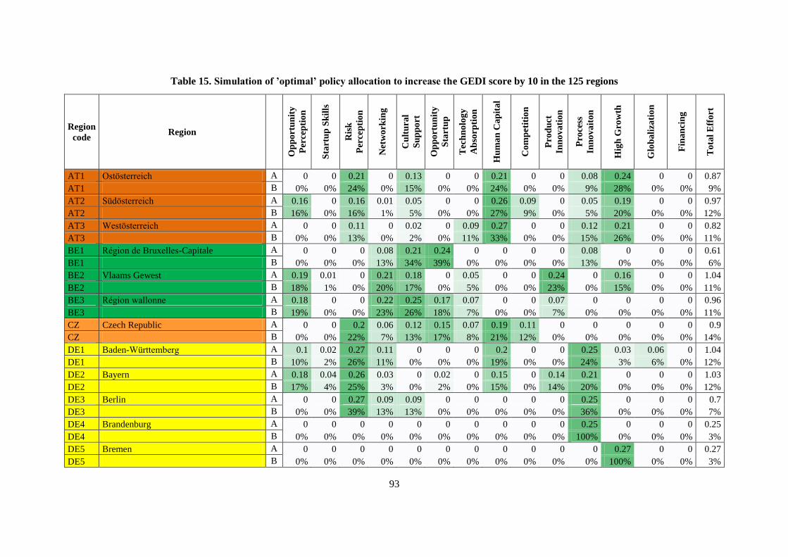
93
Table 15. Simulation of ’optimal’ policy allocation to increase the GEDI score by 10 in the 125 regions
Region
code Region
Op
po
rtu
nit
y
Per
cep
tio
n
Sta
rtu
p S
kil
ls
Ris
k
Per
cep
tio
n
Net
wo
rkin
g
Cu
ltu
ral
Su
pp
ort
Op
po
rtu
nit
y
Sta
rtu
p
Tec
hn
olo
gy
Ab
sorp
tio
n
Hu
ma
n C
ap
ita
l
Co
mp
etit
ion
Pro
du
ct
Inn
ov
ati
on
Pro
cess
Inn
ov
ait
on
Hig
h G
row
th
Glo
ba
liza
tio
n
Fin
an
cin
g
To
tal
Eff
ort
AT1 Ostösterreich A 0 0 0.21 0 0.13 0 0 0.21 0 0 0.08 0.24 0 0 0.87
AT1 B 0% 0% 24% 0% 15% 0% 0% 24% 0% 0% 9% 28% 0% 0% 9%
AT2 Südösterreich A 0.16 0 0.16 0.01 0.05 0 0 0.26 0.09 0 0.05 0.19 0 0 0.97
AT2 B 16% 0% 16% 1% 5% 0% 0% 27% 9% 0% 5% 20% 0% 0% 12%
AT3 Westösterreich A 0 0 0.11 0 0.02 0 0.09 0.27 0 0 0.12 0.21 0 0 0.82
AT3 B 0% 0% 13% 0% 2% 0% 11% 33% 0% 0% 15% 26% 0% 0% 11%
BE1 Région de Bruxelles-Capitale A 0 0 0 0.08 0.21 0.24 0 0 0 0 0.08 0 0 0 0.61
BE1 B 0% 0% 0% 13% 34% 39% 0% 0% 0% 0% 13% 0% 0% 0% 6%
BE2 Vlaams Gewest A 0.19 0.01 0 0.21 0.18 0 0.05 0 0 0.24 0 0.16 0 0 1.04
BE2 B 18% 1% 0% 20% 17% 0% 5% 0% 0% 23% 0% 15% 0% 0% 11%
BE3 Région wallonne A 0.18 0 0 0.22 0.25 0.17 0.07 0 0 0.07 0 0 0 0 0.96
BE3 B 19% 0% 0% 23% 26% 18% 7% 0% 0% 7% 0% 0% 0% 0% 11%
CZ Czech Republic A 0 0 0.2 0.06 0.12 0.15 0.07 0.19 0.11 0 0 0 0 0 0.9
CZ B 0% 0% 22% 7% 13% 17% 8% 21% 12% 0% 0% 0% 0% 0% 14%
DE1 Baden-Württemberg A 0.1 0.02 0.27 0.11 0 0 0 0.2 0 0 0.25 0.03 0.06 0 1.04
DE1 B 10% 2% 26% 11% 0% 0% 0% 19% 0% 0% 24% 3% 6% 0% 12%
DE2 Bayern A 0.18 0.04 0.26 0.03 0 0.02 0 0.15 0 0.14 0.21 0 0 0 1.03
DE2 B 17% 4% 25% 3% 0% 2% 0% 15% 0% 14% 20% 0% 0% 0% 12%
DE3 Berlin A 0 0 0.27 0.09 0.09 0 0 0 0 0 0.25 0 0 0 0.7
DE3 B 0% 0% 39% 13% 13% 0% 0% 0% 0% 0% 36% 0% 0% 0% 7%
DE4 Brandenburg A 0 0 0 0 0 0 0 0 0 0 0.25 0 0 0 0.25
DE4 B 0% 0% 0% 0% 0% 0% 0% 0% 0% 0% 100% 0% 0% 0% 3%
DE5 Bremen A 0 0 0 0 0 0 0 0 0 0 0 0.27 0 0 0.27
DE5 B 0% 0% 0% 0% 0% 0% 0% 0% 0% 0% 0% 100% 0% 0% 3%

94
Region
code Region
Op
po
rtu
nit
y
Per
cep
tio
n
Sta
rtu
p S
kil
ls
Ris
k
Per
cep
tio
n
Net
wo
rkin
g
Cu
ltu
ral
Su
pp
ort
Op
po
rtu
nit
y
Sta
rtu
p
Tec
hn
olo
gy
Ab
sorp
tio
n
Hu
ma
n C
ap
ita
l
Co
mp
etit
ion
Pro
du
ct
Inn
ov
ati
on
Pro
cess
Inn
ov
ait
on
Hig
h G
row
th
Glo
ba
liza
tio
n
Fin
an
cin
g
To
tal
Eff
ort
DE6 Hamburg A 0 0 0.02 0 0 0 0 0 0 0 0.18 0.26 0 0 0.46
DE6 B 0% 0% 4% 0% 0% 0% 0% 0% 0% 0% 39% 57% 0% 0% 5%
DE7 Hessen A 0.04 0.05 0.29 0.09 0.07 0.13 0.01 0 0 0 0.13 0 0 0 0.81
DE7 B 5% 6% 36% 11% 9% 16% 1% 0% 0% 0% 16% 0% 0% 0% 8%
DE8 Mecklenburg-Vorpommern A 0.14 0 0.01 0 0 0 0 0.22 0.06 0.18 0.14 0.23 0 0 0.98
DE8 B 14% 0% 1% 0% 0% 0% 0% 22% 6% 18% 14% 23% 0% 0% 18%
DE9 Niedersachsen A 0.25 0.11 0.24 0.03 0.01 0.02 0.04 0.18 0 0.03 0.22 0 0.01 0 1.14
DE9 B 22% 10% 21% 3% 1% 2% 4% 16% 0% 3% 19% 0% 1% 0% 15%
DEA Nordrhein-Westfalen A 0.01 0.19 0.24 0.02 0 0.02 0.03 0.1 0.12 0.1 0.21 0 0 0.1 1.14
DEA B 1% 17% 21% 2% 0% 2% 3% 9% 11% 9% 18% 0% 0% 9% 14%
DEB Rheinland-Pfalz A 0.22 0.07 0.27 0.02 0.1 0.01 0.11 0.13 0.04 0.03 0 0 0 0.06 1.06
DEB B 21% 7% 25% 2% 9% 1% 10% 12% 4% 3% 0% 0% 0% 6% 13%
DEC Saarland A 0.02 0.24 0.22 0.06 0.05 0.01 0 0.18 0.06 0 0.12 0 0 0.11 1.07
DEC B 2% 22% 21% 6% 5% 1% 0% 17% 6% 0% 11% 0% 0% 10% 13%
DED Sachsen A 0.16 0.11 0.2 0 0 0 0 0 0.01 0.27 0.14 0.17 0 0 1.06
DED B 15% 10% 19% 0% 0% 0% 0% 0% 1% 25% 13% 16% 0% 0% 14%
DEE Sachsen-Anhalt A 0.15 0 0.06 0 0 0 0 0.11 0 0 0 0.23 0 0.25 0.8
DEE B 19% 0% 8% 0% 0% 0% 0% 14% 0% 0% 0% 29% 0% 31% 12%
DEF Schleswig-Holstein A 0.1 0 0.05 0 0 0 0 0.03 0 0.3 0 0.08 0 0 0.56
DEF B 18% 0% 9% 0% 0% 0% 0% 5% 0% 54% 0% 14% 0% 0% 8%
DEG Thüringen A 0.1 0 0 0 0 0 0 0 0 0 0.26 0.28 0 0 0.64
DEG B 16% 0% 0% 0% 0% 0% 0% 0% 0% 0% 41% 44% 0% 0% 10%
DK01 Hovedstaden A 0 0.08 0.16 0 0 0 0 0 0 0 0 0 0.27 0.1 0.61
DK01 B 0% 13% 26% 0% 0% 0% 0% 0% 0% 0% 0% 0% 44% 16% 5%
DK02 Sjalland A 0 0 0 0 0 0 0 0 0 0 0 0 0.25 0 0.25
DK02 B 0% 0% 0% 0% 0% 0% 0% 0% 0% 0% 0% 0% 100% 0% 2%
DK03 Syddanmark A 0 0.14 0 0 0 0 0.08 0 0 0 0.24 0.04 0.17 0 0.67

95
Region
code Region
Op
po
rtu
nit
y
Per
cep
tio
n
Sta
rtu
p S
kil
ls
Ris
k
Per
cep
tio
n
Net
wo
rkin
g
Cu
ltu
ral
Su
pp
ort
Op
po
rtu
nit
y
Sta
rtu
p
Tec
hn
olo
gy
Ab
sorp
tio
n
Hu
ma
n C
ap
ita
l
Co
mp
etit
ion
Pro
du
ct
Inn
ov
ati
on
Pro
cess
Inn
ov
ait
on
Hig
h G
row
th
Glo
ba
liza
tio
n
Fin
an
cin
g
To
tal
Eff
ort
DK03 B 0% 21% 0% 0% 0% 0% 12% 0% 0% 0% 36% 6% 25% 0% 7%
DK04 Midtjylland A 0 0.06 0 0 0 0 0 0 0 0 0.23 0 0.2 0 0.49
DK04 B 0% 12% 0% 0% 0% 0% 0% 0% 0% 0% 47% 0% 41% 0% 5%
DK05 Nordjylland A 0 0.26 0.05 0 0 0 0 0 0 0 0 0 0.25 0 0.56
DK05 B 0% 46% 9% 0% 0% 0% 0% 0% 0% 0% 0% 0% 45% 0% 5%
EE Estonia A 0 0 0 0.13 0.23 0.13 0.04 0 0.05 0.01 0 0 0 0.28 0.87
EE B 0% 0% 0% 15% 26% 15% 5% 0% 6% 1% 0% 0% 0% 32% 12%
EL1 Voreia Ellada A 0 0 0.24 0.1 0.26 0.2 0.01 0 0.08 0 0 0.08 0 0 0.97
EL1 B 0% 0% 25% 10% 27% 21% 1% 0% 8% 0% 0% 8% 0% 0% 26%
EL2 Kentriki Ellada A 0.04 0.05 0.21 0.1 0.21 0.12 0.04 0.03 0.12 0 0 0.15 0.08 0 1.15
EL2 B 3% 4% 18% 9% 18% 10% 3% 3% 10% 0% 0% 13% 7% 0% 37%
EL3 Attiki A 0 0 0.27 0.08 0.28 0.02 0 0 0.06 0 0 0.01 0 0 0.72
EL3 B 0% 0% 38% 11% 39% 3% 0% 0% 8% 0% 0% 1% 0% 0% 14%
EL4 Nisia Aigaiou. Kriti A 0.02 0 0.23 0.07 0.24 0.08 0.06 0.07 0.08 0 0 0.15 0.05 0 1.05
EL4 B 2% 0% 22% 7% 23% 8% 6% 7% 8% 0% 0% 14% 5% 0% 30%
ES11 Galicia A 0.13 0.07 0.1 0.09 0 0 0 0 0.15 0 0.01 0.23 0.23 0.12 1.13
ES11 B 12% 6% 9% 8% 0% 0% 0% 0% 13% 0% 1% 20% 20% 11% 21%
ES12 Principado de Asturias A 0.1 0.16 0.14 0.12 0 0 0 0 0.15 0 0 0.19 0.22 0.07 1.15
ES12 B 9% 14% 12% 10% 0% 0% 0% 0% 13% 0% 0% 17% 19% 6% 18%
ES13 Cantabria A 0.1 0.09 0.09 0.03 0 0.01 0 0 0.08 0 0.08 0.25 0.21 0.16 1.1
ES13 B 9% 8% 8% 3% 0% 1% 0% 0% 7% 0% 7% 23% 19% 15% 20%
ES21 País Vasco A 0 0.03 0.09 0.09 0 0 0 0 0.18 0.07 0 0.2 0.25 0 0.91
ES21 B 0% 3% 10% 10% 0% 0% 0% 0% 20% 8% 0% 22% 27% 0% 13%
ES22 Comunidad Foral de Navarra A 0.09 0.06 0.07 0.06 0 0 0.01 0 0.17 0.02 0 0.21 0.26 0 0.95
ES22 B 9% 6% 7% 6% 0% 0% 1% 0% 18% 2% 0% 22% 27% 0% 16%
ES23 La Rioja A 0.07 0.12 0.06 0.04 0 0 0 0 0.15 0.12 0 0.21 0.24 0.02 1.03
ES23 B 7% 12% 6% 4% 0% 0% 0% 0% 15% 12% 0% 20% 23% 2% 18%
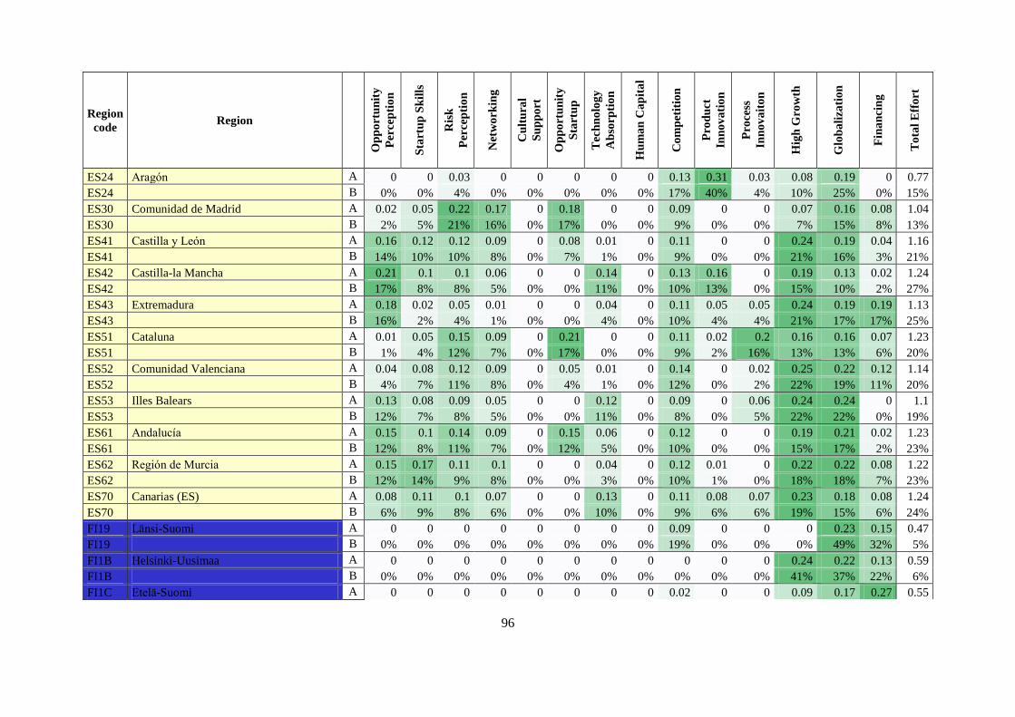
96
Region
code Region
Op
po
rtu
nit
y
Per
cep
tio
n
Sta
rtu
p S
kil
ls
Ris
k
Per
cep
tio
n
Net
wo
rkin
g
Cu
ltu
ral
Su
pp
ort
Op
po
rtu
nit
y
Sta
rtu
p
Tec
hn
olo
gy
Ab
sorp
tio
n
Hu
ma
n C
ap
ita
l
Co
mp
etit
ion
Pro
du
ct
Inn
ov
ati
on
Pro
cess
Inn
ov
ait
on
Hig
h G
row
th
Glo
ba
liza
tio
n
Fin
an
cin
g
To
tal
Eff
ort
ES24 Aragón A 0 0 0.03 0 0 0 0 0 0.13 0.31 0.03 0.08 0.19 0 0.77
ES24 B 0% 0% 4% 0% 0% 0% 0% 0% 17% 40% 4% 10% 25% 0% 15%
ES30 Comunidad de Madrid A 0.02 0.05 0.22 0.17 0 0.18 0 0 0.09 0 0 0.07 0.16 0.08 1.04
ES30 B 2% 5% 21% 16% 0% 17% 0% 0% 9% 0% 0% 7% 15% 8% 13%
ES41 Castilla y León A 0.16 0.12 0.12 0.09 0 0.08 0.01 0 0.11 0 0 0.24 0.19 0.04 1.16
ES41 B 14% 10% 10% 8% 0% 7% 1% 0% 9% 0% 0% 21% 16% 3% 21%
ES42 Castilla-la Mancha A 0.21 0.1 0.1 0.06 0 0 0.14 0 0.13 0.16 0 0.19 0.13 0.02 1.24
ES42 B 17% 8% 8% 5% 0% 0% 11% 0% 10% 13% 0% 15% 10% 2% 27%
ES43 Extremadura A 0.18 0.02 0.05 0.01 0 0 0.04 0 0.11 0.05 0.05 0.24 0.19 0.19 1.13
ES43 B 16% 2% 4% 1% 0% 0% 4% 0% 10% 4% 4% 21% 17% 17% 25%
ES51 Cataluna A 0.01 0.05 0.15 0.09 0 0.21 0 0 0.11 0.02 0.2 0.16 0.16 0.07 1.23
ES51 B 1% 4% 12% 7% 0% 17% 0% 0% 9% 2% 16% 13% 13% 6% 20%
ES52 Comunidad Valenciana A 0.04 0.08 0.12 0.09 0 0.05 0.01 0 0.14 0 0.02 0.25 0.22 0.12 1.14
ES52 B 4% 7% 11% 8% 0% 4% 1% 0% 12% 0% 2% 22% 19% 11% 20%
ES53 Illes Balears A 0.13 0.08 0.09 0.05 0 0 0.12 0 0.09 0 0.06 0.24 0.24 0 1.1
ES53 B 12% 7% 8% 5% 0% 0% 11% 0% 8% 0% 5% 22% 22% 0% 19%
ES61 Andalucía A 0.15 0.1 0.14 0.09 0 0.15 0.06 0 0.12 0 0 0.19 0.21 0.02 1.23
ES61 B 12% 8% 11% 7% 0% 12% 5% 0% 10% 0% 0% 15% 17% 2% 23%
ES62 Región de Murcia A 0.15 0.17 0.11 0.1 0 0 0.04 0 0.12 0.01 0 0.22 0.22 0.08 1.22
ES62 B 12% 14% 9% 8% 0% 0% 3% 0% 10% 1% 0% 18% 18% 7% 23%
ES70 Canarias (ES) A 0.08 0.11 0.1 0.07 0 0 0.13 0 0.11 0.08 0.07 0.23 0.18 0.08 1.24
ES70 B 6% 9% 8% 6% 0% 0% 10% 0% 9% 6% 6% 19% 15% 6% 24%
FI19 Länsi-Suomi A 0 0 0 0 0 0 0 0 0.09 0 0 0 0.23 0.15 0.47
FI19 B 0% 0% 0% 0% 0% 0% 0% 0% 19% 0% 0% 0% 49% 32% 5%
FI1B Helsinki-Uusimaa A 0 0 0 0 0 0 0 0 0 0 0 0.24 0.22 0.13 0.59
FI1B B 0% 0% 0% 0% 0% 0% 0% 0% 0% 0% 0% 41% 37% 22% 6%
FI1C Etelä-Suomi A 0 0 0 0 0 0 0 0 0.02 0 0 0.09 0.17 0.27 0.55
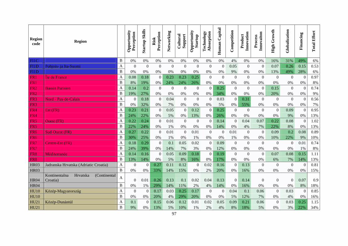
97
Region
code Region
Op
po
rtu
nit
y
Per
cep
tio
n
Sta
rtu
p S
kil
ls
Ris
k
Per
cep
tio
n
Net
wo
rkin
g
Cu
ltu
ral
Su
pp
ort
Op
po
rtu
nit
y
Sta
rtu
p
Tec
hn
olo
gy
Ab
sorp
tio
n
Hu
ma
n C
ap
ita
l
Co
mp
etit
ion
Pro
du
ct
Inn
ov
ati
on
Pro
cess
Inn
ov
ait
on
Hig
h G
row
th
Glo
ba
liza
tio
n
Fin
an
cin
g
To
tal
Eff
ort
FI1C B 0% 0% 0% 0% 0% 0% 0% 0% 4% 0% 0% 16% 31% 49% 6%
FI1D Pohjois- ja Ita-Suomi A 0 0 0 0 0 0 0 0 0.05 0 0 0.07 0.26 0.15 0.53
FI1D B 0% 0% 0% 0% 0% 0% 0% 0% 9% 0% 0% 13% 49% 28% 6%
FR1 Île de France A 0.08 0.18 0 0.23 0.23 0.25 0 0 0 0 0 0 0 0 0.97
FR1 B 8% 19% 0% 24% 24% 26% 0% 0% 0% 0% 0% 0% 0% 0% 8%
FR2 Bassin Parisien A 0.14 0.2 0 0 0 0 0 0.25 0 0 0 0.15 0 0 0.74
FR2 B 19% 27% 0% 0% 0% 0% 0% 34% 0% 0% 0% 20% 0% 0% 9%
FR3 Nord - Pas-de-Calais A 0 0.18 0 0.04 0 0 0 0.03 0 0.31 0 0 0 0 0.56
FR3 B 0% 32% 0% 7% 0% 0% 0% 5% 0% 55% 0% 0% 0% 0% 7%
FR4 Est (FR) A 0.23 0.21 0 0.05 0 0.12 0 0.25 0 0 0 0 0.09 0 0.95
FR4 B 24% 22% 0% 5% 0% 13% 0% 26% 0% 0% 0% 0% 9% 0% 13%
FR5 Ouest (FR) A 0.22 0.24 0 0.01 0 0 0 0.14 0 0.04 0.07 0.22 0.08 0 1.02
FR5 B 22% 24% 0% 1% 0% 0% 0% 14% 0% 4% 7% 22% 8% 0% 13%
FR6 Sud-Ouest (FR) A 0.27 0.22 0 0.01 0 0.01 0 0 0.01 0 0 0.09 0.2 0.08 0.89
FR6 B 30% 25% 0% 1% 0% 1% 0% 0% 1% 0% 0% 10% 22% 9% 10%
FR7 Centre-Est (FR) A 0.18 0.29 0 0.1 0.05 0.02 0 0.09 0 0 0 0 0 0.01 0.74
FR7 B 24% 39% 0% 14% 7% 3% 0% 12% 0% 0% 0% 0% 0% 1% 8%
FR8 Méditerranée A 0.14 0.16 0 0.05 0.09 0.18 0 0.19 0 0 0 0.07 0.08 0.15 1.11
FR8 B 13% 14% 0% 5% 8% 16% 0% 17% 0% 0% 0% 6% 7% 14% 13%
HR03 Jadranska Hrvatska (Adriatic Croatia) A 0 0 0.27 0.11 0.12 0 0.02 0.16 0 0.13 0 0 0 0 0.81
HR03 B 0% 0% 33% 14% 15% 0% 2% 20% 0% 16% 0% 0% 0% 0% 15%
HR04
Kontinentalna Hrvatska (Continental
Croatia) A
0 0.01 0.26 0.13 0.1 0.02 0.04 0.13 0 0.14 0 0 0 0.07 0.9
HR04 B 0% 1% 29% 14% 11% 2% 4% 14% 0% 16% 0% 0% 0% 8% 18%
HU10 Közép-Magyarország A 0 0 0.17 0.03 0.25 0.17 0 0 0.04 0.1 0.06 0 0.03 0 0.85
HU10 B 0% 0% 20% 4% 29% 20% 0% 0% 5% 12% 7% 0% 4% 0% 16%
HU21 Közép-Dunántúl A 0.1 0 0.15 0.06 0.12 0.01 0.02 0.05 0.09 0.21 0.06 0 0.03 0.25 1.15
HU21 B 9% 0% 13% 5% 10% 1% 2% 4% 8% 18% 5% 0% 3% 22% 34%

98
Region
code Region
Op
po
rtu
nit
y
Per
cep
tio
n
Sta
rtu
p S
kil
ls
Ris
k
Per
cep
tio
n
Net
wo
rkin
g
Cu
ltu
ral
Su
pp
ort
Op
po
rtu
nit
y
Sta
rtu
p
Tec
hn
olo
gy
Ab
sorp
tio
n
Hu
ma
n C
ap
ita
l
Co
mp
etit
ion
Pro
du
ct
Inn
ov
ati
on
Pro
cess
Inn
ov
ait
on
Hig
h G
row
th
Glo
ba
liza
tio
n
Fin
an
cin
g
To
tal
Eff
ort
HU22 Nyugat-Dunántúl A 0 0 0.16 0.06 0.12 0 0 0.01 0.13 0.26 0.15 0.04 0 0.2 1.13
HU22 B 0% 0% 14% 5% 11% 0% 0% 1% 12% 23% 13% 4% 0% 18% 34%
HU23 Dél-Dunántúl A 0.1 0 0.17 0.06 0.14 0 0.06 0.07 0.13 0.11 0.09 0 0 0.24 1.17
HU23 B 9% 0% 15% 5% 12% 0% 5% 6% 11% 9% 8% 0% 0% 21% 32%
HU31 Észak-Magyarország A 0.07 0 0.16 0.07 0.13 0.03 0 0.06 0.06 0.22 0.07 0 0.09 0.21 1.17
HU31 B 6% 0% 14% 6% 11% 3% 0% 5% 5% 19% 6% 0% 8% 18% 33%
HU32 Észak-Alföld A 0.16 0 0.17 0.1 0.14 0.05 0 0.09 0.1 0.17 0 0 0.06 0.22 1.26
HU32 B 13% 0% 13% 8% 11% 4% 0% 7% 8% 13% 0% 0% 5% 17% 40%
HU33 Dél-Alföld A 0.14 0 0.16 0.09 0.14 0.07 0.07 0.12 0.11 0.11 0.06 0 0.03 0.19 1.29
HU33 B 11% 0% 12% 7% 11% 5% 5% 9% 9% 9% 5% 0% 2% 15% 42%
IE01 Border. Midland and Western A 0.19 0 0 0.06 0 0.1 0.01 0 0.1 0.29 0.06 0 0.05 0.07 0.93
IE01 B 20% 0% 0% 6% 0% 11% 1% 0% 11% 31% 6% 0% 5% 8% 10%
IE02 Southern and Eastern A 0.21 0 0 0.04 0.05 0.16 0.08 0 0 0.03 0.08 0.04 0.26 0.05 1
IE02 B 21% 0% 0% 4% 5% 16% 8% 0% 0% 3% 8% 4% 26% 5% 10%
ITC Nord-Ovest A 0 0.07 0 0.21 0.1 0.19 0 0.26 0 0.1 0.02 0 0 0 0.95
ITC B 0% 7% 0% 22% 11% 20% 0% 27% 0% 11% 2% 0% 0% 0% 15%
ITF Sud A 0 0 0 0.06 0.12 0.3 0 0.11 0 0 0 0.02 0.09 0 0.7
ITF B 0% 0% 0% 9% 17% 43% 0% 16% 0% 0% 0% 3% 13% 0% 15%
ITG Isole A 0.02 0 0 0.1 0.1 0.29 0.08 0.12 0 0.04 0 0.04 0.05 0.04 0.88
ITG B 2% 0% 0% 11% 11% 33% 9% 14% 0% 5% 0% 5% 6% 5% 20%
ITH Nord-Est A 0.02 0.08 0 0.14 0.03 0.11 0.01 0.17 0 0 0 0.27 0.2 0 1.03
ITH B 2% 8% 0% 14% 3% 11% 1% 17% 0% 0% 0% 26% 19% 0% 19%
ITI Centro (IT) A 0.02 0.04 0 0.17 0.11 0.25 0.03 0.19 0 0.02 0 0.13 0.07 0 1.03
ITI B 2% 4% 0% 17% 11% 24% 3% 18% 0% 2% 0% 13% 7% 0% 18%
LT Lithuania A 0 0 0 0.14 0.15 0.22 0.11 0 0.15 0.15 0 0 0 0.07 0.99
LT B 0% 0% 0% 14% 15% 22% 11% 0% 15% 15% 0% 0% 0% 7% 18%
LV Latvia A 0 0 0 0.18 0.19 0.21 0.09 0 0.03 0.2 0.11 0 0 0.09 1.1
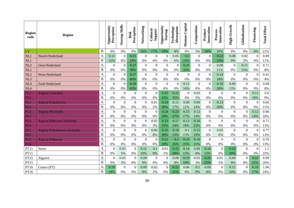
99
Region
code Region
Op
po
rtu
nit
y
Per
cep
tio
n
Sta
rtu
p S
kil
ls
Ris
k
Per
cep
tio
n
Net
wo
rkin
g
Cu
ltu
ral
Su
pp
ort
Op
po
rtu
nit
y
Sta
rtu
p
Tec
hn
olo
gy
Ab
sorp
tio
n
Hu
ma
n C
ap
ita
l
Co
mp
etit
ion
Pro
du
ct
Inn
ov
ati
on
Pro
cess
Inn
ov
ait
on
Hig
h G
row
th
Glo
ba
liza
tio
n
Fin
an
cin
g
To
tal
Eff
ort
LV B 0% 0% 0% 16% 17% 19% 8% 0% 3% 18% 10% 0% 0% 8% 21%
NL1 Noord-Nederland A 0.11 0 0.21 0 0 0 0.05 0.2 0 0 0.22 0.08 0.02 0 0.89
NL1 B 12% 0% 24% 0% 0% 0% 6% 22% 0% 0% 25% 9% 2% 0% 11%
NL2 Oost-Nederland A 0 0 0.27 0 0 0 0 0.25 0 0 0.08 0 0.11 0 0.71
NL2 B 0% 0% 38% 0% 0% 0% 0% 35% 0% 0% 11% 0% 15% 0% 8%
NL3 West-Nederland A 0 0 0.27 0 0 0 0 0 0 0 0.14 0 0 0 0.41
NL3 B 0% 0% 66% 0% 0% 0% 0% 0% 0% 0% 34% 0% 0% 0% 4%
NL4 Zuid-Nederland A 0 0 0.29 0 0 0 0 0.11 0 0 0.19 0.09 0 0 0.68
NL4 B 0% 0% 43% 0% 0% 0% 0% 16% 0% 0% 28% 13% 0% 0% 8%
PL1 Region Centralny A 0 0 0 0 0 0.25 0.21 0 0.03 0 0 0 0 0.11 0.6
PL1 B 0% 0% 0% 0% 0% 42% 35% 0% 5% 0% 0% 0% 0% 18% 9%
PL2 Region Poludniowy A 0 0 0 0 0.01 0.24 0.11 0.08 0.09 0 0.13 0 0 0 0.66
PL2 B 0% 0% 0% 0% 2% 36% 17% 12% 14% 0% 20% 0% 0% 0% 11%
PL3 Region Wschodni A 0 0 0 0 0 0.24 0.23 0.15 0.12 0 0 0 0 0.12 0.86
PL3 B 0% 0% 0% 0% 0% 28% 27% 17% 14% 0% 0% 0% 0% 14% 18%
PL4 Region Pólnocno-Zachodni A 0 0 0 0 0.02 0.23 0.17 0.13 0.16 0 0 0 0 0 0.71
PL4 B 0% 0% 0% 0% 3% 32% 24% 18% 23% 0% 0% 0% 0% 0% 13%
PL5 Region Poludniowo-Zachodni A 0 0 0 0 0.06 0.23 0.18 0.1 0.15 0 0.05 0 0 0 0.77
PL5 B 0% 0% 0% 0% 8% 30% 23% 13% 19% 0% 6% 0% 0% 0% 13%
PL6 Region Pólnocny A 0 0 0 0 0 0.21 0.2 0.19 0.16 0 0 0 0 0 0.76
PL6 B 0% 0% 0% 0% 0% 28% 26% 25% 21% 0% 0% 0% 0% 0% 13%
PT11 Norte A 0 0.05 0 0.11 0.1 0.01 0.22 0.14 0.09 0.16 0 0.22 0 0 1.1
PT11 B 0% 5% 0% 10% 9% 1% 20% 13% 8% 15% 0% 20% 0% 0% 25%
PT15 Algarve A 0 0.03 0 0.09 0 0 0.08 0.19 0.03 0.25 0.01 0.09 0 0.22 0.99
PT15 B 0% 3% 0% 9% 0% 0% 8% 19% 3% 25% 1% 9% 0% 22% 20%
PT16 Centro (PT) A 0.19 0 0 0.09 0.02 0 0.22 0.06 0.1 0.09 0 0.11 0 0.18 1.06
PT16 B 18% 0% 0% 8% 2% 0% 21% 6% 9% 8% 0% 10% 0% 17% 24%

100
Region
code Region
Op
po
rtu
nit
y
Per
cep
tio
n
Sta
rtu
p S
kil
ls
Ris
k
Per
cep
tio
n
Net
wo
rkin
g
Cu
ltu
ral
Su
pp
ort
Op
po
rtu
nit
y
Sta
rtu
p
Tec
hn
olo
gy
Ab
sorp
tio
n
Hu
ma
n C
ap
ita
l
Co
mp
etit
ion
Pro
du
ct
Inn
ov
ati
on
Pro
cess
Inn
ov
ait
on
Hig
h G
row
th
Glo
ba
liza
tio
n
Fin
an
cin
g
To
tal
Eff
ort
PT17 Lisboa A 0 0 0 0.2 0.14 0.08 0.27 0 0.1 0.12 0 0 0 0 0.91
PT17 B 0% 0% 0% 22% 15% 9% 30% 0% 11% 13% 0% 0% 0% 0% 13%
PT18 Alentejo A 0 0 0 0.04 0 0 0.26 0.06 0.04 0.18 0 0 0 0.19 0.77
PT18 B 0% 0% 0% 5% 0% 0% 34% 8% 5% 23% 0% 0% 0% 25% 15%
RO1 Macroregiunea unu A 0 0.21 0 0.16 0.1 0.16 0.11 0.01 0.04 0.22 0 0.01 0 0.08 1.1
RO1 B 0% 19% 0% 15% 9% 15% 10% 1% 4% 20% 0% 1% 0% 7% 34%
RO2 Macroregiunea doi A 0 0.2 0 0.16 0.17 0.21 0.13 0.07 0.04 0.08 0 0 0 0 1.06
RO2 B 0% 19% 0% 15% 16% 20% 12% 7% 4% 8% 0% 0% 0% 0% 33%
RO3 Macroregiunea trei A 0 0.17 0 0.12 0.18 0.21 0.03 0 0.04 0.12 0 0 0 0.09 0.96
RO3 B 0% 18% 0% 13% 19% 22% 3% 0% 4% 13% 0% 0% 0% 9% 24%
RO4 Macroregiunea patru A 0 0.19 0 0.14 0.13 0.2 0.05 0 0.04 0.19 0 0 0 0.13 1.07
RO4 B 0% 18% 0% 13% 12% 19% 5% 0% 4% 18% 0% 0% 0% 12% 31%
SE11 Stockholm A 0 0 0 0 0 0 0 0 0.04 0 0.19 0.26 0.08 0 0.57
SE11 B 0% 0% 0% 0% 0% 0% 0% 0% 7% 0% 33% 46% 14% 0% 5%
SE12 Östra Mellansverige A 0 0.12 0 0 0 0 0.14 0.18 0.2 0 0.2 0 0.19 0 1.03
SE12 B 0% 12% 0% 0% 0% 0% 14% 17% 19% 0% 19% 0% 18% 0% 10%
SE21 Smaland med öarna A 0 0 0 0 0 0 0.05 0.07 0 0.21 0.17 0.22 0.09 0 0.81
SE21 B 0% 0% 0% 0% 0% 0% 6% 9% 0% 26% 21% 27% 11% 0% 10%
SE22 Sydsverige A 0 0 0 0 0 0 0.08 0 0.05 0.1 0.29 0 0.12 0 0.64
SE22 B 0% 0% 0% 0% 0% 0% 13% 0% 8% 16% 45% 0% 19% 0% 6%
SE23 Vastsverige A 0 0.08 0 0 0 0 0.17 0 0.11 0.22 0 0.18 0.21 0.02 0.99
SE23 B 0% 8% 0% 0% 0% 0% 17% 0% 11% 22% 0% 18% 21% 2% 9%
SE31 Norra Mellansverige A 0 0.02 0 0 0 0 0.06 0 0.15 0.23 0.16 0.16 0.08 0 0.86
SE31 B 0% 2% 0% 0% 0% 0% 7% 0% 17% 27% 19% 19% 9% 0% 10%
SE32 Mellersta Norrland A 0 0 0 0 0 0 0 0 0 0.02 0.12 0.22 0 0 0.36
SE32 B 0% 0% 0% 0% 0% 0% 0% 0% 0% 6% 33% 61% 0% 0% 4%
SE33 Övre Norrland A 0 0 0 0 0 0 0.26 0 0.04 0.01 0 0.24 0.17 0 0.72

101
Region
code Region
Op
po
rtu
nit
y
Per
cep
tio
n
Sta
rtu
p S
kil
ls
Ris
k
Per
cep
tio
n
Net
wo
rkin
g
Cu
ltu
ral
Su
pp
ort
Op
po
rtu
nit
y
Sta
rtu
p
Tec
hn
olo
gy
Ab
sorp
tio
n
Hu
ma
n C
ap
ita
l
Co
mp
etit
ion
Pro
du
ct
Inn
ov
ati
on
Pro
cess
Inn
ov
ait
on
Hig
h G
row
th
Glo
ba
liza
tio
n
Fin
an
cin
g
To
tal
Eff
ort
SE33 B 0% 0% 0% 0% 0% 0% 36% 0% 6% 1% 0% 33% 24% 0% 7%
SI01 Vzhodna Slovenija A 0.1 0.06 0.28 0.02 0.01 0.13 0.04 0.08 0.21 0 0 0 0 0.07 1
SI01 B 10% 6% 28% 2% 1% 13% 4% 8% 21% 0% 0% 0% 0% 7% 15%
SI02 Zahodna Slovenija A 0.02 0 0.28 0 0.05 0.16 0 0 0.12 0 0 0.02 0 0.17 0.82
SI02 B 2% 0% 34% 0% 6% 20% 0% 0% 15% 0% 0% 2% 0% 21% 10%
SK01 Bratislavsky kraj A 0 0 0.07 0 0.24 0.06 0 0 0.03 0 0 0 0 0 0.4
SK01 B 0% 0% 18% 0% 60% 15% 0% 0% 8% 0% 0% 0% 0% 0% 5%
SK02 Západné Slovensko A 0.08 0 0.07 0 0.22 0.12 0 0.15 0.16 0.17 0 0 0 0 0.97
SK02 B 8% 0% 7% 0% 23% 12% 0% 15% 16% 18% 0% 0% 0% 0% 22%
SK03 Stredné Slovensko A 0.1 0 0.06 0 0.21 0.12 0.06 0.13 0.15 0.18 0 0 0 0 1.01
SK03 B 10% 0% 6% 0% 21% 12% 6% 13% 15% 18% 0% 0% 0% 0% 25%
SK04 Vychodné Slovensko A 0.07 0.04 0.07 0 0.22 0.13 0.11 0.16 0.15 0.02 0 0 0 0 0.97
SK04 B 7% 4% 7% 0% 23% 13% 11% 16% 15% 2% 0% 0% 0% 0% 24%
UKC North East (UK) A 0 0 0 0 0 0 0 0 0 0 0.16 0 0.28 0.2 0.64
UKC B 0% 0% 0% 0% 0% 0% 0% 0% 0% 0% 25% 0% 44% 31% 8%
UKD North West (UK) A 0 0.03 0 0.06 0 0 0 0.06 0 0.14 0.04 0 0.22 0.28 0.83
UKD B 0% 4% 0% 7% 0% 0% 0% 7% 0% 17% 5% 0% 27% 34% 9%
UKE Yorkshire and The Humber A 0 0.02 0 0.03 0 0 0 0.08 0 0.15 0.26 0 0.27 0.1 0.91
UKE B 0% 2% 0% 3% 0% 0% 0% 9% 0% 16% 29% 0% 30% 11% 11%
UKF East Midlands (UK) A 0.05 0.02 0 0 0 0 0 0.06 0 0.27 0.15 0.05 0.23 0.1 0.93
UKF B 5% 2% 0% 0% 0% 0% 0% 6% 0% 29% 16% 5% 25% 11% 11%
UKG West Midlands (UK) A 0.02 0.06 0 0.1 0 0 0 0.08 0 0.19 0.22 0 0.15 0.24 1.06
UKG B 2% 6% 0% 9% 0% 0% 0% 8% 0% 18% 21% 0% 14% 23% 12%
UKH East of England A 0.09 0 0 0.04 0.02 0 0 0.18 0 0.01 0 0 0.19 0.28 0.81
UKH B 11% 0% 0% 5% 2% 0% 0% 22% 0% 1% 0% 0% 23% 35% 9%
UKI London A 0 0 0 0.12 0.19 0.24 0 0 0 0.07 0.18 0 0 0.14 0.94
UKI B 0% 0% 0% 13% 20% 26% 0% 0% 0% 7% 19% 0% 0% 15% 8%

102
Region
code Region
Op
po
rtu
nit
y
Per
cep
tio
n
Sta
rtu
p S
kil
ls
Ris
k
Per
cep
tio
n
Net
wo
rkin
g
Cu
ltu
ral
Su
pp
ort
Op
po
rtu
nit
y
Sta
rtu
p
Tec
hn
olo
gy
Ab
sorp
tio
n
Hu
ma
n C
ap
ita
l
Co
mp
etit
ion
Pro
du
ct
Inn
ov
ati
on
Pro
cess
Inn
ov
ait
on
Hig
h G
row
th
Glo
ba
liza
tio
n
Fin
an
cin
g
To
tal
Eff
ort
UKJ South East (UK) A 0.08 0 0 0.06 0.03 0 0 0.02 0 0.26 0.19 0 0.13 0.15 0.92
UKJ B 9% 0% 0% 7% 3% 0% 0% 2% 0% 28% 21% 0% 14% 16% 9%
UKK South West (UK) A 0.18 0.02 0 0.01 0 0 0.03 0.06 0 0.14 0.15 0.02 0.26 0.13 1
UKK B 18% 2% 0% 1% 0% 0% 3% 6% 0% 14% 15% 2% 26% 13% 11%
UKL Wales A 0.13 0.06 0 0.02 0 0 0 0 0 0.13 0.21 0 0.14 0.26 0.95
UKL B 14% 6% 0% 2% 0% 0% 0% 0% 0% 14% 22% 0% 15% 27% 12%
UKM Scotland A 0.1 0.02 0 0 0 0 0 0 0 0.19 0.13 0 0.1 0.25 0.79
UKM B 13% 3% 0% 0% 0% 0% 0% 0% 0% 24% 16% 0% 13% 32% 9%
UKN Northern Ireland (UK) A 0.11 0.13 0 0.13 0 0 0.03 0.17 0 0.11 0.14 0 0.19 0.17 1.18
UKN B 9% 11% 0% 11% 0% 0% 3% 14% 0% 9% 12% 0% 16% 14% 14%
Legend: A = required increase in pillar; B = percentage of total effort.

103
The ‘urgency’ of action relative to different pillars can be inferred from the relative effort required to
produce a 10-point increase in the REDI index score: the higher the relative effort required (as
percentage of total additional policy effort to produce a 10-point score increase), the more ‘urgent’ that
bottleneck can be tought to be, as a pressing bottleneck prevents the system from fully leveraging all
of its strengths. In Table 16 we categorize the pillars and classify the policy actions for each
region according to the ‘urgency’ of action suggested by our simulation.
In Table 16 we categorize the pillars and classify the policy actions for each region according
to the ‘urgency’ of action suggested by our simulation.
Table 16. Urgency of bottleneck alleviation implied by the portfolio simulation
% of required
resource allocation/
Affected regions
All regions in the
country
More than 50% of
the regions in the
country
25- 50 percent of
the regions in the
country
1-25 percent of the
regions in the country
15 percent and up Top national
priority
Top regional
priority
Medium regional
priority
Low regional priority
10-14 percent Top national
priority
Medium regional
priority
Medium regional
priority
Low regional priority
5-9 percent Medium national
priority
Low regional
priority
Low regional
priority
Watch list
3- 5 percent Low national
priority
Watch list Watch list Watch list
While perfect categorization is not possible because of the large number of variations, this
approach still provides a useful implication of the magnitude of the bottleneck caused by a
particular pillar within a given system. In the following we use this categorization to discuss
each of the 24 countries included in the REDI index. It is important to remember that
bottlenecks are identified and evaluated not on an absolute but on a relative basis, as
compared to the other pillar values in the same region. So, it could happen that a region with
high REDI score could have a bottleneck pillar value of around 0.60 - for example, the Íle de
France’s lowest pillar score is 0.59 for Opportunity perception - that could equal the best
pillar score for a less developed region – e.g., the Greek Kentriki Ellada’s highest individual
pillar value is Financing with 0.59 pillar score.
Austria
Austria’s three NUTS-1 regions are listed in the first part of ranking with relatively high
REDI scores between 60.7 (Ostösterreich) and 50.3 (Westösterreich). The entrepreneurial
profiles of the three regions are rather homogeneous with respect to bottleneck pillars. Human
capital, Risk perception, and High growth are the weakest pillars that our simulation suggests
as top country-wide policy priorities. Process innovation is categorized as medium level
country wide priority. Cultural support constitutes a bottleneck in two out of the three
Austrian regions, Ostösterreich and Sudösterreich, so this pillar is indicated as the top regional
policy priority. Opportunity perception and Technology absorption score relatively low in

104
Südösterreich and Westösterrech, respectively (low policy priority). Moreover, Südösterrech
should pay attention to its Competitiveness pillar (watch list).
Belgium
Belgium has three NUTS1 regions that perform rather similarly. The leading Région de
Bruxelles-Capitale is ranked at the 13th
place while Région wallonne is at the 26th
place in the
overall REDI ranking. The REDI score differences are also minimal, between 64.9 and 60.1.
Country-wide problems can be found in two attitude pillars, Cultural support and Networking.
These bottlenecks appear to require country-wide policy action. Opportunity startup is the
weakest pillar of Région de Bruxelles-Capitale, and it is also a binding constraint for Region
Wallonne. Opportunity perception score is acceptable in the case of Région de Bruxelles-
Capitale, but not for the other two regions. Therefore regional policy should address these two
pillars in the affected regions (top priority). Product innovation is particularly low in Vlaams
Gewest and relatively week in Region Wallonne (medium-level regional policy priority).
Process innovation is problematic for Région de Bruxelles-Capitale, and High growth is for
Vlaams Gewest (low priority). Moreover, Vlaams Gewest should pay attention to Startup
skills. The most developed Région de Bruxelles-Capitale requires the least additional policy
effort (0.61) to improve its REDI score by 10 points.
Czech Republic
The Czech Republic consists of only one NUTS1 region, so we do not have the possibility to
carry out a regional level analysis. The overall entrepreneurial performance of the country is
fair with a REDI score of 37.0 – similar to the Spanish and German regions. There are three
pillars, Risk perception, Human capital and Opportunity startup that are the most binding
constraints requiring altogether 60 percent of the additional policy effort to increase the REDI
index score by 10 points. Cultural support and Competition are in the medium level policy
priority category. Technology absorption and Networking are also amongst the least binding
constraints. The Czech Republic performs particularly strongly in aspirations related pillars.
Croatia
Croatia, the newest EU member state, has only two NUTS1 regions that have a very similar
entrepreneurship level and profile with REDI scores of 32.0 (Jadranska Hrvatska) and 29.9
(Kontinentalna Hrvatska) respectively. At the NUTS1 level it is not worth discussing regional
policy in Croatia; national level policy measures are necessary. The most binding constraints
are Risk perception and Product innovation. However, Human capital, Networking and
Cultural support all appear to require policy intervention (top priority). Technology
absorption and Finance should be on the watch list.
Denmark
Danish NUTS2 regions are amongst the most entrepreneurial EU regions. In fact Hovedstaden
ranks as number one and the worst Danish region, Sjalland ranks at the 23rd
place with a still
impressive score of 60.7. According to Table 15, seven out of the fourteen pillars perform
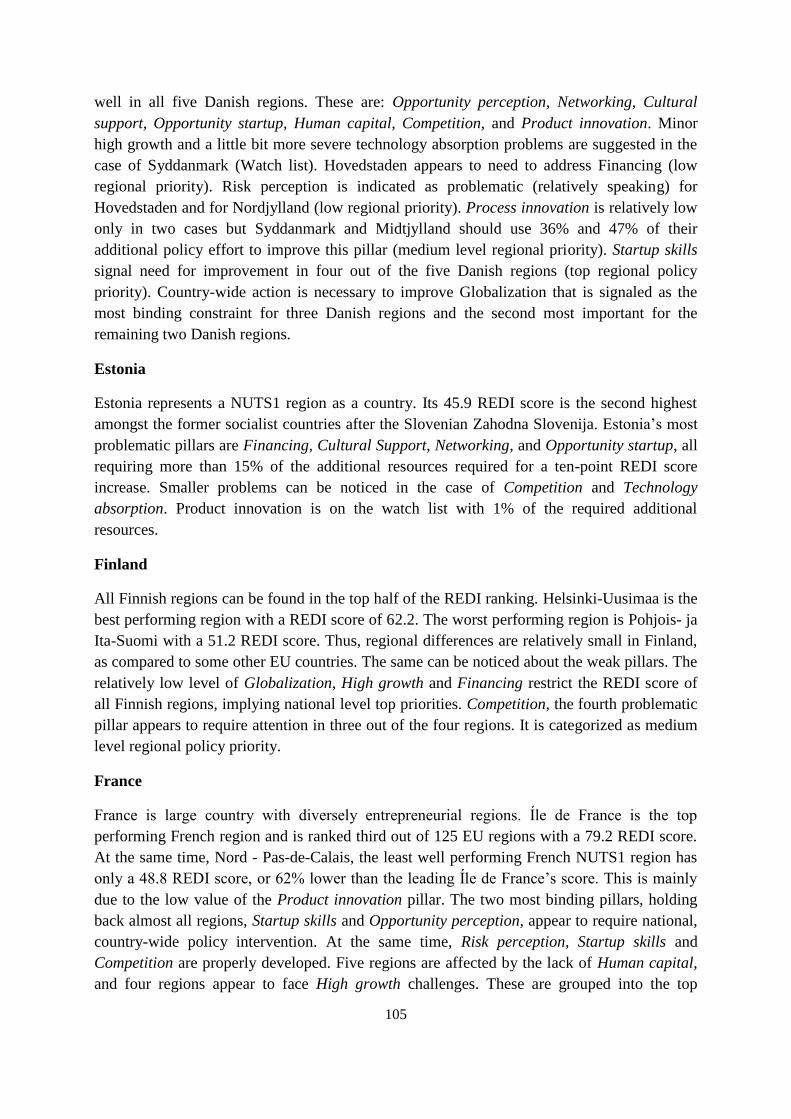
105
well in all five Danish regions. These are: Opportunity perception, Networking, Cultural
support, Opportunity startup, Human capital, Competition, and Product innovation. Minor
high growth and a little bit more severe technology absorption problems are suggested in the
case of Syddanmark (Watch list). Hovedstaden appears to need to address Financing (low
regional priority). Risk perception is indicated as problematic (relatively speaking) for
Hovedstaden and for Nordjylland (low regional priority). Process innovation is relatively low
only in two cases but Syddanmark and Midtjylland should use 36% and 47% of their
additional policy effort to improve this pillar (medium level regional priority). Startup skills
signal need for improvement in four out of the five Danish regions (top regional policy
priority). Country-wide action is necessary to improve Globalization that is signaled as the
most binding constraint for three Danish regions and the second most important for the
remaining two Danish regions.
Estonia
Estonia represents a NUTS1 region as a country. Its 45.9 REDI score is the second highest
amongst the former socialist countries after the Slovenian Zahodna Slovenija. Estonia’s most
problematic pillars are Financing, Cultural Support, Networking, and Opportunity startup, all
requiring more than 15% of the additional resources required for a ten-point REDI score
increase. Smaller problems can be noticed in the case of Competition and Technology
absorption. Product innovation is on the watch list with 1% of the required additional
resources.
Finland
All Finnish regions can be found in the top half of the REDI ranking. Helsinki-Uusimaa is the
best performing region with a REDI score of 62.2. The worst performing region is Pohjois- ja
Ita-Suomi with a 51.2 REDI score. Thus, regional differences are relatively small in Finland,
as compared to some other EU countries. The same can be noticed about the weak pillars. The
relatively low level of Globalization, High growth and Financing restrict the REDI score of
all Finnish regions, implying national level top priorities. Competition, the fourth problematic
pillar appears to require attention in three out of the four regions. It is categorized as medium
level regional policy priority.
France
France is large country with diversely entrepreneurial regions. Íle de France is the top
performing French region and is ranked third out of 125 EU regions with a 79.2 REDI score.
At the same time, Nord - Pas-de-Calais, the least well performing French NUTS1 region has
only a 48.8 REDI score, or 62% lower than the leading Íle de France’s score. This is mainly
due to the low value of the Product innovation pillar. The two most binding pillars, holding
back almost all regions, Startup skills and Opportunity perception, appear to require national,
country-wide policy intervention. At the same time, Risk perception, Startup skills and
Competition are properly developed. Five regions are affected by the lack of Human capital,
and four regions appear to face High growth challenges. These are grouped into the top

106
regional policy priority category. Minor regional policy intervention aååears necessary to
improve the Opportunity startup, Globalization and Networking pillars. Interestingly,
Opportunity startup is the (relatively) weakest pillar of Íle de France. Cultural support,
Financing and Product innovation seem to be problematic for 2-3 regions. Out of these, only
Nord - Pas-de-Calais’ low product innovation pillar value requires further attention; the others
are on the watch list.
Germany
Reflecting lingering post-unification challenges, Germany is probably the most diverse EU
country in terms of regional entrepreneurial performance. German regions rank from the 13th
to 89th
places of the overall REDI ranking. While Berlin is the top performing German region
with a 67.2 REDI score, Mecklenburg-Vorpommern has only 35.6 REDI score. All the other
former East German regions (Berlin excluded) - Brandenburg, Mecklenburg-Vorpommern,
Sachsen, Sachsen-Anhalt, and Thüringen - are at the bottom half of the REDI ranking.
Examining the pillar level entrepreneurial profile, there is no pillar that would constitute a
bottleneck for all sixteen German regions. On the other hand, each of the fourteen pillars are
flagged as bottlenecks for at least one German region. Perhaps a little surprisingly, Process
innovation is flagged as a binding constraint for twelve out of the sixteen regions. More than
30 percent of the additional resources are necessary to improve process innovation for Berlin,
Brandenburg, Hamburg, and Thüringen. To a lesser extent, Risk perception is flagged as a
bottleneck for thirteen regions. Opportunity perception is problematic for nine regions,
including all five former East German regions. These three pillars – Process innovation, Risk
perception and Opportunity perception – are suggested top regional policy focus. While High
growth pillar is critically low in seven regions, it severely constraints Bremen’s, Thüringen’s,
Sachsen-Anhalt’s, and Hamburg’s REDI index score. Human capital is found to hold back
significantly Baden-Württemberg, Bayern, Mecklenburg-Vorpommern, Niedersachsen, and
Saarland and to a lesser extent Nordrhein-Westfalen, Rheinland-Pfalz, and Sachsen-Anhalt.
Four regions appear in need to improve Startup skills considerably – Niedersachsen,
Nordrhein-Westfalen, Saarland, and Sachsen – while two other regions - Rheinland-Pfalz, and
Hessen – need a marginal improvement. These three pillars, High growth, Human capital, and
Startup skills are classified as medium level regional policy priorities. Product innovation,
Networking limit less than one-fourth of the regions, so they are in the low regional policy
priority category. The other six pillars constraint 1-3 regions in some extent. However, Risk
capital is flagged as a serious challenge for Sachsen-Anhalt and less serious for Saarland.
Cultural support is low in Berlin, Opportunity startup in Hessen, technology absorption is
problematic in Rheinland-Pfalz, and Competition is in Nordrhein-Westfalen. In all these cases
the need for local policy intervention is indicated by the simulation.
Greece
The REDI ranks of Greece regions reflect their challenging economic situation: Attiki, the top
performing Greece region is ranked 100th
, and the other three are ranked between 114th
and
123rd
places out of 125 regions. Greece’s regions appear very similar with respect to their
107
binding constraints. The two most problematic pillars are Cultural support and Risk
perception. Networking, the third pillar in the attitudes and Competition are also at a low level
in all four regions. Opportunity Startup and High growth are flagged as problems in three out
of the four regions. Altogether Greece’s country-level and regional-level entrepreneurship
profile seems inconsistent: Relatively good values are indicated for Opportunity recognition,
Startup skills, and Product and Process innovation; but values for Risk perception, High
growth and Competition.
Hungary
The entrepreneurial profile of Hungarian regions appears polarized: the Közép-Magyarország
region exhibits a 31.4 REDI score, wheras all the other six NUTS2 regions’ scores are within
the 23.8-21.0 REDI score range. All Hungarian regions rank close to the bottom of the
European REDI ranking with an overall ranking between 99 (Közép-Magyarország) and 121
(Dél-Alföld). Viewing the problematic fields, four pillars – Financing, Risk perception,
Product innovation, and Cultural support are flagged as top national priorities. Competition
and Networking appear less problematic pillars but both need country-level attention (medium
level country level priority). Opportunity perception appears problematic for five regions,
similar to Process innovation and Opportunity startup. All three are categorized in the top
regional policy priority category. Human capital is assigned to the medium-level regional
policy priority category. Two other pillars, Technology adsorption and Globalization are
assigned into the low-level regional policy priority group. High growth and Technology
absorption are on the watch list.
Ireland
Despite the hard years since 2008, the two Irish NUST1 regions are amongst the top European
performers according to their REDI scores: Southern and Eastern Ireland (72.0) is ranked 7th
overall in Europe, and the Border, Midland and Western region (63.4) is ranked as 18th
. The
entrepreneurial profile of the two regions is pretty similar. Opportunity perception and
Opportunity startup are flagged as constraints for both regions. At the same time, Product
innovation is the weakest pillar of Midland and Western region, and Globalization is the
weakest pillar of Border, Midland and Western region. Besides these four pillars, Process
innovation, Financing and Networking appear to require attention.
Italy
It is difficult to describe the entrepreneurial profile of such a large country as Italy according
to its limited number, five, NUTS1 regions. While the two top performing Italian regions,
Nord-Ovest and Centro are perform similarly to Spanish and the former Eastern German
regions, Isole and Sud rank just ahead of some Slovakian and Hungarian regions. While the
differences in the level of entrepreneurship are significant – between 40.4 and 27.3 – the pillar
profiles of the regions are very similar. Although the population’s Opportunity perception and
Risk perception are on a relatively acceptable level, Opportunity startup appears the most
binding pillar for four regions. Besides Opportunity startup, Human capital, Networking and

108
Cultural support all appear to require national action. Globalization and High growth,
problematic for four regions more, are categorized as top regional policy priorities. Product
innovation is flagged a binding constraint only for Nord-Ovest. Finally, Startup skills pillar is
relatively low in three regions, constituting a low level regional policy priority.
Latvia
Latvia is very similar to Lithuania in many respects. It is a small Baltic country constituting
one NUTS1 region. Its 33.8 REDI score is just below to that of Lithuania’s. The differences
are only marginal with respect to the entrepreneurial profile. Opportunity startup, Product
innovation, Cultural support and Networking belong to the top policy priority category.
Process innovation, Technology absorption, and Financing are categorized as secondary
important, medium level policy priorities.
Lithuania
Lithuania is one of those countries that constitute a single NUTS1 region. Lithuania’s REDI
score is 35.2, deserving the 91st ranking, similar to Spanish and Polish regions. The country’s
entrepreneurial profile is relatively well balanced, having weaknesses mainly in the attitude
and ability related pillars, except Product innovation that exhibits the second smallest pillar
value. Together with Product innovation, other three pillars Opportunity startup, Cultural
support, and Competition belong to the top regional policy priority category. Networking is
just marginally below the 15% threshold value of the required new resources. Technology
absorption and Financing are moderately and weakly binding constraints.
Netherlands
The four Dutch NUTS1 regions rank between 15th
and the 53rd
places in the REDI ranking.
The regional differences in REDI score are moderate, the score values ranging in between
64.4 and 51.1. Unlike many other countries, the Netherlands is characterized by a few
bottlenecks only. Risk perception is by far the worst performing pillar for three out of the four
regions, followed by Process innovation. These two pillars are assigned to the country-wide
policy priority category. Human capital is also low for three regions, except West-Nederland
(top regional policy priority). Besides these three pillars, High growth and Globalization can
be problematic for two Dutch regions; they belong to the low-level policy priority category.
Moreover, Technology absorption appears a minor problem in Noord-Nederland.
Poland
The Polish regions’ entrepreneurial level is consistent with their economic development: The
six NUT1 regions rank between the 87-88th
and the 105th
places in the EU REDI ranking. Five
out of the six regions look fairly similar, exhibiting REDI scores between 36.1-32.3. The only
exception is Region Wschodni with 29.2 REDI score. The similarity continues when we have
a look at the entrepreneurial profile of the regions: The most problematic pillars for all regions
are in the Entrepreneurial Abilities sub-index. Opportunity startup pillar is the most limiting
constraint of entrepreneurship followed by Technology absorption, and Competition. All of
109
these three pillars are assigned to the national-level policy priority category. Human capital is
only acceptable in Region Centralny, so it is viewed as a major regional policy priority.
Financing appears problematic for only two regions, Region Centralny and Region Wschodni,
and Process innovation for Region Poludniowy and Region Poludniowo-Zachodni. Both
Financing and Process innovation belong to the low policy priority category. Besides these,
Cultural support is a minor problem for three regions, it worth putting to the watch list.
Portugal
The five Portugal NUTS2 regions exhibit diverse performance for the level and profile of
entrepreneurship. Lisboa, the best performing Portugal region is ranked 67th
overall with a
solid 44.6 REDI score. This is at the same level with some Spanish and the best performing
former socialist country regions of Estonia, Germany, Slovenia, and Slovakia. The other four
regions are ranked in the bottom third of the ranking with 30.9-27.6 REDI scores. The low
level of the Technology absorption and the Product innovation pillars holds back the
entrepreneurial performance of all five regions. Competition and Networking, to a lesser
extent, are also problematic for all Portuguese regions. Technology absorption and Product
innovation are assigned to the top-level policy priority category, while Competition and
Networking are assigned to the medium country-level policy priority category. Human capital
constraints four regions, while inadequate Finance and the lack of High growth withholds
three regions; all three pillars are assigned to the top-priority regional policy category.
Opportunity perception appears problematic only for Centro and Opportunity startup for
Lisboa (low-level regional policy priority). Finally, Startup skills pillar is assigned to the
watch list.
Romania
Romania has four NUTS1 regions with very similar, low-level entrepreneurial performance
together with some Greek and Hungarian regions. The entrepreneurial profile of the regions is
very similar. The REDI scores of the Romanian regions range from 22.1 to 18.4. There are
five pillars that do not appear as priorities, relatively speaking: Opportunity perception, Risk
perception, Process innovation, High growth and Globalization. For most of the bottleneck
pillars, national-level policy actions appear necessary. These are the cases in the Opportunity
startup, Startup skills, Networking, Product innovation, and Cultural support pillars.
Financing appears a minor problem for three regions (medium level regional policy priority).
Human capital appears marginally problematic (from the perspective of bottleneck
alleviation) only for Macroregiunea doi (minor regional policy priority).
Spain
Spain is a large EU country with a very diverse level of regional economic development from
Extremadura to Madrid. The REDI scores mirror this variety. Extremadura ranks as the
bottom Spanish performer with a 30.3 REDI score, and Madrid ranks top with a 54.7 REDI
score, out of the total of 17 NUTS2 Spanish regions. At the same time, the problematic
pillars, more or less, are about the same across regions: The aspiration related Globalization
110
and High growth appear to require country-wide policy intervention. All regions are affected.
Competition appears a little less problematic: four regions exhibit severe, and eleven regions a
moderate bottlenecks for this pillar, relatively speaking. Four out of the five aspiration related
pillars, except Cultural support, are also categorized somewhere between the top and medium
national priority. Interestingly, Comunidad de Madrid’s two out of the three weakest pillar
values, Risk perception and Networking, are in the attitudes. Also interestingly, financial
problems do not appear in the top priority list, Finance pillar appears really problematic for
Cantabria and Extremadura only. Other two regions - Comunidad Valenciana, and Galicia, are
relatively less affected by lack of finance when region-specific policy priorities are
considered. Less than ten percent of the additional resources required to effect a 10-point
REDI score increase are necessary for Comunidad de Madrid, Principado de Asturias,
Cataluna, Región de Murcia, and Canarias. In sum, Finance can be categorized as medium-
level regional policy priority. Opportunity startup, Technology absorption, Product
innovation, and Process innovation pillars all hold back only a few regions, therefore they are
assigned to the low level regional policy priority list. Technology absorption is at a medium
while Competition pillar is at a low level national priority list.
Sweden
Most of the eight NUTS2 level Swedish regions are close to the top of the EU REDI ranking.
Stockholm, Östra Mellansverige, Vastsverige, and Sydsverige all rank among the top ten
regions of the EU with 73.8-67.3 REDI scores. Övre Norrland and Norra Mellansverige REDI
scores are also impressive 64.7-57.7, and many regions would happily switch places with the
“rank-closer” two Swedish regions Småland med Öarna and Mellersta Norrland that still
exhibit 49.9 and 48.2 REDI scores, respectively. While the entrepreneurial profiles of the
Swedish regions are rather similar, there is no pillar that stands out as a binding constraint for
all eight regions. However, there are several top regional priority pillars, mainly in the
aspirations category. Globalization constrains seven regions’ entrepreneurial performance;
High growth, Process innovation and Technology absorption limit six regions, and Product
innovation and Competition withhold five regions. All of these belong to the top regional
policy priority list. Besides these, Startup skills and Human capital influence negatively two
regions, so they are categorized as low-level regional policy priorities.
Slovenia
The two Slovenian NUTS2 regions are the best performers amongst the former socialist
countries with their 51.3-45.3 REDI scores. This performance is similar to some Austrian,
German, and French regions. By no surprise, the two Slovenian regions face very similar
challenges. In such a small country, it is not really fitting to talk about NUTS2-level regional
policy. Risk perception is the lowest pillar score followed by Competition and Opportunity
startup. The improvement of these pillars could be the priority aim of entrepreneurship policy.
Finance is more problematic for Zahodna Slovenija, and Vzhodna Slovenija has lower pillar
values in Opportunity perception, Human capital and Startup skills than the other regions.

111
Slovakia
Slovakia’s four NUTS2 regions simultaneously exhibit important differences and similarities.
The leading Bratislavsky kraj has a 44.0 REDI score and ranks between Lisboa and
Schleswig-Holstein. On the other hand, the other three Slovakian regions have 25.8-24.5
REDI scores and rank between some Italian and Hungarian regions at the bottom of the EU
REDI ranking. Looking at the entrepreneurial profile of the regions, similar diversity can be
noticed. Cultural support is the most binding constraint for all regions but particularly so for
Bratislavsky kraj. Cultural support, together with Opportunity startup and Competition are
assigned to the national policy priority list. Risk perception is a medium-level policy priority
pillar. Human capital is problematic for three regions, except Bratislavsky kraj (top regional
policy priority). We assign two pillars, Product innovation and Opportunity perception to the
medium regional policy priority category. Finally Technology absorption, as a marginally
problematic pillar is categorized in the low regional policy priority list.
United Kingdom
The UK’s regional entrepreneurship performance is amongst the top in the EU. Two leading
UK NUTS1 regions, London and South East appear in the top ten of the EU REDI ranking.
Most UK regions rank between 22-45 places with good, 61.5-54.7 REDI scores. Only North
East looks lagging behind the other regions with a still fair, 48.9 REDI score. Examining the
entrepreneurial profile varieties, the two leading regions seem to differ a little bit from the
other ten regions. Financing is flagged as the most binding constraint for almost all UK
regions, suggesting national-level policy action. Globalization is also flagged as challenging
for most regions except London. Process innovation is flagged as a challenge everywhere
except for East of England. Product innovation holds back ten regions’ entrepreneurial
performance in terms of the REDI score. The two exceptions are East of England and North
East. These pillars are all assigned to the top level regional policy priority category. Seven
regions are somewhat limited by the low level of Opportunity perception and Human capital
(medium level regional policy priority). In five regions it appears necessary to improve
marginally the Networking and Startup skills pillars (low level regional policy priority). In
contrast to other regions, London faces two binding constraints, Opportunity startup and
Cultural support pillars, that do not characterize the other UK regions.
Policy Portfolio Optimization: Conclusion
In this chapter, we have looked at regions in different EU countries through the lens of REDI
policy portfolio optimization exercise. The purpose has been to identify policy priorities in
individual regions and countries – as seen through the lens provided by the REDI index. It is
important to remember that the priorities have been identified on the basis of REDI’s Penalty
for Bottleneck algorithm, and the prioritization is condicted relative to the other index pillars
within the same region. We have not compared individual pillars across countries but kept our
focus strictly on bottleneck alleviation within the given region (or country). Even if the overall
performance may differ considerably between countries and regions, even the best performing

112
regions can still have their own bottlenecks and policy priorities, when only that region’s
strengths and weaknesses are considered.
As noted in Chapter 5.2, the REDI index scores should not be taken as the final truth, but
rather, as a first, speculative suggestion on where each region’s strengths and weaknesses
could be found. Ideally, simulations such as the ones above should be taken as an initial step
in a policy debate designed to identify the ‘real’ strengths and weaknesses of the region. Used
this way, we believe that the REDI index can provide a potentially potent platform to
facilitate the design in Smart Specialisation Strategies in EU regions.
113
6 REFERENCES
Acemoglu, D. – Johnson, S. (2005): Unbundling Institutions. Journal of Political Economy, 113(5), 947–997.
Acs, Z. J. (1997): Local Geographic Spillovers between University Research and High Technology Innovations.
Journal of Urban Economics, 42(3), 422–448.
Acs, Z. J. – Audretsch, D. B. –Evans, D. (1994): Why does the self-employment rate vary across countries and
over time? CERP Working Paper No. 871, Center for Economic Policy Research.
Acs, Z. J. – Audretsch, D. B. – Feldman M. P. (1992). Real Effects of Academic Research. American Economic Review,
82(1), 363–367.
Acs, Z. J. – Arenius, P. –Hay, M. – Minniti, M. (2005): Global Entrepreneurship Monitor: 2004 Executive
Report. London Business School and Babson College, MA, London.
Acs, Z. J. – Braunerhjelm, P. – Audretsch, D. B. – Carlsson, B. (2009): The knowledge spillover theory of
entrepreneurship. Small Business Economics, 32(1), 15–30.
Acs, Z. J. – Carlsson B. – Karlsson C. (1999): Entrepreneurship, Small &Medium-Sized Enterprises and the
Macroeconomy. Cambridge University Press, Cambridge, UK
Acs, Z. J. – Desai, S. – Hessels, J. (2008): Entrepreneurship, Economic Development and Institutions. Small
Business Economics, 31(3), 219–234.
Acs, Z. J. – Szerb, L. (2009): The Global Entrepreneurship Index (GEINDEX). Foundations and Trends in
Entrepreneurship, 5(5), 341–435.
Acs, Z. J. – Szerb, L. (2010): The Global Entrepreneurship and Development Index 2011, Edward Elgar,
Acs, Z. J. – Szerb, L. (2011): The Global Entrepreneurship and Development Index 2012, Edward Elgar,
Acs, Z. J. – Autio, E. – Szerb,L. (2013a): National Systems of Entrepreneurship: Measurement issues and policy
implications, Research Policy, Available online 11 October 2013, ISSN 0048-7333,
http://dx.doi.org/10.1016/j.respol.2013.08.016.
Acs, Z. J. – Szerb,L. – Autio, E. (2013b): The Global Entrepreneurship and Development Index 2013. Edward
Elgar Publishers, Cheltenham.
Acs, Z.J. – Szerb, L. – Ortega-Argilés, R. – Coduras, A. – Aidis, R. (2012): The Regional Entrepreneurship and
Development Index (REDI): The Case of Spain. GMU School of Public Policy Research Paper, (2012-04).
Acs, Z.J. – Varga (2005): Agglomeration, entrepreneurship and technological change. Journal of Small Business
Economics, 24(3), 323–334.
[A European Paradise 2009] A European Paradise – turning the European Union into the world’s most
competitive region, Svenkst Näringsliv, Stockholm
Aghion, P. –Bloom, N. – Blundell, R. – Griffith, R. – Howitt, P. (2005): Competition and Innovation: An
Inverted-U Relationship. Quartely Journal of Economics, 120(2), 701–728.
Aidis, R. – Estrin, S. – Mickiewicz, T. (2010): Institutions, Finance and the Level of Development: the Impact
on Entrepreneurship in Transition, Review of Economics and Institutions, 1(1), 1–26.
Aidis, R. – Estrin, S. – Mickiewicz, T. (2008): Institutions and entrepreneurship development in Russia: A
comparative perspective. Journal of Business Venturing, 23(6), 656–672.
114
Aldrich, H. E. – Fiol, C. M. (1994): Fools rush in? The institutional context of industry creation. The Academy of
Management Review, 19(4), 645–670.
Amable, B. (2000): Institutional complementarity and diversity of social systems of innovation and production.
Review of International Political Economy, 7(4), 645–687.
Andersson R. – Quigley, J. M. –Wilhelmsson, M. (2005): Agglomeration and the spatial distribution of
creativity. Papers in Regional Science, 84(3), 445–464.
Andersson, M. – Koster, S. (2011): Sources of persistence in regional start-up rates-evidence from Sweden.
Journal of Economic Geography 11(1), 179–201.
Andersson, M. – Braunerhjelm, P. –Thulin, P. (2011): Creative Destruction and Productivity – entrepreneurship
by type, sector and sequence. Working Paper Series in Economics and Institutions of Innovation 256, Royal
Institute of Technology, CESIS - Centre of Excellence for Science and Innovation Studies.
Annioni, P. –Kozovska, K. (2010): EU regional competitiveness index 2010, JRC Scientific and Technical
Reports, European Union Luxembourg: Publications Office of the European Union.
Anselin L. – Varga, A. – Acs, Z. J. –Audretsch, D. B. –Feldman M. P. (1992). Real Effects of Academic Research.
American Economic Review, 82(1), 363-367.
Anokhin, S. – Schulze, W.S. (2009): Entrepreneurship, innovation, and corruption. Journal of Business
Venturing, 24 (5), 465–476.
Armington C. – Acs, Z. J. (2002): The Determinants of Regional Variation in New Firm Formation. Regional
Studies, 36(1), 33–45.
Asheim, B. –Gertler, M. (2005): The geography of innovation. The Oxford handbook of innovation, 291–317.
Audretsch, D. B. (2009): The entrepreneurial society. The Journal of Technology Transfer, 34(3), 245–254,
Audretsch D.B. – Feldman, M. P. (1996): R&D Spillovers and the Geography of Innovation and Production.
American Economic Review, 86(3), 630–640.
Audretsch, D.B. – Fritsch, M. (1994): The geography of firm births in Germany. Regional Studies, 28(4), 359–
365.
Audretsch D.B. – Keilbach, M. (2008): Resolving the knowledge paradox: Knowledge spillover
entrepreneurship and economic growth. Research Policy, 37(10), 1697–1705.
Audretsch D.B. – Keilbach, M. (2007): The localisation of entrepreneurship capital: Evidence from Germany.
Papers in Regional Science, 86(3), pages 351–365.
Audretsch, D.B. – Keilbach, M.C. – Lehmann, E. E. (2006): Entrepreneurship and Economic Growth. Oxford
University Press, USA.
Audretsch, D. B. –Thurik, R. A. (2001): What's New about the New Economy? Sources of Growth in the
Managed and Entrepreneurial Economies. Industrial and Corporate Change, 10(1), 267–315.
Autio, E. (2006): Economic impact of high-growth firms. Report to EU Commissioner for innovation and
enterprise. European Commission, Brussels.
Autio, E. (2005): Global Entrepreneurship Monitor: 2005 Report on high-expectation entrepreneurship. London
Business School and Babson College, London, U.K., and Babson Park, MA.

115
Autio, E. (2007): Global entrepreneurship monitor: 2007 Global report on high growth entrepreneurship.
Wellesley, MA/London: Babson College and London Business School.
Autio, E. (2007): Global Entrepreneurship Monitor: 2007 Global report on high-growth entrepreneurship.
London Business School, Babson College, London, U.K., and Babson Park, MA.
Autio E. – Dahlander L. – Frederiksen, L. (2013): Information exposure, opportunity evaluation and
entrepreneurial action: an empirical investigation of an online user community. Academy of Management
Journal Vol:n/a.
Autio, E. – Hoeltzl, W. (2008): Europe Innova Gazelles Panel Summary Report. In: Innova, E. (Ed.): Europe
Innova Panel Reports. Brussels: EU DG Innovation.
Autio, E. – Matthew, C. – Hart, M. – Levie, J. – Acs, Z. J. –Szerb, L. (2012): Entrepreneurial Profile of the UK
in the Light of the Global Entrepreneurship and Development Index (April 24, 2012). Available at SSRN:
http://ssrn.com/abstract=2070320
Baltzopoulos A. – Broström, A. (2011): Attractors of Entrepreneurial Activity: Universities, Regions and
Alumni Entrepreneurs. Regional Studies, online first
Bartelsman, E. – Haltiwanger, J. – Scarpetta, S. (2004): Microeconomic Evidence of Creative Destruction in
Industrial and Developing Countries. Policy Research Working Paper Series. World Bank, Washington, D.C.
Bartik, T.J. (1989): Small Business Start-Ups in the United States: Estimates of the Effects of Characteristics of
States. Southern economic journal, 55(4), 1004–1018.
Bates, T. (1995): Self-employment entry across industry groups. Journal of Business Venturing, 10(2): 143–156.
Batjargal, B. (2003): Social Capital and Entrepreneurial Performance in Russia: A Longitudinal Study.
Organization studies, 24 (4), 535–556.
Baumol, W J. (1993): Formal entrepreneurship theory in economics: existence and bounds. Journal of Business
Venturin, 8(3): 197–210.
Baumol, W. (1990): Entrepreneurship: productive, unproductive, and destructive. Journal of Political Economy,
98(5), 893–921.
Berger, N. A. – Udell, G. F. (1998): The economics of small business finance: The roles of private equity and
debt markets in the financial growth cycle. Journal of Banking & Finance, 22(6), 613–673.
Birch, D.L. – Medoff, J. (1994): Gazelles. In: Solomon L.C. – Levenson, A. R. (Eds): Labor markets,
employment policy and job creation. Westview Press.
Blanchflower, D.G. – Oswald, A. – Stutzer, A. (2001): Latent entrepreneurship across nations. European
Economic Review 45(4–6), pp. 680–691.
Boschma R. – Lambooy, J. (1999): Evolutionary economics and economic geography, Journal of Evolutionary
Economics, 9(4), 411–429.
Boschma, R.A. – Fritsch, M. (2009): Creative class and regional growth. Empirical evidence from seven
European countries. Economic Geography, 85(4), 391–423.
Bosma, N. (2013): The Global Entrepreneurship Monitor (GEM) and Its Impact on Entrepreneurship Research.
Foundations and Trends in Entrepreneurship, 9(2), 143–248.
116
Bosma, N. – Acs, Z.J. – Autio, E. – Coduras, A. – Levie, J. (2009.): GEM executive report 2008. Babson
College, Universidad del Desarrollo, and Global Entrepreneurship Research Consortium.
Bosma, N. – Van Stel, A. – Suddle, K. (2008): The geography of new firm formation: evidence from
independent start‐ups and new subsidiaries in the Netherlands. International Entrepreneurship and Management
Journal, 4(2), 129–146.
Bosma, N. – Jones, K. –Autio, E. – Levie, J. (2008): GEM executive report 2007. Babson College, London
Business School, and Global Entrepreneurship Research Consortium
Bosma, N. – Stam, E. – Wennekers, S. (2012): Entrepreneurial Employee Activity: A Large Scale International
Study. Tjalling Koopmans Institute Working Paper 12–12. Utrecht University School of Economics, Utrecht.
Bourdieu, P. – Wacquant, L. J. D. (1992): An Invitation to Reflexive Sociology. University of Chicago Press,
Chicago, IL.
Bygrave, W. D. – Hunt, S. A. (2004) ‘2004 Financing Report.’ GEM – Global Entrepreneurship Monitor.
Bygrave, W. – Quill, M. (2007): Global Entrepreneurship Monitor. 2006 Financing Report, Babson College and
London Business. School, Wellesley-London.
http://new.gemconsortium.org/assets/uploads/1313508038GEM_2006_Financing_Report.pdf
Canever, M.D. – Carraro,A. – Kohls, V. – Teles, M. (2010): Entrepreneurship in the Rio Grande do Sul, Brazil:
the determinants and consequences for the municipal development. Revista de Economia e Sociologia Rural,
48(1), 85–108.
Carree, M. – van Stel, A. – Thurik, R. – Wennekers, S. (2002): Economic development and business ownership:
An analysis using data of 23 OECD countries in the period 1976–1996. Small Business Economics, 19(3), 271–
290.
Capello and Lenzi (Eds.) (2013):, Territorial Patterns of Innovation: an Inquiry of the Knowledge Economy in
European regions, Routledge, London.
Chatterji, A. – Glaeser, E. L. –Kerr, W. R. (2013): Clusters of entrepreneurship and innovation. NBER Working
Paper 19013.
Coleman, J.S. (1990): Foundations of Social Theory. Harvard University Press, Cambridge, MA.
Companys, Y. – McMullen, J.S. (2007): Strategic Entrepreneurs at Work: The Nature, Discovery, and
Exploitation of Entrepreneurial Opportunities. Small Business Economics, 28(4), 301–322.
Cooke, P. N. – Heidenreich, M. – Braczyk, H. J. (2004): Regional Innovation Systems: The role of governance
in a globalized world. Psychology Press.
Cooke, P. – Gomez Uranga, M. – Etxebarria, G. (1997): Regional innovation systems: Institutional and
organisational dimensions. Research policy, 26(4), 475–491.
Cooper A. C. – Dunkelberg, W. C. (1986): Entrepreneurship and paths to business ownership. Strategic
Management Journal, 7(1), 53–68.
Cooper, A. C. – Gimeno-Gascon, F. J. – Woo, C. Y. (1994): Initial human and financial capital as predictors of
new venture performance. Journal of Business Venturing, 9(5), 371–395.
Cooper, A.C. – Dunkelberg, W. C. (1987): Entrepreneurship and paths to business ownership. Strategic
management journal, 7(1), 53–68.

117
Dahl M. S. – Sorenson, O. (2009): The embedded entrepreneur. European Management Review, 6(3), 172–181.
Dahl M. S. – Sorenson, O. (2012): Home sweet home: Entrepreneurs’ location choices and the performance of
their ventures. Management Science (advance access), 1–13.
Davidsson, P. (2004): Researching entrepreneurship. International Studies in Entrepreneurship. Springer,
Boston.
Davidsson, P. (2004): Researching entrepreneurship. Springer, New York.
Davidsson P. – Henrekson, M. (2002): Determinants of the prevalence of start-ups and high-growth firms. Small
Business Economics, 19(2), 81–104
Davidsson, P. –Lindmark, L. –Olofsson, C. (1994): New Firm Formation and Regional Development in Sweden.
Regional Studies, 28(4), 395–410.
Delgado, M. – Porter, M.E. – Styern, S. (2010): Clusters and entrepreneurship. Journal of economic geography,
10(4), 495–518.
Delmar, F. – Davidsson, P. (2000 ): Where do they come from? Prevalence and characteristics of nascent
entrepreneurs. Entrepreneurship & Regional Development, 12(1), 1–23
Denis, D. J. (2004): Entrepreneurial finance: an overview of the issues and evidence. Journal of Corporate
Finance, 10(2); 301–326
Desai, S. – Acs, Z. J. (2007): A theory of destructive entrepreneurship. Jena Economic Research Paper, 85.
Dess, G. G. – Newport, S. – Rasheed, A. A. (1993): Configuration research in strategic management: Key issues
and suggestions. Journal of Management, 19(4), 775–796.
Ebert U. – Welsch H. (2004): Meaningful environmental indices: a social choice approach, Journal of
Environmental Economics and Management, 47(2), 270–283.
Edquist C. (1997): Systems of Innovation. Technologies, institutions and organizations. Routledge.
Edquist, C. (2005). Systems of innovation. The Oxford handbook of innovation, 181–208.
Edquist, C. – Johnson, B. (1997): Institutions and organizations in systems of innovation. In: Edquist, C. (Ed.):
System of Innovation, Technologies, Institutions and Organizations. Pinter, London, 41–63.
Estrin, S. – Korosteleva, J. – Mickiewicz, T. (2009): Better Means More: Property Rights and High-Growth
Aspiration Entrepreneurship. IZA Discussion Paper No. 4396
Estrin, S. – Korosteleva, J. – Mickiewicz, T. (2012). Which institutions encourage entrepreneurial growth
aspirations? Journal of Business Venturing, 28, 564–580.
EU Commission, 2010, Industrial Policy for the Globalisation ERA,
EU Commission. 2010. Innovation Union: Europe 2020 Flagship Initiative. Brussels: European Commission.
EU Commission, Eurostat, Nuts.
http://epp.eurostat.ec.europa.eu/portal/page/portal/nuts_nomenclature/introduction (Available: 21 October 2013).
EU Commission. 2012. Research and innovation strategies for smart specialisation factsheet. In EU Joint
Research Centre (Ed.): 7. Seville: Institute for Prospective Technological Studies.

118
European Commission. (2003). Green Paper Entrepreneurship in Europe. Retrieved 20 November 2007, from
http://europa.eu.int/comm/enterprise/entrepreneurship/green_paper/
European Commission (2008a), Think small first: A Small Business Act for Europe, DG Enterprise, Brussels,
Belgium.
Falk M. – Leoni, T. (2009): Characteristics of self-employment among university graduates. Applied Economic
Letters, 16(10), 1065–1071.
Freeman, C. (1988): Inventions, innovations and economic-growth in Sweden - an appraisal of the
schumpeterian theory. Economic Journal, 98(393), 1232–1234.
Feldman, M. (2001): The entrepreneurial event revisited: firm formation in a regional context. Industrial and
Corporate Change, 10(4), 861–891.
Freytag, A. – Thurik, A.R. (2007): Entrepreneurship and its determinants in a cross-country setting, Journal of
Evolutionary Economics, 17(2) 117–131.
Figueiredo O. – Guimarães, P. – Woodward, D. (2002): Home-field Advantage: Location Decisions of
Portuguese Entrepreneurs. Journal of Urban Economics 52(2), 341–361.
Florida R. (2002a): The Economic Geography of Talent. Annals of the Association of American Geographers
92(4), 743–755.
Florida R. (2002b): The rise of the creative class. Basic Books.
Foray, D. – David, P. A. – Hall, B. (2009): Smart specialisation – The concept. In: E. D. Research (Ed.).
Brussels: European Commission.
Fornahl, D. (2003): Entrepreneurial activities in a regional context. In: Fornahl, D. – Brenner, T. (Eds.):
Cooperation, networks and institutions in regional innovation systems. Edward Elgar, Cheltenham, 38–57.
Fotopolous G. – Spence, N. (1999): Spatial Variations in New Manufacturing Plant Openings: Some Empirical
Evidence from Greece. Regional Studies, 33(3), 219–229.
Fritsch, M. (1992): Regional differences in new firm formation: evidence from West Germany. Regional studies
26(3), 233–241.
Fritsch M. – Mueller, P. (2007): The persistence of regional new business formation-activity over time –
assessing the potential of policy promotion programs. Journal of Evolutionary Economics, 17(3), 299–315.
Fritsch, M. – Wyrwich, M. (2012): The Long Persistence of Regional Entrepreneurship Culture: Germany 1925–
2005. Papers in Evolutionary Economic Geography (PEEG) 1214, Utrecht University, Section of Economic
Geography, revised Jul 2012.
Garofoli, G. (1994). New firm formation and regional development: the Italian case. Regional Studies 28 (4),
381-393.
Gartner W. B. (1985): A conceptual framework for describing the phenomenon of new venture creation. The
Academy of Management Review, 10(4), 696–706.
Gartner, W. B. (1990): What are we talking about when we talk about entrepreneurship? Journal of Business
Venturing, 5(1), 15–28.
Glaeser, E. – Kerr, W. (2009): Local industrial conditions and entrepreneurship: how much of the spatial
distribution can we explain? Journal of Economics and Management Strategy, 18(3), 623–663.

119
Glaeser, E. L. – Saiz, A. (2003): The rise of the skilled city (No. w10191). National Bureau of Economic
Research.
Grilo, I. –Thurik R.(2005): Latent and Actual Entrepreneurship in Europe and the US: Some Recent
Developments. The International Entrepreneurship and Management Journal, 1(4), 441-459.
Godin, K. – Clemens, J. Veldhuis, N. (2008): Measuring entrepreneurship conceptual frameworks and empirical
indicators. Studies in Entrepreneurship Markets, 7.
Goldratt, E. M. (1994): The goal: A process of ongoing improvement, 2nd ed., North River Press, Great
Barrington, MA.
Gompers, P. A. (1995). Optimal investment, monitoring, and the staging of venture capital. The journal of
finance, 50(5), 1461–1489.
Gompers, P. – Lerner, J., – Scharfstein, D. (2005): Entrepreneurial spawning: Public corporations and the
genesis of new ventures, 1986 to 1999. The Journal of Finance, 60(2), 577–614.
Grilo, I. – Thurik, R. A. (2008): Determinants of entrepreneurship in Europe and the U.S. Industrial and
Corporate Change, 17(6), 1113–1145.
Giovannini, E. – Nardo, M. – Saisana, M. – Saltelli, A. –Tarantola, A., –Hoffman, A. (2008): Handbook on
constructing composite indicators: methodology and user guide. Paris : Organisation for Economic Cooperation
and Development (OECD).
Groh, A. – Liechtenstein, H. – Lieser, K. (2012): The Global Venture Capital and Private Equity Country
Attractiveness Index 2012.
Gustafsson, R. – Autio, E. (2011): A failure trichotomy in knowledge exploration and exploitation. Research
Policy, 40(6), 819–831
Harrison G. W. – Hirshleifer, J. (1989): An experimental evaluation of weakest link/best shot models of public
goods. The Journal of Political Economy, 97(1), 201–225.
Hart, M. – Gudgin, G. (1994): Spatial variations in new firm formation in the Republic of Ireland, 1980–1990.
Regional Studies, 28(4), 367–380.
Hausman, N. (2012): University Innovation, Local Economic Growth, and Entrepreneurship. US Census Bureau
Center for Economic Studies Paper No. CES-WP-12-10.
Hellmann, T. – Puri, M. (2002): Venture Capital and the Professionalization of Start‐Up Firms: Empirical
Evidence. The Journal of Finance, 57(1), 169–197.
Henning, M. – Moodysson, J. – Nilson, M. (2010): Innovation and Regional Transformation. From Clusters to
New Combinations, Region Skåne, Malmo, Sweden.
Henrekson M. (2005): Entrepreneurship: A weak link in the welfare state. Industrial and Corporate Change,
14(3), 437–467.
Henrekson M. (2007): Entrepreneurship and Institutions. IFN Working Paper No. 707.
Henrekson M. – Johansson, D. (2011): Firm growth, institutions, and structural transformation. In: Fritsch M.
(Ed.): Handbook of research on entrepreneurship and regional development. Edward Elgar Publishers,
Cheltenham.
120
Henrekson, M. – Mikael, Sz. (2009): Why are There so Few Female Top Executives in Egalitarian Welfare
States? IFN Working Paper No. 786. Available at SSRN: http://ssrn.com/abstract=1331396
Hofstede, G. – Noorderhaven, N. G. – Thurik, A. R. – Uhlaner, L. M. – Wennekers, A. – Wildeman, R. E.
(2004): Culture’s role in entrepreneurship: Self-employment out of dissatisfaction. In: Brown, T.E. – Ulijn, J. M.
(Eds.): Innovation, Entrepreneurship and Culture, Edward Elgar, London, 162–198.
Hofstede, G. – Noorderhaven, N. G. – Thurik, A. R. – Uhlaner, L. M. – Wennekers, A. R. – Wildeman, R. E.
(2004): Culture's role in entrepreneurship: self-employment out of dissatisfaction. In: Brown, T.E. – Ulijn, J. M.
(Eds.): Innovation, Entrepreneurship and Culture, Edward Elgar, London, 162-203.
Hung, SC. – Whittington, R. (2011): Agency in national innovation systems: Institutional entrepreneurship and
the professionalization of Taiwanese IT. Research Policy, 40(4), 526–538.
Iversen J. – Malchow-Møller, N. – Sørensen, A. (2010): Returns to schooling in self-employment. Economic
Letters, 109(3), 179–182.
Jaffe, A. B. (1993): Manuel Trajtenberg, Rebecca HendersonGeographic Localization of Knowledge Spillovers
as Evidenced by Patent Citations The Quarterly Journal of Economics, 108 (3), 577–598.
Jaffe, A. B. (1989): Real Effects of Academic Research. The American Economic Review, 79(5), 957–970.
Jones-Evans, D. –Thompson, P. (2009): The Spatial Dispersion of Informal Investment at a Regional Level:
Evidence from the UK. European Planning Studies, 17(5), 659-675
Johansson, B. – Karlsson, C. – Stough, R. R. (Ed.) (2001): Theories of Endogenous Regional Growth, Lessons
for Regional Policies, Springer, Berlin.
Johnson, S. – McMillan, J. – Woodruff, C. (2002): Property rights and finance (No. w8852). National Bureau of
Economic Research.
Kangasharju, A. (2000): Regional variations in firm formation: Panel and cross-section data evidence from
Finland. Papers in Regional Science, 79(4), 355-373.
Kangasharju, A. – Pekkala, S. (2004): Increasing Regional Disparities in the 1990s: The Finnish Experience,
Regional Studies, 38(3), 255–267.
Kanniainen, V. – Keuschnigg, C. (2004): Start-up investment with scarce venture capital support. Journal of
Banking & Finance, 28(8), 1935–1959.
Keeble, D. – Walker, S. (1994): New firms, small firms and dead firms: spatial patterns and determinants in the
United Kingdom. Regional studies, 28(4), 411–427.
Keller, W. (2002): Trade and the Transmission of Technology. Journal of Economic Growth March 2002, 7(1),
5–24.
Kern, P. – Runge, J. (2009): KEA briefing: towards a European Creativity Index. Measuring Creativity, 191–
207. http://ec.europa.eu/education/lifelong-learning-policy/doc/creativity/report/kea.pdf
Kerr W. – Nanda, R. (2009): Financing constraints and entrepreneurship. NBER working paper 15498.
Cambridge, Mass.
Kirzner, I.M. (1997): Entrepreneurial discovery and the competitive market process: An Austrian approach.
Journal of economic Literature, 35(1), 60–85.

121
Koo, J. – Cho, K. (2011): New Firm Formation and Industry Clusters: A Case of the Drugs Industry in the U.S.
Growth and Change, 42(2), 179–199.
Lazear E. P. (2004): Balanced skills and entrepreneurship. The American Economic Review, 94(2), 208–211.
Lazear, E. (2005): Entrepreneurship. Journal of Labor Economics, 23(4), 649–680.
Lazerson, M. H. – Lorenzoni, G. (1999): The firms that feed industrial districts: a return to the Italian source.
Industrial and corporate change, 8(2), 235–266.
Lee, Y. – Florida, R. – Acs, Z. J. (2004): Creativity and Entrepreneurship: A Regional Analysis of New Firm
Formation. Regional Studies, 38(8), 879–891.
Love, J. H. (1995): The Measurement of Entry Rates: Reconsideration and Resolution. Empirica, 22, 1–7.
Lundvall, B. A. (1992): National systems of innovation: An analytical framework. Pinter, London.
Lundvall, B. Å. (1999): National business systems and national systems of innovation. International Studies of
Management & Organization, 29(2), 60–77.
Malecki, E. J. (1997): Entrepreneurs, networks, and economic development: A review of recent research.
Advances in entrepreneurship, firm emergence and growth, 3, 57–118.
Malerba, F. (2004): Sectoral systems of innovation: concepts, issues and analyses of six major sectors in Europe.
Cambridge University Press.
Malerba, F. – Breschi, S. (1997): Sectoral Innovation Systems. In: Edquist, C. (Ed.): Innovation System. Edgar,
London.
Marshall, A. 1920. Principles of Economics. London: Macmillan, 8th edition
Martin,R. –Sunley, P. – Turner, D. (2002): Taking risks in regions: the geographical anatomy of Europe's
emerging venture capital market. Journal Economic Geography, 2(2), 121–150.
Mason, C. – Harrison, R. (2003): Closing the Regional Equity Gap? A Critique of the Department of Trade and
Industry's Regional Venture Capital Funds Initiative. Regional Studies, 37(8), 855–868.
McCann, P. – Acs, Z. J. (2011): Globalization: Countries, Cities and Multinationals. Regional Studies, 45(1),
17–32.
McCann, P. – Ortega-Argilés, R. (2013): Smart Specialization, Regional Growth and Applications to European
Union Cohesion Policy. Regional Studies, 1–12.
McCann, P. – Van Oort, F. G. (2009): Theories of agglomeration and regional economic growth: a historical
review. Handbook of Regional Growth and Development Theories, 19–32.
McMullen, J. S. – Shepherd, D. A. (2006): Entrepreneurial action and the role of uncertainty in the theory of the
entrepreneur. Academy of Management Review, 31(1), 132–152.
Meyer, K. E. – Peng, M. W. (2005): Probing theoretically into Central and Eastern Europe: Transactions,
resources, and institutions. Journal of international business studies, 36(6), 600–621.
Miller, D. (1986): Configurations of strategy and structure: Towards a synthesis. Strategic Management Journal,
7(2), 233–249.
Miller, D. (1996): Configurations revisited. Strategic Management Journal, 17(7), 505–512.
122
Moodysson, J. (2007): Sites and modes of knowledge creation: on the spatial organization of biotechnology
innovation. Department of Social and Economic Geography, Lund University.
Moretti, E. (2004): Workers' education, spillovers, and productivity: evidence from plant-level production
functions. American Economic Review, 94(3), 656–690.
Nave, D. (2002): How to compare six sigma, lean and the theory of constraints,” Quality Progress, 35(3), 73–
78.
Nelson, R. R. (1993): National Innovation Systems: A Comparative Analysis. University of Illinois at Urbana-
Champaign's Academy for Entrepreneurial Leadership Historical Research Reference in Entrepreneurship.
Available at SSRN: http://ssrn.com/abstract=1496195
Norden (2012): The Nordic Growth Entrepreneurship Review 2012, Nordic Innovation Report 2012:25,
December 2012.
North, D. (1990): Institutions, institutional change and economic performance, Cambridge University Press,
Cambridge.
North, D. C. (1994): Economic performance through time. The American economic review, 84(3), 359–368.
North, D.C. (1981): Structure and Change in Economic History. W.W. Norton, New York.
Ojala, A. – Tyrväinen, P. (2007): Market entry and priority of small and medium-sized enterprises in the
software industry: An empirical analysis of cultural distance, geographic distance, and market size. Journal of
International Marketing, 15(3), 123–149.
Okamuro, H. – Kobayashi, N. (2006): The Impact of Regional Factors on the Start‐Up Ratio in Japan*. Journal
of Small Business Management, 44(2), 310–313.
Parker, S. C. (2004): The economics of self-employment and entrepreneurship. Cambridge University Press.
Percoco, M. (2012): Entrepreneurship, social capital and institutions: evidence from Italy. Spatial Economic
Analysis, 7(3), 339–355.
Piergiovanni, R. – Carree, M. A. – Santarelli, E. (2009): Creative industries, new business formation and
regional economic growth (No. 2009, 020). Jena economic research papers.
Polanyi, M. (1966): The Tacit Dimension, London, Routledge.
Porter, M. (1990): The competitive advantage of nations. FreePress, New York.
Porter, M. E. (2000): Location, competition, and economic development: Local clusters in a global economy.
Economic development quarterly, 14(1), 15–34.
Powell, W. W. – Koput, K. W. – Bowie, J. I. – Doerr, LS (2002): The Spatial Clustering of Science and Capital:
Accounting for Biotech Firm-Venture Capital Relationships. Regional Studies. 36(3), 291–305.
Radosevic, S. (2007): National systems of innovation and entrepreneurship: In search of a missing link.
Rajan, R. S. – Bird, G. (2001): Still the weakest link: The domestic financial system and post-1998 recovery in
East Asia. Adelaide University Discussion Paper No. 0133.
[Regions in the EU 2011]=Regions in the European Union Nomenclature of territorial units for statistics NUTS
2010/EU-27, Eurostat, Methodologies & Working Papers. Luxembourg: Publications Office of the European
Union, 2011, 143 p.http://epp.eurostat.ec.europa.eu/cache/ITY_OFFPUB/KS-RA-11-011/EN/KS-RA-11-011-
EN.PDF (Available: 21 October 2013).

123
Regulation (EC) No 1059/2003 establishing the common classification of territorial units for statistics (NUTS).
Regulation (ec) no 1059/2003 of the European Parliament and of the Council of 26 May 2003 on the
establishment of a common classification of territorial units for statistics (NUTS)(OJ L 154, 21.6.2003, p. 1)
http://eur-lex.europa.eu/LexUriServ/LexUriServ.do?uri=CONSLEG:2003R1059:20110207:EN:PDF (Available:
21 October 2013).
Reynolds, P. (1994): Autonomous firm dynamics and economic growth in the United States, 1986–1990.
Regional Studies, 28(4), 429–442.
Reynolds, P. D. (2007): Entrepreneurship in the United States: The future is now series. International Studies in
Entrepreneurship, 15.
Reynolds, P. – Bosma, N. – Autio, E. – Hunt, S. – De Bono, N. – Servais, I., ... – Chin, N. (2005): Global
entrepreneurship monitor: Data collection design and implementation 1998–2003. Small Business Economics,
24(3), 205–231.
Reynolds, P. D. – Storey, D. J. – Westhead, P. (1994): Cross-national comparisons of the variation in new firm
formation rates. Regional Studies, 28(4) 443–456.
Reynolds, P. – Bosma, N. – Autio, E. –Hunt, S. – De Bono, N. – Servais, I. – Lopez-Garcia, P. – Chin, N.
(2005): Global entrepreneurship monitor: Data collection design and implementation 1998–2003. Small Business
Economics 24 (3): 205–231.
Rocha, H. O. – Sternberg, R. (2005): Entrepreneurship: The role of clusters theoretical perspectives and
empirical evidence from Germany. Small Business Economics, 24(3), 267-292.
Rodríguez‐Pose, A. (2012): Trade and Regional Inequality, Economic Geography, 88(2), 109–136, 04.
Rodrik, D. (2008): Second-Best Institutions. American Economic Review, 98(2), 100–104.
Rodrik, D. – Subramanian. A. – Trebbi, F. (2004): Institutions Rule: The Primacy of Institutions over Geography
and Integration in Economic Development. Journal of Economic Growth, 9(2), 131–165.
Rosenberg, N. – Nelson, R. R. (1994): American universities and technical advance in industry. Research Policy,
23(3), 323–348.
Rosenberg, N. – Birdzell, L. E. (1986): How the West Grew Rich: The Economic Transformation of the
Industrial World. Basic Books, New York.
Rotefoss, B. – Kolvereid, L. (2005): Aspiring, nascent and fledgling entrepreneurs: an investigation of the
business start-up process. Entrepreneurship & Regional Development, 17(2), 109–127.
Schmid, A. A. (2004): Conflict and Cooperation: Institutional and Behavioral Economics. Blackwell, Oxford.
Schramm, C. J. (2008): Economic fluidity: A crucial dimension of economic freedom. In: 2008 Index of
Economic Freedom. Washington, DC: The Heritage Foundation, chap. 1.
Schutjens, V. – Völker, B. (2010): Space and social capital: the degree of locality in entrepreneurs' contacts and
its consequences for firm success. European Planning Studies, 18(6), 941–963.
Scott, W. R. (1995): Institutions and organizations. Thousand Oaks, Calif., Sage.
Shane, S. (2000): Prior knowledge and the discovery of entrepreneurial opportunities. Organization science,
11(4), 448–469.
Shane, S. A. (2003): A general theory of entrepreneurship: The individual-opportunity nexus. Edward Elgar Pub.

124
Shane, S. – Venkataraman, S. (2000): The promise of entrepreneurship as a field of research. Academy of
Management Review, 25(1), 217–226.
Sobel, R. (2008): Testing Baumol: Institutional quality and the productivity of entrepreneurship. Journal of
Business Venturing, 23(6), 641–655
Sorenson, O. – Audia, P. G. (2000): The Social Structure of Entrepreneurial Activity: Geographic Concentration
of Footwear Production in the United States, 1940–19891. American Journal of Sociology, 106(2), 424–462.
Spilling, O. R. (1996): Regional variation of new firm formation: the Norwegian case. Entrepreneurship &
Regional Development, 8(3), 217–244.
Stam, E. (2007): Why Butterflies Don‘t Leave: Locational Behavior of Entrepreneurial Firms. Economic
Geography, 83(1), 27–50.
Stam, E. – Wennberg, K. (2009): The roles of R&D in new firms growth, Small Business Economics, 33(1), 77–
89.
Stamatis, D. H. 2004. Six sigma fundamentals: A complete guide to the system, methods, and tools. New York:
Productivity Press.
Sterberg, R. (2004): Regional Dimensions of Entrepreneurship. 5(5) Foundations and Trends in
Entrepreneurship, 5, 211–340.
Sternberg, R. (2012). Regional determinants of entrepreneurial activities – theories and empirical design. In:
Fritsch, M. (Ed.): Handbook of research on entrepreneurship and regional development. National and regional
perspectives. Edward Elgar.
Sternberg, R. (2009): Regional dimensions of entrepreneurship. Foundations and Trends in Entrepreneurship 5,
Now Publishers.
Sternberg, R. – Rocha, H. O. (2007): Why entrepreneurship is a regional event: Theoretical arguments, empirical
evidence, and policy consequences. Entrepreneurship: The engine of growth, 3, 215–238.
Sternberg, R. – Litzenberger, T. (2004): Regional Clusters in Germany – their Geography and their Relevance
for Entrepreneurial Activities. European Planning Studies, 12(6), 767–791.
Szerb, L. – Acs, Z.J. – Autio, E (2013): Entrepreneurship and Policy: The National System of Entrepreneurship
in the European Union and in its member countries, Entrepreneurship Research Journal. 3(1), 9–34,
Tarabusi, C. E. – Guarini, G. (2012): An Unbalance Adjustment Method for Development Indicators Social
Indicators Research, 1–27. http://dx.doi.org/10.1007/s11205-012-0070-4
Tarabusi, C. E. – Palazzi, P. (2004): An index for sustainable development. BNL Quarterly Review, 229,185–
206.
Todling, F. – Trippl, M. (2005): One size fits all?: Towards a differentiated regional Innovation policy approach.
Research Policy, 34 (8), 1203–1219.
Tol, R. S. J. –Yohe, G. W. (2006): The weakest link hypothesis for adaptive capacity: An empirical test,”
Working paper FNU-97, Forschungsstelle Nachhaltige Umweltentwicklung
Uhlaner, L. – Thurik, R. (2007): Post-materialism: A cultural factor influencing total entrepreneurial activity
across nations. Journal of Evolutionary Economics, 17(2), 161–185.

125
Van der Sluis J. – Van Praag, M. – Vijverberg, W. (2008): Education and entrepreneurship selection and
performance: A review of the empirical literature. Journal of Economic Surveys, 22(5), 795–841.
Van Praag, C. M. – Versloot, P. H. (2007): What is the value of entrepreneurship? A review of recent research.
Small Business Economics, 29(4), 351–382.
Van Stel, A. – Suddle, K. (2008): The impact of new firm formation on regional development in the Netherlands.
Small Business Economics, 30(1), 30–47.
Varga, A. (2000): Local academic knowledge transfers and the concentration of economic activity. Journal of
Regional Science, 40(2), 289–309.
Verheul, I. – Wennekers, S. – Audretsch, D. –Thurik, R. (2002): An Eclectic Theory of Entrepreneurship:
Policies, Institutions and Culture. In: Audretsch, D. – Thurik, R. – Verheul, I. –Wennekers, S. (Eds.):
Entrepreneurship: Determinants and policy in a European-US comparison. Springer, Dordrecht.
Von Mises, L. (1949): Human Action, Yale University Press, New Haven, CT.
Wagner, J. – Sternberg, R. (2004): Start-up activities, individual characteristics, and the regional milieu: Lessons
for entrepreneurship support policies from German micro data. The Annals of Regional Science, 38(2), 219–240.
Wennekers, S. – Thurik, R. (1999): Linking entrepreneurship to economic growth. Small Business Economics,
13(1), 27–55.
Westlund, H. (2006): Social Capital in the Knowledge Economy. Theory and Empirics, Springer, Berlin.
Westlund, H. – Bolton, R. (2003): Local social capital and entrepreneurship. Small Business Economics, 21(2),
77–113.
Winton, A. – Yerramilli, V. (2008):Entrepreneurial finance: Banks versus venture capital. Journal of Financial
Economics, Volume 88, 51–79.
Yager, R. R. (1996): Quantifier guided aggregation using OWA operators International Journal of Intelligent
Systems, 11(1), 49–73.
Yasuhiro, S. – Takatoshi, T. – Kazuhiro, Y. (2012): Market Size and Entrepreneurship (No. 12002).
Yohe, G. – Tol, R. S. J. (2001): Indicators for social and economic coping capacity: Moving toward a working
definition of adaptive capacity. Global Environmental Change, 12(1), 25–40
Young, A. (1992): A tale of two cities: factor accumulation and technical change in Hong Kong and Singapore.
In Olivier J. Blanchard and Stanley Fischer, eds., NBER Macroeconomics Annual, Cambridge. MIT Press, MA.
Zook, M. A. (2008): Economic Clusters, Knowledge Circulation, and Venture Capital, in The Geography of the
Internet Industry: Venture Capital, Dot-Coms, and Local Knowledge, Oxford, UK, Blackwell Publishing Ltd.

126
7 APPENDICES

127
7.1 Appendix A: The description of the individual variables and indicators used in the REDI
Individual
variable Description Source of data
Opportunity
Recognition
The percentage of the 18-64 aged population recognizing good conditions to start business next 6
months in area he/she lives, GEM 2007-2011
Skill Perception The percentage of the 18-64 aged population claiming to possess the required knowledge/skills to
start business GEM 2007-2011
Risk Acceptance The percentage of the 18-64 aged population stating that the fear of failure would not prevent
starting a business GEM 2007-2011
Know
Entrepreneurs
The percentage of the 18-64 aged population knowing someone who started a business in the past 2
years GEM 2007-2011
Career The percentage of the 18-64 aged population saying that people consider starting business as good
career choice GEM 2007-2011
Status The percentage of the 18-64 aged population thinking that people attach high status to successful
entrepreneurs GEM 2007-2011
Career Status The status and respect of entrepreneurs calculated as the average of Career and Status GEM 2007-2011
Opportunity
Motivation
Percentage of the TEA businesses initiated because of opportunity start-up motive (rather than
necessity)
GEM 2007-2011
Technology
Level
Percentage of the TEA businesses that are active in technology sectors (high or medium) and
belong to the creative sector GEM 2007-2011
Educational
Level
Percentage of the TEA businesses owner/managers having participated over secondary education GEM 2007-2011
Competitors Percentage of the TEA businesses started in those markets where not many businesses offer the
same product GEM 2007-2011
New Prod
Percentage of the TEA businesses offering products that are new to at least some of the customers GEM 2007-2011
New Tech Percentage of the TEA businesses using new technology that is less than 5 years old average
(including 1 year) GEM 2007-2011

128
Prod
innovation*
The percentage of the enterprises answering yes to the following question: “During the three years
2008 to 2010, did your enterprise introduce new or significantly improved goods or services?”
Poli-KIT database, in Capello
and Lenzi (eds.) (2013), Territorial Patterns of Innovation:
an Inquiry of the Knowledge
Economy in European regions, Routledge, London, ch. 5
Tech
Innovation*
The percentage of enterprises answering yes to the following question “During the three years 2008
to 2010, did your enterprise introduce New or significantly improved methods of manufacturing or
producing goods or services?”
Poli-KIT database, in Capello
and Lenzi (eds.) (2013),
Territorial Patterns of Innovation: an Inquiry of the Knowledge
Economy in European regions,
Routledge, London, ch. 5
New Product New Prod x Prod innovation GEM 2007-2011
New
Technology
New Tech x Tech innovation GEM 2007-2011
Gazelle Percentage of the TEA businesses having high job expectation average (over 10 more employees
and 50% in 5 years) GEM 2007-2011
Export Percentage of the TEA businesses where at least some customers are outside country (over 1%) GEM 2007-2011
Informal
Investment
Mean*
The mean amount of 3 year informal investment
GEM 2007-2011
Business Angel* The percentage of the 18-64 aged population who provided funds for new business in past 3 years
excluding stocks & funds, average GEM 2007-2011
Informal
Investment
The amount of informal investment calculated as INFINVMEAN* BUSANG GEM 2007-2011
Legend: *these are indicators all the others are variables

129
7.2 Appendix B: The standard errors of the GEM Adult Population Survey based individual variables for
the 125 regions
Code Region
Op
po
rtu
nit
y R
ecog
nit
ion
Ski
ll P
erce
pti
on
Ris
k A
ccep
tan
ce
Kn
ow
En
trep
ren
eurs
Ca
reer
Sta
tus
Op
po
rtu
nit
y M
oti
vati
on
Tec
hn
olo
gy
Lev
el
Ed
uca
tio
na
l L
evel
Co
mp
etit
ors
New
Pro
d
New
Tec
h
Ga
zell
e
Exp
ort
Bu
sin
ess
An
gel
Info
rma
l In
vest
men
t M
ean
AT1 Ostösterreich 0.012 0.011 0.010 0.010 0.011 0.010 0.025 0.032 0.033 0.038 0.033 0.028 0.017 0.033 0.012 3241
AT2 Südösterreich 0.017 0.016 0.015 0.015 0.016 0.013 0.041 0.050 0.049 0.056 0.050 0.041 0.030 0.052 0.027 5497
AT3 Westösterreich 0.013 0.012 0.011 0.011 0.012 0.010 0.032 0.037 0.038 0.054 0.040 0.033 0.023 0.041 0.017 15806
BE1 Région de Bruxelles-
Capitale
0.022 0.020 0.017 0.018 0.020 0.020 0.061 0.072 0.057 0.073 0.072 0.064 0.054 0.063 0.005 7111
BE2 Vlaams Gewest 0.008 0.008 0.007 0.007 0.008 0.008 0.024 0.031 0.033 0.045 0.032 0.031 0.021 0.031 0.002 13755
BE3 Région wallonne 0.010 0.010 0.009 0.009 0.010 0.010 0.032 0.038 0.039 0.053 0.041 0.040 0.030 0.032 0.003 10576
CZ Czech Republic 0.011 0.011 0.011 0.010 . 0.012 0.037 0.033 0.033 0.048 0.040 0.041 0.036 0.027 0.006 3094
DE1 Baden-Württemberg 0.012 0.011 0.011 0.010 0.012 0.010 0.037 0.040 0.042 0.053 0.041 0.031 0.028 0.043 0.003 19771
DE2 Bayern 0.011 0.010 0.010 0.010 0.011 0.009 0.036 0.039 0.040 0.049 0.036 0.031 0.029 0.039 0.003 12166
DE3 Berlin 0.021 0.020 0.020 0.019 0.021 0.019 0.064 0.068 0.067 0.095 0.068 0.051 0.049 0.065 0.006 20939
DE4 Brandenburg 0.021 0.022 0.022 0.020 0.025 0.022 0.098 0.097 0.090 0.118 0.099 0.049 0.091 0.085 0.006 30943
DE5 Bremen 0.048 0.056 0.057 0.055 0.053 0.046 0.235 0.209 0.132 0.236 0.237 0.182 0.000 0.210 0.017 3469
DE6 Hamburg 0.025 0.023 0.023 0.022 0.026 0.023 0.067 0.072 0.072 0.097 0.071 0.050 0.026 0.072 0.007 16715
DE7 Hessen 0.015 0.015 0.015 0.013 0.016 0.012 0.057 0.057 0.057 0.077 0.060 0.050 0.051 0.057 0.005 13695
DE8 Mecklenburg-
Vorpommern
0.021 0.028 0.028 0.025 0.031 0.025 0.122 0.117 0.094 0.125 0.105 0.088 0.040 0.122 0.007 48160
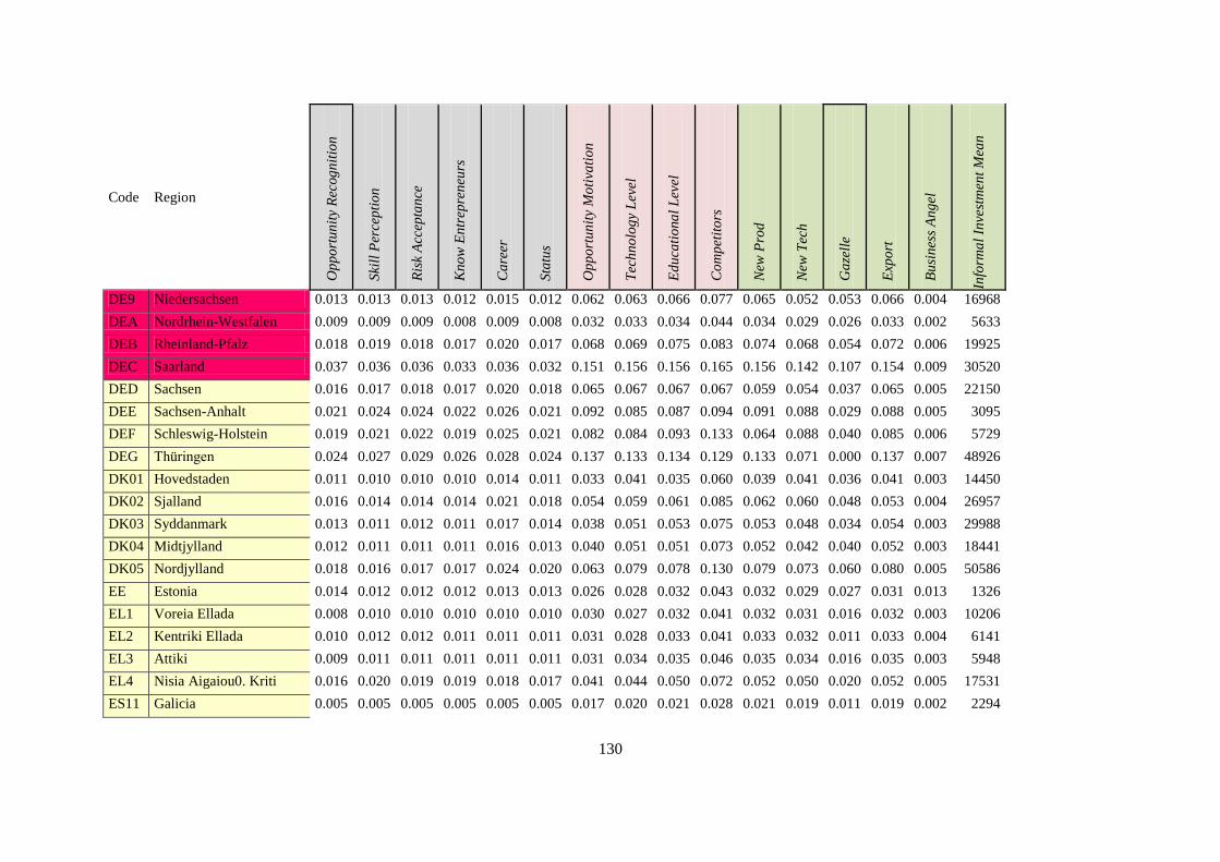
130
Code Region
Op
po
rtu
nit
y R
ecog
nit
ion
Ski
ll P
erce
pti
on
Ris
k A
ccep
tan
ce
Kn
ow
En
trep
ren
eurs
Ca
reer
Sta
tus
Op
po
rtu
nit
y M
oti
vati
on
Tec
hn
olo
gy
Lev
el
Ed
uca
tio
na
l L
evel
Co
mp
etit
ors
New
Pro
d
New
Tec
h
Ga
zell
e
Exp
ort
Bu
sin
ess
An
gel
Info
rma
l In
vest
men
t M
ean
DE9 Niedersachsen 0.013 0.013 0.013 0.012 0.015 0.012 0.062 0.063 0.066 0.077 0.065 0.052 0.053 0.066 0.004 16968
DEA Nordrhein-Westfalen 0.009 0.009 0.009 0.008 0.009 0.008 0.032 0.033 0.034 0.044 0.034 0.029 0.026 0.033 0.002 5633
DEB Rheinland-Pfalz 0.018 0.019 0.018 0.017 0.020 0.017 0.068 0.069 0.075 0.083 0.074 0.068 0.054 0.072 0.006 19925
DEC Saarland 0.037 0.036 0.036 0.033 0.036 0.032 0.151 0.156 0.156 0.165 0.156 0.142 0.107 0.154 0.009 30520
DED Sachsen 0.016 0.017 0.018 0.017 0.020 0.018 0.065 0.067 0.067 0.067 0.059 0.054 0.037 0.065 0.005 22150
DEE Sachsen-Anhalt 0.021 0.024 0.024 0.022 0.026 0.021 0.092 0.085 0.087 0.094 0.091 0.088 0.029 0.088 0.005 3095
DEF Schleswig-Holstein 0.019 0.021 0.022 0.019 0.025 0.021 0.082 0.084 0.093 0.133 0.064 0.088 0.040 0.085 0.006 5729
DEG Thüringen 0.024 0.027 0.029 0.026 0.028 0.024 0.137 0.133 0.134 0.129 0.133 0.071 0.000 0.137 0.007 48926
DK01 Hovedstaden 0.011 0.010 0.010 0.010 0.014 0.011 0.033 0.041 0.035 0.060 0.039 0.041 0.036 0.041 0.003 14450
DK02 Sjalland 0.016 0.014 0.014 0.014 0.021 0.018 0.054 0.059 0.061 0.085 0.062 0.060 0.048 0.053 0.004 26957
DK03 Syddanmark 0.013 0.011 0.012 0.011 0.017 0.014 0.038 0.051 0.053 0.075 0.053 0.048 0.034 0.054 0.003 29988
DK04 Midtjylland 0.012 0.011 0.011 0.011 0.016 0.013 0.040 0.051 0.051 0.073 0.052 0.042 0.040 0.052 0.003 18441
DK05 Nordjylland 0.018 0.016 0.017 0.017 0.024 0.020 0.063 0.079 0.078 0.130 0.079 0.073 0.060 0.080 0.005 50586
EE Estonia 0.014 0.012 0.012 0.012 0.013 0.013 0.026 0.028 0.032 0.043 0.032 0.029 0.027 0.031 0.013 1326
EL1 Voreia Ellada 0.008 0.010 0.010 0.010 0.010 0.010 0.030 0.027 0.032 0.041 0.032 0.031 0.016 0.032 0.003 10206
EL2 Kentriki Ellada 0.010 0.012 0.012 0.011 0.011 0.011 0.031 0.028 0.033 0.041 0.033 0.032 0.011 0.033 0.004 6141
EL3 Attiki 0.009 0.011 0.011 0.011 0.011 0.011 0.031 0.034 0.035 0.046 0.035 0.034 0.016 0.035 0.003 5948
EL4 Nisia Aigaiou0. Kriti 0.016 0.020 0.019 0.019 0.018 0.017 0.041 0.044 0.050 0.072 0.052 0.050 0.020 0.052 0.005 17531
ES11 Galicia 0.005 0.005 0.005 0.005 0.005 0.005 0.017 0.020 0.021 0.028 0.021 0.019 0.011 0.019 0.002 2294

131
Code Region
Op
po
rtu
nit
y R
ecog
nit
ion
Ski
ll P
erce
pti
on
Ris
k A
ccep
tan
ce
Kn
ow
En
trep
ren
eurs
Ca
reer
Sta
tus
Op
po
rtu
nit
y M
oti
vati
on
Tec
hn
olo
gy
Lev
el
Ed
uca
tio
na
l L
evel
Co
mp
etit
ors
New
Pro
d
New
Tec
h
Ga
zell
e
Exp
ort
Bu
sin
ess
An
gel
Info
rma
l In
vest
men
t M
ean
ES12 Principado de Asturias 0.005 0.006 0.006 0.005 0.006 0.006 0.024 0.026 0.028 0.035 0.028 0.028 0.015 0.027 0.002 4194
ES13 Cantabria 0.006 0.008 0.008 0.007 0.008 0.008 0.028 0.032 0.032 0.048 0.032 0.028 0.014 0.030 0.002 2353
ES21 País Vasco 0.005 0.005 0.005 0.005 0.005 0.005 0.019 0.022 0.023 0.032 0.023 0.021 0.011 0.021 0.002 5384
ES22 Comunidad Foral de
Navarra
0.005 0.006 0.006 0.005 0.005 0.006 0.020 0.021 0.023 0.033 0.023 0.021 0.011 0.021 0.002 4236
ES23 La Rioja 0.008 0.009 0.009 0.009 0.009 0.009 0.029 0.037 0.038 0.055 0.039 0.037 0.020 0.034 0.003 2874
ES24 Aragón 0.005 0.006 0.006 0.006 0.006 0.006 0.019 0.022 0.025 0.033 0.024 0.021 0.013 0.022 0.002 4673
ES30 Comunidad de Madrid 0.005 0.005 0.005 0.005 0.005 0.005 0.015 0.018 0.018 0.024 0.019 0.018 0.011 0.018 0.002 3747
ES41 Castilla y León 0.005 0.007 0.006 0.006 0.007 0.007 0.024 0.025 0.027 0.040 0.027 0.026 0.012 0.025 0.002 3153
ES42 Castilla-la Mancha 0.006 0.007 0.007 0.006 0.007 0.007 0.024 0.023 0.028 0.037 0.027 0.025 0.014 0.026 0.002 6277
ES43 Extremadura 0.006 0.007 0.007 0.007 0.007 0.008 0.026 0.029 0.031 0.042 0.030 0.026 0.012 0.028 0.002 1922
ES51 Cataluna 0.005 0.005 0.005 0.005 0.005 0.005 0.015 0.018 0.019 0.026 0.019 0.015 0.010 0.018 0.002 3850
ES52 Comunidad Valenciana 0.005 0.005 0.005 0.005 0.005 0.005 0.017 0.019 0.020 0.027 0.020 0.018 0.009 0.018 0.002 2058
ES53 Illes Balears 0.008 0.010 0.010 0.009 0.010 0.010 0.028 0.034 0.036 0.050 0.036 0.034 0.020 0.033 0.003 8476
ES61 Andalucía 0.005 0.006 0.006 0.005 0.006 0.006 0.020 0.021 0.022 0.032 0.021 0.020 0.011 0.020 0.002 3392
ES62 Región de Murcia 0.005 0.006 0.006 0.006 0.006 0.006 0.020 0.023 0.023 0.031 0.023 0.023 0.012 0.021 0.002 3621
ES70 Canarias (ES) 0.005 0.006 0.006 0.005 0.005 0.006 0.018 0.020 0.021 0.028 0.021 0.019 0.012 0.020 0.002 3448
FI19 Länsi-Suomi 0.012 0.010 0.010 0.010 0.010 0.008 0.028 0.037 0.034 0.041 0.034 0.031 0.025 0.032 0.003 3681
FI1B Helsinki-Uusimaa 0.016 0.013 0.012 0.013 0.013 0.009 0.041 0.050 0.046 0.055 0.046 0.041 0.024 0.045 0.004 9496
FI1C Etelä-Suomi 0.015 0.013 0.012 0.013 0.014 0.009 0.038 0.045 0.045 0.058 0.046 0.040 0.029 0.045 0.004 2344
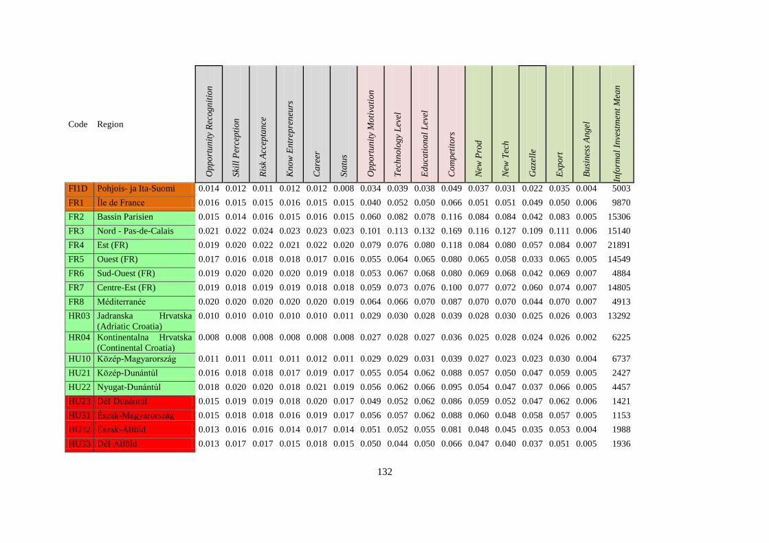
132
Code Region
Op
po
rtu
nit
y R
ecog
nit
ion
Ski
ll P
erce
pti
on
Ris
k A
ccep
tan
ce
Kn
ow
En
trep
ren
eurs
Ca
reer
Sta
tus
Op
po
rtu
nit
y M
oti
vati
on
Tec
hn
olo
gy
Lev
el
Ed
uca
tio
na
l L
evel
Co
mp
etit
ors
New
Pro
d
New
Tec
h
Ga
zell
e
Exp
ort
Bu
sin
ess
An
gel
Info
rma
l In
vest
men
t M
ean
FI1D Pohjois- ja Ita-Suomi 0.014 0.012 0.011 0.012 0.012 0.008 0.034 0.039 0.038 0.049 0.037 0.031 0.022 0.035 0.004 5003
FR1 Île de France 0.016 0.015 0.015 0.016 0.015 0.015 0.040 0.052 0.050 0.066 0.051 0.051 0.049 0.050 0.006 9870
FR2 Bassin Parisien 0.015 0.014 0.016 0.015 0.016 0.015 0.060 0.082 0.078 0.116 0.084 0.084 0.042 0.083 0.005 15306
FR3 Nord - Pas-de-Calais 0.021 0.022 0.024 0.023 0.023 0.023 0.101 0.113 0.132 0.169 0.116 0.127 0.109 0.111 0.006 15140
FR4 Est (FR) 0.019 0.020 0.022 0.021 0.022 0.020 0.079 0.076 0.080 0.118 0.084 0.080 0.057 0.084 0.007 21891
FR5 Ouest (FR) 0.017 0.016 0.018 0.018 0.017 0.016 0.055 0.064 0.065 0.080 0.065 0.058 0.033 0.065 0.005 14549
FR6 Sud-Ouest (FR) 0.019 0.020 0.020 0.020 0.019 0.018 0.053 0.067 0.068 0.080 0.069 0.068 0.042 0.069 0.007 4884
FR7 Centre-Est (FR) 0.019 0.018 0.019 0.019 0.018 0.018 0.059 0.073 0.076 0.100 0.077 0.072 0.060 0.074 0.007 14805
FR8 Méditerranée 0.020 0.020 0.020 0.020 0.020 0.019 0.064 0.066 0.070 0.087 0.070 0.070 0.044 0.070 0.007 4913
HR03 Jadranska Hrvatska
(Adriatic Croatia)
0.010 0.010 0.010 0.010 0.010 0.011 0.029 0.030 0.028 0.039 0.028 0.030 0.025 0.026 0.003 13292
HR04 Kontinentalna Hrvatska
(Continental Croatia)
0.008 0.008 0.008 0.008 0.008 0.008 0.027 0.028 0.027 0.036 0.025 0.028 0.024 0.026 0.002 6225
HU10 Közép-Magyarország 0.011 0.011 0.011 0.011 0.012 0.011 0.029 0.029 0.031 0.039 0.027 0.023 0.023 0.030 0.004 6737
HU21 Közép-Dunántúl 0.016 0.018 0.018 0.017 0.019 0.017 0.055 0.054 0.062 0.088 0.057 0.050 0.047 0.059 0.005 2427
HU22 Nyugat-Dunántúl 0.018 0.020 0.020 0.018 0.021 0.019 0.056 0.062 0.066 0.095 0.054 0.047 0.037 0.066 0.005 4457
HU23 Dél-Dunántúl 0.015 0.019 0.019 0.018 0.020 0.017 0.049 0.052 0.062 0.086 0.059 0.052 0.047 0.062 0.006 1421
HU31 Észak-Magyarország 0.015 0.018 0.018 0.016 0.019 0.017 0.056 0.057 0.062 0.088 0.060 0.048 0.058 0.057 0.005 1153
HU32 Észak-Alföld 0.013 0.016 0.016 0.014 0.017 0.014 0.051 0.052 0.055 0.081 0.048 0.045 0.035 0.053 0.004 1988
HU33 Dél-Alföld 0.013 0.017 0.017 0.015 0.018 0.015 0.050 0.044 0.050 0.066 0.047 0.040 0.037 0.051 0.005 1936

133
Code Region
Op
po
rtu
nit
y R
ecog
nit
ion
Ski
ll P
erce
pti
on
Ris
k A
ccep
tan
ce
Kn
ow
En
trep
ren
eurs
Ca
reer
Sta
tus
Op
po
rtu
nit
y M
oti
vati
on
Tec
hn
olo
gy
Lev
el
Ed
uca
tio
na
l L
evel
Co
mp
etit
ors
New
Pro
d
New
Tec
h
Ga
zell
e
Exp
ort
Bu
sin
ess
An
gel
Info
rma
l In
vest
men
t M
ean
IE01 Border0. Midland and
Western
0.013 0.015 0.014 0.014 0.015 0.011 0.045 0.047 0.042 0.066 0.048 0.043 0.036 0.047 0.005 13305
IE02 Southern and Eastern 0.008 0.008 0.008 0.008 0.008 0.006 0.024 0.026 0.024 0.038 0.027 0.024 0.023 0.027 0.003 8214
ITC Nord-Ovest 0.012 0.012 0.012 0.010 0.012 0.012 0.039 0.050 0.048 0.058 0.048 0.044 0.036 0.050 0.003 19944
ITF Sud 0.012 0.012 0.012 0.012 0.012 0.012 0.045 0.050 0.049 0.062 0.049 0.049 0.028 0.047 0.003 7408
ITG Isole 0.017 0.018 0.018 0.017 0.017 0.017 0.056 0.063 0.067 0.074 0.067 0.065 0.037 0.066 0.004 26221
ITH Nord-Est 0.014 0.013 0.014 0.013 0.014 0.014 0.044 0.058 0.059 0.079 0.058 0.053 0.025 0.054 0.003 18207
ITI Centro (IT) 0.013 0.014 0.014 0.012 0.014 0.014 0.048 0.058 0.058 0.069 0.060 0.059 0.036 0.060 0.003 7786
LT Lithuania 0.010 0.011 0.011 0.010 . . 0.030 0.026 0.027 0.047 0.032 0.032 0.030 0.032 0.005 5636
LV Latvia 0.006 0.006 0.006 0.006 0.007 0.007 0.015 0.017 0.017 0.022 0.017 0.015 0.015 0.017 0.002 2922
NL1 Noord-Nederland 0.017 0.016 0.015 0.015 0.012 0.016 0.039 0.050 0.049 0.080 0.056 0.044 0.032 0.056 0.004 21016
NL2 Oost-Nederland 0.013 0.011 0.010 0.011 0.009 0.011 0.034 0.039 0.036 0.061 0.041 0.035 0.027 0.040 0.003 10921
NL3 West-Nederland 0.009 0.008 0.007 0.008 0.006 0.008 0.019 0.024 0.024 0.033 0.024 0.020 0.017 0.025 0.002 10771
NL4 Zuid-Nederland 0.013 0.012 0.011 0.011 0.009 0.011 0.034 0.038 0.038 0.054 0.038 0.031 0.024 0.039 0.003 20481
PL1 Region Centralny 0.017 0.018 0.017 0.017 0.016 0.018 0.062 0.035 0.061 0.068 0.056 0.056 0.050 0.049 0.006 1212
PL2 Region Poludniowy 0.018 0.018 0.018 0.017 0.017 0.018 0.057 0.043 0.052 0.074 0.051 0.041 0.047 0.048 0.007 10090
PL3 Region Wschodni 0.017 0.019 0.018 0.018 0.017 0.019 0.064 0.040 0.056 0.081 0.053 0.059 0.057 0.061 0.006 2593
PL4 Region Pólnocno-
Zachodni
0.018 0.020 0.020 0.019 0.019 0.020 0.063 0.043 0.056 0.096 0.060 0.059 0.055 0.056 0.007 24837
PL5 Region Poludniowo-
Zachodni
0.024 0.025 0.025 0.024 0.024 0.025 0.071 0.059 0.077 0.113 0.064 0.070 0.066 0.070 0.017 22460
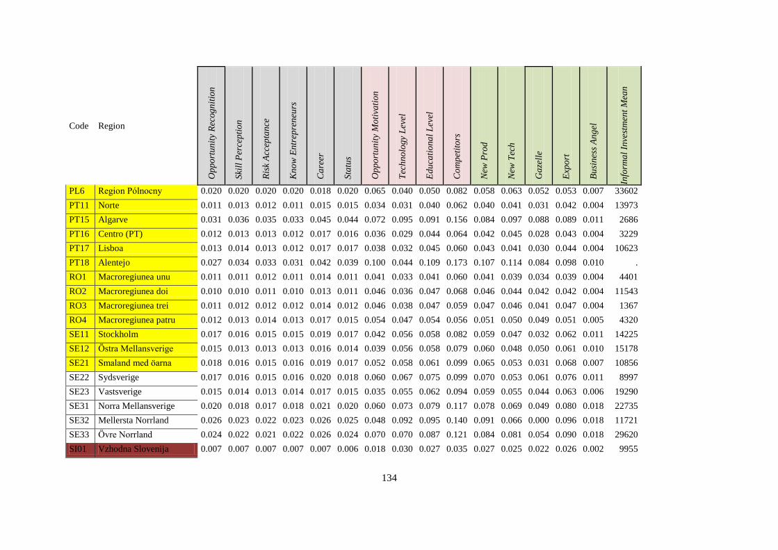
134
Code Region
Op
po
rtu
nit
y R
ecog
nit
ion
Ski
ll P
erce
pti
on
Ris
k A
ccep
tan
ce
Kn
ow
En
trep
ren
eurs
Ca
reer
Sta
tus
Op
po
rtu
nit
y M
oti
vati
on
Tec
hn
olo
gy
Lev
el
Ed
uca
tio
na
l L
evel
Co
mp
etit
ors
New
Pro
d
New
Tec
h
Ga
zell
e
Exp
ort
Bu
sin
ess
An
gel
Info
rma
l In
vest
men
t M
ean
PL6 Region Pólnocny 0.020 0.020 0.020 0.020 0.018 0.020 0.065 0.040 0.050 0.082 0.058 0.063 0.052 0.053 0.007 33602
PT11 Norte 0.011 0.013 0.012 0.011 0.015 0.015 0.034 0.031 0.040 0.062 0.040 0.041 0.031 0.042 0.004 13973
PT15 Algarve 0.031 0.036 0.035 0.033 0.045 0.044 0.072 0.095 0.091 0.156 0.084 0.097 0.088 0.089 0.011 2686
PT16 Centro (PT) 0.012 0.013 0.013 0.012 0.017 0.016 0.036 0.029 0.044 0.064 0.042 0.045 0.028 0.043 0.004 3229
PT17 Lisboa 0.013 0.014 0.013 0.012 0.017 0.017 0.038 0.032 0.045 0.060 0.043 0.041 0.030 0.044 0.004 10623
PT18 Alentejo 0.027 0.034 0.033 0.031 0.042 0.039 0.100 0.044 0.109 0.173 0.107 0.114 0.084 0.098 0.010 .
RO1 Macroregiunea unu 0.011 0.011 0.012 0.011 0.014 0.011 0.041 0.033 0.041 0.060 0.041 0.039 0.034 0.039 0.004 4401
RO2 Macroregiunea doi 0.010 0.010 0.011 0.010 0.013 0.011 0.046 0.036 0.047 0.068 0.046 0.044 0.042 0.042 0.004 11543
RO3 Macroregiunea trei 0.011 0.012 0.012 0.012 0.014 0.012 0.046 0.038 0.047 0.059 0.047 0.046 0.041 0.047 0.004 1367
RO4 Macroregiunea patru 0.012 0.013 0.014 0.013 0.017 0.015 0.054 0.047 0.054 0.056 0.051 0.050 0.049 0.051 0.005 4320
SE11 Stockholm 0.017 0.016 0.015 0.015 0.019 0.017 0.042 0.056 0.058 0.082 0.059 0.047 0.032 0.062 0.011 14225
SE12 Östra Mellansverige 0.015 0.013 0.013 0.013 0.016 0.014 0.039 0.056 0.058 0.079 0.060 0.048 0.050 0.061 0.010 15178
SE21 Smaland med öarna 0.018 0.016 0.015 0.016 0.019 0.017 0.052 0.058 0.061 0.099 0.065 0.053 0.031 0.068 0.007 10856
SE22 Sydsverige 0.017 0.016 0.015 0.016 0.020 0.018 0.060 0.067 0.075 0.099 0.070 0.053 0.061 0.076 0.011 8997
SE23 Vastsverige 0.015 0.014 0.013 0.014 0.017 0.015 0.035 0.055 0.062 0.094 0.059 0.055 0.044 0.063 0.006 19290
SE31 Norra Mellansverige 0.020 0.018 0.017 0.018 0.021 0.020 0.060 0.073 0.079 0.117 0.078 0.069 0.049 0.080 0.018 22735
SE32 Mellersta Norrland 0.026 0.023 0.022 0.023 0.026 0.025 0.048 0.092 0.095 0.140 0.091 0.066 0.000 0.096 0.018 11721
SE33 Övre Norrland 0.024 0.022 0.021 0.022 0.026 0.024 0.070 0.070 0.087 0.121 0.084 0.081 0.054 0.090 0.018 29620
SI01 Vzhodna Slovenija 0.007 0.007 0.007 0.007 0.007 0.006 0.018 0.030 0.027 0.035 0.027 0.025 0.022 0.026 0.002 9955

135
Code Region
Op
po
rtu
nit
y R
ecog
nit
ion
Ski
ll P
erce
pti
on
Ris
k A
ccep
tan
ce
Kn
ow
En
trep
ren
eurs
Ca
reer
Sta
tus
Op
po
rtu
nit
y M
oti
vati
on
Tec
hn
olo
gy
Lev
el
Ed
uca
tio
na
l L
evel
Co
mp
etit
ors
New
Pro
d
New
Tec
h
Ga
zell
e
Exp
ort
Bu
sin
ess
An
gel
Info
rma
l In
vest
men
t M
ean
SI02 Zahodna Slovenija 0.008 0.008 0.007 0.008 0.008 0.007 0.019 0.030 0.026 0.035 0.026 0.024 0.020 0.025 0.002 5903
SK01 Bratislavsky kraj 0.024 0.023 0.022 0.023 0.023 0.022 0.047 0.050 0.056 0.090 0.058 0.058 0.052 0.052 0.013 19148
SK02 Západné Slovensko 0.012 0.014 0.013 0.013 0.014 0.013 0.036 0.034 0.034 0.047 0.039 0.038 0.028 0.039 0.011 15839
SK03 Stredné Slovensko 0.013 0.016 0.016 0.016 0.016 0.015 0.042 0.035 0.040 0.053 0.044 0.043 0.037 0.041 0.008 12805
SK04 Vychodné Slovensko 0.012 0.015 0.015 0.015 0.016 0.014 0.044 0.033 0.038 0.056 0.045 0.044 0.036 0.045 0.011 15918
UKC North East (UK) 0.009 0.009 0.009 0.008 0.009 0.008 0.025 0.028 0.029 0.039 0.029 0.024 0.020 0.027 0.001 13506
UKD North West (UK) 0.009 0.009 0.008 0.007 0.009 0.008 0.024 0.027 0.027 0.038 0.027 0.024 0.021 0.027 0.001 6177
UKE Yorkshire and The
Humber
0.007 0.007 0.007 0.006 0.007 0.006 0.019 0.023 0.023 0.031 0.022 0.020 0.018 0.022 0.001 10299
UKF East Midlands (UK) 0.009 0.009 0.009 0.008 0.009 0.008 0.025 0.028 0.028 0.037 0.027 0.025 0.019 0.028 0.002 18373
UKG West Midlands (UK) 0.008 0.008 0.008 0.007 0.009 0.007 0.021 0.025 0.025 0.034 0.025 0.022 0.019 0.025 0.002 10018
UKH East of England 0.014 0.014 0.013 0.012 0.014 0.013 0.031 0.037 0.037 0.051 0.038 0.037 0.026 0.038 0.002 11782
UKI London 0.010 0.010 0.009 0.009 0.010 0.009 0.024 0.027 0.027 0.035 0.027 0.026 0.023 0.026 0.002 12699
UKJ South East (UK) 0.009 0.008 0.008 0.007 0.009 0.008 0.021 0.027 0.026 0.035 0.025 0.022 0.020 0.027 0.001 16071
UKK South West (UK) 0.010 0.010 0.010 0.009 0.011 0.009 0.025 0.029 0.030 0.040 0.030 0.027 0.021 0.030 0.002 12647
UKL Wales 0.006 0.007 0.006 0.006 0.007 0.006 0.017 0.019 0.020 0.028 0.020 0.017 0.016 0.020 0.001 8757
UKM Scotland 0.010 0.010 0.010 0.009 0.011 0.009 0.028 0.036 0.036 0.051 0.035 0.031 0.026 0.036 0.001 12588
UKN Northern Ireland (UK) 0.008 0.008 0.008 0.007 0.009 0.007 0.024 0.027 0.028 0.036 0.028 0.024 0.023 0.028 0.002 7667

136
7.3 Appendix C: The description and source of the institutional variables and indicators used in the
REDI
Institutional
variable
Description Source
of data
Data availability
(Available: August 8, 2013)
Market
Agglomeration
1) POPULATION GROWTH: Population on 1 January by age and sex - NUTS 2 regions, 2005-2012: The inhabitants of a
given area on 1 January of the year in question (or, in some cases, on 31 December of the previous year). The population
is based on data from the most recent census adjusted by the components of population change produced since the last census, or based on population registers. (regional level).
2) URBANIZATION: World Urbanization Prospects: The 2011 Revision, Population of Urban and Rural Areas and Percentage Urban, 2011 (country level); Cluster Observatory Degree of urbanization data (2010–2011) (regional level)
3) ACCESSIBILITY : Gravity model used to determine the sphere of influence of each central location by estimating where
the breaking point between the two settlements (here regions) will be (regional level). Using regional gross domestic product (GDP) by NUTS 2 regions (million EUR, 2010) data and total land area by NUTS 2 region (km2, 2010) (regional
level)10
GDP (gross domestic product) is an indicator of the output of a country or a region. It reflects the total value of all goods and services produced less the value of goods and services used for intermediate consumption in their
production. Expressing GDP in PPS (purchasing power standards) eliminates differences in price levels between countries. Calculations on a per inhabitant basis allow for the comparison of economies and regions significantly
different in absolute size. GDP per inhabitant in PPS is a key variable for determining the eligibility of NUTS 2
regions in the framework of the European Union’s structural policy.
Total land area by NUTS 2 regions (km2): For calculation of population density, the land area (excluding inland
water bodies like lakes or rivers) should be used when available. In several countries the total area, including area of lakes and rivers, is used because it is the only aspect for which data are available.
Calculation: simple average of the indicators of Population Growth, Urbanization and Accessibility variables.
Box-cox transformation11 was used in the case of the Accessibility variable, because the skewness of the original variable was higher than 1 (original value: 5.459). Therefore λ = -0.05.
Eurostat Regional Database
United Nations, Department of Economic and Social Affairs,
Population Division Cluster Observatory (Regional
Indicators – Degree of
Urbanization)
http://epp.eurostat.ec.europa.eu/t
gm/table.do?tab=table&init=1&l
anguage=en&pcode=tgs00096&plugin=1
http://esa.un.org/unpd/wup/CD-
ROM/Urban-Rural-Population.htm
http://www.clusterobservatory.eu
/index.html#!view=regionalmapping;i=C22300;y=2011;r=NC10;
rsl=2;rp=NC10;sp=CC20-STND;p=table
http://epp.eurostat.ec.europa.eu/t
gm/table.do?tab=table&init=1&language=en&pcode=tgs00003&
plugin=1
http://epp.eurostat.ec.europa.eu/tgm/table.do?tab=table&init=1&l
anguage=en&pcode=tgs00002&
plugin=1
10
Gravity model is characterized by an indicator which measures the market potential of the different locations. The extent of the gravity depends on the mass of the two locations (that can be measured by population,
GDP and so on) and on the distance between locations. The formula of the indicator is
where i is index of the region, and j is the index of the other region. M is the indicator of the mass (here it is the GDP on PPS on a unit of area measured with square kilometer), and dij is the distance between the ith and the jth regions (here measured with calculated the Eucladean distance of the centroids of the given NUTS1 or NUTS2 regions).
GDP data originates from the Eurostat regional database. 11
EU Regional Competitiveness Index, 2010 (Data transformation), page 52-53.

137
Quality of
Education
1) PISA (country level)
- Low achievers in Reading of 15-year-olds, 2006. - Low achievers in Math of 15-year-olds, 2006.
- Low achievers in Science of 15-year-olds, 2006.
2) CREATIVE CLASS (SCIENTIFIC TALENT) (regional level) - Annual employment in creative class / economically active population, 2008.
- Number of jobs in the creative workforce per active population, 2008.
Calculation: after subtracting from 100 the average of the three PISA variables, the average value was multiplied with the
simple average of the two indicators of Creative Class (Scientific Talent). Box-cox transformation was used in the case of
the average PISA variable, because the skewness of the original variable was higher than -1 (-2.119). Therefore λ =2. Also a second transformation was necessary to handle the skewness of the variable (again λ =2).
OECD – PISA database
ESPON Database Portal (Theme: Information and Society –
Employment in Creative Class)
ESPON Database Portal (Project: CREA Update – Creative
Workforce Update – Share of the
creative workforce) ESPON Database Portal (Theme:
Economy, finance and trade –
Economically active population)
http://pisacountry.acer.edu.au/
http://database.espon.eu/db2/sear
ch;jsessionid=db8d55d87de9e3a650e2a3b1f293
Business Risk
BUSINESS EXTENT OF DISCLOSURE INDEX (country level)
Disclosure index measures the extent to which investors are protected through disclosure of ownership and financial information. The index ranges from 0 to 10, with higher values indicating greater disclosure, (0=least disclosure to
10=greatest disclosure), for year 2012.
The indicators distinguish three dimensions of investor protections: transparency of related-party transactions (extent of disclosure index), liability for self-dealing (extent of director liability index) and shareholders’ ability to sue officers and
directors for misconduct (ease of shareholder suits index). The data come from a survey of corporate and securities lawyers
and are based on securities regulations, company laws, civil procedure codes and court rules of evidence. Detailed description is available at: http://www.doingbusiness.org/methodology/protecting-investors (5 August 2013).
World Bank
World Development Index
http://data.worldbank.org/indicat
or/IC.BUS.DISC.XQ
Social Capital
1) SOCIAL CAPITAL (country level)
The sub-index measures countries’ performance in two areas: social cohesion and engagement; and community and family
networks. This sub-index evaluates how factors such as volunteering, helping strangers, and donating to charitable organisations impact economic performance and life satisfaction. It also measures levels of trust, whether citizens believe
they can rely on others, and assesses how marriage and religious attendance provide support networks beneficial to wellbeing. Empirical studies on social capital have shown that citizens’ wellbeing improves through social trust, family and
community ties, and civic group membership. Similarly, societies with lower levels of social capital have been shown to
experience lower levels of economic growth. And so the term ‘capital’ in ‘social capital’ highlights the contribution of social networks as an asset that produces economic and wellbeing returns (for year 2011).
The Social Capital sub-index contains 7 sub-indicators: (1) Donations, (2) Helping Strangers, (3) Formal Volunteering, (4)
Marriage, (5) Perception of Social Support, (6) Religious Attendance, (7) Trust in Others. Data are available from 2011. Detailed description of the variable is available at: http://webapi.prosperity.com/download/pdf/PI2012_MethodologyV4.pdf
(5 August 2013)
2) TECHNOLOGICAL READINESS (regional level) - Households with access to broadband, 2011.
- Individuals who ordered goods or services over the Internet for private use, 2011.
- Households with access to Internet, 2011.
Calculation: re-scaled (converted to a scale of 0 to 10) Social Capital data were multiplied with the simple average of the
three indicators of Technological Readiness.
LEGATUM Prosperity Index,
Social Capital
Eurostat Regional Database
http://www.prosperity.com/Expl
oreData.aspx http://appsso.eurostat.ec.europa.e
u/nui/show.do?dataset=isoc_r_ia
cc_h&lang=en http://appsso.eurostat.ec.europa.e
u/nui/show.do?dataset=isoc_r_bl
t12_i&lang=en http://appsso.eurostat.ec.europa.e
u/nui/show.do?dataset=isoc_r_br
oad_h&lang=en
Open Society
1) PERSONAL FREEDOM (country level) The Personal Freedom sub-index measures countries’ performance in two areas: individual freedom and social tolerance.
The Personal Freedom sub-index captures the effects of freedom of choice, expression, movement, and belief, on a country’s
per capita GDP and the subjective wellbeing of its citizens. It also assesses how levels of tolerance of ethnic minorities and immigrants impact countries’ economic growth and citizens’ life satisfaction. Societies that foster strong civil rights and
Charron et al.(2011)
EU QoG Corruption Index (EQI) LEGATUM Prosperity Index,
Personal Freedom
http://www.qog.pol.gu.se/data/da
tadownloads/qogeuregionaldata/
http://www.prosperity.com/ExploreData.aspx

138
freedoms have been shown to enjoy increases in levels of satisfaction among their citizens. When citizens’ personal liberties
are protected, a country benefits from higher levels of national income (for year 2011). The Personal Freedom sub-index contains 5 sub-indicators: (1) Civil Liberties, (2) Civil Liberty and Free Choice, (3)
Satisfaction with Freedom of Choice, (4) Tolerance of Immigrants, (5) Tolerance of Minorities.
Detailed description of the variable is available at: http://webapi.prosperity.com/download/pdf/PI2012_MethodologyV4.pdf (5 August 2013)
2) CORRUPTION (regional level)
Data based on a standardized variable combining education (EdCor: region's aggregated score from survey question on the extent to which corruption persists in the education system in the region/area), health (HelCor: region's aggregated score
from survey question on the extent to which corruption persists in the health care system in the region/area, and general
public corruption (OtherCor: egion's aggregated score from survey question on the extent to which respondents felt other
citizens in the region/area use bribery to obtain public services) in addition to law enforcement (LawCor: region's aggregated
score from survey question on the extent to which corruption persists in the law enforcement in the region/area) and the
payment of bribes (HelBribe: region's aggregated score from survey question asking whether the respondents were forced to pay a bribe in the last 12 months to obtain any health care in the region/area. . Data are from 2009-2010.
[Source: Nicholas Charron , Lewis Dijkstra & Victor Lapuente (2013): Regional Governance Matters: Quality of
Government within European Union Member States, Regional Studies, DOI:10.1080/00343404.2013.770141 To link to this article: http://www.qog.pol.gu.se/digitalAssets/1446/1446579_regional-studies-article.pdf (9 August 2013)]
Detailed description of the variable is available at: http://www.qog.pol.gu.se/digitalAssets/1362/1362471_eqi---correlates-
codebook.pdf (9 August 2013) Calculation: re-scaled (converted to a scale of 0 to 10) Corruption data were multiplied with re-scaled (converted to a scale
of 0 to 10) Personal Freedom data.
Business
Environment
1) BUSINESS FREEDOM (country level)
Business freedom is a quantitative measure of the ability to start, operate, and close a business that represents the overall burden of regulation as well as the efficiency of government in the regulatory process. The business freedom score for each
country is a number between 0 and 100, with 100 equaling the most free business environment. The score is based on 10 factors, all weighted equally, using data from the World Bank’s Doing Business report. Each factor is converted to a scale of
0 to 100, after which the average of the converted values is computed. The result represents the country’s business freedom
score, 2013. Detailed description of the variable is available at: http://www.heritage.org/index/business-freedom (5 August 2013).
2) EU QoG INDEX (regional level)
Data shows quality of government. Data based on a study on regional variation in quality of government within the EU The dataset covers all 27 EU countries as well as 172 NUTS 1 and NUTS 2 regions within 18 of the 27 countries, thus the data is
given for 181 separate units. The data for region ns was collected via a large survey of roughly 34,000 respondents in Europe
in December of 2009. The national level estimates are taken from the World Bank Governance Indicators. The regional estimates are comprised of 16 separate indicators. Data are from 2009-2010.
[Source: Nicholas Charron , Lewis Dijkstra & Victor Lapuente (2013): Regional Governance Matters: Quality of
Government within European Union Member States, Regional Studies, DOI:10.1080/00343404.2013.770141 To link to this
article: http://www.qog.pol.gu.se/digitalAssets/1446/1446579_regional-studies-article.pdf (9 August 2013)]
Detailed description of the variable is available at:
http://www.qog.pol.gu.se/data/datadownloads/qogeuregionaldata/ (5 August 2013). Calculation: Business Freedom indicator was multiplied with the re-scaled EU QoG index.
Heritage Foundation EU QoG Index
http://www.heritage.org/index/explore
http://ec.europa.eu/regional_poli
cy/sources/docgener/work/2012_02_governance.pdf
Absorptive
Capacity
1) FIRM-LEVEL TECHNOLOGY ABSORPTION (country level)
This data is taken from the WEF Global Competitiveness Report. Technological readiness is the 9th pillar of the Global
Competitiveness Index (GCI). The pillar contains two sub-indicators: (1) Technological adoption and (2) ICT use. In today’s globalized world, technology is increasingly essential for firms to compete and prosper. The Technological readiness pillar
measures the agility with which an economy adopts existing technologies to enhance the productivity of its industries, with
World Economic Forum
Competitiveness Report 2012-
2013, 489. p.
Eurostat Regional Database
http://www3.weforum.org/docs/
WEF_GlobalCompetitivenessRe
port_2012-13.pdf
http://epp.eurostat.ec.europa.eu/t

139
specific emphasis on its capacity to fully leverage information
and communication technologies (ICT) in daily activities and production processes for increased efficiency and enabling innovation for competitiveness. The variable of Firm-level technology absorption is a part of the Technological readiness
pillar. The variable answer the question to what extent do businesses in a country absorb new technology (1 = not at all; 7 =
aggressively absorb). Weighted average of 2011–12 data. Detailed description of the variable is available at: http://www3.weforum.org/docs/CSI/2012-13/GCR_Chapter1.1_2012-
13.pdf (9 August 2013)
2) EMPLOYMENT IN KNOWLEDGE INTENSIVE AND HIGH TECHNOLOGY ADOPTIONS (regional level)
• Employment in high-Technology Adoptions (high-tech manufacturing and knowledge-intensive services) by NUTS
2 region (2007-2008).
• Employment in technology and knowledge-intensive sectors by NUTS 2 region and gender (from 2008 onwards,
NACE Rev. 2) (2011)
• Researchers, all sectors by NUTS 2 region, % of total employment (2009). • Annual data on Human resources in science and technology (HRST) and sub-groups by NUTS 2 region (2011).
Calculation: Firm-level Technology Absorption variable was multiplied with the average of variables related to employment
in knowledge-intensive and high-Technology Adoptions.
gm/table.do?tab=table&init=1&l
anguage=en&pcode=tgs00039&
plugin=1
http://appsso.eurostat.ec.europa.e
u/nui/show.do?dataset=htec_emp
_reg2&lang=en
http://epp.eurostat.ec.europa.eu/t
gm/table.do?tab=table&init=1&l
anguage=en&pcode=tgs00043&
plugin=1
http://epp.eurostat.ec.europa.eu/t
gm/table.do?tab=table&init=1&l
anguage=en&pcode=tgs00038&
plugin=1
Education &
Training
HIGHER EDUCATION AND TRAINING AND LIFE-LONG LEARNING (regional level) - Share of population aged 25-64 years with higher educational attainment, 2011. [Source: Eurostat Regional
Database: Persons aged 25-64 with tertiary education attainment by sex and NUTS 2 regions (from 2000
onwards) - %] - Share of population aged 25-64 years participating in education and training, 2011. [Source: Eurostat Regional
Database: Participation of adults aged 25-64 in education and training by NUTS 2 regions (from 2000 onwards) -
%]
Calculation: The sum of the two variables is used.
Eurostat Regional Database
http://appsso.eurostat.ec.europa.e
u/nui/show.do?dataset=edat_lfse
_11&lang=en http://appsso.eurostat.ec.europa.e
u/nui/show.do?dataset=trng_lfse
_04&lang=en
Business
Strategy
1) NATURE OF COMPETITIVE ADVANTAGE (country level) This data is taken from the WEF Global Competitiveness Report. Business sophistication is the 11th pillar of the Global
Competitiveness Index (GCI). There is no doubt that sophisticated business practices are conducive to higher efficiency in
the production of goods and services. Business sophistication concerns two elements that are intricately linked: the quality of a country’s overall business networks and the quality of individual firms’ operations and strategies. These factors
are particularly important for countries at an advanced stage of development when, to a large extent, the more basic sources
of productivity improvements have been exhausted. The quality of a country’s business networks and supporting industries, as measured by the quantity and quality of local suppliers and the extent of their interaction, is important for a variety of
reasons. When companies and suppliers from a particular sector are interconnected in geographically proximate groups,
called clusters, efficiency is heightened, greater opportunities for innovation in processes and products are created, and barriers to entry for new firms are reduced. Individual firms’ advanced operations and strategies (branding, marketing,
distribution, advanced production processes, and the production of unique and sophisticated products) spill over into the
economy and lead to sophisticated and modern business processes across the country’s business sectors. The variable of Nature of competitive advantage is a part of the Technological readiness pillar. The data captures answers to the question:
“What is the nature of competitive advantage of your country’s companies in international markets based upon?” (1 = low-
cost or natural resources; 7 = unique products and processes). Weighted average of 2011–12 data. Detailed description of the variable is available at: http://www3.weforum.org/docs/CSI/2012-13/GCR_Chapter1.1_2012-
13.pdf (9 August 2013)
2) BUSINESS SOPHISTICATION (regional level)
- Share of employment in sophisticated sectors, 2011. [Employment in the J, K sectors as % of total employment,
World Economic Forum
Competitiveness Report 2012-
2013, 489. p. Eurostat Regional Database
(Total – All NACE activities, J –
Information and communication,
K – Financial and insurance
activities)
EU Regional Competitiveness Index, 2010
http://www3.weforum.org/docs/
WEF_GlobalCompetitivenessReport_2012-13.pdf
http://appsso.eurostat.ec.europa.e
u/nui/submitViewTableAction.do;jsessionid=9ea7d07d30e456f8
33bccf984d05b62de462168ef89f
.e34MbxeSaxaSc40LbNiMbxeNaNeKe0
http://appsso.eurostat.ec.europa.e
u/nui/submitViewTableAction.do
http://www.urenio.org/wp-
content/uploads/2010/09/Regional-Competitive-Index-EU-
JRC2010.pdf

140
J: Information and Communication, K: Financing and insurance activities.]
- Share of Gross value added (GVA) in sophisticated sectors, 2007. [GVA in the J, K sectors as % of total GVA, J: Information and Communication, K: Financing and insurance activities.]
- New foreign firms per one million inhabitants, 2005-2007.
Calculation: The Nature of competitive advantage was multiplied with the unweighted average of the three indicators of the
Business Sophistication variable. Box-cox transformation was used in the case of the ‘Employment in JK Sectors’ sub-
indicator, because the skewness of the original variables were higher than 1 (1.499). Therefore λ = -0.05.
Technology
Transfer
1) INNOVATION SUB-INDEX (same variables were used as in the EU Regional Competitiveness Index (2010), but data were updated) (regional level)
- Total patent applications: Patent applications to the EPO by priority year by NUTS 2 regions. Number of
applications per one million inhabitants (2008-2009 average). - Scientific publication: Publications per one million inhabitants (Thomson Reuters Web of Science & CWTS
database (Leiden University). Average of years 2005-2006.
- High-tech inventors: High-tech patent applications to the EPO by priority year by NUTS 2 regions. Number of applications per one million inhabitants (2008-2009 average).
- ICT inventors: PCT patent applications (fractional count by inventor and priority year) in ICT, 2010.
- Biotechnology inventors: PCT patent applications (fractional count by inventor and priority year) in biotech, 2010.
Calculation: unweighted average of the five innovation related variables. Box-cox transformation was used in the case of the indicator, because the skewness of the original indicator was higher than 1 (1.139). Therefore λ = -0.05
Eurostat Regional Database OECD Regional Database
(Innovation Indicators)
EU Regional Competitiveness Index, 2010
http://epp.eurostat.ec.europa.eu/tgm/table.do?tab=table&init=1&l
anguage=en&pcode=tgs00040&
plugin=1 http://epp.eurostat.ec.europa.eu/t
gm/table.do?tab=table&init=1&l
anguage=en&pcode=tgs00041&plugin=1
http://stats.oecd.org/Index.aspx?
datasetcode=REG_DEMO_TL2# http://www.urenio.org/wp-
content/uploads/2010/09/Region
al-Competitive-Index-EU-JRC2010.pdf
Technology
Development
GERD (regional level)
Gross Domestic Expenditure in Research & Development (GERD) as a percentage of GDP, for year 2009. (regional level)
Calculation: Box-cox transformation was used in the case of the GERD variable, because the skewness of the original
variable was higher than 1 (1.095). Therefore λ = -0.05.
Eurostat Regional Database
http://appsso.eurostat.ec.europa.e
u/nui/show.do?dataset=rd_e_ger
dreg&lang=en
Clustering
CLUSTERS (regional level) Cluster Mix Index
1. Average EU wage per cluster is calculated across the reporting countries, weighted by the total number of employees they
have in that cluster category at the national level. 2. Wages are normalized so that the cluster with the lowest average EU wage (that happened to be footwear) is equal to 1.
3. For each region, a wage cluster mix index is created by taking the sum across all clusters of the regional share in
employment per cluster times the relevant cluster wage index calculated above. This gives a number for each region; the higher it is the more the region benefits from the cluster mix effect rather than strong performance within any individual
cluster.
DGRegion Individual Datataset
(not-published)
Connectivity
INFRASTRUCTURE SUB-INDEX (regional level)
- Motorway density (average pop/area). EU27=100, Eurostat/DG TREN/EuroGeographics/National Statistical
Institutes, 2006.
- Railway density (average pop/area), EU27=100, Eurostat/DG TREN/EuroGeographics/National Statistical
Institutes, 2007. - Number of passenger flights, daily number of passenger flights (accessible within 90-minute drive),
Eurostat/EuroGeographics/National Statitical Institutes, 2007.
Calculation: Average of the variables of motorway density, railway density and number of passenger flights. Box-cox
transformation was used in the case of three transportation variables, because the skewness of the original variable was
higher than 1 (1.674). Therefore λ = -0.05.
EU Regional Competitiveness
Index, 2010
http://www.urenio.org/wp-
content/uploads/2010/09/Regional-Competitive-Index-EU-
JRC2010.pdf

141
Financial
Institutions
1) DEPTH OF CAPITAL MARKET (country level)
The Depth of Capital Market is one of the six sub-indices of the Venture Capital and Private Equity index. This variable is a complex measure of the size and liquidity of the stock market, level of IPO, M&A and debt and credit market activity. Note
that there were some methodological changes over the 2006-2012 time period so comparisons across years are not perfect.
The data set was provided by Alexander Groh, 2013. Detailed description about the indicator is available at: http://www.wall-street.ro/files/102434-82.pdf (5 August 2013).
2) CONCENTRATION OF FINANCIAL SERVICES (regional level) Regional employment in financial services sector as percentage of total regional employment (for different years between
2005-2011).
Calculation: Depth of Capital Market country level data were multiplied with the Concentration of Financial Services
variable. Box-cox transformation was used in the case of three transportation variables, because the skewness of the original
variable was higher than 1 (2.505). Therefore λ = -0.05.
Groh, A, H.Liechtenstein and K. Lieser 2012 The Global Venture
Capital and Private Equity
Country Attractiveness Index 2012 Annual,
Cluster Observatory (Financial services – employees, Regional
employment)
http://www.wall-street.ro/files/102434-82.pdf
http://www.clusterobservatory.eu
/index.html#!view=regionalmapping;i=V16140;y=2011;r=NC10;
rsl=2;rp=NC10;s=CC20-
fin;sp=CC20-STND;p=table http://www.clusterobservatory.eu
/index.html#!view=regionalmap
ping;i=V16140,C20220;y=2011;
r=NC10;rsl=2;rp=NC10;sp=CC2
0-STND;p=table
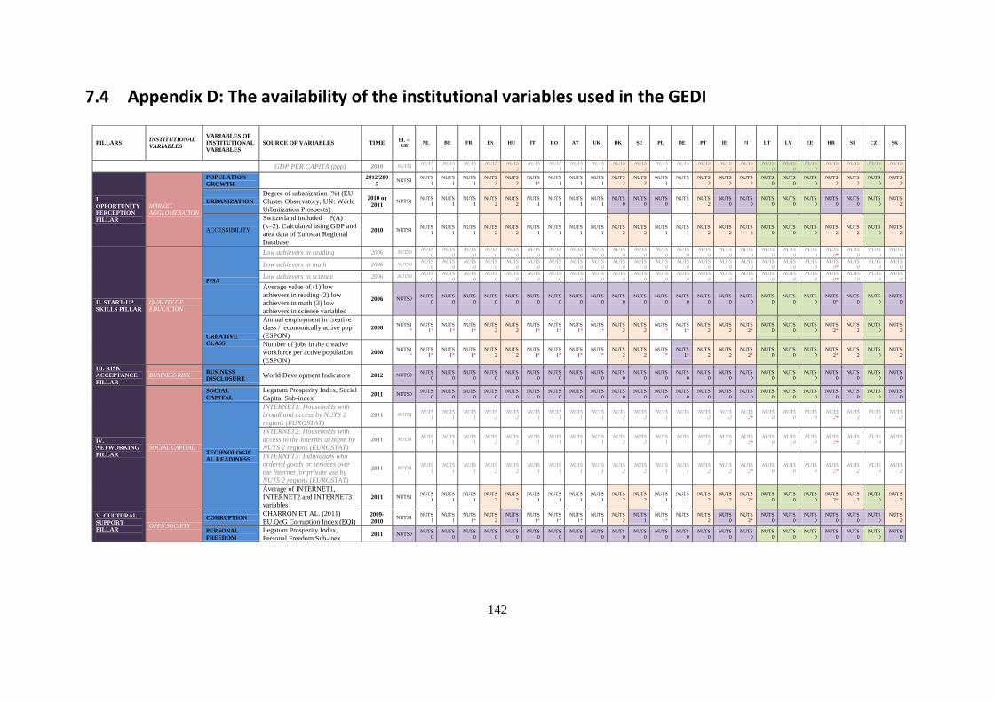
142
7.4 Appendix D: The availability of the institutional variables used in the GEDI
PILLARS INSTITUTIONAL
VARIABLES
VARIABLES OF
INSTITUTIONAL
VARIABLES
SOURCE OF VARIABLES TIME EL =
GR NL BE FR ES HU IT RO AT UK DK SE PL DE PT IE FI LT LV EE HR SI CZ SK
GDP PER CAPITA (ppp) 2010 NUTS1 NUTS
1
NUTS
1
NUTS
1
NUTS
2
NUTS
2
NUTS
1
NUTS
1
NUTS
1
NUTS
1
NUTS
2
NUTS
2
NUTS
1
NUTS
1
NUTS
2
NUTS
2
NUTS
2
NUTS
0
NUTS
0
NUTS
0
NUTS
2
NUTS
2
NUTS
0
NUTS
2
I.
OPPORTUNITY
PERCEPTION
PILLAR
MARKET
AGGLOMERATION
POPULATION
GROWTH
2012/200
5 NUTS1
NUTS
1
NUTS
1
NUTS
1
NUTS
2
NUTS
2
NUTS
1*
NUTS
1
NUTS
1
NUTS
1
NUTS
2
NUTS
2
NUTS
1
NUTS
1
NUTS
2
NUTS
2
NUTS
2
NUTS
0
NUTS
0
NUTS
0
NUTS
2
NUTS
2
NUTS
0
NUTS
2
URBANIZATION
Degree of urbanization (%) (EU
Cluster Observatory; UN: World
Urbanization Prospects)
2010 or
2011 NUTS1
NUTS
1
NUTS
1
NUTS
1
NUTS
2
NUTS
2
NUTS
1
NUTS
1
NUTS
1
NUTS
1
NUTS
0
NUTS
0
NUTS
0
NUTS
1
NUTS
2
NUTS
0
NUTS
0
NUTS
0
NUTS
0
NUTS
0
NUTS
0
NUTS
0
NUTS
0
NUTS
2
ACCESSIBILITY
Switzerland included P(A)
(k=2). Calculated using GDP and
area data of Eurostat Regional
Database
2010 NUTS1 NUTS
1
NUTS
1
NUTS
1
NUTS
2
NUTS
2
NUTS
1
NUTS
1
NUTS
1
NUTS
1
NUTS
2
NUTS
2
NUTS
1
NUTS
1
NUTS
2
NUTS
2
NUTS
2
NUTS
0
NUTS
0
NUTS
0
NUTS
2
NUTS
2
NUTS
0
NUTS
2
II. START-UP
SKILLS PILLAR
QUALITY OF
EDUCATION
PISA
Low achievers in reading 2006 NUTS0 NUTS
0 NUTS
0 NUTS
0 NUTS
0 NUTS
0 NUTS
0 NUTS
0 NUTS
0 NUTS
0 NUTS
0 NUTS
0 NUTS
0 NUTS
0 NUTS
0 NUTS
0 NUTS
0 NUTS
0 NUTS
0 NUTS
0 NUTS
0* NUTS
0 NUTS
0 NUTS
0
Low achievers in math 2006 NUTS0 NUTS
0 NUTS
0 NUTS
0 NUTS
0 NUTS
0 NUTS
0 NUTS
0 NUTS
0 NUTS
0 NUTS
0 NUTS
0 NUTS
0 NUTS
0 NUTS
0 NUTS
0 NUTS
0 NUTS
0 NUTS
0 NUTS
0 NUTS
0* NUTS
0 NUTS
0 NUTS
0
Low achievers in science 2006 NUTS0 NUTS
0 NUTS
0 NUTS
0 NUTS
0 NUTS
0 NUTS
0 NUTS
0 NUTS
0 NUTS
0 NUTS
0 NUTS
0 NUTS
0 NUTS
0 NUTS
0 NUTS
0 NUTS
0 NUTS
0 NUTS
0 NUTS
0 NUTS
0* NUTS
0 NUTS
0 NUTS
0
Average value of (1) low
achievers in reading (2) low
achievers in math (3) low
achievers in science variables
2006 NUTS0 NUTS
0
NUTS
0
NUTS
0
NUTS
0
NUTS
0
NUTS
0
NUTS
0
NUTS
0
NUTS
0
NUTS
0
NUTS
0
NUTS
0
NUTS
0
NUTS
0
NUTS
0
NUTS
0
NUTS
0
NUTS
0
NUTS
0
NUTS
0*
NUTS
0
NUTS
0
NUTS
0
CREATIVE
CLASS
Annual employment in creative
class / economically active pop
(ESPON)
2008 NUTS1
*
NUTS
1*
NUTS
1*
NUTS
1*
NUTS
2
NUTS
2
NUTS
1*
NUTS
1*
NUTS
1*
NUTS
1*
NUTS
2
NUTS
2
NUTS
1*
NUTS
1*
NUTS
2
NUTS
2
NUTS
2*
NUTS
0
NUTS
0
NUTS
0
NUTS
2*
NUTS
2
NUTS
0
NUTS
2
Number of jobs in the creative
workforce per active population
(ESPON)
2008 NUTS1
*
NUTS
1*
NUTS
1*
NUTS
1*
NUTS
2
NUTS
2
NUTS
1*
NUTS
1*
NUTS
1*
NUTS
1*
NUTS
2
NUTS
2
NUTS
1*
NUTS
1*
NUTS
2
NUTS
2
NUTS
2*
NUTS
0
NUTS
0
NUTS
0
NUTS
2*
NUTS
2
NUTS
0
NUTS
2
III. RISK
ACCEPTANCE
PILLAR
BUSINESS RISK BUSINESS
DISCLOSURE World Development Indicators 2012 NUTS0
NUTS
0
NUTS
0
NUTS
0
NUTS
0
NUTS
0
NUTS
0
NUTS
0
NUTS
0
NUTS
0
NUTS
0
NUTS
0
NUTS
0
NUTS
0
NUTS
0
NUTS
0
NUTS
0
NUTS
0
NUTS
0
NUTS
0
NUTS
0
NUTS
0
NUTS
0
NUTS
0
IV.
NETWORKING
PILLAR
SOCIAL CAPITAL
SOCIAL
CAPITAL
Legatum Prosperity Index, Social
Capital Sub-index 2011 NUTS0
NUTS
0
NUTS
0
NUTS
0
NUTS
0
NUTS
0
NUTS
0
NUTS
0
NUTS
0
NUTS
0
NUTS
0
NUTS
0
NUTS
0
NUTS
0
NUTS
0
NUTS
0
NUTS
0
NUTS
0
NUTS
0
NUTS
0
NUTS
0
NUTS
0
NUTS
0
NUTS
0
TECHNOLOGIC
AL READINESS
INTERNET1: Households with
broadband access by NUTS 2
regions (EUROSTAT)
2011 NUTS1 NUTS
1
NUTS
1
NUTS
1
NUTS
2
NUTS
2
NUTS
1
NUTS
1
NUTS
1
NUTS
1
NUTS
2
NUTS
2
NUTS
1
NUTS
1
NUTS
2
NUTS
2
NUTS
2*
NUTS
0
NUTS
0
NUTS
0
NUTS
2*
NUTS
2
NUTS
0
NUTS
2
INTERNET2: Households with
access to the Internet at home by
NUTS 2 regions (EUROSTAT)
2011 NUTS1 NUTS
1
NUTS
1
NUTS
1
NUTS
2
NUTS
2
NUTS
1
NUTS
1
NUTS
1
NUTS
1
NUTS
2
NUTS
2
NUTS
1
NUTS
1
NUTS
2
NUTS
2
NUTS
2*
NUTS
0
NUTS
0
NUTS
0
NUTS
2*
NUTS
2
NUTS
0
NUTS
2
INTERNET3: Individuals who
ordered goods or services over
the Internet for private use by
NUTS 2 regions (EUROSTAT)
2011 NUTS1 NUTS
1
NUTS
1
NUTS
1
NUTS
2
NUTS
2
NUTS
1
NUTS
1
NUTS
1
NUTS
1
NUTS
2
NUTS
2
NUTS
1
NUTS
1
NUTS
2
NUTS
2
NUTS
2*
NUTS
0
NUTS
0
NUTS
0
NUTS
2*
NUTS
2
NUTS
0
NUTS
2
Average of INTERNET1,
INTERNET2 and INTERNET3
variables
2011 NUTS1 NUTS
1
NUTS
1
NUTS
1
NUTS
2
NUTS
2
NUTS
1
NUTS
1
NUTS
1
NUTS
1
NUTS
2
NUTS
2
NUTS
1
NUTS
1
NUTS
2
NUTS
2
NUTS
2*
NUTS
0
NUTS
0
NUTS
0
NUTS
2*
NUTS
2
NUTS
0
NUTS
2
V. CULTURAL
SUPPORT
PILLAR
OPEN SOCIETY
CORRUPTION CHARRON ET AL. (2011)
EU QoG Corruption Index (EQI) 2009-
2010 NUTS1
NUTS
1
NUTS
1
NUTS
1*
NUTS
2
NUTS
1
NUTS
1*
NUTS
1*
NUTS
1*
NUTS
1
NUTS
2
NUTS
1
NUTS
1*
NUTS
1
NUTS
2
NUTS
0
NUTS
2*
NUTS
0
NUTS
0
NUTS
0
NUTS
0
NUTS
0
NUTS
0
NUTS
2
PERSONAL
FREEDOM
Legatum Prosperity Index,
Personal Freedom Sub-inex 2011 NUTS0
NUTS
0
NUTS
0
NUTS
0
NUTS
0
NUTS
0
NUTS
0
NUTS
0
NUTS
0
NUTS
0
NUTS
0
NUTS
0
NUTS
0
NUTS
0
NUTS
0
NUTS
0
NUTS
0
NUTS
0
NUTS
0
NUTS
0
NUTS
0
NUTS
0
NUTS
0
NUTS
0

143
PILLARS INSTITUTIONAL
VARIABLES
VARIABLES OF
INSTITUTIONAL
VARIABLES
SOURCE OF VARIABLES TIME EL =
GR NL BE FR ES HU IT RO AT UK DK SE PL DE PT IE FI LT LV EE HR SI CZ SK
VI. OPPORTUNITY
STARTUP PILLAR
BUSINESS
ENVIRONMENT
BUSINESS
FREEDOM Heritage Foundation 2013
NUTS0
NUTS0
NUTS0
NUTS0
NUTS0
NUTS0
NUTS0
NUTS0
NUTS0
NUTS0
NUTS0
NUTS0
NUTS0
NUTS0
NUTS0
NUTS0
NUTS0
NUTS0
NUTS0
NUTS0
NUTS0
NUTS0
NUTS0
NUTS0
EU QoG INDEX
Data shows quality of government. Data
based on A Study on Regional Variation in Quality of Government within the
EU. Charron et al. 2011.
2009-2010
NUTS
1
NUTS
1
NUTS
1
NUTS
1
NUTS
2
NUTS
2
NUTS
1
NUTS
1
NUTS
1
NUTS
1
NUTS
2
NUTS
2
NUTS
1
NUTS
1
NUTS
2
NUTS
2
NUTS
2*
NUTS
0
NUTS
0
NUTS
0
NUTS
2
NUTS
2
NUTS
0
NUTS
2
VII.
TECHNOLOGY
SECTOR PILLAR
ABSORPTIVE
CAPACITY
FIRM-LEVEL
TECHNOLOGY
ABSORPTION
The Global Competitiveness Index
2012-2013, World Economic Forum
2011–12
weighted
average NUTS
0
NUTS
0
NUTS
0
NUTS
0
NUTS
0
NUTS
0
NUTS
0
NUTS
0
NUTS
0
NUTS
0
NUTS
0
NUTS
0
NUTS
0
NUTS
0
NUTS
0
NUTS
0
NUTS
0
NUTS
0
NUTS
0
NUTS
0
NUTS
0
NUTS
0
NUTS
0
NUTS
0
EMPLOYMENT
IN KNOWLEDGE-
INTENSIVE AND
HIGH-
TECHNOLOGY
ADOPTIONS
Employment in high-Technology
Adoptions (high-tech manufacturing and
high-tech knowledge-intensive services) by NUTS 2 level
2008
NUTS
1
NUTS
1
NUTS
1
NUTS
1
NUTS
2
NUTS
2
NUTS
1
NUTS
1
NUTS
1
NUTS
1
NUTS
2
NUTS
2
NUTS
1
NUTS
1*
NUTS
2*
NUTS
2
NUTS
2
NUTS
0
NUTS
0
NUTS
0
NUTS
2
NUTS
2
NUTS
0
NUTS
2
Employment in technology and
knowledge-intensive sectors by NUTS 2 regions and sex
2011 NUTS
1
NUTS
1
NUTS
1
NUTS
1
NUTS
2*
NUTS
2
NUTS
1
NUTS
1
NUTS
1
NUTS
1
NUTS
2
NUTS
2
NUTS
1
NUTS
1*
NUTS
2*
NUTS
2
NUTS
2
NUTS
0
NUTS
0
NUTS
0
NUTS
2
NUTS
2
NUTS
0
NUTS
2
Researchers, all sectors by NUTS 2
regions % of total employment 2009
NUTS
1
NUTS
1
NUTS
2
NUTS
2
NUTS
1
NUTS
1
NUTS
1
NUTS
1
NUTS
2
NUTS
2
NUTS
1
NUTS
1
NUTS
2
NUTS
2
NUTS
2
NUTS
0
NUTS
0
NUTS
0
NUTS
2
NUTS
2
NUTS
0
NUTS
2
Annual data on HRST and sub-groups
by NUTS 2 regions 2011 NUTS
1 NUTS1
NUTS1
NUTS1
NUTS2
NUTS2
NUTS1
NUTS1
NUTS1
NUTS1
NUTS2
NUTS2
NUTS1
NUTS1
NUTS2
NUTS2
NUTS2
NUTS0
NUTS0
NUTS0
NUTS2
NUTS2
NUTS0
NUTS2
VIII. HUMAN
CAPITAL PILLAR
EDUCATION &
TRAINING
HIGHER
EDUCATION /
TRAINING AND
LIFE LONG
LEARNING
Share of population 25-64 with higher
educational attainment (EUROSTAT) 2011 NUTS
1
NUTS
1
NUTS
1
NUTS
1
NUTS
2
NUTS
2
NUTS
1
NUTS
1
NUTS
1
NUTS
1
NUTS
2
NUTS
2
NUTS
1
NUTS
1
NUTS
2
NUTS
2
NUTS
2
NUTS
0
NUTS
0
NUTS
0
NUTS
2
NUTS
2
NUTS
0
NUTS
2
Share of population 25-64 involved in education and training (EUROSTAT)
2011 NUTS1
NUTS1
NUTS1
NUTS1
NUTS2
NUTS2
NUTS1
NUTS1
NUTS1
NUTS1
NUTS2
NUTS2
NUTS1
NUTS1
NUTS2
NUTS2
NUTS2
NUTS0
NUTS0
NUTS0
NUTS2
NUTS2
NUTS0
NUTS2
IX. COMPETITION
PILLAR
BUSINESS
STRATEGY
NATURE OF
COMPETITIVE
ADVANTAGE
The Global Competitiveness Index
2012-2013, World Economic Forum
2011–12
weighted
average NUTS
0
NUTS
0
NUTS
0
NUTS
0
NUTS
0
NUTS
0
NUTS
0
NUTS
0
NUTS
0
NUTS
0
NUTS
0
NUTS
0
NUTS
0
NUTS
0
NUTS
0
NUTS
0
NUTS
0
NUTS
0
NUTS
0
NUTS
0
NUTS
0
NUTS
0
NUTS
0
NUTS
0
BUSINESS
SOPHISTICATION
Employment JK sectors, Eurostat
Regional Database 2011 NUTS
1
NUTS
1
NUTS
1
NUTS
1
NUTS
2
NUTS
2
NUTS
1
NUTS
1
NUTS
1
NUTS
1
NUTS
2
NUTS
2
NUTS
1
NUTS
1
NUTS
2
NUTS
2
NUTS
2
NUTS
0
NUTS
0
NUTS
0
NUTS
2
NUTS
2
NUTS
0*
NUTS
2
GVA in JK sectors, EU Regional Competitiveness Index
2007 NUTS1*
NUTS1*
NUTS1*
NUTS1*
NUTS2
NUTS2
NUTS1*
NUTS1*
NUTS1*
NUTS1*
NUTS2
NUTS2
NUTS1*
NUTS1*
NUTS2
NUTS2
NUTS2
NUTS0
NUTS0
NUTS0
NUTS2*
NUTS2
NUTS0*
NUTS2
FDI intensity, EU Regional
Competitiveness Index 2005-2007 NUTS
1*
NUTS
1* NUTS
1* NUTS
1* NUTS
2
NUTS
2
NUTS
1* NUTS
1* NUTS
1* NUTS
1* NUTS
2
NUTS
2
NUTS
1* NUTS
1* NUTS
2
NUTS
2
NUTS
2
NUTS
0
NUTS
0
NUTS
0
NUTS
2*
NUTS
2
NUTS
0*
NUTS
2

144
PILLARS INSTITUTIONAL
VARIABLES
VARIABLES OF
INSTITUTIONAL
VARIABLES
SOURCE OF VARIABLES TIME EL =
GR NL BE FR ES HU IT RO AT UK DK SE PL DE PT IE FI LT LV EE HR SI CZ SK
X. PRODUCT
INNOVATION
PILLAR
TECHNOLOGY
TRANSFER
PATENT
APPLICATIONS
Patent applications to the EPO by priority year by NUTS2 regions (number of applications per
million of inhabitants)
2008-2009 NUTS
1
NUTS
1
NUTS
1
NUTS
1
NUTS
2
NUTS
2
NUTS
1
NUTS
1
NUTS
1
NUTS
1
NUTS
2
NUTS
2
NUTS
1
NUTS
1
NUTS
2
NUTS
2
NUTS
2
NUTS
0
NUTS
0
NUTS
0
NUTS
2
NUTS
0 NUTS2
SCIENTIFIC
PUBLICATIONS
Publications per million inhabitants (Thomson
Reuters Web of Science and CWTS database, average)
2005-2006 NUTS
1*
NUTS
1
NUTS
1
NUTS
1
NUTS
2
NUTS
2
NUTS
1
NUTS
1
NUTS
1
NUTS
1
NUTS
2
NUTS
2
NUTS
1
NUTS
1
NUTS
2
NUTS
2
NUTS
2
NUTS
0
NUTS
0
NUTS
0
NUTS
2
NUTS
0 NUTS2
HIGH-TECH
INVENTORS
High-tech patent applications to the EPO by priority year by NUTS 2 regions 8number of
applications per million of inhabitnats)
2008-2009 NUTS
1
NUTS
1
NUTS
1
NUTS
1
NUTS
2*
NUTS
2
NUTS
1
NUTS
1
NUTS
1
NUTS
1
NUTS
2
NUTS
2
NUTS
1
NUTS
1
NUTS
2*
NUTS
2
NUTS
2
NUTS
0
NUTS
0
NUTS
0
NUTS
2
NUTS
0
NUTS2
*
ICT INVENTORS PCT patent applications in ICT 2010 NUTS1
NUTS1
NUTS1
NUTS1*
NUTS2
NUTS2
NUTS1*
NUTS1*
NUTS1
NUTS2
NUTS2
NUTS1*
NUTS1
NUTS2
NUTS2
NUTS2
NUTS0
NUTS2
NUTS0
NUTS2
BIOTECH
INVENTORS PCT patent applications in biotech 2010
NUTS
1
NUTS
1
NUTS
1
NUTS
1*
NUTS
2
NUTS
2
NUTS
1*
NUTS
1* NUTS
1
NUTS
2
NUTS
2
NUTS
1* NUTS
1
NUTS
2
NUTS
2
NUTS
2
NUTS
0
NUTS
2
NUTS
0 NUTS2
XI. PROCESS
INNOVATION
PILLAR
TECHNOLOGY
DEVELOPMENT GERD Eurostat Regional Database 2009
NUTS
1
NUTS
1
NUTS
1
NUTS
1
NUTS
2
NUTS
2
NUTS
1
NUTS
1
NUTS
1
NUTS
1
NUTS
2
NUTS
2
NUTS
1
NUTS
1
NUTS
2
NUTS
2
NUTS
2*
NUTS
0
NUTS
0
NUTS
0
NUTS
2*
NUTS
2
NUTS
0 NUTS2
XII. HIGH
GROWTH PILLAR CLUSTERING CLUSTERS Cluster Mix Index (DGRegion individual data)
NUTS
1*
NUTS
1*
NUTS
1* NUTS
1* NUTS
2
NUTS
2
NUTS
1* NUTS
1* NUTS
1* NUTS
1* NUTS
0
NUTS
2
NUTS
1* NUTS
1* NUTS
2
NUTS
2
NUTS
2*
NUTS
0
NUTS
0
NUTS
0
NUTS
0
NUTS
2*
NUTS
0 NUTS2
XIII.
GLOBALIZATION
PILLAR
CONNECTIVITY INFRASTRUCTURE
SUB-INDEX
ROAD: Motorway density, motorway, combined index (average pop/area), EU27=100 EU
Regional Comp. Index, 2010
2006 NUTS
1*
NUTS
1* NUTS
1* NUTS
1* NUTS
2
NUTS
2
NUTS
1* NUTS
1* NUTS
1* NUTS
1* NUTS
2
NUTS
2
NUTS
1* NUTS
1* NUTS
2
NUTS
2
NUTS
2*
NUTS
0
NUTS
0
NUTS
0
NUTS
2* NUTS
2
NUTS
0* NUTS2
RAILWAY: Railway density,railway combined
index (average pop/area), EU27=100, EU Regional Comp. Index, 2010
2007 NUTS
1* NUTS
1* NUTS
1* NUTS
1* NUTS
2
NUTS
2
NUTS
1* NUTS
1* NUTS
1* NUTS
1* NUTS
2
NUTS
2
NUTS
1* NUTS
1* NUTS
2
NUTS
2
NUTS
2
NUTS
0
NUTS
0
NUTS
0
NUTS
2* NUTS
2
NUTS
0* NUTS2
AIR: Number of passenger flights, daily number
of passenger flights (accessible within 90'drive), EU Regional Comp. Index, 2010
2007 NUTS
1* NUTS
1* NUTS
1* NUTS
1* NUTS
2
NUTS
2
NUTS
1* NUTS
1* NUTS
1* NUTS
1* NUTS
2
NUTS
2
NUTS
1* NUTS
1* NUTS
2
NUTS
2
NUTS
2
NUTS
0
NUTS
0
NUTS
0
NUTS
2* NUTS
2
NUTS
0* NUTS2
XIV. FINANCING
PILLAR
FINANCIAL
INSTITUTIONS
DCM
Groh, A et al. (2012) The Global Venture
Capital and Private Equity Country
Attractiveness Index 2012 Annual,
2013 NUTS0
NUTS0
NUTS0
NUTS0
NUTS0
NUTS0
NUTS0
NUTS0
NUTS0
NUTS0
NUTS0
NUTS0
NUTS0
NUTS0
NUTS0
NUTS0
NUTS0
NUTS0
NUTS0
NUTS0
NUTS0
NUTS0
NUTS0
NUTS0
CONCENTRATION
OF FINANCIAL
SERVICES
Cluster Observatory Database / EU Regional
Database 2005-2011
NUTS
1
NUTS
1
NUTS
1
NUTS
1
NUTS
2
NUTS
2
NUTS
1
NUTS
1
NUTS
1
NUTS
1
NUTS
2
NUTS
2
NUTS
1
NUTS
1
NUTS
2
NUTS
2
NUTS
2*
NUTS
0
NUTS
0
NUTS
0
NUTS
2*
NUTS
0
NUTS
0 NUTS2
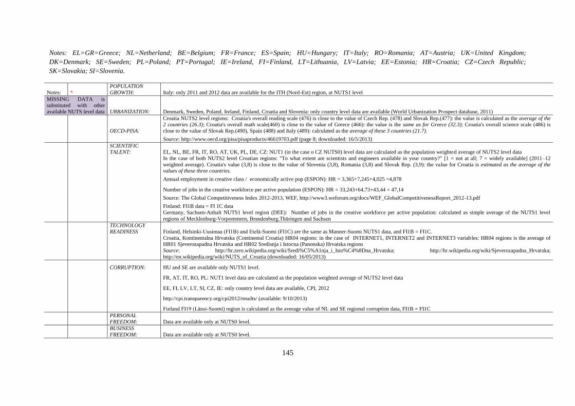
145
Notes: EL=GR=Greece; NL=Netherland; BE=Belgium; FR=France; ES=Spain; HU=Hungary; IT=Italy; RO=Romania; AT=Austria; UK=United Kingdom;
DK=Denmark; SE=Sweden; PL=Poland; PT=Portugal; IE=Ireland, FI=Finland, LT=Lithuania, LV=Latvia; EE=Estonia; HR=Croatia; CZ=Czech Republic;
SK=Slovakia; SI=Slovenia.
Notes: *
POPULATION
GROWTH: Italy: only 2011 and 2012 data are available for the ITH (Nord-Est) region, at NUTS1 level
MISSING DATA is substituted with other
available NUTS level data URBANIZATION: Denmark, Sweden, Poland, Ireland, Finland, Croatia and Slovenia: only country level data are available (World Urbanization Prospect database, 2011)
OECD-PISA:
Croatia NUTS2 level regions: Croatia's overall reading scale (476) is close to the value of Czech Rep. (478) and Slovak Rep.(477): the value is calculated as the average of the
2 countries (26.3); Croatia's overall math scale(460) is close to the value of Greece (466): the value is the same as for Greece (32.3); Croatia's overall science scale (486) is
close to the value of Slovak Rep.(490), Spain (488) and Italy (489): calculated as the average of these 3 countries (21.7).
Source: http://www.oecd.org/pisa/pisaproducts/46619703.pdf (page 8; downloaded: 16/5/2013)
SCIENTIFIC TALENT: EL, NL, BE, FR, IT, RO, AT, UK, PL, DE, CZ: NUT1 (in the case o CZ NUTS0) level data are calculated as the population weighted average of NUTS2 level data
In the case of both NUTS2 level Croatian regions: "To what extent are scientists and engineers available in your country?" [1 = not at all; 7 = widely available] (2011–12
weighted average). Croatia's value (3,8) is close to the value of Slovenia (3,8), Romania (3,8) and Slovak Rep. (3,9): the value for Croatia is estimated as the average of the values of these three countries.
Annual employment in creative class / economically active pop (ESPON): HR = 3,365+7,245+4,025 =4,878
Number of jobs in the creative workforce per active population (ESPON): HR = 33,243+64,73+43,44 = 47,14
Source: The Global Competitiveness Index 2012-2013, WEF, http://www3.weforum.org/docs/WEF_GlobalCompetitivenessReport_2012-13.pdf
Finland: FI1B data = FI 1C data
Germany, Sachsen-Anhalt NUTS1 level region (DEE): Number of jobs in the creative workforce per active population: calculated as simple average of the NUTS1 level
regions of Mecklenburg-Vorpommern, Brandenburg,Thüringen and Sachsen
TECHNOLOGY
READINESS Finland, Helsinki-Uusimaa (FI1B) and Etelä-Suomi (FI1C) are the same as Manner-Suomi NUTS1 data, and FI1B = FI1C.
Croatia, Kontinentalna Hrvatska (Continental Croatia) HR04 regions: in the case of INTERNET1, INTERNET2 and INTERNET3 variables: HR04 regions is the average of HR01 Sjeverozapadna Hrvatska and HR02 Sredisnja i Istocna (Panonska) Hrvatska regions
Source: http://hr.zero.wikipedia.org/wiki/Sredi%C5%A1nja_i_Isto%C4%8Dna_Hrvatska; http://hr.wikipedia.org/wiki/Sjeverozapadna_Hrvatska;
http://en.wikipedia.org/wiki/NUTS_of_Croatia (downloaded: 16/05/2013)
CORRUPTION: HU and SE are available only NUTS1 level.
FR, AT, IT, RO, PL: NUT1 level data are calculated as the population weighted average of NUTS2 level data
EE, FI, LV, LT, SI, CZ, IE: only country level data are available, CPI, 2012
http://cpi.transparency.org/cpi2012/results/ (available: 9/10/2013)
Finland FI19 (Länsi-Suomi) region is calculated as the average value of NL and SE regional corruption data, FI1B = FI1C
PERSONAL
FREEDOM: Data are available only at NUTS0 level.
BUSINESS
FREEDOM: Data are available only at NUTS0 level.

146
EU QoG INDEX: HU and SE are available only NUTS1 level.
FR, AT, IT, RO, PL: NUT1 level data are calculated as the population weighted average of NUTS2 level data
IE, FI, SI: only country level data are available
HR: estimated, the average of the values of SP, CZ, SL, HU, RO, EL, IT. For the estimation, the following WEF data were used:
Burden of government regulation: How burdensome is it for businesses in your country to comply with governmental administrative requirements (e.g., permits, regulations, reporting)? [1 = extremely; 7 =
extremely easy] | 2011–12 weighted average
Transparency of government policymaking: Transparency of government policymaking: How easy is it for businesses in your country to obtain information about changes in government policies and regulations affecting their activities? [1 = impossible; 7 =
extremely easy] | 2011–12 weighted average
Government provision of services for improved business performance: To what extent does the government in your country continuously improve its provision of services to help businesses in your country boost their economic performance? [1 = impossible; 7 =
extremely easy] | 2011–12 weighted average
Source: The Global Competitiveness Index 2012-2013, WEF, http://www3.weforum.org/docs/WEF_GlobalCompetitivenessReport_2012-13.pdf
FIRM-LEVEL
TECHNOLOGY ABSORPTION Data are available only at NUTS0 level.
EMPLOYMENT IN
KNOWLEDGE-INTENSIVE AND
HIGH-
TECHNOLOGY ADOPTIONS:
Employment in High-Technology Adoptions: DE5= average of DE2 and DE6; PT15= average of PT17 and PT18; Employment in knowledge intensive sectors: DE5= average
of DE2 and DE6; DEC= same as DE3; PT15= average of PT17 and PT18; PT18= average of PT16 and PT17; ES23= same as ES24; Researchers: missing data: GR, FR
NATURE OF
COMPETITIVE
ADVANTAGE Data are available only at NUTS0 level.
BUSINESS
SOPHISTICATION:
In the case of GVA in JK sectors and FDI intensity: EL, NL, BE, FR, IT, RO, AT, UK, PL, DE, CZ: NUT1 (in the case o CZ NUTS0) level data are calculated as the
population weighted average of NUTS2 level data
HR: estimated, the average of the values of SI01 and SI02
TECHNOLOGY TRANSFER: High-tech patents: ES23= same as ES24; ES43= same as ES13; PT18= average of PT16 and PT17; SK03= average of SK02 and SK04
PCT patent indicator and PCT patent for biotechnology indicator: no data are available for LV, LT, RO. FR, AT, IT, PL : NUT1 level data are calculated as the population
weighted average of NUTS2 level data
HR: estimated as the average of HU, CZ, EL, LT, SK, PL. For the estimation, the following WEF data were used:
PCT patent application: Number of applications filed under the Patent Cooperation Treaty (PCT) per million population | 2008–09 average
Source: The Global Competitiveness Index 2012-2013, WEF, http://www3.weforum.org/docs/WEF_GlobalCompetitivenessReport_2012-13.pdf
GERD: HR, Kontinentalna Hrvatska (Continental Croatia) HR04 regions:HR04 regions is the average of HR01 Sjeverozapadna Hrvatska and HR02 Sredisnja i Istocna (Panonska) Hrvatska regions
Finland: FI1B data = FI 1C data; FI1D = average of Pohjois-Suomi and Itä-Suomi
CLUSTERING: SI, DK: Clusters variable are available only for country level (NUTS0 level).
CZ, BE, DE, EL, FR, IT, NL, AT, PL, RO, UK : NUT1 (in the case o CZ NUTS0) level data are calculated as the population weighted average of NUTS2 level data

147
Finland: FI1B data = FI 1C data
HR = average of the values of HU, PL, LV. For the estimation, the following WEF data were used:
State of cluster development: In your country’s economy, how prevalent are well-developed and deep clusters? [1 = nonexistent; 7 = widespread in many fields] | 2011–12 weighted average
Source: The Global Competitiveness Index 2012-2013, WEF, http://www3.weforum.org/docs/WEF_GlobalCompetitivenessReport_2012-13.pdf
CONNECTIVIY: EL, NL, BE, FR, IT, RO, AT, UK, PL, DE: NUT1 level data are calculated as the population weighted average of NUTS2 level data
HR: ROAD = average of LT, IE, EE, SI; RAILROAD = average of SI, HU, EE; AIR = average of EE, HU, LT. For the estimation, the following WEF data were used:
CZ= ROAD = average of SK, EL, HU, RAILROAD = average of SK, LT, DK; AIR = average of UK, AT, IE, DK, SE, BE. For the estimation, the following WEF data were used:
ROAD: Croatia two regions: Quality of road infrastructure: How would you assess the road system in your country? [1 = extremely underdeveloped; 7 = extensive and efficient
by international standards] | 2011–12 weighted, average of the ROAD variables of Lithuania, Ireland, Estonia and Slovenia.
RAILROAD: Croatia two regions: Quality of railroad infrastructure: How would you assess the railroad system in your country? [1 = extremely underdeveloped; 7 = extensive
and efficient by international standards] | 2011–12 weighted, average of the railroad variables of Slovenia, Estonia, Hungary
AIR: Croatia two regions: Quality of air transport infrastructure: How would you assess passenger air transport infrastructure in your country? [1 = extremely underdeveloped; 7 = extensive and efficient by international standards] |2011–12 weighted average, average of the AIR variables of Estonia, Lithuania and Hungary
Source: The Global Competitiveness Index 2012-2013, WEF, http://www3.weforum.org/docs/WEF_GlobalCompetitivenessReport_2012-13.pdf
DCM: Data are available only at NUTS0 level.
CONCENTRATION OF FINANCIAL
SERVICES: HR: average of SI, EL, IE, LT. For the estimation, the following WEF data were used:
Availability of financial services: Does the financial sector in your country provide a wide variety of financial products and services to businesses? [1 = not at all; 7 = provides a wide variety] | 2011–12
Source: The Global Competitiveness Index 2012-2013, WEF, http://www3.weforum.org/docs/WEF_GlobalCompetitivenessReport_2012-13.pdf
Finland, FI1B = FI1C
SI: only NUTS0 level data are available.
No data
Share of Product Innovation (used as
individual variable) DE: Brandenburg: Share of knowledge workers, calculated as simple average of the Mecklenburg-Vorpommern, Sachsen-Anhalt,Thüringen and Sachsen
HR: average of PL, LV, LT, RO, SK. or the estimation, the following WEF data were used:
Capacity for innovation: In your country, how do companies obtain technology? [1 = exclusively from licensing or imitating foreign companies; 7 = by conducting formal
research and pioneering
Source: The Global Competitiveness Index 2012-2013, WEF, http://www3.weforum.org/docs/WEF_GlobalCompetitivenessReport_2012-13.pdf
Share of Process Innovation (used as
individual variable) DE: Brandenburg: Share of knowledge workers, calculated as simple average of the Mecklenburg-Vorpommern, Sachsen-Anhalt,Thüringen and Sachsen
HR: average of PL, LV, LT, RO, SK. or the estimation, the following WEF data were used:
Capacity for innovation: In your country, how do companies obtain technology? [1 = exclusively from licensing or imitating foreign companies; 7 = by conducting formal research and pioneering
Source: The Global Competitiveness Index 2012-2013, WEF, http://www3.weforum.org/docs/WEF_GlobalCompetitivenessReport_2012-13.pdf
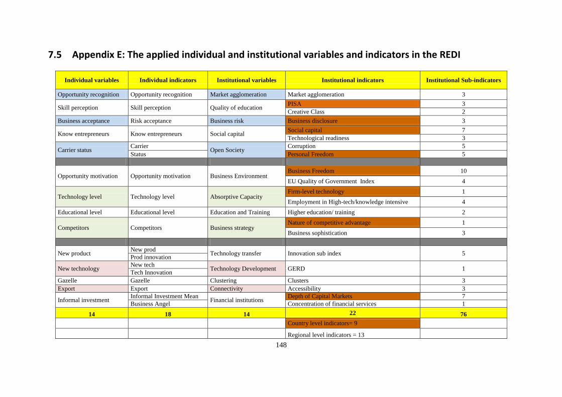
148
7.5 Appendix E: The applied individual and institutional variables and indicators in the REDI
Individual variables Individual indicators Institutional variables Institutional indicators Institutional Sub-indicators
Opportunity recognition Opportunity recognition Market agglomeration Market agglomeration 3
Skill perception Skill perception Quality of education PISA 3
Creative Class 2
Business acceptance Risk acceptance Business risk Business disclosure 3
Know entrepreneurs Know entrepreneurs Social capital Social capital 7
Technological readiness 3
Carrier status Carrier
Open Society Corruption 5
Status Personal Freedom 5
Opportunity motivation Opportunity motivation Business Environment Business Freedom 10
EU Quality of Government Index 4
Technology level Technology level Absorptive Capacity Firm-level technology 1
Employment in High-tech/knowledge intensive 4
Educational level Educational level Education and Training Higher education/ training 2
Competitors Competitors Business strategy Nature of competitive advantage 1
Business sophistication 3
New product New prod
Technology transfer Innovation sub index 5 Prod innovation
New technology New tech
Technology Development GERD 1 Tech Innovation
Gazelle Gazelle Clustering Clusters 3
Export Export Connectivity Accessibility 3
Informal investment Informal Investment Mean
Financial institutions Depth of Capital Markets 7
Business Angel Concentration of financial services 1
14 18 14 22 76
Country level indicators= 9
Regional level indicators = 13

149
7.6 Appendix F: The characteristics of the penalty function
In the previous version of the PFB, we have used the natural logarithm penalty function (, Acs et al.,
2013). Tarabusi and Palazzi (2004) and Tarabusi and Guarini (2012) have also developed a family of
penalization methodology. We can define the penalty as the difference between the original and the
after penalty pillar values. Following Tarabusi and Palazzi (2004) Tarabusi and Guarini (2012) and
Szerb et al. (2011) we can define the required characteristics of the penalty functions. Most
importantly, the penalty function should reflect to the magnitude of the penalty, lower difference
implies lower penalty while higher unbalance implies higher penalty. The penalty function should also
reflect to the compensation of the loss of one pillar for a gain in another pillar.
The Marginal Rate of Compensation (MRC) is defined as:
(E1)
Full compensability means that a loss in one pillar can be compensated by the same increase in
another pillar. However, this is not realistic. The MRC is the same concept as the Marginal Rate of
Substitution for goods and to the Marginal Rate of Technical Substitution of inputs (Tarabusi and
Guinari 2012), that are reflected to the law of diminishing return. Therefore, the effect of the change of
the penalty should not be proportional reflecting to the increasing rate of (MRC). It means that we
require higher compensation for the loss in one pillar if the difference between another pillar value and
the particular pillar is higher as compared to the situation when the difference between the pillars is
lower. The required positive value of the second derivative means that the pillars just only partially
and not fully compensable with each other. So the penalty should increase in an increasing rate:
(E2)
Tarabusi and Palazzi (2004) suggested a correction form of an exponential function of a . In a
recent article Tarabusi and Guarini (2012) used another adjustment function that refers to the deviation
from the mean pillar value. For our purposes the mean adjustment is not really suitable so it is better to
use the exponential form. Modifying Tarabusi and Palazzi (2004) original function for our purposes,
we can define a penalty function family as
(E3)
where is the modified, post-penalty value of index component j in region i
is the normalized value of index component j in region i
is the lowest value of for region i.
i = 1, 2,……n = the number of regions
j= 1, 2,.……m= the number of index components
a, and b are parameters are calibrated to be between 0 and 1 to provide the penalty from 0 to 1.
With the combination of the two parameters different kinds of penalty functions can be created.
Figures E1 and E2 show the effect of parameters “a” and “b”.

150
Figure 19. The effect of changing parameter a in the penalty function (ymin =0, and b=1)
Figure 20. The effect of changing parameter b in the penalty function (ymin =0, and a=1)
When parameter a =1 then the penalty is minimal: After the penalty, the 0.2 original pillar value is
going to be 0.18, so the penalty is 0.02. At higher pillar values the penalty is higher. If the original
pillar value is 1, then the penalized pillar value is 0.63, so the maximum penalty is 0.37. The decrease
of the parameter “a” has an effect of increasing penalty. For example, if parameter a=0.5 then the
maximum penalty is 0.68, at a=0.1 the maximum penalty is 0.94. At a=0, the maximum penalty is 1. It
means that the performance of the system is solely depending on the minimum pillar value. Since the
0
0,1
0,2
0,3
0,4
0,5
0,6
0,7
0,8
0,9
1
0 0,2 0,4 0,6 0,8 1
a=1 a=0,5 a=0,1
0
0,1
0,2
0,3
0,4
0,5
0,6
0,7
0,8
0,9
1
0 0,2 0,4 0,6 0,8 1
b=1 b=0,5 b=0,1

151
minimum pillar value here is 0, all the other penalized pillar values are also restricted to be 0 from the
system perspective.
7.7 Appendix G: The calculation of the REDI scores
1. Pillar values were capped at the 95 percent value. By the application of this technique we got a
proper benchmarking for each of the pillars. In this case not a potential outlier serves as a
reference, but at least the best six regions have the same maximum value.
2. Capped pillar values were normalized by using the distance method. While this method
transforms variables to be in the [0,1] range, does not restrict the worse region to have a zero
value as in the case of the min-max normalization.
(F1)
for all j= 1,..m the number of pillars
where is the normalized score value for region i and pillar j
is the original pillar value for region i and pillar j
is the maximum value for pillar j
3. Original normalized pillar value averages range from 0,38 (Opportunity Perception and
Financing) to 0,63 (Product Innovation). We believed that these values reflect to the difficulty
to reach good performance; i.e. it is more difficult to attain good performance in Product
Innovation as compared to Finance. For proper public policy application we equated the
fourteen pillar averages to have the same marginal effect. While this technique does not
handle the cost differences over size and countries it definitely reduces potential biases.
The arithmetic average of pillar j for number n regions is:
(F2)
We want to transform the xi,j values such that the potential values to be in the [0,1] range.
, ,
k
i j i jy x (F3)
where k is the “strength of adjustment”, the k -th moment of jX is exactly the needed
average, jy . We have to find the root of the following equation for k :
,
1
0n
k
i j j
i
x ny
(F4)
It is easy to see based on previous conditions and derivatives that the function is decreasing
and convex which means it can be quickly solved using the well-known Newton-Raphson
method with an initial guess of 0. After obtaining k , the computations are straightforward.
Note that if
1
1
1
j j
j j
j j
x y k
x y k
x y k
that is k be thought of as the strength (and direction) of adjustment.

152
4. We have defined entrepreneurship as the dynamic interaction of entrepreneurial attitudes,
abilities, and aspiration across different levels of development. One issue this definition raises
is how to bring the system perspective of dynamic interaction into the model. Following the
Theory of Weakest Link and the Theory of Constraints we developed the Penalty for
Bottleneck method to determine the optimum configuration. We hold that all the fourteen
pillars constituting the system of entrepreneurship should be equal for optimalizing the use of
the available resources. The performance of a particular region depends on its worst
performing pillar, called the bottleneck. With respect to entrepreneurship, bottleneck means a
shortage or the lowest level of a particular entrepreneurial pillar, relative to other pillars. This
notion of a bottleneck is important for policy purposes. Our model suggests that pillars
interact; if they are out of balance, entrepreneurship is inhibited. The pillar values should be
adjusted in a way that takes into account this notion of balance. After normalizing the scores
of all the pillars, and equalizing the averages of the pillars the value of each pillar of a region
is penalized by linking it to the score of the pillar with the weakest performance in that region.
We defined our penalty function following as:
(F5)
where is the modified, post-penalty value of pillar j in region i
is the normalized value of index component j in region i
is the lowest value of for region i.
i = 1, 2,……n = the number of regions
j= 1, 2,.……m= the number of pillars
5. The pillars are the basic building blocks of the sub-index: entrepreneurial attitudes,
entrepreneurial abilities, and entrepreneurial aspirations. The value of a sub-index for any
country is the arithmetic average of its PFB-adjusted pillars for that sub-index multiplied by a
100. The maximum value of the sub-indices is 100 and the potential minimum is 0, both of
which reflect the relative position of a country in a particular sub-index.
where is the modified, post-penalty value of pillar j in region i
i = 1, 2,……n = the number of regions
j= 1, 2,.……14= the number of pillars
6. The super-index, the Regional Entrepreneurship and Development Index, is simply the
average of the three sub-indices.
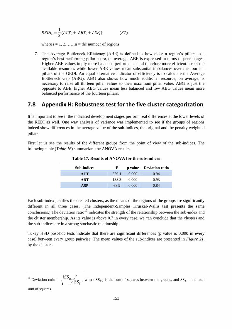
153
where i = 1, 2,……n = the number of regions
7. The Average Bottleneck Efficiency (ABE) is defined as how close a region’s pillars to a
region’s best performing pillar score, on average. ABE is expressed in terms of percentages.
Higher ABE values imply more balanced performance and therefore more efficient use of the
available resources while lower ABE values mean substantial imbalances over the fourteen
pillars of the GEDI. An equal alternative indicator of efficiency is to calculate the Average
Bottleneck Gap (ABG). ABG also shows how much additional resource, on average, is
necessary to raise all thirteen pillar values to their maximum pillar value. ABG is just the
opposite to ABE, higher ABG values mean less balanced and low ABG values mean more
balanced performance of the fourteen pillars.
7.8 Appendix H: Robustness test for the five cluster categorization
It is important to see if the indicated development stages perform real differences at the lower levels of
the REDI as well. One way analysis of variance was implemented to see if the groups of regions
indeed show differences in the average value of the sub-indices, the original and the penalty weighted
pillars.
First let us see the results of the different groups from the point of view of the sub-indices. The
following table (Table 16) summarizes the ANOVA results.
Table 17. Results of ANOVA for the sub-indices
Sub-indices F p value Deviation ratio
ATT 220.1 0.000 0.94
ABT 188.3 0.000 0.93
ASP 68.9 0.000 0.84
Each sub-index justifies the created clusters, as the means of the regions of the groups are significantly
different in all three cases. (The Independent-Samples Kruskal-Wallis test presents the same
conclusions.) The deviation ratio12
indicates the strength of the relationship between the sub-index and
the cluster membership. As its value is above 0.7 in every case, we can conclude that the clusters and
the sub-indices are in a strong stochastic relationship.
Tukey HSD post-hoc tests indicate that there are significant differences (p value is 0.000 in every
case) between every group pairwise. The mean values of the sub-indices are presented in Figure 21.
by the clusters.
12 Deviation ratio =
T
BG
SSSS
, where SSBG is the sum of squares between the groups, and SST is the total
sum of squares.

154
Figure 21. The comparison of the mean of the sub-indices by cluster membership
Moving on with the analysis, we examine the situation of the penalty adjusted pillars. The results of
the one-way analysis of variance seem to support our classification (Table 17).
Table 18. Results of ANOVA for the penalty weighted pillar values
Penalty weighted pillars F p value Deviation ratio
Opportunity perception 64.2 0.000 0.83
Startup skills 50.3 0.000 0.79
Risk Acceptance 28.8 0.000 0.70
Networking 88.4 0.000 0.86
Cultural support 68.0 0.000 0.83
Opportunity startup 78.2 0.000 0.85
Technology adoption 75.1 0.000 0.85
Human capital 41.0 0.000 0.76
Competition 96.8 0.000 0.87
Product innovation 34.5 0.000 0.73
Process innovation 12.6 0.000 0.54
High growth 22.1 0.000 0.65
Globalization 10.2 0.000 0.50
Financing 26.4 0.000 0.68
According to the p values (p = 0.000), the pillars and the clusters are not independent meaning that the
mean values are different among the five groups. (The Independent-Samples Kruskal-Wallis test
presents the same conclusions.) The strength of the stochastic relationships between the pillars and the
cluster membership are still strong in most of the cases. There are only four pillars, where the strength
of the relationship is moderate (Process innovation, High growth, Globalisation and Financing).
However, even the lowest value is above 0.5. Pairwise comparison was carried out to see the
underlying structure of the different pillars. Table 18 summarizes the p values of the Tukey HSD post-
hoc tests.
0
10
20
30
40
50
60
70
80
Highest High Moderate Low Lowest
ATT
ABT
ASP
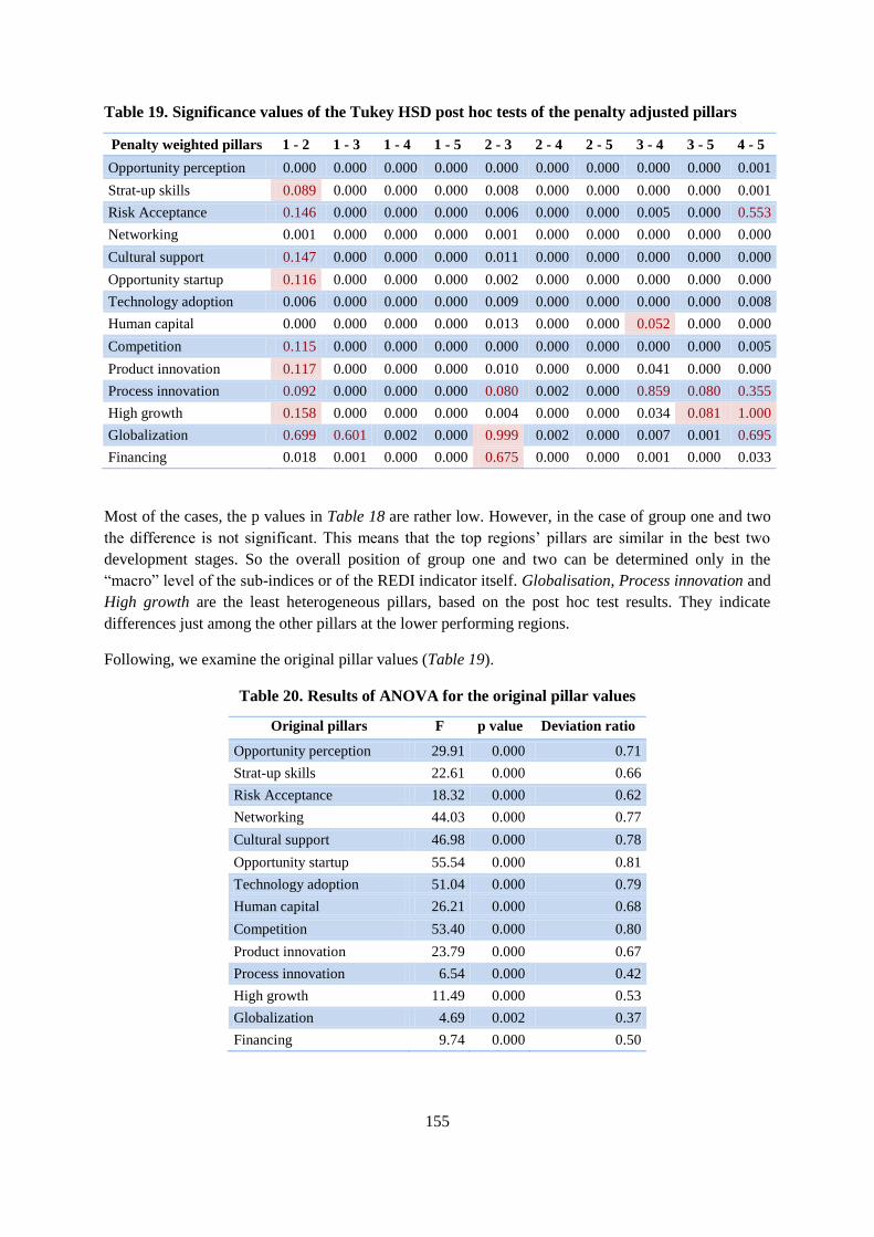
155
Table 19. Significance values of the Tukey HSD post hoc tests of the penalty adjusted pillars
Penalty weighted pillars 1 - 2 1 - 3 1 - 4 1 - 5 2 - 3 2 - 4 2 - 5 3 - 4 3 - 5 4 - 5
Opportunity perception 0.000 0.000 0.000 0.000 0.000 0.000 0.000 0.000 0.000 0.001
Strat-up skills 0.089 0.000 0.000 0.000 0.008 0.000 0.000 0.000 0.000 0.001
Risk Acceptance 0.146 0.000 0.000 0.000 0.006 0.000 0.000 0.005 0.000 0.553
Networking 0.001 0.000 0.000 0.000 0.001 0.000 0.000 0.000 0.000 0.000
Cultural support 0.147 0.000 0.000 0.000 0.011 0.000 0.000 0.000 0.000 0.000
Opportunity startup 0.116 0.000 0.000 0.000 0.002 0.000 0.000 0.000 0.000 0.000
Technology adoption 0.006 0.000 0.000 0.000 0.009 0.000 0.000 0.000 0.000 0.008
Human capital 0.000 0.000 0.000 0.000 0.013 0.000 0.000 0.052 0.000 0.000
Competition 0.115 0.000 0.000 0.000 0.000 0.000 0.000 0.000 0.000 0.005
Product innovation 0.117 0.000 0.000 0.000 0.010 0.000 0.000 0.041 0.000 0.000
Process innovation 0.092 0.000 0.000 0.000 0.080 0.002 0.000 0.859 0.080 0.355
High growth 0.158 0.000 0.000 0.000 0.004 0.000 0.000 0.034 0.081 1.000
Globalization 0.699 0.601 0.002 0.000 0.999 0.002 0.000 0.007 0.001 0.695
Financing 0.018 0.001 0.000 0.000 0.675 0.000 0.000 0.001 0.000 0.033
Most of the cases, the p values in Table 18 are rather low. However, in the case of group one and two
the difference is not significant. This means that the top regions’ pillars are similar in the best two
development stages. So the overall position of group one and two can be determined only in the
“macro” level of the sub-indices or of the REDI indicator itself. Globalisation, Process innovation and
High growth are the least heterogeneous pillars, based on the post hoc test results. They indicate
differences just among the other pillars at the lower performing regions.
Following, we examine the original pillar values (Table 19).
Table 20. Results of ANOVA for the original pillar values
Original pillars F p value Deviation ratio
Opportunity perception 29.91 0.000 0.71
Strat-up skills 22.61 0.000 0.66
Risk Acceptance 18.32 0.000 0.62
Networking 44.03 0.000 0.77
Cultural support 46.98 0.000 0.78
Opportunity startup 55.54 0.000 0.81
Technology adoption 51.04 0.000 0.79
Human capital 26.21 0.000 0.68
Competition 53.40 0.000 0.80
Product innovation 23.79 0.000 0.67
Process innovation 6.54 0.000 0.42
High growth 11.49 0.000 0.53
Globalization 4.69 0.002 0.37
Financing 9.74 0.000 0.50

156
The p values are below 0.01 in every case, reinforcing the proper selection of such categorization
(Table 19). (The Independent-Samples Kruskal-Wallis test presents the same conclusions.) However,
the strength of the relationships is not so convincing. Six pillars still indicate strong stochastic
relationship (Opportunity perception, Networking, Cultural support, Opportunity startup, Technology
adoption and Competition). All the other pillars show medium-strong relationship. Pairwise
comparison is necessary again to see the significance of the differences between the five clusters.
Table 20 summarizes the p values of the Tukey HSD post-hoc tests. The red cells include those p
values that are above 0.05. So in these cases the pairwise comparisons show that the five clusters are
independent from each other. The differences between clusters 1 and 2, 2 and 3, and 4 and 5 indicate
the least significant differences. Similarly to the earlier results, Globalisation is found to be the most
homogeneous original pillar. Process innovation and High growth are also less heterogeneous as
compared to the other pillars.
Table 21. Significance values of the Turkey HSD post-hoc tests of the original pillar values
Original pillars 1 - 2 1 - 3 1 - 4 1 - 5 2 - 3 2 - 4 2 - 5 3 - 4 3 - 5 4 - 5
Opportunity perception 0.012 0.000 0.000 0.000 0.035 0.000 0.000 0.005 0.000 0.293
Strat-up skills 0.639 0.031 0.000 0.000 0.137 0.000 0.000 0.005 0.000 0.116
Risk Acceptance 0.648 0.014 0.000 0.000 0.050 0.000 0.000 0.012 0.006 0.947
Networking 0.026 0.000 0.000 0.000 0.035 0.000 0.000 0.000 0.000 0.159
Cultural support 0.614 0.017 0.000 0.000 0.077 0.000 0.000 0.002 0.000 0.000
Opportunity startup 0.516 0.008 0.000 0.000 0.056 0.000 0.000 0.000 0.000 0.001
Technology adoption 0.003 0.000 0.000 0.000 0.156 0.000 0.000 0.000 0.000 0.083
Human capital 0.000 0.000 0.000 0.000 0.158 0.000 0.000 0.314 0.000 0.006
Competition 0.146 0.001 0.000 0.000 0.095 0.000 0.000 0.000 0.000 0.107
Product innovation 0.208 0.003 0.000 0.000 0.123 0.000 0.000 0.177 0.000 0.001
Process innovation 0.263 0.008 0.003 0.000 0.233 0.074 0.009 0.996 0.580 0.733
High growth 0.076 0.001 0.000 0.000 0.150 0.000 0.003 0.320 0.530 1.000
Globalization 0.966 0.999 0.206 0.058 0.983 0.154 0.031 0.050 0.010 0.828
Financing 0.040 0.060 0.000 0.000 1.000 0.019 0.011 0.016 0.009 0.950
The penalty adjusted pillars and the sub-indices clearly justify the results of the cluster analysis. The
five different groups (development stages) present significantly different mean values at the level of
the sub-indices and of the penalty weighted pillars. The level of the performance of the regions
seems to be captured correctly by the penalized pillars and the sub-indices. These facts
underline the results of the REDI index calculation methodology.
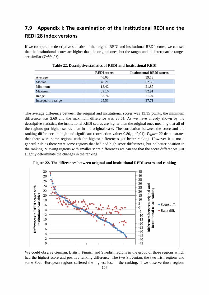
157
7.9 Appendix I: The examination of the Institutional REDI and the
REDI 28 index versions
If we compare the descriptive statistics of the original REDI and institutional REDI scores, we can see
that the institutional scores are higher than the original ones, but the ranges and the interquartile ranges
are similar (Table 21).
Table 22. Descriptive statistics of REDI and Institutional REDI
REDI scores Institutional REDI scores
Average 46.03 59.18
Median 48.21 62.50
Minimum 18.42 21.87
Maximum 82.16 92.91
Range 63.74 71.04
Interquartile range 25.51 27.71
The average difference between the original and institutional scores was 13.15 points, the minimum
difference was 2.69 and the maximum difference was 28.51. As we have already shown by the
descriptive statistics, the institutional REDI scores are higher than the original ones meaning that all of
the regions got higher scores than in the original case. The correlation between the score and the
ranking differences is high and significant (correlation value: 0.80, p=0,01). Figure 22 demonstrates
that there were some regions with the highest differences got better ranking. However it is not a
general rule as there were some regions that had had high score differences, but no better position in
the ranking. Viewing regions with smaller score differences we can see that the score differences just
slightly determinate the changes in the ranking.
Figure 22. The differences between original and institutional REDI scores and ranking
We could observe German, British, Finnish and Swedish regions in the group of those regions which
had the highest score and positive ranking difference. The two Slovenian, the two Irish regions and
some South-European regions suffered the highest lost in the ranking. If we observe those regions
-45
-40
-35
-30
-25
-20
-15
-10
-5
0
5
10
15
20
25
30
35
40
45
0
2
4
6
8
10
12
14
16
18
20
22
24
26
28
30
Dif
feren
ces
bet
wee
n o
rig
ina
l a
nd
inst
itu
tio
na
l R
ED
I ra
nk
ing
Dif
fere
nce
s in
RE
DI
sco
res
wit
h
inst
itu
tio
na
l v
ari
ab
les
Score diff.
Rank diff.
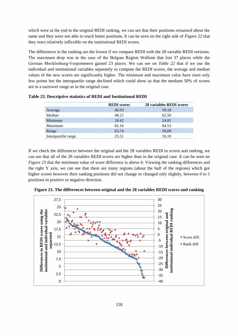
158
which were at the end in the original REDI ranking, we can see that their positions remained about the
same and they were not able to reach better positions. It can be seen on the right side of Figure 22 that
they react relatively inflexible on the institutional REDI scores.
The differences in the ranking are the lowest if we compare REDI with the 28 variable REDI versions.
The maximum drop was in the case of the Belgian Région Wallone that lost 37 places while the
German Mecklenburg-Vorpommern gained 23 places. We can see on Table 22 that if we use the
individual and institutional variables separately to compute the REDI scores, the average and median
values of the new scores are significantly higher. The minimum and maximum value have risen only
few points but the interquartile range declined which could show us that the medium 50% of scores
are in a narrower range as in the original case.
Table 23. Descriptive statistics of REDI and Institutional REDI
REDI scores 28 variables REDI scores
Average 46.03 59.18
Median 48.21 62.50
Minimum 18.42 24.81
Maximum 82.16 84.53
Range 63.74 59,09
Interquartile range 25.51 16,10
If we check the differences between the original and the 28 variables REDI in scores and ranking, we
can see that all of the 28 variables REDI scores are higher than in the original case. It can be seen on
Figure 23 that the minimum value of score difference is above 0. Viewing the ranking differences and
the right Y axis, we can see that there are many regions (about the half of the regions) which got
higher scores however their ranking positions did not change or changed only slightly, between 0 to 5
positions in positive or negative direction.
Figure 23. The differences between original and the 28 variables REDI scores and ranking
-40
-35
-30
-25
-20
-15
-10
-5
0
5
10
15
20
25
30
0
2,5
5
7,5
10
12,5
15
17,5
20
22,5
25
27,5
Dif
feren
ces
bet
wee
n o
rig
ina
l a
nd
inst
itu
tio
na
l-in
div
idu
al
RE
DI
ran
kin
g
Dif
feren
ces
in R
ED
I sc
ore
s u
sin
g t
he
inst
itu
tio
na
l a
nd
in
div
idu
al
va
ria
ble
s
sep
are
ted
Score diff.
Rank diff.
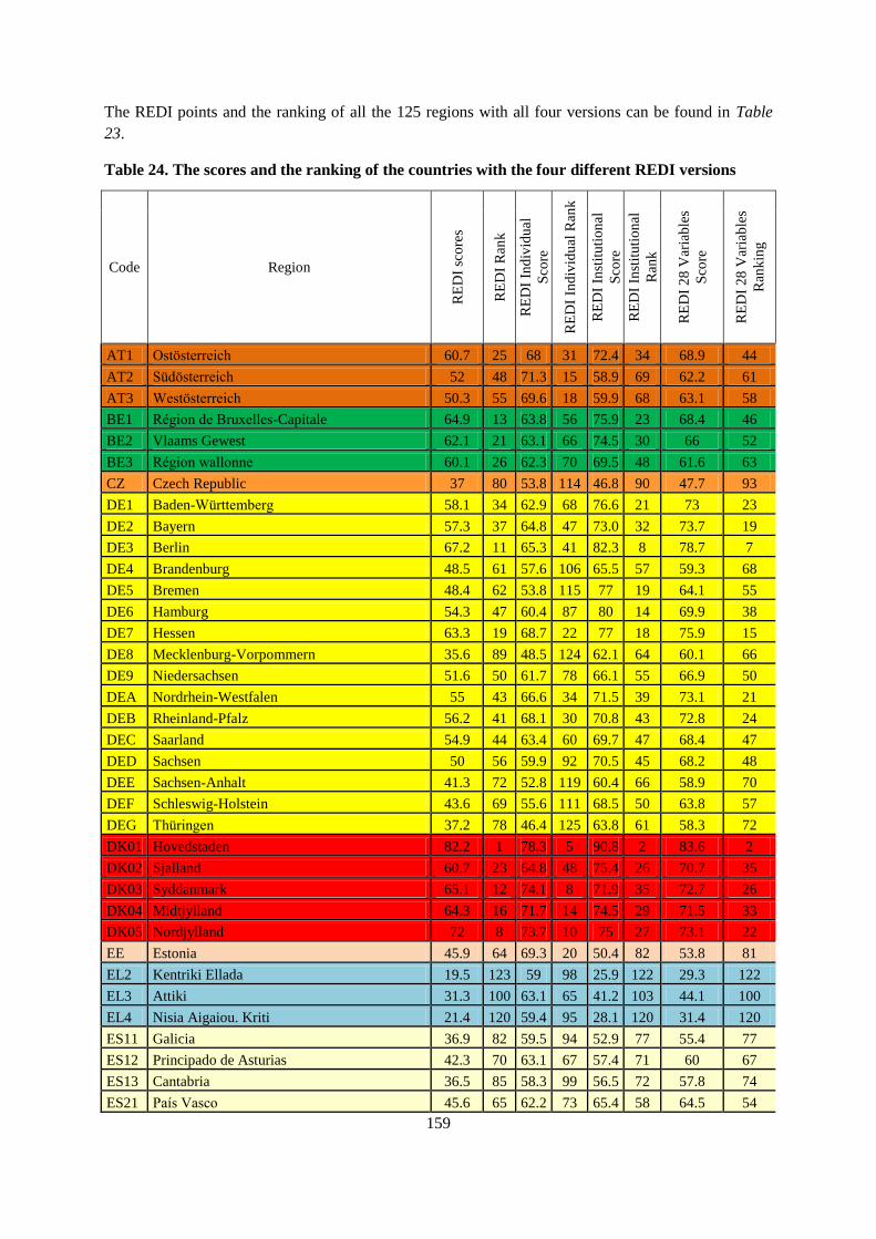
159
The REDI points and the ranking of all the 125 regions with all four versions can be found in Table
23.
Table 24. The scores and the ranking of the countries with the four different REDI versions
Code Region
RE
DI
sco
res
RE
DI
Ran
k
RE
DI
Ind
ivid
ual
Sco
re
RE
DI
Ind
ivid
ual
Ran
k
RE
DI
Inst
itu
tio
nal
Sco
re
RE
DI
Inst
itu
tio
nal
Ran
k
RE
DI
28
Var
iab
les
Sco
re
RE
DI
28
Var
iab
les
Ran
kin
g
AT1 Ostösterreich 60.7 25 68 31 72.4 34 68.9 44
AT2 Südösterreich 52 48 71.3 15 58.9 69 62.2 61
AT3 Westösterreich 50.3 55 69.6 18 59.9 68 63.1 58
BE1 Région de Bruxelles-Capitale 64.9 13 63.8 56 75.9 23 68.4 46
BE2 Vlaams Gewest 62.1 21 63.1 66 74.5 30 66 52
BE3 Région wallonne 60.1 26 62.3 70 69.5 48 61.6 63
CZ Czech Republic 37 80 53.8 114 46.8 90 47.7 93
DE1 Baden-Württemberg 58.1 34 62.9 68 76.6 21 73 23
DE2 Bayern 57.3 37 64.8 47 73.0 32 73.7 19
DE3 Berlin 67.2 11 65.3 41 82.3 8 78.7 7
DE4 Brandenburg 48.5 61 57.6 106 65.5 57 59.3 68
DE5 Bremen 48.4 62 53.8 115 77 19 64.1 55
DE6 Hamburg 54.3 47 60.4 87 80 14 69.9 38
DE7 Hessen 63.3 19 68.7 22 77 18 75.9 15
DE8 Mecklenburg-Vorpommern 35.6 89 48.5 124 62.1 64 60.1 66
DE9 Niedersachsen 51.6 50 61.7 78 66.1 55 66.9 50
DEA Nordrhein-Westfalen 55 43 66.6 34 71.5 39 73.1 21
DEB Rheinland-Pfalz 56.2 41 68.1 30 70.8 43 72.8 24
DEC Saarland 54.9 44 63.4 60 69.7 47 68.4 47
DED Sachsen 50 56 59.9 92 70.5 45 68.2 48
DEE Sachsen-Anhalt 41.3 72 52.8 119 60.4 66 58.9 70
DEF Schleswig-Holstein 43.6 69 55.6 111 68.5 50 63.8 57
DEG Thüringen 37.2 78 46.4 125 63.8 61 58.3 72
DK01 Hovedstaden 82.2 1 78.3 5 90.8 2 83.6 2
DK02 Sjalland 60.7 23 64.8 48 75.4 26 70.7 35
DK03 Syddanmark 65.1 12 74.1 8 71.9 35 72.7 26
DK04 Midtjylland 64.3 16 71.7 14 74.5 29 71.5 33
DK05 Nordjylland 72 8 73.7 10 75 27 73.1 22
EE Estonia 45.9 64 69.3 20 50.4 82 53.8 81
EL2 Kentriki Ellada 19.5 123 59 98 25.9 122 29.3 122
EL3 Attiki 31.3 100 63.1 65 41.2 103 44.1 100
EL4 Nisia Aigaiou. Kriti 21.4 120 59.4 95 28.1 120 31.4 120
ES11 Galicia 36.9 82 59.5 94 52.9 77 55.4 77
ES12 Principado de Asturias 42.3 70 63.1 67 57.4 71 60 67
ES13 Cantabria 36.5 85 58.3 99 56.5 72 57.8 74
ES21 País Vasco 45.6 65 62.2 73 65.4 58 64.5 54

160
Code Region
RE
DI
sco
res
RE
DI
Ran
k
RE
DI
Ind
ivid
ual
Sco
re
RE
DI
Ind
ivid
ual
Ran
k
RE
DI
Inst
itu
tio
nal
Sco
re
RE
DI
Inst
itu
tio
nal
Ran
k
RE
DI
28
Var
iab
les
Sco
re
RE
DI
28
Var
iab
les
Ran
kin
g
ES22 Comunidad Foral de Navarra 39 74 59.2 96 58.5 70 58 73
ES23 La Rioja 37.6 77 61.6 80 52 78 53.7 82
ES24 Aragón 32.6 95 58.1 102 48 89 51.3 88
ES30 Comunidad de Madrid 54.7 46 67.4 33 71 41 72.3 31
ES41 Castilla y León 36.8 83 59.9 91 54.2 76 56.4 76
ES42 Castilla-la Mancha 32.1 97 58.3 100 45.4 93 49 91
ES43 Extremadura 30.3 102 58 103 43.9 95 47.6 94
ES51 Cataluna 42.3 71 63.5 59 60.2 67 63.1 59
ES52 Comunidad Valenciana 38.1 75 61.4 83 55.6 74 57.4 75
ES53 Illes Balears 37.7 76 62 75 49.4 86 53 84
ES61 Andalucía 37.1 79 62.2 71 51.3 80 54.3 79
ES62 Región de Murcia 36.7 84 63.2 63 49.5 85 52.4 86
ES70 Canarias (ES) 35.5 90 63.7 57 48.5 88 52.2 87
FI19 Länsi-Suomi 58.7 32 68.7 23 71 42 72.4 29
FI1B Helsinki-Uusimaa 62.2 20 66.1 37 81.9 9 78.2 8
FI1C Etelä-Suomi 58.9 30 67.5 32 80.4 12 77.6 11
FI1D Pohjois- ja Ita-Suomi 51.2 52 61.7 79 71.6 37 70.6 36
FR1 Île de France 79.2 3 76 6 85.5 4 81.4 5
FR2 Bassin Parisien 50.9 54 65.1 43 62.5 62 61.6 62
FR3 Nord - Pas-de-Calais 48.8 60 62.1 74 68 52 64 56
FR4 Est (FR) 49.7 58 61 84 65.2 59 65.2 53
FR5 Ouest (FR) 51.8 49 64.8 46 61.1 65 62.8 60
FR6 Sud-Ouest (FR) 58.9 31 73.8 9 66.6 54 69.4 40
FR7 Centre-Est (FR) 64.2 17 71.2 16 73.5 31 70 37
FR8 Méditerranée 59.4 27 72.3 13 70.6 44 72.4 30
HR03 Jadranska Hrvatska (Adriatic Croatia) 32 98 68.3 27 36.8 107 40.4 107
HR04 Kontinentalna Hrvatska (Continental Croatia) 29.9 103 63.9 54 37.2 106 40.8 106
HU10 Közép-Magyarország 31.4 99 57.8 105 46.7 91 50 90
HU21 Közép-Dunántúl 22 117 55.9 109 33.8 113 37.4 113
HU22 Nyugat-Dunántúl 21.5 118 55.1 112 35.7 111 39.5 110
HU23 Dél-Dunántúl 23.8 113 57.9 104 36.3 109 40.1 108
HU31 Észak-Magyarország 22.4 115 57 107 32 115 35.7 115
HU32 Észak-Alföld 21.4 119 56 108 33.6 114 37.3 114
HU33 Dél-Alföld 21 121 52.6 120 34.8 112 38.6 112
IE01 Border. Midland and Western 63.4 18 80.3 2 66.1 56 69 43
IE02 Southern and Eastern 72 7 79.3 4 75.7 24 78 9
ITC Nord-Ovest 40.4 73 64.3 51 55.5 75 58.8 71
ITF Sud 27.3 109 63.2 64 36 110 38.7 111
ITG Isole 27.6 108 65.5 39 37.8 105 41.3 104
ITH Nord-Est 36.1 86 62.2 72 51.8 79 54.4 78

161
Code Region
RE
DI
sco
res
RE
DI
Ran
k
RE
DI
Ind
ivid
ual
Sco
re
RE
DI
Ind
ivid
ual
Ran
k
RE
DI
Inst
itu
tio
nal
Sco
re
RE
DI
Inst
itu
tio
nal
Ran
k
RE
DI
28
Var
iab
les
Sco
re
RE
DI
28
Var
iab
les
Ran
kin
g
ITI Centro (IT) 36.9 81 64.3 52 50.2 83 53.9 80
LT Lithuania 35.2 91 61.8 77 43.3 98 46.9 95
LV Latvia 33.8 93 68.3 28 42 100 45.7 97
NL1 Noord-Nederland 51.1 53 64.2 53 64.3 60 66.9 51
NL2 Oost-Nederland 56.5 39 65.9 38 68.4 51 70.8 34
NL3 West-Nederland 64.4 15 73.5 11 74.5 28 76.9 13
NL4 Zuid-Nederland 57 38 68.4 25 69.8 46 72.4 28
PL1 Region Centralny 36.1 88 51.9 121 50.9 81 50.2 89
PL2 Region Poludniowy 34.1 92 52.9 118 45.8 92 46.1 96
PL3 Region Wschodni 29.2 105 53.6 116 41.7 101 43.5 101
PL4 Region Pólnocno-Zachodni 32.3 96 51.5 122 43.3 99 43.5 102
PL5 Region Poludniowo-Zachodni 36.1 87 61.6 81 45.3 94 49 92
PL6 Region Pólnocny 33.2 94 55.1 113 43.7 96 45.2 98
PT11 Norte 29.2 106 59.5 93 37.9 104 41.3 103
PT15 Algarve 30.9 101 61.5 82 41.5 102 45 99
PT16 Centro (PT) 27.6 107 55.6 110 36.4 108 39.9 109
PT17 Lisboa 44.6 67 61.8 76 62.5 63 60.8 65
PT18 Alentejo 29.4 104 49.8 123 43.7 97 40.8 105
RO1 Macroregiunea unu 19.4 124 60.1 88 24.2 124 27.3 124
RO2 Macroregiunea doi 18.4 125 59.9 90 21.9 125 24.8 125
RO3 Macroregiunea trei 22.1 116 60.7 85 27.8 121 30.5 121
RO4 Macroregiunea patru 19.7 122 53.2 117 24.2 123 27.4 123
SE11 Stockholm 73.8 4 68.8 21 92.9 1 82.5 3
SE12 Östra Mellansverige 72.7 5 70.5 17 81.1 11 77.6 10
SE21 Smaland med öarna 49.9 57 63.2 62 69.4 49 68.6 45
SE22 Sydsverige 67.3 10 66.4 35 84.4 6 76.5 14
SE23 Vastsverige 72.2 6 72.5 12 80.1 13 80.1 6
SE31 Norra Mellansverige 57.7 36 68.6 24 67 53 67.1 49
SE32 Mellersta Norrland 48.2 63 58.2 101 71.5 40 61.4 64
SE33 Övre Norrland 64.7 14 68.4 26 76.7 20 73.1 20
SI01 Vzhodna Slovenija 45.3 66 81 1 49.9 84 53.5 83
SI02 Zahodna Slovenija 51.3 51 79.8 3 55.6 73 59 69
SK01 Bratislavsky kraj 44 68 69.5 19 49.3 87 52.4 85
SK02 Západné Slovensko 25.8 110 63.2 61 31.1 116 34.7 116
SK03 Stredné Slovensko 24.9 111 63.9 55 30.3 118 33.9 118
SK04 Vychodné Slovensko 24.5 112 59 97 30.9 117 34.6 117
UKC North East (UK) 48.9 59 60.5 86 72.7 33 69.2 42
UKD North West (UK) 59 28 63.7 58 81.7 10 74.6 17
UKE Yorkshire and The Humber 56.4 40 65.5 40 75.4 25 72.7 25
UKF East Midlands (UK) 55.3 42 62.8 69 77.9 16 72.7 27

162
Code Region
RE
DI
sco
res
RE
DI
Ran
k
RE
DI
Ind
ivid
ual
Sco
re
RE
DI
Ind
ivid
ual
Ran
k
RE
DI
Inst
itu
tio
nal
Sco
re
RE
DI
Inst
itu
tio
nal
Ran
k
RE
DI
28
Var
iab
les
Sco
re
RE
DI
28
Var
iab
les
Ran
kin
g
UKG West Midlands (UK) 58.6 33 64.7 49 76.5 22 71.8 32
UKH East of England 61.5 22 64.4 50 82.7 7 77.3 12
UKI London 79.9 2 74.8 7 85 5 84.5 1
UKJ South East (UK) 69.5 9 68.1 29 89.9 3 82.4 4
UKK South West (UK) 60.7 24 65 45 77.5 17 75.6 16
UKL Wales 54.7 45 65.1 44 71.7 36 69.8 39
UKM Scotland 59 29 65.2 42 78.3 15 74.2 18
UKN Northern Ireland (UK) 58 35 66.3 36 71.6 38 69.3 41

163
7.10 Appendix J: The effect of changing variables
During the creation of the REDI scores we have conducted hundreds of index versions. We also
recognized that the change of the variables or pillars had minimal influence on the ranking. Here, we
report the result of changing two variables. First, we replaced the original Clustering variable with the
“cluster observatory star rating” and with the “cluster employment” variable. Second, we calculated
the REDI scores with “Corruption” and “Personal freedom” instead of “Cultural support” variable.
Table 24 shows the Pearson’s correlation coefficient (between the original and new scores) and
Spearman’s rank correlation coefficient (between the original and new rankings).
Table 25. Correlation values between the original and new versions of REDI
Pearson’s coefficient 1 2 3 4 5
1 REDI 1 0.990 0.985 0.999 0.997
2 REDI Star rating
1 0.993 0.990 0.987
3 REDI Employment
1 0.985 0.982
4 REDI Corruption
1 0.996
5 REDI Personal Freedom
1
Spearman’s rho (new rankings to
the original one) 1 0.988 0.987 0.996 0.996
According to Table 24, all the changed versions of REDI scores correlate significantly on a very high
level with the original REDI scores and there are only very small differences between the new
versions. The Spearman’s rhos also prevail high rank correlation between any two of the reported
versions.
The Star rating, known as “Observatory star rating” is reported by the European Cluster Observatory.
Observatory star rating (or Star indicator) is the amount and quality of knowledge circulating and
spilling over between firms located in a given cluster. It depends upon the cluster size, the degree to
which it is specialized and the extent to which the locality (the region) is geared towards and focused
upon production in the relevant industries comprising the cluster. These three factors -- size,
specialization and focus –reflect whether the cluster has reached ‘specialized critical mass’ to develop
positive spillovers and linkages. The European Cluster Observatory assigns one, two or three stars to a
region depending on the extent to which clusters have achieved a specialized critical mass of the
following three factors:
1. Size: if employment reaches a sufficient share of total European employment, it is more likely
that meaningful economic effects of clusters will be present. The 'size' measure shows whether
a cluster is in the top 10% of all clusters in Europe within the same cluster category in terms of
the number of employees. Those in the top 10% will receive one star.
2. Specialisation: if a region is more specialized in a specific cluster category than the overall
economy across all regions, this is likely to be an indication that the economic effects of the
regional cluster have been strong enough to attract related economic activity from other
regions to this location, and these spillovers and linkages will be stronger. The 'specialisation'
measure compares the proportion of employment in a cluster category in a region over the
total employment in the same region, to the proportion of total European employment in that
cluster category over total European employment (see equation). If a cluster category in a
region has a specialization quotient of 2 or more it receives a star.

164
3. Focus: if a cluster accounts for a larger share of a region's overall employment, it is more
likely that spill-over effects and linkages will actually occur instead of being drowned in the
economic interaction of other parts of the regional economy. The 'focus' measure shows the
extent to which the regional economy is focused upon the industries comprising the cluster
category. This measure relates employment in the cluster to total employment in the region.
The top 10% of clusters which account for the largest proportion of their region's total
employment receive a star.
For practical use, we re-scaled the original 0-3 range variable to a scale of 0-10. Table 25 present the
basic statistics for the original REDI and the REDI Star rating versions. The differences are minimal.
Table 26. The descriptive statistics of the original and “Star rating” REDI versions
REDI REDI Star rating
Average 46.03 45.26
Median 48.21 46.33
Minimum 18.42 19.76
Maximum 82.16 80.61
Range 63.74 60.85
Interquartile range 25.51 23.34
The highest score difference was in the case of the Portugal Norte region (+3 points) and the lowest
score difference was noticed in the Danish Nordjylland region (-17.9 points). However, most of the
score differences were inside -3 points to +3 points a range. This differences for all the 125 regions
can be seen in Figure 24. Because of the small differences we did not need to apply a secondary
(right) Y axis.
Figure 24. Differences between REDI and “Star rating” REDI scores and ranking
Comparing the rankings, there are four regions that were the “winner” of the new ranking and gained 9
places: the Italian Nord-Est (from 86th to 77
th), the German Hamburg (from 47
th to 38
th), the Swedish
Norra Mellansverige (from 36th to 27
th) and the Finnish Länsi-Suomi (from 32
nd to 23
rd). The main
losers in the new ranking were two Danish regions that lost relatively high scores. Nordjylland lost 33
places (from 8th to 41
st) and Syddanmark’s position declined by 31 places (from 12
th to 43
rd).
-35
-32,5
-30
-27,5
-25
-22,5
-20
-17,5
-15
-12,5
-10
-7,5
-5
-2,5
0
2,5
5
7,5
10
Score diff. Starrating
Rank diff. Starrating
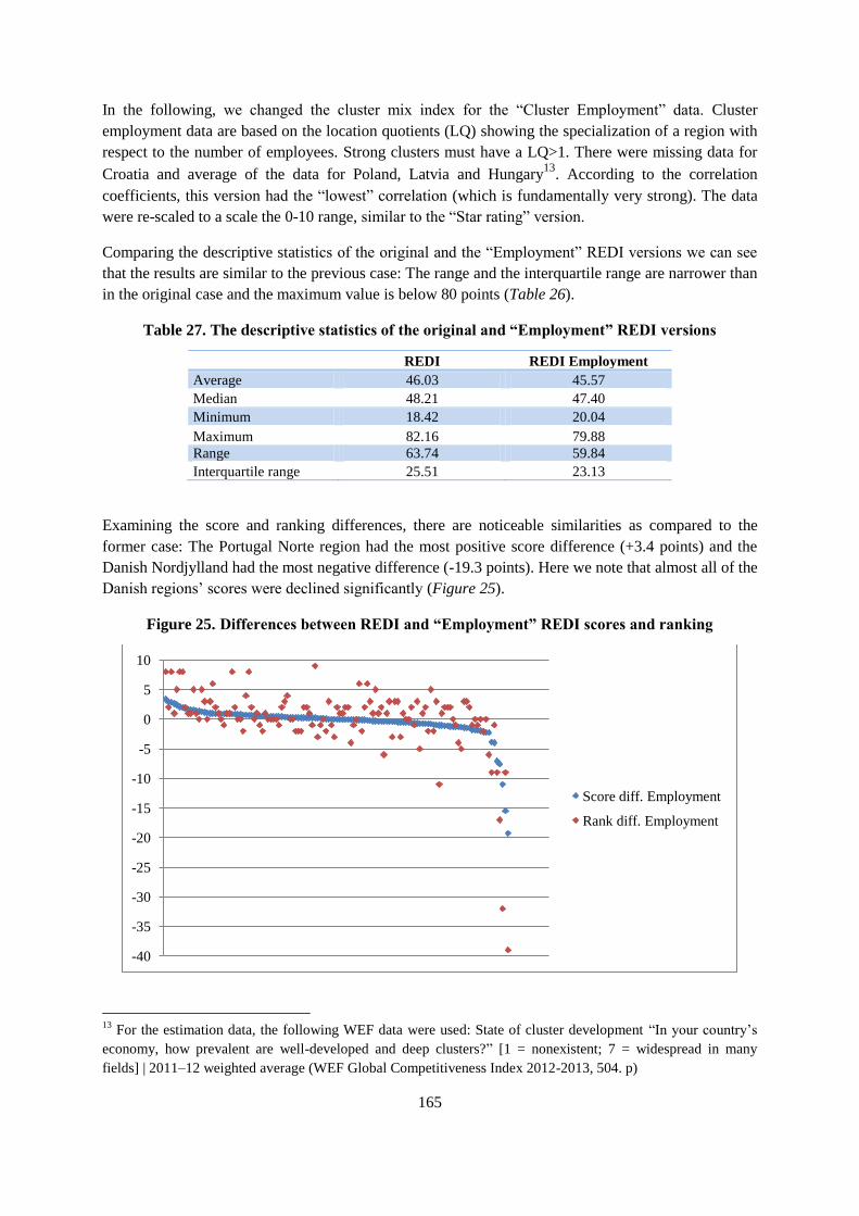
165
In the following, we changed the cluster mix index for the “Cluster Employment” data. Cluster
employment data are based on the location quotients (LQ) showing the specialization of a region with
respect to the number of employees. Strong clusters must have a LQ>1. There were missing data for
Croatia and average of the data for Poland, Latvia and Hungary13
. According to the correlation
coefficients, this version had the “lowest” correlation (which is fundamentally very strong). The data
were re-scaled to a scale the 0-10 range, similar to the “Star rating” version.
Comparing the descriptive statistics of the original and the “Employment” REDI versions we can see
that the results are similar to the previous case: The range and the interquartile range are narrower than
in the original case and the maximum value is below 80 points (Table 26).
Table 27. The descriptive statistics of the original and “Employment” REDI versions
REDI REDI Employment
Average 46.03 45.57
Median 48.21 47.40
Minimum 18.42 20.04
Maximum 82.16 79.88
Range 63.74 59.84
Interquartile range 25.51 23.13
Examining the score and ranking differences, there are noticeable similarities as compared to the
former case: The Portugal Norte region had the most positive score difference (+3.4 points) and the
Danish Nordjylland had the most negative difference (-19.3 points). Here we note that almost all of the
Danish regions’ scores were declined significantly (Figure 25).
Figure 25. Differences between REDI and “Employment” REDI scores and ranking
13
For the estimation data, the following WEF data were used: State of cluster development “In your country’s
economy, how prevalent are well-developed and deep clusters?” [1 = nonexistent; 7 = widespread in many
fields] | 2011–12 weighted average (WEF Global Competitiveness Index 2012-2013, 504. p)
-40
-35
-30
-25
-20
-15
-10
-5
0
5
10
Score diff. Employment
Rank diff. Employment

166
The Swedish Norra Mellansverige gained the most by 9 places (from 36th to 27
th) the Danish
Nordjylland fell by 39 places (from 8th to 47
th) in the ranking. As a consequence, London and French
Ile de France occupy the first two places in the “Employment” REDI ranking. The Danish
Hovedstaden, the former leader in most of the REDI rankings slipped down to the 10th place.
The next examined variable is “Cultural Support”. We investigated the effect of the modification of
two variables. First, we changed the original variable to “Corruption”. The Corruption data were based
on a standardized variable combining education (EdCor: region's aggregated score from survey
question on the extent to which corruption persists in the education system in the region/area), health
(HelCor: region's aggregated score from survey question on the extent to which corruption persists in
the health care system in the region/area), general public corruption (OtherCor: region's aggregated
score from survey question on the extent to which respondents felt other citizens in the region/area use
bribery to obtain public services), law enforcement (LawCor: region's aggregated score from survey
question on the extent to which corruption persists in the law enforcement in the region/area) and the
payment of bribes (HelBribe: region's aggregated score from survey question asking whether the
respondents were forced to pay a bribe in the last 12 months to obtain any health care in the
region/area)14
. Data are from 2009-2010 and they were re-scaled to a scale of 0 to 10.
We compared the main descriptive statistics values and we can see minimal differences (Table 27).
Out of the four examined versions the “Corruption” version shows the highest correlation with the
original version. However, it does not necessary mean that the ranking is also the same.
Table 28. The descriptive statistics of the original and “Corruption” REDI versions
REDI REDI Corruption
Average 46.03 46.69
Median 48.21 48.44
Minimum 18.42 18.66
Maximum 82.16 82.57
Range 63.74 63.72
Interquartile range 25.51 25.29
Based on Table 27, the Baltic states had the highest score difference: Estonia gained +2.1 points,
Latvia did +2 points and Lithuania did +1.8 points. The Belgian Région Wallone had the lowest score
difference with -0.6 points. Only five regions had their score difference below 0 meaning that score
differences disperse in a very narrow range (Figure 26).
14
Source: Nicholas Charron, Lewis Dijkstra & Victor Lapuente (2013): Regional Governance Matters: Quality
of Government within European Union Member States, Regional Studies, DOI:10.1080/00343404.2013.770141.
To link to this article: http://www.qog.pol.gu.se/digitalAssets/1446/1446579_regional-studies-article.pdf (9
August 2013).
Detailed description of the variable is available at: http://www.qog.pol.gu.se/digitalAssets/1362/1362471_eqi---
correlates-codebook.pdf (9 August 2013)
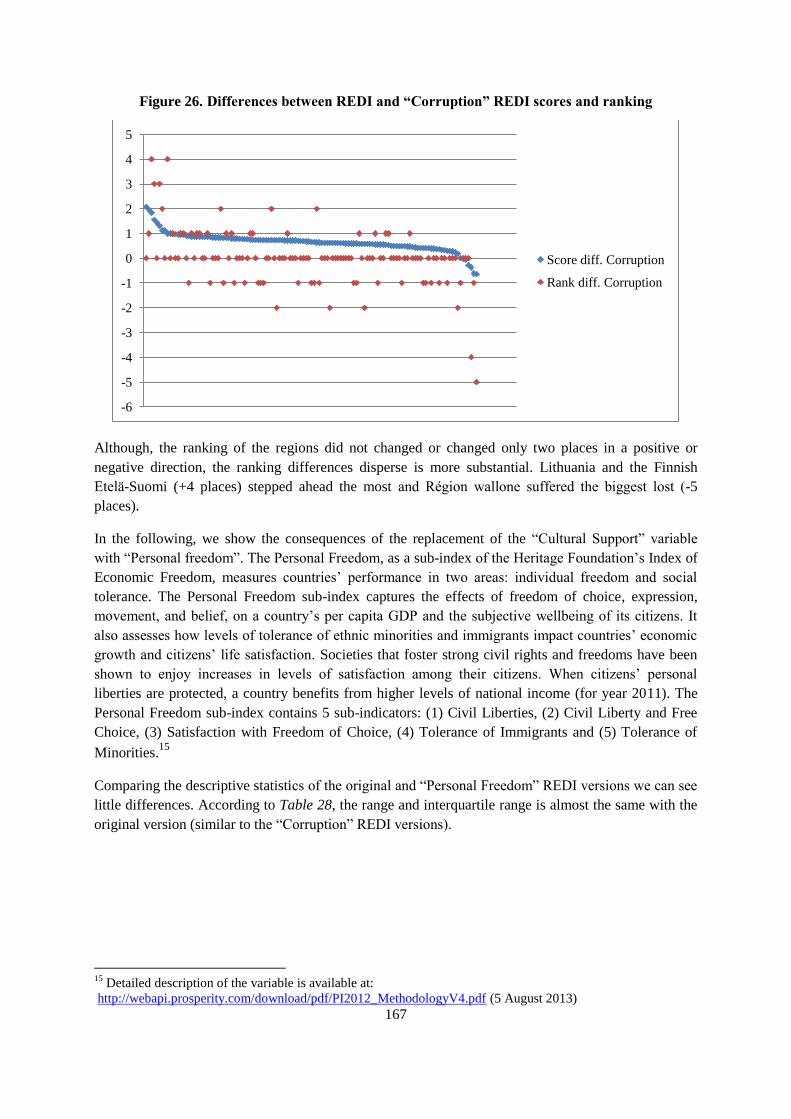
167
Figure 26. Differences between REDI and “Corruption” REDI scores and ranking
Although, the ranking of the regions did not changed or changed only two places in a positive or
negative direction, the ranking differences disperse is more substantial. Lithuania and the Finnish
Etelä-Suomi (+4 places) stepped ahead the most and Région wallone suffered the biggest lost (-5
places).
In the following, we show the consequences of the replacement of the “Cultural Support” variable
with “Personal freedom”. The Personal Freedom, as a sub-index of the Heritage Foundation’s Index of
Economic Freedom, measures countries’ performance in two areas: individual freedom and social
tolerance. The Personal Freedom sub-index captures the effects of freedom of choice, expression,
movement, and belief, on a country’s per capita GDP and the subjective wellbeing of its citizens. It
also assesses how levels of tolerance of ethnic minorities and immigrants impact countries’ economic
growth and citizens’ life satisfaction. Societies that foster strong civil rights and freedoms have been
shown to enjoy increases in levels of satisfaction among their citizens. When citizens’ personal
liberties are protected, a country benefits from higher levels of national income (for year 2011). The
Personal Freedom sub-index contains 5 sub-indicators: (1) Civil Liberties, (2) Civil Liberty and Free
Choice, (3) Satisfaction with Freedom of Choice, (4) Tolerance of Immigrants and (5) Tolerance of
Minorities.15
Comparing the descriptive statistics of the original and “Personal Freedom” REDI versions we can see
little differences. According to Table 28, the range and interquartile range is almost the same with the
original version (similar to the “Corruption” REDI versions).
15
Detailed description of the variable is available at:
http://webapi.prosperity.com/download/pdf/PI2012_MethodologyV4.pdf (5 August 2013)
-6
-5
-4
-3
-2
-1
0
1
2
3
4
5
Score diff. Corruption
Rank diff. Corruption

168
Table 29. The descriptive statistics of the original and “Personal Freedom” REDI versions
REDI REDI Personal Freedom
Average 46.03 47.74
Median 48.21 49.23
Minimum 18.42 20.17
Maximum 82.16 83.22
Range 63.74 63.05
Interquartile range 25.51 25.68
The highest difference of the scores between the old and the new version was +5.2 points (the
Slovakian Bratislavsky kraj) and the lowest (or highest negative) difference was noticed in the case of
Estonia with -4.3 points. Most of the score differences are above 0. There are only eight regions that
had a negative score difference. According the new version, the “winner” of the ranking was the
French Sud-Ouest, the Portugal Norte and the Hungarian Közép-Magyarország. Each region gained 6
places. The Belgian Région wallone suffered the biggest lost in ranking by 15 places. We note that all
of the Belgian regions slipped down significantly (Figure 27).
Figure 27. Differences between REDI and “Personal Freedom” REDI scores and ranking
The REDI points and the ranking of all the 125 regions with the original and four examined versions
can be found in Table 29.
-15
-12,5
-10
-7,5
-5
-2,5
0
2,5
5
7,5
Score diff. Freedom
Rank diff. Freedom
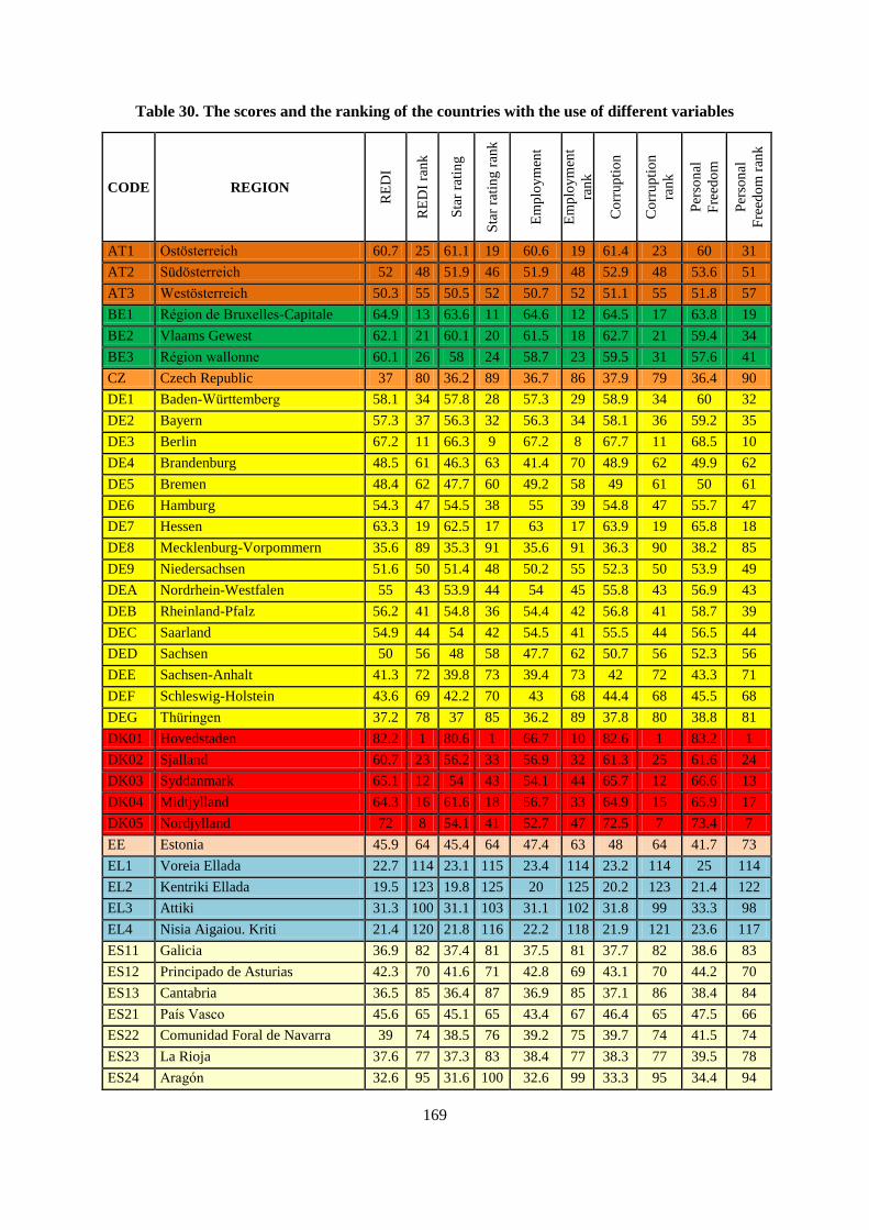
169
Table 30. The scores and the ranking of the countries with the use of different variables
CODE REGION
RE
DI
RE
DI
ran
k
Sta
r ra
tin
g
Sta
r ra
tin
g r
ank
Em
plo
ym
ent
Em
plo
ym
ent
ran
k
Co
rru
pti
on
Co
rru
pti
on
ran
k
Per
son
al
Fre
edo
m
Per
son
al
Fre
edo
m r
ank
AT1 Ostösterreich 60.7 25 61.1 19 60.6 19 61.4 23 60 31
AT2 Südösterreich 52 48 51.9 46 51.9 48 52.9 48 53.6 51
AT3 Westösterreich 50.3 55 50.5 52 50.7 52 51.1 55 51.8 57
BE1 Région de Bruxelles-Capitale 64.9 13 63.6 11 64.6 12 64.5 17 63.8 19
BE2 Vlaams Gewest 62.1 21 60.1 20 61.5 18 62.7 21 59.4 34
BE3 Région wallonne 60.1 26 58 24 58.7 23 59.5 31 57.6 41
CZ Czech Republic 37 80 36.2 89 36.7 86 37.9 79 36.4 90
DE1 Baden-Württemberg 58.1 34 57.8 28 57.3 29 58.9 34 60 32
DE2 Bayern 57.3 37 56.3 32 56.3 34 58.1 36 59.2 35
DE3 Berlin 67.2 11 66.3 9 67.2 8 67.7 11 68.5 10
DE4 Brandenburg 48.5 61 46.3 63 41.4 70 48.9 62 49.9 62
DE5 Bremen 48.4 62 47.7 60 49.2 58 49 61 50 61
DE6 Hamburg 54.3 47 54.5 38 55 39 54.8 47 55.7 47
DE7 Hessen 63.3 19 62.5 17 63 17 63.9 19 65.8 18
DE8 Mecklenburg-Vorpommern 35.6 89 35.3 91 35.6 91 36.3 90 38.2 85
DE9 Niedersachsen 51.6 50 51.4 48 50.2 55 52.3 50 53.9 49
DEA Nordrhein-Westfalen 55 43 53.9 44 54 45 55.8 43 56.9 43
DEB Rheinland-Pfalz 56.2 41 54.8 36 54.4 42 56.8 41 58.7 39
DEC Saarland 54.9 44 54 42 54.5 41 55.5 44 56.5 44
DED Sachsen 50 56 48 58 47.7 62 50.7 56 52.3 56
DEE Sachsen-Anhalt 41.3 72 39.8 73 39.4 73 42 72 43.3 71
DEF Schleswig-Holstein 43.6 69 42.2 70 43 68 44.4 68 45.5 68
DEG Thüringen 37.2 78 37 85 36.2 89 37.8 80 38.8 81
DK01 Hovedstaden 82.2 1 80.6 1 66.7 10 82.6 1 83.2 1
DK02 Sjalland 60.7 23 56.2 33 56.9 32 61.3 25 61.6 24
DK03 Syddanmark 65.1 12 54 43 54.1 44 65.7 12 66.6 13
DK04 Midtjylland 64.3 16 61.6 18 56.7 33 64.9 15 65.9 17
DK05 Nordjylland 72 8 54.1 41 52.7 47 72.5 7 73.4 7
EE Estonia 45.9 64 45.4 64 47.4 63 48 64 41.7 73
EL1 Voreia Ellada 22.7 114 23.1 115 23.4 114 23.2 114 25 114
EL2 Kentriki Ellada 19.5 123 19.8 125 20 125 20.2 123 21.4 122
EL3 Attiki 31.3 100 31.1 103 31.1 102 31.8 99 33.3 98
EL4 Nisia Aigaiou. Kriti 21.4 120 21.8 116 22.2 118 21.9 121 23.6 117
ES11 Galicia 36.9 82 37.4 81 37.5 81 37.7 82 38.6 83
ES12 Principado de Asturias 42.3 70 41.6 71 42.8 69 43.1 70 44.2 70
ES13 Cantabria 36.5 85 36.4 87 36.9 85 37.1 86 38.4 84
ES21 País Vasco 45.6 65 45.1 65 43.4 67 46.4 65 47.5 66
ES22 Comunidad Foral de Navarra 39 74 38.5 76 39.2 75 39.7 74 41.5 74
ES23 La Rioja 37.6 77 37.3 83 38.4 77 38.3 77 39.5 78
ES24 Aragón 32.6 95 31.6 100 32.6 99 33.3 95 34.4 94
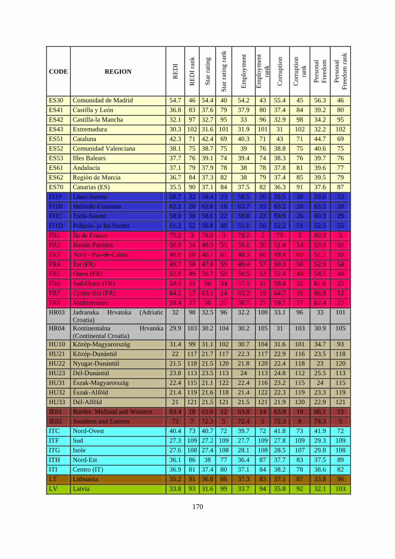
170
CODE REGION
RE
DI
RE
DI
ran
k
Sta
r ra
tin
g
Sta
r ra
tin
g r
ank
Em
plo
ym
ent
Em
plo
ym
ent
ran
k
Co
rru
pti
on
Co
rru
pti
on
ran
k
Per
son
al
Fre
edo
m
Per
son
al
Fre
edo
m r
ank
ES30 Comunidad de Madrid 54.7 46 54.4 40 54.2 43 55.4 45 56.3 46
ES41 Castilla y León 36.8 83 37.6 79 37.9 80 37.4 84 39.2 80
ES42 Castilla-la Mancha 32.1 97 32.7 95 33 96 32.9 98 34.2 95
ES43 Extremadura 30.3 102 31.6 101 31.9 101 31 102 32.2 102
ES51 Cataluna 42.3 71 42.4 69 40.3 71 43 71 44.7 69
ES52 Comunidad Valenciana 38.1 75 38.7 75 39 76 38.8 75 40.6 75
ES53 Illes Balears 37.7 76 39.1 74 39.4 74 38.3 76 39.7 76
ES61 Andalucía 37.1 79 37.9 78 38 78 37.8 81 39.6 77
ES62 Región de Murcia 36.7 84 37.3 82 38 79 37.4 85 39.5 79
ES70 Canarias (ES) 35.5 90 37.1 84 37.5 82 36.3 91 37.6 87
FI19 Länsi-Suomi 58.7 32 58.4 23 58.5 26 59.5 30 59.6 33
FI1B Helsinki-Uusimaa 62.2 20 62.8 16 63.7 15 63.2 20 63.5 20
FI1C Etelä-Suomi 58.9 30 58.6 22 59.8 22 59.9 26 60.3 29
FI1D Pohjois- ja Ita-Suomi 51.2 52 50.8 49 51.1 50 52.2 51 52.5 55
FR1 Île de France 79.2 3 78.9 3 79.2 2 79 3 80.9 3
FR2 Bassin Parisien 50.9 54 48.9 55 50.1 56 51.4 54 53.6 50
FR3 Nord - Pas-de-Calais 48.8 60 46.7 61 48.3 60 49.4 60 51.5 59
FR4 Est (FR) 49.7 58 47.8 59 49.4 57 50.3 58 52.9 54
FR5 Ouest (FR) 51.8 49 50.7 50 50.5 53 52.4 49 54.5 48
FR6 Sud-Ouest (FR) 58.9 31 56 34 57.1 31 59.4 32 61.6 25
FR7 Centre-Est (FR) 64.2 17 63.1 14 63.2 16 64.7 16 66.8 12
FR8 Méditerranée 59.4 27 58 25 58.7 25 59.7 27 62.4 22
HR03 Jadranska Hrvatska (Adriatic
Croatia)
32 98 32.5 96 32.2 100 33.1 96 33 101
HR04 Kontinentalna Hrvatska
(Continental Croatia)
29.9 103 30.2 104 30.2 105 31 103 30.9 105
HU10 Közép-Magyarország 31.4 99 31.1 102 30.7 104 31.6 101 34.7 93
HU21 Közép-Dunántúl 22 117 21.7 117 22.3 117 22.9 116 23.5 118
HU22 Nyugat-Dunántúl 21.5 118 21.5 120 21.8 120 22.4 118 23 120
HU23 Dél-Dunántúl 23.8 113 23.5 113 24 113 24.8 112 25.5 113
HU31 Észak-Magyarország 22.4 115 21.1 122 22.4 116 23.2 115 24 115
HU32 Észak-Alföld 21.4 119 21.6 118 21.4 122 22.3 119 23.3 119
HU33 Dél-Alföld 21 121 21.5 121 21.5 121 21.9 120 22.9 121
IE01 Border. Midland and Western 63.4 18 63.6 12 63.8 14 63.9 18 66.1 15
IE02 Southern and Eastern 72 7 72.3 5 72.4 5 72.3 8 74.3 5
ITC Nord-Ovest 40.4 73 40.7 72 39.7 72 41.8 73 41.9 72
ITF Sud 27.3 109 27.2 109 27.7 109 27.8 109 29.3 109
ITG Isole 27.6 108 27.4 108 28.1 108 28.5 107 29.8 108
ITH Nord-Est 36.1 86 38 77 36.4 87 37.7 83 37.5 89
ITI Centro (IT) 36.9 81 37.4 80 37.1 84 38.2 78 38.6 82
LT Lithuania 35.2 91 36.8 86 37.3 83 37.1 87 33.8 96
LV Latvia 33.8 93 31.6 99 33.7 94 35.8 92 32.1 103
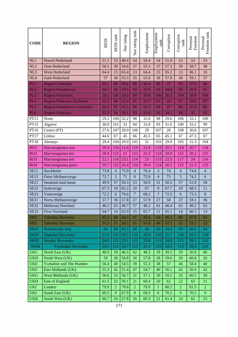
171
CODE REGION
RE
DI
RE
DI
ran
k
Sta
r ra
tin
g
Sta
r ra
tin
g r
ank
Em
plo
ym
ent
Em
plo
ym
ent
ran
k
Co
rru
pti
on
Co
rru
pti
on
ran
k
Per
son
al
Fre
edo
m
Per
son
al
Fre
edo
m r
ank
NL1 Noord-Nederland 51.1 53 49.4 54 50.4 54 51.8 53 53 53
NL2 Oost-Nederland 56.5 39 54.6 37 55.3 37 57.3 39 58.7 38
NL3 West-Nederland 64.4 15 63.4 13 64.4 13 65.1 13 66.1 16
NL4 Zuid-Nederland 57 38 55.5 35 55.6 36 57.8 38 59.1 37
PL1 Region Centralny 36.1 88 36.4 88 36.4 88 37 89 37.6 88
PL2 Region Poludniowy 34.1 92 33.5 92 33.6 95 34.8 93 35.9 91
PL3 Region Wschodni 29.2 105 28.5 107 29.8 106 30.2 104 30.9 106
PL4 Region Pólnocno-Zachodni 32.3 96 32.4 97 32.7 97 33 97 33.8 97
PL5 Region Poludniowo-Zachodni 36.1 87 35.3 90 35.7 90 37 88 37.8 86
PL6 Region Pólnocny 33.2 94 33.1 93 33.8 92 34.1 94 35 92
PT11 Norte 29.2 106 32.2 98 32.6 98 29.6 106 33.1 100
PT15 Algarve 30.9 101 33 94 33.8 93 31.6 100 33.2 99
PT16 Centro (PT) 27.6 107 28.9 106 29 107 28 108 30.8 107
PT17 Lisboa 44.6 67 45 66 45.5 65 45.1 67 47.5 67
PT18 Alentejo 29.4 104 29.9 105 31 103 29.9 105 31.3 104
RO1 Macroregiunea unu 19.4 124 21.6 119 21.8 119 20.1 124 20.7 124
RO2 Macroregiunea doi 18.4 125 21 123 21.3 123 18.9 125 20.2 125
RO3 Macroregiunea trei 22.1 116 23.1 114 23 115 22.5 117 24 116
RO4 Macroregiunea patru 19.7 122 20.4 124 20.4 124 20.2 122 21.3 123
SE11 Stockholm 73.8 4 75.9 4 76.4 3 74 4 74.8 4
SE12 Östra Mellansverige 72.7 5 71 6 72.9 4 73 5 74.2 6
SE21 Smaland med öarna 49.9 57 50.3 53 50.9 51 50.5 57 51.8 58
SE22 Sydsverige 67.3 10 65.2 10 67 9 67.7 10 68.5 11
SE23 Vastsverige 72.2 6 70.6 7 68.2 7 72.5 6 73.3 8
SE31 Norra Mellansverige 57.7 36 57.8 27 57.9 27 58 37 59.1 36
SE32 Mellersta Norrland 48.2 63 48.7 57 48.2 61 48.4 63 49.2 63
SE33 Övre Norrland 64.7 14 62.9 15 65.7 11 65.1 14 66.5 14
SI01 Vzhodna Slovenija 45.3 66 44.5 67 45.6 64 46.3 66 47.6 65
SI02 Zahodna Slovenija 51.3 51 50.5 51 51.6 49 52.1 52 53.1 52
SK01 Bratislavsky kraj 44 68 43.3 68 44 66 43.4 69 49.2 64
SK02 Západné Slovensko 25.8 110 26.5 110 26.9 110 25.7 110 29.3 110
SK03 Stredné Slovensko 24.9 111 25.1 111 25.8 111 24.9 111 28.1 112
SK04 Vychodné Slovensko 24.5 112 24.7 112 25.3 112 24.5 113 28.4 111
UKC North East (UK) 48.9 59 46.5 62 48.3 59 49.5 59 50.8 60
UKD North West (UK) 59 28 56.8 30 57.8 28 59.6 29 60.8 26
UKE Yorkshire and The Humber 56.4 40 54.5 39 55.3 38 57 40 58.4 40
UKF East Midlands (UK) 55.3 42 51.4 47 54.7 40 56.1 42 56.9 42
UKG West Midlands (UK) 58.6 33 56.7 31 57.1 30 59.2 33 60.5 28
UKH East of England 61.5 22 59.1 21 60.4 20 62 22 63 21
UKI London 79.9 2 79.6 2 79.9 1 80.2 2 81.5 2
UKJ South East (UK) 69.5 9 67.9 8 69.3 6 70.1 9 70.5 9
UKK South West (UK) 60.7 24 57.8 26 60.3 21 61.4 24 62 23

172
CODE REGION
RE
DI
RE
DI
ran
k
Sta
r ra
tin
g
Sta
r ra
tin
g r
ank
Em
plo
ym
ent
Em
plo
ym
ent
ran
k
Co
rru
pti
on
Co
rru
pti
on
ran
k
Per
son
al
Fre
edo
m
Per
son
al
Fre
edo
m r
ank
UKL Wales 54.7 45 48.7 56 53.4 46 55.3 46 56.3 45
UKM Scotland 59 29 57.7 29 58.7 24 59.7 28 60.5 27
UKN Northern Ireland (UK) 58 35 52.9 45 55.8 35 58.8 35 60.1 30

KN-02-14-462-EN
-N


![Index [smartabhyas.com]smartabhyas.com/asset/images/docs/14ccfb99ce7cf04e9e70f98ada… · Index 1. Women Entrepreneurship Centre to come up…………………………………………………….01](https://cdn.vdocuments.mx/doc/165x107/5e9b1c9e84903042155e121d/index-index-1-women-entrepreneurship-centre-to-come-up01-2-border-development.jpg)
