
1
Recent Advances in Mathematical Programming Techniques for the Optimization of Process Systems under Uncertainty
Ignacio E. GrossmannRobert M. Apap, Bruno A. Calfa, Pablo Garcia-Herreros, Qi Zhang
Center for Advanced Process Decision-makingDepartment of Chemical Engineering
Carnegie Mellon UniversityPittsburgh, PA 15213, U.S.A.
Presented at PSE2015-ESCAPE 2531 May - 4 June 2015
Copenhagen, Denmark
EWO Seminar, September 15, 2015

2
Motivation Optimization under UncertaintyOptimization models for synthesis, design, planning, scheduling and control often involve uncertainties (parameters)
Design/SynthesisQuality feedstocksKinetic constantsTransfer coefficients
Supply Chain/PlanningProduct demandsPrices productsYields
Basic questions: How to model problems with uncertainty?How to solve them effectively?How to account for historical data/forecasts?

3
History in Process Systems Engineering
Optimal Design under Uncertainty (Stochastic Programming)Takamatsu, Hashimoto, Shioya (1973)Dittmar and Hartmann (1976)Johns, Marketos, Rippin (1976)Grossmann and Sargent (1978)
Planning under Uncertainty (Stochastic Programming)Liu, Sahinidis (1996)Acevedo, Pistikopoulos (1998)Gupta, Maranas (2000)Applequist, Pekny, Reklaitis(2000)
Robust OptimizationFriedman, Rekalitis (1975)Swaney, Grossmann (1985)Lin, SL Janak, CA Floudas (2004)
Chance constrainedArellano-Garcia, Martini, Wendt, Li, Wozny (2003)
Sample papers

4
Stage 1Here & now
RecourseWait & seeu
u1
u2
If deterministic uncertainty set
Robust Optimization: Ensure feasibility over uncertainty set
Approaches to Optimization under Uncertainty Sahinidis (2004)
How to anticipate effects of uncertainty?
If probability distribution functionStochastic Programming: Expected value, recourse actions
Chance Constrained Optimization: Ensure feasibility level confidence
Impact of optimization under uncertaintyhas been limited in industrial practice
Major reasons: ill-defined problem, computational expense
Option: add risk measure
u1
u2
U

5
Several major challenges and barriers:
1. How to avoid overly conservative results in robust optimization?
2. How to effectively solve two- or multi-stage stochastic optimization problems?
3. How to handle complexity of exogenous and endogenous uncertainties in multi-stage stochastic programming?
4. How to incorporate historical data in the generation of scenarios?
Presentation restricted to LP/MILP models

6
Remove uncertain parametersin the objective:
Robust Optimization
Ben-Tal et al. (2009); Bertsimas and Sim (2003)
Major concern: feasibility over uncertainty set
Uncertainty set
LP:
UumibxuAst
xcT
x
,...1)(
min
Uncertainty sets
u1
u2
u1
u2
Semi-infinite programming problem

7
Scheduling: Lin, Janak, Floudas (2004)Bertsimas, Thiele (2006)Li, Ierapetritou (2008)Verderame, Floudas (2010)Vujanic et al. (2012)
Supply Chain:Bertsimas, Sim (2003)Bertsimas, Thiele (2004)Hahn, Kuhn (2012)Gounaris, Wiesemann, Floudas (2013)
Process Synthesis:Tay, Ng, Tan (2013)Kasivisvanathan et al. (2014)
Previous Work Robust Optimization
8
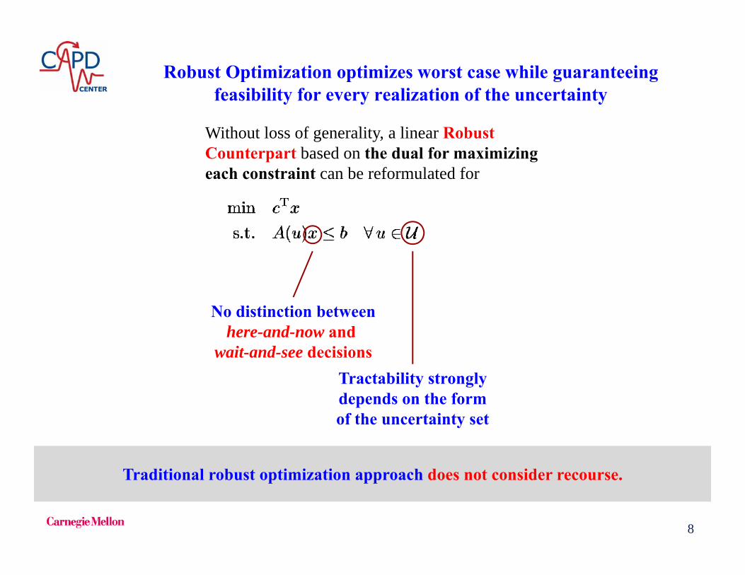
Robust Optimization optimizes worst case while guaranteeing feasibility for every realization of the uncertainty
Without loss of generality, a linear RobustCounterpart based on the dual for maximizingeach constraint can be reformulated for
No distinction betweenhere-and-now and
wait-and-see decisionsTractability stronglydepends on the formof the uncertainty set
Traditional robust optimization approach does not consider recourse.

9
Recourse: Decision rules are optimized with respect to uncertain parameters
Consider the following “two-stage” robust optimization problem:
1st stage 2nd stage
Instead of fixing the 2nd-stage decision variables, consider them to befunctions of the uncertain parameters. → Adjustable Robust Counterpart (ARC)
Recourse since reactive actions dependon the realization of the uncertainty
Ben-Tal et al. (2004). Math Programming.

10
Tractable reformulations can be obtained for the Adjustable Robust Counterpart in certain cases
1. Polyhedral or, more generally, conic uncertainty set:
2. Affine decision rules:
Dependence of parameters:
3. Fixed recourse( independent of ):
nominal values deviation
Affinely Adjustable Robust Counterpart (AARC)Ben-Tal et al. (2004). Math Programming.
where is a convex cone with dual .
11
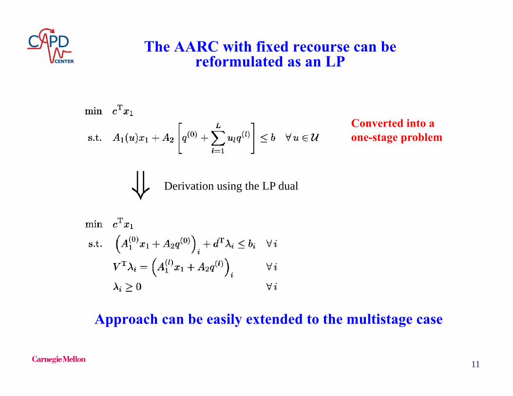
The AARC with fixed recourse can bereformulated as an LP
Derivation using the LP dual
Converted into aone-stage problem
Approach can be easily extended to the multistage case
12
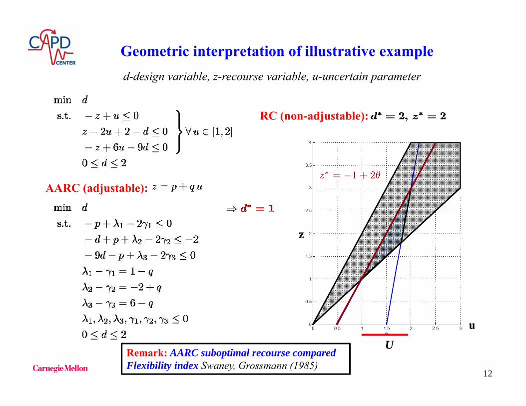
Geometric interpretation of illustrative example
RC (non-adjustable):
AARC (adjustable):
Remark: AARC suboptimal recourse comparedFlexibility index Swaney, Grossmann (1985)
z
u
d-design variable, z-recourse variable, u-uncertain parameter
U

13
Industrial case study: Integrated Air Separation Unit (ASU)-Cryogenic Energy Storage (CES) participates in two electricity markets*
Liquid inventory
Driox
Gas demand
Liquid demand
CES inventory
Electricity generation
Electricenergy market
ASU
Operating reserve market
LO2, LN2, LAr
LO2, LN2
GO2, GN2Vented gas
Sold electricity
Provided reserve
Purchased electricity
For internal use
Air
Purchasedliquid
LO2, LN2
Uncertainty in reserve demand
Zhang, Heuberger, Grossmann, Pinto, Sundramoorthy (2015)

14
AARC formulation ensures feasible schedule makingthe provision of operating reserve capacity possible.
• Multistage formulation: first stage: base plant operation, reserve capacity• recourse: liquid produced (linear with reserve demand)• Large-scale MILP: 53,000 constraints, 55,000 continuous variables, 2,500 binaries
CPLEX 12.5 , 10 min CPU-time (1% gap)
-0.1
-0.05
0
0.05
0.1
0
0.2
0.4
0.6
0.8
0 12 24 36 48 60 72 84 96 108 120 132 144 156 168
In a
nd O
ut F
low
s
CE
S In
vent
ory
Time [h] Liquid Flow into CES Tank Converted to Power for Internal Use Converted to Power to be Sold Committed Reserve Capacity CES Inventory Spinning Reserve Price Electricity Price
-0.1
-0.05
0
0.05
0.1
0
0.2
0.4
0.6
0.8
0 12 24 36 48 60 72 84 96 108 120 132 144 156 168
In a
nd O
ut F
low
s
CE
S In
vent
ory
Time [h]
-0.1
-0.05
0
0.05
0.1
0
0.2
0.4
0.6
0.8
0 12 24 36 48 60 72 84 96 108 120 132 144 156 168
In a
nd O
ut F
low
s
CE
S In
vent
ory
Time [h]
-0.1
-0.05
0
0.05
0.1
0
0.2
0.4
0.6
0.8
0 12 24 36 48 60 72 84 96 108 120 132 144 156 168
In a
nd O
ut F
low
s
CE
S In
vent
ory
Time [h]
-0.1
-0.05
0
0.05
0.1
0
0.2
0.4
0.6
0.8
0 12 24 36 48 60 72 84 96 108 120 132 144 156 168
In a
nd O
ut F
low
s
CE
S In
vent
ory
Time [h]
CES inventory profile plotted for the case of no dispatch

15
0
0.5
1
0.67 0.81 0.84
Prob
abili
ty
Uncertain Parameter Value
Stochastic programming is a scenario-based framework for optimization under uncertainty (Birge & Louveaux, 2011)
LM
H
0 1 2 Time horizon is divided into a set of
discrete time points
Uncertain parameters are described by adiscretized probability distribution
Stochastic Programming
Discretized distribution gives rise to Scenario Tree
L M H
u1 u2 u3

16
min )]...]()([...)()([ 222112
NNNuu uxucEuxucExcz N
s.t. 111 hxW
)()()( 222211 uhuxWxuT
)()()()( 111 uhuxWuxuT NNNNNNN
1,...,2,0)(,01 Ntuxx tt
…
Multistage Stochastic Programming
Special case: two-stage programming (N=2)
Birge & Louveaux, 1997; Sahinidis, 2004
Exogeneous uncertainties(e.g. demands)
x1 stage 1 u x2 recourse (stage 2)
u
17
Process Design/Synthesis:Halemane, Grossmann (1983)Pistikopoulos, Ierapetritou (1995)Cheng, Subrahmanian, Westerberg (2003)Pintarič, Kravanja (2003)
Supply Chain:Tsiakis, Shah, Pantelides (2001)Jung, Blau, Pekny, Reklaitis, Eversdyk (2004)You, Wassick, Grossmann (2009)Baptista, Gomes, Barbosa-Povoa (2012)
SchedulingSand, Engell (2004)
Methodology: Magnanti, Wong (1981)Birge, Louveaux (1988)Caroe, Schultz (1999)Sahiridis, Minoux, Ierapetritou (2010)
Previous Work Two-Stage Programming

18
Decomposition Techniques
18
A
D1
D3
D2
Complicating Constraints
max
1,..{ , 1,.. , 0}
T
i i i
i i
c xst Ax b
D x d i nx X x x i n x
x1 x2 x3
Lagrangean decompositionGeoffrion (1972) Guinard (2003)
complicatingconstraints
D1
D3
D2
Complicating Variables
A
x1 x2 x3y
1,..max
1,..0, 0, 1,..
T Ti i
i n
i i i
i
a y c x
st Ay D x d i ny x i n
complicatingvariables
Benders decompositionBenders (1962), Magnanti, Wong (1984)
Multistage Stochastic ProgrammingTwo-stage Stochastic Programming

19
Supply plant
Candidate locations for DCs with risk of major disruption earthquakes, fires, strikes
Customers with deterministic demands for multiple commodities
Scenarios given by the combination of disruptions
Selecting DCs among candidate locations
Determining storage capacity in selected DCs
Allocating demands in every scenario
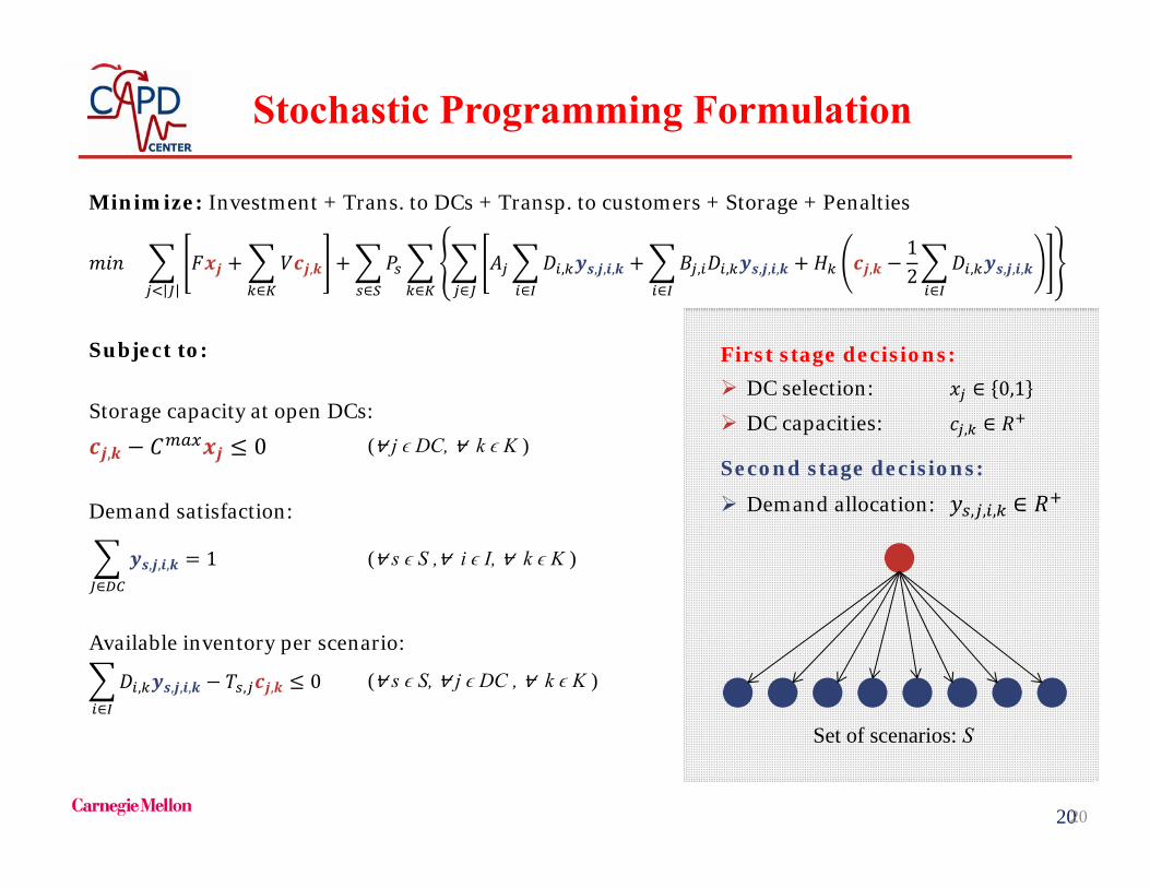
Supply Chain Design with Risk of Disruptions
Given:
Minimize cost by:
DCs=Distribution Centers
Garcia-Herreros, Wassick, Grossmann (2014)
2020
Minimize: Investment + Trans. to DCs + Transp. to customers + Storage + Penalties
,∈
, , , ,∈
, , , , ,∈
,12 , , , ,
∈∈∈∈
Subject to:
Storage capacity at open DCs:
, 0
Demand satisfaction:
, , ,∈
1
Available inventory per scenario:
, , , ,∈
, , 0
(⩝ s ϵ S ,⩝ i ϵ I, ⩝ k ϵ K )
(⩝ j ϵ DC, ⩝ k ϵ K )
(⩝ s ϵ S, ⩝ j ϵ DC , ⩝ k ϵ K )
Stochastic Programming Formulation
Set of scenarios: S
First stage decisions: DC selection: ∈ 0,1
DC capacities: , ∈
Second stage decisions:
Demand allocation: , , , ∈

21
(You & Grossmann, 2008)
Supply chain network: 1 production plant 3 candidate locations for DCs 6 customers 1 commodity
Deterministicformulation
Resilientformulation
Computationalstatistics
Problem type MILP MILPNo. of constraints 13 76No. of continuous variables 31 199No. of binary variables 3 3Solution time 0.058s 0.405s
Expectedcostsunderriskofdisruptions
Investment ($) 279,900 419,850Transportation to DCs ($) 70,098 68,971Transportation to customers ($) 59,029 54,683Storage ($) 1,593 2,927Penalties ($) 674,703 54,244Total ($): 1,085,323 600,675
Solution Storage capacity 298/‐ /501 400/400/400
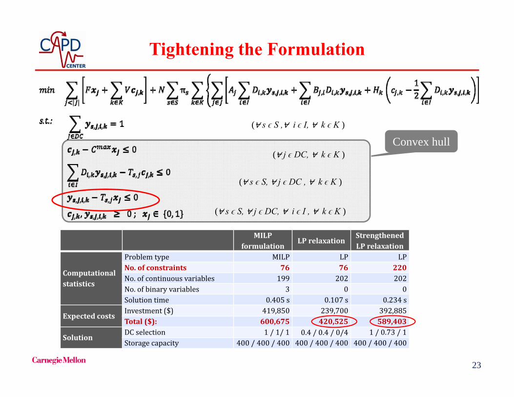
Illustrative Example

22
Challenges
Relaxation
Weak LP relaxation Time consuming for
Branch-and-bound
Scenarios’ probabilities
Different orders of magnitude among scenario probabilities
Number of scenarios
Exponential growth with number of candidate DCs
Approaches
Relaxation
Tightening constraints
Strengthen Benders master problem by including first scenario
Scenarios’ probabilities
Select the relevant subset of scenarios
Find deterministic bounds on the remaining scenarios
Number of scenarios
Solve a subset of scenarios Multicut Benders
decomposition
23
(⩝ s ϵ S ,⩝ i ϵ I, ⩝ k ϵ K )
(⩝ j ϵ DC, ⩝ k ϵ K )
(⩝ s ϵ S, ⩝ j ϵ DC , ⩝ k ϵ K )
(⩝ s ϵ S, ⩝ j ϵ DC, ⩝ i ϵ I , ⩝ k ϵ K )
Convex hull
MILPformulation
LPrelaxationStrengthenedLPrelaxation
Computationalstatistics
Problem type MILP LP LPNo. of constraints 76 76 220No. of continuous variables 199 202 202No. of binary variables 3 0 0Solution time 0.405s 0.107s 0.234s
ExpectedcostsInvestment ($) 419,850 239,700 392,885Total ($): 600,675 420,525 589,403
SolutionDC selection 1/1/1 0.4/0.4/0/4 1/0.73 /1Storage capacity 400/400/400 400/400/400 400/400/400
Tightening the Formulation

24
Reduction Number of Scenarios
- Sampling: ProbabilisticSampling Average Approximation (Shapiro & Homem-de-Mello (2000)
Predict probabilistic lower/upper bounds
- Scenario tree reduction: DeterministicOptimal scenario reduction (Heitsch, Roemisch, 2003; Li, Floudas, 2012))
Exclude scenarios within certain probability distance
- Reduction based on magnitude of probabilitiese.g. Supply chain disruptions
Probabilities of no disrupt > up to 1 > up to 2 > up to 3...

25
Assignment policyFind an upper bound by calculating the cost in the subset of neglected scenarios of a policy that is always feasible
Policy: attempt main-scenario assignments for all demands• If assignment is feasible (DC is active) => cost of main-scenario• If assignment is infeasible (DC is disrupted) => cost of penalty
The proportion in which assignments (y1,j,i,k) are feasible is given by the conditionalprobability of disruption at DC j ( ) in the subset of neglected scenarios ( )
Properties of scenarios generated from independent disruption probabilities
25
Bounds on Neglected Scenarios

26
Algorithmic Implementation Benders Decomposition
Subset Scenarios
Indistinguishable Scenarios
Multi-cuts
Pareto cuts
Parallel computation
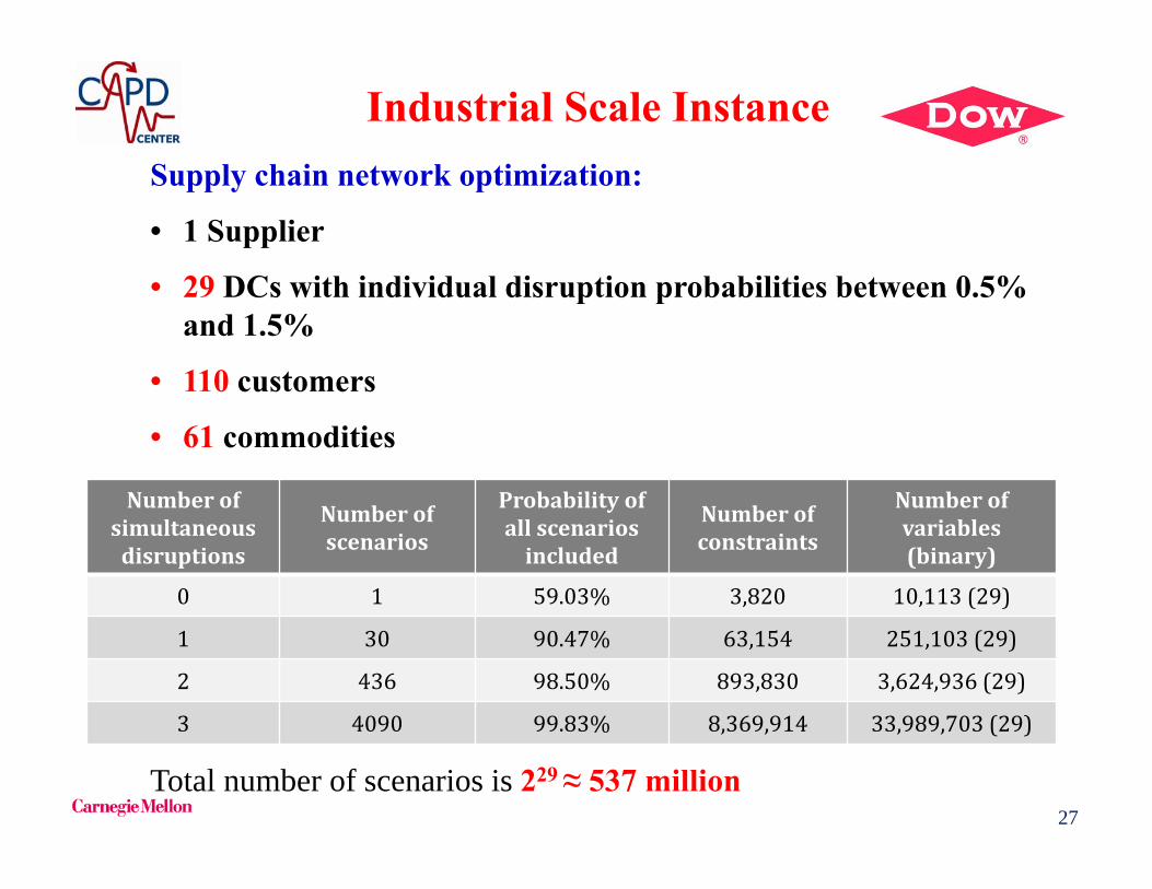
27
Industrial Scale InstanceSupply chain network optimization:
• 1 Supplier
• 29 DCs with individual disruption probabilities between 0.5% and 1.5%
• 110 customers
• 61 commodities
Total number of scenarios is 229 ≈ 537 million
Numberofsimultaneousdisruptions
Numberofscenarios
Probabilityofall scenariosincluded
Numberofconstraints
Numberofvariables(binary)
0 1 59.03% 3,820 10,113(29)
1 30 90.47% 63,154 251,103(29)
2 436 98.50% 893,830 3,624,936(29)
3 4090 99.83% 8,369,914 33,989,703(29)
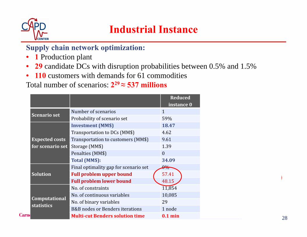
28
Supply chain network optimization:• 1 Production plant• 29 candidate DCs with disruption probabilities between 0.5% and 1.5%• 110 customers with demands for 61 commoditiesTotal number of scenarios: 229 ≈ 537 millions
28
Reducedinstance0
Reducedinstance1
Reducedinstance2
ScenariosetNumber of scenarios 1 30 436Probability of scenario set 59% 90.5% 98.5%
Expectedcostsforscenarioset
Investment (MM$) 18.47 18.77 21.56Transportation to DCs (MM$) 4.62 11.11 11.72Transportation to customers (MM$) 9.61 13.12 16.73Storage (MM$) 1.39 2.37 3.31Penalties (MM$) 0 3.31 0.54Total (MM$): 34.09 48.68 53.85
SolutionFinal optimality gap for scenario set 0% 0.78% 0.77%Full problem upper bound 57.41 56.31 55.10Full problem lower bound 48.15 52.87 53.87
Computationalstatistics
No. of constraints 11,854 304,261 4,397,989No. of continuous variables 10,085 251,191 3,626,675No. of binary variables 29 29 29B&B nodes or Benders iterations 1 node 4iterations 6iterationsMulti‐cut Benders solution time 0.1 min 84min 1762min
Industrial Instance
29
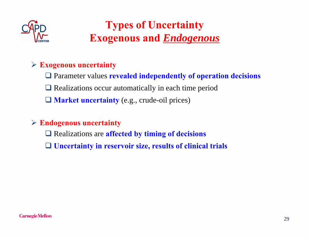
Types of UncertaintyExogenous and Endogenous
Exogenous uncertainty Parameter values revealed independently of operation decisions Realizations occur automatically in each time periodMarket uncertainty (e.g., crude-oil prices)
Endogenous uncertainty Realizations are affected by timing of decisions Uncertainty in reservoir size, results of clinical trials
30
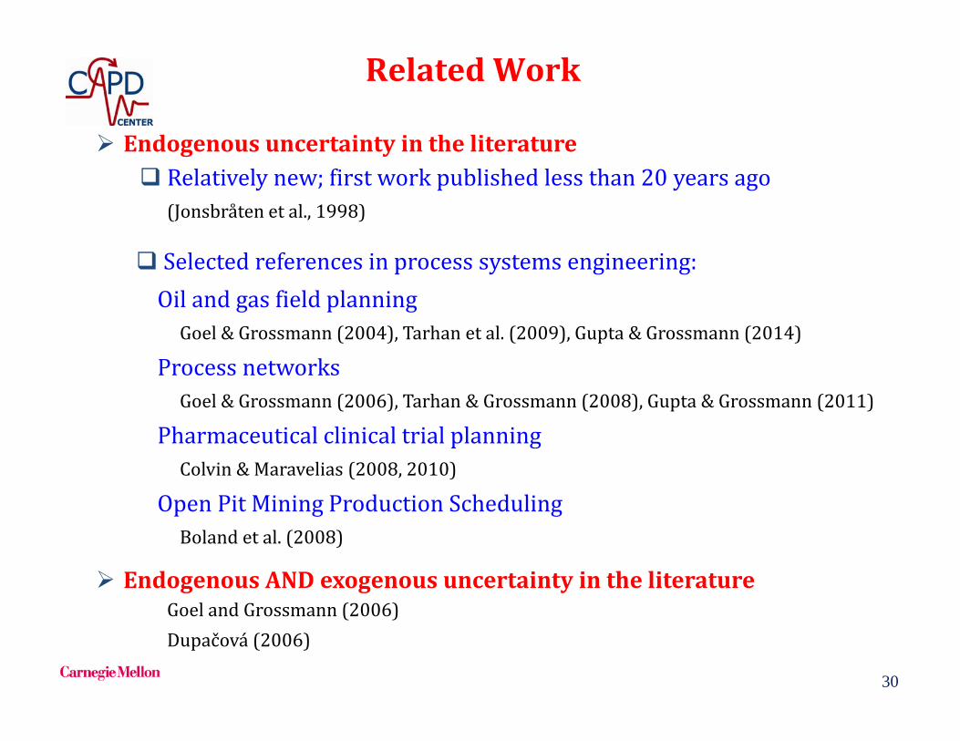
RelatedWork
Endogenousuncertaintyintheliterature Relativelynew;firstworkpublishedlessthan20yearsago
(Jonsbråten etal.,1998)
EndogenousANDexogenousuncertaintyintheliteratureGoel andGrossmann(2006)Dupačová (2006)
Selectedreferencesinprocesssystemsengineering:OilandgasfieldplanningGoel &Grossmann(2004),Tarhan etal.(2009),Gupta&Grossmann(2014)
ProcessnetworksGoel &Grossmann(2006),Tarhan &Grossmann(2008),Gupta&Grossmann(2011)
PharmaceuticalclinicaltrialplanningColvin&Maravelias (2008,2010)
OpenPitMiningProductionSchedulingBolandetal.(2008)

31
MSSP: Exogenous Uncertainty
Decision
Recourse action
Resolution of uncertainty for
0 1 2
1 2 3 4
1
2
0
1 2 3 4
1
2
0
Recourse action
DecisionResolution of uncertainty for
Fixed scenario treeNon-anticipativity
Ruszczynski (1997)
32
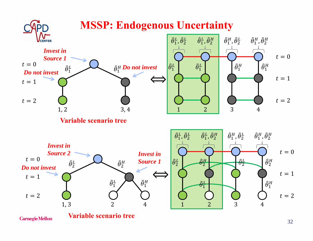
MSSP: Endogenous Uncertainty
1 2 3 4
1
2
0
, , , ,
Do not invest
1,2 3,4
Invest in Source 1
1
2
0Do not invest
Variable scenario tree
1 2 3 4
1
2
0
1,3 2 4
Invest in Source 2 Invest in
Source 1
1
2
0
, , , ,
Do not invest
Variable scenario tree

33
MSSP: Endogenous Uncertainty
33
Decision
Recourse action
Resolution of uncertainty
0 1 2
Recourse action
DecisionResolution of uncertainty
1 2 3 4
, , , ,
1
2
0,
⋁ ,
, ,
If ,
If , If ,
Superstructure scenario tree

34
MSSP: Endogenous and Exogenous Uncertainty
1 2 3 4
, , , ,
1
2
0
1 2 3 4
1
2
0
≔ ∈ ∈ Θ ,
, , … , , , … , ,, , … , ,
,
Θ ,∈∈
1, 2, … ,
≔ ∈ ∈ Ξ ,
, , … , , , … , ,, , … , ,
,
Ξ ,∈∈
1, 2, … ,
Exogenous
Endogenous
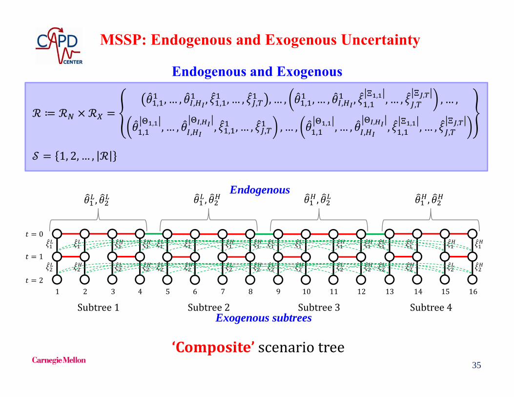
35
MSSP: Endogenous and Exogenous Uncertainty
‘Composite’ scenariotree
Endogenous and Exogenous
,
1
2
0
1 2 3 4
Subtree1
,
5 6 7 8
Subtree2
,
9 10 11 12
Subtree3
,
13 14 15 16
Subtree4
≔, , … , , , , , … , , , … , , , … , , , ,
, , … , ,, , … ,
,, , … , ,
, , , , … , , , … , ,, , … , ,
, , ,, , … , ,
,
1, 2, … ,
Endogenous
Exogenous subtrees

36
MSSP Formulation: Endogenous & Exogenous
Objectivefunction(minimizeexpectedcost)
Decision‐governing&period‐linkingconstraints
Bounds&integralityrestrictions
First‐periodNACs
s. t. , , , , , ,∈
∀ ∈ , ∈
FixedendogenousNACs
, , ∀ , ∈ , ∈ ∀ , ∈
∀ , , ∈ , ∈
, , ∀ , , ∈ , ∈ , ∈
∀ , , ∈ , ∈
min, ,
∈ , ,
∈∈
∀ ∈ , ∈ , ∈, ∈ 0,1 , ∈ , ∈ , ∈, ∈ , , , ∈ 0,1 ∀ , , ∈ , ∈
, ⇔ , , , , … , , ∀ , , ∈ , ∈ , ,
ConditionalendogenousNACs
Endogenousindistinguishabilityconstraints
1 , 1 , ∀ , , ∈ , ∈
1 ,, , 1 , ∀ , , ∈ , ∈ , , ∈
1 , 1 , ∀ , , ∈ , ∈ ,
ExogenousNACs∀ , , ∈
∀ , , ∈, , ∀ , , ∈ , ∈
VerylargenumberofconstraintsNACs
Apap, Grossmann (2015)

37
Eliminating Redundant NACs
1 2
1 5 13 1 2 5 6
1 2 3 4
Evenaftereliminatingredundantconstraints,modelsaretypicallystilltoolarge tobesolveddirectly
Specialsolutionmethods: Sequentialscenariodecomposition (SSD)heuristic Lagrangeandecomposition (LD)
Property1Symmetry
Properties2a&2bAdjacency
TransitivityProperties3&4
GroupingProperty5
Goel Gupta, Apap

38
Planningover5years Determineoptimalinvestmentandoperatingdecisions Here‐and‐nowdecisions:FPSOinstallationsandexpansions,field‐
FPSOconnections(9possible),well‐drillingschedule(30potentialwells) Recoursedecisions:Oilproductionrate
Objective: MaximizetotalexpectedNPV
GuptaandGrossmann,2014a
Totaloil/gasproduction
Oil/gasprice=?Exogenous
(Size=?)Endogenous
(Size=560MMbbls)(Size=500MMbbls)
*
FieldIFieldII
FieldIII
*www.rigzone.com
FPSO: floating production, storage and offloading
Example: Oilfield Development Planning
Piece-wise linearapproximationreservoir production

39
(2realizationsforsize)(1uncertainsize) 2endogenouscombinations
(2endogenouscombinations) (32exogenouscombinations) 64scenarios
(2realizationsforprice)(5timeperiods) 32exogenouscombinations
Totaloil/gasproduction
Oil/gasprice=?Exogenous
(Size=?)Endogenous
(Size=560MMbbls)(Size=500MMbbls)
*
FieldIFieldII
FieldIII
Example: Oilfield Development Planning
*www.rigzone.com

40
Totaloil/gasproduction
Oil/gasprice=?Exogenous
(Size=?)Endogenous
(Size=560MMbbls)(Size=500MMbbls)
FieldIFieldII
FieldIII
Example: Oilfield Development Planning
Begininstallingallinfrastructureinfirstyear:FPSO1,FPSO2
Drillingcannotstartuntilyear4duetoleadtimeforFPSOinstallation
Drillfieldswithknownsizefirst
E[NPV] = $7.166 x 10⁹
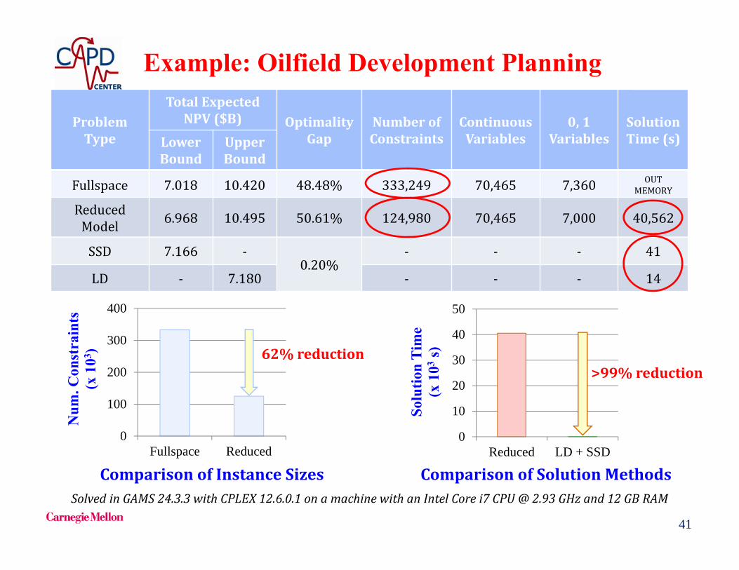
41
ProblemType
TotalExpectedNPV($B) Optimality
GapNumberofConstraints
ContinuousVariables
0,1Variables
SolutionTime(s)Lower
BoundUpperBound
Fullspace 7.018 10.420 48.48% 333,249 70,465 7,360 OUTMEMORY
SolvedinGAMS24.3.3withCPLEX12.6.0.1onamachinewithanIntelCorei7CPU@2.93GHzand12GBRAM
ComparisonofInstanceSizes
0
100
200
300
400
Fullspace Reduced
Num
. Con
stra
ints
(x
103 )
0
10
20
30
40
50
Reduced LD + SSD
Solu
tion
Tim
e (x
103
s)
>99%reduction62%reduction
ComparisonofSolutionMethods
Example: Oilfield Development Planning
ReducedModel 6.968 10.495 50.61% 124,980 70,465 7,000 40,562
SSD 7.166 ‐0.20%
‐ ‐ ‐ 41
LD ‐ 7.180 ‐ ‐ ‐ 14

42
Quality of input data?Data-Driven Modeling of Uncertainty
• Application: Two-Stage Stochastic Programming (TSSP) problem:
• Some shortcomings of the above formulation in practice: The true distribution of may not be known Need to discretize (unknown) distribution
Birge & Louveaux (2011)
How to generate scenarios given historical and forecast data?– Compute outcomes and their probabilities
Calfa, Agarwal, Grossmann, Wassick (2015)
43
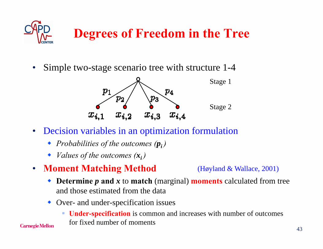
Degrees of Freedom in the Tree
• Simple two-stage scenario tree with structure 1-4
• Decision variables in an optimization formulation Probabilities of the outcomes (pi ) Values of the outcomes (xi )
• Moment Matching Method Determine p and x to match (marginal) moments calculated from tree
and those estimated from the data Over- and under-specification issues
Under-specification is common and increases with number of outcomes for fixed number of moments
Stage 1
Stage 2
(Høyland & Wallace, 2001)

44
Mitigating Under-Specification
• Each outcome has two sets of variables: and• Each moment specification has one piece of information• Consequences:
Multiple combinations of x and p satisfy moments Probabilities may not capture the shape of the underlying distribution
• Additional information: marginal (Empirical) Cumulative Distribution
Cumulative Probability

Nonlinear, nonconvex optimization problem. L1 formulation can be reformulated as an LP for fixed node values (Ji et al., 2005) 45
Min weighted error between tree and data
Probabilitiesadd up to 1
Moments calculatedfrom the tree
Covariances calculatedfrom the tree
Bounds on variables
L2 Moment Matching Problem (L2 MMP)

Nonlinear, nonconvex optimization problem. L1 formulation can be reformulated as an LP for fixed node values (Ji et al., 2005) 46
Min weighted error between tree and data
Probabilitiesadd up to 1
Moments calculatedfrom the tree
Covariances calculatedfrom the tree
Bounds on variables
ECDF information
L2 Distribution Matching Problem (L2 DMP)

47
Scenario Tree Generation and ForecastingMultistage Problems
• Final result
NLP Approach: calculate both probabilities and outcome values. LP Approach: fix outcome values, calculate probabilities.
Past Present Future

48
Motivating Example: Process Network
• Network of chemical plants
• 1 raw material (A), 1 intermediate product (B), two finished products (C and D)
• Only D can be stored and C can be purchased from elsewhere
Case 1: uncertain yield
Case 2: uncertain demands

49
Case 1: Uncertain Yield Process 1
• Historical data for production yield of facility P1
• Skewed to the right• Tail effects (extreme values) are not negligible• Approaches: Original MMP and L2 DMP (2 moments + ECDF)• TSSP, where first stage is t = 1 and second stage is t = 2, …, 4

50
Two-Stage Scenario Trees• Heuristic Approach
0.3 0.4 0.5 0.6 0.7
0.1
0.2 0.4 0.2
0.1
• L2 DMP Approach
0.14 0.66 0.76 0.83 0.90
0.02
0.21 0.28 0.270.23
Approach Expected Profit [$]Heuristic 62.77L2 DMP 72.45
51
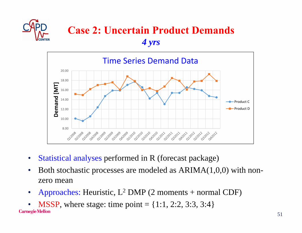
Case 2: Uncertain Product Demands4 yrs
• Statistical analyses performed in R (forecast package)• Both stochastic processes are modeled as ARIMA(1,0,0) with non-
zero mean• Approaches: Heuristic, L2 DMP (2 moments + normal CDF)• MSSP, where stage: time point = {1:1, 2:2, 3:3, 3:4}
8.00
10.00
12.00
14.00
16.00
18.00
20.00
Dem
and [M
T]Time Series Demand Data
Product C
Product D

52
• Heuristic Approach
Multi-Stage Scenario Trees
• L2 DMP Approach
NLPs: 12.3 sec (IPOPT)Heuristic L2 DMP
79.95 82.39
Expected profits [$]

53
Conclusions1. Can avoid overly conservative results in robust optimization with
linear decision rules (recourse) Cryogenic energy storage
2. To effectively solve two- or multi-stage stochastic optimization problemswith decomposition: tighten relaxation, reduce scenarios, multicut Benders
Supply chain under disruptions
3. Handling both exogenous and endogenous uncertainties in multi-stagestochastic programming yields challenging models: reduction non-anticipativityconstraints, specialized algorithms and Lagrangean decomposition
Oilfield planning
4. Historical data should be used for the generation of scenarios using moment and cumulative matching process network
Open questions/challenges:- How to extend to MINLP models with uncertainty?
- How to help users interpret solutions from these models?
54
Acknowledgments
NSF Grant CBET-1159443
Fulbright Program


