Examensarbete 30 hpJanuary 2017
Reactive Power Control for Voltage Management
MD. Shakib Hasan
Masterprogrammet i energiteknikMaster Programme in Energy Technology


Teknisk- naturvetenskaplig fakultet UTH-enheten Besöksadress: Ångströmlaboratoriet Lägerhyddsvägen 1 Hus 4, Plan 0 Postadress: Box 536 751 21 Uppsala Telefon: 018 – 471 30 03 Telefax: 018 – 471 30 00 Hemsida: http://www.teknat.uu.se/student
Abstract
Reactive Power Control for Voltage Management
MD. Shakib Hasan
This thesis presents methods for voltage management in distribution systems withhigh photovoltaic (PV) power production. The high PV penetration leads to both newchallenges such as voltage profile violation and reverse power flow, and also newopportunities. Traditionally, the voltage control in the distribution network isachieved by common devices in the networks such as capacitor banks, staticsynchronous compensators (STATCOMs) and on-load tap changers (OLTCs). Thisthesis has considered existing reactive power capable solar PV inverters together withSTATCOMs to provide voltage support for the distribution network. In this thesis,two effective coordination methods using the STATCOM and PV inverters aredeveloped in order to study their interaction and how they together can stabilize thevoltage level. Data from existing low-voltage (LV) and medium-voltage (MV) networksare used for a case study. The first control method is developed for LV network’svoltage control by means of PV inverter and STATCOM. The second control methodis developed for both LV and MV networks’ voltage control, where reactive powercontrol in PV inverters and STATCOMs are used in the LV network and onlySTATCOMs in the MV network. The control methods follow a hierarchical structurewhere reactive power compensation using PV inverters are prioritized. TheSTATCOMs, first in the LV and thereafter in the MV network in the second controlmethod, are used only when the PV inverters are not able to provide or consumeenough reactive power. This is beneficial due to the significant reduction in numbersof STATCOMs and their operation. The simulation results indicate that the proposedmethod is able to control both the over- and undervoltage situations for the testdistribution networks. It is also shown that reactive power supply at night by the PVinverters can be an important resource for effective voltage regulation by using theproposed coordinated voltage control method.
Tryckt av: Ångströmlaboratoriet, Uppsala UniversitetMSc ET 17002Examinator: Joakim WidénÄmnesgranskare: Juan de SantiagoHandledare: Rasmus Luthander


Division of Solid State PhysicsBuilt Environment Energy Systems Group
Ångströmlaboratoriet, Lägerhyddsvägen 1Uppsala University
Box: 534, 75121, Uppsala
Tel.: +46 (0)18 471 3024 Fax: +46 (0)18 471 3270
Name of Student : MD. Shakib Hasan
Sernanders väg. 05/532
75261, Uppsala
Degree Name : Master of Science in Energy Technology
Title of Thesis : Reactive Power Control for Voltage Management
Supervisor : Rasmus Luthander, PhD student
Scientific Reader : Juan de Santiago, PhD
Examiner : Joakim Widén, Associate Professor
Beginning : 17.01.2017
End : 21.06.2017
Date of Presentation : 07.06.2017
Joakim Widén

Contents
1 Introduction 1
1.1 Background . . . . . . . . . . . . . . . . . . . . . . . . . . . . . . . . 1
1.2 Challenges and motivations . . . . . . . . . . . . . . . . . . . . . . . 2
1.3 Literature review on voltage control in distribution network . . . . . . 3
1.3.1 Devices currently operating as compensators . . . . . . . . . . 4
1.3.2 Current Volt/VAR management regulation systems . . . . . . 5
1.4 Thesis objectives . . . . . . . . . . . . . . . . . . . . . . . . . . . . . 7
1.5 Research approach . . . . . . . . . . . . . . . . . . . . . . . . . . . . 7
1.6 Limitations . . . . . . . . . . . . . . . . . . . . . . . . . . . . . . . . 8
1.7 Boundary conditions . . . . . . . . . . . . . . . . . . . . . . . . . . . 8
1.8 Thesis outline . . . . . . . . . . . . . . . . . . . . . . . . . . . . . . . 9
2 Reactive Power Compensation Devices and Test Grid 11
2.1 Photovoltaic (PV) inverter . . . . . . . . . . . . . . . . . . . . . . . . 11
2.1.1 Inverter reactive power range . . . . . . . . . . . . . . . . . . 12
2.1.2 Reactive power control methods of PV inverter . . . . . . . . 13
2.2 Static synchronous compensator (STATCOM) . . . . . . . . . . . . . 13
2.2.1 Power semiconductor devices . . . . . . . . . . . . . . . . . . . 14
2.2.2 Operation principle . . . . . . . . . . . . . . . . . . . . . . . . 14
2.2.3 Control modes . . . . . . . . . . . . . . . . . . . . . . . . . . . 16
2.3 Grid codes . . . . . . . . . . . . . . . . . . . . . . . . . . . . . . . . . 17
2.4 Test grid . . . . . . . . . . . . . . . . . . . . . . . . . . . . . . . . . . 18vii

Page viii CONTENTS
3 Modelling of Reactive Power Control Methods and Proposed Co-
ordinated Voltage Control Algorithm 19
3.1 PV inverter control method - Q(U) . . . . . . . . . . . . . . . . . . . 19
3.2 STATCOM control method . . . . . . . . . . . . . . . . . . . . . . . 22
3.3 Proposed coordinated voltage control algorithm . . . . . . . . . . . . 24
3.3.1 Scenario I : Voltage control algorithm for the Low Voltage
(LV) grid . . . . . . . . . . . . . . . . . . . . . . . . . . . . . 24
3.3.2 Scenario II : Voltage control algorithm for the LV grid and
Medium Voltage (MV) grid . . . . . . . . . . . . . . . . . . . 24
4 Simulation and Results 27
4.1 Grid simulation for scenario I and II . . . . . . . . . . . . . . . . . . 27
4.1.1 Results for scenario I . . . . . . . . . . . . . . . . . . . . . . . 28
4.1.2 Results for scenario II . . . . . . . . . . . . . . . . . . . . . . 39
4.2 PV inverter - reactive power (Q) support at night . . . . . . . . . . . 45
5 Discussion 47
5.1 Methodology and input data . . . . . . . . . . . . . . . . . . . . . . . 47
5.2 System effects and compensation techniques . . . . . . . . . . . . . . 49
6 Conclusion and Future Work 51
6.1 Conclusion . . . . . . . . . . . . . . . . . . . . . . . . . . . . . . . . . 51
6.2 Future work . . . . . . . . . . . . . . . . . . . . . . . . . . . . . . . . 52
7 Acknowledgements 53
Bibliography 54
Appendix 58
A System data 59
A.1 Grid code data . . . . . . . . . . . . . . . . . . . . . . . . . . . . . . 59
A.2 Summary on parameter settings for compensators . . . . . . . . . . . 59
A.3 PV system data . . . . . . . . . . . . . . . . . . . . . . . . . . . . . . 60
List of Figures
2.1 Photovoltaic (PV) power plant equivalent circuit. . . . . . . . . . . . 12
2.2 STATCOM schematic representation. . . . . . . . . . . . . . . . . . . 14
2.3 (a): STATCOM equivalent circuit. (b): A typical U-I characteristics
of STATCOM. . . . . . . . . . . . . . . . . . . . . . . . . . . . . . . . 15
2.4 Generic single-line diagram of test grid. . . . . . . . . . . . . . . . . . 18
3.1 Standard reactive power methods- Q(U). . . . . . . . . . . . . . . . . 20
3.2 Flow chart with the implementation of the Q(U) method. . . . . . . . 21
3.3 STATCOM equivalent circuit. . . . . . . . . . . . . . . . . . . . . . . 22
3.4 Flow chart with the implementation of the STATCOM control method. 23
3.5 Control flow chart for the Low Voltage (LV) grid. . . . . . . . . . . . 25
3.6 Control flow chart for the Low Voltage (LV) and Medium Voltage
(MV) grid. . . . . . . . . . . . . . . . . . . . . . . . . . . . . . . . . . 26
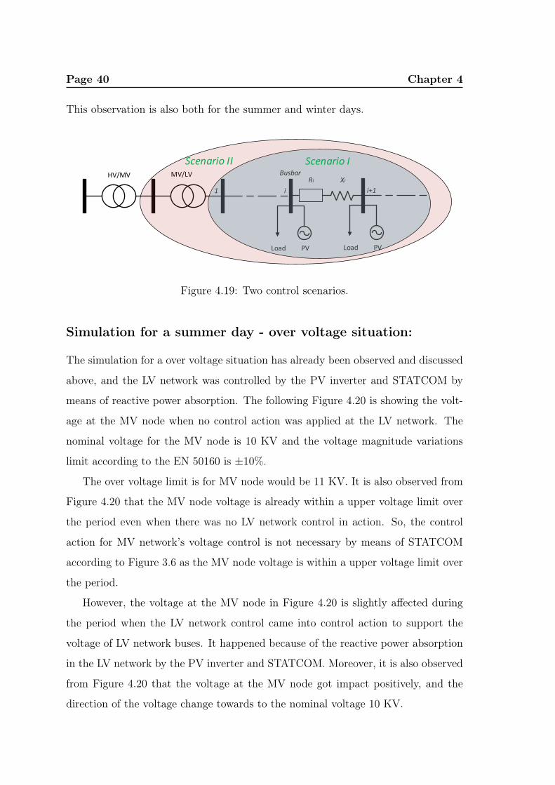
4.1 Two control scenarios. . . . . . . . . . . . . . . . . . . . . . . . . . . 28
4.2 Voltage in the LV grid buses before applying the voltage control.
Total number of buses 93 and each line represents the hourly buses
voltage. . . . . . . . . . . . . . . . . . . . . . . . . . . . . . . . . . . 29
4.3 Voltage in the critical grid bus 48 after applying the voltage control
by the PV inverter. . . . . . . . . . . . . . . . . . . . . . . . . . . . . 29
4.4 Reactive power absorption at bus 48 by the PV inverter. . . . . . . . 30
4.5 Voltage in the grid buses after applying the voltage control by PV
inverter. Each line represents the hourly buses voltage. . . . . . . . . 30ix

Page x LIST OF FIGURES
4.6 Voltage in the grid bus 48 after applying the voltage control by the
PV inverter and Static Synchronous Compensator (STATCOM). . . . 31
4.7 Reactive power absorption by the STATCOM. . . . . . . . . . . . . . 32
4.8 Voltage in the grid buses after applying the voltage control by the PV
inverter and STATCOM. Each line represents the hourly buses voltage. 32
4.9 Total reactive power absorption by the PV inverter and STATCOM. . 33
4.10 Voltage at all the grid buses before applying the control. Each line
represents the hourly buses voltage. . . . . . . . . . . . . . . . . . . . 34
4.11 Voltage at all the weak grid buses before applying the voltage control.
Each line represents the each bus voltage. . . . . . . . . . . . . . . . 35
4.12 Voltage at all the weak grid buses after applying the voltage control
by the PV inverter. Each line represents the each bus voltage. . . . . 35
4.13 Reactive power injection by the PV inverter. . . . . . . . . . . . . . . 36
4.14 Voltage at all the grid buses after applying the voltage control by PV
inverters. Each line represents the hourly buses voltage. . . . . . . . . 36
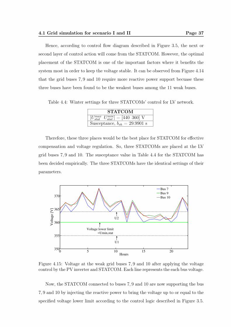
4.15 Voltage at the weak grid buses 7, 9 and 10 after applying the voltage
control by the PV inverter and STATCOM. Each line represents the
each bus voltage. . . . . . . . . . . . . . . . . . . . . . . . . . . . . . 37
4.16 Reactive power generation by the STATCOM. . . . . . . . . . . . . . 38
4.17 Voltage at all the grid buses after applying the voltage control by the
PV inverter and STATCOM. Each line represents the hourly buses
voltage. . . . . . . . . . . . . . . . . . . . . . . . . . . . . . . . . . . 38
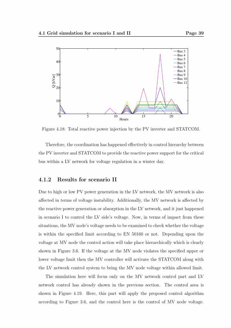
4.18 Total reactive power injection by the PV inverter and STATCOM. . . 39
4.19 Two control scenarios. . . . . . . . . . . . . . . . . . . . . . . . . . . 40
4.20 Voltage at the Medium Voltage (MV) node before and after the Low
Voltage (LV) network control action. . . . . . . . . . . . . . . . . . . 41
4.21 Voltage at the MV node after the LV network control action. . . . . . 42
4.22 Voltage at one MV node before and after applying the MV network
control. . . . . . . . . . . . . . . . . . . . . . . . . . . . . . . . . . . 43
4.23 Q absorption by the STATCOM at one MV node. . . . . . . . . . . . 43
LIST OF FIGURES Page xi
4.24 Voltage at all MV nodes before and after applying the MV network
control. . . . . . . . . . . . . . . . . . . . . . . . . . . . . . . . . . . 44
4.25 Q absorption at all MV nodes by the STATCOM. . . . . . . . . . . . 44
4.26 P and Q scenarios for the LV grid bus 3. . . . . . . . . . . . . . . . . 46
4.27 Voltage at the LV grid bus 3 before and after Q compensation by the
PV inverter. . . . . . . . . . . . . . . . . . . . . . . . . . . . . . . . . 46
A.1 PV systems’ P and Q capacity information. . . . . . . . . . . . . . . 60


List of Tables
2.1 Summary of the test grid characteristics. . . . . . . . . . . . . . . . . 18
4.1 Summer settings for PV inverter control for LV network. . . . . . . . 28
4.2 Summer settings for STATCOM control for LV network. . . . . . . . 31
4.3 Winter settings for PV inverter control for LV network. . . . . . . . . 34
4.4 Winter settings for three STATCOMs’ control for LV network. . . . . 37
4.5 Parameter settings used for STATCOM control during summer for
MV network. . . . . . . . . . . . . . . . . . . . . . . . . . . . . . . . 43
A.1 Allowed voltage limit in steady-state for both MV and LV network. . 59
A.2 Parameter settings used seasonally for PV inverters and STATCOMs
for LV and MV network control. . . . . . . . . . . . . . . . . . . . . . 59
xiii

Glossary
AC Alternating Current
DC Direct Current
DER Distributed Energy Resource
DG Distributed Generation
FACTS Flexible Alternating Current Transmission
Systems
GGC German Grid Codes
GTO Gate Turn Off
IGBT Insulated Gate Bipolar Transistors
IGCT Integrated Gate Communicated Thyristors
LV Low Voltage
MV Medium Voltage
OLTC On Load Tap Changers
PCC Point of Common Coupling
PV Photovoltaic
SC Shunt Capacitor
STATCOM Static Synchronous Compensator
SVC Static Var Compensator
VSC Voltage Source Converter


List of Symbols
θi phase angle of the grid bus voltage [radian]
θsh phase angle of the STATCOM voltage [radian]
θgi phase angle of the inverter voltage output [radian]
cosφref reference power factor
cosϕ(P ) power factor control dependent on the active power injection
bsh susceptance of the STATCOM [siemens (s)]
gsh conductance of the STATCOM [siemens, (s)]
Pi active power in the grid busbar [W]
Psh active power of STATCOM [W]
Pn nominal PV power production capacity [W]
P refi reference active power from inverter [W]
Q(U) local reactive power control dependent on voltage
Qi reactive power in the grid busbar [VAR]
QIi reactive power of inverter [VAR]
Qref , Qref reference signal for reactive power [VAR]
QPCC measured reactive power at PCC [VAR]
−Qmax maximum reactive power absorption [VAR]xvii
Page xviii Glossary
+Qmax maximum reactive power generation [VAR]
QSpecsh reference signal for reactive power [VAR]
Qsh reactive power from STATCOM [VAR]
Q(U) reactive power control dependent on voltage [VAR]
Qrefstat reference signal for reactive power from STATCOM [VAR]
QrefPV reference signal for reactive power from PV inverter [VAR]
Si apparent power of inverter [VA]
Ush voltage of the STATCOM [V]
Ugi inverter output voltage [V]
Us, Ui voltage of grid bus [V]
USpeci , Uref reference signal for bus voltage [V]
U1, U2, U3, U4 reference voltages for Q(U) control method [V]
Umeas measured bus voltage [V]
Umaxsh maximum reference voltage for STATCOM [V]
Uminsh minimum reference voltage for STATCOM [V]
Xi transformer and line reactance [Ω]
Xsh reactance of STATCOM [Ω]
Zsh impedance of the STATCOM [Ω]
Chapter 1
Introduction
1.1 Background
Voltage stability is one of the major concerns when planning and operating a modern
power system, and it has earned much attention in recent years due to the increasing
number of renewable Distributed Generation (DG) units. One of the fastest growing
and cheap energy resources among the available renewable energy sources is solar
Photovoltaic (PV) systems. Solar PV energy is considered as an important energy
resource to meet the increasing medium and long term global energy demand [1].
PV systems can be integrated into high, medium and low voltage grids although
they are mainly connected to the MV and LV grids. In the recent years, high
penetration of PV systems is happening mostly in the LV grid networks because of
their highly decentralized nature. This has led to challenges for the grid operators
to maintain a stable power grid and comply with different grid codes. For example,
according to [2] which is European grid standard EN 50160, and the voltage range
has to be within ±10% of rated voltage under normal operating conditions. One of
the main challenges is voltage instability caused by the large number of distributed
PV systems with their intermittent nature of power production [1].
In order to achieve the voltage stability, the power system needs to be operated
within an acceptable voltage range even under disturbances. The very known dis-
turbances in power system are sudden changes in loads, switches in loads, changes
or losses in supply. Besides that, disturbances also occur when reactive power flows1
Page 2 Chapter 1
through the transmission lines and modify the line and bus voltages [2].
The main focus of this thesis is to propose an effective coordinated voltage control
method by using two different reactive power compensation techniques to deal with
the unwanted voltage problem associated with high PV penetrations. It is worth
mentioning that the proposed control method will not only provide the voltage con-
trol scheme for LV network, moreover, it has considered the MV distribution grids’
voltage control scheme as well. This thesis work will concentrate on the Swedish
municipality of Herrljunga. It is important to keep the voltage under acceptable
limits according to European standard EN 50160 regulation ±10% for both the LV
and MV network while trying to integrate large number of PV systems into the
existing power grid. The information about the studied grid structure and other
grid related parameters are not revealed here in this report for the purpose of grid
security.
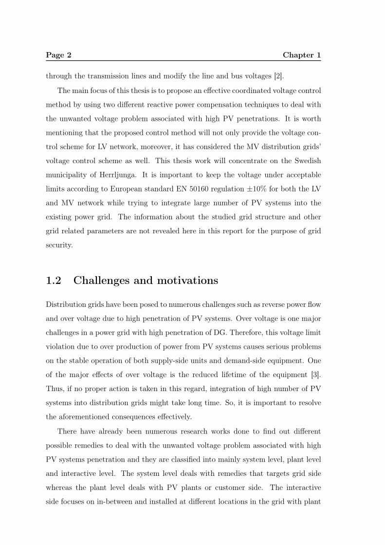
1.2 Challenges and motivations
Distribution grids have been posed to numerous challenges such as reverse power flow
and over voltage due to high penetration of PV systems. Over voltage is one major
challenges in a power grid with high penetration of DG. Therefore, this voltage limit
violation due to over production of power from PV systems causes serious problems
on the stable operation of both supply-side units and demand-side equipment. One
of the major effects of over voltage is the reduced lifetime of the equipment [3].
Thus, if no proper action is taken in this regard, integration of high number of PV
systems into distribution grids might take long time. So, it is important to resolve
the aforementioned consequences effectively.
There have already been numerous research works done to find out different
possible remedies to deal with the unwanted voltage problem associated with high
PV systems penetration and they are classified into mainly system level, plant level
and interactive level. The system level deals with remedies that targets grid side
whereas the plant level deals with PV plants or customer side. The interactive
side focuses on in-between and installed at different locations in the grid with plant
1.3 Literature review on voltage control in distribution network Page 3
components and it requires the communication structures to link to the decision
making units. The system level solution includes mainly grid reinforcement and On
Load Tap Changers (OLTC), whereas the plant level remedies includes plant level
storage, active power curtailment, reactive power control and Flexible Alternating
Current Transmission Systems (FACTS) devices such as Static Var Compensator
(SVC) [3]. The voltage regulation through reactive power control by the PV inverter
is economical and preferred over other remedies because there is no technological
barrier to do this. It is easier to modulate the PV inverter to have reactive power
similar to producing active power and requires no additional physical equipment.
For example, Germany have allowed reactive power contribution from PV in-
verter in the LV grid. The voltage regulation methods encouraged by German Grid
Codes (GGC) such as cosϕ(P ) and Q(U) have already been studied and imple-
mented on the LV grid in Germany [3]. Therefore, one of the main focuses of this
thesis is to use reactive power contribution from PV inverter for LV grids’ voltage
regulation along with the Static Synchronous Compensator (STATCOM).
Furthermore, due to the high number of PV systems in the power systems, the
power flow is not unidirectional anymore. This changes the active and reactive
power responses of LV grids to voltage variations in the MV grids. The changes in
the voltage-power characteristic at the LV grids may affect the behavior of the MV
grids. So, this thesis will also address how this high penetration of PV systems in
LV grids would have impact onto MV grids and how to resolve this phenomenon
with the help of coordinated control mechanism. Consequently, it is necessary to
find a coordinated reactive power control method that can effectively control the
voltage profile of the MV grids and LV grids with the high density of PV systems.
1.3 Literature review on voltage control in distribu-
tion network
In the recent years, several studies have been carried out on how to mitigate the
voltage rise caused by PV generation, since voltage rise is one of the most impor-

Page 4 Chapter 1
tant limitations towards effective integration [1],[4]. Two aspects are importantly
considered in order to achieve the overall grid stability: types of devices operating
as compensators and its overall control management [2].
1.3.1 Devices currently operating as compensators
Voltage regulation is performed in two different ways- shunt and series regulation.
The shunt regulation includes all types of reactive compensation devices connected
in shunt with the grid. On the other hand, the series regulation includes voltage
regulators and reactive compensators connected in series with the grid [2].
• Voltage regulators
Traditionally, the voltage regulators are the most common devices used in
grids, and it is the earliest device implemented for voltage drop compensation.
It is mechanically driven and regulates the voltage by changing the number of
windings. However, a voltage regulator according to [5] consists of a tapped
auto-transformer and a tap changer. OLTCs are the most common type and
used for a very long period of time. OLTCs are connected to the feeder in series,
and any change in the secondary side would increase the voltage downstream
along the feeder [2].
• Capacitor bank
Capacitor banks are the cheapest and simplest from a technical perspective to
be used as compensators. These devices are able to compensate loads with a
poor power factor [2].
• STATCOM
The STATCOM is a fast-acting and precise device. It supplies or absorbs
adjustable amounts of reactive power to the networks for the voltage regulation
whenever it requires. The amount and the direction of the reactive power flow
are regulated by these devices. They adjust the magnitude and the phase
of the reactive component of the current flowing through their Alternating
Current (AC) side [2].

1.3 Literature review on voltage control in distribution network Page 5
• PV inverter
Reactive power compensation by the PV inverter is another way of voltage
regulation. The operational principles of PV inverter are still lack of consensus
[6]. Hoever, the reactive power control by the grid-connected inverters on
LV distribution networks has already been considered by some countries for
voltage such as Germany [4].
• SVC
Over voltage due to high PV power generation in LV network can be suppressed
by using the SVC and it is one of the members of FACTS family. However,
installing the SVCs in the network is quite an expensive [3].
• Other components
Some other devices are currently used in voltage control of grids such as active
filters, power factor controllers, new energy storage loads, or electric vehicles
[2].
These control devices have been used so far to tackle the voltage rise issue for
connecting solar PV systems into network either by using one compensation device
locally or co-ordination among several compensation devices at different level of
grid network. Most of the literature or scientific works in [2],[7],[8],[9] so far found
have focused on coordinated control based on theoretical simulations by using PV
inverters with the SVC, OLTC or Shunt Capacitor (SC). However, very few studies
on coordinated voltage control in a distribution grid using PV inverters and STAT-
COMs have been made. This thesis will therefore focus on coordinated voltage
control by using the PV inverters and STATCOM at the LV and MV levels in order
to keep the network voltage profile according to grid standard.
1.3.2 Current Volt/VAR management regulation systems
Volt/VAR management regulation is a technique that has been used for a long
time in power distribution systems and deals with the voltage and reactive power
control [2]. The devices that have been mentioned earlier are used to regulate the

Page 6 Chapter 1
instantaneous voltage by controlling the reactive power flow. According to European
standard EN 50160 regulation, the voltage should be within ±10% of rated voltage
under normal operating conditions. Currently, Volt/VAR management is being used
to keep the system within these levels by the distribution operator [2].
There are common types of control methods or structures that have been found
in the literature which are used to control the compensator devices according to [10].
• Decentralized control
The control actions are derived locally at each node to which Distributed
Energy Resource (DER) is connected to provide voltage support from DERs.
In this case only the local information is used without the knowledge of how
control action effect the overall system because of no exchange of information
[10].
• Centralized control
The control decision in centralized control system is made only by the co-
ordinator/central controller and the overall control strategy is stored at the
central controller. Usually, it collects the complete information from the whole
network and takes control action based on the data collected [10].
• Hierarchical control
A hierarchical control is formed according to the existing structure of the
grid network. The coordinator situated at the higher level calculates the set
points, which are the reference signals for the lower level local controller. Thus
it consists of multiple control layers, so in the case where it is not enough
with the first control layer, the system continues with the next control layer.
The main role of the higher level controllers is to ensure the consistent control
behavior between the lower local controllers which will lead to improved overall
global performance [10].
This hierarchical control structure will be used in this thesis and the proposed
solution will consider the different combinations of PV inverters and STAT-
COM, and it will define in what order they should contribute to the voltage

1.4 Thesis objectives Page 7
regulation for MV and LV grid network. The total control structure will be
discussed in details in the subsequent chapter.
The achievement of this coordination will be carried out through simulations
on a realistic MV and LV Swedish distribution network. In simulation, two
scenarios will be tested: coordinated control for LV networks by PV inverter
and STATCOM; and coordinated control for both MV and LV networks by
PV inverter and STATCOM.
1.4 Thesis objectives
This thesis attempts to answer the following research objectives:
• Examine how power production in the LV grids from high number of PV sys-
tems would have the impact on LV and MV grids in terms of voltage instability.
• Examine actions that can be taken to suppress the voltage instability.
• Design a coordinated reactive power control model for PV interver and STAT-
COM to avoid over- and undervoltage situation in distribution grids.
• Evaluate the proposed model using the real data from Swedish MV and LV
distribution grids.
1.5 Research approach
The penetration of large scale PV systems into existing power distributon grid is a
growing trend, and therefore this thesis work examines voltage rise and drop in both
MV and LV grids. The PV inverters and STATCOM will be investigated as means
of dealing with these voltage variation problems at different level of the distribu-
tion network. Afterwards, a coordinated voltage control method will be proposed
and demonstrated. The development and implementation of the proposed control
method are based on modelling and simulations. The Matlab/Simulink software will
be used for simulation and the developed control method will be examined with a
Page 8 Chapter 1
case study. The solar PV is connected to the LV side of the studied grid in which
PV power plants will represent the generation part, and loads also connected in the
LV side represent the consumption part. A reactive power regulation of solar PV
model would be developed for the local voltage support at plant level. In addition,
the STATCOM will also provide the voltage control capabilities for both the MV
and LV grids.
Finally, the coordinated voltage control algorithm will be tested on the test grid
with a view to assess the consequences of control on node voltages and should allow
the system to operate under the conditions defined by grid codes.
1.6 Limitations
This thesis work is limited by several different factors:
• This work only addresses technical aspects of possible solutions for keeping
the voltage profile within the allowed voltage limit. The financial aspects are
not analyzed here.
• The reactive power control model for STATCOM is considered as an ideal,
and thus losses are not taken into consideration.
1.7 Boundary conditions
This thesis work has some boundary conditions that has been considered during the
control algorithm development and simulation:
• The developed coordinated voltage control algorithm is tested and simulated
for one LV network and 252 nodes of MV networks.
• The simulation has been carried out for one winter day and one summer day.
• The control of the PV inverters and the STATCOM overlapped. The methods
works if the inverters get a signal from the STATCOM saying that they are
"on" and that they should continue providing maximum reactive power until
they disconnect.
1.8 Thesis outline Page 9
• The capacity limit for the STATCOM is not considered for reactive power
generation/absorption.
• The line losses and line capacity analysis are not part of this study.
1.8 Thesis outline
The rest of this thesis is organized as follows:
Chapter 2 briefly describes about two reactive power compensation devices (PV
inverter and STATCOM), discusses about the grid codes, and presents brief infor-
mation about the test grid.
Chapter 3 depicts the modelling of reactive power control methods for PV inverter
and STATCOM based on voltage droop characteristics, and presents the proposed
coordinated voltage control method for the LV network and MV network.
Chapter 4 presents the simulation of the test grid and the results.
Chapter 5 provides the discussion.
Chapter 6 highlights the main conclusions of the thesis and summarizes the ideas
for future research work.

Page 10 Chapter 1

Chapter 2
Reactive Power Compensation
Devices and Test Grid
Introduction
One of the main sources of voltage collapse is the lack of reactive power and this
causes voltage instability in a power system [11]. To overcome the voltage instability
issue the reactive power flow control method is one of the economical choices which
has already been mentioned in the previous chapter. It is also mentioned previously
that the most of the studies found in the literature focus on control strategies that
integrate the coordinated control operation among the OLTCs, PV inverters, SVCs
and SCs [2],[7],[8],[9]. However, the research was limited to assess the technical
potential of coordinated control strategies that integrate both the PV inverter and
STATCOM. That is why these two reactive power sources have been chosen to
supply reactive power: PV inverter and STATCOM. This chapter will discuss about
the PV inverter, STATCOM, grid codes and the test grids.
2.1 Photovoltaic (PV) inverter
It is already known that the fast expansion of PV systems into the lower parts of
the grid has raised several concerns to the grid operator [3]. One of the concerns is
grid voltage stability. The grid operators have to impose strict operational rules on11
Page 12 Chapter 2
PV systems in order to keep the grid voltage stable. As a consequence they have
proposed to the PV system manufacturers that the PV inverters should have the
capability to control the voltage. One of the grid support functions that has been
included into the PV inverters is the reactive power capability to stabilize the grid
voltage [12].
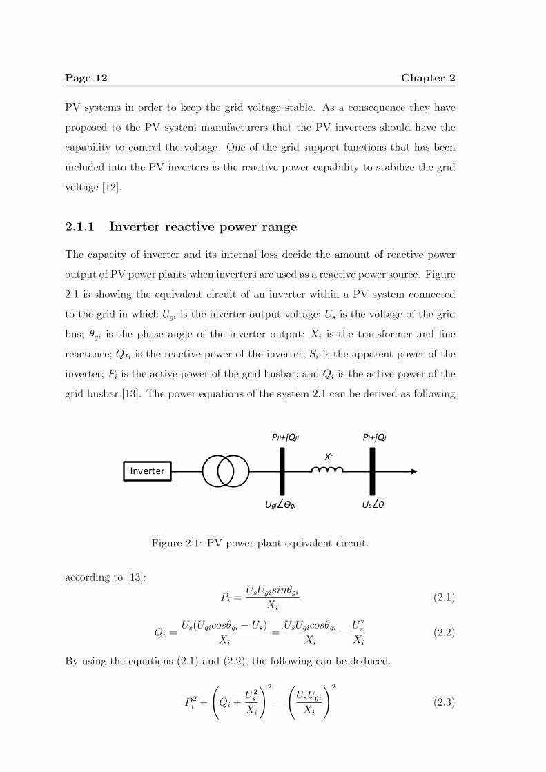
2.1.1 Inverter reactive power range
The capacity of inverter and its internal loss decide the amount of reactive power
output of PV power plants when inverters are used as a reactive power source. Figure
2.1 is showing the equivalent circuit of an inverter within a PV system connected
to the grid in which Ugi is the inverter output voltage; Us is the voltage of the grid
bus; θgi is the phase angle of the inverter output; Xi is the transformer and line
reactance; QIi is the reactive power of the inverter; Si is the apparent power of the
inverter; Pi is the active power of the grid busbar; and Qi is the active power of the
grid busbar [13]. The power equations of the system 2.1 can be derived as following
Inverter
Ugi Ѳgi Us 0
PIi+jQIi Pi+jQi
Xi
Figure 2.1: PV power plant equivalent circuit.
according to [13]:
Pi =UsUgisinθgi
Xi
(2.1)
Qi =Us(Ugicosθgi − Us)
Xi
=UsUgicosθgi
Xi
− U2s
Xi
(2.2)
By using the equations (2.1) and (2.2), the following can be deduced.
P 2i +
(Qi +
U2s
Xi
)2
=
(UsUgi
Xi
)2
(2.3)

2.2 Static synchronous compensator (STATCOM) Page 13
When the value of Qi = 0 and then the equation (2.3) becomes:
Pi =
√√√√(UsUgi
Xi
)2
−
(Us
Xi
)2
=Us
Xi
√U2gi − U2
s (2.4)
The equation (2.3) gives the range of reactive power that the inverter can supply to
the bus bar connected to the grid and which can be defined by:
−
√√√√(UsUgi
Xi
)2
− P 2i −
U2s
Xi
≤ Qi ≤
√√√√(UsUgi
Xi
)2
− P 2i −
U2s
Xi
(2.5)
Inverters normally operate at rated active power to maintain the active power output
of the PV system, and therefore the inductive and capacitive reactive power output
range is limited for an inverter [13].
2.1.2 Reactive power control methods of PV inverter
There are four different reactive power control methods that have been suggested
according to [14]: fixed power factor, constant reactive power, power factor control
dependent on the active power injection cosϕ(P ), and local reactive power control
dependent on voltage Q(U). The last technique is of the interest for this study as
the Q(U) method directly use the local voltage information to stabilize the weak
bus voltage.
This thesis focuses on the voltage control by the PV inverter using Q(U) method.
This control action maintains the acceptable voltage range at the PCC by providing
the reactive power into the network from PV inverter. The details of Q(U) control
method modelling is discussed in the next chapter.
2.2 Static synchronous compensator (STATCOM)
STATCOM is the most widely used member of FACTS, and is usually used as a
source to provide reactive power to control the transmission voltage. This reactive
power compensation is mainly shunt compensation with the AC system. The reac-

Page 14 Chapter 2
tive power compensation by the STATCOM is based on Voltage Source Converter
(VSC) which is much faster and has a bigger range of control because of the usage of
semiconductor switches instead of mechanical switches [15]. In the following section
the details about the STATCOM are presented.
2.2.1 Power semiconductor devices
A STATCOM is usually consists of one VSC with a capacitor on a Direct Current
(DC) side of the converter and one shunt connected transformer which is shown in
Figure 2.2. The VSC is built with thyristors with turn-off capability like Gate Turn
Off (GTO) or today’s advanced Integrated Gate Communicated Thyristors (IGCT)
or with Insulated Gate Bipolar Transistors (IGBT) based converter [15].
Uk
Bus k
IvR
EvR
UDC+
-
Figure 2.2: STATCOM schematic representation.
2.2.2 Operation principle
Traditionally, the STATCOM can be used as synchronous voltage source since its
output voltage can be controlled as desired as presented in Figure 2.2. Here the
assumption is that there is no exchange of active power between STATCOM and
the grid, and the operation is lossless, so the voltage of the STATCOM controller
and the grid voltage is in phase. The flow of current through the STATCOM is
dependent on the voltage difference between the grid and the STATCOM. If the
compensator voltage magnitude is smaller than the voltage at the connection point,
reactive power will be consumed by the STATCOM. On the other hand, if the
situation is opposite, reactive power will be delivered to the grid [15]. This principle
2.2 Static synchronous compensator (STATCOM) Page 15
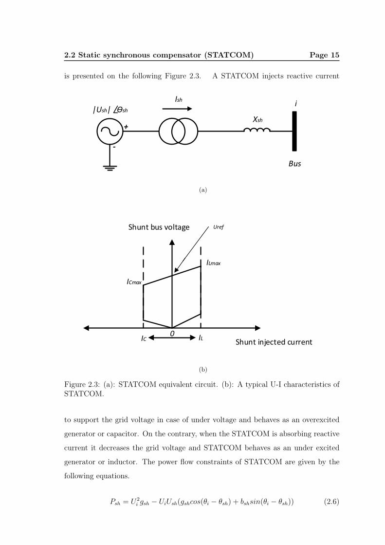
is presented on the following Figure 2.3. A STATCOM injects reactive current
Xsh
i
+
-
|Ush| Ѳsh
Bus
Ish
(a)
Shunt injected current
ILmax
ICmax
0IC IL
UrefShunt bus voltage
(b)
Figure 2.3: (a): STATCOM equivalent circuit. (b): A typical U-I characteristics ofSTATCOM.
to support the grid voltage in case of under voltage and behaves as an overexcited
generator or capacitor. On the contrary, when the STATCOM is absorbing reactive
current it decreases the grid voltage and STATCOM behaves as an under excited
generator or inductor. The power flow constraints of STATCOM are given by the
following equations.
Psh = U2i gsh − UiUsh(gshcos(θi − θsh) + bshsin(θi − θsh)) (2.6)

Page 16 Chapter 2
Qsh = −U2i bsh − UiUsh(gshsin(θi − θsh)− bshcos(θi − θsh)) (2.7)
in which Ui and θi are the voltage of the bus and the angle of the bus voltage
to which the STATCOM is connected. Ush and θsh are the voltage and the angle of
the STATCOM and gsh + jbsh = 1/Zsh.
2.2.3 Control modes
There are various control modes of STATCOM operation through which the control
of reactive power flow is provided by STATCOM. The flow of reactive power control
can be realized in one of the following control modes by the STATCOM.
• Reactive power
This control method focuses on direct reactive power injection or absorption to
the local bus, to which the STATCOM is connected according to the specified
reference by the distribution operator [15]. This control mechanism can be
expressed mathematically as follows:
Qsh −QSpecsh = 0 (2.8)
in which the QSpecsh is the reference signal for reactive power and Qsh can be
found from equation (2.7).
• Voltage droop characteristics
This control strategy is based on voltage/reactive power slope characteristics
and the setting of target voltage at Point of Common Coupling (PCC) is set by
the distribution operator according to the grid code [15]. The voltage control
is specified as follows:
Ui − USpeci = 0 (2.9)
in which the USpeci is the reference voltage signal that has to maintained at
PCC and Ui is the ith bus voltage.
• Power factor
This mode of control is the modification of power factor at the PCC in which
2.3 Grid codes Page 17
the STATCOM is connected and the control constraint can be realized by the
following equation [15].
Qref −QPCC = 0 (2.10)
The Qref is the reference signal for reactive power that can be achieved by the
following equation (2.11) and QPCC is the measured reactive power at PCC.
Qref =√S2 − P 2
PCC =
√P 2PCC
cos2φref
− P 2PCC (2.11)
in which PPCC is active power at the PCC and cosφref is the desired reference
power factor.
This thesis focuses on the voltage control by the STATCOM at the PCC in which the
PV inverter is not capable anymore to maintain the voltage within the specified limit.
Therefore, voltage droop characteristics control mode will be used to control the
STATCOM. This control mode maintains a constant voltage at the PCC considering
the error between the voltage reference and the measured voltage by providing the
reactive power into the network. The details about the STATCOM control method
modelling is discussed in the next chapter.
2.3 Grid codes
The European grid code EN 50160 is the standard that deals with the important
grid requirements to provide quality power from supplier side to the customer side.
One of the important requirements is to characterize the voltage parameters for the
public distribution networks. According to standard EN 50160, there are several
voltage parameters which needs to be fulfilled for the proper grid operation where
voltage magnitude variations, rapid voltage changes, supply voltage dips, flicker, sup-
ply interruptions are the most important ones. However, according to this standard,
the voltage magnitude variations at the customer’s PCC in public LV and MV elec-
tricity distribution network have to be maintained within ±10%. However, in the
appendix section A.1, the values for the allowed voltage limit for LV and MV grids

Page 18 Chapter 2
are provided.
2.4 Test grid
The investigation of voltage instability is performed on the grid of Swedish munic-
ipality of Herrljunga. The grid consists of two MV networks and 338 LV networks.
But the test grid considered for this study will focus on 252 nodes of one MV grid
and one LV network under one node of the MV network. The generic single-line
diagram of the test grid is shown in Figure 2.4. Finally, a coordinated voltage
control method will be proposed by using two VAR compensation devices in the
distribution network to overcome the voltage instability. One compensatator would
be the existing PV inverter in the system and the other compensatator would be
the STATCOM. Some information about the test grid parameters are summarized
in the following Table 2.1.
Xi
i
Busbar
MV/LVHV/MV
PVLoad PVLoad
1 i+1
Ri
Figure 2.4: Generic single-line diagram of test grid.
Table 2.1: Summary of the test grid characteristics.
Test Grid (HERRLJUNGA) CharacteristicsMV LV
Voltage 10 KV 0.4 KVGrid topology mesh radialNumber of buses* - 93Number of nodes** 252 -
* : grid bus of the LV network is the connection point where PV/STATCOM/load are
connected, and there are 93 buses in total for the considered LV network.
** : node of the MV network is the connection point where LV network is connected, and
there are 252 nodes in total of the considered one MV network.

Chapter 3
Modelling of Reactive Power Control
Methods and Proposed Coordinated
Voltage Control Algorithm
Introduction
This chapter describes the modelling of reactive power control methods of the con-
sidered compensation devices which are PV inverter and STATCOM. It also presents
the proposed coordinated voltage control algorithm for LV and MV network.
3.1 PV inverter control method - Q(U)
As already mentioned earlier, the reactive power capabilities of solar inverters can
be used to maintain the voltage level within the specified limits. In chapter 2,
several reactive power control methods for PV inverter has been mentioned, and
in this thesis, we are going to implement the Q(U) method that directly uses local
voltage information that is a consequence of the power production and consumption.
Therefore, the total reactive power absorption or generation of the inverters will be
considerably reduced for voltage supporting compared with the other reactive power
control methods such as fixed cosϕ and cosϕ(P ) methods [4].
19
Page 20 Chapter 3
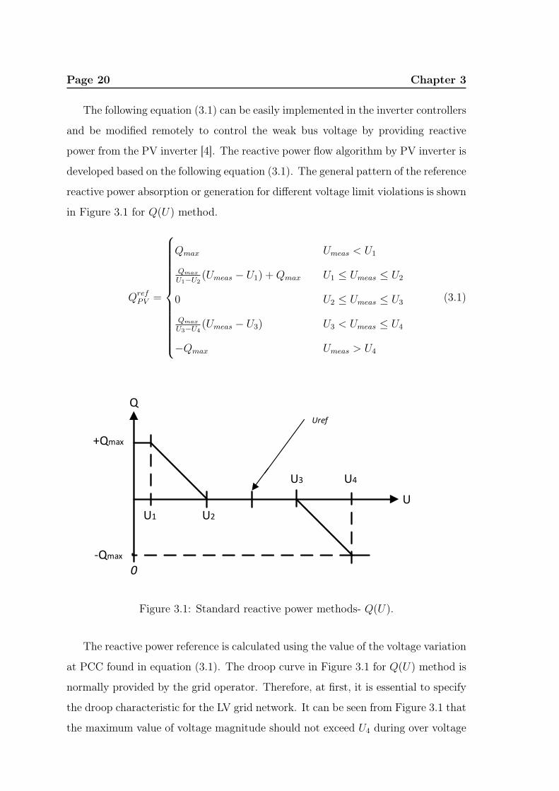
The following equation (3.1) can be easily implemented in the inverter controllers
and be modified remotely to control the weak bus voltage by providing reactive
power from the PV inverter [4]. The reactive power flow algorithm by PV inverter is
developed based on the following equation (3.1). The general pattern of the reference
reactive power absorption or generation for different voltage limit violations is shown
in Figure 3.1 for Q(U) method.
QrefPV =
Qmax Umeas < U1
Qmax
U1−U2(Umeas − U1) +Qmax U1 ≤ Umeas ≤ U2
0 U2 ≤ Umeas ≤ U3
Qmax
U3−U4(Umeas − U3) U3 < Umeas ≤ U4
−Qmax Umeas > U4
(3.1)
U
0
Q
U1 U2
U3 U4
+Qmax
-Qmax
Uref
Figure 3.1: Standard reactive power methods- Q(U).
The reactive power reference is calculated using the value of the voltage variation
at PCC found in equation (3.1). The droop curve in Figure 3.1 for Q(U) method is
normally provided by the grid operator. Therefore, at first, it is essential to specify
the droop characteristic for the LV grid network. It can be seen from Figure 3.1 that
the maximum value of voltage magnitude should not exceed U4 during over voltage

3.1 PV inverter control method - Q(U) Page 21
and at that moment the reactive power absorption is −Qmax. On the other hand,
the minimum value of voltage magnitude should not drop below U1 during under
voltage and at that point the reactive power generation is +Qmax.
The start value for absorbing and generating the reactive power is chosen to be
U3 and U2. Thereafter, the droop characteristics can be formed as Figure 3.1. The
chosen values for the voltages [U1 U2 U3 U4] are provided in the next chapter in
Table 4.1 and Table 4.3 respectively for summer and winter days. The equation for
maximum reactive power is defined by
Qmax = tan(acos(cosϕ))× Pn (3.2)
in which Pn is the nominal PV power production capacity. The nominal active and
maximum reactive power production capacity for the PVs are given in the appendix
section A. The maximum reactive power is provided by PV inverter at power factor
0.85.
Start
Calculateload flow
Read bus voltages
U2≤Umeas≤U3 ?
Calculate Qiref
according to equation (3.1)
Read bus voltages
U≤UlimitQi,PVref =0
Assign PI,PVref value and
QI,PVref =0
No Yes No
Yes
Calculateload flow
Stop
Read bus voltages
Next hour ?No
Yes
Assign Qi,PV
ref
Figure 3.2: Flow chart with the implementation of the Q(U) method.
The flow chart shown in Figure 3.2 presents the implementation of the Q(U)
method for PV inverter. For this purpose the Matlab/Simulink software was used
Page 22 Chapter 3
for load flow analysis based on Newton-Raphson method. During each iteration two
load flow analysis are performed. The effect of active power generation from the PV
plant on the voltage magnitude is investigated initially. Then the reactive power
QrefPV is assigned individually from each PV based on the measured voltage value
Umeas, and a new load flow analysis is performed in order to check if the problem
has been mitigated.
3.2 STATCOM control method
It is already known from the previous chapter that the STATCOM can be designed
to control the required amount of reactive power flow at the bus where it is con-
nected to. Therefore, the control of reactive power flow and direction of flow from
the STATCOM is controlled by the voltage difference between STATCOM output
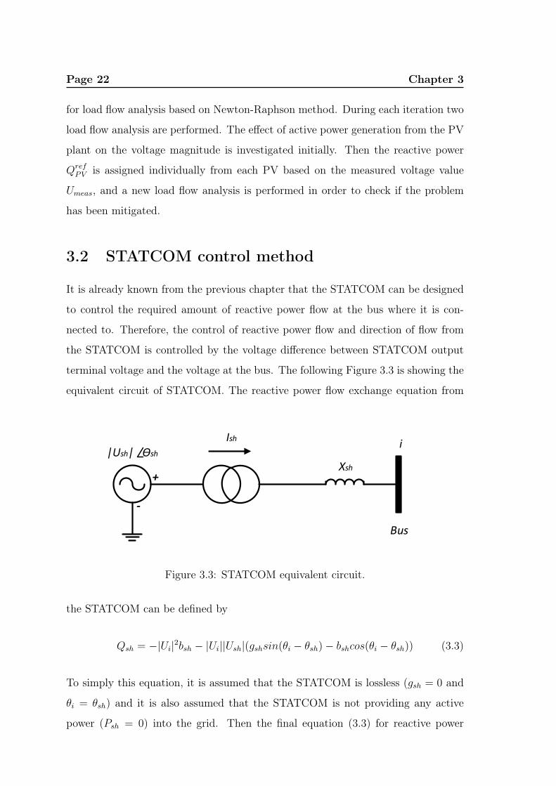
terminal voltage and the voltage at the bus. The following Figure 3.3 is showing the
equivalent circuit of STATCOM. The reactive power flow exchange equation from
Xsh
i
+
-
|Ush| Ѳsh
Bus
Ish
Figure 3.3: STATCOM equivalent circuit.
the STATCOM can be defined by
Qsh = −|Ui|2bsh − |Ui||Ush|(gshsin(θi − θsh)− bshcos(θi − θsh)) (3.3)
To simply this equation, it is assumed that the STATCOM is lossless (gsh = 0 and
θi = θsh) and it is also assumed that the STATCOM is not providing any active
power (Psh = 0) into the grid. Then the final equation (3.3) for reactive power
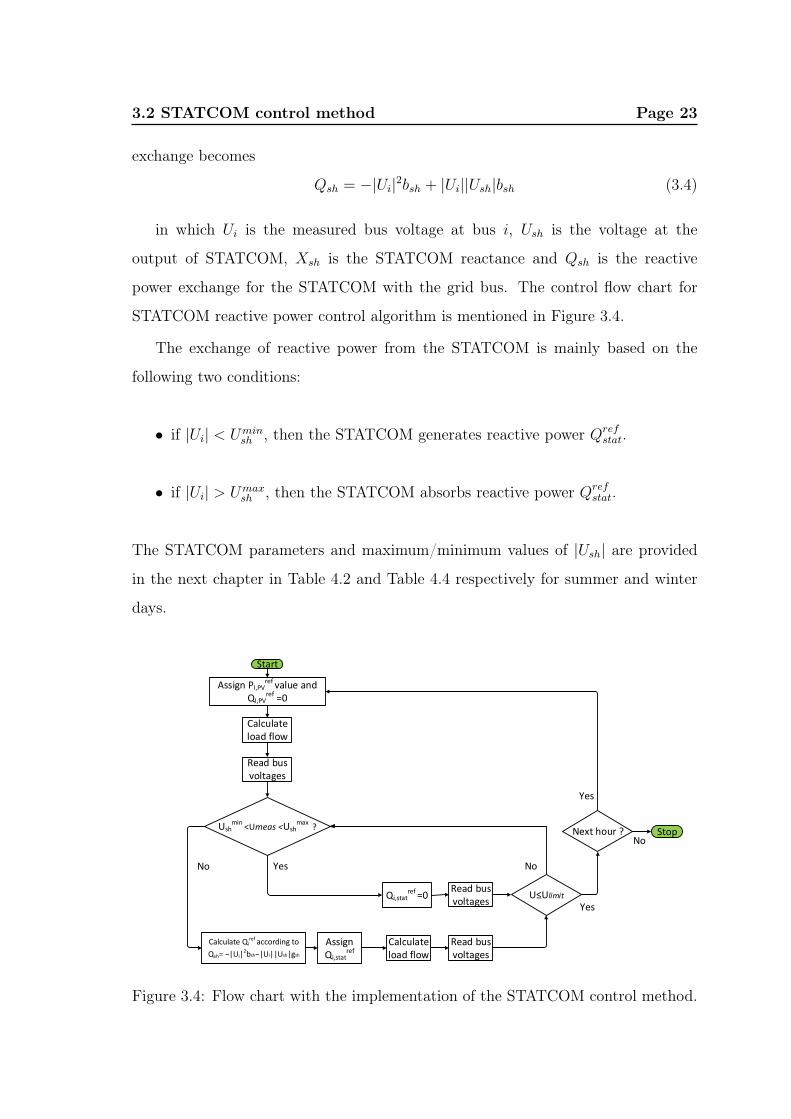
3.2 STATCOM control method Page 23
exchange becomes
Qsh = −|Ui|2bsh + |Ui||Ush|bsh (3.4)
in which Ui is the measured bus voltage at bus i, Ush is the voltage at the
output of STATCOM, Xsh is the STATCOM reactance and Qsh is the reactive
power exchange for the STATCOM with the grid bus. The control flow chart for
STATCOM reactive power control algorithm is mentioned in Figure 3.4.
The exchange of reactive power from the STATCOM is mainly based on the
following two conditions:
• if |Ui| < Uminsh , then the STATCOM generates reactive power Qref
stat.
• if |Ui| > Umaxsh , then the STATCOM absorbs reactive power Qref
stat.
The STATCOM parameters and maximum/minimum values of |Ush| are provided
in the next chapter in Table 4.2 and Table 4.4 respectively for summer and winter
days.
Start
Calculateload flow
Read bus voltages
Ushmin
<Umeas <Ushmax
?
Calculate Qiref according to
Qsh= −|Ui|2bsh−|Ui||Ush|gsh
Read bus voltages
U≤UlimitQi,statref =0
No Yes No
Yes
Calculateload flow
Stop
Read bus voltages
Next hour ?No
Yes
Assign Qi,stat
ref
Assign PI,PVref value and
QI,PVref =0
Figure 3.4: Flow chart with the implementation of the STATCOM control method.
Page 24 Chapter 3
3.3 Proposed coordinated voltage control algorithm
The proposed coordinated voltage control algorithm has been developed for con-
trolling the voltages in the distribution grid. The methods have been developed to
control the grid voltage for two different grid voltage levels: 1) voltage control for
LV grid, and 2) voltage control for both the LV and MV grid together.
3.3.1 Scenario I : Voltage control algorithm for the Low Volt-
age (LV) grid
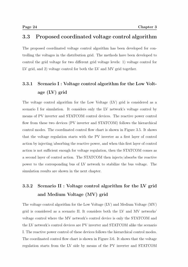
The voltage control algorithm for the Low Voltage (LV) grid is considered as a
scenario I for simulation. It considers only the LV network’s voltage control by
means of PV inverter and STATCOM control devices. The reactive power control
flow from these two devices (PV inverter and STATCOM) follows the hierarchical
control modes. The coordinated control flow chart is shown in Figure 3.5. It shows
that the voltage regulation starts with the PV inverter as a first layer of control
action by injecting/absorbing the reactive power, and when this first layer of control
action is not sufficient enough for voltage regulation, then the STATCOM comes as
a second layer of control action. The STATCOM then injects/absorbs the reactive
power to the corresponding bus of LV network to stabilize the bus voltage. The
simulation results are shown in the next chapter.
3.3.2 Scenario II : Voltage control algorithm for the LV grid
and Medium Voltage (MV) grid
The voltage control algorithm for the Low Voltage (LV) and Medium Voltage (MV)
grid is considered as a scenario II. It considers both the LV and MV networks’
voltage control where the MV network’s control device is only the STATCOM and
the LV network’s control devices are PV inverter and STATCOM alike the scenario
I. The reactive power control of these devices follows the hierarchical control modes.
The coordinated control flow chart is shown in Figure 3.6. It shows that the voltage
regulation starts from the LV side by means of the PV inverter and STATCOM
3.3 Proposed coordinated voltage control algorithm Page 25
Start
Calculateload flow
Read bus voltages
U2≤Umeas≤U3 ?
Calculate Qiref
according to equation (3.1)
Read bus voltages
U≤UlimitAssign
Qi,PVref =0
No Yes No
Yes
Calculateload flow
StopRead bus voltages
Next hour ?No
Yes
Assign Qi,PV
ref
Ushmin
<Umeas <Ushmax
?
Calculate Qiref according to
Qsh= −|Ui|2bsh−|Ui||Ush|gsh
Read bus voltages
U≤UlimitAssign
Qi,statref =0
No Yes No
Yes
Calculateload flow
Read bus voltages
Assign Qi,stat
ref
PV inverter
STATCOM
LV N
etwo
rk con
trol
Assign PI,PVref value and
QI,PVref =0
Figure 3.5: Control flow chart for the Low Voltage (LV) grid.
by injecting/absorbing reactive power into LV network to stabilize the voltage, and
thereafter, the MV control action will take place.
However, it needs to be mentioned that the MV network control action is not that
always the subsequent operation which only occurs after the LV network action. The
MV network control can initiate its control action independently by activating the
STATCOM to stabilize the voltage at the MV nodes. However, if only if there is a
reactive power generation happened in the LV side, then the effect of this generation
will be examined first on the MV grid side and then the MV network control will
take control action depending upon the voltage situation. Otherwise, the LV network
control and MV network control can take their control action independently to bring
the voltage within specified limits. In the next chapter, the simulation and results

Page 26 Chapter 3
are presented with the results analysis.
Start
Calculateload flow
Read bus voltages
U2≤Umeas≤U3 ?
Calculate Qiref
according to equation (3.1)
Read bus voltages
U≤UlimitAssign
Qi,PVref =0
No
Yes
No
Yes
Calculateload flow
Stop
Read bus voltages
Next hour ?No
Yes
Assign Qi,PV
ref
Ushmin
<Umeas <Ushmax
?
Calculate Qiref according to
Qsh= −|Ui|2bsh−|Ui||Ush|gsh
Read bus voltages
U≤UlimitAssign
Qi,statref =0
NoYes
No
Yes
Calculateload flow
Read bus voltages
Assign Qi,stat
ref
PV inverter
STATCOM
Calculate Qiref according to
Qsh= −|Ui|2bsh−|Ui||Ush|gsh
Read bus voltages
U≤Ulimit
Assign Qi,stat
ref =0
No
Yes
NoYes
Calculateload flow
Read bus voltages
Assign Qi,stat
ref
Calculateload flow
Read bus voltages
Qi,PV+statref
exists ?
Yes
Assign Qi,PV+stat
ref
No
Ushmin
<Umeas <Ushmax
?
LV N
etwo
rk con
trol
MV
Ne
two
rk con
trol
STATCOM
Assign PI,PVref value and
QI,PVref =0
Figure 3.6: Control flow chart for the Low Voltage (LV) and Medium Voltage (MV)grid.
Chapter 4
Simulation and Results
Introduction
This chapter presents the grid simulation and results for two control scenarios I and
II based on the proposed coordinated voltage control algorithm developed in the
previous chapter.
4.1 Grid simulation for scenario I and II
The proposed coordinated voltage control algorithm with the help of reactive power
flow would be tested and simulated on grid for two control scenarios. The two
control areas are mentioned in the following Figure 4.1 and they are:
• Scenario I : Low Voltage (LV) network control
• Scenario II : LV network and Medium Voltage (MV) network control
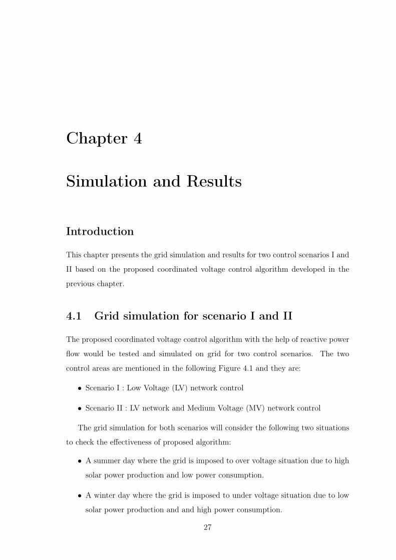
The grid simulation for both scenarios will consider the following two situations
to check the effectiveness of proposed algorithm:
• A summer day where the grid is imposed to over voltage situation due to high
solar power production and low power consumption.
• A winter day where the grid is imposed to under voltage situation due to low
solar power production and and high power consumption.
27
Page 28 Chapter 4
Xi
i
BusbarMV/LVHV/MV
PVLoad PVLoad
1 i+1
Ri
Scenario IScenario II
Figure 4.1: Two control scenarios.
4.1.1 Results for scenario I
The work of this part is programmed with the help of Matlab/Simulink software
for the power flow simulation and simulating the developed reactive power control
method onto control scenario I for the LV grid voltage regulation. As mentioned
before, the proposed control method will be examined for one winter and one summer
day to check the effectiveness of the algorithm.
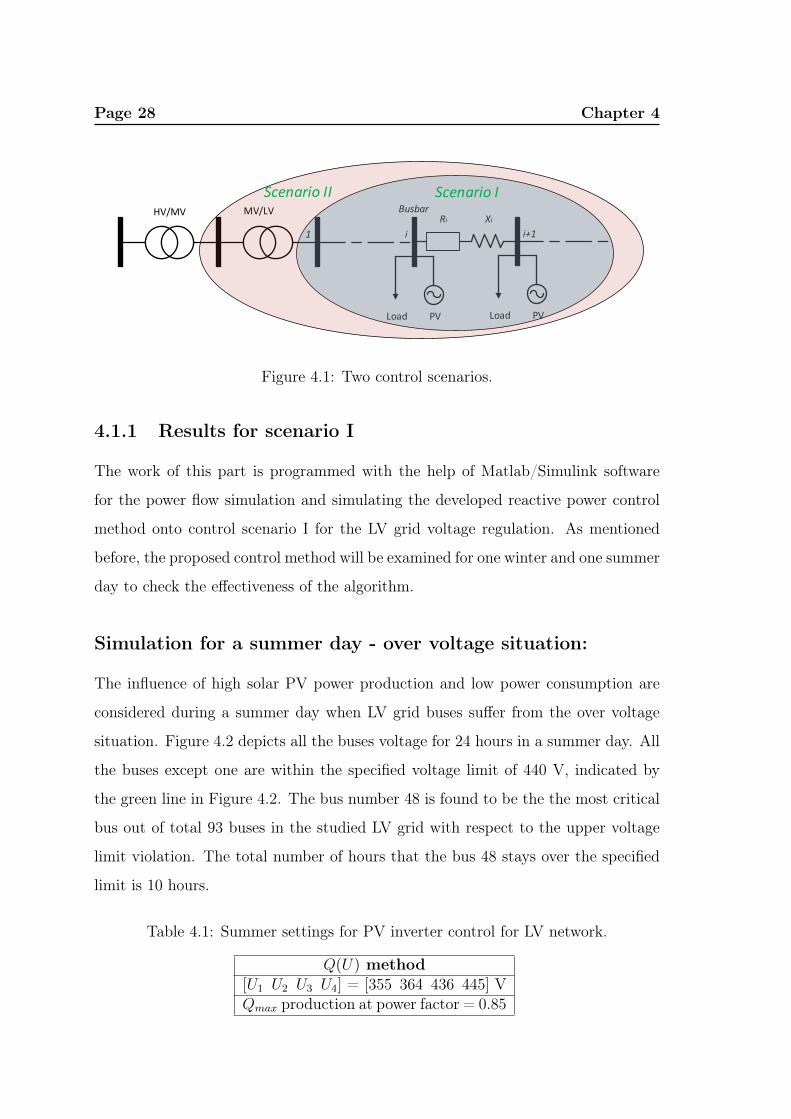
Simulation for a summer day - over voltage situation:
The influence of high solar PV power production and low power consumption are
considered during a summer day when LV grid buses suffer from the over voltage
situation. Figure 4.2 depicts all the buses voltage for 24 hours in a summer day. All
the buses except one are within the specified voltage limit of 440 V, indicated by
the green line in Figure 4.2. The bus number 48 is found to be the the most critical
bus out of total 93 buses in the studied LV grid with respect to the upper voltage
limit violation. The total number of hours that the bus 48 stays over the specified
limit is 10 hours.
Table 4.1: Summer settings for PV inverter control for LV network.
Q(U) method[U1 U2 U3 U4] = [355 364 436 445] VQmax production at power factor = 0.85

4.1 Grid simulation for scenario I and II Page 29
0 10 20 30 40 50 60 70 80 90380
400
420
440
460
480
500
520
Bus
Vo
ltag
e [V
]
Figure 4.2: Voltage in the LV grid buses before applying the voltage control. Totalnumber of buses 93 and each line represents the hourly buses voltage.
The voltage variations of bus 48 at different hours in a day can be seen from
Figure 4.3 where the voltage has crossed the voltage upper limit 440 V due to high
amount of PV power production and low load demand in that bus. So, the voltage
of this bus needs to be controlled in this situation.
0 5 10 15 20380
400
420
440
460
480
500
520
Hours
Vo
ltag
e [V
]
Without control
Controlled by PV inverter
Voltage upper limit
U4
U3
Figure 4.3: Voltage in the critical grid bus 48 after applying the voltage control bythe PV inverter.
To do that, the first control action according to control flow diagram described
in Figure 3.5 will come from the corresponding PV inverter of that bus by absorbing
the reactive power from the grid.

Page 30 Chapter 4
Figure 4.3 depicts that the voltage at the grid bus 48 is reduced by approximately
4.6% for those hours where the bus voltage crossed the upper voltage limit. The PV
inverter connected to bus 48 is absorbing the reactive power to bring the voltage
down and the amount of reactive power absorption is shown in Figure 4.4.
0 5 10 15 20−500
−400
−300
−200
−100
0
Hours
Q [
kV
ar]
Figure 4.4: Reactive power absorption at bus 48 by the PV inverter.
0 10 20 30 40 50 60 70 80 90380
400
420
440
460
480
500
Bus
Vo
ltag
e [V
]
Figure 4.5: Voltage in the grid buses after applying the voltage control by PVinverter. Each line represents the hourly buses voltage.
The voltages for all of the buses after reactive power support by the PV inverter
are shown in Figure 4.5. However, the voltage at the grid bus 48 is still exceeding
the upper voltage limit of 440 V. The PV inverter provides the maximum Q support
4.1 Grid simulation for scenario I and II Page 31
by consuming reactive power that is available at those hours without curtailing any
power; but that is not sufficient enough to bring the voltage down to or below the
upper limit.
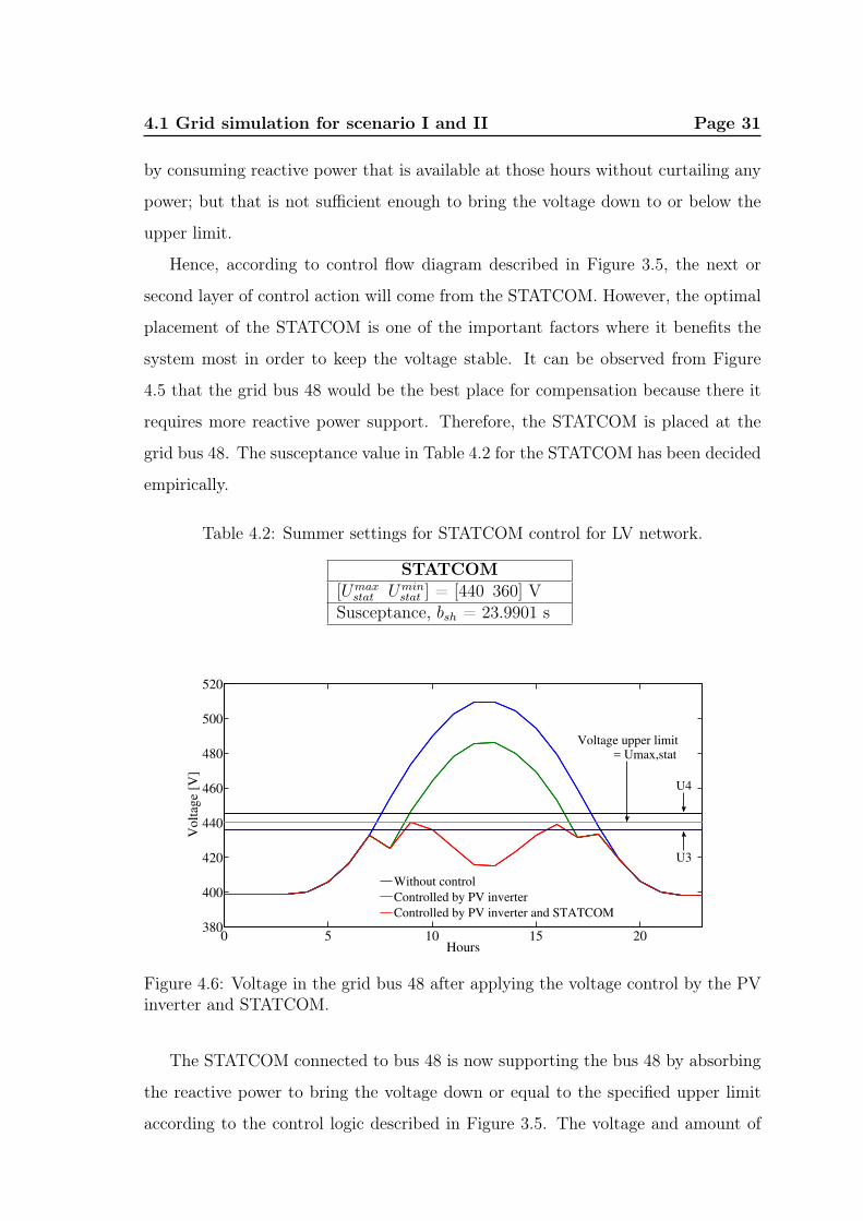
Hence, according to control flow diagram described in Figure 3.5, the next or
second layer of control action will come from the STATCOM. However, the optimal
placement of the STATCOM is one of the important factors where it benefits the
system most in order to keep the voltage stable. It can be observed from Figure
4.5 that the grid bus 48 would be the best place for compensation because there it
requires more reactive power support. Therefore, the STATCOM is placed at the
grid bus 48. The susceptance value in Table 4.2 for the STATCOM has been decided
empirically.
Table 4.2: Summer settings for STATCOM control for LV network.
STATCOM[Umax
stat Uminstat ] = [440 360] V
Susceptance, bsh = 23.9901 s
0 5 10 15 20380
400
420
440
460
480
500
520
Hours
Vo
ltag
e [V
]
Without control
Controlled by PV inverter
Controlled by PV inverter and STATCOM
U3
U4
Voltage upper limit= Umax,stat
Figure 4.6: Voltage in the grid bus 48 after applying the voltage control by the PVinverter and STATCOM.
The STATCOM connected to bus 48 is now supporting the bus 48 by absorbing
the reactive power to bring the voltage down or equal to the specified upper limit
according to the control logic described in Figure 3.5. The voltage and amount of
Page 32 Chapter 4
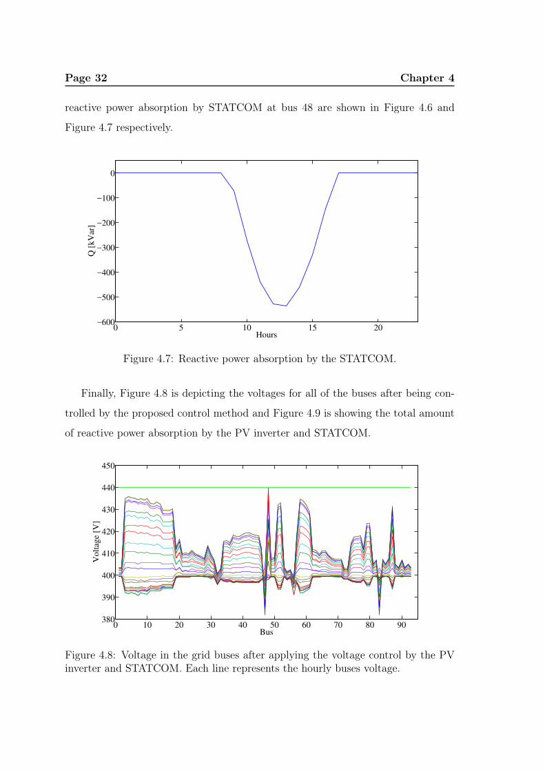
reactive power absorption by STATCOM at bus 48 are shown in Figure 4.6 and
Figure 4.7 respectively.
0 5 10 15 20−600
−500
−400
−300
−200
−100
0
Hours
Q [
kV
ar]
Figure 4.7: Reactive power absorption by the STATCOM.
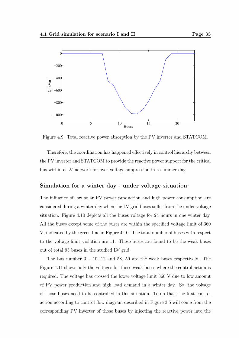
Finally, Figure 4.8 is depicting the voltages for all of the buses after being con-
trolled by the proposed control method and Figure 4.9 is showing the total amount
of reactive power absorption by the PV inverter and STATCOM.
0 10 20 30 40 50 60 70 80 90380
390
400
410
420
430
440
450
Bus
Vo
ltag
e [V
]
Figure 4.8: Voltage in the grid buses after applying the voltage control by the PVinverter and STATCOM. Each line represents the hourly buses voltage.
4.1 Grid simulation for scenario I and II Page 33
0 5 10 15 20
−1000
−800
−600
−400
−200
0
Hours
Q [
kV
ar]
Figure 4.9: Total reactive power absorption by the PV inverter and STATCOM.
Therefore, the coordination has happened effectively in control hierarchy between
the PV inverter and STATCOM to provide the reactive power support for the critical
bus within a LV network for over voltage suppression in a summer day.
Simulation for a winter day - under voltage situation:
The influence of low solar PV power production and high power consumption are
considered during a winter day when the LV grid buses suffer from the under voltage
situation. Figure 4.10 depicts all the buses voltage for 24 hours in one winter day.
All the buses except some of the buses are within the specified voltage limit of 360
V, indicated by the green line in Figure 4.10. The total number of buses with respect
to the voltage limit violation are 11. These buses are found to be the weak buses
out of total 93 buses in the studied LV grid.
The bus number 3 − 10, 12 and 58, 59 are the weak buses respectively. The
Figure 4.11 shows only the voltages for those weak buses where the control action is
required. The voltage has crossed the lower voltage limit 360 V due to low amount
of PV power production and high load demand in a winter day. So, the voltage
of those buses need to be controlled in this situation. To do that, the first control
action according to control flow diagram described in Figure 3.5 will come from the
corresponding PV inverter of those buses by injecting the reactive power into the

Page 34 Chapter 4
0 10 20 30 40 50 60 70 80 90350
360
370
380
390
400
410
Bus
Vo
ltag
e [V
]
Figure 4.10: Voltage at all the grid buses before applying the control. Each linerepresents the hourly buses voltage.
grid. It is important to note that the buses 58 and 59 have no PV system. The total
number of hours that the each weak bus stays below the specified limit are given
below.
• The bus 3 stays for 7 hours
• The bus 4 stays for 7 hours
• The bus 5 stays for 3 hours
• The bus 6 stays for 7 hours
• The bus 7 stays for 9 hours
• The bus 8 stays for 3 hours
• The bus 9 stays for 7 hours
• The bus 10 stays for 7 hours
• The bus 12 stays for 1 hour
• The bus 58 stays for 3 hours
• The bus 59 stays for 3 hours
Table 4.3: Winter settings for PV inverter control for LV network.
Q(U) method[U1 U2 U3 U4] = [355 364 436 445] VQmax production at power factor = 0.85

4.1 Grid simulation for scenario I and II Page 35
0 5 10 15 20350
355
360
365
370
375
380
Hours
Vo
ltag
e [V
]
Bus 3 Bus 4 Bus 5 Bus 6 Bus 7 Bus 8 Bus 9 Bus 10 Bus 12 Bus 58 Bus 59
U2
U1
Voltage lower limit
Figure 4.11: Voltage at all the weak grid buses before applying the voltage control.Each line represents the each bus voltage.
Figure 4.12 shows the voltages at the weak grid buses 3− 10, 12 and 58, 59 and
the voltages are increased for those hours where the bus voltage’s crossed the lower
voltage limit. The PV inverter connected to these buses are injecting the reactive
power into the grid to raise the voltage above the lower voltage limit. The amount
of reactive power injection is shown in Figure 4.13. The voltages for all of the buses
after reactive power support by the PV inverter are shown in Figure 4.14.
0 5 10 15 20350
355
360
365
370
375
380
Hours
Vo
ltag
e [V
]
Bus 3 Bus 4 Bus 5 Bus 6 Bus 7 Bus 8 Bus 9 Bus 10 Bus 12 Bus 58 Bus 59
Voltage lower limit
U2
U1
Figure 4.12: Voltage at all the weak grid buses after applying the voltage control bythe PV inverter. Each line represents the each bus voltage.

Page 36 Chapter 4
0 5 10 15 200
2
4
6
8
10
Hours
Q [
kV
ar]
Bus 3
Bus 4
Bus 5
Bus 6
Bus 7
Bus 8
Bus 9
Bus 10
Bus 12
Figure 4.13: Reactive power injection by the PV inverter.
0 10 20 30 40 50 60 70 80 90350
360
370
380
390
400
410
Bus
Vo
ltag
e [V
]
Figure 4.14: Voltage at all the grid buses after applying the voltage control by PVinverters. Each line represents the hourly buses voltage.
However, the voltage at the weak grid buses are still exceeding the voltage limit
of 360 V. The PV inverters provide the maximum Q support by producing reactive
power that is available at those hours without curtailing any power; even inverters
continue supporting independently when the active/real power generation is zero at
night. The reactive power support at night or during zero real power generation
will be discussed later in this chapter. However, this is not yet sufficient enough to
bring the voltage up to or above the lower limit for all of the weak buses.
4.1 Grid simulation for scenario I and II Page 37
Hence, according to control flow diagram described in Figure 3.5, the next or
second layer of control action will come from the STATCOM. However, the optimal
placement of the STATCOM is one of the important factors where it benefits the
system most in order to keep the voltage stable. It can be observed from Figure 4.14
that the grid buses 7, 9 and 10 require more reactive power support becuase these
three buses have been found to be the weakest buses among the 11 weak buses.
Table 4.4: Winter settings for three STATCOMs’ control for LV network.
STATCOM[Umax
stat Uminstat ] = [440 360] V
Susceptance, bsh = 29.9901 s
Therefore, these three places would be the best place for STATCOM for effective
compensation and voltage regulation. So, three STATCOMs are placed at the LV
grid buses 7, 9 and 10. The susceptance value in Table 4.4 for the STATCOM has
been decided empirically. The three STATCOMs have the identical settings of their
parameters.
0 5 10 15 20350
355
360
365
370
Hours
Vo
ltag
e [V
]
Bus 7
Bus 9
Bus 10
U2
U1
Voltage lower limit=Umin,stat
Figure 4.15: Voltage at the weak grid buses 7, 9 and 10 after applying the voltagecontrol by the PV inverter and STATCOM. Each line represents the each bus voltage.
Now, the STATCOM connected to buses 7, 9 and 10 are now supporting the bus
7, 9 and 10 by injecting the reactive power to bring the voltage up to or equal to the
specified voltage lower limit according to the control logic described in Figure 3.5.

Page 38 Chapter 4
The voltage and amount of reactive power injection by STATCOM at buses 7, 9 and
10 are shown in Figure 4.15 and Figure 4.16 respectively.
0 5 10 15 200
10
20
30
40
50
Hours
Q [
kV
ar]
Bus 7
Bus 9
Bus 10
Figure 4.16: Reactive power generation by the STATCOM.
Finally, Figure 4.17 is depicting the voltages for all of the buses after being
controlled by the proposed control method and Figure 4.18 is showing the total
amount of reactive power injection by the PV inverter and STATCOM.
0 10 20 30 40 50 60 70 80 90
360
365
370
375
380
385
390
395
400
405
Bus
Vo
ltag
e [V
]
Figure 4.17: Voltage at all the grid buses after applying the voltage control by thePV inverter and STATCOM. Each line represents the hourly buses voltage.
4.1 Grid simulation for scenario I and II Page 39
0 5 10 15 200
10
20
30
40
50
Hours
Q [
kV
ar]
Bus 3
Bus 4
Bus 5
Bus 6
Bus 7
Bus 8
Bus 9
Bus 10
Bus 12
Figure 4.18: Total reactive power injection by the PV inverter and STATCOM.
Therefore, the coordination has happened effectively in control hierarchy between
the PV inverter and STATCOM to provide the reactive power support for the critical
bus within a LV network for voltage regulation in a winter day.
4.1.2 Results for scenario II
Due to high or low PV power generation in the LV network, the MV network is also
affected in terms of voltage instability. Additionally, the MV network is affected by
the reactive power generation or absorption in the LV network, and it just happened
in scenario I to control the LV side’s voltage. Now, in terms of impact from these
situations, the MV node’s voltage needs to be examined to check whether the voltage
is within the specified limit according to EN 50160 or not. Depending upon the
voltage at MV node the control action will take place hierarchically which is clearly
shown in Figure 3.6. If the voltage at the MV node violates the specified upper or
lower voltage limit then the MV controller will activate the STATCOM along with
the LV network control system to bring the MV node voltage within allowed limit.
The simulation here will focus only on the MV network control part and LV
network control has already shown in the previous section. The control area is
shown in Figure 4.19. Here, this part will apply the proposed control algorithm
according to Figure 3.6, and the control here is the control of MV node voltage.
Page 40 Chapter 4
This observation is also both for the summer and winter days.
Xi
i
BusbarMV/LVHV/MV
PVLoad PVLoad
1 i+1
Ri
Scenario IScenario II
Figure 4.19: Two control scenarios.
Simulation for a summer day - over voltage situation:
The simulation for a over voltage situation has already been observed and discussed
above, and the LV network was controlled by the PV inverter and STATCOM by
means of reactive power absorption. The following Figure 4.20 is showing the volt-
age at the MV node when no control action was applied at the LV network. The
nominal voltage for the MV node is 10 KV and the voltage magnitude variations
limit according to the EN 50160 is ±10%.
The over voltage limit is for MV node would be 11 KV. It is also observed from
Figure 4.20 that the MV node voltage is already within a upper voltage limit over
the period even when there was no LV network control in action. So, the control
action for MV network’s voltage control is not necessary by means of STATCOM
according to Figure 3.6 as the MV node voltage is within a upper voltage limit over
the period.
However, the voltage at the MV node in Figure 4.20 is slightly affected during
the period when the LV network control came into control action to support the
voltage of LV network buses. It happened because of the reactive power absorption
in the LV network by the PV inverter and STATCOM. Moreover, it is also observed
from Figure 4.20 that the voltage at the MV node got impact positively, and the
direction of the voltage change towards to the nominal voltage 10 KV.

4.1 Grid simulation for scenario I and II Page 41
0 5 10 15 209.98
10
10.02
10.04
10.06
10.08
10.1
Hours
Vo
ltag
e [K
V]
before control
after control
Figure 4.20: Voltage at the MV node before and after the LV network control action.
Simulation for a winter day - under voltage situation:
The simulation for a under voltage situation has already been observed and discussed
above, and the LV network was controlled by the PV inverter and STATCOM by
means of reactive power injection. The following Figure 4.21 is showing the voltage
at the MV node when no control action was applied at the LV network.
The lower voltage limit is for MV node is 9 KV according to grid codes. So,
from Figure 4.21, it is observed that the MV node voltage is already within a lower
voltage limit over the period even when there was no LV network control in action.
So, the control action for MV network’s voltage control is not necessary by means
of STATCOM according to Figure 3.6 as the MV node voltage is within a lower
voltage limit over the period.
However, the voltage at the MV node in Figure 4.21 is slightly affected during
the period when the LV network control came into control action to support the
voltage of LV network. It happened because of the reactive power injection in the
LV network by the PV inverters and STATCOMs. Moreover, it is observed from
Figure 4.21 that the voltage at the MV node got impact positively, and the direction
of the voltage change towards to the nominal voltage 10 KV.

Page 42 Chapter 4
0 5 10 15 209.968
9.97
9.972
9.974
9.976
9.978
9.98
9.982
Hours
Vo
ltag
e [K
V]
before control
after control
Figure 4.21: Voltage at the MV node after the LV network control action.
Nevertheless, if it is required to control the voltage at the MV node, then the
control action will be taking place for controlling the MV node voltage according to
Figure 3.6. In the following paragraph, an additional simulation work is presented
for the MV network’s node voltage control and it considers only the over voltage
situation.
Simulation for 252 MV nodes of the MV network - over voltage
situation:
This section has considered all the 252 nodes of MV network and it will present
the results of control action from the MV network control according to Figure 3.6
for an over voltage situation during one summer day. The parameter settings for
STATCOM is provided in Table 4.5 and decided empirically.
Firstly, one node of the MV network from the Herrljunga municipality distri-
bution network has been presented. Figure 4.22 shows that due to high PV power
production the voltage at the MV node has crossed the specified voltage limit of
11 KV indicated by the red line. Then this over voltage situation is completely
suppressed by the STATCOM control action where the STATCOM absorbed the
reactive power from the grid. The amount of reactive power consumption is shown
in Figure 4.23. It can be observed that the switching of the STATCOM for reactive

4.1 Grid simulation for scenario I and II Page 43
power consumption happened only for an hour and actively supporting the MV node
when the MV node is suffering from the over voltage situation.
Table 4.5: Parameter settings used for STATCOM control during summer for MVnetwork.
STATCOM[Umax
stat Uminstat ] [11 9] KV
Susceptance, bsh 23.9901 s
0 5 10 15 209.8
10
10.2
10.4
10.6
10.8
11
11.2
11.4
Hours
Vo
ltag
e [K
V]
Before control
After control by STATCOM
Voltage upper limit= Umax,stat
Figure 4.22: Voltage at one MV node before and after applying the MV networkcontrol.
0 5 10 15 20−250
−200
−150
−100
−50
0
50
Hours
Q [
kV
ar]
Q absorption by STATCOM
Figure 4.23: Q absorption by the STATCOM at one MV node.

Page 44 Chapter 4
Secondly, the voltage at all the 252 nodes of MV network is shown in Figure 4.24
and it shows the voltage for an hour for all the MV nodes before and after applying
the MV network control. The Figure 4.25 shows the corresponding Q absorption by
the STATCOMs.
0 50 100 150 200 25010
10.2
10.4
10.6
10.8
11
11.2
Nodes
Vo
ltag
e [K
V]
Before control After control by STATCOM
Figure 4.24: Voltage at all MV nodes before and after applying the MV networkcontrol.
0 50 100 150 200 250−50
−40
−30
−20
−10
0
10
Nodes
Q [
MV
ar]
Q absorption by STATCOM
Figure 4.25: Q absorption at all MV nodes by the STATCOM.
The results also show that most of the the MV nodes are under specified voltage
limit by the control action of STATCOMs. For some nodes STATCOM control
action is not sufficient enough to suppress this situation, especially when the PV
power production is very high. The nodes 63−65 , 82, 83, 90, 91, 224, and 240−252
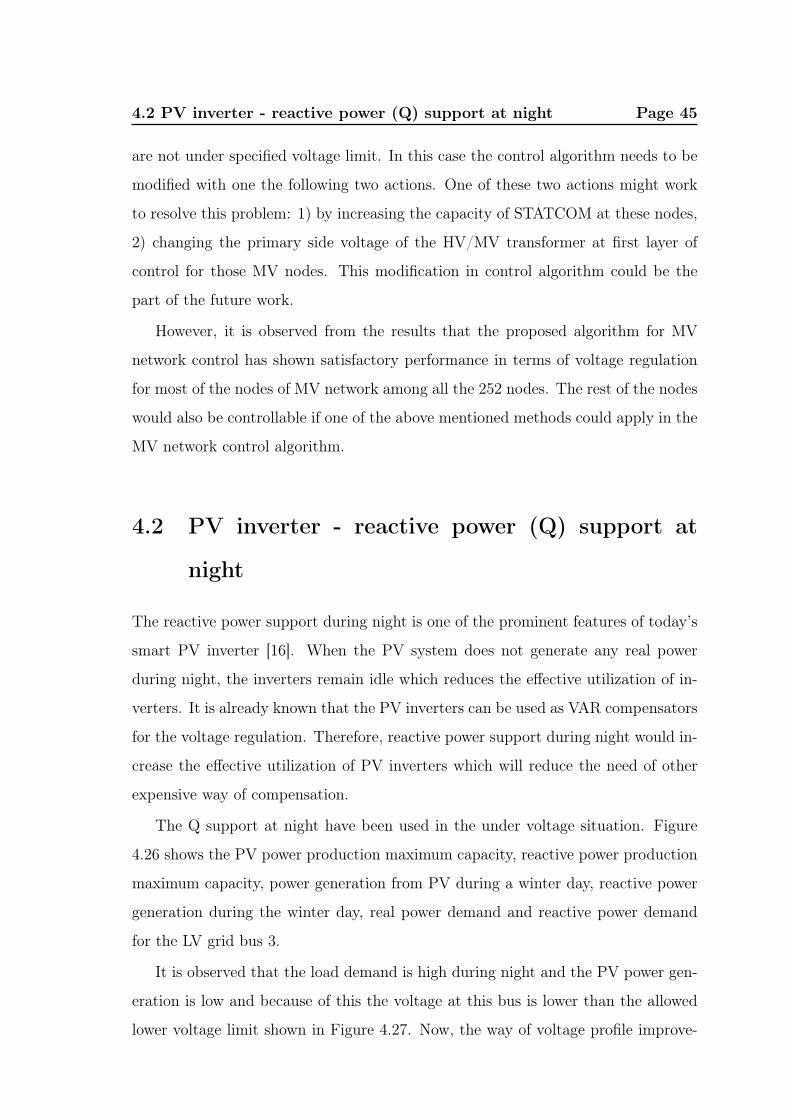
4.2 PV inverter - reactive power (Q) support at night Page 45
are not under specified voltage limit. In this case the control algorithm needs to be
modified with one the following two actions. One of these two actions might work
to resolve this problem: 1) by increasing the capacity of STATCOM at these nodes,
2) changing the primary side voltage of the HV/MV transformer at first layer of
control for those MV nodes. This modification in control algorithm could be the
part of the future work.
However, it is observed from the results that the proposed algorithm for MV
network control has shown satisfactory performance in terms of voltage regulation
for most of the nodes of MV network among all the 252 nodes. The rest of the nodes
would also be controllable if one of the above mentioned methods could apply in the
MV network control algorithm.
4.2 PV inverter - reactive power (Q) support at
night
The reactive power support during night is one of the prominent features of today’s
smart PV inverter [16]. When the PV system does not generate any real power
during night, the inverters remain idle which reduces the effective utilization of in-
verters. It is already known that the PV inverters can be used as VAR compensators
for the voltage regulation. Therefore, reactive power support during night would in-
crease the effective utilization of PV inverters which will reduce the need of other
expensive way of compensation.
The Q support at night have been used in the under voltage situation. Figure
4.26 shows the PV power production maximum capacity, reactive power production
maximum capacity, power generation from PV during a winter day, reactive power
generation during the winter day, real power demand and reactive power demand
for the LV grid bus 3.
It is observed that the load demand is high during night and the PV power gen-
eration is low and because of this the voltage at this bus is lower than the allowed
lower voltage limit shown in Figure 4.27. Now, the way of voltage profile improve-

Page 46 Chapter 4
0 5 10 15 20
0
500
1000
1500
2000
2500
3000
Hours
P[W
],
Q[V
ar]
PV power generation [W]
Q generated [Var]
PV max. capacity [W]
Q max. capacity [Var]
P load [W]
Q load [Var]
Figure 4.26: P and Q scenarios for the LV grid bus 3.
ment is through supplying Q power from the PV inverter and it can be observed
from Figure 4.27 that the voltage profile has been improved by approximately 1.2%.
0 5 10 15 20350
355
360
365
370
375
Hours
Vo
ltag
e [V
]
Voltage before Q injection
Voltage after Q injection
U2
Voltage lower limit
U1
Figure 4.27: Voltage at the LV grid bus 3 before and after Q compensation by thePV inverter.
So, the bus voltage is completely under allowed voltage limit through the reactive
power compensation technique, and by utilizing only the PV inverter’s available Q
capacity during night. Finally, the appendix section A.2 will collectively present the
summary on seasonal parameter settings for both the PV inverter and STATCOM.
Additionally, the appendix section A.3 will provide the details on the PV systems
data that have been used throughout the simulation.
Chapter 5
Discussion
This chapter provides an overall discussion on methodology, input data, system
effects due to high PV power production, compensation techniques to overcome the
effects.
5.1 Methodology and input data
Voltage management by means of reactive power compensation with the accurate
reactive power control model can be used to fulfill the grid codes in distribution
grids with a large PV penetration. Therefore, in this thesis work, the reactive power
control for voltage stability has been considered by proposing effective coordinated
voltage control methods.
The used methods for coordinated voltage control have two layers of control
actions. The first layer of control action used in this thesis is directly provided by
the PV inverter with a Q(U) voltage control method. Thereafter, the second layer of
control action is provided by the STATCOM based on voltage droop characteristics.
The control model for the PV inverter, STATCOM, coordinated reactive power
control method and load flow model are implemented in a house built program in
Matlab/Simulink that enables to design, modify and analyze the control model to
fit the specific grid requirements.
The coordinated control method has been tested upon for two scenarios where
seasonal variations of PV power and load demand are considered. The control47

Page 48 Chapter 5
response in terms of voltage stability for both winter and summer from the proposed
coordinated voltage control method has shown the potential use of both the control
algorithm and combination of PV inverter and STATCOM. However, the criteria to
use this method requires accurate settings of PV inverter and STATCOM control
parameters. It is one of the observations that one setting for one LV network and one
MV node does not work for other networks or nodes, especially for those networks
or nodes where PV power production is very high.
It is also observed that the networks suffering most in terms of voltage instability
due to very high PV power production requires modification of proposed control
algorithms. However, I had applied the developed LV network control algorithm
for some other LV networks as well which are under different MV nodes to check
the generality of the developed algorithm. It is observed from the simulation that
for some LV networks the voltage profile collapsed especially for those LV networks
where all the LV grid buses are extremely violating the voltage limit. On the other
hand, the proposed algorithm worked for some other LV voltage networks where not
every LV grid buses are violating the voltage limit or the violation is not extreme.
So, I only presented the simulation results in this thesis for one LV network out of
other LV networks that worked. It is obvious from the simulation results that the
proposed algorithm is applicable for specific grid structure and situation.
Nevertheless, to generalize the developed algorithm for the other LV networks,
it requires modification in the proposed algorithm. The modification in control
flow algorithm demands that the first layer of control action should come from the
MV distribution side by changing the primary voltage of MV/LV transformer (node
voltage of MV) and thereafter, the second layer of control action would be provided
by the LV network control as presented in Figure 3.5.
This is also true for controlling the voltage of 252 nodes of MV network. The first
layer of control action should control the primary voltage of HV/MV transformer
and then the second layer of control action will be activated by the MV network
control as presented in Figure 3.6. However, other solutions might include power
curtailment, peak shaving by the energy storage or distribution line reinforcement.
In the simulation the input data for the reactive power load demand has been
5.2 System effects and compensation techniques Page 49
produced from the available real active power demand of the Swedish municipality
of Herrljunga by assuming that all the loads are operating at 0.95 power factor. It
would probably be more realistic if the real reactive power load demand was found.
However, it was not a big problem from technical point of view for control method
designing. The data for each PV inverter maximum capacity was determined by
taking the day of the maximum generation in a year.
5.2 System effects and compensation techniques
The fast growing penetration PV power into the distribution grid is a present and
future scenario in the energy system. But the system effects from the variable
nature of PV power production is the challenge in terms of voltage stability to
the distribution grid operators, although it is not the case for Sweden yet. In this
study the reactive power support by two compensation devices (PV inverters and
STATCOM) has been considered to overcome this voltage instability issues.
The main advantage of using the PV inverter as a way of first control implies
that the grid system can be benefited technically by importing/exporting instant
reactive power locally from the cheap and already existing PV inverter than installing
expensive way of other compensation devices. Moreover, the results show that even
if the PV system does not produce any real power, the PV inverter still yields
the reactive power during night for voltage regulation. Thereafter, the STATCOM
has shown the benefit to remove the voltage instability from the weakest buses by
providing reactive power.
Therefore, in combination with the PV inverter and STATCOM, and their coor-
dinated control have presented the effective way of voltage regulation for both the
over- and undervoltage situations.

Page 50 Chapter 5
Chapter 6
Conclusion and Future Work
This chapter highlights the main conclusions of the study presented in this thesis
and summarizes the ideas for future research work.
6.1 Conclusion
This thesis has been an attempt to address the importance of reactive power com-
pensation for large scale PV systems integration into power distribution grids. In
this regard, the role and impact of having PV inverter and STATCOM for reactive
power compensation are analyzed with the chosen grid codes. The voltage profile
control in a distribution grid - via the reactive power contribution of PV inverter
and STATCOM- is based on the indirect voltage control when the reactive power
regulation is direct.
The overall conclusions of this thesis are (i) the proposed approach efficiently
regulates the bus voltages of LV and MV networks to the steady-state voltage limit
according to the grid codes for both the over- and undervoltage situations, (ii) the
STATCOM, coupled with the existing PV inverter, has shown both the reliability for
effective reactive power compensation as well as the potential of ensuring compliance
with the grid codes in terms of voltage stability, (iii) results from the simulation
indicated that the Q supply from PV inverter at night can efficiently be utilized for
the grid voltage stability, and (iv) the proposed algorithm has shown satisfactory
performance in terms of voltage regulation.51

Page 52 Chapter 6
6.2 Future work
As future work, a number of points can be paid attention to, in order to further
demonstrate the benefits of STATCOM and PV inverter devices in grid voltage
management. The future work might include the following points:
• Different PV inverter control strategies such as Q(P ) and Q(P,U) methods
can be examined and compared with the used Q(U) mehtod in this thesis.
• Voltage control algorithm might be extended to adapt the other grid networks
as well.
• Including an energy storage in the algorithm to shape the peak power during
high PV power generation.
• The economical analysis would be interesting for the feasibility analysis.

Chapter 7
Acknowledgements
This thesis is the product of my research carried out during master’s studies. This
work was accomplished with the help and support of several people.
Firstly, I would like to express my most sincere gratitude to my supervisor, Mr.
Rasmus Luthander for his investment of time, patience, and effort in my work. His
patient guidance, encouragement and advices that he provided throughout my thesis
work was the key in achieving this thesis.
I am also grateful to Dr. Joakim Widén and Dr. Juan de Santiago for providing
me with valuable advices during meetings.
I would like to thank my friend Joel to be my opponent. I am also grateful to
my corridor friend at Flogsta, Sandrine Lemaire Hamel, for the time she dedicated
to edit the most important part of this thesis.
I am also thankful to the Division of Solid State Physics for providing me a very
friendly work environment, and of course nice coffee breaks.
Finally, thanks to the Uppsala University, that allowed me to come to Sweden
and pursue a master’s degree.
MD. Shakib Hasan
53

Page 54 Chapter 7
Bibliography
[1] Benot Bletterie, Serdar Kadam, Roman Bolgaryn, and Antony Zegers. Voltage
Control with PV Inverters in Low Voltage Networks—In Depth Analysis of
Different Concepts and Parameterization Criteria. IEEE TRANSACTIONS
ON POWER SYSTEMS, 32(1), 2017. doi: 10.1109/TPWRS.2016.2554099.
[2] Jesus Garcia Benito and Rocio Hoya Arija. An alternative Volt / VAR man-
agement scheme for Active Distribution Grids. Technical report, 2014.
[3] Afshin Samadi. Large Scale Solar Power Integration in Distribution Grids Large
Scale Solar Power Integration in Distribution Grids. Technical report, 2014.
[4] Erhan Demirok, Pablo Casado González, Kenn H B Frederiksen, Dezso Sera,
Pedro Rodriguez, and Remus Teodorescu. Local reactive power control meth-
ods for overvoltage prevention of distributed solar inverters in low-voltage grids.
IEEE Journal of Photovoltaics, 1(2):174–182, 2011. ISSN 21563381. doi:
10.1109/JPHOTOV.2011.2174821.
[5] Voltage Regulators - Siemens. URL https://www.energy.siemens.com/hq
/en/power-transmission/transformers/distribution-transformers/
distribution/voltage-regulators.htm.
[6] Ioulia T. Papaioannou, Arturs Purvins, and Charis S. Demoulias. Reactive
power consumption in photovoltaic inverters: a novel configuration for voltage
regulation in low-voltage radial feeders with no need for central control. Progress
in Photovoltaics: Research and Applications, 23(5):611–619, 2015. ISSN 1099-
159X. doi: 10.1002/pip.2477. URL http://dx.doi.org/10.1002/pip.2477.
PIP-12-059.R1.55
Page 56 BIBLIOGRAPHY
[7] Anders Hagehaugen. Voltage Control in Distribution Network with Local Gen-
eration. Technical Report June, 2014.
[8] Alfred Einfalt, Franz Zeilinger, Roman Schwalbe, Benoit Bletterie, and Ser-
dar Kadam. Controlling active low voltage distribution grids with min-
imum efforts on costs and engineering. IECON Proceedings (Industrial
Electronics Conference), pages 7456–7461, 2013. ISSN 1553-572X. doi:
10.1109/IECON.2013.6700374.
[9] Novalio Daratha, Biswarup Das, and Jaydev Sharma. Coordination between
OLTC and SVC for voltage regulation in unbalanced distribution system dis-
tributed generation. IEEE Transactions on Power Systems, 29(1):289–299,
2014. ISSN 08858950. doi: 10.1109/TPWRS.2013.2280022.
[10] Ishtiaq Ahmad, Peter Palensky, and Wolfgang Gawlik. Multi-Agent System
based Voltage Support by Distributed Generation in Smart Distribution Net-
work. pages 329–334, 2015. doi: 10.1109/SEDST.2015.7315230.
[11] Mana Farrokhseresht. Reactive Power Planning with Voltage Stability Con-
straints for Increasing Cross-Border Transmission Capacity. Technical report,
2015.
[12] Elena Anamaria Man. Control of Grid Connected PV Systems with Grid Sup-
port Functions. Technical report, 2011-2012.
[13] Jingsheng HUANG, Meiying LIU, Junjun ZHANG, Wei DONG, and Zhilei
CHEN. Analysis and field test on reactive capability of photovoltaic power
plants based on clusters of inverters. Journal of Modern Power Systems and
Clean Energy, 5(2):283–289, 2015. ISSN 2196-5625. doi: 10.1007/s40565-015-
0154-7. URL http://link.springer.com/10.1007/s40565-015-0154-7.
[14] Miguel JUAMPEREZ, Guangya YANG, and Søren Bækhøj KJÆR. Voltage reg-
ulation in LV grids by coordinated volt-var control strategies. Journal of Modern
Power Systems and Clean Energy, 2014. ISSN 21965420. doi: 10.1007/s40565-
014-0072-0.
BIBLIOGRAPHY Page 57
[15] Piotr Lipnicki and Tiberiu Mihai Stanciu. Reactive power control for Wind
Power Plant with STATCOM. Technical report, 2010.
[16] Q at Night - SMA. URL files.sma.de/dl/18858/Q-at-Night-TI-en-11.pdf.

Page 58 BIBLIOGRAPHY

Appendix A
System data
A.1 Grid code data
Table A.1: Allowed voltage limit in steady-state for both MV and LV network.
EN 50160 standardNominal voltage 10 KV 400 VVoltage upper limit 11 KV 440 VVoltage lower limit 9 KV 360 V
A.2 Summary on parameter settings for compen-
sators
Table A.2: Parameter settings used seasonally for PV inverters and STATCOMs forLV and MV network control.
Compensator Parameter Season LV MV
Summer 23.9901 s 23.9901 s
STATCOMSusceptance, bsh Winter 29.9901 s -
Summer [440 360] V [11 9] KV[Umax
stat Uminstat ] Winter [440 360] V -
Summer 0.85 -
PV inverterPower factor, cosϕ up to
Winter 0.85 -
Summer [355 364 436 445] V -[U1 U2 U3 U4] Winter [355 364 436 445] V -
59

Page 60 Chapter A
A.3 PV system data
Bus
Number
Pmax
(W)
Qmax
(Var)
Bus
Number
Pmax
(W)
Qmax
(Var)
Bus
Number
Pmax
(W)
Qmax
(Var)
1 0 0 41 8738,293 6553,719 81 0 0
2 0 0 42 6955,882 5216,912 82 0 0
3* 2990,727 2243,045 43 12672,85 9504,639 83 0 0
4* 9578,797 7184,098 44 6015,167 4511,375 84 0 0
5* 6691,194 5018,395 45 5036,784 3777,588 85 0 0
6* 5263,625 3947,718 46 4084,398 3063,299 86 0 0
7* 5872,86 4404,645 47 0 0 87 0 0
8* 12421,71 9316,285 48* 451782,7 602376,9 88 0 0
9* 4210,452 3157,839 49 4943,407 3707,555 89 0 0
10* 8522,583 6391,937 50 3751,718 2813,789 90 0 0
11 10920,91 8190,684 51 5928,865 4446,649 91 0 0
12* 6163,453 4622,59 52 14322,79 10742,1 92 0 0
13 12137,74 9103,305 53 0 0 93 0 0
14 9955,438 7466,578 54 0 0
15 13727,8 10295,85 55 0 0
16 9757,248 7317,936 56 4953,351 3715,013
17 4976,019 3732,014 57 0 0
18 12958,84 9719,127 58* 0 0
19 6637,538 4978,154 59* 0 0
20 34356,46 25767,35 60 0 0
21 18290,68 13718,01 61 0 0
22 4480,077 3360,058 62 0 0
23 15355,16 11516,37 63 0 0
24 55659,98 41744,99 64 0 0
25 19103,47 14327,6 65 0 0
26 0 0 66 0 0
27 9174,322 6880,741 67 0 0
28 0 0 68 0 0
29 62467,37 46850,53 69 0 0
30 7085,456 5314,092 70 0 0
31 0 0 71 0 0
32 0 0 72 0 0
33 7462,985 5597,239 73 0 0
34 5859,827 4394,87 74 0 0
35 5301,891 3976,418 75 0 0
36 6073,256 4554,942 76 0 0
37 10679,66 8009,746 77 0 0
38 4824,822 3618,616 78 0 0
39 5286,696 3965,022 79 0 0
40 7341,678 5506,259 80 0 0
The buses containing Pmax and Qmax values are the PV connected buses.
Pmax = PV nominal power capacity
Qmax = PV maximum reactive power generation capacity
‘*’ = The weak and critical buses
Figure A.1: PV systems’ P and Q capacity information.


