QUASARS, CARBON, AND SUPERNOVAE:
EXPLORING THE DISTRIBUTION OF ELEMENTS
IN AN EXPANDING UNIVERSE
by
Shailendra Kumar Vikas
Bachelor of Technology, Indian Institute of Technology, Kharagpur,
2001
Master of Science, University of Pittsburgh, 2007
Submitted to the Graduate Faculty of
the Department of Physics and Astronomy in partial fulfillment
of the requirements for the degree of
Doctor of Philosophy
University of Pittsburgh
2013

UNIVERSITY OF PITTSBURGH
DEPARTMENT OF PHYSICS AND ASTRONOMY
This dissertation was presented
by
Shailendra Kumar Vikas
It was defended on
Aug 10, 2012
and approved by
W. Michael Wood-Vasey
Jeffery Newman
Andrew R. Zentner
Vittorio Paolone
Rupert Croft
Dissertation Director: W. Michael Wood-Vasey
ii

Copyright c© by Shailendra Kumar Vikas
2013
iii
QUASARS, CARBON, AND SUPERNOVAE: EXPLORING THE
DISTRIBUTION OF ELEMENTS IN AN EXPANDING UNIVERSE
Shailendra Kumar Vikas, PhD
University of Pittsburgh, 2013
This thesis consists of three different studies with a common goal of understanding the
constituents and structures of the universe.
The current understanding of galaxy formation is not complete. Cold and hot flows in
galaxies play a role in the evolution and transportation of elements within halos. Ionized
carbon clouds are often observed in the spectra of back-lighting quasars. I study the clus-
tering properties of the triply ionized carbon clouds from SDSS-III data to determine the
minimum mass of the host halo in which galaxy formation processes produce such clouds.
Apart from enabling better understanding of these clouds, this result will help constrain
galaxy formation theory and the associated feedback processes.
Standard cosmological theory produces an excess of baryonic structure compared to the
observed one. Energetic quasars are often envisaged as the process which injects kinetic
energy into the structures and halts the structure formation. I study the outflow in SDSS-
III quasars through the observed velocities of the triply ionized carbon clouds detected in
their spectra. Using more accurate modeling of the abundance of carbon clouds, I make
robust conclusions about properties of outflow systems. Understanding the velocities of such
outflow helps constrain the amount of energy injected in the feedback process of quasars and
helps in explaining the observed baryonic structure of the Universe.
Supernovae Ia enable us to measure distances at different redshifts. Distances enable us
to infer the expansion history of the Universe and measure the current accelerated expansion.
The equation-of-state parameter, w, of the dark energy responsible for this acceleration, can
iv

be determined from the expansion history. I estimate w using data from ESSENCE and other
current supernova surveys and measure the effect of the important systematic uncertainties
that are expected to have the largest contribution to the uncertainty in our understanding
of dark energy.
v

TABLE OF CONTENTS
PREFACE . . . . . . . . . . . . . . . . . . . . . . . . . . . . . . . . . . . . . . . . . xii
1.0 INTRODUCTION . . . . . . . . . . . . . . . . . . . . . . . . . . . . . . . . . 1
1.1 Early Universe . . . . . . . . . . . . . . . . . . . . . . . . . . . . . . . . . 2
1.2 Structure Formation . . . . . . . . . . . . . . . . . . . . . . . . . . . . . . 3
1.3 Quasars . . . . . . . . . . . . . . . . . . . . . . . . . . . . . . . . . . . . . 6
1.3.1 Discovery and Basic Nature of Quasars . . . . . . . . . . . . . . . . 7
1.3.2 Unified Quasar structure . . . . . . . . . . . . . . . . . . . . . . . . 8
1.3.3 Quasar Properties . . . . . . . . . . . . . . . . . . . . . . . . . . . 10
1.3.4 Significance of Quasars for cosmology . . . . . . . . . . . . . . . . . 11
1.3.5 Understanding the origin of quasar absorption systems . . . . . . . 12
1.3.6 Understanding Quasars using absorption lines . . . . . . . . . . . . 13
1.4 Supernova . . . . . . . . . . . . . . . . . . . . . . . . . . . . . . . . . . . . 13
1.4.1 Supernovae Ia and Properties . . . . . . . . . . . . . . . . . . . . . 15
1.4.2 Progenitors of Supernova Ia . . . . . . . . . . . . . . . . . . . . . . 17
2.0 C IV ABSORBER-QUASAR CROSS CORRELATION . . . . . . . . . . 22
2.1 Absorption Systems . . . . . . . . . . . . . . . . . . . . . . . . . . . . . . . 22
2.2 Large scale clustering . . . . . . . . . . . . . . . . . . . . . . . . . . . . . . 24
2.3 Motivation . . . . . . . . . . . . . . . . . . . . . . . . . . . . . . . . . . . . 26
2.4 Data . . . . . . . . . . . . . . . . . . . . . . . . . . . . . . . . . . . . . . . 29
2.4.1 BOSS . . . . . . . . . . . . . . . . . . . . . . . . . . . . . . . . . . 29
2.4.2 Quasars . . . . . . . . . . . . . . . . . . . . . . . . . . . . . . . . . 29
2.4.3 Random Catalog for Quasars . . . . . . . . . . . . . . . . . . . . . 30
vi

2.4.4 C IV Absorption line identification pipeline . . . . . . . . . . . . . . 32
2.4.5 The C IV sample . . . . . . . . . . . . . . . . . . . . . . . . . . . . 33
2.5 Correlation Analysis . . . . . . . . . . . . . . . . . . . . . . . . . . . . . . 36
2.5.1 Error Estimation . . . . . . . . . . . . . . . . . . . . . . . . . . . . 40
2.5.2 Fitting for the Correlation Function and Bias . . . . . . . . . . . . 41
2.6 Results . . . . . . . . . . . . . . . . . . . . . . . . . . . . . . . . . . . . . . 42
2.6.1 Cross Correlation of C IV absorbers and quasars . . . . . . . . . . . 42
2.6.2 Cross-Correlation at large distance . . . . . . . . . . . . . . . . . . 43
2.6.3 Estimation of C IV bias . . . . . . . . . . . . . . . . . . . . . . . . . 43
2.6.4 Comparison with previous results . . . . . . . . . . . . . . . . . . . 50
2.7 Systematic Uncertainties . . . . . . . . . . . . . . . . . . . . . . . . . . . . 52
2.7.1 North Galactic Cap vs Full Sample . . . . . . . . . . . . . . . . . . 52
2.7.2 CORE vs BONUS Systematics Error . . . . . . . . . . . . . . . . . 56
2.7.3 Measurement Robust Across Different BOSS Chunks . . . . . . . . 56
2.7.4 Other Systematic Errors . . . . . . . . . . . . . . . . . . . . . . . . 58
2.8 Summary and Future Directions . . . . . . . . . . . . . . . . . . . . . . . . 67
3.0 QUASAR OUTFLOWS USING INTRINSIC ABSORPTION SYSTEMS 69
3.1 Motivation . . . . . . . . . . . . . . . . . . . . . . . . . . . . . . . . . . . . 69
3.2 Number Density of C IV absorbers . . . . . . . . . . . . . . . . . . . . . . . 71
3.3 Correlation Functions in a Halo Model Framework . . . . . . . . . . . . . . 73
3.3.1 Basics of The Halo Model Formalism . . . . . . . . . . . . . . . . . 74
3.3.2 Mass Function and Bias . . . . . . . . . . . . . . . . . . . . . . . . 76
3.3.3 Density profiles of Halos . . . . . . . . . . . . . . . . . . . . . . . . 77
3.4 Data . . . . . . . . . . . . . . . . . . . . . . . . . . . . . . . . . . . . . . . 78
3.5 Estimation of the cross-correlation function . . . . . . . . . . . . . . . . . . 85
3.6 Results . . . . . . . . . . . . . . . . . . . . . . . . . . . . . . . . . . . . . . 89
3.6.1 Estimation of parameters for the full dataset . . . . . . . . . . . . . 90
3.6.2 Luminosity Dependence for Outflow . . . . . . . . . . . . . . . . . 90
3.6.3 Outflowing absorber properties . . . . . . . . . . . . . . . . . . . . 98
3.6.3.1 FWHM of outflowing absorbers . . . . . . . . . . . . . . . . 98
vii

3.6.3.2 Equivalent width of outflowing absorbers . . . . . . . . . . 100
3.6.4 Comparison with other result . . . . . . . . . . . . . . . . . . . . . 103
3.7 Summary and Future Direction . . . . . . . . . . . . . . . . . . . . . . . . 106
4.0 SUPERNOVA IA COSMOLOGY AND SYSTEMATICS . . . . . . . . . 108
4.1 Cosmology with Supernova Ia . . . . . . . . . . . . . . . . . . . . . . . . . 109
4.2 Dust extinction and the relationship between dust and SN Ia progenitors . 110
4.3 Supernova Data For this Study . . . . . . . . . . . . . . . . . . . . . . . . 111
4.3.1 ESSENCE Supernova Survey . . . . . . . . . . . . . . . . . . . . . 111
4.3.2 Low redshift sample . . . . . . . . . . . . . . . . . . . . . . . . . . 112
4.3.3 Other Surveys . . . . . . . . . . . . . . . . . . . . . . . . . . . . . . 113
4.4 Light Curve Estimator . . . . . . . . . . . . . . . . . . . . . . . . . . . . . 113
4.4.1 SALT II . . . . . . . . . . . . . . . . . . . . . . . . . . . . . . . . . 114
4.5 Monte Carlo Simulation . . . . . . . . . . . . . . . . . . . . . . . . . . . . 115
4.5.1 SNANA . . . . . . . . . . . . . . . . . . . . . . . . . . . . . . . . . 115
4.5.2 Simulation data . . . . . . . . . . . . . . . . . . . . . . . . . . . . . 116
4.6 Systematic Uncertainties of the Supernova Analysis . . . . . . . . . . . . . 117
4.6.1 List of systematic uncertainties . . . . . . . . . . . . . . . . . . . . 117
4.6.2 Methodology . . . . . . . . . . . . . . . . . . . . . . . . . . . . . . 121
4.6.3 Analysis . . . . . . . . . . . . . . . . . . . . . . . . . . . . . . . . . 122
4.7 Conclusion and Future Direction . . . . . . . . . . . . . . . . . . . . . . . 132
5.0 BIBLIOGRAPHY . . . . . . . . . . . . . . . . . . . . . . . . . . . . . . . . . 134
APPENDIX. ABSORPTION PIPELINE . . . . . . . . . . . . . . . . . . . . . 150
A.1 Introduction . . . . . . . . . . . . . . . . . . . . . . . . . . . . . . . . . . . 150
A.2 Shortcoming in Usability of the pipeline . . . . . . . . . . . . . . . . . . . 152
A.3 Improvement in pipeline . . . . . . . . . . . . . . . . . . . . . . . . . . . . 152
A.3.1 What is SWIG? . . . . . . . . . . . . . . . . . . . . . . . . . . . . . 154
A.3.2 Changes for input/output issues. . . . . . . . . . . . . . . . . . . . 154
A.3.3 Other improvements . . . . . . . . . . . . . . . . . . . . . . . . . . 154
viii
LIST OF TABLES
2.1 Table of NCIV for different selection cuts . . . . . . . . . . . . . . . . . . . . 38
2.2 Correlation length and slope of C IV absorbers and quasars. . . . . . . . . . . 47
2.3 Systematic error estimates and p-values for r0, γ and√
bCIVbQSO. . . . . . . 63
2.4 Random error distribution for r0, γ and√
bCIVbQSO. . . . . . . . . . . . . . . 63
3.1 Table of NCIV for different selection cuts . . . . . . . . . . . . . . . . . . . . 80
3.2 Estimated parameters, using halo model formalism. . . . . . . . . . . . . . . 87
3.3 The best-fit parameters of the model for all absorber data. . . . . . . . . . . 94
3.4 The best-fit parameters of the model for all absorber data. . . . . . . . . . . 95
3.5 Individual component as a percent of the total sample. . . . . . . . . . . . . 95
3.6 Velocity of the Outflow . . . . . . . . . . . . . . . . . . . . . . . . . . . . . . 95
4.1 Table of systematic errors on w . . . . . . . . . . . . . . . . . . . . . . . . . 133
ix
LIST OF FIGURES
1.1 Constituents of the universe . . . . . . . . . . . . . . . . . . . . . . . . . . . 2
1.2 Evolution of the universe . . . . . . . . . . . . . . . . . . . . . . . . . . . . . 4
1.3 Large scale structure in Millennium Simulation. . . . . . . . . . . . . . . . . 5
1.4 Structure of the local universe . . . . . . . . . . . . . . . . . . . . . . . . . . 6
1.5 Hubble diagram using supernova. . . . . . . . . . . . . . . . . . . . . . . . . 14
1.6 Correlation between brightness and shape. . . . . . . . . . . . . . . . . . . . 18
1.7 Supernova progenitor. . . . . . . . . . . . . . . . . . . . . . . . . . . . . . . . 20
2.1 Cartoon of absorption systems. . . . . . . . . . . . . . . . . . . . . . . . . . 23
2.2 Definition of equivalent width. . . . . . . . . . . . . . . . . . . . . . . . . . . 24
2.3 Redshift distribution for absorbers and quasars. . . . . . . . . . . . . . . . . 31
2.4 Distribution of β of the absorbers. . . . . . . . . . . . . . . . . . . . . . . . . 35
2.5 Equivalent width vs i-band magnitude. . . . . . . . . . . . . . . . . . . . . . 37
2.6 Cross-correlation of C IV absorbers and quasars. . . . . . . . . . . . . . . . . 44
2.7 Projected cross-correlation of C IV absorbers and quasars. . . . . . . . . . . . 45
2.8 Cross-correlation of C IV absorbers and quasars for large scale. . . . . . . . . 46
2.9 The correlation of r0 and γ. . . . . . . . . . . . . . . . . . . . . . . . . . . . 48
2.10 Quasar auto-correlation function. . . . . . . . . . . . . . . . . . . . . . . . . 51
2.11 Cross-correlation function for NGC. . . . . . . . . . . . . . . . . . . . . . . . 54
2.12 Projected cross-correlation function for NGC. . . . . . . . . . . . . . . . . . 55
2.13 Cross-Correlation for CORE sample . . . . . . . . . . . . . . . . . . . . . . . 57
2.14 Cross-correlation in chunks. . . . . . . . . . . . . . . . . . . . . . . . . . . . 59
2.15 Error distribution for r0. . . . . . . . . . . . . . . . . . . . . . . . . . . . . . 64
x

2.16 Error distribution for γ. . . . . . . . . . . . . . . . . . . . . . . . . . . . . . 65
2.17 Error distribution for√
bCIVbQSO. . . . . . . . . . . . . . . . . . . . . . . . . 66
3.1 Cartoon description of a line of sight. . . . . . . . . . . . . . . . . . . . . . . 74
3.2 Completeness cut of equivalent width and median r-band signal-to-noise. . . 81
3.3 Examples of week C IV absorber systems. . . . . . . . . . . . . . . . . . . . . 82
3.3 Examples of week C IV absorber systems. . . . . . . . . . . . . . . . . . . . . 83
3.3 Examples of week C IV absorber systems. . . . . . . . . . . . . . . . . . . . . 84
3.4 Number of quasars vs velocity. . . . . . . . . . . . . . . . . . . . . . . . . . . 86
3.5 Bias vs minimum mass. . . . . . . . . . . . . . . . . . . . . . . . . . . . . . . 88
3.6 Example of cross correlation estimation. . . . . . . . . . . . . . . . . . . . . . 89
3.7 Theoretical number density vs data. . . . . . . . . . . . . . . . . . . . . . . . 91
3.8 Individual model of the components. . . . . . . . . . . . . . . . . . . . . . . 92
3.9 Covariance matrix of the parameters. . . . . . . . . . . . . . . . . . . . . . . 93
3.10 Distribution of absolute magnitude. . . . . . . . . . . . . . . . . . . . . . . . 96
3.11 Outflow component of the low, medium and high luminosity samples. . . . . 97
3.12 Distribution of FWHM for the two-halo and one-halo plus outflow. . . . . . . 99
3.13 Distribution of FWHM for all components. . . . . . . . . . . . . . . . . . . . 101
3.14 Distribution of ks-distance for FWHM distribution. . . . . . . . . . . . . . . 102
3.15 Distribution of EW for the two-halo and one-halo plus outflow. . . . . . . . . 104
3.16 Distribution of EW for all components. . . . . . . . . . . . . . . . . . . . . . 105
4.1 Change in w vs change in Ωm. . . . . . . . . . . . . . . . . . . . . . . . . . . 123
4.2 Probability distribution function of ∂w/∂β. . . . . . . . . . . . . . . . . . . . 125
4.3 Change in w vs offset in R and I band. . . . . . . . . . . . . . . . . . . . . . 126
4.4 Probability distribution function of ∂w/∂Ishift and ∂w/∂Rshift . . . . . . . . . 128
4.5 Change in w vs zmin . . . . . . . . . . . . . . . . . . . . . . . . . . . . . . . 130
4.6 Distribution of change in w . . . . . . . . . . . . . . . . . . . . . . . . . . . . 131
.1 Schematic diagram describing the pipeline. . . . . . . . . . . . . . . . . . . . 153
.2 Schematic diagram describing the pipeline using swig . . . . . . . . . . . . . 155
xi
PREFACE
I would first like to thank my adviser, Michael Wood-Vasey for the support and guidance.
He took me as his student at a challenging time for me when me and my wife had just
been blessed with daughter. He gave me independence to carry my research and understood
my weak and strong points. His help, throughout my time as his student, goes beyond the
responsibilities of an adviser.
I would also like to thank my wife, Laxmi, and daughter, Sana, for their love, support
and motivation to complete my studies. I would not be able to manage in the hectic times
of thesis writing and job search.
I thank Brian Cherinka for his help by proof reading my thesis in detail. His help has
significantly improved the quality of this thesis.
I thank my colleges Benjamin Brown, Brian Cherinks, Andrew Hearin, Chengdong Li,
Daniel Matthews, Mei-yu Wang, Anja Weyant, Sui Chi Woo for discussion which help me
enrich and broaden my knowlege.
I have made use of the Python programming language along with the very useful Python
packages “matplotlib,” “numpy,” “scipy,” “pyminuit.” Computations for this thesis made
use of the Odyssey cluster supported by the FAS Sciences Division Research Computing
Group at Harvard University.
Chapter 4 could not have been possible without the help and guidance from Gautham
Narayan and Richard Kessler. Supernova analysis software, SNANA, created by Richard
Kessler was instrumental for the analysis done in the chapter. I was highly benefited by the
many analysis code created by Gautham Narayan and Michael Wood-vasey.
Chapter 2 & 3 uses the absorber finding software provided by Britt Lundgren. The
absorbers catalog has been instrumental for the study done in these chapters. The code to
xii

calculate the completeness map of the survey was provided by Adam Meyers, which was
crucial for the study in Chapter 2. The study also benefited greatly by useful suggestions
and discussion from Jeffrey A. Newman, Sandhya Rao and Andrew R. Zentner. The code to
calculate the dark matter correlation function provided by Andrew R. Zentner was helpful
in study. The data for these studies was provided by SDSS-III.
Funding for SDSS-III has been provided by the Alfred P. Sloan Foundation, the Partic-
ipating Institutions, the National Science Foundation, and the U.S. Department of Energy
Office of Science. The SDSS-III web site is http://www.sdss3.org/.
SDSS-III is managed by the Astrophysical Research Consortium for the Participating
Institutions of the SDSS-III Collaboration including the University of Arizona, the Brazilian
Participation Group, Brookhaven National Laboratory, University of Cambridge, Carnegie
Mellon University, University of Florida, the French Participation Group, the German Par-
ticipation Group, Harvard University, the Instituto de Astrofisica de Canarias, the Michigan
State/Notre Dame/JINA Participation Group, Johns Hopkins University, Lawrence Berke-
ley National Laboratory, Max Planck Institute for Astrophysics, Max Planck Institute for
Extraterrestrial Physics, New Mexico State University, New York University, Ohio State Uni-
versity, Pennsylvania State University, University of Portsmouth, Princeton University, the
Spanish Participation Group, University of Tokyo, University of Utah, Vanderbilt University,
University of Virginia, University of Washington, and Yale University.
xiii

1.0 INTRODUCTION
This dissertation explains the background and details of my contribution to improve the
understanding of the Universe and its constituent. I study constituents different epochs of
the Universe, encompassing the distribution of elements during the epoch when galaxies were
very actively evolving and forming stars to the acceleration of the expansion of universe at
recent epochs.
The first chapter provides a brief introduction to our current understanding of the uni-
verse and the relevance of my thesis towards improving that understanding. It explains
the current standard cosmology, also known as ΛCDM cosmology, which explains various
important epochs of the evolution of the universe. The different projects of my thesis are
presented in each of the chapter. In Chapter 2, I measure the special clustering strength of
carbon clouds with respect to quasars to determine the host halo mass of these absorbers.
In Chapter 3, I present the most detailed measurements and analysis to date of the carbon
clouds from the outflow of quasars. In Chapter 4, I measure properties of dark energy using
Supernovae Ia and estimate the systematic error due to the largest expected contributors.
In the Appendix, I describe the enhancement to a pipeline used to detect absorption lines in
quasar spectra. The enhanced absorber pipeline is used in the work described in Chapter 2
and Chapter 3.
In the standard picture of ΛCDM cosmology, the universe is made of three main con-
stituents: 1. Matter; 2. Radiation; and 3. Dark Energy. The “Matter” component can be
further divided as “dark matter”, which only interacts gravitationally, and ordinary matter
(baryons). Fig. 1.1 shows the contributions of different components. The contributions of
dark energy, dark matter, and baryons are approximately 74%, 22%, and 4% respectively,
of the total energy density at the present epoch, while the contribution of radiation is neg-
1

ligible (Komatsu et al. 2011; Larson et al. 2011; Jarosik et al. 2011). The dark matter is
approximately five times more abundant than the ordinary matter and therefore plays a
central role in the formation of structures, while the ordinary material largely traces the
gravitational potential defined by the dark matter. Standard cosmology also assumes that
Einstein’s theory of General Relativity, which has been tested quite accurately at various
scales, is the guiding principle for the universe. The density of each components evolves at a
different rates; because of this, at various times during the evolution of the universe, different
components played the dominant role. The geometry of the universe has been measured to
be very close to being flat with a high degree of accuracy (Komatsu et al. 2011; Larson et al.
2011; Jarosik et al. 2011). As such, I assume it to be flat throughout this dissertation.
74% Dark Energy
22% Dark Matter
4% Atoms
Figure 1.1 The constituents of the universe at the present epoch. The dark energy, dark
matter and baryons are approximately 74%, 22% and 4% of the total energy density. The
radiation is negligible at the present epoch.
1.1 EARLY UNIVERSE
The universe is believed to have been in a very hot and dense state at the earliest fraction
of a second. The natural forces were unified. As the universe expanded, it cooled and
2

the natural forces started to separate. This expansion was most dramatic during a period
of “inflation”, during which it increased about 1050 times in scale (see Fig. 1.2). As the
cooling process continued, the quarks and photons remained in thermal equilibrium. When
the universe cooled sufficiently, the quarks combined to form stable protons and neutrons.
As the cooling continued, the neutrons and protons interacted and started to fuse together
to make nuclei of elements heavier than hydrogen, a process called “nucleosynthesis”. The
era of nucleosynthesis created nuclei of helium and a very small amount of lithium and
beryllium. These nuclei and free electrons continued to interact with photons because they
are electrically charged and thus easily interact with photons. The large cross-sections of
nuclei and free electrons inhibited free streaming of photons and made the universe opaque.
The temperature eventually cooled enough (T∼3000 K) for the electrons to combine with
nuclei to make neutral atoms. These atoms, being neutral, did not strongly interact with
photons (peak λ ∼ 1µm), allowing photons to stream freely afterwards. We observe these
photons today as the Cosmic Microwave Background (CMB). This epoch is known as the
“recombination” era (Fig. 1.2, Marked as “Afterglow Light Pattern”).
1.2 STRUCTURE FORMATION
The universe continued to expand and cool after recombination. The matter component
of the universe at this point consisted of dark matter and atoms of hydrogen, helium, and
traces of lithium. Due to the expansion of the universe, the CMB photons were redshifted
out of the optical range. No stars or other bodies had yet formed; there was nothing hot
enough to generate optical photons. Due to the lack of optical photons, this era is also
known as the dark ages. The dark matter formed large scale structure by gravitating to
initial regions of small overdensities. Subsequently, these overdensities grew bigger and gas
clouds of hydrogen and helium fell into them. The gas clouds continued to cool through
radiation and form more dense clouds. The gravitation instability in these clouds caused the
gas to collapse and form the first generation of stars, also known as population III stars (see
Fig. 1.2; Bromm et al. 2009; Chiappini et al. 2011). The first stars were much more massive
3
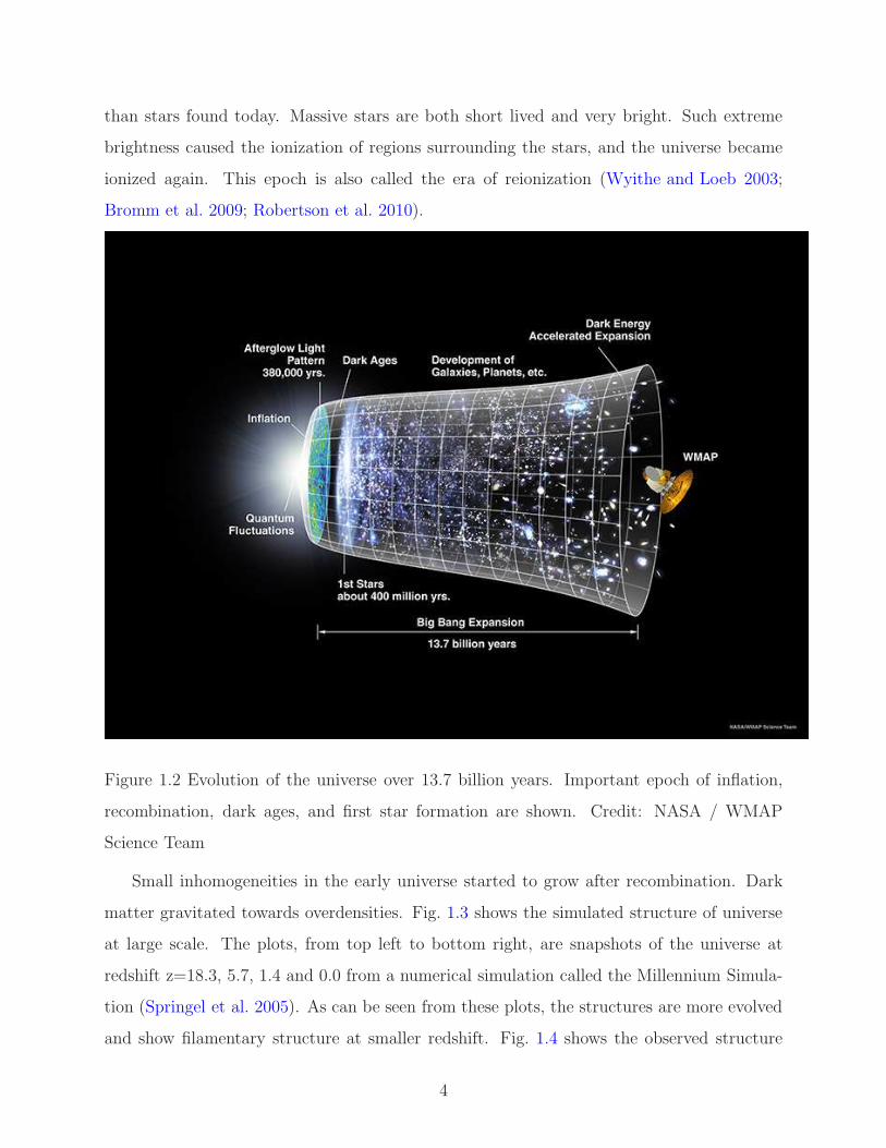
than stars found today. Massive stars are both short lived and very bright. Such extreme
brightness caused the ionization of regions surrounding the stars, and the universe became
ionized again. This epoch is also called the era of reionization (Wyithe and Loeb 2003;
Bromm et al. 2009; Robertson et al. 2010).
Figure 1.2 Evolution of the universe over 13.7 billion years. Important epoch of inflation,
recombination, dark ages, and first star formation are shown. Credit: NASA / WMAP
Science Team
Small inhomogeneities in the early universe started to grow after recombination. Dark
matter gravitated towards overdensities. Fig. 1.3 shows the simulated structure of universe
at large scale. The plots, from top left to bottom right, are snapshots of the universe at
redshift z=18.3, 5.7, 1.4 and 0.0 from a numerical simulation called the Millennium Simula-
tion (Springel et al. 2005). As can be seen from these plots, the structures are more evolved
and show filamentary structure at smaller redshift. Fig. 1.4 shows the observed structure
4

of our local universe, where each point denotes a real galaxy. The filamentary structure, as
predicted by the simulation, is evident in the observed data, leading to the conclusion that
ordinary matter follows the dark matter potential.
Figure 1.3 Computer simulation of large-scale structure of universe from the Millennium
Simulation. From top left to bottom right the structure at redshift z= 18.3, 5.7, 1.4 and
0.0 respectively. The bar in each figure shows the scale of 125 Mpc/h. (Springel et al. 2005,
http://www.mpa-garching.mpg.de/galform/virgo/millennium)
The structures continued to evolve, enhancing inhomogeneity. Baryons condensed in
these overdensities and began to form more complex object than stars (e.g., proto-galaxies,
quasars, galaxies, galaxy clusters etc.). Quasars are known to have existed as early as
redshift 7.085, which is only 0.77 billion years after the Big Bang (Mortlock et al. 2011).
Formation of baryonic structure at any time affects the formation and evolution of subsequent
structure, hence understanding the structures at all epochs is important to achieve a complete
understanding of evolution of universe.
5

Figure 1.4 Structure of the local universe. The points are location of galaxy, the filament
structures of large scale are evident from the figure. Courtesy: Michael Blanton/SDSS III
1.3 QUASARS
Quasars are extremely bright sources of light, exceeding trillions of times the brightness of
the Sun (∼ 2× 10¹²L), and yet they are point-like objects on the sky, suggesting that they
are much smaller than galaxies. A quasars’s brightness makes it observable across the visible
universe.
Quasars are believed to be powered by accretion around super massive blackholes (SMBH)
at the center of galaxies (Urry and Padovani 1995). Super massive blackholes (SMBH) are
black holes that are typically hundreds of millions of solar masses. The accretion disk around
the SMBH feeds the black hole to cause powerful jets. The accretion disk radiates due to
heat caused by gravitational potential and compression. Quasars are often a few hundred
6

times brighter than the galaxy in which they reside. Extreme radiation near quasars ion-
izes the surrounding gas. Strong winds from the quasar accretion disk blow the ionized gas
out into the environment of the quasars (Balsara and Krolik 1993; Krolik and Kriss 1995;
Proga et al. 2000; Krolik and Kriss 2001; Proga and Kallman 2004; Everett 2005).
In this thesis, I make extensive use of quasar observations to improve the understanding
of baryons in quasar systems, as well as using them as background light to understand inter-
galactic material in the universe. In the next few sections, I discuss the history and present
understanding of these fascinating objects.
1.3.1 Discovery and Basic Nature of Quasars
The discovery of quasars is a result of the development of radio astronomy. The existence
of cosmological sources of radio waves was established in the 1950’s. The polarization of
these radio waves suggested the origin to be a synchrotron processes, in which the moving
electrons radiate in the presence of a magnetic field. The estimated energy output from
these objects was so large that the idea of a gravitational potential from normal matter as
the source of energy was soon shelved. As the resolution of radio telescopes improved, the
search for the optical counterparts of these radio sources caught on. The first few identified
optical counterparts looked like stars, and their redshifts were identified from optical spectra.
These redshifts suggested that the distances to the systems were on a cosmological scale;
the redshifts/distances enabled the estimation of the energy output of these systems. These
star-like objects, being very compact objects, emitting energy that was hundreds of times
the output of a galaxy, were called Quasi-Stellar Objects (QSO) or quasars.
The early definition of a quasar was summarized by Burbidge (1967) as follows:
• star-like object identified with a radio source
• variable light
• large ultraviolet flux of radiation
• broad emission lines in the spectra with absorption line in some cases
• large redshift
7

The theoretical understanding of quasars progressed with the observations in the early
days. Hoyle and Fowler (1963) suggested that compact gravitationally collapsed objects
could serve as the energy source for such energetic objects. The existence of jets in early iden-
tified quasars also suggested the existence of violent processes (Rees 1967; Blandford and Rees
1974). These ideas soon led to the following picture of quasars: an accretion disk is formed
around a super-massive black hole, many orders of magnitude larger than the mass of typical
stars, with jets coming out perpendicular to the accretion disk. With advances in theoret-
ical understanding of in-falling material on to a compact object (e.g., neutron star, black
hole), the understanding of accretion disks a torus-like thick disk in the quasar environment
was established (Shakura and Sunyaev 1973; Lynden-Bell and Pringle 1974). Even though
a detailed understanding of quasars is still elusive, the existence of an accretion disk and a
thick torus around a super-massive blackhole (SMBH) with jets coming out from the pole is
still accepted as the current basic description of quasars.
1.3.2 Unified Quasar structure
Since the discovery of cosmological radio sources and their optical identification, there have
been many observational efforts undertaken to try to identify these non- typical objects, using
various ranges in the electro-magnetic spectrum, from radio to X-ray. Various classifications
of objects that are not typical stars or galaxies have come from these efforts. The objects
are classified in various categories according to the properties of their spectra. Below I give
a brief description of a select few.
Seyfert Galaxies: First identified by Seyfert (1943), these galaxies contain bright star-
like nuclei and their spectra have broad emission lines. With identification of more such
galaxies, Seyfert galaxies were further classified as type 1 and 2. The type 1 Seyfert galaxy
nucleus has a strong continuum from far infrared to X-ray. The few emission lines are
generally broad but some narrow emission lines can be present. The type 2 galaxy nucleus
has a much weaker continuum and only contains narrow emission lines.
Radio Galaxies: Radio galaxies are galaxies which are identified as radio sources.
Most of these galaxies have an elliptical morphology. The radio emission shows a complex
8

morphology for the radio emitting region. Radio galaxies are further classified according
to emission line properties as Broad-Line Radio Galaxy (BLRG) and Narrow-Line Radio
Galaxies (NLRG). As the name suggests BLRGs have some emission lines which are broad,
while in NLRGs, all the emission lines are narrow.
Blazars: This family of objects shows rapid variability and features a spectrum domi-
nated by non-thermal emission. Blazars are subdivided into BL Lac and OVV subclasses.
BL Lac objects are generally strong X-ray sources. These objects do not show strong emis-
sion lines. They also demonstrate high polarization and are a strong source of radio emission.
Optically violent variable (OVV) quasars show rapid variation in their optical spectrum.
These diverse classes of object, though having many peculiarities, have many underlying
similarities. These similarities naturally give an opportunity to attempt a unification of these
classes with a general model using only few basic parameters. While many theories that have
attempted to unify a few classes have enjoyed limited success, the attempt to unify various
classes is far from over. I present here the most popular unification scheme. The review
article Urry and Padovani (1995) covers this scheme in great detail. The level of scientific
verification varies for different parts of the model.
Quasars originate from matter falling in to a SMBH at the center of the galaxy. The
falling gas forms an accretion disk. The viscous and turbulent processes in the accretion
disk cause the gas to lose angular momentum, thus bringing it closer to the event horizon
of the black hole. During this process, the accretion disk heats up and glows brightly in
ultraviolet and soft X-rays. Hard X-rays are produced very near to the black hole emitted
by hot electrons. The rapidly moving gas cloud in the potential of the SMBH produces strong
emission lines in the optical and ultraviolet. There is a thick torus made of gas and dust
aligned with the accretion disk. The torus obscures the SMBH and the associated broad-line
emission gas cloud from lines of sight near the equatorial plane. Gas clouds away from the
torus produce narrow emission lines. The SMBH also forms jets of energetic particles in the
direction of the poles. These jets interact with the Inter-Stellar Medium (ISM) and produce
radio emission. Thus in an elliptical galaxy, due to more ISM in the direction of jets, the
radio sources are strong compared to the spirals. The lines of sight near the equatorial
plane are blocked by the dusty torus, preventing observation of the broad emission line gas
9

cloud, resulting in spectra with only narrow emission lines. The above picture of the SMBH
region in galaxies attempts to explain the different classes of observed spectra as differences
in viewing angle, mass and spin of the SMBH, and accretion rate. Details of these processes
are still not resolved.
One of the important features of the unified scheme is the outflow of the gas from the
accretion disk. The origin of such outflows is not very well understood. The outflow may
be accelerated by magneto-centrifugal forces, or by radiation pressure, or by pressure driven
wind, depending on the different model. In the case of an outflow dominated by radia-
tion pressure, the flow is confined to low latitudes with respect to the accretion disk plane.
According to simulations (Proga et al. 2000; Proga and Kallman 2004), some transient fil-
aments of higher density form. In the case of outflows dominated by magneto-centrifugal
forces, the flow is more cylindrical (Everett 2005). In the case of outflows dominated by
gas pressure, the wind is generated from the cool, dense torus, by photo-evaporation; there-
fore the wind does not originate deep inside the potential well, and it has a smaller outflow
velocity (Balsara and Krolik 1993; Krolik and Kriss 1995, 2001).
1.3.3 Quasar Properties
The quasar spectrum shows broad emission lines in the ultraviolet and optical parts of the
spectrum. At high redshift, the most commonly observed emission line is C IV, due to
redshifting of ultraviolet features into the observable optical range. These emission lines
are generated very near to the accretion disk of SMBH and an intrinsic part of quasars.
Baldwin (1977) was the first to observe the anti-correlation between luminosity and the
equivalent width of C IV. The effect has been confirmed by many studies (e.g., Wu et al.
2009; Richards et al. 2011) and is due to a lack of atoms in higher ionizing states, because
of the lack of ionizing photons in low brightness quasars.
Quasars emit over a very broad range of the electro-magnetic spectrum and are bright
in ultraviolet through X-ray. They exhibit an anti-correlation of ultraviolet luminosity and
X-ray luminosity. More specifically, there is a suggested nonlinear inverse scaling of 2 keV
X-ray luminosity with the ultraviolet luminosity at 2500 A (Avni and Tananbaum 1982;
10

Green et al. 1995; Steffen et al. 2006; Just et al. 2007; Richards et al. 2011)
It is also well observed that the emission lines in quasar spectrum are systematically
blue-shifted compared to the true redshift. The blue-shift varies for different emission lines,
with a more severe blue-shift for higher ionization lines. The blue-shift also depends on
the luminosity, though the luminosity dependence is much weaker in radio-loud quasars
compared to radio-quiet quasars (Richards et al. 2011).
1.3.4 Significance of Quasars for cosmology
Quasars are a very useful probe for enhancing our understanding of cosmology. The quasars
observed at redshift ∼6 provide a wealth of information about the epoch of reionization
(Becker et al. 2001; Fan et al. 2001, 2003; White et al. 2003; Djorgovski et al. 2006). They
are one of the very few tools available to us to probe this epoch.
Quasars could have a significant effect on the evolution of baryonic objects (e.g., galax-
ies). The highly energetic narrow jets and less energetic but broader outflows give a sig-
nificant amount of energy to the surrounding ISM. Such a feedback process has been hy-
pothesized to regulate the evolution of the galaxies (Silk and Rees 1998; Springel et al. 2005;
Di Matteo et al. 2005; Bower et al. 2006).
Quasars are also very useful in probing everything along their sight-line. The intervening
objects between the quasar and us often imprint absorption features in spectra. These
absorption lines (QALs) provide information about the quasar environment as well as the
Inter-Galactic Medium (IGM). QALs have been used to study a broad range of subjects,
ranging from quasar environments (e.g., Foltz et al. 1988; Aldcroft et al. 1994; Richards 2001;
Ganguly et al. 2001; Baker et al. 2002; Vestergaard 2003; Yuan and Wills 2003; Richards
2006; Ganguly et al. 2007; Lundgren et al. 2007; Misawa et al. 2007; Ganguly et al. 2007)
to large scale clustering (for example,Petitjean and Bergeron (1990); Steidel and Sargent
(1992); Petitjean and Bergeron (1994); Outram et al. (2001); Churchill et al. (2003)
Adelberger et al. (2005); Bouche et al. (2006); Scannapieco et al. (2006); Wild et al. (2008);
Tytler et al. (2009) Lundgren et al. (2009); Crighton et al. (2011))
11

1.3.5 Understanding the origin of quasar absorption systems
The star formation rate peaked between redshift '2 and '3 and decreased by an order of
magnitude by the present day (Hopkins and Beacom 2006). Since stars are the only source
for elements heavier than lithium, the QALs at this redshift range are a great tracer of star
formation and galaxy evolution. One of the most easily detectable absorber systems at this
redshift is triply ionized carbon (C IV). The C IV transition at wavelength 1549A is in the
ultraviolet range (100-4000A) of the spectrum, but since the photons are redshifted, they
reach us in the optical part of the spectrum, if they originate at a redshift greater than 1.5.
We can understand the origin of these C IV systems by measuring their clustering strength.
For example, in the simple model where C IV systems originate from population III stars,
C IV systems would be more homogeneously distributed and their clustering strength would
be similar to the strength of the dark matter itself. However, if the C IV gas originated
in star-forming galaxies and was expelled by supernova blast waves into the intergalactic
medium, we would expect the C IV systems to have a higher clustering strength matching
that of star-forming galaxies. Alternatively, if the C IV systems result from quasars and are
expelled by outflows, we would expect the C IV systems to have a strong clustering strength
similar to quasars. Our understanding of structure formation by dark matter enables us to
use the clustering strength of dark matter halos to find the mass of the halo at any epoch.
Since C IV (like any baryon) traces the dark matter, the clustering strength measurement
gives the mass of the host halos of these systems.
Measuring clustering strength requires an accurate understanding of observational con-
straints and the selection effects due to these constraints. The complexity of constraints of
quasar observations along with extracting the absorber’s information from the spectra makes
it difficult to directly measure the clustering strength of C IV. However, ever-useful quasars
help us determine the clustering strength indirectly by measuring the clustering strength
of C IV with respect to a quasar. We have numerous observations of quasars in the same
volume as the CIV absorbers, and the understanding of their population is quite accurate. In
Chapter 2, I determine the clustering strength of C IV absorbers by measuring their relative
clustering with quasars.
12

1.3.6 Understanding Quasars using absorption lines
Many quasar spectra demonstrate various QALs, (e.g., Mg II, C IV, Ly-α, Ly-β, Si IV,
Fe II). These are generally subdivided as Broad Absorption Line (BAL) or Narrow Ab-
sorption Line (NAL). These absorption features are an excellent way to probe the environ-
ment of the quasar, as some physically reside in this environment (Weymann et al. 1979;
Yuan and Wills 2003; Richards 2006; Ganguly et al. 2007; Lundgren et al. 2007; Foltz et al.
1988; Aldcroft et al. 1994; Ganguly et al. 2001; Baker et al. 2002; Vestergaard 2003; Richards
2001; Misawa et al. 2007; Ganguly et al. 2007). C IV gas clouds are frequently observed in
the quasar spectrum with redshift similar to that of the quasar, making them the obvious
candidate to probe the quasar environment. In Chapter 3 we study the quasar environment
using the C IV absorbers associated with quasars. However, all C IV clouds observed in the
quasar spectrum are not due to their local environment. The intervening space also makes a
significant contribution, but because we only observe velocity not actual distance, it is hard
to classify them according to their origin. We can improve our study if we try to account for
C IV clouds statistically rather than individually. In Chapter 3, we estimate the intervening
component and use it to estimate the population and properties of C IV clouds in quasar
environments.
At redshift '1, the dark energy started to have non-negligible influence on the rate of
expansion of the universe. By redshift '0.3 the dark energy became the dominant component
of energy density and improving our understanding of dark energy has assumed foremost
importance in understanding our present-day universe.
1.4 SUPERNOVA
Supernova Ia cosmology burst onto the center stage of cosmology by discovering acceleration
of the expansion of universe (Riess et al. 1998; Perlmutter et al. 1999). The acceleration is
attributed to a component of the universe that has a negative pressure, which is called Dark
Energy. The negative pressure leads to the acceleration of expansion of the universe, as
13
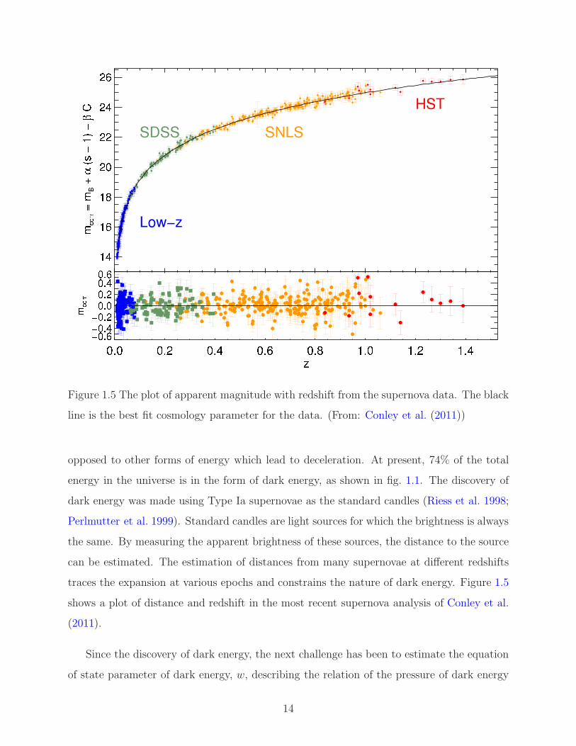
Figure 1.5 The plot of apparent magnitude with redshift from the supernova data. The black
line is the best fit cosmology parameter for the data. (From: Conley et al. (2011))
opposed to other forms of energy which lead to deceleration. At present, 74% of the total
energy in the universe is in the form of dark energy, as shown in fig. 1.1. The discovery of
dark energy was made using Type Ia supernovae as the standard candles (Riess et al. 1998;
Perlmutter et al. 1999). Standard candles are light sources for which the brightness is always
the same. By measuring the apparent brightness of these sources, the distance to the source
can be estimated. The estimation of distances from many supernovae at different redshifts
traces the expansion at various epochs and constrains the nature of dark energy. Figure 1.5
shows a plot of distance and redshift in the most recent supernova analysis of Conley et al.
(2011).
Since the discovery of dark energy, the next challenge has been to estimate the equation
of state parameter of dark energy, w, describing the relation of the pressure of dark energy
14

to the energy density of dark energy. The next generation of surveys, such as ESSENCE
(Miknaitis et al. 2007), aimed to measure the w of dark energy. Due to the increased number
of observed supernovae, the statistical uncertainty in supernova analysis has decreased. How-
ever, there remain many systematic uncertainties due to various assumptions and unknowns.
The systematic uncertainties of supernova analyses now exceed the statistical uncertainties.
It is now imperative to understand the systematic uncertainties so that further progress can
be made.
In Chapter 4, I estimate w and the systematic uncertainty carefully for the ESSENCE
supernova survey. In next few sections, I describe the history and current understanding of
supernova Ia, which have changed our understanding of the universe in a very significant
way in the last decade.
1.4.1 Supernovae Ia and Properties
Supernovae are a transient event following the explosion of a star. At their peak brightness,
they can match the brightness of the galaxy in which they reside. Since they are very bright,
supernovae can be seen to large distances and probe the universe in the distant past. Their
standard brightness can be used as a tool to measure their distances. They are also factories
for making and distributing new elements, making them important for galaxy evolution and
composition in the universe.
Supernovae have been centers of curiosity since the 20th century. In early observations,
they were described as “novae” (new stars). In a famous debate between Shapley and Curtis,
they argued about the nature of these “novae”. Shapley (1921) argued them to be novae
and thus nearby objects. Curtis (1921) argued them to be in separate galaxies and to be
inherently different objects compared to novae. The debate has been detailed in Trimble
(1995). Using the locally observed properties of Cepheid variables-the period of oscillation
in luminosity correlates with luminosity-Hubble deduced the distance of nearby galaxies
(Hubble 1925). Hubble’s famous plot of distance vs redshift of nearby galaxies established
the view of the expanding universe; such plots are now are called “Hubble diagrams”. This
firmly established the extra galactic origin of these “novae”, resolving the debate.
15

Baade and Zwicky (1934) were the first to use the name “supernovae” for these extra
bright “novae”, and were also the first to try to explain supernovae physically, by speculating
that they are collapsing neutron stars. Baade (1938) was the first to highlight the uniformity
of brightness in the supernova data, which made them appropriate to be used as “standard
candles”. The need for classification arose when Minkowski (1941) found a spectrum of a
supernova that was very different than previously observed. The supernovae from Baade
(1938) had not shown any hydrogen in their spectra. They were called Type I supernovae
(SN I), while the new supernova was classified as Type II. The first attempt to make a
Hubble diagram using 19 supernovae was made by Kowal (1968).
Pskovskii (1968) noticed the presence of broad and deep absorption observed at about
6150A, due to Si II at the maximum brightness, in many SN I. Supernova classification
evolved with better spectra and further understanding of noise. Supernovae Type Ia (SN Ia)
are currently described as supernovae which do not show any sign of Hydrogen or Helium
but show a distinctive SiII absorption feature at peak brightness. SNe Ia are now understood
to be thermo-nuclear reactions during which the white dwarf is totally disintegrated by the
energy. All other supernovae are core-collapse, where the central region of an evolved star
is converted to a neutron star or black hole due to pressure, and the outer layers are blown
away due to shock.
With the advent of CCDs and more accurate measurement of light from SN Ia, it became
clear that SN Ia had substantial variation in luminosity. The brighter SNIa’s are about three
times brighter than the dimmer ones. Phillips (1993) demonstrated the correlation between
the luminosity and the rate of rise and fall of luminosity (light curve) of the SN Ia, also
referred to the as brighter-slower relationship: brighter SN Ia rise and fall in luminosity
slower. It was observed for SNe Ia that the higher the luminosity, the shallower the slope
of the light curve tends to be. The correction for this correlation significantly reduced the
scatter of SN Ia on the Hubble plot. Figure 1.6 shows the effect of the correction of this
correlation. The discovery pointed to a need to find more very well observed SN Ia at
various epoch, in the local universe, so that more properties could be found to improve the
standardness of SN Ia as standard candles.
Along with improvements in making SN Ia better standard candles, there were attempts
16

to verify the distance estimation of SN Ia independently. Sandage et al. (1992); Saha et al.
(1995) used HST images to identify Cepheid variables in type Ia host galaxies. These studies
established the supernova Ia absolute magnitude at MV = −19.52 ± 0.07 mag and MB =
−19.48 ± 0.07 mag.
Because SN Ia suffer from extinction due to dust, the distance measurement is difficult.
A significant improvement in measuring dust extinction was achieved when Lira (1995)
first noticed that all SN Ia reach a common color after 30-90 days of maximum brightness,
irrespective of their luminosity. Due to improvement in the dust extinction measurement,
allowing a more precise measurement of the color of supernova, Riess et al. (1996) noticed
the color of SN Ia correlates to luminosity, which is often referred to as the “brighter-bluer”
relation where the brighter SN Ia tend to be bluer in color.
Significant improvement in the technology of making telescopes and computational power
led to further improvement. Riess et al. (1998) and Perlmutter et al. (1999) made the break-
through discovery about the accelerating universe using SN Ia as standard candles, a dis-
covery that made SNe Ia central to modern cosmology.
1.4.2 Progenitors of Supernova Ia
Improved knowledge of the SN Ia progenitor would be immensely useful for SN Ia cosmology.
Understanding the progenitor systems could lead to significant improvement in understand-
ing the evolution of various systematics with redshift and possibly their correlation with each
other. It could also give guidance to suggestions of physical parameters which might make
SNe Ia better standard candles. Even though the importance of SN Ia to cosmology can not
be overstated, the basic understanding of its progenitor still eludes us.
SN Ia’s are thought to be thermo-nuclear explosions of a carbon-oxygen white dwarf,
which are at, or close to, the Chandrasekhar limit of 1.4 M (Hoyle and Fowler 1960).
One widely accepted progenitor is a carbon-oxygen white dwarf that grows in mass
through accretion from a non-degenrate stellar companion (i.e., main sequence star, subgaint
star, helium star, red giant star; Whelan and Iben 1973). The accreted matter increases the
pressure in the white dwarf above the limit that can be supported by the degeneracy pressure
17

Figure 1.6 Top panel shows the different SN Ia light curves. The vertical axis is brightness and
horizontal axis is time in the rest frame of SN Ia, in reference to time of maximum brightness.
The bottom panel show the same light curves, taking into account the correlation between
brightness and shape. This figure demonstrates that the scatter in luminosity of SN Ia is
reduced significantly once the correlation is taken into account (Coursey: Kim et al. 1997).
18

of electrons. At this point, the nuclear burning starts and within seconds completely destroys
the star. A large fraction of the star burns completely to Ni56. The radioactive decay of Ni56
powers the light curve that we observe (Colgate and McKee 1969). Figure 1.7 (a & b)shows
a cartoon picture of this progenitor model, which is also known as Single Degenerate.
Another model of the progenitor involves two white dwarfs merging after losing energy
and angular momentum to gravitational waves (Figure 1.7 (c)). Such a merger may lead
to an object more massive than the Chandrasekhar limit, which can ignite and explode.
Alternatively, the process of merging might disintegrate the smaller white dwarf and may
lead a super-Chandrasekhar limit white dwarf (Iben and Tutukov 1984; Webbink 1984).
Since these models involve two degenerate objects, they are called Double Degenerate.
Both of the models were suggested many decades ago but even today there is no clear
preference for any model. There is, in fact, much observational evidence against each model
(e.g., Maoz and Mannucci 2011, and references therein). The observed rate of SN Ia is an ex-
ample. The current SN Ia rate is considered, by some, bimodal, with one prompt component
which is proportional to star formation rate and a delayed component which is proportional
to total stellar mass of the galaxy (Mannucci et al. 2005; Scannapieco and Bildsten 2005).
The single degenerate model fails to explain the existence of the delayed component, but
the double degenerate model does not explain the prompt component well. Both models
under-predict the observed SN Ia rate. Both models can only explain the SN Ia in a narrow
range of some physical parameters of the model.
It is also possible that both systems result in SN Ia. The possible consequence of multi-
ple channels of progenitor is more diversity in the supernova brightness, which would reduce
their standardness. As we can see in the double degenerate case, the combined mass after
a merger can exceed the Chandrasekhar mass limit, making these supernovae brighter than
others. The multiple channel also brings a complicated redshift dependence to the super-
nova brightness. We know that in the early universe the star formation rate was much higher
than it is currently. This asymmetry in star formation rate could make the supernovae at
higher redshift systematically more fainter than the local ones, as they would have a higher
proportion of single degenerate progenitors. To make the dependence more complicated, the
brightness of supernovae is also believed to dependent on the metalicity of the progenitor in
19
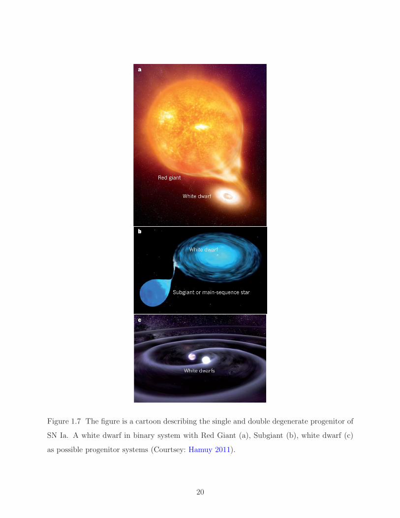
Figure 1.7 The figure is a cartoon describing the single and double degenerate progenitor of
SN Ia. A white dwarf in binary system with Red Giant (a), Subgiant (b), white dwarf (c)
as possible progenitor systems (Courtsey: Hamuy 2011).
20
the single degenerate case. Lower metalicity may make supernovae less bright (Timmes et al.
2003; Sullivan et al. 2010; Konishi et al. 2011). At higher redshift the metalicities are lower,
and because of this, these supernovae would be fainter than more recent ones. The super-
novae from double degenerate systems have a large delay time and are thus less affected by
metalicity variations as a population. As we can see, our lack of knowledge of a progenitor
limits our ability to use the SNe Ia as standard candles.
Even though the mystery of a SN Ia progenitor is far from being solved, the empirical
standaredness can still be used to provide estimates on the cosmological parameters.
21
2.0 C IV ABSORBER-QUASAR CROSS CORRELATION
The Work presented in this chapter was submitted to the Astrophysical Journal in May
2012. In this chapter, I study the clustering of C IV absorbers with respect to quasars. Such
clustering estimates can shed light on many important questions (i.e., the origin of absorbers,
feedback processes in galaxies and star formation). In §2.1, I explain the basics of absorption
system detection and their properties. The estimation of clustering is contingent upon our
understanding of large scale clustering of dark matter. In §2.2, I give a short background of
large scale clustering theory. I explain the importance and advantages of my measurement
in §2.3 in the context of cosmology, as well as the astrophysics of the host galaxies of the
C IV absorbers. In § 2.4, I explain the source of data for absorbers, quasars, and the random
comparison catalog. I explore different correlation function estimators in §2.5 and justify
my choice of the correlation estimator. In §2.6, I present the main results of this study and
compare them to previous studies. In §2.7, I estimate the contribution of various systematic
errors that could affect this result. In the last section of this chapter, §2.8, I summarize the
main findings of my study and suggest future studies that could improve my result.
2.1 ABSORPTION SYSTEMS
Quasars are highly luminous objects that are believed to be super-massive black holes (Salpeter
1964; Lynden-Bell 1969) accreting material. Being very luminous, they can be seen at large
distances; therefore, they are ideal for the study of large scale clustering at early cosmic
times. Quasars are also very useful for probing the space along the lines of sight to the
quasar. Intervening material imprints various absorption at different redshifts in the spec-
22

trum of a single quasar. Quasar absorption lines are currently thought to be from two
sources: (1) intrinsic gas in the host galaxy of the quasar and (2) intervening gas in the
galaxy along the line of sight to the quasar (e.g., Lynds 1971; Bergeron 1986; Sargent et al.
1988; Steidel and Sargent 1992; Steidel et al. 1994; Petitjean et al. 1994).
Figure 2.1 A cartoon picture of the quasar intrinsic spectrum is shown as the red line. The
green line is the spectrum we observe, which has flux absorbed by material in between us
and the quasar. The absorption lines identify the redshift and element causing absorption
from the spectrum. Courtesy: John Webb
We describe the absorption feature in the spectrum using a measure known as “equivalent
width”. The equivalent width is defined as the area enclosed by the absorption feature after
normalizing the spectrum by the continuum. Fig. 2.2 illustrates the definition of equivalent
width. The absorption profile at the left has the same area as the shaded region of width b
at the right. The value of b is the equivalent width of the absorption profile. The equivalent
width is widely used in the study of QALs, as it is a better indicator of the physical properties
of the originating system than other spectral features, such as depth.
C IV is a commonly observed QAL system in quasars. The rest-frame wavelength of the
23

UV CIV doublet transition is (1548A, 1550A), which makes it easily observable in the optical
region at redshift z > 1.5. The C IV transition being a doublet makes the identification of
such systems more robust.
Figure 2.2 Illustration of the definition of equivalent width. The shaded areas are equal in
size. The value of b is the equivalent width measurement for the absorption feature shown
on the left side. Courtesy: COSMOS - The SAO Encyclopedia of Astronomy
2.2 LARGE SCALE CLUSTERING
The theory of large scale clustering is developed assuming a smooth distribution of matter in
the early universe and small perturbations on top of that. In the limit of small perturbations,
the growth of structures can be calculated. The equations are usually written in terms of
the overdensity, δ, which is defined as
δ(~x) =ρ(~x) − ρ
ρ(2.1)
where ρ is average density of the universe and ρ(~x) is the density of the universe at location
~x. In Fourier space, different modes of overdensity evolve independently of each other. The
overdensity in Fourier space can be written as
δ(k, t) =D(t)
D(t′)T (k, t, t′)δ(k, t′) (2.2)
24

where D(t) is the growth function (Lacey and Cole 1993; Carroll et al. 1992; Bildhauer et al.
1992), which is independent of scale, and t and t′ are different epochs. T (k, t, t′) is called
the transfer function (Eisenstein and Hu 1999) and governs the evolution of overdensity of
different modes. The power spectrum, which is defined as the square of the amplitude (thus
the power) of a given mode, can be expressed as follows.
P (k) ≡ 〈|δ(k)|2〉 (2.3)
In terms of the power spectrum, the evolution of structure can be written as
P (k, t) =
(
D(t)
D(t′)
)2
T 2(k)P (k, t′). (2.4)
This enables us to calculate the power spectrum at any epoch, if we know the power
spectrum at any earlier epoch. The power spectrum at early epochs is well observed by
studying the CMB when the overdensities were small. Using the growth function and the
transfer function, we can estimate the power spectrum at any epoch quite precisely. This
power spectrum is often called the linear power spectrum as it holds in the approximation
of small overdensities where the original equation governing the evolution becomes a linear
differential equation. This power spectrum holds for dark matter, as dark matter interacts
only through gravitation and is, therefore, easier to calculate. Since the dark matter density
is much higher than the baryon density, the baryons follow the dark matter potential. At
small real distances the overdensity is not proportionally small, but averaged over large
distances, the overdensity is still extremely small and the above formalism works very well.
The overdensity of condensed baryons, like galaxies and quasars, are also small at large
scales, so it can be written for any species, x, as (Efstathiou et al. 1988; Cole and Kaiser
1989; Mo and White 1996; Sheth and Tormen 1999)
δx = bxδdm (2.5)
where bx is the bias of x. Now the power spectrum of two species x and y can be written as
Px−y(k, z) = bxbyPlin(k, z). (2.6)
25

Since all our measurements are in real space, the above equation can be rewritten in real
space by using the inverse transformation as defined below.
ξ(r, z) =1
2π2
∫
k3P (k, z)sin(kr)
krd ln k (2.7)
The cross correlation of species x and y can then be written as below.
ξx−y(k, z) = bxbyξdm (2.8)
Since ξdm can be calculated using basic physics, any observation of the cross-correlation of
species x and y leads to the determination of bxby.
2.3 MOTIVATION
The origin of intergalactic QALs is not well understood. The metal lines provide infor-
mation about the structure formation process. They could be produced, for example, by
(1) isolated initial generation of stars (population III); (2) gas ejected into the inter-galactic
medium from proto-galaxies in merger processes (Gnedin 1998); (3) gas ejected from star-
forming processes within galaxies transported to large distances by galactic superwinds
(Voit 1996; Heckman et al. 2000; Pettini et al. 2001, 2002) or jets from active galactic nuclei
(AGN) (Bahcall and Spitzer 1969; Mo and Miralda-Escude 1996; Maller and Bullock 2004;
Chelouche et al. 2008); (4) processes in the cold gas in dark matter halos (Bahcall and Spitzer
1969; Mo and Miralda-Escude 1996; Maller and Bullock 2004; Chelouche et al. 2008) around
star-forming galaxies–the subsequent growth of large-scale structure would then make their
distribution more cuspy.
One way to differentiate between these various scenarios of metal-enrichment of the inter-
galactic medium is to measure the clustering strength of the QAL systems (Adelberger et al.
2005). For example, in the simple model where QAL systems originate from population III
stars, QAL systems would be more homogeneously distributed and their correlation function
would be similar to the correlation function of the dark matter itself. However, if the QAL
gas originated in star-forming galaxies and was expelled by supernova blast waves into the
26

intergalactic medium, we would expect the QALs to have a more biased correlation function
matching that of star-forming galaxies. Equivalently, we would expect the QAL systems to
reside in the same dark matter halos in which the star-forming galaxies reside. Alternatively,
if the QAL systems are from quasars and expelled by outflows, we would expect the QALs
to have a strongly biased correlation function similar to quasars. In other words, the QALs
would reside in the same dark matter halos as quasars. The measurement of the QAL corre-
lation function thus enables us to relate the QAL systems to the mass of the halos in which
they reside.
The correlation strength of intervening QALs can also be used to better estimate the
fraction of QALs that are due to the quasar environment, and do not follow the clustering
properties exhibited by other QALs. In this document, we refer to all such QALs as “intrin-
sic,” making no distinction between systems that are sometimes more specifically referred to
as “intrinsic” or “associated.” Our definition of “intrinsic” QALs thus includes those with
high outward velocity with respect to quasars that overlap in redshift space with the inter-
galactic QALs. Understanding the correlation of the intergalactic QALs will allow for more
accurate measurements of the spatial and velocity distribution of the intrinsic QALs in the
future, and in turn, will help constrain the astrophysics of quasars and their host galaxies.
There have been many of investigations of the clustering properties of various QALs. Be-
cause most spectra are taken in optical observer-frame wavelengths, different species of QALs
have usually been studied in different redshift ranges according to their rest-frame wavelength
and uniqueness of identification. Mg II (λ =2796A,2803A) and C IV (λ =1548A,1550A)
are the two most-studied species because their prominent absorption double lines make
them easy to identify. Previous works have studied Mg II systems in a redshift range of
0.2 < z < 2 (Petitjean and Bergeron 1990; Steidel and Sargent 1992; Churchill et al. 2003;
Bouche et al. 2006; Lundgren et al. 2009). With C IV QALs we can reach the higher redshift
range of 1.5 < z < 4.
A number of efforts have been made to determine the C IV clustering strength, us-
ing various methods (Petitjean and Bergeron 1994; Outram et al. 2001; Adelberger et al.
2005; Scannapieco et al. 2006; Wild et al. 2008; Tytler et al. 2009; Crighton et al. 2011). A
few studies have measured the auto-correlation function for C IV and other absorbers (e.g.,
27
Scannapieco et al. 2006). The cross-correlation of CIV absorbers with quasars or galaxies has
been explored by (Outram et al. 2001; Wild et al. 2008; Tytler et al. 2009; Crighton et al.
2011). Adelberger et al. (2005) found that the cross-correlation function for C IV absorp-
tion systems and galaxies, based on ∼1000 absorbers, is similar to the correlation function
of star-forming galaxies. All of these studies, however, are based upon a small number of
quasars and C IV absorbers and lack the power to statistically probe the overall structure
of a large volume of the Universe. Therefore, they only constrain clustering strength with
relatively low precision.
New surveys with more uniform, accurate, and extensive data currently allow for a more
precise QAL clustering analysis. The SDSS-III Baryonic Oscillation Spectroscopic Survey
(BOSS Eisenstein et al. 2011a) provides an excellent data set for such analysis. Data Release
9 (DR9) contains high-quality spectra of ∼61,000 quasars at z > 2.1 (Paris 2012); this data
set provides almost an order-of-magnitude increase in the number of QALs over previous
C IV studies.
The ideal way to measure the clustering of C IV absorbers would be to perform an auto-
correlation study of C IV absorbers. However, determining the uniformity and completeness
of the back-lighting quasar sample together with the line-of-sight completeness of detecting
C IV absorbers in quasar spectra is a significantly challenging project that requires future
work. The BOSS quasar sample specifically targets quasars in the redshift range of z > 2.2
(Ross et al. 2012); thus there is a good overlap between the space of C IV absorbers (1.5 <
z < 4) and the target redshift range of the BOSS quasar sample.
In this chapter, I calculate the two-point cross-correlation between the BOSS C IV ab-
sorbers and the BOSS quasars, which have a well-understood selection function (White et al.
2012), to provide a better estimate of clustering of the C IV absorbers. Because both our
sample C IV absorbers and quasars are from spectroscopic data, the redshifts of each sample
are known quite accurately. Therefore, here I undertake a 3-D correlation study to extract
the most information from our data set.
Throughout this work, I assume a flat ΛCDM cosmology of ΩΛ=0.74, ΩM=0.26, w = −1,
and h = 0.72.
28

2.4 DATA
2.4.1 BOSS
BOSS is an ongoing survey with the goal of determining the expansion history of the
Universe by measuring the baryon acoustic oscillation feature using luminous galaxies at
z ∼ 0.7 and the Lyman-α forest traced by quasars (Cole et al. 2005; Eisenstein et al. 2005;
McDonald et al. 2006; Eisenstein et al. 2011a). The survey plans to obtain spectra for 1.5
million massive galaxies in order to measure the distance-redshift relation dA(z) and the
Hubble parameter H(z) with percent-level precision out to z = 0.7, using techniques that
led to the first detection of the BAO feature (Cole et al. 2005; Eisenstein et al. 2005); the
first BOSS results are given in Mehta et al. (2012); Padmanabhan et al. (2012); Xu et al.
(2012). BOSS is also extending a new method of BAO measurement using the Lyman-α
forest of 150,000 distant quasars at z ' 2.5 (McDonald et al. 2006; Slosar et al. 2011).
BOSS is a spectroscopic survey undertaken within the SDSS-III program (Eisenstein et al.
2011b). SDSS-III uses a dedicated 2.5-m telescope located at the Apache Point Observatory
in New Mexico at an elevation of 2788 m (Gunn et al. 1998, 2006). In this work, I am using
data that will be part of the SDSS Data Release (DR9), which will include all the observa-
tions taken by the BOSS prior to the summer shutdown in July 2011 and is released in July
of 2012.
2.4.2 Quasars
BOSS targets galaxies for its main BAO survey and quasars for studies of the Lyman-α forest.
Maximizing the number of quasar sight-lines, regardless of how the quasars are selected, is
the best way to detect the baryon acoustic feature in the Lyman-α forest, which is a goal of
BOSS.
It was recognized early on in the survey, however, that additional science can be done
with a homogeneous quasar sample, such as, determinations of the quasar luminosity func-
tion, active black hole mass function, and auto-correlation function. Thus, to maximize the
scientific output of the survey, the BOSS project decided to target half of the quasar sample
29

using a uniform selection algorithm (Ross et al. 2012). This subset of the quasar data is
known as the “CORE” sample. On average, approximately 40 fibers for quasars targets
were allocated per deg2 of the BOSS survey; 20 of these fibers are used for the CORE sam-
ple and another ∼ 20 targets are from the “BONUS” sample. The BONUS sample uses
targeting algorithms that incorporate all available information, even if it is heterogeneous
on the sky, and is continually updated to maximize the number of quasars observed without
regard to uniformity of selection. After initial experimentation with different selection algo-
rithms (see, e.g., Kirkpatrick et al. 2011), the algorithm denoted “XDQSO” was finalized as
the algorithm that defines the CORE sample for the rest of the survey. The details of the
XDQSO targeting algorithm are presented in Bovy et al. (2011).
The main goal of having a separate homogeneous CORE sample is to enable statistical
studies, which require understanding of the completeness of the survey. The work described
in this chapter is one study that is possible because of this CORE sample.
The BOSS survey targeting strategy divides the sky into “chunks.” During the initial
period, the targeting algorithm was held constant within each chunk and changed between
chunks. After the chunk “boss12”, the targeting algorithm for CORE was frozen, So the
BOSS CORE sample is homogeneously selected subsequent to chunk 12, and will remain
so until the end of the survey. Ross et al. (2012) provides the details of the quasar target
selection and quasar sample. For this study, we are using all BOSS chunks except boss1,
which was Stripe 82 (Stoughton et al. 2002) commissioning data. Fig 2.3 shows the redshift
distribution of the quasars in our study.
2.4.3 Random Catalog for Quasars
The construction of random catalogs that represent the selection of BOSS CORE quasars is
detailed in White et al. (2012). Because the CORE quasar target selection was in flux for
the first-year, the CORE quasar sample is not perfectly uniform. However, as the CORE
target selection algorithm is now fixed to XDQSO, the completeness of the first year data
can be estimated retroactively. For each chunk, we take the catalog of targets XDQSO
would have generated and compare it to the objects that were actually observed. From
30

1.5 2.0 2.5 3.0 3.5 4.0z
0
2
4
6
8
10
Fract
ion o
f obje
ct (
0.0
5 b
ins)
CIV (23389)QSO (37831)
Figure 2.3 Distribution of redshift for C IV absorbers (black, solid line) and quasars (red,
dashed). All quasars are from the CORE DR9 sample. There are a total 37,831 quasars and
23,389 C IV absorbers in the sample. However, our clustering analysis only makes use of the
19,701 quasars and 6,149 absorbers of equivalent width > 0.28A in the overlapping region of
the distributions from 2.1 < z < 2.5.
31

this comparison, I calculate the completeness of each sector, where a sector is a spherical
polygon, or a collection of spherical polygons, that define a survey area observed under
the same conditions. Fortunately, there is a high coincidence of target objects between
the XDQSO targets and the actual targets observed for a given chunk. Ross et al. (2012)
presented the details and a comparison of the target selection algorithms.
To reconstruct the correlation function, I need a random sample subject to the same
survey effects as the quasar sample. I used code written by Adam Meyers to calculate com-
pleteness and generate the random sample. I generated a random sample with approximately
100 times more random points the actual number of quasars to accurately sample the com-
pleteness in redshift and position on the sky. Therefore, the random sample represents an
unclustered distribution of points following the properties of the data. The random gener-
ation, completeness mask, and redshift distribution are described in detail in White et al.
(2012).
2.4.4 C IV Absorption line identification pipeline
The C IV absorbers examined in this work were extracted using a modified version of the
automated SDSS Data Release 7 (Abazajian et al. 2009) quasar absorption line identification
pipeline described in Lundgren et al. (2009) and York and et al. (2012, in prep). The pipeline
identifies features of absorption by first subtracting a pseudo-continuum from each quasar.
In each case, the pseudo-continuum is determined using a variation of a moving mean, which
has been found to robustly fit both the quasar emission lines and the flat regions over a broad
range of quasar spectral morphologies. An algorithm is then run on the normalized spectra
to identify significant absorption lines. The line-finding algorithm determines the reduced
χ2 fit to a Gaussian profile centered on each pixel of the spectrum. Errors on the equivalent
width of each feature are measured directly from the error array of the quasar spectra output
by the BOSS pipeline, and lines with ≥3σ significance are retained for identification. The
error on the equivalent width reflects the 1σ error on the best Gaussian fit to each absorption
line, as derived from the SDSS error spectrum (photon statistics) for each object. For the
rest frame equivalent width measurements, the observed error is divided by 1 + z.
32

The pipeline then attempts to identify each of the detected absorption features by match-
ing ions of different species at the same redshift. The line identification algorithm operates
by first identifying the most easily observable doublets, C IV and Mg II. The search is done
independently for each of these doublets, so systems that only have C IV or only have Mg II
are easily found. Since absorbing gas should be physically located in the foreground of
the quasar, this search is restricted to the wavelength range corresponding to a velocity of
3000 km s−1 behind the quasar, to accommodate redshift errors in the quasar sample.
The continuum fitting algorithm fits poorly around narrow emission lines, causing it to
often produce artifacts of false absorption features. For this reason, the algorithm also omits
regions of the quasar spectrum in close proximity (20 A) to narrow emission lines. Because
of our cross-correlation analysis approach, our study is not sensitive to any underestimation
of C IV absorbers caused by narrow emission lines.
For each detected doublet, an absorption redshift is determined, and the remaining
unidentified absorption lines are examined for matches to other ions at the same redshift. I
consider all C IV absorbers that have resolved doublets detected at ≥ 4σ significance.
2.4.5 The C IV sample
I use the pipeline described in §2.4.4 to find C IV absorbers in BOSS quasar spectra. As
explained in §2.4.2, there are two samples of quasars, CORE and BONUS. However, the
absorber sample does not need to use a well defined selection of quasars. I choose C IV
absorbers in the following redshift range:
zabs < min
(√
1 − βmin
1 + βmin(1 + zQSO) − 1,
7500A
1549A− 1
)
zabs > max
(
1260A
1549A(1 + zQSO) − 1,
3800A
1549A− 1
)
(2.9)
As evident from Eq. 2.9 I choose the C IV absorbers in the quasar spectra in the observed
wavelength range of 3800–7500 A. This range is chosen to avoid the noisy region of the
spectra due to spectral contamination from sky lines and our limited ability to correct for
them. I also avoid any features in the region shortwards of 1260 A in the quasar rest-frame,
as this region is contaminated by the N V line and the Lyman-α forest. Therefore, our cut
33

avoids many potential false detections at the expense of missing some real systems. This
approach leads to a redshift range for detectable C IV absorbers of 1.453 < zabs < 3.841.
Broad Absorption Lines (BALs) in quasar spectra are known to contaminate Narrow
Absorption Lines (NALs), so all spectra with C IV BALs are removed from our analysis. The
BOSS quasar catalog relies on visual examination to determine if an object is a quasar or
not. BAL absorbers are visually identified in all cases (Paris 2012). This process leads to a
first-cut catalog of 37,441 C IV absorbers.
Our aim is to study the clustering of C IV absorbers relative to quasars. Quasars are
known to emit ionized winds at high velocity, so many absorption features in quasar spectra
will be intrinsic to the quasar itself rather than due to intervening absorbers. To remove
these intervening absorbers, I apply an additional constraint of β > 0.02 with β given by
β =v
c=
(1 + zQSO)2 − (1 + zabs)2
(1 + zQSO)2 + (1 + zabs)2, (2.10)
The quantity β is the recession velocity between absorber and quasar. The cut of β = 0.02
corresponds to v = 6000 km s−1 which removes most of the intrinsic absorbers from the
sample. Previous studies used a less conservative cut for the velocity. Ellison et al. (2002)
used 3000 km s−1 and Fox et al. (2007) used 5000 km s−1.
Figure 2.4 shows the distribution of β for our sample. The excess of C IV absorbers in
0 < β < 0.02 is due to intrinsic CIV absorbers, which I remove from our sample. Intrinsic CIV
absorbers are known to contaminate the sample at much larger velocities (vanden Berk et al.
1996; Richards et al. 1999). Such contamination may affect the estimation of the correlation
function; I estimate this effect in §2.7.4. The intrinsic absorbers may reside in the host galaxy
of the quasar, be in material ejected from the quasar, or be in the clustering environment
of the quasar. Only the material ejected by the quasar, however, can contaminate the
measurement of the correlation function. All other sources of intrinsic C IV absorbers would
still contribute to the correct correlation function. To accurately describe intrinsic absorbers,
I would have to assume a model for the velocity distribution around the quasar, but such a
study is beyond the scope of this current work. Applying the β > 0.02 cuts decreases our
C IV absorber sample to 23,339 absorbers.
34

0.00 0.05 0.10 0.15 0.200
200
400
600
800
1000
1200
1400
1600
# (
0.0
02
5 b
ins)
=0.02
N>0.02=6878
N<0.02=7735
Figure 2.4 Distribution of β of the absorbers. The excess in the range 0.0 < β < 0.02 is due
to absorbers intrinsic to the quasar. The red dashed line of β = 0.02 separates the samples
in our study. After the β cut, 23,389 absorbers remain.
35

I measure the equivalent width of the doublet as the equivalent width of the 1548A line.
Catalog absorbers with rest-frame equivalent widths, Wr, ≈ 5 A can arise as artifacts of the
pipeline (due to, for example, poorly subtracted night sky lines) or from complicated blends
of multiple doublets. All absorbers with such strong Wr > 5 A features are removed from
the sample. This limit removes only 15 absorbers from our sample, leaving 23,324 absorbers.
The likelihood of false positives is higher in the small observer-frame equivalent width
absorbers, so I apply a cut on observer-frame equivalent width of W0 > 1 A. Applying
this cut provides an automatic cut on rest-frame equivalent width of Wr > 0.28A (at our
median sample redshift of z ∼ 2.3). Figure 2.5 shows the distribution of absorbers in i-band
magnitude and Wr space. The top panel shows the distribution of Wr for absorbers from
CORE and BONUS quasars. The side panel shows the distribution of i-band magnitude for
the same absorbers. After applying this cut, I am left with 20,925 absorbers.
Cross-correlating BOSS quasars and absorbers on scales out to 100 Mpc requires the two
samples to be in the same redshift range (2.1 < z ≤ 2.5). There are very few quasars at
z < 2.1 and few absorbers at z > 2.5. This redshift range restricts our final sample to 6,149
C IV absorbers, which is almost an order-of-magnitude larger than previous C IV absorbers
correlation analysies. A summary of the effects of the different cuts is given in Table 2.1.
2.5 CORRELATION ANALYSIS
The spatial correlation function, ξ(r), describes the clustering of spatial points as a function
of distance r. Similarly, the cross-correlation function, ξA−B, describes the clustering of
two species A and B at any given separation r. The cross-correlation function between a
population of C IV absorbers and of quasars, ξQSO−CIV(r), is defined as the excess probability
of finding a C IV absorber at distance r from a quasar compared to the chance of a random
coincidence:
d P (r) = nQSOnCIV (1 + ξQSO−CIV(r)) d VQSO d VCIV (2.11)
where nCIV is the mean density of CIV absorbers, and nQSO is the mean density of quasars (Peebles
1980).
36

0 1 2 3 4 5
Wr (A)
16
17
18
19
20
21
22
i
050
100150200250300
core
bonus
50 100 1500.0
2.5
5.0
7.5
10.0
12.5
15.0
17.5
20.0
Figure 2.5 The bottom left panel of the plot shows the distribution of C IV absorber rest-
frame equivalent width, Wr(A), and the quasar i-band magnitude. The color denotes the
number density of the C IV absorbers. The color-bar at the right side of the plot shows the
color-density scale. The lack of completeness for low Wr is evident as it is systematically
more difficult to detect weaker absorbers in fainter quasars. The panel at the right shows
the distribution of i−band magnitude for absorbers from the CORE and BONUS quasar
samples. Similarly, the panel at the top shows the distribution of Wr for absorbers from the
CORE and BONUS quasar sample.
37
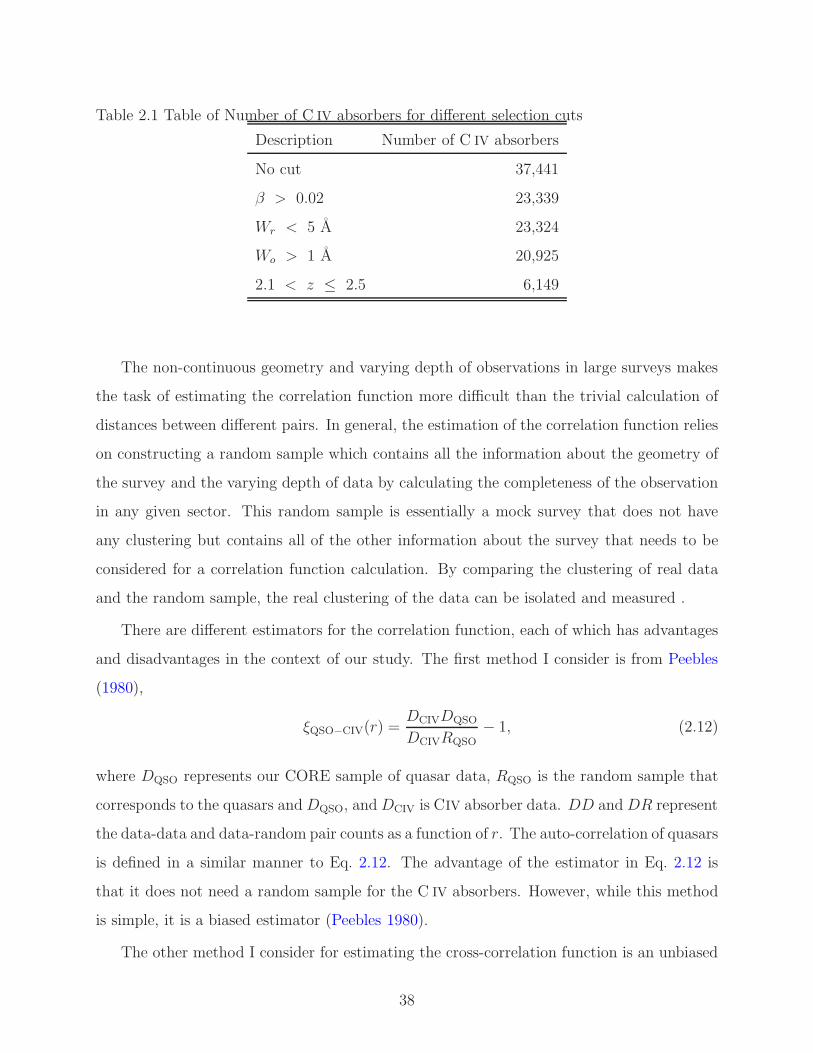
Table 2.1 Table of Number of C IV absorbers for different selection cuts
Description Number of C IV absorbers
No cut 37,441
β > 0.02 23,339
Wr < 5 A 23,324
Wo > 1 A 20,925
2.1 < z ≤ 2.5 6,149
The non-continuous geometry and varying depth of observations in large surveys makes
the task of estimating the correlation function more difficult than the trivial calculation of
distances between different pairs. In general, the estimation of the correlation function relies
on constructing a random sample which contains all the information about the geometry of
the survey and the varying depth of data by calculating the completeness of the observation
in any given sector. This random sample is essentially a mock survey that does not have
any clustering but contains all of the other information about the survey that needs to be
considered for a correlation function calculation. By comparing the clustering of real data
and the random sample, the real clustering of the data can be isolated and measured .
There are different estimators for the correlation function, each of which has advantages
and disadvantages in the context of our study. The first method I consider is from Peebles
(1980),
ξQSO−CIV(r) =DCIVDQSO
DCIVRQSO
− 1, (2.12)
where DQSO represents our CORE sample of quasar data, RQSO is the random sample that
corresponds to the quasars and DQSO, and DCIV is CIV absorber data. DD and DR represent
the data-data and data-random pair counts as a function of r. The auto-correlation of quasars
is defined in a similar manner to Eq. 2.12. The advantage of the estimator in Eq. 2.12 is
that it does not need a random sample for the C IV absorbers. However, while this method
is simple, it is a biased estimator (Peebles 1980).
The other method I consider for estimating the cross-correlation function is an unbiased
38

estimator given by Landy and Szalay (1993),
ξQSO−CIV(r) =DCIVDQSO − RCIVDQSO − DCIVRQSO + RCIVRQSO
RCIVRQSO, (2.13)
where DQSO and RQSO are the same as in the previous equation and DCIV and RCIV are the
C IV absorber sample and random sample for the C IV sample.
Eq. 2.13 is a more robust estimator, but it would require the generation of a reliable C IV
absorber random catalog. While I use Eq. 2.12 in this analysis, I would like to share some
thoughts on Eq. 2.13, as it may become the preferred method for future analyses.
The established procedure to generate randoms absorbers is to select a random point in
the sight line to the quasar in the range that absorbers could be detected. However, this
approach is not an accurate way to generate the random absorbers, as it assumes the chances
of detection and number density of the absorbers to be constant along the line-of-sight. If
the sight line covers a large enough redshift range, this assumption would affect the observed
number density of absorbers. Other effects, such as gravitational lensing, may contribute
to changes in the observed number density of the absorbers as well. I propose that future
analysis based an approach that uses Eq. 2.13 use a different two-step procedure. First, a
random quasar sample should be generated, which provides the locations on the sky. Second,
absorbers should be assigned redshifts, drawing from the observed redshift distribution of
the absorbers. This distribution may be a function of completeness of the survey. This
procedure would yield two advantages over our current use of Eq. 2.12; it would not have to
make any assumption about the evolution of number density and probability of detection,
and it will reduce the effect of survey edges on the correlation function.
However, I can not use Eq. 2.13 because I need a larger sample of absorbers to estimate
the redshift distribution for different completeness bins of quasars. At the conclusion of the
BOSS survey, it will cover a large footprint with high completeness, and we will be able to
generate a random sample that accurately follows the absorber population.
For the current study, I choose the estimator in Eq. 2.12, which does not require random
absorbers for C IV.
In addition to redshift-space three dimensional correlation fucntion, I also calculate the
projected cross-correlation function for the C IV absorbers and quasars. The redshift-space
39

distance, s, between a C IV absorber and quasar can be decomposed into components per-
pendicular (rp) and parallel (π) to the line of sight
s2 = r2p + π2. (2.14)
I can estimate the two-dimensional cross-correlation function as
ξ(rp, π) =DCIVDQSO(rp, π)
DCIVRQSO(rp, π)− 1 (2.15)
and the projected cross-correlation function is defined as
wp(rp) = 2
∫
∞
0
ξ(rp, π)dπ (2.16)
2.5.1 Error Estimation
Correlation function studies have used different methods of error estimation. These methods
can be broadly placed in three categories: Poisson, Field-to-Field, and Jackknife. The
Poisson error is simplest, but it assumes that the pair counts on different distance scales
are independent. However, the Poisson error is known to underestimate the error at large
distances, where the Poisson error is small and the cosmic variance term becomes comparable
or bigger than the Poisson error (Myers et al. 2005; Ross et al. 2007), such that the Poisson
counts are correlated across different scales. In this study, I choose to use the jackknife
method, following Scranton et al. (2002).
I partition the data into 25 different areas which have roughly the same number of quasars
from our random quasar catalog. I calculate 25 separate cross-correlation functions, leaving
out one chunk at a time. Using the 25 cross-correlation functions, I estimate the covariance
matrix from
Covij =N − 1
N
N∑
i=1
(
ξ(ri) − ξ(ri)) (
ξ(rj) − ξ(rj))
(2.17)
where N = 25 is the number of cross-correlation functions, ri and rj are the points where the
correlation function are estimated, and ξ(ri) is the correlation function for the full sample at
rj. The diagonal element of the covariance matrix Covii is the error estimate for the variance
σ2ii of the two-point correlation function in the ith bin.
40

2.5.2 Fitting for the Correlation Function and Bias
A standard way to model the two-point correlation function is using a power law given by
ξ(r) =
(
r
r0
)−γ
(2.18)
which is a good approximation for the correlation function to large distances and also a
convenient form to compare with other results. The assumption of a power-law form for the
correlation function in real space leads to a projected-space correlation function, defined in
Eq. 2.16, of the following form
wp
rp
=
(
r0
rp
)γ
B
(
1
2,γ − 1
2
)
(2.19)
where B(a, b) is the Euler beta function. In reality, I can not integrate in the line-of-sight
direction to infinity. If I choose to select the maximum line-of-sight distance, πmax, as our
integration limit, I can write
wp
rp
=
(
r0
rp
)γ [
B
(
1
2,γ − 1
2
)
− B
(
r2p
r2p + π2
max
;1
2,γ − 1
2
)]
(2.20)
where wp is the projected correlation function integrated to πmax and B(z; a, b) is the incom-
plete beta function.
To fit the correlation function in the above form, I minimize
χ2 = [ξ − ξ]T Cov−1[ξ − ξ] (2.21)
where ξ is value from the model. However, in general, the covariance matrix is too noisy to
be useful, so I only use the diagonal element of the covariance matrix.
Baryonic matter traces the gravitational potential created by dark matter and scales as
a function of the dark matter (DM) halo mass (Bardeen et al. 1986; Cole and Kaiser 1989;
Mo and White 1996; Sheth and Tormen 1999; Sheth et al. 2001; Jing 1998; Gao and White
2006; Tinker et al. 2010). The observed two-point correlation function of baryonic material
is related to the underlying dark matter two-point correlation function, as explained in §2.2.
If I assume a linear bias (Scherrer and Weinberg 1998), or baryon/DM ratio, then I can write
ξCIV−QSO(r) = bCIVbQSOξDM(r), (2.22)
41

ξQSO−QSO(r) = b2QSOξDM(r), (2.23)
similar to Eq. 2.7. I can thus find the bias for CIV absorbers without knowing the underlying
dark matter two-point correlation function. In terms of the other observable quantities
ξQSO−QSO and bQSO, the C IV absorber bias is
bCIV =ξCIV−QSO
ξQSO−QSObQSO (2.24)
The bias of a dark matter halo as a function of mass can be derived theoretically
(Bardeen et al. 1986; Cole and Kaiser 1989; Mo and White 1996; Sheth and Tormen 1999;
Sheth et al. 2001), but more accurate descriptions of halo bias can be derived from large-
scale dark matter simulations (Jing 1998; Gao and White 2006; Tinker et al. 2010). Using
such a calibration of the dark matter halo bias, I can find the mass of the dark matter halo
in which a typical C IV absorber resides.
2.6 RESULTS
Table 2.2 summarizes our measurements of the correlation length and slope for the C IV
absorber and quasar correlation functions.
2.6.1 Cross Correlation of C IV absorbers and quasars
Figure 2.6 presents our calculated three-dimensional cross-correlation of C IV absorbers and
quasars in redshift space in the redshift range of 2.1 < z < 2.5. Fitting the cross-correlation
in the range of 10 Mpc< s <100 Mpc with a power law, as described in Eq. 2.18, I find
the correlation-length to be so = 8.46 ± 1.46 Mpc with a slope γ = 1.68 ± 0.27. For the fit
I found χ2/D.o.f = 10.88/8 = 1.36, which suggests it is a quite reasonable fit to the data.
However, there is significant degeneracy between the parameters so and γ, as changes due
to an increase in slope can be caused by the increase of correlation length. The correlation
coefficient between s0 and γ for our fit is 0.86, which suggests a high degree of correlation.
42

The cross-correlation measurement is expected to be not accurate in the range of s < 10 Mpc,
because at this scale, fiber collision is expected to contaminate the astrophysical clustering
signal (Ross et al. 2009).
Figure 2.7 presents the projected cross-correlation of the C IV absorbers and quasars in
the same redshift range 2.1 < z < 2.5. I fit the cross-correlation in the range of 10 Mpc<
rp <100 Mpc with a power law, as described in Eqs. 2.19 & 2.20. I find the best fit power-
law length to be r0 = 7.76 ± 3.80 Mpc with a slope γ = 1.74 ± 0.21. I integrate the
correlation function in the line-of-sight direction until πmax = 60 Mpc and find a χ2/D.o.f =
9.20/8 = 1.15. The estimates of the length scale and power-law slope are highly degenerate
as indicated by a correlation coefficient of 0.96.
2.6.2 Cross-Correlation at large distance
Figure 2.8 shows the correlation function in the range of 10 Mpc< s <1000 Mpc in bins
of 10 Mpc. The errors are Poisson errors. The blue line is the best-fit cross-correlation
function. I find that the power-law fit does not fit the data for distances s > 100 Mpc.
This disagreement potentially expected as there is no reason the correlation function should
be well-approximated by a power-law at large distances, but this measurement provides
quantitative confirmation of the significant variation from the simple power-law model. Both
the observed and simple models for the correlation function gradually approach zero at larger
distances. Cosmic variance can contribute a small offset from zero at all scales, which is
evident only at large scales when the correlation is very close to zero.
2.6.3 Estimation of C IV bias
One of the major aims of this work is to calculate the bias of C IV absorbers with respect
to linear matter perturbations. I use a cross-correlation between the QSO sample and the
C IV sample to best estimate this bias. Ideally, one would use the C IV auto-correlation, but
the appropriate random set for the QSO sample is far better understood than for the C IV
sample. A proper generation of randoms for the absorber sample would require a model of
the evolution and distribution of C IV absorbers as a function of redshift. Providing rough
43

10 30 50 70 100
s(Mpc)
10-2
10-1
100
(s)CIV QSO 3-d cross-correlation(6149)
Figure 2.6 Cross-correlation function in redshift space for C IV absorbers and quasars from
2.1 < z < 2.5. The dotted line is the best-fit power law, as defined in Eq. 2.18, with
so = 8.46 ± 1.46 Mpc and slope γ = 1.68 ± 0.27 in the range 10 Mpc < s < 100 Mpc. The
horizontal axis denotes the geometric mean of the bin distance. The vertical error bar is the
jackknife error.
44

10 30 50 70 100
rp (Mpc)
10-2
10-1
100
wp/r p
CIV QSO projected correlation(6149)
Figure 2.7 Projected correlation function for C IV absorbers and quasars. The dotted line
is the best fit power law, as defined in Eqs. 2.19 and 2.20, with r0 = 7.76 ± 3.80 Mpc and
slope γ = 1.74 ± 0.21 in the range 10 Mpc < rp < 100 Mpc. The horizontal axis denotes
the geometric mean of projected distance bin. The redshift range for the C IV absorbers and
quasars is 2.1 < z < 2.5.
45

0 200 400 600 800 1000
s Mpc
0.0
0.1
0.2
0.3
0.4
(s)
Figure 2.8 Correlation function for 10 Mpc< s < 1000 Mpc with a bin size of 10 Mpc.
The errors are calculated using Poisson re-sampling. The redshift range for the data is
2.1 < z < 2.5. The blue dash-dot line is the best fit power law so = 8.46 ± 1.46 Mpc and
γ = 1.68 ± 0.27. This power law approximation significantly under-predicts the correlation
at distances s > 100 Mpc and I conclude it is invalid at this scale.
46

Table 2.2 The correlation length and slope for the different sample of C IV absorbers and
quasars.
Description so|ro (Mpc) γ
CIV-QSO 3D corr. 8.46 ± 1.46 1.68 ± 0.27
CIV-QSO projected corr. (ro) 7.76 ± 3.80 1.74 ± 0.21
QSO-QSO 3D corr. 12.19 ± 0.32 1.77 ± 0.04
CIV-QSO 3D corr. (γ = 1.77) 8.92 ± 0.63 fixed at 1.77
constraints for such a model is one of the goals of current work, so I choose to avoid making
assumptions about this distribution by using a QSO-CIV cross-correlation.
In order to use Eq. 2.24, I must calculate the bias for quasars, bqso. The quasar bias
is given by bqso(z) = ξqso−qso(r, z)/ξdm(r, z), where ξqso−qso(r, z) is the real-space correlation
function of our quasar sample and ξdm(r, z) is the theoretical matter correlation function.
A full treatment of the BOSS quasar auto-correlation from 4–36 Mpc is given in White et al.
(2012). Our analysis here is simpler, focused on the larger scale of 10–100 Mpc, to extract a
reliable quasar bias to compute the C IV absorber bias. I use the same tools for the quasar
random sample and completeness map as in White et al. (2012), but while that work re-
quired a completeness of > 0.75, I do not apply a completeness cut in order to use all of the
C IV absorbers.
I follow the method adopted by Ross et al. (2009) to calculate quasar bias. I calculate
the volume-average correlation function ξ, defined as
ξ =
∫ smax
smin
4πs2ξ(s)ds∫ smax
smin
4πs2ds(2.25)
=3
(s3max − s3
min)
∫ smax
smin
ξ(s)s2ds (2.26)
where smin = 10 Mpc and smax = 100 Mpc for our case. The volume-average correlation
function minimizes non-linear effects. Instead of using the theoretical definition of the scale-
independent bias is expressed in terms of the real-space clustering, I measure the redshift-
47

3 4 5 6 7 8 9 10 11 12
ro (Mpc)1.4
1.5
1.6
1.7
1.8
1.9
2.0
2.1
3 dimensional
projected
Figure 2.9 The correlation of r0 and γ. The solid blue line is the 1σ contour region for a r0
and γ fit to the 3D correlation function and the dashed red line is the same for the projected
correlation function. There is a strong degeneracy between the slope and scale length of
both the 3D and the projected correlation functions.
48

space correlation function. To minimize the error caused by this difference, I use a linear-
regime relation between the redshift-space and real-space correlation function given by
ξ(s) = ξ(r)
(
1 +2
3β(z) +
1
5β2(z)
)
(2.27)
where
β(z) =Ω0.55
m (z)
b(z). (2.28)
The difference in the real-space and redshift-space correlation functions is due to redshift
distortion caused by infall of baryonic matter towards the over-density of matter (Kaiser 1987;
Fisher et al. 1994; Peacock et al. 2001; Hawkins et al. 2003; Ross et al. 2007; Guzzo et al.
2008). Using Eqs. 2.10 & 2.27 and the definition of bias, I find the expression for bias to be
bqso(z) =
√
ξqso−qso(s, z)
ξdm(r, z)− 4Ω1.1
m (z)
45− Ω0.55
m (z)
3(2.29)
where the volume-averaged ξqso−qso is calculated from our measured ξqso−qso, and ξdm is
calculated from the theoretical estimate of ξdm. I calculate ξdm from the model of Smith et al.
(2003) for a non-linear power spectrum of dark matter, which is quite accurate for the
distance range we are considering.
To measure the bias for C IV absorbers, I use the above method and assume the same dis-
tortion for the C IV absorbers quasar cross-correlation as for the auto-correlation of quasars.
The bias for cross-correlation can then be given by the following
√
bqsobCIV =
√
ξCIV−qso(s, z)
ξdm(r, z)− 4Ω1.1
m (z)
45− Ω0.55
m (z)
3. (2.30)
Combining Eqs. 2.29 & 2.30, I can calculate the bias for the C IV absorbers..
Fig. 2.10 presents the auto-correlation function (black squares) for the BOSS DR9 quasars
in the redshift range 2.1 < z < 2.5, over the redshift-space distance range 10 Mpc< s <
100 Mpc. The errors are calculated using the jackknife method. I fit the quasar auto-
correlation with a power law and find the correlation length to be so = 12.19 ± 0.32 Mpc
(8.78±0.23h−1 Mpc ; h = 0.72) with a power-law slope γ = 1.77±0.04. This is comparable to
9.7±0.5 h−1 Mpc, found in White et al. (2012) for a fixed power-law slope of −2 (γ = 2). The
power-law parameters so and γ are highly degenerate; higher estimates of γ lead to higher
49
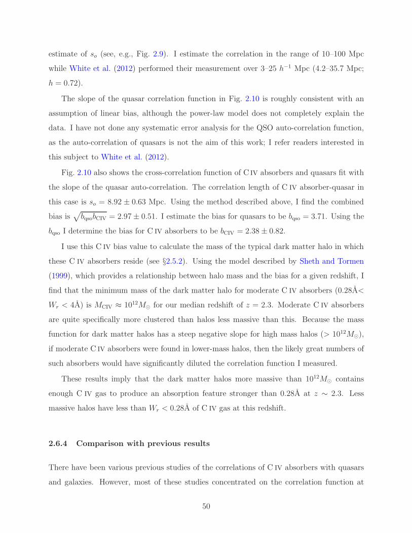
estimate of so (see, e.g., Fig. 2.9). I estimate the correlation in the range of 10–100 Mpc
while White et al. (2012) performed their measurement over 3–25 h−1 Mpc (4.2–35.7 Mpc;
h = 0.72).
The slope of the quasar correlation function in Fig. 2.10 is roughly consistent with an
assumption of linear bias, although the power-law model does not completely explain the
data. I have not done any systematic error analysis for the QSO auto-correlation function,
as the auto-correlation of quasars is not the aim of this work; I refer readers interested in
this subject to White et al. (2012).
Fig. 2.10 also shows the cross-correlation function of C IV absorbers and quasars fit with
the slope of the quasar auto-correlation. The correlation length of C IV absorber-quasar in
this case is so = 8.92 ± 0.63 Mpc. Using the method described above, I find the combined
bias is√
bqsobCIV = 2.97 ± 0.51. I estimate the bias for quasars to be bqso = 3.71. Using the
bqso I determine the bias for C IV absorbers to be bCIV = 2.38 ± 0.82.
I use this C IV bias value to calculate the mass of the typical dark matter halo in which
these C IV absorbers reside (see §2.5.2). Using the model described by Sheth and Tormen
(1999), which provides a relationship between halo mass and the bias for a given redshift, I
find that the minimum mass of the dark matter halo for moderate C IV absorbers (0.28A<
Wr < 4A) is MCIV ≈ 1012M for our median redshift of z = 2.3. Moderate C IV absorbers
are quite specifically more clustered than halos less massive than this. Because the mass
function for dark matter halos has a steep negative slope for high mass halos (> 1012M),
if moderate C IV absorbers were found in lower-mass halos, then the likely great numbers of
such absorbers would have significantly diluted the correlation function I measured.
These results imply that the dark matter halos more massive than 1012M contains
enough C IV gas to produce an absorption feature stronger than 0.28A at z ∼ 2.3. Less
massive halos have less than Wr < 0.28A of C IV gas at this redshift.
2.6.4 Comparison with previous results
There have been various previous studies of the correlations of C IV absorbers with quasars
and galaxies. However, most of these studies concentrated on the correlation function at
50

10 30 50 70 100
s Mpc10-2
10-1
100
(s)QSO-QSO
CIV-QSO
Figure 2.10 The quasar auto-correlation function (black circles). The green dashed line is
the best power law fit in the range of 10 Mpc< s < 100 Mpc. The redshift range for the
data is 2.1 < z < 2.5. The best-fit value for the power law is so = 12.19 ± 0.32 Mpc and
slope γ = 1.77 ± 0.04. The blue squares are the cross-correlation measurement for C IV
absorbers and quasars over this redshift range. The red dash-dot line is the best-fit value for
the correlation length, so = 8.92±0.63 Mpc, assuming a fixed slope derived from the quasar
auto-correlation.
51

much smaller distances than our study. Wild et al. (2008) quoted a correlation length of
so = 5.8 ± 1.1 h−1 Mpc with γ = −1.8 for C IV absorbers with rest-frame Wr >0.3A,
compared to our result of so = 6.09 ± 0.89h−1 Mpc (8.46 ± 1.46 Mpc; h = 0.72) with
slope γ = 1.68 ± 0.27, there is excellent agreement between results. Our measurement
more cleanly removes the intrinsic C IV absorbers for a correct measurement of correlation,
whereas Wild et al. (2008) modeled the intrinsic C IV absorbers and thus were reliant on
more assumptions.
The clustering of C IV absorbers and Lyman Break Galaxies(LBGs) was measured in
Adelberger et al. (2005) and Cooke et al. (2006) for CIV absorbers with rest-frame EW>0.4A
. Adelberger et al. (2005) measured the correlation length of CIV absorbers by comparing the
LBG auto-correlation and LBG-C IV cross-correlation to be ro ≈ 5±1h−1 Mpc (7±1.4 Mpc;
h = 0.72) at z ' 3. They also concluded that the C IV absorbers likely formed in these
early large galaxies rather than in some more distributed environment. Our study from
10 Mpc< rp < 100 Mpc is 1σ consistent with this result (ro = 7.76± 2.8). Our study covers
a much larger redshift range and has significantly greater statistical power due to the larger
number of absorbers.
Our results corroborate the idea that LBG and C IV absorbers, having similar clustering
properties, reside in similar environments and the same dark matter potentials.
2.7 SYSTEMATIC UNCERTAINTIES
In this section I discuss potential systematic uncertainties in our measurement presented in
§2.6.
2.7.1 North Galactic Cap vs Full Sample
I explore a potential systematic difference between the North Galactic Cap (NGC) and South
Galactic Cap (SGC) data set. The NGC portion of BOSS footprint is much larger than the
SGC portion, which makes the correlation function for SGC alone very noisy. To explore
52
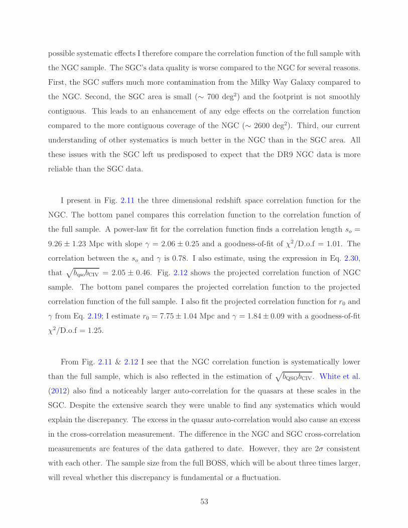
possible systematic effects I therefore compare the correlation function of the full sample with
the NGC sample. The SGC’s data quality is worse compared to the NGC for several reasons.
First, the SGC suffers much more contamination from the Milky Way Galaxy compared to
the NGC. Second, the SGC area is small (∼ 700 deg2) and the footprint is not smoothly
contiguous. This leads to an enhancement of any edge effects on the correlation function
compared to the more contiguous coverage of the NGC (∼ 2600 deg2). Third, our current
understanding of other systematics is much better in the NGC than in the SGC area. All
these issues with the SGC left us predisposed to expect that the DR9 NGC data is more
reliable than the SGC data.
I present in Fig. 2.11 the three dimensional redshift space correlation function for the
NGC. The bottom panel compares this correlation function to the correlation function of
the full sample. A power-law fit for the correlation function finds a correlation length so =
9.26 ± 1.23 Mpc with slope γ = 2.06 ± 0.25 and a goodness-of-fit of χ2/D.o.f = 1.01. The
correlation between the so and γ is 0.78. I also estimate, using the expression in Eq. 2.30,
that√
bqsobCIV = 2.05 ± 0.46. Fig. 2.12 shows the projected correlation function of NGC
sample. The bottom panel compares the projected correlation function to the projected
correlation function of the full sample. I also fit the projected correlation function for r0 and
γ from Eq. 2.19; I estimate r0 = 7.75± 1.04 Mpc and γ = 1.84± 0.09 with a goodness-of-fit
χ2/D.o.f = 1.25.
From Fig. 2.11 & 2.12 I see that the NGC correlation function is systematically lower
than the full sample, which is also reflected in the estimation of√
bQSObCIV. White et al.
(2012) also find a noticeably larger auto-correlation for the quasars at these scales in the
SGC. Despite the extensive search they were unable to find any systematics which would
explain the discrepancy. The excess in the quasar auto-correlation would also cause an excess
in the cross-correlation measurement. The difference in the NGC and SGC cross-correlation
measurements are features of the data gathered to date. However, they are 2σ consistent
with each other. The sample size from the full BOSS, which will be about three times larger,
will reveal whether this discrepancy is fundamental or a fluctuation.
53

101 102
s(Mpc)
2.52.01.51.00.5
0.00.51.01.52.0
NGC(s)(s)(s)
10-2
10-1
100
(s)NGC 3d cross-correlation(4724)
Figure 2.11 The redshift space correlation function of CIV absorbers and quasars in the NGC.
The dotted line is the best fit power-law, as defined in Eq. 2.18,with so = 9.26 ± 1.23 Mpc
and slope γ = 2.06 ± 0.25 in the range 10 < s < 100 Mpc. The redshift range for the C IV
absorber and quasar is 2.1 < z < 2.5 . The lower panel compares the NGC correlation
function to the full sample correlation function.
54

101 102
rp (Mpc)
1.5
1.0
0.5
0.0
0.5
1.0
wp,NGC
w pw p 101 102
rp (Mpc)
10-3
10-2
10-1
100
wp/r p
NGC projected correlation(4724)
Figure 2.12 Projected correlation function for C IV absorbers and quasars in the NGC. The
dashed line is the best fit power-law, as defined in Eq. 2.19 and 2.20, with r0 = 7.76±3.80 Mpc
and slope γ = 1.74 ± 0.21 in the range 10 Mpc< wp < 100 Mpc in the redshift range of
2.1 < z < 2.5. The lower panel compares the NGC projected correlation function to the full
sample one.
55
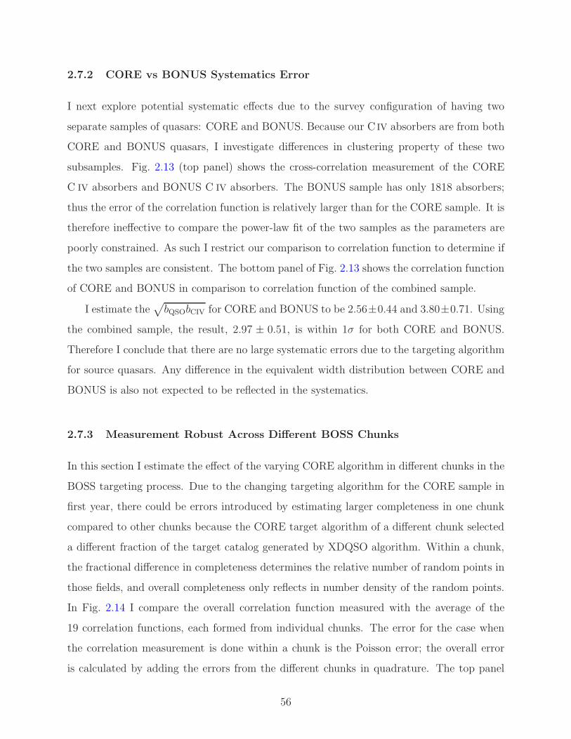
2.7.2 CORE vs BONUS Systematics Error
I next explore potential systematic effects due to the survey configuration of having two
separate samples of quasars: CORE and BONUS. Because our C IV absorbers are from both
CORE and BONUS quasars, I investigate differences in clustering property of these two
subsamples. Fig. 2.13 (top panel) shows the cross-correlation measurement of the CORE
C IV absorbers and BONUS C IV absorbers. The BONUS sample has only 1818 absorbers;
thus the error of the correlation function is relatively larger than for the CORE sample. It is
therefore ineffective to compare the power-law fit of the two samples as the parameters are
poorly constrained. As such I restrict our comparison to correlation function to determine if
the two samples are consistent. The bottom panel of Fig. 2.13 shows the correlation function
of CORE and BONUS in comparison to correlation function of the combined sample.
I estimate the√
bQSObCIV for CORE and BONUS to be 2.56±0.44 and 3.80±0.71. Using
the combined sample, the result, 2.97 ± 0.51, is within 1σ for both CORE and BONUS.
Therefore I conclude that there are no large systematic errors due to the targeting algorithm
for source quasars. Any difference in the equivalent width distribution between CORE and
BONUS is also not expected to be reflected in the systematics.
2.7.3 Measurement Robust Across Different BOSS Chunks
In this section I estimate the effect of the varying CORE algorithm in different chunks in the
BOSS targeting process. Due to the changing targeting algorithm for the CORE sample in
first year, there could be errors introduced by estimating larger completeness in one chunk
compared to other chunks because the CORE target algorithm of a different chunk selected
a different fraction of the target catalog generated by XDQSO algorithm. Within a chunk,
the fractional difference in completeness determines the relative number of random points in
those fields, and overall completeness only reflects in number density of the random points.
In Fig. 2.14 I compare the overall correlation function measured with the average of the
19 correlation functions, each formed from individual chunks. The error for the case when
the correlation measurement is done within a chunk is the Poisson error; the overall error
is calculated by adding the errors from the different chunks in quadrature. The top panel
56

101 102
s(Mpc)
32101234
bonusorcore(s)
(s)(s)
10-2
10-1
100
(s)CORE CIV-QSO(4331)
BONUS CIV-QSO(1818)
Figure 2.13 Cross-Correlation for the CORE C IV absorbers and BONUS C IV absorbers (top
panel). The two correlation functions are consistent with each other, but the large errors
would mask all but very large differences. The bottom panel compares the both sample
correlation functions to the combined correlation function.
57

displays the correlation functions ξchunk(s) and ξ(s). The bottom panel is the difference of
the correlation calculated within chunk ξchunk and the overall correlation function in units
of the Jackknife error of the overall correlation function. If there is a systematic error from
the chunking process and evolving CORE algorithm, I would expect either consistently more
than the correlation calculated within chunks or consistently less, caused by different overall
levels of completeness, due to different algorithm used in different chunks. However, it is not
clear the plot signifies any trend of the ξchunk being consistently either more or less than the
overall estimate of correlation function, which indicates that is there is no large effect from
the use of slightly different selection algorithms in different BOSS chunks.
For the chunk correlation function I estimate√
bqsobCIV = 2.07 ± 0.61 but the error is
larger compared to combined sample. The correlation function does not appear to be biased
compared to the combined sample. For the full BOSS sample the problem will be irrelevant
as all subsequent chunks will use the same target selection algorithm. All the coverage will
fill the space in the foot print and significantly reduce any edge effects.
2.7.4 Other Systematic Errors
In this section I estimate the systematic effect of various properties of the sample on the
estimates of the correlation strength (r0), the slope (γ), and the bias of C IV absorbers
and quasars√
bCIVbQSO. The errors on our parameters are large, and the samples are
not sufficiently large to perform the typical systematic analysis in which one calculates
the correlation function for a bin for each parameter space and measure the change in the
correlation function in every bin. Hence, I used a jackknife procedure because it works well
on small samples. To estimate each systematic, I compared the Jackknife error caused by
dividing the sample into bins based on a ordering in the given parameter to the Jackknife
errors from a random division of the data in to same number of bins. The Jackknife error
brings out the systematic error for the parameter in consideration. The significance of this
is estimated by dividing the sample randomly and get the distribution of Jackknife error.
Below is the specific procedure I follow:
1. Sort the C IV absorbers according to the given property (e.g., equivalent width).
58
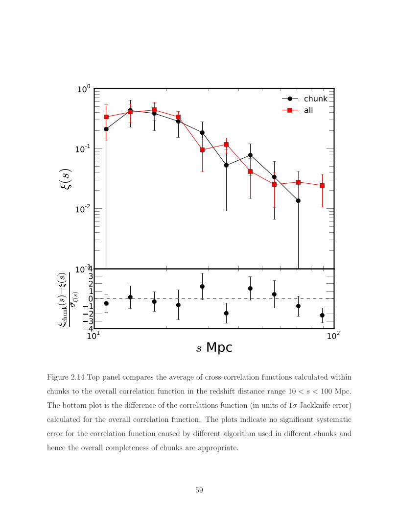
101 102
s Mpc
432101234
chunk(s)
(s)(s)10-3
10-2
10-1
100
(s)chunk
all
Figure 2.14 Top panel compares the average of cross-correlation functions calculated within
chunks to the overall correlation function in the redshift distance range 10 < s < 100 Mpc.
The bottom plot is the difference of the correlations function (in units of 1σ Jackknife error)
calculated for the overall correlation function. The plots indicate no significant systematic
error for the correlation function caused by different algorithm used in different chunks and
hence the overall completeness of chunks are appropriate.
59

2. Calculate the jackknife error by dividing the C IV absorber sample, according to property
in consideration, into 10 bins for r0, γ and√
bCIVbQSO .
3. Calculate the jackknife error by dividing the C IV absorber sample, randomly, into 10
bins for r0, γ and√
bCIVbQSO .
4. Do the previous step 5,000 times and find the distribution of r0, γ, and√
bCIVbQSO.
5. Estimate the probability of measured Jackknife error by random chance, called p-value
by using of the distribution of the random scatter of errors in previous step.
Following the above procedure, I explore the systematic effects of absorber equivalent
width, β, i-band magnitude, absorber redshift, quasar spectroscopic features, and Galactic
latitude. Table 2.4 summarizes the mean variation and standard deviation of the parameters
for each systematic. Fig 2.15, 2.16, and 2.17 show the distribution of the parameters r0, γ
and√
bCIVbQSO from the random jackknifing of the sample. Below I describe each systematic
and its potential effect on the correlation function measurements. In many cases a systematic
error of one property could be correlated with that of another.
1. Absorber Equivalent Width: There are two obvious ways the equivalent width of
the C IV absorber could affect the systematic error.
A) There could be a few false positive C IV absorbers in the sample, and such con-
tamination may not be distributed uniformly across the equivalent width distribution.
The lower equivalent width absorbers are more likely to be contaminated by false pos-
itives compared to the high equivalent absorbers. This contamination will decrease the
correlation strength for lower equivalent width absorbers.
B) There could also be an intrinsic correlation dependence on equivalent-width. The
higher equivalent-width absorbers could be more correlated with dark matter compared
to lower equivalent-width absorbers. However, our error estimations of the correlation
function are not small enough to measure this trend.
Following our systematic analysis, I found a noticeable, but not statistically significant,
increase in the change in bias as different equivalent-width bins are dropped. The prob-
ability of having such error occuring by chance is 13%.
2. β: The CIV absorber sample could have two basic origins. One may be intrinsic to quasars
60
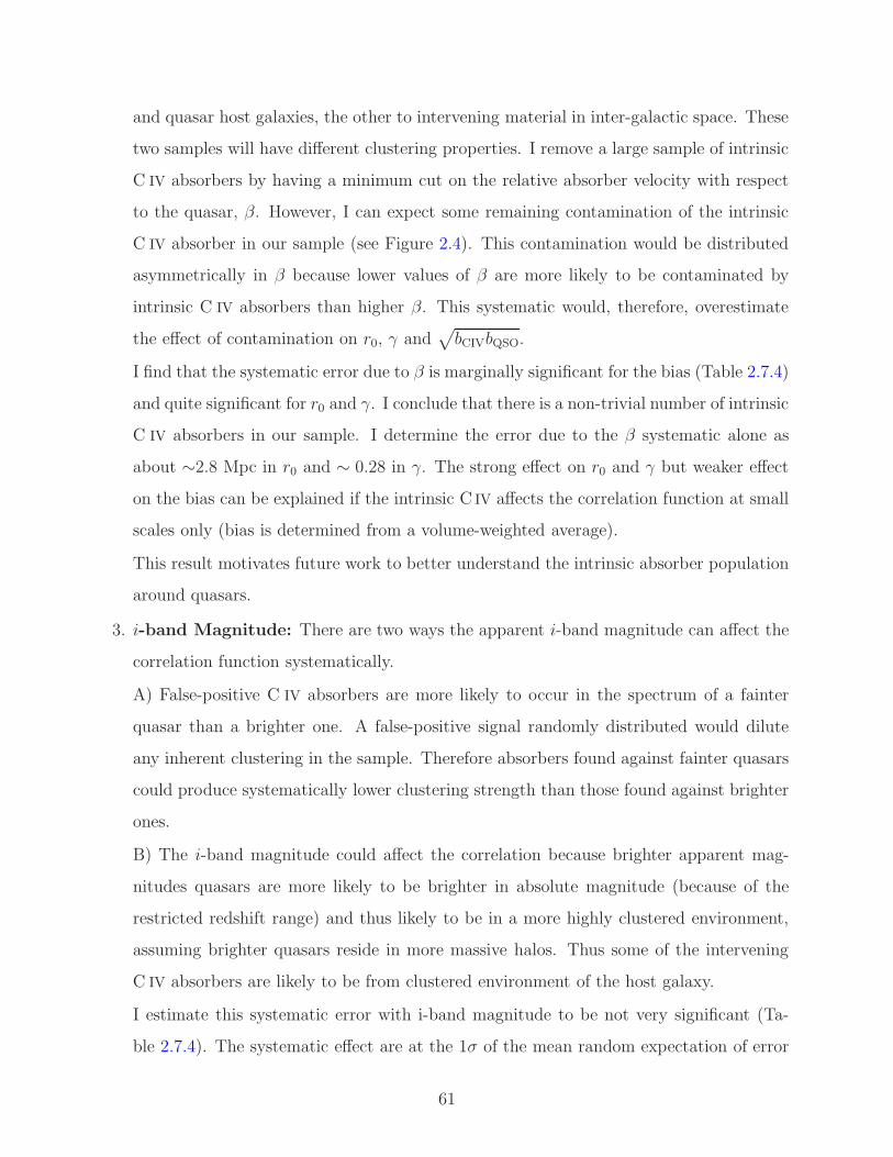
and quasar host galaxies, the other to intervening material in inter-galactic space. These
two samples will have different clustering properties. I remove a large sample of intrinsic
C IV absorbers by having a minimum cut on the relative absorber velocity with respect
to the quasar, β. However, I can expect some remaining contamination of the intrinsic
C IV absorber in our sample (see Figure 2.4). This contamination would be distributed
asymmetrically in β because lower values of β are more likely to be contaminated by
intrinsic C IV absorbers than higher β. This systematic would, therefore, overestimate
the effect of contamination on r0, γ and√
bCIVbQSO.
I find that the systematic error due to β is marginally significant for the bias (Table 2.7.4)
and quite significant for r0 and γ. I conclude that there is a non-trivial number of intrinsic
C IV absorbers in our sample. I determine the error due to the β systematic alone as
about ∼2.8 Mpc in r0 and ∼ 0.28 in γ. The strong effect on r0 and γ but weaker effect
on the bias can be explained if the intrinsic C IV affects the correlation function at small
scales only (bias is determined from a volume-weighted average).
This result motivates future work to better understand the intrinsic absorber population
around quasars.
3. i-band Magnitude: There are two ways the apparent i-band magnitude can affect the
correlation function systematically.
A) False-positive C IV absorbers are more likely to occur in the spectrum of a fainter
quasar than a brighter one. A false-positive signal randomly distributed would dilute
any inherent clustering in the sample. Therefore absorbers found against fainter quasars
could produce systematically lower clustering strength than those found against brighter
ones.
B) The i-band magnitude could affect the correlation because brighter apparent mag-
nitudes quasars are more likely to be brighter in absolute magnitude (because of the
restricted redshift range) and thus likely to be in a more highly clustered environment,
assuming brighter quasars reside in more massive halos. Thus some of the intervening
C IV absorbers are likely to be from clustered environment of the host galaxy.
I estimate this systematic error with i-band magnitude to be not very significant (Ta-
ble 2.7.4). The systematic effect are at the 1σ of the mean random expectation of error
61

and the p-value similarly indicates no significant deviation from random chance.
4. Absorber Redshift: The potential systematic effect of contamination because of false
positives due to potential incomplete sky subtraction in the BOSS quasar spectra is
minimal in this analysis. A sky line at a particular wavelength would affect the C IV
absorbers at a particular absorber redshift. Any sky line which falls in the observed
wavelength range for a given redshift range for C IV absorbers could contribute to a
reduced signal in this range. Such contamination would possibly lead to smaller clustering
measurement which would lead to systematic error. However, the strong O I sky line
5570-5590A is removed from the absorber pipeline, which corresponds to C IV absorber
redshift of 2.59. Our cutoff absorber redshift of 2.5 avoids any neighboring part of
spectrum which might be affected.
With this motivation in mind for potential lines I may have neglected in the above cut,
I searched for a dependence of our fit parameters on the absorber redshift. However, I
found no significant systematic effect (Table 2.7.4). Hence I expect that the sky subtrac-
tion for the relevant region of the spectrum is sufficient and no sky-line-contamination
creates false C IV absorber detections.
5. Galactic Latitude: The extinction through the Milky Way varies with galactic latitude.
Such extinction could be correlated to poor signal-to-noise and could lead to false positive
detection of C IV absorbers. The Galactic latitude could also potentially interact with
the cosmic variance error along with contamination effect on correlation function. Hence
the estimate of error could be overestimating error because of contamination.
Table 2.7.4 shows the significance of the systematic error due to Galactic latitude in
bias. This is another way of looking at the NGC vs. SGC discrepancy discussed in
2.7.1. I estimate the error due to Galactic latitude on√
bCIVbQSO to be 0.494 with < 3%
probability of such a shift occuring by chance.
6. Quasar Redshift: The biggest potential systematic from quasars at different redshifts
(beyond any apparent magnitude variation as explored above) is a potential systematic
contamination associated with features in the quasar spectrum, which could lead to a
false positive identification as a C IV absorber. These contaminating lines would affect
the correlation function asymmetrically at different rest frame wavelengths. However,
62

Table 2.3. Systematic error estimates and p-values for r0, γ and√
bCIVbQSO.
Description δr0 δγ δ√
bCIVbQSO
Equivalent Width 2.562 0.306(0.424) 0.477(0.130)
β 3.875(0.027) 0.405(0.051) 0.424(0.298)
i-band Magnitude 3.344(0.140) 0.335(0.266) 0.351
Absorber Redshift 2.574 0.258 0.412(0.346)
Galactic Latitude 3.300(0.157) 0.335(0.270) 0.618(0.003)
Quasar rest frame λ a 3.874(0.027) 0.404(0.052) 0.415(0.331)
aThe absorber redshift, β, and quasar rest frame are three differ-
ent representations of only two independent quantities.
this systematic error actually becomes strongly correlated with the β systematic error
because the absorbers that are near particular quasar rest-frame wavelengths also fall
into specific β range. I indeed find very similar dependence between β and the quasar
redshift as shown in Table 2.7.4.
Table 2.4 Random error distribution for r0, γ and√
bCIVbQSO.
Parameter mean std dev
δr0 2.667 0.628
δγ 0.293 0.068
δ√
bCIVbQSO 0.376 0.089
63
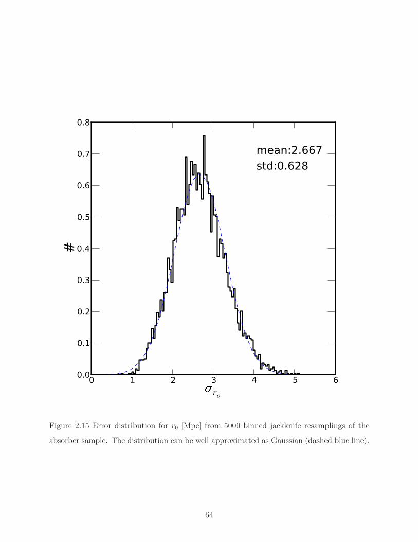
0 1 2 3 4 5 6ro0.0
0.1
0.2
0.3
0.4
0.5
0.6
0.7
0.8
#
mean:2.667std:0.628
Figure 2.15 Error distribution for r0 [Mpc] from 5000 binned jackknife resamplings of the
absorber sample. The distribution can be well approximated as Gaussian (dashed blue line).
64

0.0 0.1 0.2 0.3 0.4 0.5 0.60
1
2
3
4
5
6
7
#
mean:0.293std:0.068
Figure 2.16 Error distribution for γ from 5000 binned jackknife resamplings of the absorber
sample. The distribution can be well approximated as Gaussian (dashed blue line).
65

0.1 0.2 0.3 0.4 0.5 0.6 0.7 0.8 bcivbqso0
1
2
3
4
5
#
mean:0.376std:0.089
Figure 2.17 Error distribution for√
bCIVbQSO from 5000 binned jackknife resamplings of the
absorber sample. The distribution can be well approximated as Gaussian (dashed blue line).
66
2.8 SUMMARY AND FUTURE DIRECTIONS
This study has measured the correlation strength of C IV absorbers with the quasars from
the BOSS survey. I focus on correlations between 10 Mpc< s < 100 Mpc at z ∼ 2.3, probing
the large-scale clustering unaffected by details of the astrophysics of the galaxy environment
surrounding quasars. I conclude the following:
• The three-dimensional two-point cross-correlation for C IV absorbers and quasars is well
approximated by a power law in the distance range 10 < s < 100 Mpc with s0 =
8.46 ± 1.46 Mpc and γ = 1.68 ± 0.27.
• The projected cross-correlation for C IV absorbers and quasars is well approximated by
a power law in the distance range 10 < rp < 100 Mpc with r0 = 7.76 ± 3.80 Mpc and
γ = 1.74 ± 0.21.
• I measure the combined QSO-C IV absorber bias√
bqsobCIV = 2.97 ± 0.51.
• I estimate the quasar auto-correlation and find a correlation length so = 12.19±0.32 Mpc
and slope γ = 1.77 ± 0.04 and thus infer a quasar bias of bqso = 3.71.
• Using this estimate of the quasar bias bqso I find bCIV = 2.38±0.82 and that EW> 0.28A
C IV absorbers reside in halos of mass MCIV ≥ 1012M.
• The dominant sources of systematic error in our estimation of CIV absorber bias are (1) a
difference as a function Galactic latitude (NGC vs. SGC; §2.7.1); (2) absorber equivalent
width; and (3) potential contamination of high-velocity intrinsic-absorbers (β > 0.2).
This study lays the groundwork for subsequent work of both improved clustering analysis
with an extended data set, as well as enabling complementary approaches to investigate
C IV absorbers. With the well-constrained correlation of C IV absorbers at cosmological
separations, one can propagate the two-halo correlation function down to small scales to
remove this contribution from low-β absorbers, enabling a cleaner investigation of C IV
absorbers in the same halo as the quasars. Any departure from the expected number of C IV
would indicate the role of quasars in creating/destroying the absorbers, leading to a better
understanding of quasars.
67

A repeated analysis with the full BOSS sample will not only have ∼3 times more quasars
and absorbers, but will also will have significantly reduced edge effects and have a more
uniform completeness and coverage. The question of any NGC vs. SGC difference (currently
consistent with Poisson fluctuations) will be settled, and with a cleaner sample of quasars
and absorbers it will be possible to make a random catalog for CIV absorbers without having
to assume a specific redshift dependence of the their number density. The increased number
of absorbers will also allow us to measure the correlation function as a function of equivalent
width and other absorber properties. The final SDSS-III BOSS C IV absorber analysis will
feature improved systematic errors and more clearly highlight the statistical power of these
large samples.
68

3.0 QUASAR OUTFLOWS USING INTRINSIC ABSORPTION SYSTEMS
In §1.3 I presented an overview of quasars and their utility. I introduced the idea of using
absorption systems to study the structure of quasars. In this chapter, I study the outflows
in quasars using C IV absorbers seen in the spectra of SDSS-III BOSS quasars from DR9.
In §3.1, I describe the motivation behind, and the importance of, this study. In §3.2, I
present the models for the data and explain the reasoning behind them. In §3.3, I explain
the halo occupation formalism, which is used as the guiding principle for the estimation of
the correlation function. In §3.4, I present the observational data used for this study. In
§3.5, I explain the estimation of the correlation function required for the models. In §3.6,
I present the result of the analysis and interpretation. In the last section, §3.7, I present a
summary of this analysis and comment on future directions for this study.
3.1 MOTIVATION
Quasars can be identified during the epoch when galaxies were assembling and the star
formation rate was ten times higher than today. Because they are a biased tracer of high
density environments in the early universe, understanding quasars can help in understanding
the formation of large scale structure and the formation and evolution of galaxies. Being
very energetic, quasars can be powerful engines that mix material within a galaxy as well as
expell material into the Inter Galactic Medium (IGM). Such feedback processes have been
postulated to reduce the growth of baryonic structure in the early universe (Silk and Rees
1998; Springel et al. 2005; Di Matteo et al. 2005; Bower et al. 2006). Therefore understand-
ing quasars and their outflows is an important route to correctly explain the formation of
69

stars and the distribution of elements in and around galaxies.
Many models of quasar outflows postulate that the gas arises from the accretion disk. But
we still do not know how these flows are launched. There have been many models explaining
their origin and how they are ejected from the inner region. Some models use only line
radiation pressure (Arav et al. 1994; Murray et al. 1995; Proga et al. 2000) while others add
in magnetic forces (de Kool and Begelman 1995; Everett 2005; Proga and Kallman 2004) to
accelerate the material.
Despite their importance, the understanding of quasars is fairly limited due to their ex-
treme distance and extreme physics. Many studies have been done to understand quasar
outflows from the broad absorption lines (BALs) (e.g., Weymann et al. 1979; Yuan and Wills
2003; Richards 2006; Ganguly et al. 2007; Lundgren et al. 2007). The BALs are unambigu-
ously associated with quasars which make them easy targets for detailed study. There have
been other studies using narrow absorption lines (NALs) to study the outflows of quasars
(Foltz et al. 1988; Aldcroft et al. 1994; Ganguly et al. 2001; Baker et al. 2002; Vestergaard
2003; Richards 2001; Misawa et al. 2007; Ganguly et al. 2007). The study of NALs has many
advantage over BALs. Most notably the NALs are detected in a large fraction of quasars (∼50%) compared to BALs (∼ 10%). And unlike BALs, NALs do not suffer from line blending.
However NALs do suffer from one important disadvantage: NALs are produced by the
intervening galaxies along the line of sight as well. Hence identifying the NAL to be intrinsic
to the quasar is often a very difficult task. However a large fraction of the NALs having a
redshift similar to the quasar redshift are likely intrinsic. But these can still have significant
velocities with respect to the quasar. For example, Richards (2001) suggests that ∼36% of
NALs with a velocity with respect to the quasar rest frame of v > 5000 km/s are intrinsic,
i.e., physically close in distance to the quasar.
NALs also provide a complementary study of quasars compared to BALs. As the BAL
gas clouds are believed to be closer to the accretion disk and NAL gas clouds are much
further, they probe different parts of a quasar and together, may offer a more complete
picture of the quasar and the surrounding environment.
70

3.2 NUMBER DENSITY OF C IV ABSORBERS
The light from a quasar travels through its own dark matter halo and other halos picking
up signatures of the absorption systems encountered. The frequency of such encounters is
determined by the number density of the absorption systems. Figure 3.1 shows a schematic
diagram of a sample line of sight from a quasar to an observer. In this section I model
the observed frequency of absorption systems detected in the rest-frame of the backlighting
quasars. Motivated by the different physical origins of the absorption systems, I divide the
absorbers into three broad categories: 1. in the host halo due to clustering (one halo); 2. in
an intervening halo (two halo); 3. in the outflowing gas due to quasar environment (outflow).
The total probability of an absorption system can now be written as
d P = d P 1h + d P 2h + d P outflow (3.1)
I use separate models for describing each separate component.
• Two-halo d P : We are going to first evaluate the d P 2h term. For this component the
absorption systems are not very close to the quasar in velocity space. In the pencil beam
survey the probability of detecting an absorber between z and z + d z is given as (e.g.,
Hogg 1999)
d P 2h = n(z)σ(z)c
Ho
(1 + z)2
√
ΩM(1 + z)3 + ΩΛ
d z (3.2)
where n(z) and σ(z) are the number density and cross section respectively of C IV ab-
sorbers at redshift z. ΩM , ΩΛ, Ho are the relevant cosmological parameters. Modeling
the redshift dependence of n(z) as a correlation of quasars and C IV absorbers we can
write
n(z)σ(z) = noσo(1 + ξ2h(r; zqso))(1 + z)ε (3.3)
where ε characterizes the evolution of number density with redshift and noσo is the
current value of number density and cross-section. ξ2h(r; zqso) is the cross-correlation
function of quasars and C IV absorbers from different halos. Note that the ξ in the
equation indicates that matter in the universe is clustered and hence, even with no
71

intrinsic physical connection, there are more C IV absorbers near quasars compared to
further away.
Since we are interested in outflow velocities from the quasar, it is logical to do the analysis
in the velocity space of the quasar rest-frame. I convert probabilities in redshift space to
probabilities in quasar rest-frame velocity space, β, using the following relationships
β ≡ v
c=
(1 + zqso)2 − (1 + z)2
(1 + zqso)2 + (1 + z)2(3.4)
and
d β ≡ d v
c= − 4 (1 + z) (1 + zqso)2 d z
[
(1 + zqso)2 + (1 + z)2]2
. (3.5)
This leads to an expected probability of C IV absorbers from intervening DM halos of
d P
d β
2h
(zqso) = noσo(1 + ξ2h(r; zqso))c
hHo
(1 + z)1+ε
√
Ωm(1 + z)3 + ΩΛ
[
(1 + zqso)2 + (1 + z)2]2
4(1 + zqso)2
(3.6)
• One-halo d P : For the single halo term I assume that the host halo is virialized. So the
velocity of an absorption system in the rest-frame of quasar can be well approximated
as a Gaussian
p(v) d v =1
√
2πσ2v
exp
(
− v2
2σ2v
)
. (3.7)
Hence, for the single halo term we can write the probability of observation as
d P
d β
1h
(zqso) =f√2π
exp
(
− β2
2σ2β
)
(1 + zqso)ε (3.8)
Here we assume that the average number of absorbers in a halo evolves as (1 + zqso)ε.
The parameters unknown in the above equation are f , σβ.
• Outflow d P : The outflow term is modeled as a piece-wise continuous function described
by
d P outflow
d v=
n2k/2000 0 < v < 2000 km/s
(n4k − n2k)/2000 2000 < v < 4000 km/s
(n6k − n4k)/2000 4000 < v < 6000 km/s
−n6k/2000 6000 < v < 8000 km/s
0 v < 0 km/s&v > 8000 km/s
(3.9)
72

The simple piece-wise function is considered appropriate as it makes the fewest assump-
tions about the shape of the outflow distribution while at the same time having only
a small number of free parameters. The velocity range of the function is chosen to be
0-8000 km/s because in tests of this range any free parameter greater than 8000 km/s
was found to be consistent with zero.
In the SDSS-III BOSS DR9 sample the redshift of the quasar, zqso, is uncertain due to the
astrophysical variation of different emission line velocities. Hence the measured value of the
number of absorbers in a bin between r and r +d r will be a convolution of the redshift error
of the quasar with the actual number density of absorbers. We can not observe absorption
lines at all possible redshifts; we can only observe the absorbers that are physically between
us and the quasars. Also, a quasar spectrum observed from the ground can only detect C IV
absorption redward of the UV. Therefore, for every quasar at redshift zqso there is a minimum
zmin(zqso) and maximum redshift zmax(zqso) at which we can observe a CIV absorption system
in the SDSS-III BOSS data.
Hence the observed number density from all quasars can be given as
d P
d β
∣
∣
∣
∣
observable
= Gaussian(0, σz) ∗∑
qso
d P
d β(zqso)H(z − zmin(zqso))H(zmax(zqso) − z) (3.10)
where H , zmax, and zmin are the Heaviside Step Function, maximum redshift, and minimum
redshift respectively.
3.3 CORRELATION FUNCTIONS IN A HALO MODEL FRAMEWORK
Halo models are a formalism to describe the clustering of objects. The formalism has a
long history and has provided important analytical descriptions of large scale clustering
(Neyman and Scott 1952; McClelland and Silk 1977a,b; Peebles 1974). After the realization
that most matter in the universe is in the form of dark matter which interacts only gravita-
tionally, the halo formalism was further developed to provide an analytical tool for predicting
clustering of dark matter halos (Mo and White 1996; Sheth and Tormen 1999; Sheth et al.
73

Figure 3.1 A cartoon description of a line of sight from a quasar (left) to an observer (right).
The big circles indicate the dark matter halos. The arrows shows the uncertainty in location
due to peculiar velocities within the host halos.
2001; Seljak and Warren 2004; Tinker et al. 2005). These models developed for dark matter
halos are easily extensible for studies of the clustering of any population.
3.3.1 Basics of The Halo Model Formalism
The halo model formalism is based on a few assumptions. One of the basic assumptions is
that all matter resides in halos of different sizes. The size distribution of halos is given by the
mass function, denoted by d n/ d M (e.g., Sheth and Tormen (1999); Jenkins et al. (2001)).
The mass function is the number of dark matter halos of mass between M and M + d M
in a comoving unit volume. The halo bias is bh(M) is defined as the overdensity of halo of
mass between M and M + d M compared to the overdensity of all matter (Efstathiou et al.
1988; Mo and White 1996; Jing 1998; Sheth and Tormen 1999). The distribution of dark
matter within a halo is described by the density profile around the center of the halo as
λ(r|M) (Navarro et al. 1997; Bullock et al. 2001a). These ingredients are estimated using
dark matter simulations or approximate analytical solutions.
Using the ingredients of the halo model formalism we can calculate the clustering of
74

any kind of object or of different types of objects. Here I estimate the two-point correlation
function of C IV absorbers and quasars using the halo model formalism below. The two-point
correlation function describes the clustering of C IV absorber and quasar pairs as a function
of the distance between them. Any pair of C IV absorber and a quasar can be of either of two
origins; 1) both reside in the same halo, called the one-halo term or, 2) reside in different
halo, called the two-halo term. The total correlation function is the sum of these two and
can be written as follows.
ξqso,CIV(r) = ξ1hqso,CIV(r) + ξ2h
qso,CIV(r) (3.11)
where ξ1hqso,CIV(r) is the one-halo correlation term and ξ2h
qso,CIV(r) is the two-halo term. These
two terms can be calculated separately (Scherrer and Bertschinger 1991). The one halo term
is written as
ξ1hqso,CIV(r) = n−1
qson−1CIV
∫
d Md n
d M〈NqsoNCIV〉(M)
∫
d3 ~xλ(~x|M)λ(~x + ~r|M). (3.12)
where nqso and nCIV are the average number density of quasars and C IV absorbers, respec-
tively. 〈NqsoNCIV〉(M) is the average of the number of quasars times the number of C IV
absorbers in halos of mass between M and M + d M .
Similarly, the two-halo term can be written as follows.
ξ2hqso,CIV(r) = n−1
qson−1CIV
∫
d Md n
d M〈Nqso〉(M)
∫
d M ′d n
d M ′〈NCIV〉(M ′)
×∫
d3 ~x
∫
d3 ~yλ(~x|M)λ(~y|M ′)ξhh(~x − ~y − ~r|M, M ′)
(3.13)
where 〈Nqso〉(M) and 〈NCIV〉(M) are the average number of quasars and C IV absorbers
respectively, in the halos of mass between M and M + d M , and ξhh(M, M ′) is the two-point
cross-correlation function of dark matter halos of mass M with those of mass M ′.
For our analysis we will be required to calculate only ξ2hqso,CIV(r) and not ξ1h
qso,CIV(r). The
two halo term can further be simplified by assuming ξhh(r|M, M ′) ' bh(M)bh(M ′)ξlinDM(r),
75

where ξlinDM is the dark matter power spectrum in linear perturbation theory. Using this
assumption the two-halo cross-correlation function can be written as
ξ2hqso,CIV(r) = n−1
qson−1CIV
∫
d Md n
d M〈Nqso〉(M)bh(M)
∫
d M ′d n
d M ′〈NCIV〉(M ′)bh(M ′)
×∫
d3 ~x
∫
d3 ~yλ(~x|M)λ(~y|M ′)ξlinDM(~x − ~y − ~r|M, M ′)
(3.14)
It is often helpful to take the Fourier transform of an equation that involves convolution
as the convolution in real space become simple multiplication in Fourier space. We can write
the above equation in Fourier space as follows.
P 2hqso,CIV(k) = n−1
qson−1CIVP lin(k)
∫
d Md n
d M〈Nqso〉(M)λ(k|M)
×∫
d M ′d n
d M ′〈NCIV〉(M ′)λ(k|M ′)
(3.15)
where n is defined as
n =
∫
d Md n
d M〈N〉 (3.16)
3.3.2 Mass Function and Bias
The equations in the halo model formalism are generally written in term of the variable
ν ≡ δc(z)/σ(M), where δc(z) is the equivalent linear collapse overdensity and σ(M) is the
rms mass fraction in the linear density field smoothed on a scale containing mass M . The
quantity f(ν) d ν denotes the fraction of mass contained in halos in a range d ν about ν.
Then the mass function is related to f(ν) by
d n
d M= 2ν2f(ν)
( ρ
M
) d ln ν
d M. (3.17)
Using the above equation we can write
P 2hqso,CIV(k) = P lin(k)bqso(k)bCIV(k), (3.18)
where b(k) can be written as
b(k) =
∫
d ln(ν)ν2f(ν)bh(ν)λ(k|ν)〈N〉(M)∫
d ln(ν)ν2f(ν)〈N〉(M). (3.19)
76

There are many different mass functions which are derived from analytical and dark mat-
ter simulations (Press and Schechter 1974; Sheth et al. 2001; Jenkins et al. 2001; Tinker et al.
2010). Here we use the mass function and halo bias from Sheth et al. (2001) which is based
on a model of ellipsoidal collapse of dark matter. The mass function of Sheth-Tormen is
given by
f(ν) = A(p)
√
2a
π
(
1 +1
(√
aν)2p
)
ν exp(−aν2/2) (3.20)
where a = 0.707, p = 0.3, and A(p) = [1 + 2−pΓ(0.5 − p)/√
π] ≈ 0.3222. The halo bias for
the Sheth-Torman mass function is given by
bh(ν) = 1 +aν2 − 1
δc
+2p/δc
1 + (aν2)p. (3.21)
To make further progress we need to make some assumption about 〈Nqso〉(M) and 〈NCIV〉(M).
We are assuming 〈N〉(M) to be of some functional form.
3.3.3 Density profiles of Halos
There are many studies that have attempted to determine the density profile of dark matter
halos (Hernquist 1990; Navarro et al. 1997; Moore et al. 1999). The NFW profile proposed
by Navarro et al. (1997) is the most commonly used dark matter profile. We are going to
assume the NFW profile for our studies which is given as
λ(r|M) =ρs
(
rrs
)(
1 + rrs
)2 (3.22)
where ρs and rs are model parameters. A more frequent parametrization is the concentration
parameter which is defined as c ≡ rvir/rs. Dark matter simulations, show that for halos of
the same mass, the distribution of the concentration parameter is given by a log-normal
distribution (Jing 2000; Bullock et al. 2001b).
p(c|M, z) d c =d ln c
√
2πσ2ln c
exp
(
− ln2 c/c(M, z)
2σ2ln c
)
(3.23)
77

where σln c ≈ 0.25 and c(M, z) ok given by
c(M, z) =9
1 + z
(
M
M?(z)
)−0.13
, (3.24)
where M?(z) is the characteristic mass at which ν(M, z) = 1. The mass of the halo can be
written as
M =
∫ rvir
0
d r 4πr2λ(r|M) = 4πρsr3s
(
ln(1 + c) − c
1 + c
)
. (3.25)
Hence mass M and concentration parameter c completely specify the density of dark matter
halos. Since we have written our equation in Fourier space, the density profile can be written
in Fourier space as
λ(k|M) = 4πρsr3s
M×
sin(krs) [Si ((1 + c)krs) − Si (krs)] − sin(ckrs)(1+c)krs
+ cos(krs) [Ci ((1 + c)krs) − Ci (krs)]
,
(3.26)
where Si (x) and Ci (x) are given by equations
Si (x) = −∫
∞
x
d tcos t
tand Ci (x) =
∫ x
0
d tsin(t)
t. (3.27)
3.4 DATA
In this study I am using data from the SDSS-III BOSS (Eisenstein et al. 2011b), described
in § 2.4.1. For this study I am using the quasars identified by the survey and are part of
Data Release 9 (DR9). The quasar selection process and properties are described in more
detail in § 2.4.2.
Broad Absorption Lines (BALs) in quasar spectra are known to contaminate narrow
absorption lines, so all spectra with C IV BALs, or Damped Lyman-α systems (DLAs),
are removed from our analysis. The BOSS QSO catalog relies on visual examination to
determine if an object is a QSO or not. All identified BAL systems are visually confirmed
in all cases (Paris 2012, submitted). This process leads to a first-cut catalog of 35,367 C IV
absorption systems.
78

Catalog absorbers with rest-frame equivalent widths, Wr, above 3A can arise as artifacts
of the pipeline (as, for example, to poorly subtracted night sky lines) or from complicated
blends of multiple doublets. All systems with such strong Wr > 3A features are removed
from the sample. This limit removes only 226 systems from our sample, leaving 35,141
absorbers.
For this study we need to ensure that our sample is close to complete. Low equivalent-
width systems can only be observed in high signal-to-noise spectra. Figure 3.2 shows the
signal-to-noise of the r-band SDSS photometry vs equivalent width. The solid black and
dashed red lines are the median and mean respectively, in equivalent width bins of 0.1A,
for the absorbers above the horizontal line. The lines turn up toward higher SNr to detect
equivalent widths less the 0.5A (vertical line). The lines are nearly constant towards the
right of 0.5A. The horizontal and vertical lines are the cuts SNr > 6 and Wr > 0.5A. After
these cuts we are left with 9,276 absorption systems.
To demostrate the completness of the sample, I made a sample of weakest absorbers
by selecting absorbers with a signal-to-noise in the r-band between 6.0 and 6.15, and rest
equivalent-width between 0.50 and 0.55. There are total 34 systems satisfying the above
criteria out of which I selected 6 systems randomly to show the significance of the absorber
systems visually. Fig 3.3 shows the relevant part of the spectra which shows the C IV
absoption system along with their equivalent width and signal-to-noise in r-band.
We choose C IV absorbers in the quasar spectrum in the observed wavelength range of
3800–7500A. This range is chosen to avoid the noisy region of the spectra due to spectral
contamination from sky lines on the spectra and our limited ability to correct for them.
We also avoid any features in the region shortwards of 1260 A in the quasar rest-frame, as
this region is contaminated by the N Vline and the Lyman-α forest. Hence, our cut avoids
many potential false detections at the expense of missing some real systems. This approach
leads to a redshift range for detectable C IV systems of 1.453 < z < 3.841. The redshift cut
corresponding to this wavelength restriction is shown in Eq. 2.9 using βmin = −0.01. These
cuts reduce the sample size to 7,753.
There are some skylines which can lead to false identifications of C IV lines. The oxygen
line at 5577A, and the sodium doublet at 5890A are the two prominent ones. To remove
79
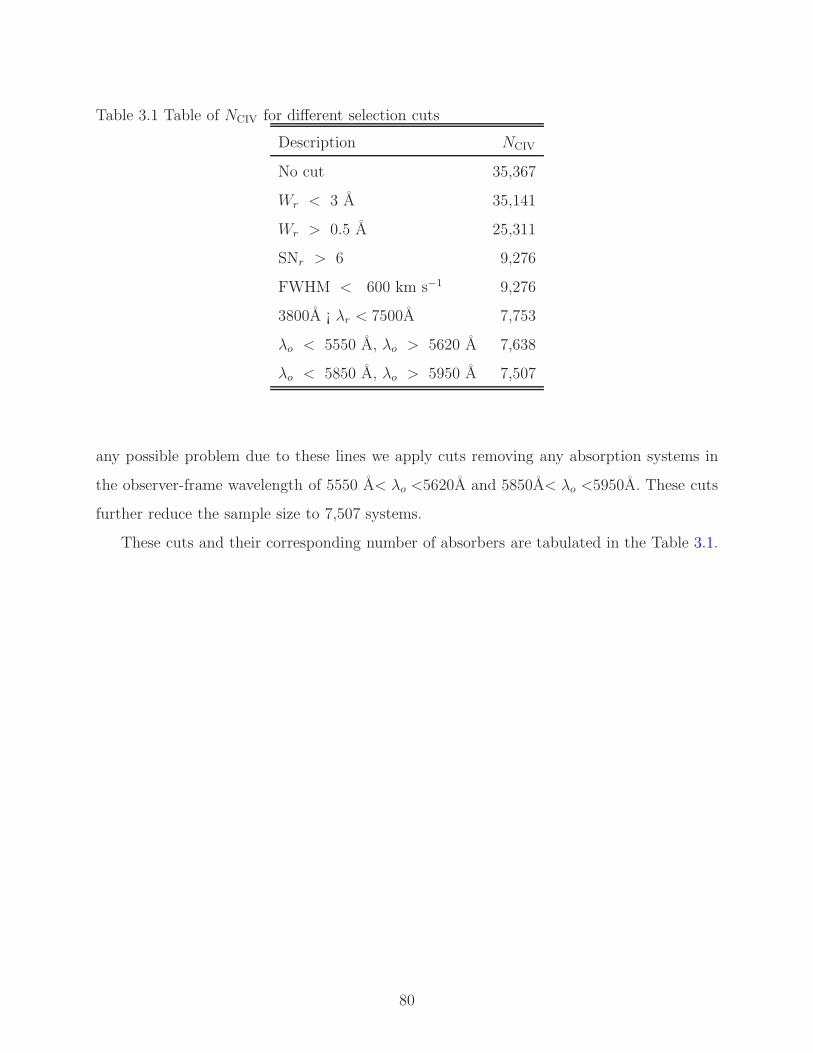
Table 3.1 Table of NCIV for different selection cuts
Description NCIV
No cut 35,367
Wr < 3 A 35,141
Wr > 0.5 A 25,311
SNr > 6 9,276
FWHM < 600 km s−1 9,276
3800A ¡ λr < 7500A 7,753
λo < 5550 A, λo > 5620 A 7,638
λo < 5850 A, λo > 5950 A 7,507
any possible problem due to these lines we apply cuts removing any absorption systems in
the observer-frame wavelength of 5550 A< λo <5620A and 5850A< λo <5950A. These cuts
further reduce the sample size to 7,507 systems.
These cuts and their corresponding number of absorbers are tabulated in the Table 3.1.
80
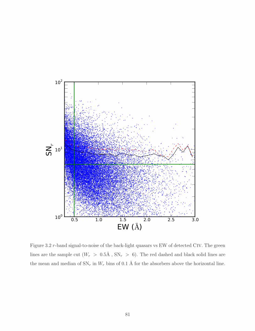
0.5 1.0 1.5 2.0 2.5 3.0
EW (!A)
100
101
102
SN
r
Figure 3.2 r-band signal-to-noise of the back-light quasars vs EW of detected CIV. The green
lines are the sample cut (Wr > 0.5A , SNr > 6). The red dashed and black solid lines are
the mean and median of SNr in Wr bins of 0.1 A for the absorbers above the horizontal line.
81

Figure 3.3 First and second of six example spectra.
82
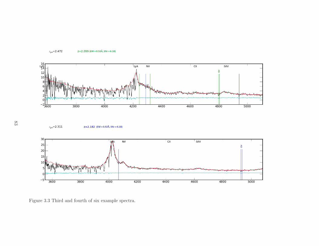
Figure 3.3 Third and fourth of six example spectra.
83

Figure 3.3 Example of six spectra out of thirty four weekest defined by signal-to-noise r-band between 6.0 and 6.15, and
equivalent-width are between 0.50 and 0.55. The C IV are evident in these spectra and suggest the sample to be complete. The
equivalent-width and signal-to-noise of r-band are also mentioned in the spectrum.
84
This analysis is done in the quasar rest frame. Because quasars at different redshift
contributed to different range of observable velocity space, I calculate the number of quasars
that contribute to any particular velocity range. Fig. 3.4 shows the number of quasars
contributing as a function of velocity from the quasar rest-frame. As can be seen from this
plot there are typically ∼12,300 quasars that contribute to the velocity range of interest.
3.5 ESTIMATION OF THE CROSS-CORRELATION FUNCTION
Using the halo model formalism described in section 3.3 we estimate the cross-correlation
function of quasars and C IV absorbers. Using the estimation given in Eq. 3.8. I used
the result from (Vikas et al. 2012, submitted to ApJ) of a large scale bias for quasars of
bqso = 3.71 and for C IV absorbers bCIV = 2.38 ± 0.62 at redshift 〈z〉 = 2.3. I use the large
scale bias estimation to determine the small scale bias. For this I have to assume, 〈N〉(M),
the functional form of average number of quasars and C IV absorbers in a halo of mass M .
For quasars I assume 〈N〉(M) to be of the form
〈N〉(M) =
0 for M < Mmin
1 Otherwise
(3.28)
The form of the above equation is motivated by the fact that the quasars are highly clustered
objects and hence are expected to live in large DM halos (Ross et al. 2009; White et al. 2012).
The time scale for SMBH merger is short (∼ 105 years) hence we do not expect more than
one quasar in a DM halo (Armitage and Natarajan 2002).
Now, using Eq. 3.19 I estimate Mmin such that at very small k (large scale) the bias
matches the scale independent bias. I perform a similar calculation for C IV absorbers with
a slightly different 〈N〉(M) functional form. For C IV absorbers I assume
〈N〉(M) =
0 for M < Mmin
MMmin
Otherwise
(3.29)
85

Figure 3.4 Number of quasars contributing at any given velocity in the rest-frame of quasar.
86

Table 3.2 Estimated parameters, using HOD formalism, for the Quasars and C IV absorbers
so that the linear bias is correct.
Quasars C IV absorbers
b 3.71 2.37
Mmin 2.61 × 10¹² 7.66 × 10¹⁰
The clustering of C IV absorbers is similar to galaxies (Vikas et al. 2012). Hence we may
expect many C IV absorbers to occupy a single DM halo. Hence the form of the above
equation does not limit the number of absorption systems in a halo.
We estimate the Mmin which matches the scale-independent bias for C IV absorbers.
Table 3.2 lists the estimated Mmin for both C IV absorbers and quasars. Fig. 3.5 shows the
bias as a function of minimum mass for both functional forms. We denote the minimum
mass and bias for C IV and quasars in the plot.
The power spectrum of the cross-correlation function from the two-halo term can be
written using Eq. 3.18. I get the cross-correlation function from the power spectrum using
an inverse Fourier transform.
ξ2hqso,CIV(r) =
1
2π2
∫
k3bqso(k)bCIV(k)P lin(k)sin(kr)
krd ln k (3.30)
The measurements of large-scale bias for quasars and C IV absorbers are estimated at
redshift z ∼ 2.3. Hence the cross-correlation function we estimated is only valid at about the
same redshift. Since our quasar sample for this study has a larger redshift range (1.5 < z <
3.8) we need to estimate the cross-correlation function at various redshifts. In the absence of
any knowledge of the rate of change of the large-scale bias with respect to redshift I assume
that the large-scale bias for quasars remains the same in our redshift range of interest. Thus
any change in the cross-correlation is governed by the change in the linear power spectrum
due to redshift.
Figure 3.6 shows the cross-correlation function of the two-halo term at redshifts z = 2.0
and 2.4. The cross-correlation function for z = 2.3 is calculated using the halo occupation
model formalism and that for at z = 2.0 is calculated from the values at z = 2.3 using the
redshift evolution of the linear power spectrum of dark matter.
87
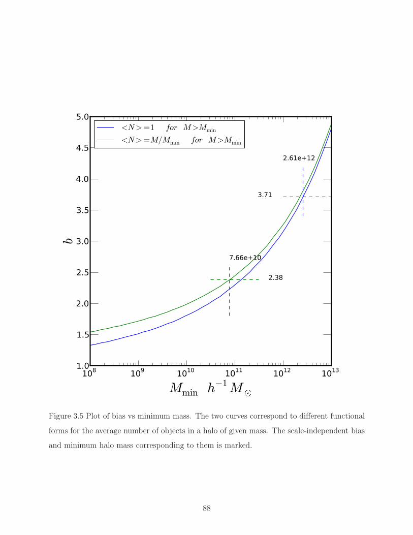
108 109 1010 1011 1012 1013
Mmin h"1M#1.0
1.5
2.0
2.5
3.0
3.5
4.0
4.5
5.0
b
2.38
7.66e+10
3.71
2.61e+12
<N>=1 for M>Mmin
<N>=M/Mmin for M>Mmin
Figure 3.5 Plot of bias vs minimum mass. The two curves correspond to different functional
forms for the average number of objects in a halo of given mass. The scale-independent bias
and minimum halo mass corresponding to them is marked.
88
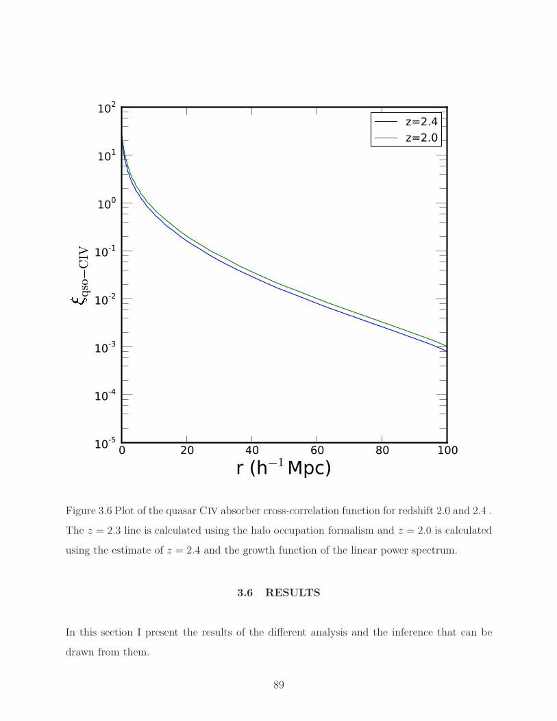
0 20 40 60 80 100
r (h$1Mpc)10-5
10-4
10-3
10-2
10-1
100
101
102
%qso&CIVz=2.4
z=2.0
Figure 3.6 Plot of the quasar CIV absorber cross-correlation function for redshift 2.0 and 2.4 .
The z = 2.3 line is calculated using the halo occupation formalism and z = 2.0 is calculated
using the estimate of z = 2.4 and the growth function of the linear power spectrum.
3.6 RESULTS
In this section I present the results of the different analysis and the inference that can be
drawn from them.
89

3.6.1 Estimation of parameters for the full dataset
I fit the model described by Eq. 3.10 to the observed BOSS data. I assume the redshift error
of BOSS quasars to be ∆zqso = 0.003(1 + zqso) (White et al. 2012). Figure 3.7 shows the
number density per unit velocity of the C IV absorbers as the blue circles. The error-bar on
the data is the Poisson error on the bin. The solid black line is the best fit model to the
data. The green region around the model line is the 1-σ error region of the model. The
error region is estimated by making 1000 realizations of the best fit covariance matrix and
calculating the 1-σ spread around every point. The best-fit parameters and their associated
errors are listed in Table 3.3.
Figure 3.8 shows the different components of the best-fit model. The solid line is the
one-halo component of the number density, Eq. 3.8, and the red region around the line is
the 1-σ error region. The dashed line is the two halo component of the number density,
Eq. 3.6 and the green region is the 1-σ error. The dotted line is the outflow component of
the number density, Eq. 3.9, and the blue region is 1-σ error region.
Figure 3.9 shows the correlation matrix at the best-fit value in parameter space. The
plot shows that there are some significant correlations between parameters of each models.
However, the lack of correlation between the outflow parameters (n2k, n4k, n6k) and non-
outflow parameters (n0σ0, ε, σβ, f) is evident. This suggest that our estimation of the
existence and overall strength of the outflow component is quite robust. There is also a lack
of corrleation between the one-halo parameters (f , σβ) and two-halo parameters (n0σ0, ε)
implying that our models are each independently constrained by the data.
3.6.2 Luminosity Dependence for Outflow
In this section I explore the dependence of the outflow on the luminosity of the quasars.
To explore this, I calculated the absolute magnitude of the backlighting quasars. I divide
the C IV absorbers into three bins (≈ 2500 absorbers each) according to tritiles of absolute
magnitude. Figure 3.10 shows the distribution of the absolute magnitude of the back-lighting
quasars of absorbers. The red-dashed lines show the tritiles of absolute magnitude of the
sample. For sub-samples I fit the model again fixing the non-outflow parameters (n0σ0, ε,
90

Figure 3.7 The model number density (solid line) and the observed number density (blue
circles) of the C IV absorbers as a function of velocity in the-rest frame of the quasar. The
error-bar on the data is estimated assuming Poisson distribution in the bins. The error
region for the model is derived by calculating the 1-σ error at every velocity point in 1000
realizations of the best-fit covariance matrix.
91

Figure 3.8 The individual components of the best-fit model. The one halo, two halo, and
outflow components are denoted by solid line, dashed line, and dotted line respectively with
red, green, and blue region as their 1-σ error region.
92

Figure 3.9 Correlation matrix of the best-fit model. The existence of many significant cor-
relations between parameters is evident. However, the lack of correlation between outflow
parameters (n2k, n4k, n6k) and non-outflow parameters (n0σ0, ε, σβ , f) is also clear, which
suggests the robustness of the outflow detection.
93

Table 3.3 The best-fit parameters of the model for all absorber data.
Parameter Best Fit
n0σ0 1.558 ± 0.188 × 10⁻³ Mpc−1
ε −2.884 ± 0.107
σβ 3.451 ± 1.925 × 10⁻⁴ km s−1
f 8.091 ± 4.519 × 10³
n2k 5.736 ± 0.613
n4k 1.373 ± 0.485
n6k 1.540 ± 0.304
σβ , f) to be same as the best-fit of the entire sample (shown in Table 3.3). I allowed the
outflow parameters (n2k, n4k, n6k) to vary and get the best-fit outflow parameters for each
sub-sample. Table 3.4 shows the best-fit outflow parameters for the high (low), medium
(medium), and low (high) absolute magnitude (luminosity) sample. Figure 3.11 shows the
best-fit outflow components for the low, medium and high absolute magnitude samples. The
red, green and blue line shows the outflow component for low, medium, and high luminosity
samples respectively. This plot gives strong evidence of the outflow being at higher velocity
for the brighter quasars compared to lower brightness one.
I also try to estimate if there is any dependence of the number of outflow systems on the
quasar luminosity. Table 3.5 lists the expected number of CIV systems for each component as
a percentage of the expected total. I calculate the expected number for each given component
by integrating the component for the whole range of β. It is evident that the abundance
of the outflow component for low, medium and high luminosity are consistently decreasing
with increasing luminosity. An inference can be drawn from these observations that the
luminosity tends to push absorption systems to higher velocity, while destroying a fraction
of absorbtion systems. Table 3.6 shows the number-density-weighted mean velocity of the
outflows for the three different samples and for all absorbers.
94

Table 3.4 The best-fit parameters of the model for all absorber data.
Parameter Mr < −27.09 −27.09 < Mr < −26.45 Mr > −26.45
n2k 3.188 ± 0.826 5.774 ± 0.978 7.459 ± 1.102
n4k 1.122 ± 0.712 0.651 ± 0.813 2.905 ± 0.948
n6k 1.693 ± 0.482 1.588 ± 0.520 0.840 ± 0.529
Table 3.5 Individual component as a percent of the total sample.
Sample One Halo Two Halo Outflow
Mr < −27.09 13.46 ± 0.50% 78.57 ± 0.05% 7.97 ± 0.15%
−27.09 < Mr < −26.45 13.20 ± 0.52% 77.47 ± 0.05% 9.33 ± 0.15%
Mr > −26.45 16.52 ± 0.64% 71.34 ± 0.05% 12.13 ± 0.16%
All 14.32 ± 0.57% 75.46 ± 0.05% 10.23 ± 0.09%
Table 3.6 The weighted mean velocity of the outflow.
Sample Velocity km s−1
Mr < −27.09 3786 ± 77
−27.09 < Mr < −26.45 3191 ± 63
Mr > −26.45 2902 ± 49
All 3232 ± 34
95

Figure 3.10 Distribution of the absolute magnitude of the back-lighting quasars of absorbers.
The red-dashed lines indicate the tritiles of the sample (-27.09,-26.45) mag.
96

Figure 3.11 Outflow component of the low, medium and high luminosity samples. The red,
green and blue lines are outflows from low, medium and higher luminosity sample and the
red, green and blue regions around them are the 1-σ errors of the outflows. The total number
of systems is smaller (higher) for brighter (dimmer) quasars.
97
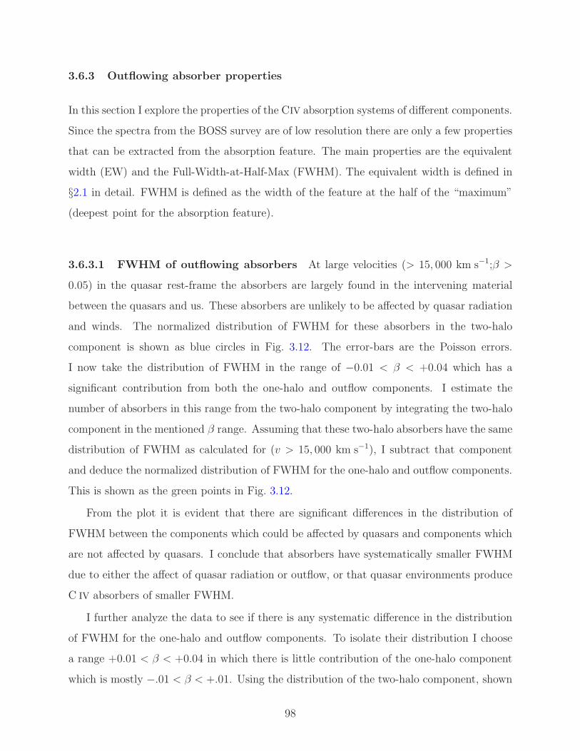
3.6.3 Outflowing absorber properties
In this section I explore the properties of the CIV absorption systems of different components.
Since the spectra from the BOSS survey are of low resolution there are only a few properties
that can be extracted from the absorption feature. The main properties are the equivalent
width (EW) and the Full-Width-at-Half-Max (FWHM). The equivalent width is defined in
§2.1 in detail. FWHM is defined as the width of the feature at the half of the “maximum”
(deepest point for the absorption feature).
3.6.3.1 FWHM of outflowing absorbers At large velocities (> 15, 000 km s−1;β >
0.05) in the quasar rest-frame the absorbers are largely found in the intervening material
between the quasars and us. These absorbers are unlikely to be affected by quasar radiation
and winds. The normalized distribution of FWHM for these absorbers in the two-halo
component is shown as blue circles in Fig. 3.12. The error-bars are the Poisson errors.
I now take the distribution of FWHM in the range of −0.01 < β < +0.04 which has a
significant contribution from both the one-halo and outflow components. I estimate the
number of absorbers in this range from the two-halo component by integrating the two-halo
component in the mentioned β range. Assuming that these two-halo absorbers have the same
distribution of FWHM as calculated for (v > 15, 000 km s−1), I subtract that component
and deduce the normalized distribution of FWHM for the one-halo and outflow components.
This is shown as the green points in Fig. 3.12.
From the plot it is evident that there are significant differences in the distribution of
FWHM between the components which could be affected by quasars and components which
are not affected by quasars. I conclude that absorbers have systematically smaller FWHM
due to either the affect of quasar radiation or outflow, or that quasar environments produce
C IV absorbers of smaller FWHM.
I further analyze the data to see if there is any systematic difference in the distribution
of FWHM for the one-halo and outflow components. To isolate their distribution I choose
a range +0.01 < β < +0.04 in which there is little contribution of the one-halo component
which is mostly −.01 < β < +.01. Using the distribution of the two-halo component, shown
98
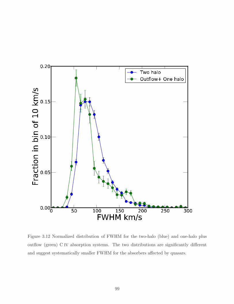
Figure 3.12 Normalized distribution of FWHM for the two-halo (blue) and one-halo plus
outflow (green) C IV absorption systems. The two distributions are significantly different
and suggest systematically smaller FWHM for the absorbers affected by quasars.
99

as the blue points in Fig. 3.13, I determine the normalized distribution for the outflow
component which is shown as green points in the figure. For the range −0.01 < β < +0.01
there is a significant contribution of the outflow as well as the two-halo terms. Assuming
the distribution of the other components, I determine the normalized distribution of the
one-halo component, which is shown as red points in the figure.
The FWHM distributions of outflow and one-halo absorbers in Figure 3.13 are quite
noisy. It is difficult to quantify the difference between the one-halo and outflow distributions.
However, the outflow component does shows an excess at lower FWHM. It can be inferred
that the outflow components have a systematically lower FWHM compared to both two-halo
and one-halo components. The estimate of the outflow and one-halo distributions are very
anti-correlated as they are isolated from the combined distribution. This anti-correlation
makes the differences, appear up to two times larger than they actually are. I used a
Kolmogorov–Smirnov (KS) test to test the significance of difference between the one-halo
and outflow components. The null hypothesis is that the distribution of one-halo and outflow
FWHMs are the same. I made 1000 realizations of the FWHM distribution by shuffling the
FWHM of the absorbers in the range −0.01 < β < +0.04. For each realization I estimated
the “ks-distance” between the one-halo and outflow distribution as the maximum difference
between the cumulative distribution of the two samples. The distribution of the ks-distance
is shown in Figure 3.14. The red dashed line shows the ks-distance of outflow and one-halo
distribution from Figure 3.13. It is evident that the significance of the difference is high
(p-value ∼0.001). The p-value value signifies the probabblity of getting the same result by
chance. I conclude that the FWHM of the absorbers in outflow is different compare to the
one in the host halo of the quasars.
3.6.3.2 Equivalent width of outflowing absorbers I follow a similar approach for
estimating the distribution of equivalent width as I did for FWHM in §3.6.3.1. Figure 3.15
shows the normalized distribution of equivalent width for the two-halo component in blue
points and the one-halo plus outflow in green. The two-halo component is derived from the
absorbers with velocity (> 15, 000 km s−1). The one-halo plus outflow component is derived
from −0.01 < β < +0.04, subtracting the two-halo component. It is evident from the
100
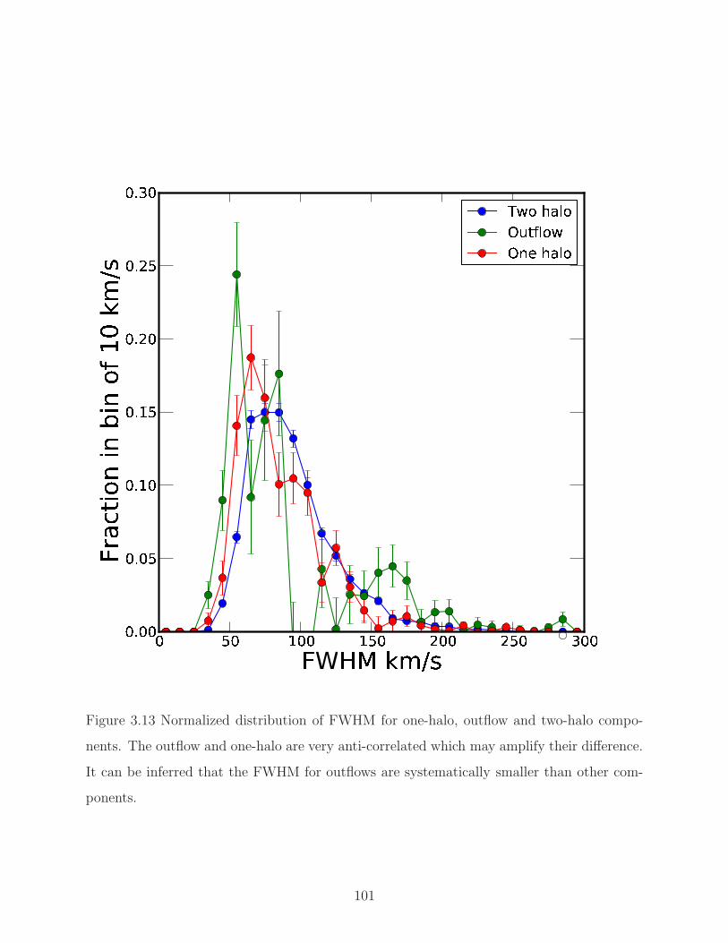
Figure 3.13 Normalized distribution of FWHM for one-halo, outflow and two-halo compo-
nents. The outflow and one-halo are very anti-correlated which may amplify their difference.
It can be inferred that the FWHM for outflows are systematically smaller than other com-
ponents.
101

Figure 3.14 The ks-distance of 1000 random realizations of the FWHM distributions of the
one-halo and outflow components.
102

distribution that the two-halo component is steeper compared to the one-halo plus outflow
and hence the absorbers in the quasar environment posses systematically larger equivalent
width compared to the two-halo term.
Following the steps of the §3.6.3.1, I further explore the difference between the out-
flow and one-halo components. I estimate the equivalent width distribution for the outflow
component from the absorbers in the range +0.01 < β < +0.04 subtracting the two-halo
component. I determine the distribution for the one-halo component from the absorbers in
the range −0.01 < β < +0.01 subtracting outflow and two-halo components. Figure 3.16
shows the equivalent width distribution of the two-halo, outflow and one-halo components
in blue, green and red respectively. There is no significant difference evident from this plot
due to the large error-bars and scatter.
3.6.4 Comparison with other result
There have been various previous studies of narrow C IV absorbers intrinsic to the quasars.
These studies try to model the observed number density using very simplistic models. The
model adopted in this study is a more physically accurate and statistically consistent way
to estimate the outflow component.
Wild et al. (2008) models the expected number density of absorbers by extrapolating the
best-fit power-law correlation function, determined in the distance range of 10-100 Mpc, to
small (kpc) scales. They find excess absorbers up to 150 Mpc away from the quasar. This,
unfortunately, result is not directly comparable to the results of this chapter as the they did
their analysis in comoving distance space and I choose velocity space of the quasar. The
result of their paper that excess of absorbers can not be explained by clustering alone holds
true for this study even after using more realistic handling of correlation function scaling to
smaller scale. The sample size of their C IV absorbers is 6,459 where as this study uses 7,507
absorbers, however, in this study we remove a large portion of spectrum to make cleaner
data.
Nestor et al. (2008) adopted a more detailed model for number density compared to
Wild et al. (2008). They modeled the number density of absorbers by adopting an intrinsic
103
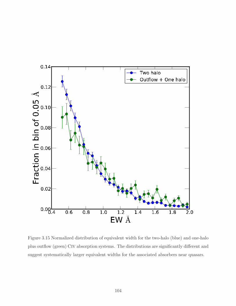
Figure 3.15 Normalized distribution of equivalent width for the two-halo (blue) and one-halo
plus outflow (green) CIV absorption systems. The distributions are significantly different and
suggest systematically larger equivalent widths for the associated absorbers near quasars.
104

Figure 3.16 Normalized distribution of equivalent width for one-halo, outflow and two-halo
components in blue, green and red respectively. No clear inference can be made from this
about the distribution of one-halo and outflow components.
105

term similar to the one-halo model in this chapter and constant term which is similar to two-
halo term of this chapter in the limit of large distances from the quasar. They constrained
their model from different parts of the velocity space and determined the outflow component
by subtracting the best-fit of the model from observed number density. My work improves
on this by modeling the two-halo term using halo occupation model formalism and taking
proper care of the redshifts of the quasars into account. Nestor et al. (2008) measured the
peak fractional contribution of the outflow to be ' 0.81 ± 0.13 at v ' 2, 000 km s−1. Their
results broadly match with the one from this chapter, but here I find the peak to be at
v ' 2, 100km s−1 contributing a smaller fraction (' 0.55 ± .05) of total absorbers. Their
result shows a tail of outflow velocity extending to v ' 12, 000 km s−1. Unlike theirs, I do
not find significant contribution of outflow at v > 8, 000 km s−1. I believe the difference
is due to simplistic model of Nestor et al. (2008) which does not consider the correlation
function. Due to the explicit modeling of the outflow component in my work, I believe, the
statistical inference of the outflow, is more robust and removes the tail of outflow at higher
velocity as they lack statistical significance. This study uses 7,507 C IV absorbers compared
to the 2,009 of Nestor et al. (2008). This large sample size enables better constrains of the
different components.
3.7 SUMMARY AND FUTURE DIRECTION
This study measures the velocity distribution and number density of the CIV absorbers in the
outflow of quasars using data from SDSS-III BOSS survey. I focused on the detailed modeling
of the number density of the absorbers according to their physical origin and undertook a
statistically robust measurement of different components. I conclude the following.
• The observed C IV absorbers can not be explained with the clustering of quasar and C IV
systems alone.
• The outflow system contribute ' 10% of the all C IV absorption systems detected.
• The outflow velocity peaks at ' 2, 100 km s−1 and are insignificant at > 8, 000km s−1.
• Brighter quasars have larger outflow velocities than dimmer ones.
106

• C IV absorbers affected by quasars have smaller full-width-half-max and larger equivalent
widths compared to the ones which are not affected by quasars.
A repeated analysis with the full BOSS sample will have ∼3 times more absorbers. The
statistical advantage of the full BOSS sample will greatly improve our ability to determine the
difference of properties (equivalent width, full-width-half-max) between outflowing absorbers
and clustering absorbers in the host halos of the absorbers.
107

4.0 SUPERNOVA IA COSMOLOGY AND SYSTEMATICS
Supernova Ia cosmology burst onto the center stage of cosmology when it was used to discov-
ering the acceleration of the expansion of the universe (Riess et al. 1998; Perlmutter et al.
1999). The next challenge, since the discovery of dark energy, has been to estimate its
equation of state, w, which describes the relation of its pressure to its energy density. The
generation of surveys that followed, such as ESSENCE, aimed to measure the w of dark
energy. In addition to estimating the value of w, it is important to measure the error on it
both statistical and systematical.
The new generation of supernova surveys like Pan-STARRS, DES, and LSST will yield a
much larger SN Ia sample. These large samples of SN Ia will measure w with greater precision
and will be instrumental in measuring the evolution of w over cosmic time. However, to reach
the full potential of these large samples of SN Ia data, which have the potential to give a much
smaller statistical error, we must improve our understanding of systematic errors, as they
do not decrease with large sample sizes. Therefore, a good estimation of systematic errors is
critical in order to provide a guide to channel the effort to tackle the largest systematic error
contributor. All recent SN Ia analysis suggest a high importance to estimating systematic
uncertainties (Conley et al. 2011; Kessler et al. 2009a; Wood-Vasey et al. 2007).
This chapter follows the trend of improving upon the estimation of systematics and
applying the improvements to the SN Ia data from the ESSENCE survey. In §4.1, I explain
how SN Ia are useful for understanding cosmology. I describe the effect of dust on supernova
cosmology in §4.2 and highlight the dependence of the dust uncertainty on the possible
progenitors. In §4.3, I describe the origin of the SN Ia data that is being used for the
study. I explain the method of fitting the light curves, which is essential to the estimation
of intrinsic parameters for the individual supernova, in §4.4. In §4.5, I explain the tool used
108

to generate the Monte Carlo simulations for the surveys and also explain the properties of
the simulation data generated by the tool. §4.6 presents the description of the systematic
errors that could be affecting the cosmological inference and the estimation of those errors
for our data. Finally, in the last section of this chapter, §4.7, I summarize the conclusions
from our study and present future direction for this study.
4.1 COSMOLOGY WITH SUPERNOVA IA
In classical physics, we can describe the distance, D, of a source with intrinsic luminosity,
L, and measured flux, F , as
D =
√
L
4πF(4.1)
Since the discovery of the acceleration of the expansion of the universe, requiring a
component of universe to have negative pressure, the standard way to describe dark energy
is by its equation of state, P = wρc2. Assuming Einstein’s general theory of relativity holds,
the “luminosity distance”, Dl, is given by
Dl =(1 + z) c
H0
∫ z
0
dz′√
Ωm (1 + z)3 + ΩΛ (1 + z)3(1+w)(4.2)
where Ωm and ΩΛ are the ratios of the densities of matter and dark energy to the critical
density of the universe. Here we have assumed the universe to be flat (ΩΛ = 1−Ωm). Using
the luminosity distance, we can write the distance modulus as follows
µ ≡ m − M = 5 log Dl − 5 (4.3)
where m is the apparent magnitude, which is a measure of flux, and M is the absolute
magnitude, which is a measure of luminosity, and Dl is luminosity distance in units of parsecs.
Standard candles have the same luminosity, making the absolute magnitude a constant for
all SN Ia observation. We can use Eq. 4.3 to constrain the cosmological parameters Ωm
and w if we have a sufficiently large number of supernovae Ia with well-measured apparent
magnitude and redshift.
109

As mentioned in §1.4.1, the supernova Ia’s “standardness” can be improved by using
the brighter-slower and brighter-bluer correlations. Using these correlations, Eq. 4.3 can be
modified as follows
µ ≡ m − (M − α shape + β color) (4.4)
where α and β are the global correlations of brightness-slowness and brightness-color, and
shape and color are parameters describing the slowness and color of the individual supernova
Ia light curves.
4.2 DUST EXTINCTION AND THE RELATIONSHIP BETWEEN DUST
AND SN IA PROGENITORS
One of the largest sources of uncertainty is the lack of understanding of dust in the host
galaxies of supernovae and their local environments. The estimation from the most studied
supernovae suggests steeper dependence of extinction versus wavelength with typical RV
values of ≈ 2 (Wang 2005; Krisciunas et al. 2007), compared to RV = 3.1 as observed for
the Milky Way galaxy (Schlegel et al. 1998).
The source of dust extinction can be divided into two components: 1) dust from the
host galaxy; 2) dust from the local environment of the progenitor. The dust due to the host
galaxy would not depend on the progenitor of the supernova, but the local environment dust
could be highly correlated with the type of progenitor. In the single degenerate model, the
progenitor accretes from a companion through Roche-lobe overflow and is likely to exhibit
a small explosion before the supernova (Nomoto 1982). Such small explosions or a series of
them can create dust clouds around the progenitor (Corradi 2003; Bujarrabal et al. 2010).
These progenitors also reside in star-forming regions of the galaxies, which are inherently
dusty environments. For these reasons, the single degenerate progenitors are expected to be
in environments with more dust extinction. In the case of the double degenerate progenitor,
the binary system is composed of two degenerate cores, meaning that star formation would
have ceased a long time before, so they are expected to be located in less dusty environments.
They would still, however, suffer from dust extinction due to the dust in the host galaxy.
110

The canonical value of RV in Milky Way is 3.1, but it ranges from 2-6 along different line
of sight (Schlegel et al. 1998). In a region of dense star formation, RV can be as small as
≈ 2 (Martin et al. 1989; Larson et al. 1996; Gordon and Clayton 1998; Larson et al. 2000;
Clayton et al. 2003; Gordon et al. 2003).
The treatment of host galaxy extinctions is very important for supernova cosmology.
IT is treated several different ways in the literature: 1) assume the AV to be linear with
flat prior (Perlmutter et al. 1999; Knop et al. 2003); 2) use models of the dust distribution
(Hatano et al. 1998; Commins 2004; Riello and Patat 2005) in galaxies to model line of sight
extinction values (Riess et al. 1998; Perlmutter et al. 1999; Tonry et al. 2003; Riess et al.
2004); 3) assume that the distribution of host galaxy AV is of exponential form (Jha et al.
2007); 4) use self-calibration within a set of low-z supernovae to obtain a color versus AV re-
lationship and assume the relation for the full set (Astier et al. 2006). Different assumptions
have different strength and weaknesses. The flat prior assumption assumes the least amount
of knowledge about the extinction, but it also allows the unphysical value of negative AV .
The method of modeling the dust distribution is physically motivated, but it relies on the
accuracy of our understanding of the complicated process of dust formation. The Jha et al.
(2007) derivation of the AV distribution assumes a particular distribution of color, and the
highly extincted objects often affect the fit of the overall dust law, even though they may
represent a separate population.
4.3 SUPERNOVA DATA FOR THIS STUDY
4.3.1 ESSENCE Supernova Survey
Designing surveys to look for supernova Ia is a difficult challenge because supernovae occur
only a few times per millennium in a typical galaxy, which makes, concentrating on a few
galaxies inefficient. Supernovae are transient events that last for only a couple of months.
A possible observation strategy could be taking images of large part of the sky regularly, so
that a new bright spot in the image could be identified. This strategy would give candidates
111

for supernova Ia that would need to be watched more carefully in order to be identified as
real SN Ia.
Equation of State: SupErNovae trace Cosmic Expansion Survey (ESSENCE) was a
ground-based multi-year project aimed to identify the supernova Ia in the redshift range of
0.2 < z ≤ 0.8. The survey was conducted using the Blanco 4m telescope at Cerro Tololo
Inter-American Observatory (CTIO) located in Chile. It used passbands with a MOSAIC
wide-field CCD camera. The survey took repeated images in R and I passbands with a
cadence of a few days separation for three consecutive months each year. The base bands, R
and I, were chosen to coincide, at a redshift of z ∼ 0.5, with the rest frame bands, B and V,
where our understanding of SN Ia is best. When the survey identified a potential supernova
Ia, several different large aperture telescopes (Keck, VLT, Magellan, Gemini) followed up on
the object. Taking spectra from large telescopes helped to identify the type of supernova
and also gave accurate measurements of the redshift of the supernova.
The goal of the survey is to put tight constraints on the equation of state of dark energy,
w. The ESSENCE survey was designed to take advantage of the uniformity of photometry
because it used a single telescope and instrument throughout the survey period. The survey
also focused on the sources of systematic errors that are now a bigger source of uncertainty
than the statistical error associated with the small number of supernova Ia observations. The
survey collected data for 197 half nights over a six year period of observation. The survey
confirmed 203 supernova Ia during the entire observation period. The detail of the design of
the ESSENCE survey is elaborated in Miknaitis et al. (2007).
Wood-Vasey et al. (2007) have done the cosmological analysis using three years of data
from ESSENCE. They explore, in great detail, the systematic error for the analysis and
their estimation. Table 5 in that paper, lists all the individual systematics considered and
estimations of the effect on w.
4.3.2 Low redshift sample
To a large extent our understanding about SN Ia comes from the well-observed sample of
low redshift,. They have been observed at densely sampled epochs in multiple pass-bands.
112
Understanding the low redshift sample enables us to produce light curves for the high redshift
SN Ia, correcting for extinction and incorporating the brightness-color and brightness-shape
correlations. The low redshift sample comes from various sources including the: Calan/Tololo
survey (Hamuy et al. 1996), CfAI(Riess et al. 1999), CfAII (Jha et al. 2006). The sources are
compiled in Jha et al. (2007) with much emphasis on making the measurements as accurate
as possible. I use this sample of 125 nearby SN Ia for our study. In addition to light curve
measurements, the low redshift sample is also very important for cosmological analysis, as
our goal in this study is to obtain the tightest constraint on w. The absolute distances of
the supernovae depend on the parameter w and the Hubble parameter h. However, since the
ratio of the distances of high-redshift supernovae to low-redshift supernovae is independent
of the Hubble parameter h, hence the low-redshift supernovae sample enables us to make
more robust constraints on w, by not being dependent on absolute knowledge of h and the
luminosity of SN Ia.
4.3.3 Other Surveys
SN Ia surveys yield a limited number of events during the survey lifetimes. Using events
from different surveys from analysis is an easy way to improve the sample size. In addition to
having better statistics, using various surveys has the benefit of sampling different redshift
ranges, which will produce better constraints on the cosmological parameter. In this study,
we includes data from SDSS (Kessler et al. 2009a, 115 SN Ia), SNLS (Astier et al. 2006, 65
SN Ia), and HST (Riess et al. 2007, 20 SN Ia).
4.4 LIGHT CURVE ESTIMATOR
SN Ia exhibit variability in light curve shape, colors, intrinsic luminosity, and spectral fea-
tures. These properties are measured in the observer reference frame using photometry at
non-periodic intervals using various filters. The redshifting of the spectra makes different
parts of rest-frame spectra available for measurement. Apart from intrinsic variability of the
113

SN Ia spectrum, the difference in dust absorption along different lines of sight affects the
observed properties of SN Ia. Converting observed properties of SN Ia to the rest-frame prop-
erties of interest is a non-trivial task but of central importance to analysis. Many such light
curve estimators have been developed, e.g. MLCS2k2 (Jha et al. 2007), SALT II (Guy et al.
2007), BayeSN Mandel et al. (2011). In this study, we are using the SALT II light curve
estimator.
4.4.1 SALT II
SALT II models the mean evolution of the spectral energy distribution sequence of super-
novae Ia and the variation with a few dominant components. It also allows a time indepen-
dent variation with color. The following functional form of flux, F , is assumed:
F (SN, p, λ) = xo [Mo(p, λ) + x1M1(p, λ) + ...] exp [c CL(λ)] (4.5)
where p is time in the rest-frame since the date of maximum luminosity in B-band, and λ
is the rest-frame wavelength of the supernova. Mo(p, λ) is the average spectral sequence;
Mk(p, λ), for k > 0, represents additional components that describe the main variability
of supernova Ia; CL(λ) represents the average color correction law; and c is defined as
(B − V )max− < B − V >. Therefore, xk and c are individual supernova Ia parameters and
Mk is a global parameter.
SALT II uses multi-band light curves to train the model. It also uses the spectroscopic
data to improve the model resolution in wavelength space. Use of spectroscopic information
enables the K-correction to be treated in a consistent manner.
The above model is constructed using the nearby supernova Ia sample and the high red-
shift supernovae from the Supernova Legacy Survey (Astier et al. 2006; Conley et al. 2011).
Including the high redshift supernova Ia enables us to constrain the model in the wavelength
range of the U-band, which can not be done using only nearby supernovae Ia because they
have poor U-band data due to the opacity of Earth’s atmosphere in the ultraviolet. Us-
ing these datasets the model from Eq. 4.5, is constrained at grid points in phase, p, and
wavelength.
114

Once the training of the model is completed, SALT II can be used to evaluate the light
curve of any supernova Ia by trying to evaluate the best fit for variability parameters xk and
c. The model should, therefore, be able to produce the light curve for any supernova Ia.
Using the parameters of SALT II, Eq. 4.4 would be written as
µ ≡ m − M + α x1 − β c (4.6)
4.5 MONTE CARLO SIMULATION
Systematic studies on combined SN Ia samples can be done, in principle, by selecting subsets
of whole datasets, according to different properties, and doing complete analysis on the
different subsets. However, this would require a vary large dataset so meaningful constraints
on the subset could be found. The current worldwide SN Ia sample is far from reaching the
required size (>10,000) for such analysis, but the problem can be overcome if we are able
to create a simulated dataset that takes into account the effect of different parameters on
the dataset. Although simulated data is not useful for finding new systematics in the data,
it can accurately measure the existing systematic errors for any parameter modeled in the
simulated dataset.
4.5.1 SNANA
SNANA is a publicly available simulation tool designed to model SN Ia datasets. The soft-
ware is described in Kessler et al. (2009b). The software contains a Monte Carlo simulator,
a light curve fitter, and a cosmology fitter. The software is designed to use multiple SN Ia
light curve models and can be easily extended to include new models of light curve fitting.
SNANA provides the ability to specify the description of any survey, such as the MJD
of survey observations, filters, and many other properties, which enables the Monte Carlo
simulator to generate supernova datasets closely following the real data properties. SNANA
also provides a way to specify the desired properties and the model used for light curve fitting.
These properties include, but are not limited to, specifying the brightness-shape correlation,
115

brightness-color correlation, dust extinction distribution and various other model parameter
distributions that could affect the distribution of the supernova Ia data. The software also
has the capability to specify a quality cut on the supernova data before it is accepted as a
reliable supernova observation. To model an individual survey, we can use the specific filters
and the quality based on the filters and actual observational conditions.
The SNANA software provides several light curve fitter options, including SALT II and
MLCS2k2, and provides an easy way to support new light curve models. These options help
to achieve some uniformity in the light curve model, makeing it easy to test the robustness of
the analysis. The light curve fitter provides various methods to obtain the best fit value of the
parameters and produces the measurements of different parameters of individual supernova.
The software also provides a cosmology fitter that takes the output of the light curve
fitting and attempts to fit the global parameters, which could be the cosmological parameter
or the global brightness-shape or brightness-color correlation. All of these parameters are
provided in the simulation step, so we can check if there is a bias introduced by the analysis.
There are many other capabilities of the SNANA tool, but I have only outlined those
that are used by our analysis.
4.5.2 Simulation data
I created the simulation dataset to closely follow the characteristics and composition of the
real dataset, so the simulated data is an accurate representation of the real dataset. I used
the SNANA software described in section 4.5.1 to make one hundred realizations of the
dataset. The real dataset consists of a collection of surveys. To imitate the real data, I
generated simulated data for the LOWZ, SDSS, ESSENCE, SNLS, and HST surveys, having
125, 115, 150, 65, and 20 supernovae respectively. I used custom survey definition files to
generate appropriate datasets for each survey and then added the simulated data to make
the complete simulated dataset used for analysis. I generated all the simulated data using
the SALT II model. After the SN Ia data was generated, I concatenated the data from
different surveys to make the complete dataset representing the real data. I used the light
curve fitter on the simulated dataset to measure the properties of the individual light curves.
116

I then used the cosmological fitter to get the best fit cosmological parameters, assuming a
flat universe.
4.6 SYSTEMATIC UNCERTAINTIES OF THE SUPERNOVA ANALYSIS
In this section, I aim to estimate the errors due to the systematics that affect this analysis.
I first make a list of possible systematic error sources and then predict how they could be
affecting our data in section 4.6.1. In section 4.6.2, I describe the methodology I used to
find the probability distribution of the error introduced by any specific systematic error. In
section 4.6.3, I describe the analysis of the systematic error for our data sample using the
methodology described in section 4.6.2.
4.6.1 List of systematic uncertainties
In this section, I mention and explain various systematic errors that could affect the inference
of cosmological parameters.
1. Dust and Milky Way Extinction: Supernovae Ia are important to cosmology be-
cause they are standard candles. However, their observed brightness can be affected by
material, such as dust, that lies between the supernova and us. While the intergalactic
medium is quite thin and does not contain much dust that would affect the brightness,
our own Milky Way galaxy contains a significant amount of dust. The host galaxies of
supernovae can also contain a significant amount of dust. Our ability to determine the
absolute brightness relies on our ability to correctly estimate the dimming of brightness
due to dust. Dust extinction affects smaller wavelengths more than larger wavelengths,
so the net affect of dust extinction is to make the supernova appear redder. The avail-
ability of multi-band photometry data enables us to determine the color of high redshift
supernova. Each supernova may be expected to have a different dust extinction, due to
environment effects, however, it is not possible to correct for the effect of dust extinction
using only color information. Estimation of the global distribution of dust extinction
117

is used to correct the individual supernova color. The well-observed nearby sample of
supernovae provides the distribution of supernovae in color space. Assuming the distri-
bution of the nearby sample to be true at higher redshifts, we can estimate the global
extinction distribution of the supernova sample. Any error in estimating the global dust
extinction affects the estimation of all supernova colors individually. The inference of
cosmological parameters is affected systematically.
2. Evolution of Dust Extinction: The extinction of supernovae Ia due to dust in the
host galaxies is not very well understood. There are reasons to think that there could
be evolution of dust in the host galaxies of supernovae Ia (Totani and Kobayashi 1999;
Jain and Ralston 2006), as the galaxies evolve with redshift affecting the dust content
due to various factors (e.g., star-formation, metalicity). Our measurement of dust ex-
tinction is not accurate enough to measure the redshift evolution of dust extinction. The
assumption of no evolution in dust extinction can lead to a systematic error dependent
on redshift.
3. Photometric Zeropoint: In astronomy, the prevalent way of measuring the flux is
using the magnitude system. The magnitude is defined as
m = −2.5 log(F ) + zeropoint (4.7)
where F is flux in unit of ergs per second per cm2 per Hz. The zeropoint and m have
the same unit of “mag”. Since every telescope and instrument has unique characteristic
behaviors, the zeropoint offset has to be calculated for each telescope, instrument, and
filter. Any systematic error in estimating the zeropoint for each filter will affect the mag-
nitude estimation for that pass-band data for all observations. These errors in zeropoint
offsets affect the supernova Ia data in following ways:
I) Cosmological analysis of supernovae Ia depends heavily on observations of low red-
shift supernovae Ia. As explained in section 4.4.1, the local supernova Ia are used
to train the light curve fitter and the result is used to estimate the light curve
for high redshift supernova Ia. These samples of local supernova Ia were observed
from multiple telescopes, using different instruments and various filters. The error
in photometric calibration would introduce systematic errors in training the light
118

curve fitter and thus would affect the determined properties (i.e., stretch, color) of
all the supernova Ia.
II) For the high redshift supernova survey (e.g., ESSENCE), a precise zeropoint esti-
mation for each different filter is also very important. Since the errors in zeropoint
offset for different filters are independent of one another, the errors could potentially
cause large errors in color. This color error will affect all the supernova Ia from
the survey. From Eq. 4.5, we can see that the color term is important to the train-
ing process and, in conjunction with color correction law, will systematically cause
under- or over-estimation of the extinction, affecting the estimation of cosmological
parameters.
4. Local flow: Supernova cosmology studies compare the low-redshift supernovae with a
high-redshift sample. The goal is to deduce the expansion history of the universe at
different redshifts. An implicit assumption used in this analysis is that the observed
supernova redshift is only due to the expansion of the universe. Because the redshift
measures the recession velocity, which is due to Hubble flow as well as peculiar velocity
of supernova in their local environment, the assumption is not strictly true. However, for
supernovae separated by large cosmological distances, the peculiar velocity cancels out,
as the directions are randomly distributed and do not induce bias in the measurements.
The low-redshift supernovae are not separated by large cosmological distances, so the
peculiar velocities could be correlated, and the net affect of having many supernovae
could be a nonzero peculiar velocity in the direction of the coherent motion of the local
universe. Such a residual will induce systematic error in the estimated expansion history
and will lead to incorrect inference of cosmological parameters. We currently do not have
precise information about the local flow, so to avoid introducing error due to local flow,
we need to remove some very nearby supernova from the sample.
5. Malmquist Bias: The Malmquist bias is the selection bias in a magnitude limited
survey where we selectively intrinsically brighter objects at large distance. As a result,
the properties of that sample that correlate with intrinsic brightness would also correlate
with redshift, even if there is no intrinsic evolution of that property with redshift. This
selection effect is enhanced because spectroscopic criteria are generally more stringent;
119

a faint supernova Ia may be too faint to take a clean spectra. This selection effect can
interfere with cosmological analysis in a few possible ways. Error in the measurement
of the strength of the shape-luminosity correlation is one possibility. For a given shape
of supernovae Ia, the selection effect would tend to choose the brighter supernovae Ia,
increasing the inferred shape-luminosity correlation. This mis-estimation will affect all
the supernova Ia in the sample.
Another way the Malmquist bias could affect the cosmological inference is by inducing
errors in the dust extinction of the supernova Ia. For any given intrinsic brightness of
supernova Ia, the selection effect will remove the supernova Ia with more dust extinction
and affect our estimation of dust extinction in the sample. The mis-estimation would
not be so bad, as it will be a true representation of the sample; however, selection effects
introduce a redshift dependence and produce a relative systematic error in high redshift
supernova Ia.
6. Rest Frame U/u Band: The rest frame U-band data for nearby supernovae Ia are
almost the same as the observer frame U-band data. Since the Earth’s atmosphere is not
completely transparent for U-band wavelength, our U-band data for nearby supernovae
is of poor quality and difficult to calibrate. For high redshift supernovae Ia the rest
frame U-band is redshifted to optical range, so they are well observed. Compared to
rest frame U-band observation of high redshift supernovae Ia, the nearby sample has a
big offset due to unreliable U-band data. Since training the light curve fitter is largely
dependent on the nearby supernovae Ia observations, the problematic U-band data can
inflict systematic errors on the light curve estimation of all supernovae Ia, which affects
the cosmological parameter estimation. The U-band measurements also exhibit a larger
dispersion and are inherently less standardizable, compared to other bands.
7. Intrinsic Brightness Evolution: Supernovae Ia are standardizable candles within
some accuracy. However, the possibility exists that supernovae Ia brightness evolves
with redshift. The studies looking to find such evidence have not able to find any, but a
weak evolution of brightness, at the level of a few percent, can not be ruled out. Such
error will place a redshift dependent error on the distance modulus of the supernovae Ia
and will systematically bias the cosmological parameter estimated from the analysis.
120

4.6.2 Methodology
In this section, I describe the generic methodology I have used to estimate the systematic
errors. I describe use the SNANA monte carlo simulation tool, described in section 4.5.1, to
model the systematic errors. For any given cosmological parameter X(p1, p2, ..., pn) where
pk is kth systematic parameter, the systematic errors on X can be written as
δX2sys =
∑
k
(
∂X
∂pk
)2
δp2k (4.8)
I assume here that the different parameters are not correlated with each other and can
be estimated independently. To estimate ∂X∂pi
, I generate a random realization of our final
supernovae Ia data from various surveys using SNANA and using pi = pi,True. I complete
the analysis of this dataset by using a light curve fitter and a cosmological fitter, using the
same parameter as in the simulation, and get the best fit value for X to be xi,True. I redo
the above analysis now assuming that I have mis-estimated parameter pi to be pi,True+∆ and
get the cosmological parameter X to be xi,True+∆. Using the above information, I can write
∂X
∂pi
(pi = pi,True) 'xi,True+∆ − xi,True
∆(4.9)
The estimation of ∂X∂pi
is only for one random realization. Our dataset sample is only one
realization of an infinite number of possible outcomes for any give set of parameters. To
completely characterize ∂X∂pi
, I need to find the probability distribution function of ∂X∂pi
. To
do so, I repeat the process, with different seed values, 100 times for any given parameter
analysis. The distribution ∂X∂pi
is then converted to a probability distribution function using
kernel density estimation. The estimated error on the cosmological parameter X due to
systematic pi can be written as
δX2sys,i =
(⟨
∂X
∂pi
⟩)2
δp2i (4.10)
121
4.6.3 Analysis
In this section, I present the results of the analysis of some of the systematic errors discussed
in §4.6.1. As mentioned in section 4.3.1, the main goal of the ESSENCE survey is to constrain
the dark energy equation-of-state parameter. I consider here the systematic error analysis,
one systematic at a time.
1. Dust and Milky Way Extinction: I estimate here the systematic error due to mis-
estimation of the dust extinction parameter β for SALT II (see Eq. 4.6). The current
estimated value of β for the nearby sample is ≈ 2.6 (Hicken et al. 2009; Kessler et al.
2009a). I estimate 〈∂w∂β〉 by following the process outlined in section 4.6.2. I first generate
a simulation of our dataset using SNANA with βsim = 2.6 . Using the simulated survey
dataset, I use the SALT II light curve fitter to estimate the light curve. I then fit for the
cosmological parameters by fixing the extinction parameter β to βsim + ∆β, βsim, βsim −∆β, where I choose ∆β to be 0.2 . Using the estimated w, I calculate the change in
estimation of w, ∆w, for the change of ∆β, which leads to an estimation of ∂w/∂β. I
also calculate the change in the estimated Ωm as indicated by ∆Ωm. To estimate ∂w/∂β
across the relevant range of β, I repeat this process for simulations with β = 1.6, 3.6. To
estimate 〈∂w/∂β〉 from ∂w/∂β, I repeat the process outlined above 100 times, in order
to estimate the probability distribution function of ∂w/∂β.
Figure 4.1 shows the ∆w and ∆Ωm for simulations of β = 1.6, 2.6, 3.6 . The distribu-
tion of points aligned on negatively sloped straight line indicates the line of degeneracy
in the w and Ωm plane, as a more negative value of w would tend to accelerate the expan-
sion of the universe while a more positive value of Ωm would decelerate the expansion(for
a flat universe). The subplots show the difference in distribution for ∆w and ∆Ωm for
different β. The plot explains the need to estimate ∂w/∂β at three different β values
in order to be representative of the full range of β. A closer look at the plot reveals
that for the lower extinction simulation, the distribution of ∆w peaks closer to near zero
compared to the higher extinction simulations. This confirms that smaller extinction
data suffer less systematic extinction error due to mis-estimation of β.
122
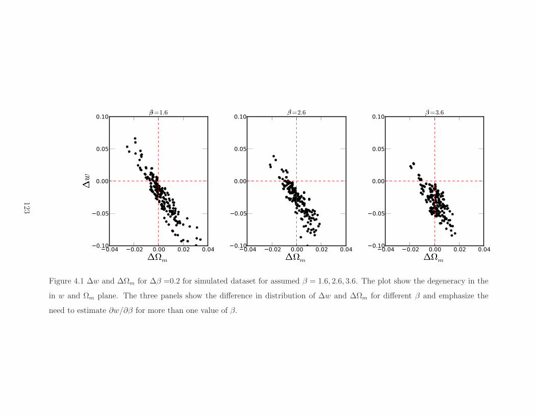
'0.04 '0.02 0.00 0.02 0.04( )
m
'0.10
'0.050.00
0.05
0.10
*w
+
=1.6
'0.04 '0.02 0.00 0.02 0.04( )m
'0.10'0.050.00
0.05
0.10
+
=2.6
'0.04 '0.02 0.00 0.02 0.04( )
m
'0.10'0.050.00
0.05
0.10
+=3.6
Figure 4.1 ∆w and ∆Ωm for ∆β =0.2 for simulated dataset for assumed β = 1.6, 2.6, 3.6. The plot show the degeneracy in the
in w and Ωm plane. The three panels show the difference in distribution of ∆w and ∆Ωm for different β and emphasize the
need to estimate ∂w/∂β for more than one value of β.
123

Figure 4.2 shows the probability distribution function for ∂w/∂β estimated from the
100 different ∂w/∂β estimations. The distribution is estimated using a kernel density
estimator. The method involves convolving a Gaussian function with the histogram of
measurement to get a continuous and smooth probability density function.
Using the distribution, I estimate 〈∂w∂β〉 = −0.132. There have been a few studies of
dust extinction that estimated the error on the dust extinction parameter for SALT II.
Kessler et al. (2009a) find σRV= 0.5. Here I conservatively assume the error estimation
of σβ = 1.0 to be on conservative side. I calculate the systematic error due to dust
extinction to be
δw =
√
(⟨
∂w
∂β
⟩)2
δβ = 0.13
The most recent systematic error study from Conley et al. (2011) estimated the sys-
tematic error on w due to dust extinction to be σw ∼ 0.01. Due to the difference in
analysis the errors are not exactly comparable. However, I believe the difference is due
to our liberal assumption of error on the dust extinction and due to Conley et al. (2011)
having cleaner data with more passbands and excluding highly reddened SN Ia.
2. Photometric Zeropoint: Here I try to demonstrate and quantify the systematic error
due to zeropoint offsets for the ESSENCE data. ESSENCE data are taken in two pass-
bands, R and I. As mentioned in section 4.6.1, the zeropoint estimate for each band is
independent of the other. The systematic error then involves two parameters. I do the
joint analysis of these two parameters. I explore the zeropoint estimate error in the range
of [-.1,.1] in 11 bins for both the R and I bands. For each bin I generate 100 realizations
of data and complete the cosmological analysis. Figure 4.3 shows the equation of state
parameter w for an induced zeropoint offset in R and I band. The horizontal axis shows
the offset in the R band and the vertical axis shows the offset in the I band. The color
in any bin represents the derived value of w. The color-bar shows the mapping between
the value of w and color. This plot shows the amount of systematic error in w due to
zeropoints offsets. It also shows that if both bands suffer from the same error, then they
cancel each other when estimating color and produce the correct w.
Figure 4.4a and 4.4b show the probability distribution function for ∂w∂∆R or ∆I
for
the shift of 0.02 mag. The probability distribution is estimated using a kernel density
124

,0.8 ,0.6 ,0.4 ,0.2 0.0 0.2 0.4 0.6-w-.0.0
0.5
1.0
1.5
2.0
2.5
3.0
3.5
p(
/w/0)12w234=50.132
Figure 4.2 Shows the probability distribution function of ∂w/∂β estimated from 100 simu-
lation to estimate ∂w/∂β. I estimate 〈∂w∂β〉 from this distribution.
125

60.10 60.05 0.00 0.05 0.107R60.1060.050.00
0.05
0.10
8I
61.461.361.261.161.060.960.860.760.6
Figure 4.3 Shows the estimated value of w for zeropoint offsets in the R and I bands. The
degeneracy in the diagonal direction is due to the fact that the errors on the R and I bands
cancel each other (with a slope of 2) to give an accurate color estimation.
126

estimator. Using the probability distribution, I estimate the values of 〈 ∂w∂∆R
〉 = 1.811 and
〈 ∂w∂∆I
〉 = −3.487. The anti-correlation of the R and I band errors are expected because
estimation of supernova color depends on the rest-frame B-V color. The color is derived
from the K-correction of R and I band and effectively subtract the zeropoint error of
R and I. Using a known zeropoint offset error of 0.02 for both bands, I estimate the
systematic error on w to be
δw =
√
(⟨
∂w
∂∆R
⟩)2
δ∆R = 0.04
δw =
√
(⟨
∂w
∂∆I
⟩)2
δ∆I = 0.07
127

914 912 910 98 96 94 92 0 2 4:
w/
: ;I
0.00
0.05
0.10
0.15
0.20
0.25
0.30
p(
<w/ <=I)
> ?
w? @
I
A
=-3.487
(a) Probability distribution function of ∂w/∂Ishift.
B4 B2 0 2 4 6 8 10 12C
w/
C D
R
0.0
0.1
0.2
0.3
0.4
0.5
p(
Ew/ EF R)
G HwH IR
J=1.811
(b) Probability distribution function of ∂w/∂Rshift.
Figure 4.4 Shows the probability distribution function of ∂w/∂Ishift and ∂w/∂Rshift estimated from 100 simulated datasets. I
estimate < ∂w/∂Ishift >= −3.49 and < ∂w/∂Rshift >= 1.811 .
128

3. Local flow: As explained in section 4.6.3, the systematic error due to the local flow of
galaxies can be estimated from the real data by applying a minimum redshift cut (zmin).
I do the light curve and cosmological fitting for the data after applying the zmin on the
sample. Kessler et al. (2009b) found the w changes rapidly at z ∼ 0.015 and opted for
zmin = 0.02. Other authors estimated different values for zmin; for example, Conley et al.
(2007) found no significant effect of local flow and Riess et al. (2007) used zmin = 0.023.
The blue circles in the lower panel of figure 4.5 show the change in the estimation of
w, compared to w in the last bin of zmin = 0.029. The difference ∆w is clearly visible,
however compared to the error of w, the change is insignificant. I also compare our result
with the result from the SDSS supernova study of Kessler et al. (2009b). Since there are
many differences between this study and Kessler et al. (2009b), I explored whether the
difference is due to the different datasets or different analysis. I made a new dataset
that closely resembles the one from Kessler et al. (2009b) and repeated the analysis on
the new dataset. This reproduced the behavior of Kessler et al. (2009b), as shown in
the lower panel of figure 4.5. Because I was able to successfully reproduce the result, I
conclude that the difference in the result is due to data only and the method of analysis is
consistent. The upper panel of figure 4.5 shows the number of SN Ia in the corresponding
bins. As can be seen from this plot, the number of SN Ia in these bins is much higher
in our study. From the figure, I conclude that the local flow does not affect our result
systematically.
To make a better comparison, I simulated one hundred datasets emulating our
dataset. I compared how much the result from the simulation varies if we have ar-
tificial zmin. Figure 4.6 shows the hundred test simulations in gray, and the red line
indicates the one sigma range for those zmin bins. We see that ∆w varies in the range of
-0.1 to +0.1, which is completely consistent with the error on w from our dataset. This
gives further conformation that the local flow does not add any appreciable systematic
error to the cosmological parameter estimation.
129

0.012 0.014 0.016 0.018 0.020 0.022 0.024 0.026 0.028 0.030zmin
K0.4
K0.2
0.0
0.2
0.4
Lw
All Data
K09
0
5
10
15
20
25
# in b
in
Figure 4.5 The lower panel shows the change in w compared to the choice for last bin of
zmin = 0.029. The blue circles are our dataset. The red square is the reproduction of the
Kessler et al. (2009b) plot using a subset of all data that is common to their dataset. The
error bars denote the error on the estimation of w. The correct reproduction of low estimate
of w at zmin < 0.018 shows that the difference between these studies is purely data driven.
The upper panel gives the number of SN Ia in each bin. The larger number of supernova
in our studies (blue line compared to red one) removes the data sensitivity to local flow
systematics.
130
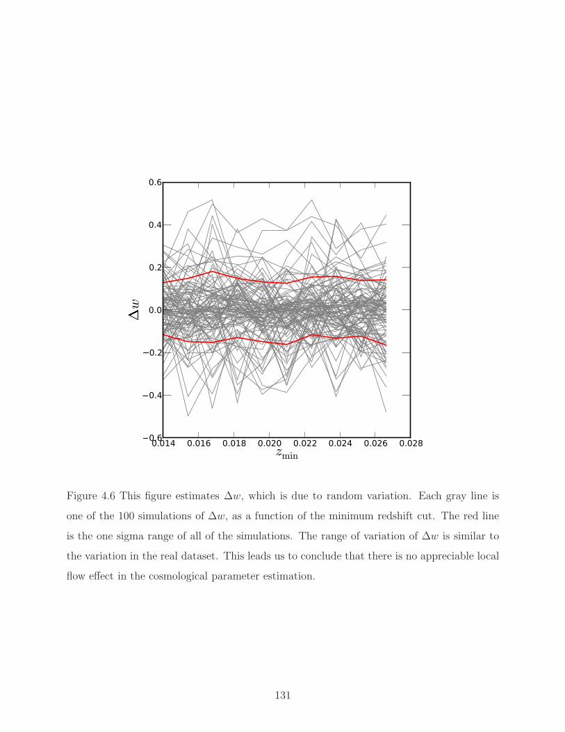
0.014 0.016 0.018 0.020 0.022 0.024 0.026 0.028zmin
M0.6M0.4M0.20.0
0.2
0.4
0.6
Nw
Figure 4.6 This figure estimates ∆w, which is due to random variation. Each gray line is
one of the 100 simulations of ∆w, as a function of the minimum redshift cut. The red line
is the one sigma range of all of the simulations. The range of variation of ∆w is similar to
the variation in the real dataset. This leads us to conclude that there is no appreciable local
flow effect in the cosmological parameter estimation.
131

4.7 CONCLUSION AND FUTURE DIRECTION
The ESSENCE survey has produced 203 confirmed supernova Ia. The large number of
supernovae reduces the measurement error of the equation of state parameter w. Much
effort was spent to study the different sources of systematic error to improve upon the earlier
systematic error estimation. I concentrated on the sources that could make a big contribution
to the systematic errors; dust extinction, photometric zeropoint offsets, local velocity. I
calculated the full distribution of systematic error on w for each source of uncertainty. The
distribution checked the validity of a Gaussian approximation of the error. It also checked
if the distribution was too skewed, as it could lead to an underestimation of the systematic
error.
Using the analysis, I estimated the systematic error on w to be 0.135 for current SN
Ia datasets. Table 4.1 shows the systematic errors of the different components on w. I
also verified that there is no measurable error due to local flow. The results are going to
be part of the final ESSENCE cosmology paper (in prep.). The paper will present the
cosmological parameter estimation from supernovae from the ESSENCE survey and other
supernova surveys. The systematic error estimation is one of most important results of the
study, as well as the most complicated part of analysis.
I used the SALT II light curve fitter for this analysis. I was unable to estimate the
systematic error due to use of SALT II light curve fitter compared to the use of other
fitters. Other notable sources of systematic error that should be explored in future work
include redshift dependence of dust, redshift dependence of the intrinsic brightness of the
supernova, and use of U-band photometry for nearby versus distant supernova . We should
also explore better photometric calibration because the zero point offset is a major source of
uncertainty for w.
132

Table 4.1 Table of systematic errors on w
p δwδp
σp δw
Dust Extinction β -0.132 1.0 0.13
Zeropoint R 1.811 0.02 0.04
Zeropoint I -3.487 0.02 0.07
Total 0.15
133
5.0 BIBLIOGRAPHY
E. Komatsu, K. M. Smith, J. Dunkley, C. L. Bennett, B. Gold, G. Hinshaw, N. Jarosik,
D. Larson, M. R. Nolta, L. Page, et al., ApJS 192, 18 (2011), 1001.4538.
D. Larson, J. Dunkley, G. Hinshaw, E. Komatsu, M. R. Nolta, C. L. Bennett, B. Gold,
M. Halpern, R. S. Hill, N. Jarosik, et al., ApJS 192, 16 (2011), 1001.4635.
N. Jarosik, C. L. Bennett, J. Dunkley, B. Gold, M. R. Greason, M. Halpern, R. S. Hill,
G. Hinshaw, A. Kogut, E. Komatsu, et al., ApJS 192, 14 (2011), 1001.4744.
V. Bromm, N. Yoshida, L. Hernquist, and C. F. McKee, Nature 459, 49 (2009), 0905.0929.
C. Chiappini, U. Frischknecht, G. Meynet, R. Hirschi, B. Barbuy, M. Pignatari, T. Decressin,
and A. Maeder, Nature 472, 454 (2011).
J. S. B. Wyithe and A. Loeb, ApJ 586, 693 (2003), arXiv:astro-ph/0209056.
B. E. Robertson, R. S. Ellis, J. S. Dunlop, R. J. McLure, and D. P. Stark, Nature 468, 49
(2010), 1011.0727.
V. Springel, S. D. M. White, A. Jenkins, C. S. Frenk, N. Yoshida, L. Gao, J. Navarro,
R. Thacker, D. Croton, J. Helly, et al., Nature 435, 629 (2005), arXiv:astro-ph/0504097.
D. J. Mortlock, S. J. Warren, B. P. Venemans, M. Patel, P. C. Hewett, R. G. McMahon,
C. Simpson, T. Theuns, E. A. Gonzales-Solares, A. Adamson, et al., Nature 474, 616
(2011), 1106.6088.
C. M. Urry and P. Padovani, PASP 107, 803 (1995), arXiv:astro-ph/9506063.
134

D. S. Balsara and J. H. Krolik, ApJ 402, 109 (1993).
J. H. Krolik and G. A. Kriss, ApJ 447, 512 (1995), arXiv:astro-ph/9501089.
D. Proga, J. M. Stone, and T. R. Kallman, ApJ 543, 686 (2000), arXiv:astro-ph/0005315.
J. H. Krolik and G. A. Kriss, ArXiv Astrophysics e-prints (2001), arXiv:astro-ph/0107356.
D. Proga and T. R. Kallman, ApJ 616, 688 (2004), arXiv:astro-ph/0408293.
J. E. Everett, ApJ 631, 689 (2005), arXiv:astro-ph/0506321.
E. M. Burbidge, ARA&A 5, 399 (1967).
F. Hoyle and W. A. Fowler, Nature 197, 533 (1963).
M. J. Rees, MNRAS 135, 345 (1967).
R. D. Blandford and M. J. Rees, MNRAS 169, 395 (1974).
N. I. Shakura and R. A. Sunyaev, A&A 24, 337 (1973).
D. Lynden-Bell and J. E. Pringle, MNRAS 168, 603 (1974).
C. K. Seyfert, ApJ 97, 28 (1943).
J. A. Baldwin, ApJ 214, 679 (1977).
J. Wu, D. E. Vanden Berk, W. N. Brandt, D. P. Schneider, R. R. Gibson, and J. Wu, ApJ
702, 767 (2009), 0907.2552.
G. T. Richards, N. E. Kruczek, S. C. Gallagher, P. B. Hall, P. C. Hewett, K. M. Leighly,
R. P. Deo, R. M. Kratzer, and Y. Shen, AJ 141, 167 (2011), 1011.2282.
Y. Avni and H. Tananbaum, ApJ 262, L17 (1982).
P. J. Green, N. Schartel, S. F. Anderson, P. C. Hewett, C. B. Foltz, W. Brinkmann, H. Fink,
J. Truemper, and B. Margon, ApJ 450, 51 (1995).
135

A. T. Steffen, I. Strateva, W. N. Brandt, D. M. Alexander, A. M. Koekemoer, B. D. Lehmer,
D. P. Schneider, and C. Vignali, AJ 131, 2826 (2006), arXiv:astro-ph/0602407.
D. W. Just, W. N. Brandt, O. Shemmer, A. T. Steffen, D. P. Schneider, G. Chartas, and
G. P. Garmire, ApJ 665, 1004 (2007), 0705.3059.
R. H. Becker, X. Fan, R. L. White, M. A. Strauss, V. K. Narayanan, R. H. Lupton,
J. E. Gunn, J. Annis, N. A. Bahcall, J. Brinkmann, et al., AJ 122, 2850 (2001),
arXiv:astro-ph/0108097.
X. Fan, V. K. Narayanan, R. H. Lupton, M. A. Strauss, G. R. Knapp, R. H. Becker,
R. L. White, L. Pentericci, S. K. Leggett, Z. Haiman, et al., AJ 122, 2833 (2001),
arXiv:astro-ph/0108063.
X. Fan, M. A. Strauss, D. P. Schneider, R. H. Becker, R. L. White, Z. Haiman,
M. Gregg, L. Pentericci, E. K. Grebel, V. K. Narayanan, et al., AJ 125, 1649 (2003),
arXiv:astro-ph/0301135.
R. L. White, R. H. Becker, X. Fan, and M. A. Strauss, AJ 126, 1 (2003),
arXiv:astro-ph/0303476.
S. G. Djorgovski, M. Bogosavljevic, and A. Mahabal, NAR 50, 140 (2006),
arXiv:astro-ph/0509065.
J. Silk and M. J. Rees, A&A 331, L1 (1998), arXiv:astro-ph/9801013.
T. Di Matteo, V. Springel, and L. Hernquist, Nature 433, 604 (2005),
arXiv:astro-ph/0502199.
R. G. Bower, A. J. Benson, R. Malbon, J. C. Helly, C. S. Frenk, C. M. Baugh, S. Cole, and
C. G. Lacey, MNRAS 370, 645 (2006), arXiv:astro-ph/0511338.
C. B. Foltz, F. H. Chaffee, R. J. Weymann, and S. F. Anderson, in QSO Absorption Lines:
Probing the Universe, edited by J. C. Blades, D. A. Turnshek, & C. A. Norman (1988),
p. 53.
136

T. L. Aldcroft, J. Bechtold, and M. Elvis, ApJS 93, 1 (1994).
G. T. Richards, ApJS 133, 53 (2001), arXiv:astro-ph/0101062.
R. Ganguly, N. A. Bond, J. C. Charlton, M. Eracleous, W. N. Brandt, and C. W. Churchill,
ApJ 549, 133 (2001), arXiv:astro-ph/0010192.
J. C. Baker, R. W. Hunstead, R. M. Athreya, P. D. Barthel, E. de Silva, M. D. Lehnert, and
R. D. E. Saunders, ApJ 568, 592 (2002), arXiv:astro-ph/0112141.
M. Vestergaard, ApJ 599, 116 (2003), arXiv:astro-ph/0309550.
M. J. Yuan and B. J. Wills, ApJ 593, L11 (2003), arXiv:astro-ph/0306518.
G. T. Richards, ArXiv Astrophysics e-prints (2006), arXiv:astro-ph/0603827.
R. Ganguly, M. S. Brotherton, S. Cales, B. Scoggins, Z. Shang, and M. Vestergaard, ApJ
665, 990 (2007), 0705.1546.
B. F. Lundgren, B. C. Wilhite, R. J. Brunner, P. B. Hall, D. P. Schneider, D. G. York, D. E.
Vanden Berk, and J. Brinkmann, ApJ 656, 73 (2007), arXiv:astro-ph/0610656.
T. Misawa, J. C. Charlton, M. Eracleous, R. Ganguly, D. Tytler, D. Kirkman, N. Suzuki,
and D. Lubin, ApJS 171, 1 (2007), arXiv:astro-ph/0702101.
P. Petitjean and J. Bergeron, A&A 231, 309 (1990).
C. C. Steidel and W. L. W. Sargent, ApJS 80, 1 (1992).
P. Petitjean and J. Bergeron, A&A 283, 759 (1994).
P. J. Outram, R. J. Smith, T. Shanks, B. J. Boyle, S. M. Croom, N. S. Loaring, and L. Miller,
MNRAS 328, 805 (2001), arXiv:astro-ph/0107460.
C. W. Churchill, S. S. Vogt, and J. C. Charlton, AJ 125, 98 (2003),
arXiv:astro-ph/0210196.
137

K. L. Adelberger, A. E. Shapley, C. C. Steidel, M. Pettini, D. K. Erb, and N. A. Reddy,
ApJ 629, 636 (2005), arXiv:astro-ph/0505122.
N. Bouche, M. T. Murphy, C. Peroux, I. Csabai, and V. Wild, MNRAS 371, 495 (2006),
arXiv:astro-ph/0606328.
E. Scannapieco, C. Pichon, B. Aracil, P. Petitjean, R. J. Thacker, D. Pogosyan, J. Bergeron,
and H. M. P. Couchman, MNRAS 365, 615 (2006), arXiv:astro-ph/0503001.
V. Wild, G. Kauffmann, S. White, D. York, M. Lehnert, T. Heckman, P. B. Hall, P. Khare,
B. Lundgren, D. P. Schneider, et al., MNRAS 388, 227 (2008), 0802.4100.
D. Tytler, M. Gleed, C. Melis, A. Chapman, D. Kirkman, D. Lubin, P. Paschos, T. Jena,
and A. P. S. Crotts, MNRAS 392, 1539 (2009).
B. F. Lundgren, R. J. Brunner, D. G. York, A. J. Ross, J. M. Quashnock, A. D. Myers, D. P.
Schneider, Y. Al Sayyad, and N. Bahcall, ApJ 698, 819 (2009), 0902.4003.
N. H. M. Crighton, R. Bielby, T. Shanks, L. Infante, C. G. Bornancini, N. Bouche, D. G. Lam-
bas, J. D. Lowenthal, D. Minniti, S. L. Morris, et al., MNRAS 414, 28 (2011), 1006.4385.
A. M. Hopkins and J. F. Beacom, ApJ 651, 142 (2006), arXiv:astro-ph/0601463.
R. J. Weymann, R. E. Williams, B. M. Peterson, and D. A. Turnshek, ApJ 234, 33 (1979).
A. G. Riess, A. V. Filippenko, P. Challis, A. Clocchiatti, A. Diercks, P. M. Garnavich,
R. L. Gilliland, C. J. Hogan, S. Jha, R. P. Kirshner, et al., AJ 116, 1009 (1998),
arXiv:astro-ph/9805201.
S. Perlmutter, G. Aldering, G. Goldhaber, R. A. Knop, P. Nugent, P. G. Castro,
S. Deustua, S. Fabbro, A. Goobar, D. E. Groom, et al., ApJ 517, 565 (1999),
arXiv:astro-ph/9812133.
A. Conley, J. Guy, M. Sullivan, N. Regnault, P. Astier, C. Balland, S. Basa, R. G. Carlberg,
D. Fouchez, D. Hardin, et al., ApJS 192, 1 (2011), 1104.1443.
138

G. Miknaitis, G. Pignata, A. Rest, W. M. Wood-Vasey, S. Blondin, P. Challis, R. C.
Smith, C. W. Stubbs, N. B. Suntzeff, R. J. Foley, et al., ApJ 666, 674 (2007),
arXiv:astro-ph/0701043.
H. Shapley, Bull. Nat. Res. Coun. 2, 171 (1921).
H. Curtis, Bull. Nat. Res. Coun. 2, 194 (1921).
V. Trimble, PASP 107, 1133 (1995).
E. P. Hubble, ApJ 62, 409 (1925).
W. Baade and F. Zwicky, Proceedings of the National Academy of Science 20, 254 (1934).
W. Baade, ApJ 88, 285 (1938).
R. Minkowski, PASP 53, 224 (1941).
C. T. Kowal, AJ 73, 1021 (1968).
Y. P. Pskovskii, AZh 45, 945 (1968).
M. M. Phillips, ApJ 413, L105 (1993).
A. Sandage, A. Saha, G. A. Tammann, N. Panagia, and D. Macchetto, ApJ 401, L7 (1992).
A. Saha, A. Sandage, L. Labhardt, H. Schwengeler, G. A. Tammann, N. Panagia, and F. D.
Macchetto, ApJ 438, 8 (1995).
P. Lira, Master’s thesis, University of Chile (1995).
A. G. Riess, W. H. Press, and R. P. Kirshner, ApJ 473, 88 (1996),
arXiv:astro-ph/9604143.
A. G. Kim, S. Gabi, G. Goldhaber, D. E. Groom, I. M. Hook, M. Y. Kim, J. C.
Lee, C. R. Pennypacker, S. Perlmutter, I. A. Small, et al., ApJ 476, L63 (1997),
arXiv:astro-ph/9701188.
139

F. Hoyle and W. A. Fowler, ApJ 132, 565 (1960).
J. Whelan and I. Iben, Jr., ApJ 186, 1007 (1973).
S. A. Colgate and C. McKee, ApJ 157, 623 (1969).
M. Hamuy, Nature 480, 328 (2011).
I. Iben, Jr. and A. V. Tutukov, ApJS 54, 335 (1984).
R. F. Webbink, ApJ 277, 355 (1984).
D. Maoz and F. Mannucci, ArXiv e-prints (2011), 1111.4492.
F. Mannucci, M. Della Valle, N. Panagia, E. Cappellaro, G. Cresci, R. Maiolino, A. Petrosian,
and M. Turatto, A&A 433, 807 (2005), arXiv:astro-ph/0411450.
E. Scannapieco and L. Bildsten, ApJ 629, L85 (2005), arXiv:astro-ph/0507456.
F. X. Timmes, E. F. Brown, and J. W. Truran, ApJ 590, L83 (2003),
arXiv:astro-ph/0305114.
M. Sullivan, A. Conley, D. A. Howell, J. D. Neill, P. Astier, C. Balland, S. Basa, R. G.
Carlberg, D. Fouchez, J. Guy, et al., MNRAS 406, 782 (2010), 1003.5119.
K. Konishi, D. Cinabro, P. M. Garnavich, Y. Ihara, R. Kessler, J. Marriner, D. P. Schneider,
M. Smith, H. Spinka, J. C. Wheeler, et al., ArXiv e-prints (2011), 1101.4269.
E. E. Salpeter, ApJ 140, 796 (1964).
D. Lynden-Bell, Nature 223, 690 (1969).
R. Lynds, ApJ 164, L73 (1971).
J. Bergeron, A&A 155, L8 (1986).
W. L. W. Sargent, A. Boksenberg, and C. C. Steidel, ApJS 68, 539 (1988).
140

C. C. Steidel, M. Dickinson, and S. E. Persson, ApJ 437, L75 (1994),
arXiv:astro-ph/9410025.
P. Petitjean, M. Rauch, and R. F. Carswell, A&A 291, 29 (1994).
C. Lacey and S. Cole, MNRAS 262, 627 (1993).
S. M. Carroll, W. H. Press, and E. L. Turner, ARA&A 30, 499 (1992).
S. Bildhauer, T. Buchert, and M. Kasai, A&A 263, 23 (1992).
D. J. Eisenstein and W. Hu, ApJ 511, 5 (1999), arXiv:astro-ph/9710252.
G. Efstathiou, C. S. Frenk, S. D. M. White, and M. Davis, MNRAS 235, 715 (1988).
S. Cole and N. Kaiser, MNRAS 237, 1127 (1989).
H. J. Mo and S. D. M. White, MNRAS 282, 347 (1996), arXiv:astro-ph/9512127.
R. K. Sheth and G. Tormen, MNRAS 308, 119 (1999), arXiv:astro-ph/9901122.
N. Y. Gnedin, MNRAS 294, 407 (1998), arXiv:astro-ph/9709224.
G. M. Voit, ApJ 465, 548 (1996), arXiv:astro-ph/9605065.
T. M. Heckman, M. D. Lehnert, D. K. Strickland, and L. Armus, ApJS 129, 493 (2000),
arXiv:astro-ph/0002526.
M. Pettini, S. L. Ellison, J. Schaye, A. Songaila, C. C. Steidel, and A. Ferrara, Astrophysics
and Space Science Supplement 277, 555 (2001).
M. Pettini, S. L. Ellison, J. Bergeron, and P. Petitjean, A&A 391, 21 (2002),
arXiv:astro-ph/0205472.
J. N. Bahcall and L. Spitzer, Jr., ApJ 156, L63+ (1969).
H. J. Mo and J. Miralda-Escude, ApJ 469, 589 (1996), arXiv:astro-ph/9603027.
141
A. H. Maller and J. S. Bullock, MNRAS 355, 694 (2004), arXiv:astro-ph/0406632.
D. Chelouche, B. Menard, D. V. Bowen, and O. Gnat, ApJ 683, 55 (2008), 0706.4336.
D. J. Eisenstein, D. H. Weinberg, E. Agol, H. Aihara, C. Allende Prieto, S. F. Anderson,
J. A. Arns, E. Aubourg, S. Bailey, E. Balbinot, et al., AJ 142, 72 (2011a), 1101.1529.
E. Paris (2012), in prep.
N. P. Ross, A. D. Myers, E. S. Sheldon, C. Yeche, M. A. Strauss, J. Bovy, J. A. Kirkpatrick,
G. T. Richards, E. Aubourg, M. R. Blanton, et al., ApJS 199, 3 (2012), 1105.0606.
M. White, A. D. Myers, N. P. Ross, D. J. Schlegel, J. F. Hennawi, Y. Shen, I. McGreer,
M. A. Strauss, A. S. Bolton, J. Bovy, et al., ArXiv e-prints (2012), 1203.5306.
S. Cole, W. J. Percival, J. A. Peacock, P. Norberg, C. M. Baugh, C. S. Frenk,
I. Baldry, J. Bland-Hawthorn, T. Bridges, R. Cannon, et al., MNRAS 362, 505 (2005),
arXiv:astro-ph/0501174.
D. J. Eisenstein, I. Zehavi, D. W. Hogg, R. Scoccimarro, M. R. Blanton, R. C.
Nichol, R. Scranton, H. Seo, M. Tegmark, Z. Zheng, et al., ApJ 633, 560 (2005),
arXiv:astro-ph/0501171.
P. McDonald, U. Seljak, S. Burles, D. J. Schlegel, D. H. Weinberg, R. Cen, D. Shih, J. Schaye,
D. P. Schneider, N. A. Bahcall, et al., ApJS 163, 80 (2006), arXiv:astro-ph/0405013.
K. T. Mehta, A. J. Cuesta, X. Xu, D. J. Eisenstein, and N. Padmanabhan, ArXiv e-prints
(2012), 1202.0092.
N. Padmanabhan, X. Xu, D. J. Eisenstein, R. Scalzo, A. J. Cuesta, K. T. Mehta, and
E. Kazin, ArXiv e-prints (2012), 1202.0090.
X. Xu, N. Padmanabhan, D. J. Eisenstein, K. T. Mehta, and A. J. Cuesta, ArXiv e-prints
(2012), 1202.0091.
142

A. Slosar, A. Font-Ribera, M. M. Pieri, J. Rich, J.-M. Le Goff, E. Aubourg, J. Brinkmann,
N. Busca, B. Carithers, R. Charlassier, et al., J. Cosmo. Astropart Phys. 9, 1 (2011),
1104.5244.
D. J. Eisenstein, D. H. Weinberg, E. Agol, H. Aihara, C. Allende Prieto, S. F. Anderson,
J. A. Arns, E. Aubourg, S. Bailey, E. Balbinot, et al., ArXiv e-prints (2011b), 1101.1529.
J. E. Gunn, M. Carr, C. Rockosi, M. Sekiguchi, K. Berry, B. Elms, E. de Haas, Z. Ivezic,
G. Knapp, R. Lupton, et al., AJ 116, 3040 (1998), arXiv:astro-ph/9809085.
J. E. Gunn, W. A. Siegmund, E. J. Mannery, R. E. Owen, C. L. Hull, R. F. Leger,
L. N. Carey, G. R. Knapp, D. G. York, W. N. Boroski, et al., AJ 131, 2332 (2006),
arXiv:astro-ph/0602326.
J. A. Kirkpatrick, D. J. Schlegel, N. P. Ross, A. D. Myers, J. F. Hennawi, E. S. Sheldon,
D. P. Schneider, and B. A. Weaver, ApJ 743, 125 (2011), 1104.4995.
J. Bovy, J. F. Hennawi, D. W. Hogg, A. D. Myers, J. A. Kirkpatrick, D. J. Schlegel,
N. P. Ross, E. S. Sheldon, I. D. McGreer, D. P. Schneider, et al., ApJ 729, 141 (2011),
1011.6392.
C. Stoughton, R. H. Lupton, M. Bernardi, M. R. Blanton, S. Burles, F. J. Castander, A. J.
Connolly, D. J. Eisenstein, J. A. Frieman, G. S. Hennessy, et al., AJ 123, 485 (2002).
K. N. Abazajian, J. K. Adelman-McCarthy, M. A. Agueros, S. S. Allam, C. Allende Prieto,
D. An, K. S. J. Anderson, S. F. Anderson, J. Annis, N. A. Bahcall, et al., ApJS 182, 543
(2009), 0812.0649.
D. G. York and et al. (2012), in prep.
S. L. Ellison, L. Yan, I. M. Hook, M. Pettini, J. V. Wall, and P. Shaver, A&A 383, 91 (2002),
arXiv:astro-ph/0112135.
A. J. Fox, C. Ledoux, P. Petitjean, and R. Srianand, A&A 473, 791 (2007), 0707.4065.
143

D. E. vanden Berk, J. M. Quashnock, D. G. York, and B. Yanny, ApJ 469, 78 (1996),
arXiv:astro-ph/9605113.
G. T. Richards, D. G. York, B. Yanny, R. I. Kollgaard, S. A. Laurent-Muehleisen, and D. E.
vanden Berk, ApJ 513, 576 (1999), arXiv:astro-ph/9902178.
P. J. E. Peebles, Large-Scale Structure of the Universe (rinceton University Press, 1980).
S. D. Landy and A. S. Szalay, ApJ 412, 64 (1993).
A. D. Myers, P. J. Outram, T. Shanks, B. J. Boyle, S. M. Croom, N. S. Loaring, L. Miller,
and R. J. Smith, MNRAS 359, 741 (2005), arXiv:astro-ph/0502481.
N. P. Ross, J. da Angela, T. Shanks, D. A. Wake, R. D. Cannon, A. C. Edge, R. C.
Nichol, P. J. Outram, M. Colless, W. J. Couch, et al., MNRAS 381, 573 (2007),
arXiv:astro-ph/0612400.
R. Scranton, D. Johnston, S. Dodelson, J. A. Frieman, A. Connolly, D. J. Eisenstein, J. E.
Gunn, L. Hui, B. Jain, S. Kent, et al., ApJ 579, 48 (2002), arXiv:astro-ph/0107416.
J. M. Bardeen, J. R. Bond, N. Kaiser, and A. S. Szalay, ApJ 304, 15 (1986).
R. K. Sheth, H. J. Mo, and G. Tormen, MNRAS 323, 1 (2001), arXiv:astro-ph/9907024.
Y. P. Jing, ApJ 503, L9+ (1998), arXiv:astro-ph/9805202.
L. Gao and S. D. M. White, MNRAS 373, 65 (2006), arXiv:astro-ph/0605687.
J. L. Tinker, B. E. Robertson, A. V. Kravtsov, A. Klypin, M. S. Warren, G. Yepes, and
S. Gottlober, ApJ 724, 878 (2010), 1001.3162.
R. J. Scherrer and D. H. Weinberg, ApJ 504, 607 (1998), arXiv:astro-ph/9712192.
N. P. Ross, Y. Shen, M. A. Strauss, D. E. Vanden Berk, A. J. Connolly, G. T. Richards,
D. P. Schneider, D. H. Weinberg, P. B. Hall, N. A. Bahcall, et al., ApJ 697, 1634 (2009),
0903.3230.
144
N. Kaiser, MNRAS 227, 1 (1987).
K. B. Fisher, M. Davis, M. A. Strauss, A. Yahil, and J. P. Huchra, MNRAS 267, 927 (1994),
arXiv:astro-ph/9308013.
J. A. Peacock, S. Cole, P. Norberg, C. M. Baugh, J. Bland-Hawthorn, T. Bridges,
R. D. Cannon, M. Colless, C. Collins, W. Couch, et al., Nature 410, 169 (2001),
arXiv:astro-ph/0103143.
E. Hawkins, S. Maddox, S. Cole, O. Lahav, D. S. Madgwick, P. Norberg, J. A. Pea-
cock, I. K. Baldry, C. M. Baugh, J. Bland-Hawthorn, et al., MNRAS 346, 78 (2003),
arXiv:astro-ph/0212375.
L. Guzzo, M. Pierleoni, B. Meneux, E. Branchini, O. Le Fevre, C. Marinoni, B. Garilli,
J. Blaizot, G. De Lucia, A. Pollo, et al., Nature 451, 541 (2008), 0802.1944.
R. E. Smith, J. A. Peacock, A. Jenkins, S. D. M. White, C. S. Frenk, F. R. Pearce,
P. A. Thomas, G. Efstathiou, and H. M. P. Couchman, MNRAS 341, 1311 (2003),
arXiv:astro-ph/0207664.
J. Cooke, A. M. Wolfe, E. Gawiser, and J. X. Prochaska, ApJ 652, 994 (2006),
arXiv:astro-ph/0607149.
N. Arav, Z.-Y. Li, and M. C. Begelman, ApJ 432, 62 (1994).
N. Murray, J. Chiang, S. A. Grossman, and G. M. Voit, ApJ 451, 498 (1995).
M. de Kool and M. C. Begelman, ApJ 455, 448 (1995).
D. W. Hogg, ArXiv Astrophysics e-prints (1999), arXiv:astro-ph/9905116.
J. Neyman and E. L. Scott, ApJ 116, 144 (1952).
J. McClelland and J. Silk, ApJ 216, 665 (1977a).
J. McClelland and J. Silk, ApJ 217, 331 (1977b).
145
P. J. E. Peebles, ApJ 189, L51 (1974).
U. Seljak and M. S. Warren, MNRAS 355, 129 (2004), arXiv:astro-ph/0403698.
J. L. Tinker, D. H. Weinberg, Z. Zheng, and I. Zehavi, ApJ 631, 41 (2005),
arXiv:astro-ph/0411777.
A. Jenkins, C. S. Frenk, S. D. M. White, J. M. Colberg, S. Cole, A. E. Evrard, H. M. P.
Couchman, and N. Yoshida, MNRAS 321, 372 (2001), arXiv:astro-ph/0005260.
J. F. Navarro, C. S. Frenk, and S. D. M. White, ApJ 490, 493 (1997),
arXiv:astro-ph/9611107.
J. S. Bullock, T. S. Kolatt, Y. Sigad, R. S. Somerville, A. V. Kravtsov, A. A. Klypin, J. R.
Primack, and A. Dekel, MNRAS 321, 559 (2001a), arXiv:astro-ph/9908159.
R. J. Scherrer and E. Bertschinger, ApJ 381, 349 (1991).
W. H. Press and P. Schechter, ApJ 187, 425 (1974).
L. Hernquist, ApJ 356, 359 (1990).
B. Moore, T. Quinn, F. Governato, J. Stadel, and G. Lake, MNRAS 310, 1147 (1999),
arXiv:astro-ph/9903164.
Y. P. Jing, ApJ 535, 30 (2000), arXiv:astro-ph/9901340.
J. S. Bullock, A. Dekel, T. S. Kolatt, A. V. Kravtsov, A. A. Klypin, C. Porciani, and J. R.
Primack, ApJ 555, 240 (2001b), arXiv:astro-ph/0011001.
S. K. Vikas, W. M. Wood-Vasey, B. Lundgren, N. P. Ross, A. D. Myers, Y. AlSayyad, D. G.
York, D. P. Schneider, J. Brinkmann, D. Bizyaev, et al. (2012), in prep.
P. J. Armitage and P. Natarajan, ApJ 567, L9 (2002), arXiv:astro-ph/0201318.
D. Nestor, F. Hamann, and P. Rodriguez Hidalgo, MNRAS 386, 2055 (2008), 0803.0326.
146

R. Kessler, A. C. Becker, D. Cinabro, J. Vanderplas, J. A. Frieman, J. Marriner, T. M.
Davis, B. Dilday, J. Holtzman, S. W. Jha, et al., ApJS 185, 32 (2009a), 0908.4274.
W. M. Wood-Vasey, G. Miknaitis, C. W. Stubbs, S. Jha, A. G. Riess, P. M. Garnavich,
R. P. Kirshner, C. Aguilera, A. C. Becker, J. W. Blackman, et al., ApJ 666, 694 (2007),
arXiv:astro-ph/0701041.
L. Wang, ApJ 635, L33 (2005), arXiv:astro-ph/0511003.
K. Krisciunas, P. M. Garnavich, V. Stanishev, N. B. Suntzeff, J. L. Prieto, J. Espinoza,
D. Gonzalez, M. E. Salvo, N. Elias de la Rosa, S. J. Smartt, et al., AJ 133, 58 (2007),
arXiv:astro-ph/0609268.
D. J. Schlegel, D. P. Finkbeiner, and M. Davis, ApJ 500, 525 (1998),
arXiv:astro-ph/9710327.
K. Nomoto, ApJ 253, 798 (1982).
R. L. M. Corradi, in Astronomical Society of the Pacific Conference Series, edited by R. L. M.
Corradi, J. Mikolajewska, and T. J. Mahoney (2003), vol. 303 of Astronomical Society of
the Pacific Conference Series, p. 393.
V. Bujarrabal, J. Miko lajewska, J. Alcolea, and G. Quintana-Lacaci, A&A 516, A19 (2010),
1003.3134.
N. Martin, E. Maurice, and J. Lequeux, A&A 215, 219 (1989).
K. A. Larson, D. C. B. Whittet, and J. H. Hough, ApJ 472, 755 (1996).
K. D. Gordon and G. C. Clayton, in Ultraviolet Astrophysics Beyond the IUE Final Archive,
edited by W. Wamsteker, R. Gonzalez Riestra, & B. Harris (1998), vol. 413 of ESA Special
Publication, p. 483.
K. A. Larson, M. J. Wolff, W. G. Roberge, D. C. B. Whittet, and L. He, ApJ 532, 1021
(2000).
147

G. C. Clayton, M. J. Wolff, U. J. Sofia, K. D. Gordon, and K. A. Misselt, ApJ 588, 871
(2003), arXiv:astro-ph/0301488.
K. D. Gordon, G. C. Clayton, K. A. Misselt, A. U. Landolt, and M. J. Wolff, ApJ 594, 279
(2003), arXiv:astro-ph/0305257.
R. A. Knop, G. Aldering, R. Amanullah, P. Astier, G. Blanc, M. S. Burns, A. Conley, S. E.
Deustua, M. Doi, R. Ellis, et al., ApJ 598, 102 (2003), arXiv:astro-ph/0309368.
K. Hatano, D. Branch, and J. Deaton, ApJ 502, 177 (1998), arXiv:astro-ph/9711311.
E. D. Commins, NAR 48, 567 (2004).
M. Riello and F. Patat, MNRAS 362, 671 (2005), arXiv:astro-ph/0506684.
J. L. Tonry, B. P. Schmidt, B. Barris, P. Candia, P. Challis, A. Clocchiatti, A. L. Coil, A. V.
Filippenko, P. Garnavich, C. Hogan, et al., ApJ 594, 1 (2003), arXiv:astro-ph/0305008.
A. G. Riess, L.-G. Strolger, J. Tonry, S. Casertano, H. C. Ferguson, B. Mobasher, P. Challis,
A. V. Filippenko, S. Jha, W. Li, et al., ApJ 607, 665 (2004), arXiv:astro-ph/0402512.
S. Jha, A. G. Riess, and R. P. Kirshner, ApJ 659, 122 (2007), arXiv:astro-ph/0612666.
P. Astier, J. Guy, N. Regnault, R. Pain, E. Aubourg, D. Balam, S. Basa, R. G. Carlberg,
S. Fabbro, D. Fouchez, et al., A&A 447, 31 (2006), arXiv:astro-ph/0510447.
M. Hamuy, M. M. Phillips, N. B. Suntzeff, R. A. Schommer, J. Maza, A. R. Antezan,
M. Wischnjewsky, G. Valladares, C. Muena, L. E. Gonzales, et al., AJ 112, 2408 (1996),
arXiv:astro-ph/9609064.
A. G. Riess, R. P. Kirshner, B. P. Schmidt, S. Jha, P. Challis, P. M. Garnavich,
A. A. Esin, C. Carpenter, R. Grashius, R. E. Schild, et al., AJ 117, 707 (1999),
arXiv:astro-ph/9810291.
148

S. Jha, R. P. Kirshner, P. Challis, P. M. Garnavich, T. Matheson, A. M. Soderberg,
G. J. M. Graves, M. Hicken, J. F. Alves, H. G. Arce, et al., AJ 131, 527 (2006),
arXiv:astro-ph/0509234.
A. G. Riess, L.-G. Strolger, S. Casertano, H. C. Ferguson, B. Mobasher, B. Gold, P. J. Challis,
A. V. Filippenko, S. Jha, W. Li, et al., ApJ 659, 98 (2007), arXiv:astro-ph/0611572.
J. Guy, P. Astier, S. Baumont, D. Hardin, R. Pain, N. Regnault, S. Basa, R. G. Carlberg,
A. Conley, S. Fabbro, et al., A&A 466, 11 (2007), arXiv:astro-ph/0701828.
K. S. Mandel, G. Narayan, and R. P. Kirshner, ApJ 731, 120 (2011), 1011.5910.
R. Kessler, J. P. Bernstein, D. Cinabro, B. Dilday, J. A. Frieman, S. Jha, S. Kuhlmann,
G. Miknaitis, M. Sako, M. Taylor, et al., PASP 121, 1028 (2009b), 0908.4280.
T. Totani and C. Kobayashi, ApJ 526, L65 (1999), arXiv:astro-ph/9910038.
P. Jain and J. P. Ralston, ApJ 637, 91 (2006), arXiv:astro-ph/0506478.
M. Hicken, W. M. Wood-Vasey, S. Blondin, P. Challis, S. Jha, P. L. Kelly, A. Rest, and
R. P. Kirshner, ApJ 700, 1097 (2009), 0901.4804.
A. Conley, R. G. Carlberg, J. Guy, D. A. Howell, S. Jha, A. G. Riess, and M. Sullivan, ApJ
664, L13 (2007), 0705.0367.
149

APPENDIX
ABSORPTION PIPELINE
The spectrum of an object gives a wealth of information about the object and is often essential
in understanding its internal structure and properties. However all the features seen in a
spectrum are not due to the object itself. The intervening material between the object and
us can also make a feature in the spectrum of the object. Often these intervening material
absorbs the light and hence leaving an absorption feature in the spectrum at wavelength
characteristic to the wavelength of the intervening material. Since quasars are bright object
and can be seen from far away, they probe a large volume of intervening space between us
and them.
In the current era of astronomy, large surveys can gather spectra of thousands of objects.
The number of spectra is large enough so that it is not feasible to identify features in the
spectrum by manually looking at each one. Hence we have to automate the process of identi-
fying a quasar absorption feature in the spectrum. In this chapter I present brief description
of the pipeline used in SDSS and the modifications and improvements I contributed.
A.1 INTRODUCTION
The pipeline to identify absorber systems from the quasar spectrum has been developed by
Britt Lundgren and her collaborators (York and et al. 2012). The pipeline can be described
in four broad components. Figure .1 shows the schematic diagram of the absorber pipeline.
150

Interface: This part of the code is interfaced to the main SDSS spectral pipeline. It
reads the fits file containing spectra of the objects and interacts with other logical parts of
the code. It returns a list of absorber systems along with the lines of various species which
are part of the absorption system with the properties of the lines identified. It is written
using the Python programming language. The main functions of the pipeline are summarized
below.
• Read the FITS file to get the spectrum.
• Pass the spectrum to the continuum fitter.
• Receive the continuum of the spectrum.
• Pass the normalized spectrum to the line finder.
• Receive the list of lines identified in the spectrum along with their properties.
• Pass the list of line for line classification.
• Receive identified absorption system along with the lines associated with them.
Continuum Fitting: This part of the code is responsible to find out the continuum fit
for the spectrum. It take the spectrum as input and returns a continuum for the spectrum as
output. Finding the continuum is a very important process to identify a line in the spectrum
as it will remove all the variation cause by the intrinsic spectrum of the back-lighting object.
The spectrum removes any increase of flux because of broad emission and hence facilitate
finding out the narrow absorption system. This part of the code is written in C++.
Line Finder: This part of the code is responsible for identifying absorption lines in the
normalized spectrum of the quasar. It takes the normalized spectrum as input and identifies
absorption lines having large significance. It also measure various properties of absorption
lines (i.e. wavelength, equivalent width, Full-width at Half max). This part of the code is
written in C++.
Line Classification: This part of the code classify the absorption line into different
elemental and ionization species using information about presence of a doublet absorption
line, the line ratio, the redshift of the back-light quasar, wavelength of the absorption line.
It also tries to associate identified lines of different species into one absorption system. To
151

identify absorption systems which have an abundance of different species of ions. This part
of the code is written in Python.
A.2 SHORTCOMING IN USABILITY OF THE PIPELINE
The pipeline, although algorithmically sound, suffers from problems of inefficiencies and
poor portability. Some part of the pipeline was written in C++ programming language and
some other parts in Python. The main interface to the pipeline is written in the Python
programming language. For seamless portability the information of the spectrum should
be able to pass from Python to C++ and vice versa seamlessly. That was not the case
for the pipeline. The interfacing between different component of the program was achieved
by writing down the intermediate state to flat files and passing the names of the flat file
from Python to C++ and vice verse. This caused too many files to be made and significant
reduction in speed by just reading and writing the files. This inefficiency does not pose any
problem for a single spectra. However, with ever increasing number of quasars with spectra
it pose a significant challenge in managing memory and also speed. Hence an improvement
in the pipeline was required to be able to be useful. Below we summarize the shortcoming
of the previous pipeline;
• It required very large disk space as many files had to be made for every single spectra.
• It was slow as it is does too many input/output operations, which is slow.
• It was not scalable because as the number of spectrum to be processed grows the program
became unusable very fast.
A.3 IMPROVEMENT IN PIPELINE
I made significant improvement in usability of the pipeline. These improvements in the
pipeline was imperative to be able to analyze the large amount of spectrum. The most
pressing problem of the pipeline was the excessive input/output operation to overcome the
152

Figure .1 Schematic diagram describing the pipeline. The gray boxes indicates the part
written in python. The unfilled boxes represent the code which is written in C++.
153

problem of interfacing between Python and C++ programming language. I overcame this
by effective use of “SWIG” to generate interface Python and C++ code.
A.3.1 What is SWIG?
SWIG is a program which generates interface code for a C/C++ program to be able to
be used in the scripting language such as Python (and many more). It take the C/C++
declaration and use them to generate the wrapper code in C/C++. It also generate code in
scripting language which defines the objects from C/C++ in the scripting language. Hence
it enables the C/C++ function and objects to be accessible in scripting language. It also
understand many nuances of C/C++ programming language and scripting language and
tries to generate code which is compatible with such nuances, without the need for the user
of SWIG to know and understand these nuances. Hence it enable fast development and
portability of between diverse code and users.
A.3.2 Changes for input/output issues.
As a solution to the problem we used the SWIG to make the interface code which interface
with both C++ module “Continuum Fitting” and “Line Finder”. SWIG also generated a
Python module which interacts with the generated C++ wrapper code. Hence once the
wrapper code is generated the logical picture of different parts of the code looks as describe
in figure .2.
A.3.3 Other improvements
I introduced some other improvements to the pipeline to improve its ability to process a
large amount of spectrum without any interaction. These changes are listed below.
• Handle exception in line finding to make the code more robust against unexpected situ-
ation in data.
• Cleaned up the code by removing unused part of the code and made logic behind the
code more easy to understand.
154

Figure .2 Schematic diagram describing the pipeline using swig. The gray boxes indicate the
code written in python. Swig generated box is gray as it seems normal python code to the
main interface of the program which is written in python. However in detail the generated
code call the c++ compiled code transparently.
155

• Used FITS file to store information about identified absorber system along with line
associated with it.
These changes speed up processing, allowed for automated processing of the full SDSS data
set, are now use by others in the SDSS-III quasars working group.
156


