
Scholars' Mine Scholars' Mine
Masters Theses Student Theses and Dissertations
2012
Pulmonary fluid dynamics and aerosol drug delivery in the upper Pulmonary fluid dynamics and aerosol drug delivery in the upper
tracheobronchial airways under mechanical ventilation conditions tracheobronchial airways under mechanical ventilation conditions
Timothy Andrew Van Rhein
Follow this and additional works at: https://scholarsmine.mst.edu/masters_theses
Part of the Mechanical Engineering Commons
Department: Department:
Recommended Citation Recommended Citation Van Rhein, Timothy Andrew, "Pulmonary fluid dynamics and aerosol drug delivery in the upper tracheobronchial airways under mechanical ventilation conditions" (2012). Masters Theses. 7584. https://scholarsmine.mst.edu/masters_theses/7584
This thesis is brought to you by Scholars' Mine, a service of the Missouri S&T Library and Learning Resources. This work is protected by U. S. Copyright Law. Unauthorized use including reproduction for redistribution requires the permission of the copyright holder. For more information, please contact [email protected].

PULMONARY FLUID DYNAMICS AND AEROSOL DRUG DELIVERY IN THE ·
UPPERTRACHEOBRONCHIAL AIRWAYS UNDER MECHANICAL
VENTILATION CONDITIONS
By
TIMOTHY ANDREW VAN RHEIN
A THESIS
Presented to the Faculty ofthe Graduate School of the
MISSOURI UNIVERSITY OF SCIENCE AND TECHNOLOGY
In Partial Fulfillment of the Requirements for the Degree
MASTERS OF SCIENCE IN MECHANICAL ENGINEERING
2012
Approved by
Arindam Banerjee, Advisor
John Singler
David Riggins

©2012
Timoth)' Andrew Van Rhein
All Righb lleserved

iii
ABSTRACT
The effects of mechanical ventilation conditions on fluid flow and particle
deposition were studied in a computer model of the human airways. The frequency with
which aerosolized drugs are delivered to mechanically ventilated patients demonstrates
the importance of understanding the effects that ventilation parameters have on particle
deposition in the human airways. Past studies that modeled particle deposition in silico
frequently used an idealized geometry with steady inlet conditions. With recent
advancements in computational power and medical imaging capabilities, studies have
begun to use more realistic geometries or unsteady inlet conditions that model normal
breathing. This study focuses specifically on the effects of mechanical ventilation
waveforms using a computer model of the airways from the endotracheal tube to
generation 07, in the lungs of a patient undergoing mechanical ventilation treatment.
Computational fluid dynamics (CFD), using the commercial software package ANSYS®
CFX®, combined with realistic respiratory waveforms commonly used by commercial
mechanical ventil~tors, large eddy simulation (LES) to model turbulence, and user
defined particle force models were applied to solve for fluid flow and particle deposition
parameters. The endotracheal tube (ETT) was found to be an important geometric
feature, causing a fluid jet towards the right main bronchus, increased turbulence, and a
recirculation zone in the right main bronchus. In addition to the enhanced deposition
seen at the carinas of the airway bifurcations, enhanced deposition was also seen in the
right main bronchus due to impaction and turbulent dispersion resulting from the fluid
structures created by the ETT. The dependence of local particle deposition on respiratory
waveforms implies that great care should be taken when selecting ventilation parameters.

ACKNOWLEDGEMENTS
I would like to thank my advisor, Dr. Arindam Banerjee, for offering guidance
and motivation throughout my research and thesis writing. I would like to express
gratitude to my thesis committee members, Dr. John Singler and Dr. David Riggins, for
their support and cooperation. I would like to offer a special thanks to Dr. John Singler
for offering his expertise and experience with numerical methods and coding. I would
like to thank Dr. Gary Salzman for his cooperation and for providing the CT scans used
for geometry creation. Thanks to University of Missouri Research Board Award to Dr.
Banerjee (Pl) titled: Optimization of aerosol-drug delivery in mechanically-ventilated
lungs. Additional thanks to the Missouri S&T Chancellor's office for funding.
lV
I would like to thank the members ofmy lab group, Mohammed Alzahrany,
Aaron Haley, Varun Lobo, Raghu Mutnuri, Pamela Roach, Suchi Mukherji, Nitin
Kolekar, Ashwin Vinod, Rahul Nemani, and Taylor Rinehart. Their range of skill sets,
and their patience and willingness to teach me what they know helped me to grow as an
engineer and to create something I can be truly proud of. I would like to thank Connie
Gensamer for providing support for software troubleshooting and installation problems. I
would also like to thank the mechanical and aerospace engineering department
administrative staff.
I would like to give thanks to my mother and father, my grandparents, my
brothers, my aunts and uncles, and my cousins. The support, encourag·ement, and
inspiration that my family has offered me throughout my studies have been invaluable.
Finally I would like to thank my wife and daughter, who are my world, who all of this is
done for, and without whom, none of this would have been achievable.
v
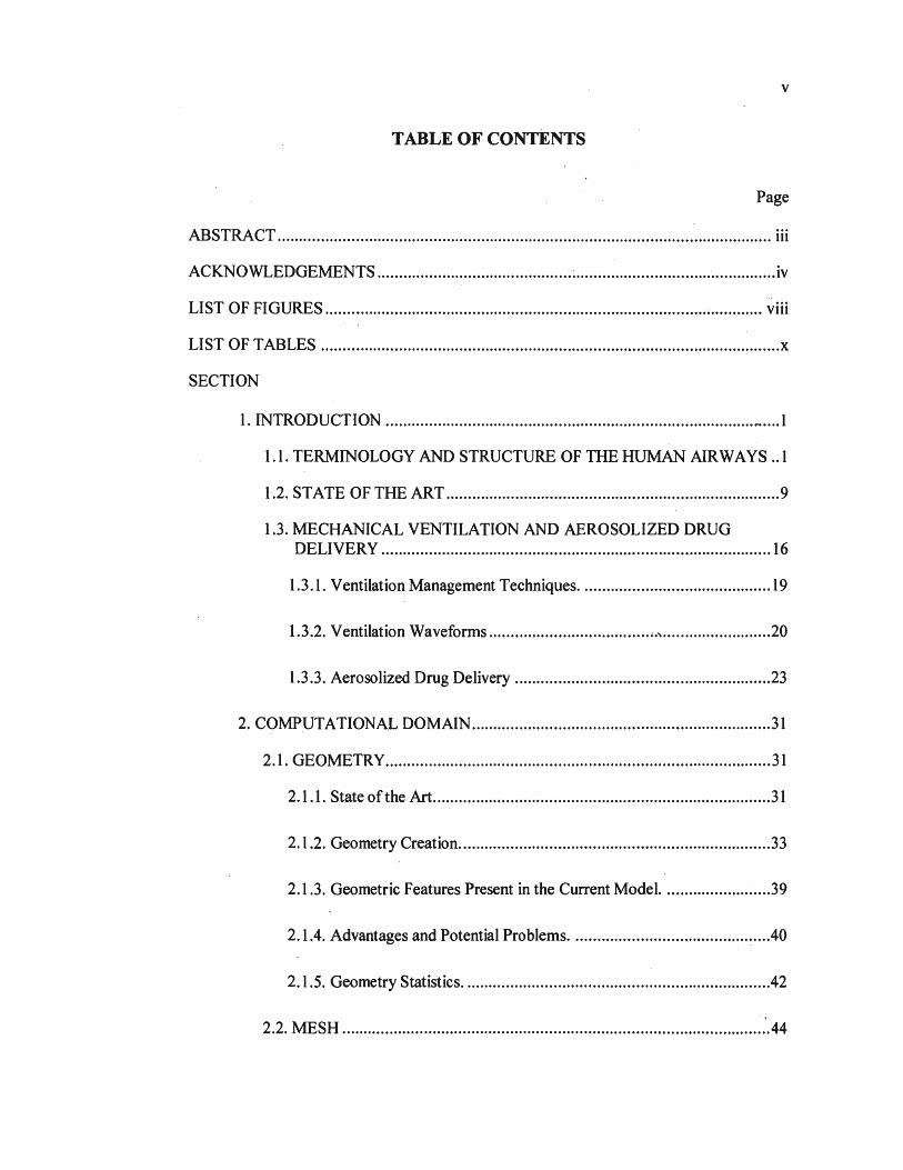
TABLE OF CONTENTS
Page
ABSTRACT ........ ~ ......................................................................................................... iii
ACKNOWLEDGEMENTS ............................................................................. -............... iv
LIST OF FIGURES .................................. ~ ..................................................... ~ ............ -viii
LIST OF TABLES .......................................................................................................... x
SECTION
1. INTRODUCTION ............................................................................................. 1
l.l. TERMINOLOGY AND STRUCTURE OF THE HUMAN AIRWAYS .. 1
1,.2. STATE OF THE ART ............................................................................. 9
1.3. MECHANICAL VENTILATION AND AEROSOLIZED DRUG DELIVERY .......................................................................................... 16
1.3 .1. Ventilation Management Techniques ............................................ 19
1.3.2. Ventilation Waveforms ..................................... ;., ......................... 20
1.3.3. Aerosolized Drug Delivery ........................................................... 23
2. COMPUTATIONAL DOMAIN ..................................................................... 31
2.1. GEOMETRY ......................................................................................... 31
2.1.1. State of the Art .............................................................................. 31
2. _1.2. Geometry ·creation ........................................................................ 33
2.1.3. Geometric Features Present in the Current Model. ........................ 3-9
2.1.4. Advantages and Potential Problems. ········································~···.40
2.1.5. Geometry Statistics ....................................................................... 42
2.2. MESH ................................................................................................... 44
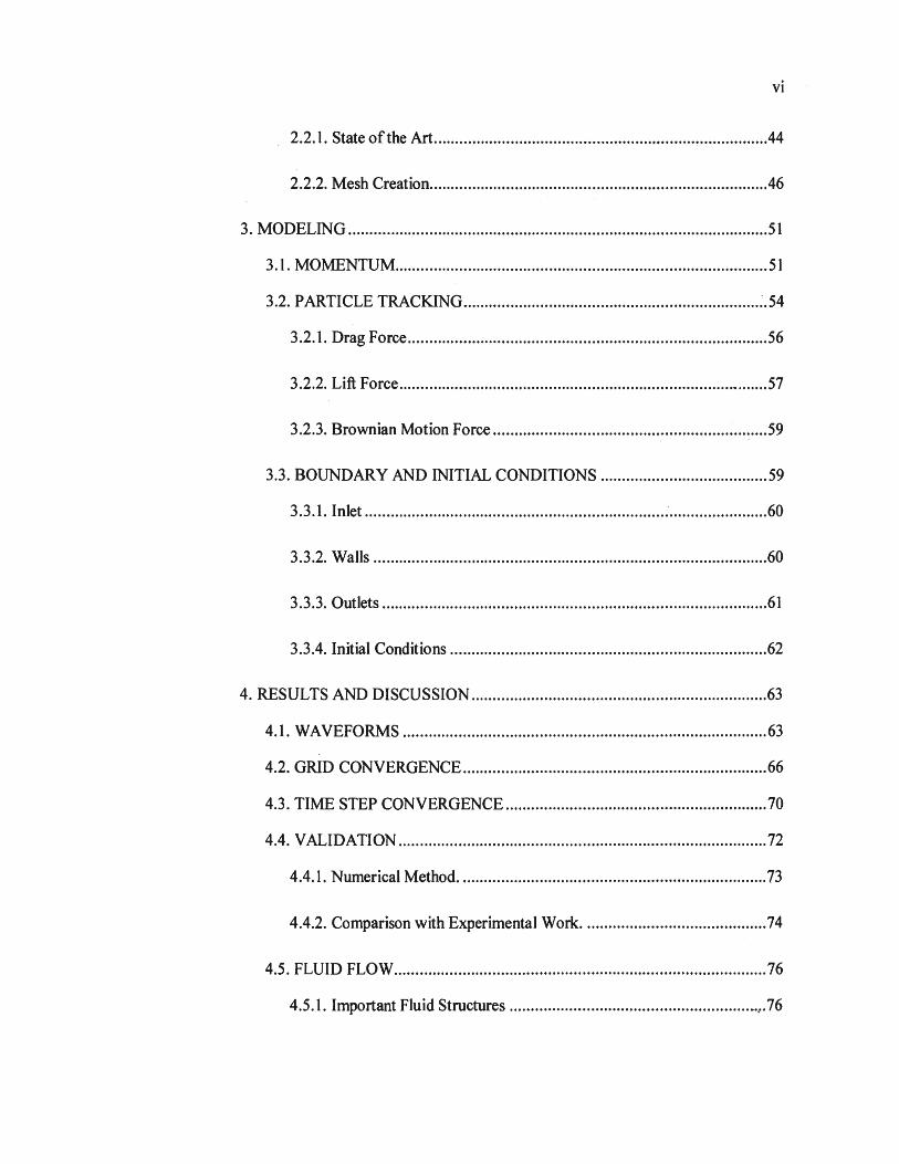
VI
2.2.1. State of the Art .............................................................................. 44
2.2.2. Mesh Creation ............................................................................... 46
3. MODELING .................................................................................................. 51
3.1. MOMENTUM ........................................................................................ 51
3.2. PARTICLE TRACKING ....................................................................... ~.54
3.2.1. Drag Forc.e .................................................................................... 56
3.2.2. Lift Force ............................................................................. - ....... 57
3.2.3. Brownian Motion Force ................................................................ 59
3.3. BOUNDARY AND INITIAL CONDITIONS ....................................... 59
3.3.1. Inlet ............................................................................................... 60
3.3.2. Walls ............................................................................................ 60
3.3.3. Outlets .......................................................................................... 61
3.3.4. Initial Conditions .......................................................................... 62
4. RESULTS AND DISCUSSION ..................................................................... 63
4.1. WAVEFORMS ..................................................................................... 63
4.2. GRID CONVERGENCE ....................................................................... 66
4.3. TIME STEP CONVERGENCE ............................................................. 70
4.4. VALIDATION ...................................................................................... 72
4.4.1. Numerical Method ........................................................................ 73
4.4.2. Comparison with Experimental Work ........................................... 74
4.5. FLUID FLOW ........................................................... ~ ........................... 76
4.5.1. Important Fluid Structures ························································ -.·· 76
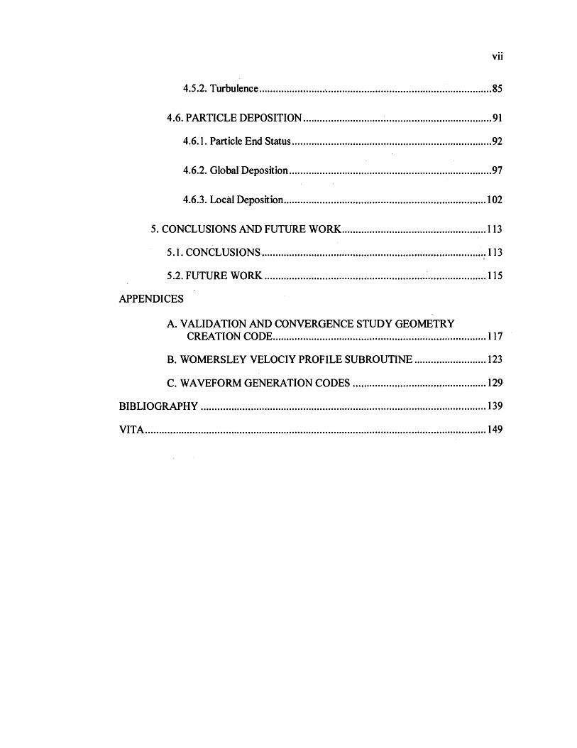
vii
4.5.2. Turbulence ..................................................................................... 85
4.6. PARTICLE DEPOSITION ............................. ~ ...................................... 91
4.6.1. Particle End Status ........................................................................ 92
4.6.2. Global Deposition.~ ........................................................... ·.~ .......... 97
4.6.3. Local Deposition ......................................................................... I 02
5. CONCLUSIONS AND FUTURE WORK .................................................... 113
5.1. CONCLUSIONS ................................................................................. 113
5.2. FUTURE WORK .......................................................... ~ ..................... 115
APPENDICES
A.VALIDATION AND CONVERGENCE STUDY GEOMETRY CREATION CODE ............................................................................. 117
B. WOMERSLEY VELOCIY PROFILE SUBROUTINE .......................... 123
C. WAVEFORM GENERATION CODES ................................................ 129
BIBLIOGRAPHY ....................................................................................................... 139
VITA ........................................................................................................................... 149
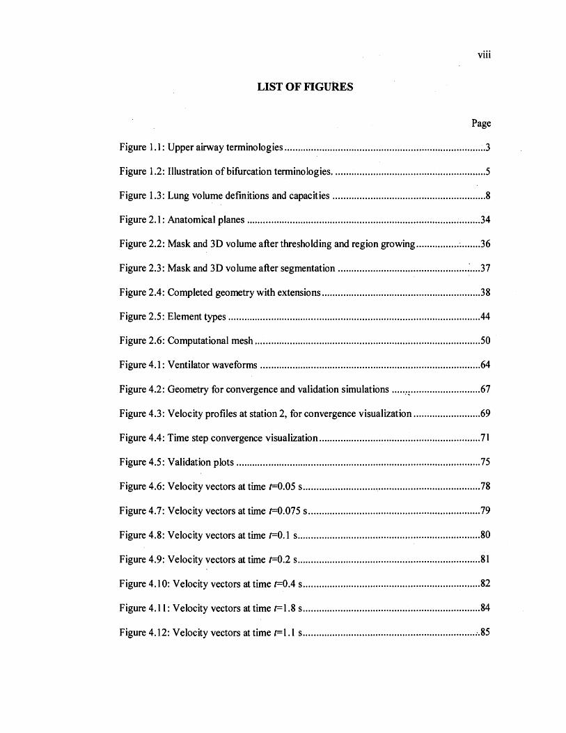
viii
LIST OF FIGURES
Page
Figure 1.1: Upper airway terminologies ........................................................................... 3
Figure 1.2: Illustration of bifurcation terminologies ....................................... ~ ................. 5
Figure 1.3: Lung volume definitions and capacities ......................................................... 8
Figure 2.1: Anatomical planes ....................................................................................... 34
Figure 2.2: Mask and 30 volume after thresholding and region growing ................ ~: ...... 36
Figure 2.3: Mask and 30 volume after segmentation ............................................... ~: .... 37
Figure 2.4: Completed geometry with extensions ........................................................... 38
Figure 2.5: Element types ............................................................................................... 44
Figure 2.6: Computational mesh .................................................................................... 50
Figure 4.1: Ventilator waveforms .................................................................................. 64
Figure 4.2: Geometry for convergence and validation simulations .... ·.·:·· ........................ 67
Figure 4.3: Velocity profiles at station 2, for convergence visualization ......................... 69
Figure 4.4: Time step convergence visualization ............................................................ 71
Figure 4.5: Validation plots ........................................................................................... 75
Figure 4.6: Velocity vectors at time t=0.05 s ........................... ~ ...................................... 78
Figure 4.7: Velocity vectors at time t=0.075 s ................................................................ 79
Figure 4.8: Velocity vectors at time t=0.1 s .................................................................... 80
Figure 4.9: Velocity vectors at time t=0.2 s .................................................................... 81
Figure 4.10: Velocity vectors at time t=0.4 s .......................................................... : ....... 82
Figure 4.11: Velocity vectors at time t=l .8 s .................................................................. 84
Figure 4.12: Velocity vectors at time t=l.1 s ................................................................... 85
ix
Figure 4.13: Contours of turbulence kinetic energy ........................................................ 87
Figure 4.14: Contours of turbulence kinetic energy ........................................................ 88
Figure 4.15: Contours of vorticity .................................................................................. 90
Figure 4.16: Contours ofvorticity ............................................. · ..................................... 91
Figure 4.17: Particle end status for different waveforms ................................................. 95
Figure 4.18: Number of particles in the domain as a function oftime ............................. 97
Figure 4.19: Deposition fraction histograms ................................................................... 99
Figure·4.20: Deposition fraction .................................................................................. 101
Figure 4.21: Deposition locations for the pressure controlled sinusoidal waveform ...... 103
Figure 4.22: Deposition locations by Stokes number .................................................... 105
Figure 4.23: Deposition locations by time .................................................................... 107
Figure 4.24: Contours of DEF (front view) .................................................................. 109
Figure 4.25: Contours of DEF (back right view) .......................................................... 110
· Figure 4.26: Contours of DEF (front left view) ............................................................ 11 l

x
LIST OF TABLES
Page
Table 2.1: Geometry information and flow ratios .......................................................... .43
Table 2.2: Comparison of diameter ratios among statistical models ............................... .43
Table 2.3: Literature review of turbulence modeling and mesh styles ............................ .46
Table 4.1: Grid convergence information ....................................................................... 68
Table 4.2: Time step convergence information ....................................................... : ....... 71
Table 4.3: Validation percent difference .................................................................... : ... 75
Table 4.4: Particle end statuses ...................................................................................... 93
Table 4.5: Overall deposition fractions .......................................................................... 98
Table 4.6: Maximum deposition enhancement factor ................................................... 112
1. INTRODUCTION
Breathing is an essential function to maintain life. Respiration is a function by
which gas exchange occurs -the body takes in oxygen from the environment and expels
carbon dioxide. The process of gas exchange involves two primary mechanisms:
conduction of gases from the external environment to the alveolar zone, and a subsequent
diffusion based exchange across the epithelium into the bloodstream [I]. Air enters the
lungs when a lower pressure is created due to the expansion of the lungs. The expansion
is controlled by a set of muscles in the thoracic cavity, most notably the diaphragm which
is located below the lungs. When the lungs prove inadequate to deliver oxygen due to
various medical conditions, mechanical ventilation is often a lifesaving intervention [2].
It is a very common therapeutic technique to deliver medicine in aerosolized form
to mechanically ventilated patients. The ability of other inhaled materials to also pass
through the epithelium into the bloodstream is what makes drug delivery in the lungs
possible. The structure of the lung has evolved to serve the function of a delivery
mechanism. For this reason it is also ideal for delivery of aerosolized drugs and at risk to
deliver inhaled toxins to the body. A better understanding of the mechanisms behind the
deposition of inhaled particulates is thus critical in improving aerosolized drug delivery
and mitigating the dangers of inhalation of airborne toxins.
1.1. TERMINOLOGY AND STRUCTURE OF THE HUMAN AIRWAYS
The human airways are a network of gas channels with complex and dynamic
features. The airways can be divided into three regions based on anatomy: (a)
extrathoracic region which includes the oral cavity, the nasal cavity, the pharynx, the
larynx, and the upper part of the trachea (b) upper bronchial region which includes the
2
bronchi, and (c) lower bronchial region which contains the bronchioles and the alveolar
region [3]. The term tracheobronchial (henceforth referred to as TB) .refers to a region
including the trachea and the upper bronchial region. With a focus on respiratory
function, it is convenient to separate the lungs into the conducting zone, and the
respiratory zone. The conducting zone contains all of the airways above the respiratory
bronchioles. The purpose of the conducting zone is to move large volumes of air from
the larger airways to the tiny airways where the flow velocity will be low enough, and
there will be enough surface area, for gas exchange to occur through the epithelium. No
gas exchange occurs in the conducting zone. Respiratory bronchioles are sometimes seen
as a transition zone where the air continues to move to lower airways but some gas
exchange does occur. The respiratory zone consists of alveolar ducts and sacs where the
primary function is gas exchange [4]. An acinus is a tiny respiratory unit that consists of
a primary respiratory bronchiole and all of the respiratory bronchioles, alveolar ducts, and
alveolar sacs it supplies [5].
Air that enters through the mouth will pass through the oral cavity into the
pharynx. The pharynx acts as a pipe junction as it connects to the nasal cavity, oral
cavity, larynx, and ·esophagus. It is broken into three parts: (1) the nasopharynx which
connects to the nasal cavity and leads into (2) the oropharynx which connects to the oral
cavity and leads into (3) the laryngopharynx (sometimes called the hypopharynx) which
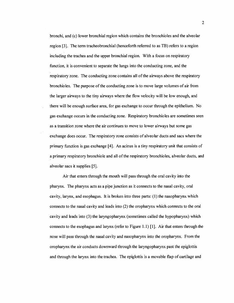
connects to the esophagus and larynx (refer to Figure I.I) [I]. Air that enters through the
nose will pass through the nasal cavity and nasopharynx into the oropharynx. From the
oropharynx the air conducts downward through the laryngopharynx past the epiglottis
and through the larynx into the trachea. The epiglottis is a movable flap of cartilage and
tissue that covers the opening of the larynx to direct food or drink down t,he esophagus
while swallowing [ 6]. The larynx leads into the trachea and contains the glottis [ 6].
I ph. r nx
Hypoph rynx
Ew pha u~
mu
ity
- --- ~ ----- Sahvary gland
rach .:a
Figure 1.1: Upper airway terminologies [7]
Beginning from the trachea, the lungs split repeatedly. The trachea splits into the
left and right main bronchi which split into the lobar bronchi. The left lung contains two
lobes, referred to as the left upper and lower lobes; whereas the right lung consists of
three lobes that are referred to as the right upper, middle, and lower lobes [1]. The lobar
bronchi continue to split into the tertiary bronchi, each of which supplies a broncho
pulmonary segment (BPS) [8]. A BPS is a segment of the lung that is supplied by its
3

4
own blood vessels and is separated from the other segments by connective tissue. The
BPSs contain the bronchioles and alveolar ducts and sacs, and mark the end of the
bronchi. The primary bronchioles (i.e. the first airways in each BPS) continue to split
repeatedly until the terminal bronchioles which supply the respiratory bronchioles and are
considered to be the most distal airways (farthest from the stem, or trachea). The
respiratory bronchioles contain alveoli, but also continue to split and supply alveolar
ducts and sacs where gas exchange primarily takes place.
The airways after each bifurcation ( or split) are considered to be in a new
generation and the number of airways in each generation is approximately double that of
the previous generation. The lungs are made up of about 23 generations of branching
airways with the trachea as the 0th generation (GO), the left and right main bronchi as the
1st and so on [5]. The bronchioles begin at generations 3 or 4 and continue through
generations 16 to 19 [5]. The alveolar ducts are only present for about 4 generations after
the respiratory bronchioles. The airways terminate at the alveolar sacs. A bifurcation
primarily consists of a parent branch that splits into two daughter branches. A parent
branch is considered to be proximal (closer to the trachea) to the daughter branch and the
daughter branches are considered to be distal (farther from the trachea) to the parent
branch. In general the size of the parent branch is larger than that of its daughter
branches with few exceptions [5]. The size of an airway could be characterized by a
diameter; however the airways are not perfectly round. For this reason· it is convenient to
define a hydraulic diameter (Dh) to characterize the size of an airway as:
D _ 4A
h- p (I.I)

5
where A is the cross sectional area, and P is the wetted perimeter of a slice, cut
perpendicular to the center line of the airway. It should be noted that the hydraulic
diameter for the pulmonary airways is not strictly constant along the axis of an airway but
rarely varies significantly. The branch angle is the angle between the two daughter
branches of a bifurcation, the ridge-like area where the parent branch separates being
called a carina. Figure 1.2 illustrates some of the commonly used terminologies that are
used to quantify pulmonary bifurcations.
Branch Angle
Parent Branch
Figure 1.2: Illustration of bifurcation terminologies.
The lining of the airways is known as an epithelium. In the alveoli, the
epithelium is comprised of type I and type II epithelial cells. Type I epithelial cells make
up about 97% of the alveolar surface and their primary function is gas exchange. Type II
epithelial cells are responsible for secreting a surfactant that increases the airway
compliance, prevents atelectasis (lung collapse), and helps keep the alveoli dry [5]. The
6
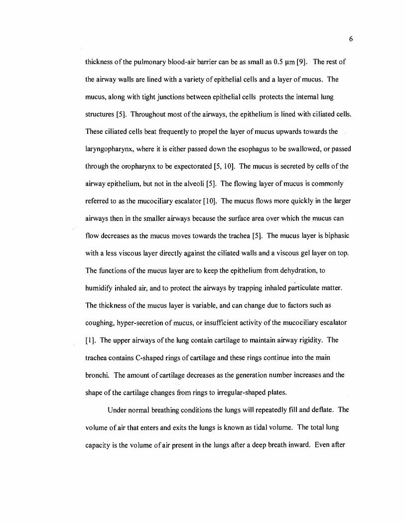
thickness of the pulmonary blood-air barrier can be as small as 0.5 µm [9]. The rest of
the airway walls are lined with a variety of epithelial cells and a layer of mucus. The
mucus, along with tight junctions between epithelial cells protects the internal lung
structures [5]. Throughout most of the airways, the epithelium is lined with ciliated cells.
These ciliated cells beat frequently to propel the layer of mucus upwards towards the
laryngopharynx, where it is either passed down the esophagus to be swallowed, or passed
through the oropharynx to be expectorated (5, 1 O]. The mucus is secreted by cells of the
airway epithelium, but not in the alveoli [5]. The flowing layer of mucus is commonly
referred to as the mucociliary escalator (10]. The mucus flows more quickly in the larger
airways then in the smaller airways because the surface area over which the mucus can
flow decreases as the mucus moves towards the trachea [5]. The mucus layer is biphasic
with a less viscous layer directly against the ciliated walls and a viscous gel layer on top.
The functions of the mucus layer are to keep the epithelium from dehydration, to
.. humidify inhaled air, and to protect the airways by trapping inhaled particulate matter.
The thickness of the mucus layer is variable, and can change due to factors such as
coughing, hyper-secretion of mucus, or insufficient activity of the mucociliary escalator
[I]. The upper airways of the lung contain cartilage to maintain airway rigidity. The
trachea contains C-shaped rings of cartilage and these rings continue into the main
bronchi. The amount of cartilage decreases as the generation number increases and the
shape of the cartilage changes from rings to irregular-shaped plates.
Under normai breathing conditions the lungs will repeatedly fill and deflate. The
volume of air that enters and exits the lungs is known as tidal volume. The total lung
capacity is the volume of air present in the lungs after a deep breath inward. Even after
7
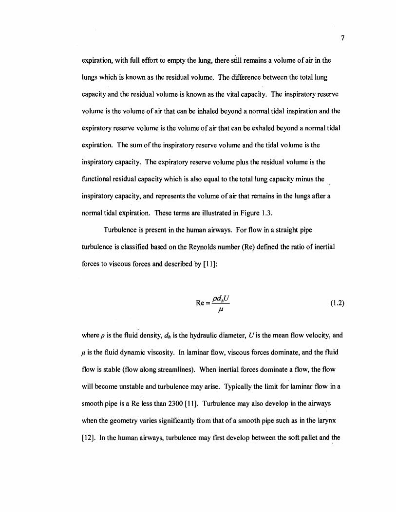
expiration, with full effort to empty the lung, there still remains a volume of air in the
lungs which is known as the residual volume. The difference between the total lung
capacity and the residual volume is known as the vital capacity. The inspiratory reserve
volume is the volume of air that can be inhaled beyond a normal tidal inspiration and the
expiratory reserve volume is the volume of air that can be exhaled beyond a normal tidal
expiration. The sum of the inspiratory reserve volume and the tidal volume is the
inspiratory capacity. The expiratory reserve volume plus the residual volume is the
functional residual capacity which is also equal to the total lung capacity minus the
inspiratory capacity, and represents the volume of air that remains in the lungs after a
normal tidal expiration. These terms are illustrated in Figure 1.3.
Turbulence is present in the human airways. For flow in a straight pipe
turbulence is classified based on the Reyno Ids number (Re) defined the ratio of inertial
~orces to viscous forces and described by [ 11]:
Re= pdhU µ
(1.2)
where p is the fluid density, dh is the hydraulic diameter, U is the mean flow velocity, and
µ is the fluid dynamic viscosity. In laminar flow, viscous forces dominate, and the fluid
flow is stable (flow along streamlines). When inertial forces dominate a flow, the flow
will become unstable and turbulence may arise. Typically the limit for laminar flow in a
smooth pipe is a Re less than 2300 [11]. Turbulence may also develop in the airways
when the geometry varies significantly from that of a smooth pipe such as in the larynx
(12]. In the human airways, turbulence may first develop between the soft pallet and the

throat [ 13] and after the larynx, but will re-laminarize in the lower airways where the
Reynolds number is lower [14]. Turbulence is expected in the airways from generation
GO Gust after the larynx) and may be present up to generation G6 [13].
7
0
Inspiratory Reserve Volume
- -Tidal Volume r--
Expiratory Reserve Volume
Residual Voh.lme . t ____ _
Vital Capacity
Total Lung
Capacity
Functional Residual Capacity
8
Figure 1.3: Lung volume definitions and capacities. This figure is adopted from ref. f 5].
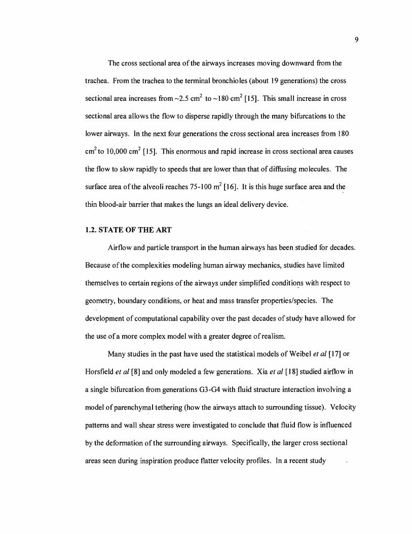
The cross sectional area of the airways increases moving downward from the
trachea. From the trachea to the terminal bronchioles ( about 19 generations) the cross
sectional area increases from -2.5 cm2 to -180 cm2 [ 15]. This small increase in cross
sectional area allows the flow to disperse rapidly through the many bifurcations to the
lower airways. In the next four generations the cross sectional area increases from 180.
cm2 to 10,000 cm2 [ 15]. This enormous and rapid increase in cross sectional area causes
the flow to slow rapidly to speeds that are lower than that of diffusing molecules. The
surface area of the alveoli reaches 75-100 m2 [16]. It is this huge surface area and the
thin blood-air barrier that makes the lungs an ideal delivery device.
1.2. STATE OF THE ART
9
Airflow and particle transport in the human airways has been studied for decades.
Because of the complexities modeling human airway mechanics, studies have limited
themselves to certain regions of the airways under simplified conditi<?1:)S with respect to
geometry, boundary conditions, or heat and mass transfer properties/species. The
development of computational capability over the past decades of study have allowed for
the use of a more complex model with a greater degree of realism.
Many studies in the past have used the statistical models of Weibel et al [17] or
Horsfield et al [8] and only modeled a few generations. Xia et al [ 18] studied airflow in
a single bifurcation from generations G3-G4 with fluid structure interaction involving a
model of parenchymal tethering (how the airways attach to surrounding tissue). Velocity
patterns and wall shear stress were investigated to conclude that fluid flow is influenced
by the deformation of the surrounding airways. Specifically, the larger cross sectional
areas seen during inspiration produce flatter velocity profiles. In a recent study
IO
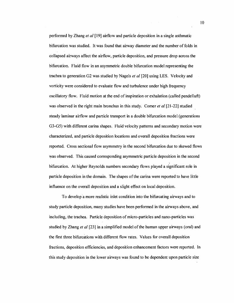
performed by Zhang et al [19] airflow and particle deposition in a single asthmatic
bifurcation was studied. It was found that airway diameter and the number of fo Ids in
collapsed airways affect the airflow, particle deposition, and pressure drop across the
bifurcation. Fluid flow in an asymmetric double bifurcation model representing the
trachea to generation 02 was studied by Nagels et al [20] using LES. Velocity and
vorticity were considered to evaluate flow and turbulence under high frequency
oscillatory flow. Fluid motion at the end of inspiration or exhalation (called pendelluft)
was observed in the right main bronchus in this study. Comer et al [21-22] studied
steady laminar airflow and particle transport in a double bifurcation model (generations
03-05) with different carina shapes. Fluid velocity patterns and secondary motion were
characterized, and particle deposition locations and overall deposition fractions were
reported. Cross sectional flow asymmetry in the second bifurcation due to skewed flows
was observed. This caused corresponding asymmetric particle deposition in the second
bifurcation. At higher Reynolds numbers secondary flows played a significant role in
particle deposition in the domain. The shapes of the carina were reported to have little
influence on the overall deposition and a slight effect on local deposition.
To develop ·a more realistic inlet condition into the bifurcating airways and to
study particle deposition, many studies have been performed in the airways above, and
including, the trachea. Particle deposition of micro-particles and nano-particles was
studied by Zhang et al [23] in a simplified model of the human upper airways (oral}and
the first three bifurcations with different flow rates. Values for overall deposition
fractions, deposition efficiencies, and deposition enhancement factors were reported. In
this study deposition in the lower airways was found to be dependent upon particle size
11
distributions which in tum are dependent upon upstream deposition. The non-uniformity
of particle deposition was found to be higher for larger particle diameters with micro
particle deposition highly non-uniform, nano-particle deposition more uniform, and with
ultrafine particles depositing over a very large area. Longest eta/ [24] studied nano
particle deposition in a simplified model of the oral airways from the mouth to the
trachea using both Lagrangian and Eulerian methods for particle tracking. This study
also compared particle tracking models in a commercial software package to user defined
models. Calculation of deposition fraction and deposition enhancement factors helped to
characterize the differences in the built in and user defined models as well as the
differences between the Lagrangian and Eulerian models. When compared to
experimental studies the use of the Lagrangian model with the user defined models
showed much better agreement than the built in models which stresses the importance of
an appropriate Lagrangian particle tracking model. The Eulerian model also showed a
similar degree of agreement with experimental studies; however the Lagrangian and
Eulerian models still showed significant differences with each other, which was
hypothesize_d to be due to slip corrections. Targeted drug aerosol delivery was studied by
Kleinstreuer et al [25] in a simplified model of the upper airways from the mouth to
generation G3 using a Weibel symmetric and asymmetric model. Particle termination
locations were determined using a Lagrangian particle tracking method and the starting
positions of those particles at the inlet of the oral airways were presented as release sites
for drug aerosol targeting. A proof of concept experimental study was also performed in
a physical reproduction of the computational airway model. Cross sectional particle
distributions are presented to compare experimental and predicted particle transport

12
through the domain. Visually, the experimental data was reported to agree well with
simulation data. The capture efficiency, which characterizes the percentage of particles
reaching the prescribed target zone, varied greatly from 10 % to 100 % with higher
values at low flow rates and lower values under normal breathing conditions. Secondary
flows were found to play a significant role in the stretching and squeezing of the initial .
particle bolus released at the inlet. Xi et al [26] studied the effects of simplified models
on particle deposition in the oral airway. Four models were generated: a realistic one
directly from CT scans, one with elliptical cross sections, one with circular cross sect_ions,
and one with circular cross sections with a constant diameter. Deposition fractions,
deposition locations, deposition enhancement factors, and particle profiles at the exit
(trachea) were used to compare the four models. The best agreement of deposition
fraction with other experimental studies was found with the realistic airway model,
~lthough the deposition fractions for all four models fell within one standard deviation of
experimental data. Despite the agreement of the airway models with respect to overall
deposition fractions, differences in the local deposition characteristics were found to be
much more significant. Airflow and particle transport through a tube with a local
constriction and a simplified model of the oral airways from the mouth to the trachea was
studied by Zhang et al [27]. Comparisons were made between an LES turbulence model
and three Reynolds averaged Navier-Stokes models: k-co model, low Reynolds number k
co model, and the shear stress transport transition model. Velocity and turbulence kinetic
energy were evaluated and compared between the turbulence models and compared to
experimental data. The general trend of the turbulence dissipation was similar between
the tube with a local constriction and the oral airway model, but the oral airway model
13
had significantly more complex airflow structures. It was concluded that local
constrictions were the dominant geometric feature responsible for producing turbulence.
The standard k-ro model failed to capture laminar behavior at low Reynolds numbers,
while little difference was found between the other three models. The ability of LES to
capture instantaneous velocity fluctuations was hypothesized to be important for
modeling mico-particle transport.
In recent years, due to advancements in medical imaging equipment and
techniques, studies have begun to use geometries based on CT scans of patients. Choi et
al [28] studied airflow through geometries created from the CT scans of two patients
from the mouth to generation 07. Velocities, turbulence kinetic energy, and turbulent
coherent structures were compared between the subjects to assess inter-subject
variability. It was concluded that airflow structures at similar flow rates were only
qualitatively similar and the differences in flow characteristics between the subjects was
attributed to the glottal aperture area and the shape and orientation of the trachea.
Simulations were also run in the geometry of one patient with the complete model and
three models at different truncation levels to investigate intra-subject variability.
Truncated geometries resulted in the absence of some of the major airflow structures.
Careful analysis of proposed improved boundary conditions for the truncated geometries
showed solutions that were closer to those obtained with the full geometry. Inthavong et
al [29] studied airflow and micro-particle deposition in a model generated from CT scans
of a patient from the trachea to generation GS. Two breathing conditions were applied at
the inlet: the first half a sinusoidal waveform over 2 seconds with a peak inspiratory flow
rate of90 L/min with a 2 second breath hold immediately after, and 5 cycles of a

14
sinusoidal waveform over 10 seconds (2 seconds per cycle) with a peak inspiratory flow
rate of 30 L/min. Fluid flow was characterized with velocity contours and secondary
flows vectors at slices throughout the domain. Secondary flow vortices were seen in the
domain and were stronger during inspiration. Deposition fractions were used to
characterize the particle depositions for both breathing conditions. Increased deposition
fractions were reported for the breathing condition with the higher flow rate and breath
hold. Analysis of the deposition patterns revealed that the breathing condition with the
breath hold and higher flow rate increased deposition in the first few bifurcations ins~ead
of in the lower generations. Fluid flow and particle deposition was studied by Xi et al
[30] in a model from CT scans with and without a larynx. Fluid flow was characterized
with velocity profiles, and turbulence viscosity ratios as well as velocity contours, and
secondary motion vectors in slices through the domain. The laryngeal jet was found to
cause a large region of recirculating flow in the trachea and to generate turbulence.
Particle deposition was characterized with particle deposition locations, particle
deposition fractions, particle deposition enhancement factors, particle trajectories, and
cross sectional particle profiles. The larynx was shown to be important for modeling
fluid flow and particle transport in the upper airways causing a decreased deposition at
the carina of the first bifurcation and the first three bronchi, increased deposition in the
trachea, and increased particle transport to the lower airways of the model. In a recent
study by Lambert et al [31] fluid flow particle deposition was studied in a CT scan based
model of the airways from the mouth to generation G7 using large eddy simulation for a
steady inlet condition. An assessment of velocity, and turbulence kinetic energy, particle
deposition locations, deposition fractions and efficiencies, and particle transport profiles
showed that the laryngeal jet was a great influence in particle impaction and dispersion.
The left lung was found to have grater deposition which was thought to be caused by
airway geometry and influences of the laryngeal jet flow in the trachea.
15
Before the widespread availability of high computing power, experiments were
often more useful in the study of fluid flow and particle deposition in the human airways.
In recent years the number of experimental studies being performed has dropped but
there is a great deal of insight yet to be gained from experimental studies and with
advancements in computational model realism there will be an increased importance. for
experimental data for validation and for setting realistic boundary data. GroBe et al [32]
experimentally studied airflow in a silicone cast of generations GO-G6. PIV was used
with hydrogen bubbles in a water glycerin mixture to take measurements of the flow
field. Velocity vectors and contours, vorticity contours, and ail analysis ofvortical
structures were presented to carefully study the flow in the first bifurcation. Vortical
flow structures were found to depend strongly on the Reynolds number and Womersley
number. Fully developed flow was not seen in any of the bronchial generations,
indicating the importance of ensuring proper flow rate distributions. Transient evolution
of bronchial flows was observed under oscillating flow conditions that would not
otherwise be captured with steady state analyses. In an experiment by Zhang et al [33]
the effects of cartilaginous rings on particle deposition was studied in two simplified
models from the mouth to generation G3 with a symmetric in plane triple bifurcation: one
with a representation of cartilaginous rings, and one without. Particle deposition was
measured by determining the increase in mass of the filters that were placed at the outlets
to capture particles. Deposition fractions and deposition efficiencies were presented.

16
The inclusion of cartilaginous rings was found to greatly increase the deposition
efficiencies. Experiments were performed by Fresconi et al [34] in a symmetric planer
triple bifurcation model under oscillatory flow conditions. PIV measurements were made
using fluorescent particles in a glycerol-water solution to collect data on secondary flow
velocities. Centrifugal forces were shown to trigger secondary flows including Dean
vortices due to the curvature in the airways. It was hypothesized that Dean vorticies may
be present up to generations 10-13 depending on inspiratory flow conditions. Due to the
repeated interruption of flow development by each new bifurcation secondary flow
velocities did not exceed 20 % of the primary flow velocities in the airways. In addition,
local curvature was found to have a greater effect on secondary flows than the
propagation of flow fields from higher generations. Kim et al [35] studied particle
deposition in a symmetric planar double bifurcation and a symmetric double bifurcation
with the second bifurcation oriented 90° out of plane. Particle depositions were
determined by 4issolving deposited uranine particles in water and measuring the
concentrations with a fluorometer. The model was divided into several sections and
filters were placed at the outlets so that regional deposition efficiencies could be
determined. Valves were also placed at the outlets so that the flow distribution could be
adjusted. Deposition fraction and deposition efficiency values showed that the angular
position of the bifurcations as well as the flow distributions had a significant impact on
region particle deposition.
1.3. MECHANICAL VENTILATION AND AEROSOLIZED DRUG DELIVERY
Mechanical ventilation is a mechanical means to assist or replace a patient's
natural breathing. It is now the most commonly used mode of life support in medicine
17
[36]. Mechanical ventilation is used when a patient's natural breathing is not sufficient to
deliver oxygen to the bloodstream. Common indications for mechanical ventilation
include acute lung injury (ALI), acute respiratory distress syndrome (ARDS), acute
respiratory failure (ARF), acute exacerbation of chronic obstructive pulmonary disease
(COPD), severe asthma, cystic fibrosis, pulmonary edema, pulmonary embolus, coma,
drug overdose, neuromuscular disorders, and others [37-39]. Many diseases which
require drug treatment are also indications for ventilation such as COPD, ARDS, and
severe asthma [5]. For this reason it is logical to deliver drugs directly to the lungs in
aerosolized form while undergoing mechanical ventilation treatment. The use of
pharmaceutical aerosols is advantageous for several reasons. The surface area of the lung
epithelium available for drug absorption is very large (75-100 m2) which is much greater
than that of the gastro-intestinal (GI) system [5]. In addition the epithelium is very thin
(0.5 µm) which allows for rapid drug absorption [14]. Unlike ingestion, the blood will
flow to the rest of the body before passing through the liver. When considering the
application of systemic drugs, injection is used more frequently than inhaled aerosols for
drug delivery. However in recent years the use of inhaled drug aerosols for systemic
delivery has also increased and it has shown improvement even over subcutaneous
injection of insulin [40]. Continued advances in drug aerosol delivery may make the
lungs a more viable delivery method.
The effectiveness of pulmonary drug delivery under mechanical ventilator
conditions is dependent on a number of factors [ 41-42] that are itemized below:
(a) Ventilator related: Ventilation mode, tidal volume, respiratory rate, duty cycle,
inspiration waveform and breath-triggering mechanism
(b) Circuit related: Endotracheal tube size, humidity and density of inhaled gas
18
(c) Device related: Type of device (nebulizer, metered dose inhaler, or dry powder
inhaler), fill-volume, gas flow, cycling (inspiration vs. continuous), duration, and timing
of actuation
( d) Drug related: Dosage, formulations, particle size, targeted site for delivery and
duration
(e) Patient related: Age, ethnicity, severity of airway obstruction, mechanism of
obstruction, presence of dynamic hyper-inflation and patient ventilator synchrony
The objective of this study is to explore the ventilator related effects on
pulmonary drug delivery. Specifically we focus on the waveforms of the respiratory
cycle as they are easily adjusted on modem ventilators. In this study, the focus is on the
model of a single patient and not intra-subject variability. For this reason the factors that
fall into the patient related category will not be discussed further.
Mechanical ventilation can be lifesaving, but there are also risks and potential
complications associated with mechanical ventilation. These risks and complications
include but are not limited to: infections, obstructions, ventilator induced lung injury
(VILI), and damage to the trachea due to the endotracheal tube or airtight cuffs. VILI is
actually a set of conditions that can be caused by volutrauma (damage to the lungs due to
over-inflation of the lungs), barotrauma (damage due to excessive pressures),
atelectrauma (damage from repetitive opening and collapse of distal airways), or
biotrauma (severe inflammation of the lungs) [43]. In addition if the ventilation is not

19
properly controlled then the pH levels of the blood may increase (respiratory alkalosis) or
decrease (respiratory acidosis) [5].
1.3.1. Ventilation Management Techniques. Mechanical ventilators can be
separated into two main groups: (a) negative pressure ventilators, and, (b) positive
pressure ventilators. Negative pressure ventilators create suction outside of the thoracic
cavity which creates a pressure differential that causes air to move into the lungs.
Positive pressure ventilators push air into the lungs by creating a higher pressure in an
endotracheal tube, or outside the nose or mouth causing air to flow into the lungs. Tt1e
use of negative pressure ventilators has decreased dramatically and they are rarely seen in
use at modem hospitals [44]. This study does not focus on negative pressure ventilation.
It is important to note, however, how positive pressure ventilation is different from
normal breathing [45].
Normal breathing is controlled by a set of muscles and the natural compliant
properties of the lungs. Muscles in the thoracic cavity (most notably the diaphragm
muscle) work to expand the lungs. The expansion of the lungs causes a decrease in
airway pressure and the pressure differential between the airway pressure and the ambient
( external) pressure is what drives the flow of air into the lungs during inspiration. During
exhalation the muscles relax and allow the lung to return to its natural size. This process
is passive and is driven by the natural elasticity of lung tissue. The pressure in the
airways increases and the pressure differential between the airway pressure and the
ambient pressure is what drives the flow of air out of the lungs.
Some patients are unable to produce any respiratory effort and the ventilator must
provide the total effort of breathing. This type of ventilation is known as controlled
20
mechanical ventilation (CMV) and is used for patients that are, for example, comatose, or
on anesthesia [36]. Other patients are able to produce some respiratory efforts, however
their efforts are not sufficient to supply oxygen properly, or their efforts are not
consistent. This type of ventilation is called assisted mechanical ventilation (AMV) and
the ventilator input is triggered by the patient's inspiratory effort based on a measurement
of flow or pressure. It is common for ventilators to offer an assist-control mode, where
the ventilator will assist when inspiratory effort is detected and deliver a controlled breath
when inspiratory effort is absent, usually based on a time trigger [36].
Traditionally, there are four phases of the ventilator cycle: trigger, delivery, cycle,
and expiration [36]. The trigger phase marks the onset of inspiration. Even under CMV
there is some trigger that initiates inspiration such as flow or time. Triggers are generally
based on time, flow, or pressure. After the trigger has been set a breath is delivered by
the ventilator. There are many risks involved with improper breath delivery (discussed
above) so the inspiratory waveform must be precisely controlled. The delivery phase will
be discussed further in § 1.3 .2. The cycle phase marks the end of inspiration and the onset
of exhalation. The cycle phase is generally detected by measurements of pressure,
volume, time, or volumetric flow rate. The expiration phase is a passive process of
allowing the natural elasticity of the lungs to force air out of the lungs [46]. This phase
closely resembles expiration during natural breathing with the exception of additional
flow resistance due to the ventilator circuit [ 4 7]. Expiration is allowed to occur naturally
until the next trigger phase which marks the beginning of the next breath cycle [ 4 7].
1.3.2. Ventilation Waveforms The artificial breathing during positive pressure
mechanical ventilation needs to be carefully controlled to avoid VILI but still maintain
21
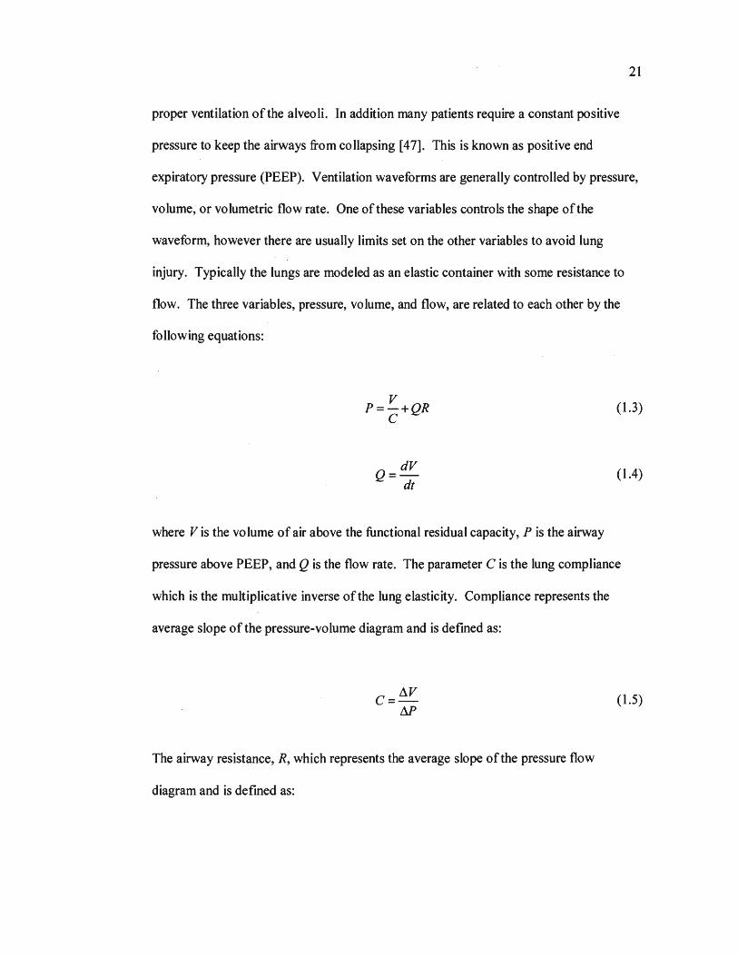
proper ventilation of the alveoli. In addition many patients require a constant positive
pressure to keep the airways from collapsing [47]. This is known as positive end
expiratory pressure (PEEP). Ventilation waveforms are generally controlled by pressure,
volume, or volumetric flow rate. One of these variables controls the shape of the
waveform, however there are usually limits set on the other variables to avoid lung
injury. Typically the lungs are modeled as an elastic container with some resistance to
flow. The three variables, pressure, volume, and flow, are related to each other by ~he
following equations:
v P=-+QR c
Q=dV dt
where Vis the volume of air above the functional residual capacity, Pis the airway
(1.3)
(1.4)
pressure above PEEP, and Q is the flow rate. The parameter C is the lung compliance
which is the multiplicative inverse of the lung elasticity. Compliance represents the
average slope of the pressure-volume diagram and is defined as:
(1.5)
The airway resistance, R, which represents the average slope of the pressure flow
diagram and is defined as:

22
(1.6)
Although, lung compliance (C) and airway resistance (R) are not constant for a given
patient nor throughout a complete respiratory cycle, it is a common assumption to
consider them to have a constant value when evaluating waveform patterns [ 48].
Ventilators can be classified into three types depending on what variables they use
to control the inspiratory waveform. Although it is very common for a ventilator ~Q offer
different types of control it cannot simultaneously control all three variables (pressure,
volume, and flow) [47]. A pressure controller will set the delivered pressure throughout
inspiration though this set pressure need not be a constant pressure. The flow rate and
volume throughout the cycle depend on the airway resistance and compliance as can be
seen in Equation 1.3. A volume controller will set the volume of air delivered throughout
inspiration. There are ventilators that integrate flow measurements to determine volume,
but a true volume controller will measure volume by the displacement of a piston or
bellows and use this measurement to control breath delivery [47]. Because flow is the
time derivative of volume and there are no other constants involved (Equation 1.3), the
flow is also determined when the volume is set. The, pressure, however will depend
upon the airway resistance and compliance as can be seen in Equation 1.2. A flow
controller will set the flow of air throughout inspiration. The volume is the integral of
flow with no other constants involved which can be seen in Equation 1.3. This means
that the change in the volume of the lung from the volume at the onset of inspiration will
also be determined when the flow is set. Therefore if the functional residual capacity
remains constant each cycle, then the same flow waveform will produce the same vo l1.:1me

23
waveform regardless of changes in lung compliance and airway resistance. The pressure
throughout the inspiration phase for a flow controller will depend on the lung compliance
and airway resistance as can be seen in Equation 1.2.
Pressure control is considered to be more protective ventilation strategy than
volume or flow control, but because the volume depends on the compliance and
resistance there is no guarantee that the degree of ventilation will be sufficient or
necessary [36]. Volume and flow control will deliver a set amount of air to the lun~s, but
because pressure depends on the compliance and resistance there is a higher risk of .
barotrauma or airway closure. When set up properly, volume control, flow control, and
pressure control will be equally sufficient in providing gas exchange, hemodynamics, and
pulmonary mechanics [36].
The effect of the waveforms on pulmonary drug delivery may be more significant
than the effects on alveolar ventilation. The aerosolized particles suspended in the flow
are not the same density as the flowing air and will not simply follow along with the
flow. Fluid flow characteristics influence the degree and location of particle deposition
[49]. The speed of the flow will have a direct influence on particle deposition and there
are additional influences due to turbulent eddies in the domain.
1.3.3. Aerosolized Drug Delivery Mechanical ventilation is meant as a
temporary intervention to assist in breathing but does not cure any underlying disease
[50]. Aerosolized drug delivery can help to keep the airways fit for oxygen delivery and
carbon dioxide expulsion, and can help to treat the underlying conditions. It is also being
used for insulin delivery, pain management, cancer therapy, and nanotherapeutics [ 14].
24
There ·are several commonly used drug aerosol treatments. Bronchodilators are
used to open airways in patients with asthma and chronic bronchitis [5]. In general they
are used to relax the muscles in the rings around the airways causing the airways to
widen. Corticosteroids are used to reduce inflammation in airways for patients with
asthma or emphysema [5]. Aerosolized antibiotics are used to treat broncho.;.pulmonary
infections and are especially useful for patients with cystic fibrosis, who are susceptible
to pulmonary infections [51). Ipratropium bromide is used to reduce the production of
mucus in chronic bronchitis [52). Mucolytic agents are used to reduce the viscosity of
mucus for patients with COPD [5]. This will make mucus clearance easier and reduce
the obstructions in the airways. Insulin therapy is also being considered as an aerosol
therapy that has shown improvement over traditional subcutaneous injection [ 40).
Drug aerosols are delivered by one of three devices: nebulizers, metered dose
inhalers (MDI), or dry powder inhalers (DPI). Nebulizers are a device to aerosolize
liquid medications. There are three types of common nebulizers: (a) jet nebulizers, (b)
ultrasonic nebulizers, and, ( c) vibrating mesh nebulizers. Jet nebulizers use a jet of air
that entrains liquid medications. The entrained fluid thins out in the air stream until it
forms instabilities. These instabilities continue to stretch and thin until breakup occurs.
The particles form due to surface tension [42). The airstream is passed by a baffle that
causes larger particles to impact and move to the walls while smaller particles will flow
past. The air jet required for these nebulizers can come from compressed air or can be
generated by an electric compressor. These devices tend to be bulky and must have a
source of compressed air or electricity depending on the model.

25
Ultrasonic nebulizers use a piezoelectric at the bottom of the liquid medicine
reservoir to create ultrasonic vibrations in the liquid. The vibration waves travel to the
surface where instabilities occur. The instabilities grow, stretch, and thin until particle
breakup occurs. The particles form due to surface tension. These devices require a
source of electricity. In ultrasonic and jet nebulizers particles that are small enough to be
suspended in the airstream are passed out of the nebulizer to the ventilator circuit to be
delivered to the patient. Particles that are too large will drop down into the medicat.ion
reservoir or collect on the walls and be recycled. Vibrating mesh nebulizers use a mesh
attached to a piezoelectric. The mesh is full of tapered holes that act as micro pumps as
the mesh vibrates. As the mesh moves into the fluid, the fluid is forced through the holes
forming tiny droplets. These devices require electricity but can be battery powered [42].
Unlike jet and ultrasonic nebulizers, vibrating mesh nebulizers do not recycle aerosolized
medication [53]. These devices require precision holes which can increase cost. In
addition they may be difficult to disinfect. Metered dose inhalers (MDI) are portable
drug delivery devices that are specifically designed to deliver a precise dose to the
patient. They are comprised of a canister, a propellant, medication (either liquid or
particles suspended in liquid), a metering valve, and an actuator. The canister contains
the medicine formulation and the propellant. When actuated, the propellant will force the
drug formulation through the metering valve which controls the dose. The formulation
will begin to expand and boil. Liquid ligaments will form and will be ripped apart by
aerodynamic forces forming particles [54]. The patient's breath must be synchronized
with the actuation to achieve proper delivery. The propellant causes the aerosolized
medicine to leave the device at a high velocity which can cause a high degree of

26
deposition in the oropharynx. Spacers are commonly used to allow the aerosol spray to
decelerate and mitigate this deposition to encourage more aerosol transport to the lower
airways. Dry powder inhalers use the inspiratory effort of a patient to deliver a
suspension of dry powder. The flow of air through the device is produced by the patient
and causes the powder to be sucked up into the airstream. Once in the airstream, the dry
powder particles will continue to break up, or disaggregate. Higher flow rates will
increase the rate of particle pickup and aggregation, but also may cause a high degr~e of
deposition in the oropharynx [ 42]. Some models will measure out a set dose before .
inhalation but others will rely on the rate and length of inspiration to pick up the correct
dose.
There are several advantages and disadvantages to the different drug delivery
devices and maximizing the effectiveness of treatment depends on the choice of delivery
device. Nebulizers have the ability to aerosolize a variety of drug solutions including
drug mixtures but can only aerosolize liquids and does not aerosolize suspensions well
[14]. MDis have the ability to aerosolize liquid medications and solid suspensions,
however, DPis can only aerosolize dry powders and are particularly susceptible to
moisture. Nebulizers utilize normal breathing so they can be used for patients that may
be very young, very old, debilitated, or distressed. DPis and MDis require hand breath
coordination and require that the patient have control of their breathing. The
determination of emitted dose is easiest for a MDI and does not depend on inspiratory
effort. It is difficult to determine how much of a nebulizer's dose is lost during
expiration, recycled, collected on the walls, and how much is lost from leaks that may
occur around a mask. The dose given by a DPI is dependent on the patient's inspirato.ry

27
effort and a single dose is not measured out in all models. In addition not all models of
DPis have a dose counter and most MDI models do not. MDis and DPis are highly
portable; however the MDI is slightly less portable with a spacer. Nebulizers have
problems with portability due to their size and the requirement of a power source, and are
often noisy. Maintenance for DPis and MD Is are much lower than that of a nebulizer.
High deposition in the oropharynx can occur when using a DPI with improper breathing
or when using a MDI without a spacer. Nebulizers have the longest treatment times of all
three of the delivery devices. MDis and DPis have comparable treatment times that are
significantly shorter than nebulizers [42]. The cost of these devices depends on the
specific drug formulations as well as the duration of use, and other factors. In general,
however, nebulizers tend to be the most expensive, with DPis being more expensive than
MDis [14].
When a patient is undergoing mechanical ventilation treatment it is very common
to deliver aerosolized medication with a MDI or a nebulizer. In recent years, MDis have
become more popular than nebulizers for the delivery ofbronchodilators [41]. The use of
DPis during mechanical ventilation is feasible, but has potential complications with the
ventilator circuit and humidity, and their efficacy has not been well demonstrated in a
clinical setting [55]. Further study of aerosol drug delivery may increase the occurrence
of DPis use for patients undergoing mechanical ventilation treatment. After the
aerosolized medications have left the drug delivery device the next important step is to
determine where it will land. The goal of drug delivery is to ensure the medications
traverses the path from their release points to the site that will maximize their medial
effectiveness. This is known as targeting whether the delivery site is local or systemic
28
[ 14]. Determining where a particle deposits hinges on understanding the mechanisms
that cause deposition.
There are three primary deposition mechanisms: (a) impaction, (b) sedimentation,
and, ( c) diffusion. Impaction is an inertial effect. Due to drag forces a particle will
naturally tend to move with the flow. However, if the flow changes suddenly, for
example due to an obstacle, the particle will take some time to respond to the changes in
the flow. A characteristic time for an aerosolized particle to respond to flow changes has
been defined as:
(1.7)
where, Tp is the particle's characteristic time, pp is the particle density, dp is the particle
diameter, and µ is the dynamic viscosity. A particle in the flow will only have so much
time to adjust to the new flow before impacting on the obstacle. A characteristic time
needed for a particle to adjust to the flow, known as the hydrodynamic time has been
defined as:
(1.8)
where, Th is the hydrodynamic time, Dis the airway diameter, Cc is the Cunningham
correction factor ( a factor that accounts for non-continuum slip effects, see § 3.2 for a
more detailed discussion), and u is the fluid velocity. Together the characteristic time for
29
a particle to adjust to flow changes and the hydrodynamic time characterize the Stokes
number which is defined as:
(1.9)
The Stokes number is used to classify the degree of inertial impaction [56]. If the
particle's inertia is too high it will deviate from the flow and may deposit on the obstacle
by impaction. The most common obstacle in the lungs is a bifurcation. The flow will
suddenly split and tum. If the particle inertia is too high it will deposit on, or near, the
carina by impaction. This deposition mechanism is most dominant for larger particles in
the upper airways where air velocities are highest. Sedimentation is a gravitational effect
[57]. The aerosolized particles have a much higher density than the air. This will cause
the particles to "sink" in the airstream. This deposition mechanism is most dominant for
heavier particles in the more distal airways where the velocity is low and particle
residence times are high [5]. The ratio of the gravitational force to the buoyant force is
equivalent to the ratio of the particle and fluid densities. Diffusion as a deposition
mechanism refers to the movement of the aerosolized particles due to random collisions
with gas particles [57]. This can be described as a Brownian diffusion which depends
upon the Brownian diffusivity and the energy of the gas. The Brownian diffusivity is
defined as:
- k.TC D=-o __ c 31rµaP
(1.10)
30
where, kB is the Boltzmann constant, and Tis the absolute temperature of the fluid. This
deposition mechanism is most dominant for very small particles in the lower airways
where fluid velocities are low and particle residence times are high.
Turbulence can also greatly increase particle dispersion. The turbulent mixing
will cause the particles to spread more quickly which can be viewed as increased
diffusion [58]. Turbophoresis is an effect that causes particles with inertia to be
transported from regions of higher turbulence intensity to lower turbulent intensity.[58].
Turbulent dispersion and turbophoresis are expected to have an effect on particle
transport and deposition in regions with high turbulence, and also may create particle
distributions in the domain that are more favorable for deposition by the other particle
deposition mechanisms.
31
2. COMPUTATIONAL DOMAIN
Proper formation of the computational domain is critical to obtaining a useful
solution. Important features that are left out or poorly modeled could fundamentally alter
dominant flow features .. Care was taken to how the geometry was generated, corrected,
and modified. An appropriate mesh type was selected and fit to the geometry. In
addition, detailed studies were performed to ensure a grid independent solution which
will be discussed in Chapter 4.
2.1. GEOMETRY
The human airways are a complicated structure to model. The airways have a
large range of sizes, they are numerous, and they are intricate [59-60]. Even under
normal breathing conditions the airways change size and shape [ 61]. It is not
computationally feasible to run detailed simulations on a complete set of human airways
[62]. The current study focuses on the tracheobronchial region.
2.1.1. State of the Art. There have been several computational studies that have
modeled the human airways [63-65]. Some attention has been given to the study of a
single bifurcation [18-19, 63, 66-68]. While there is much to be learned from the study
of a single bifurcation a greater degree of detail is needed to gain more useful insight into
the problems of airflow throughout the respiratory system.
In the past studies have typically used one of two methods for generating more
complex airway g~ometry: (a) computer generation of an idealized statistical model; or,
(b) computer reconstruction of computer tomography (CT) scans from hospital patients.
The two most widely used statistical models were created by Weibel et al [17] and
Horsfield et al [8, 16]. The model developed by Weibel et al is a symmetric model that
32
specifies lengths and diameters of airways based on generation number. However one of
the most prevalent characteristics of the upper airways is their asymmetry. Horsfield et
al [8] proposed a model that specified the length and diameter of airways based on order,
i.e. the number of converging branches from the most distal branch (i.e. the respiratory
bronchioles). The most distal branch was considered to be of order 1. When two
branches would converge the parent branch would take the order of one more than the
maximum of the orders of the converging branches. The model created by Horsfield et al
[8] also accounted for average asymmetry of the regions of the lungs. Both the Weibel
and Horsfield models assume the airways of the lungs to be straight and cylindrical.
However, the airways of the human respiratory system are neither entirely straight nor
entirely cylindrical. In addition the models do not account for the orientation of the
airway bifurcations. The models are both statistically based and do not account for a
patients physical characteristics (height, weight, race, etc.) nor do they account for a
patient's medical history (disease, injury, etc.); all of which are expected to significantly
vary the pulmonary geometry.
Computed tomography (CT) scans are a medical imaging technique that uses an
X-ray emitter and detector on opposite sides of a spinning drum to collect three
dimensional data from a patient. Modem medical imaging techniques such as CT scans
have i:nade it possible to take detailed measurements of patient's specific airway
geometries. These measurements, combined with medical imaging processing software,
such as Materiatize® Mimics®, have made it possible to reconstruct a computer model of
the airway geometry. Several studies have taken advantage of these innovations and CT
scan reconstruction techniques have been applied to the current study [31, 69-73].
33
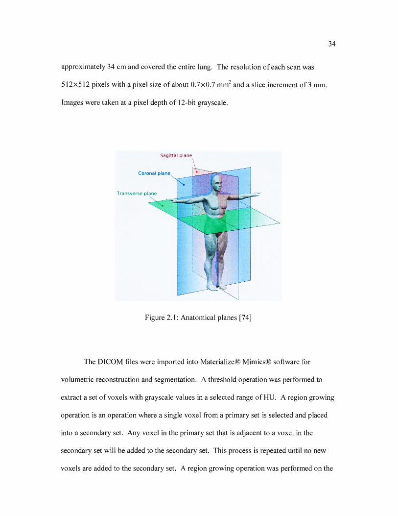
2.1.2. Geometry Creation. CT scans will produce data that represents the
topology of a three dimensional space. The data is presented as a set of two dimensional
slices in the patient's axial (transverse) planes (refer to Figure 2.1). Each two
dimensional slice is a set of grayscale values; one for each pixel in the slice. The
grayscale values are measured in Hounsfield units (HU). When represented as a three
dimensional array, the scanned volume is broken into cells called voxels, each having a
dimension of pixel size x pixel size x slice increment. This data was stored as DI COM
(Digital Imaging and Communications in Medicine) files. The geometry creation process
involves three major steps: (a) volumetric reconstruction, (b) segmentation, and (c)
geometry cleanup. Volumetric reconstruction involves lining up the two dimensional
scan planes on top of each other to create the volume ofvoxels and selecting a set of
voxels based on grayscale values that are likely to contain a target material.
Segmentation involves cutting voxels from the set ofvoxels produced from volumetric
reconstruction that are not contiguous or that do not actually contain the targeted
material. This step relies on intuition and is generally performed manually. Geometry
cleanup is the process of removing defects in the reconstructed model due to the
representation of the geometry by voxels (blocks) and the adjustment of surface
geometries to allow implementation of boundary conditions.
For the current investigation, CT scans were taken of a 57 year old, male, patient
undergoing mechanical ventilation treatment at the University of Missouri at Kansas City
(UMKC) hospital, using a Siemens SOMATOM Definition AS 128 slice CT scanner.
There are several metrics that determine the quality of a CT scan such as: field of view,
resolution, pixel size, slice increment, and pixel depth. The field of view was
approximately 34 cm and covered the entire lung. The resolution of each scan was
512x512 pixels with a pixel size of about 0.7x0.7 mm2 and a slice increment of3 mm.
Images were taken at a pixel depth of 12-bit grayscale.
Sagittal plane
Figure 2.1: Anatomical planes (74]
34
The DICOM files were imported into Materialize® Mimics® software for
volumetric reconstruction and segmentation. A threshold operation was performed to
extract a set of voxels with grayscale values in a selected range of HU. A region growing
operation is an operation where a single voxel from a primary set is selected and placed
into a secondary set. Any voxel in the primary set that is adjacent to a voxel in the
secondary set will be added to the secondary set. This process is repeated until no new
voxels are added to the secondary set. A region growing operation was performed on the

35
set of voxels that had undergone the threshold operation to obtain a continuous set of
voxels. The "calculate 30" operation in Mimics® was used to reconstruct a continuous
volume of air within the lungs.
Figure 2.2 shows a screenshot from Mimics® software. The upper right view
shows a slice of the axial plane (the plane in which the CT scans were taken) where the
main bronchi can be seen. The upper left view shows a slice in the coronal plane which
is constructed by Mimics® from the data in the axial slices. The coronal view has. a clear
image of the first bifurcation. The bottom left view is a slice in the sagittal plane which
was also constructed by Mimics® from the data in the axial slices. In the sagittal view
the trachea can be seen as well as an edge of the endotracheal tube. There are two active
masks shown in the CT scan views. The green mask is the initial thresholding region.
The yellow mask is what was generated after the first region growing operation. The
bottom right view shows the three dimensional reconstructed volume after the first region
growing operation.
The data acquired by the CT scan process represents a measurement of average
attenuation coefficient for X-rays over the voxel volume. In general each type of tissue
will have a small, distinctive range of HU values. Ideally a voxel would only contain one
type of tissue. However, the degree of resolution for this to occur is not attainable with
current imaging techniques. For this reason a voxel that is mostly air may fall within the
threshold range. Towards the lower region of the lungs the airways and alveolar sacs
become so close together that several voxels fall within the threshold region. This means
that a voxel that contains several small airways may be viewed as empty space. This
kind of false positive known as the tissue fraction effect can cause volume leakage for the

36
reconstructed volume and necessitates the segmentation process [7 5]. This volume
leakage can be seen clearly in Figure 2.2.
.. •·
., . •.. )l ~ ·.· .. ..
lil ,~-"""'!:
~ --- r, ot>;,r;:.1 :i ,__. f fil CblKI
'.J f t &ll
J • "'
Figure 2.2: Mask and 30 volume after thresholding and region growing. View from Mimics® software. Upper left: coronal view plane, upper right: axial view plane, lower
left: sagittal view plane, and lower right: 30 view.
Segmentation was performed on the reconstructed volume to remove under-
resolved branches of the lung model. By carefully removing voxels from the mask (a set
of colored pixels displayed in each of the three directional planes in Mimics® software)
of the reconstructed volume the under-resolved regions were essentially cut off of the
tracheobronchial region. A second region growing operation was performed to extract
the rough airways of the computational domain. The extracted (unsmoothed) volume can
be seen in the bottom right view of Figure 2.3 along with its mask in the CT scan views.
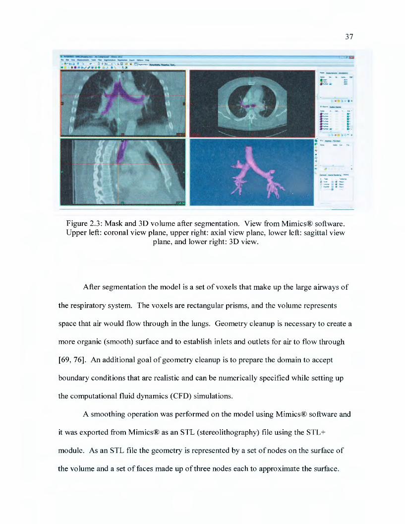
37
)( . . .
• , ,c
.. •. .. •: •..
c.w. ... _ ........... .. '--
·n ....
~ ""'- '"" ::a.? :Jc-:r.r sa ~ .J~ >..•
•
Figure 2.3: Mask and 30 volume after segmentation. View from Mimics® software. Upper left: coronal view plane, upper right: axial view plane, lower left: sagittal view
plane, and lower right: 30 view.
After segmentation the model is a set of voxels that make up the large airways of
the respiratory system. The voxels are rectangular prisms, and the volume represents
space that air would flow through in the lungs. Geometry cleanup is necessary to create a
more organic (smooth) surface and to establish inlets and outlets for air to flow through
[69, 76]. An additional goal of geometry cleanup is to prepare the domain to accept
boundary conditions that are realistic and can be numerically specified while setting up
the computational fluid dynamics (CFO) simulations.
A smoothing operation was performed on the model using Mimics® software and
it was exported from Mimics® as an STL (stereolithography) file using the STL+
module~ As an STL file the geometry is represented by a set of nodes on the surface of
the volume and a set of faces made up of three nodes each to approximate the surface.

38
The STL file was imported into Blender® 2.5 and further smoothing was performed. A
set of faces were selected for each outlet and were projected onto a plane at the end of the
airway perpendicular to the airway the outlet belonged to. To ensure appropriate outlet
conditions extensions were added to each outlet. An extension was created at each outlet
by extruding the projected faces parallel to the airway and gradually transitioning the
airway shape to a circle. A similar process was performed at the inlet of the endotracheal
tube to ensure an appropriate inlet condition. The finished geometry was exported from
Blender® as an STL file. The completed geometry, after smoothing, adding extensions,
and defining the openings for the inlet and outlets is shown in Figure 2.4.
Front View Back View
37 37
Figure 2.4: Completed geometry with extensions. Exported from Blender® 2.5.
39
2.1.3. Geometric Features Present in the Current Model. For CFD simulation
purposes, important features of lung geometry are those that would cause changes in the
fluid flow solution. Obvious examples may be main airway structures such as the nasal
or oral passages, the trachea, or the generations of the lung. The way that these features
are modeled is also important. Various simplifications to the airways have been used in
the past [23, 26, 77-81]. One less obvious feature is the larynx, which a great deal of
study has been devoted to. To summarize the general findings, the larynx creates a jet of
air during inhalation that creates turbulence in the trachea and contributes to turbulent
dispersion and deposition of aerosols in the trachea and upper bronchi [30, 82-85]. Other
less obvious characteristics are the shape and orientation of the airways, which includes
the direction the branching occurs, the branching angles, and any curvature of the
airways. Cartilaginous rings have been given some attention as a potential influence on
fluid flow and particle deposition [33, 68, 86-87]. Studies have also focused on carinal
ridges and tumors [88-91].
In addition to the features of the lung geometry there are features of the ventilator
circuit. The endotracheal tube (ETT) is certainly one of the most important ventilator
circuit features to be included in the model. The endotracheal tube has had some study
devoted to it in the past [68, 92-95]. The focus of these studies has typically been on
measuring the effect of the ETT tube on airway resistance and workload, and hospital
practices to prevent poor placement of the ETT during intubation. However the influence
of the endotracheal tube has yet to be thoroughly explored from a fluid flow perspective,
i.e., studies have not focused on what effects the ETT has on turbulence, flow
distributions, or particle dispersion and deposition.

40
The model used in this study includes the trachea, the left and right main bronchi,
and four to seven generations. There are a total of 41 outlets in the current geometry.
The generation number at the outlets ranges from G4 to G7. Due to the nature of the
reconstruction technique the lengths, sizes, branching angles, branch orientations, and
shapes of the airways are consistent with the actual geometry of the patient. From the
ventilator circuit, the endotracheal tube has been included and the fluid flow from the
ventilator into the endotracheal tube has been modeled with an inlet condition. The
larynx is not present in the current model. However, since the outlet of the endotracheal
tube into the trachea is below the larynx, we hypothesize that the larynx should not have
any significant effect on the fluid flow into the domain. Cartilaginous rings were not
evident in the CT scans and were not included in the current airway model.
2.1.4. Advantages and Potential Problems. Due to the complex nature of the
human airways and the need for accurate modeling, CT scan geometries offer several
distinct advantages. However, there are also ways in which the data collection and
geometry creation processes can contribute to errors in the study. The choice of
geometry modeling technique also depends largely on the degree to which a single set of
airways are representative of any set of airways. This has been looked at, but it is still yet
to be fully determined [28].
Obvious advantages ofusing CT scan based geometries are the more accurate
representation of a patient's airway size, shape, position, curvature, and diameter
variations. CT scans will also capture patient specific characteristics like physical
markers of disease, such as, tumors, or airway constrictions. Other patient specific
characteristics such as lung injuries or surgical procedures or scarring may also be

41
visible. Currently the geometry creation process can be rather lengthy. However, with
advancements in medicalimaging technology and geometry creation software, the speed
at which a computational geometry can be created may surpass the creation time for some
idealized models that include some degree of patient specificity.
Although many aspects of a patient's actual lung geometry can be captured by the
CT scans and are able to be reconstructed, others may be left out. There are some
features of the lung that are known to exist and can be modeled but are not easily
captured or reconstructed. One example of this is cartilaginous rings, which have been
included in studies already mentioned but are not visible in CT scan geometries.
The reasons for the lack of some details in CT scan based geometries can be
linked to several potential factors. The resolution of a scan can cause problems with the
tissue fraction effect and characteristics smaller than a voxel size. Poor resolution can
also lead to a tendency to over-smooth the surfaces. The smoothing operation can cause
sharp features to be dulled or distorted. Cardiovascular and reparatory motion during the
CT scan process can-also lead to a blurring effect that will degrade the resolution in some
parts of the CT scans.
The segmentation process is another source of potential geometric discrepancies.
All of the CT scan quality issues mentioned above can make the segmentation process
more difficult. The segmentation process is performed manually because there is no
readily available software for automatic human airway segmentation, and if such
software did exist, it would be unlikely that it could mimic the human intuition and
knowledge of the human airways. Because segmentation is performed manually it could
42
contribute significantly to geometric discrepancies if it were performed by someone who
is unfamiliar with the structure of the human airways.
2.1.5. Geometry Statistics. Geometric characteristics of the current airway
model are given in Table 2.1. The outlet numbers provided in Table 2.1 correspond to
the labels shown in Figure 2.4. The generation column designates how far down the
tracheobronchial tree the outlets occur, with the trachea being GO and the main bronchi as
G 1 and so forth. The size of the airways is given as hydraulic diameter described in
Equation 1.1. The flow ratios are provided for each outlet as a percentage of the mass
flow rate at the endotracheal tube. These flow ratios will be discussed further in § 3.3.3.
The geometric features present in the model down to the third generation have
been compared to the two most common statistical models in Table 2.2. It is difficult to
compare airway size directly with the statistical models because the size of human
airways varies based on height, weight, physical activity, age, gender and several other
physiological factors. For this reason the airway sizes of the current model and the
statistical models were non-dimensionalized by defining a diameter ratio for each
bifurcation. The diameter ratio presented in the table is defined as the daughter branch
diameter divided by the parent branch diameter. The smaller diameter ratio for each
bifurcation was designated as the minor diameter ratio and the larger was designated as
the major diameter ratio. For the most part the diameter ratios are consistent with those
presented in the Weibel and Horsfield models.
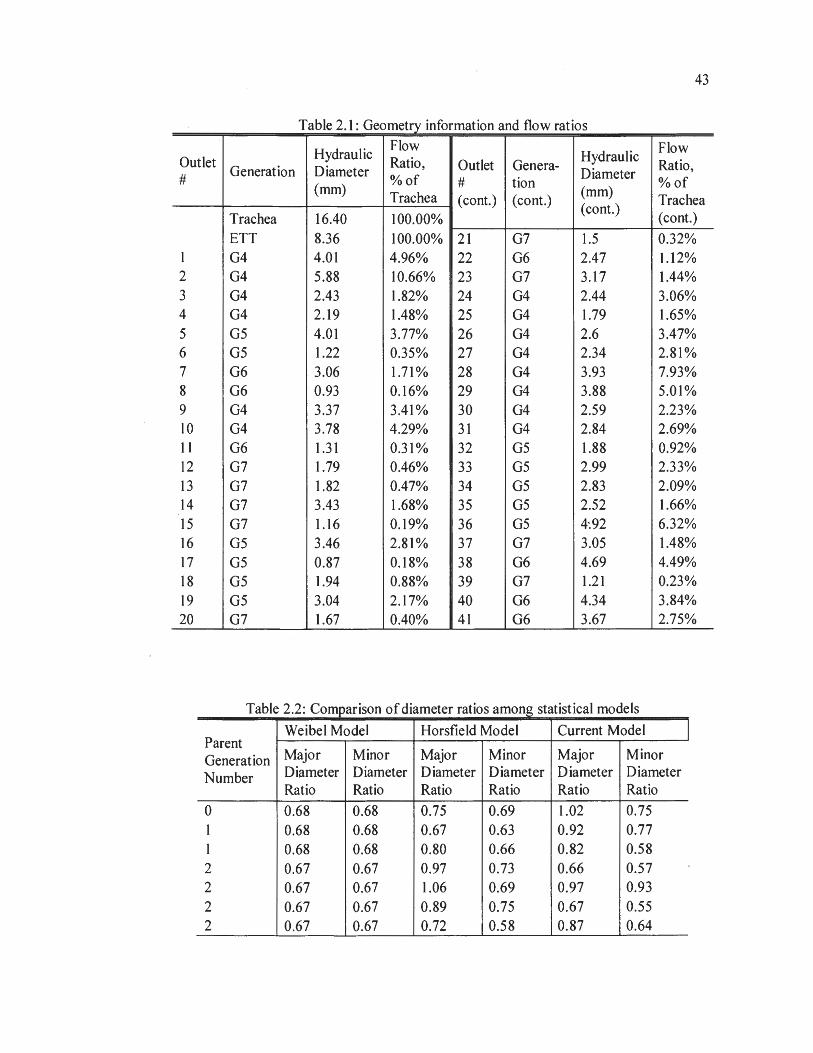
43
Table 2.1: Geometry information and flow ratios
Hydraulic Flow Flow
Outlet Ratio, Outlet Genera-Hydraulic
Ratio, Generation Diameter Diameter # (mm)
%of # tion %of Trachea (cont.) (cont.)
(mm) Trachea
Trachea 16.40 100.00% (cont.)
(cont.)
ETT 8.36 100.00% 21 07 1.5 0.32% 1 04 4.01 4.96% 22 06 2.47 1.12% 2 04 5.88 10.66% 23 07 3.17 1.44% 3 04 2.43 1.82% 24 04 2.44 3.06% 4 04 2.19 1.48% 25 04 1.79 1.65% 5 GS 4.01 3.77% 26 04 2.6 3.47% 6 GS 1.22 0.35% 27 04 2.34 2.81% 7 06 3.06 1.71% 28 04 3.93 7.93% 8 06 0.93 0.16% 29 04 3.88 5.01% 9 04 3.37 3.41% 30 04 2.59 2.23% 10 04 3.78 4.29% 31 04 2.84 2.69% 11 06 1.31 0.31% 32 GS 1.88 0.92% 12 07 1.79 0.46% 33 GS 2.99 2.33% 13 07 1.82 0.47% 34 GS 2.83 2.09% 14 07 3.43 1.68% 35 GS 2.52 1.66% 15 07 1.16 0.19% 36 GS 4:92 6.32% 16 GS 3.46 2.81% 37 07 3.05 1.48% 17 GS 0.87 0.18% 38 06 4.69 4.49% 18 GS 1.94 0.88% 39 07 1.21 0.23% 19 GS 3.04 2.17% 40 06 4.34 3.84% 20 07 1.67 0.40% 41 06 3.67 2.75%
T bl 2 2 C a e .. ompanson o fd' .. 1 d I iameter ratios among stat1st1ca mo es
Weibel Model Horsfield Model Current Model I Parent Generation Major Minor Major Minor Major Minor
Number Diameter Diameter Diameter Diameter Diameter Diameter Ratio Ratio Ratio Ratio Ratio Ratio
0 0.68 0.68 0.75 0.69 1.02 0.75 1 0.68 0.68 0.67 0.63 0.92 0.77 1 0.68 0.68 0.80 0.66 0.82 0.58 2 0.67 0.67 0.97 0.73 0.66 0.57 2 0.67 0.67 1.06 0.69 0.97 0.93 2 0.67 0.67 0.89 0.75 0.67 0.55 2 0.67 0.67 0.72 0.58 0.87 0.64
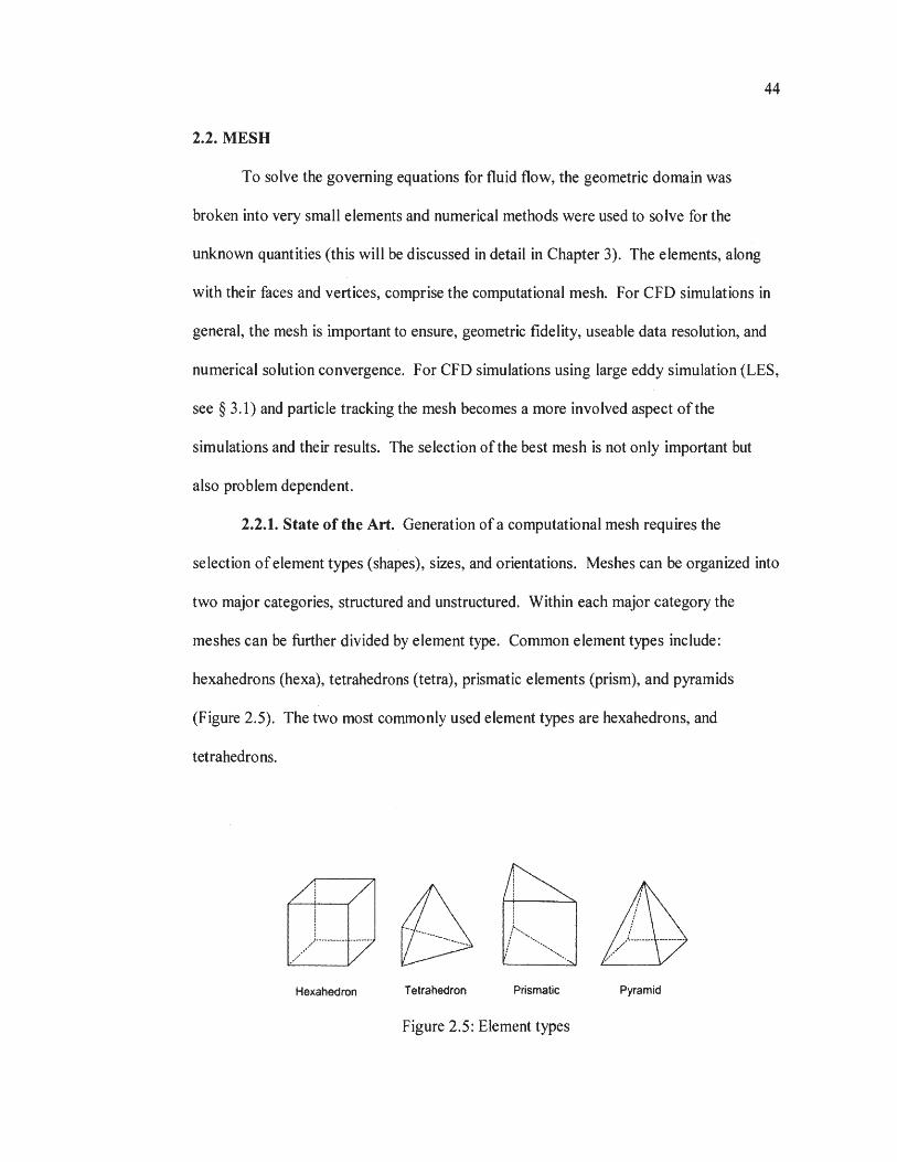
44
2.2. MESH
To solve the governing equations for fluid flow, the geometric domain was
broken into very small elements and numerical methods were used to solve for the
unknown quantities (this will be discussed in detail in Chapter 3). The elements, along
with their faces and vertices, comprise the computational mesh. For CFD simulations in
general, the mesh is important to ensure, geometric fidelity, useable data resolution, and
numerical solution convergence. For CFD simulations using large eddy simulation (LES,
see § 3.1) and particle tracking the mesh becomes a more involved aspect of the
simulations and their results. The selection of the best mesh is not only important but
also problem dependent.
2.2.1. State of the Art. Generation of a computational mesh requires the
selection of element types (shapes), sizes, and orientations. Meshes can be organized into
two major categories, structured and unstructured. Within each major category the
meshes can be further divided by element type. Common element types include:
hexahedrons (hexa), tetrahedrons (tetra), prismatic elements (prism), and pyramids
(Figure 2.5). The two most commonly used element types are hexahedrons, and
tetrahedrons.
@~ I
. -- ·········-......... .
Hexahedron Tetrahedron Prismatic Pyramid
Figure 2.5: Element types
45
Due to the problem specific nature of mesh selection there have been studies of
mesh type for cases related to the present case [96-97]. These studies do suggest a
preference towards hexahedral elements that are aligned with direction of the flow.
However they were performed with a RANS model on an idealized double-bifurcation.
In addition Vinchurkar [97] suggests that structured hexahedral meshes are often
prohibitively expensive in terms of time, despite the high quality solutions they typically
produce. Even within the specific field of human airway fluid mechanics there is a
variety of mesh styles being used for different problem formulations. Table 2.3 gives a
summary of some studies and the mesh styles they have used. In general, the geometry
and turbulence modeling formulation governs what type of mesh is fit to the geometry.
Meshes for CT scan based geometries are almost always unstructured and invo Ive
tetrahedrons. Unstructured hybrid meshes with tetrahedrons in the center and prism
layers near the wall are frequently used with the low Reyno Ids number (LRN)
formulation of the k-w model. Prism layers are rarely used in conjunction with LES due
to the cell anisotropy. For an idealized geometry hexahedrons are sometimes used but
generally in cases where there are few generations.

46
T bl 2 3 L' f b I a e .. 1terature review o tur u ence mo d I' e mgan d mes h sty es
Author Modeling and (year) conditions Geometry Mesh type Lambert A.R. et al LES, steady (2011)[31] inlet velocity CT-scan based, mouth up to G7 Tetrahedral · Xia, G. et al LES, Sinusoidal CT-scan based, single bifurcation (2010)f181 inlet waveform G3 to G4 Tetrahedral Choi,J. et al LES, Sinusoidal (2010)[71] inlet waveform CT-scan based, mouth up to G7 Tetrahedral
CT-scan based, Two models start Lin, Ching- from trachea up to G6: Long, et al DNS, steady Model 1- includes mouth and larynx (2007) [83] inlet velocity Model 2- without mouth and larynx Tetrahedral
Realistic model: hybrid: tetrahedral with prism layers
LRN k-w, Ideal model: Xi, J. et al steady inlet Mouth to trachea, CT -scan based structured (2008) [99] velocity and idealized hexahedral
LRN k-w, Hybrid: Xi, J. et al steady inlet tetrahedral with (2008) [30] velocity CT-scan based larynx up to GS prism layers Isaacs, K.K. et al (2006) laminar, steady Structured [100] inlet velocity Idealized model, single bifurcation hexahedral Zhang, Z. et LRN k-w, al (2008) steady inlet Idealized geometry, series of triple Structured r 1o11 velocity bifurcations to simulate GO-G 15 hexahedral Farkas, A. et Laminar al steady inlet Idealized geometry. Trachea up to (2007) [ 102] velocity G2 tetrahedral
2.2.2. Mesh Creation. The mesh selection problem was carefully considered for
this study. Structured hexahedral meshes have proven to be a good choice for geometries
with simple features such as circular airways, symmetrical branching patterns, or a low
number of bifurcations. The geometry of the current study is based off of CT scans and

is complex for meshing purposes. A structured hexahedral mesh was attempted in
ANSYS® ICEM® CFD but found to be prohibitively time consuming and it was not
clear that a grid absent of rapid changes in cell size would be achievable.
47
An unstructured hexahedral mesh created by a body fitted Cartesian method was
also considered but a mesh with isotropic and high quality elements was not able to be
realized. The modeling guide for the chosen solver, CFX®-13.0, suggests the use of
isotropic grids with tetrahedral rather than hexahedral elements [98]. ANSYS® ICEM®
CFD also offered options for hybrid meshes such as a tetrahedral mesh with prism layers
in the near wall region or a tetrahedral mesh with a hexahedron core. However the cells
of a prism layer would be anisotropic and a hexahedron core would require a sudden
change in element type and size. For these reasons a fully tetrahedral mesh was adopted
for the current study.
The computational mesh was created using ANSYS® ICEM® CFD. The
geometry was imported as an STL file after geometry cleanup and the addition of
extensions in Blender® 2.5. A build topology operation was performed to establish the
curves and points from the edges of the surfaces and to ensure there were no holes or
gaps in the geometry. The surfaces of the geometry were separated into several different
parts so that mesh parameters could be specifically set for each part. Curves and points
that were not meant to guide the mesh were deleted to avoid unnecessary constraints for ·
the mesh. Parameters including maximum element size and tetra size ratio were set for
each part. The smoothing option was turned off so that the surface mesh could be later
smoothed without the volume elements to constrain it.
48
An octree method was used to compute a mesh in the domain [103]. Octree
meshing is performed by continually dividing a tetrahedron that encloses the entire
domain. When an element is below the maximum element size it will stop splitting.
Then if an element is intersected by a surface then the mesher will look at the distance
between the nodes of the element and the surfaces. If the node is within a tolerance then
the node is projected to the surface. If the node is not within the tolerance then the
element is refined. In this way the mesher will create a mostly uniform mesh that is·fit to
the surface of the geometry. For the current study the mesh generated in the volume was
not the focus of this operation. The octree method created a reasonable surface mesh but
the volume could better be created with an operation that grows mesh inward from the
surface mesh.
The volume elements were then deleted while the surface elements were retained
for smoothing. To obtain a high quality surface mesh the surface elements were
smoothed first using a Laplace smoothing operation. The goal of this operation is to find
a good center point for each node with respect to the nodes it is connected to by edges.
This smoothing process is iterative and will result in a more uniform spacing of nodes.
After the Laplace smoothing operation a smoothing operation was performed without the
Laplace smoother. This operation focused on moving nodes to improve the quality of the
surface elements. This smoothing operation is also iterative and resulted in a high quality
surface mesh. It is important to note that during the smoothing operations the nodes were
constrained to the surface specified in the input STL file.
The surface elements were then examined for quality. The quality of a surface .
element (triangle) is defined as the minimum ratio of the height of the triangle to its

49
corresponding base length, normalized so that an equilateral triangle would have a quality
of 1. Any element that was of quality less than 0.45 was manually corrected by splitting
a mesh edge or merging two mesh nodes and re-smoothing. The minimum quality of any
surface element was 0.455 and the average quality of surface elements was 0.866. A total
of 2.39x 10⁵ surface elements were created.
To create a high quality volume mesh with a smooth transition in element size, an
advancing front Delaunay method was used [103]. This operation takes the surface·mesh
as an input and will place points in the interior and create a Delaunay triangulation to
determine edges and faces of the created tetrahedral elements. A growth ratio of 1.25
was used to control the expansion of the volume elements as the distance from the wall
increased. After creation of the volume elements a smoothing operation was performed
to improve the quality of the volume elements. Several iterations were first performed
without modifying the surface mesh. Several more iterations were performed while
allowing the surface to adjust along with the volume. The surface nodes were once again
constrained to the surfaces of the geometry.
The volume elements were then examined for quality. Any element that was of
low quality was manually corrected by splitting a mesh edge or merging two mesh nodes
and re-smoothing. The quality of a tetrahedral volume element is defined as the ratio of
the radius of an inscribed sphere to the radius of a circumscribed sphere, normalized so
that a regular tetrahedron would have a quality of 1. The minimum quality of any
volume element was 0.400 and the average quality of the volume elements was 0.746. A
total of 1.11 x I 06 tetrahedral volume elements were created and there were a total of
2.50x 10⁵ nodes in the computational mesh. The created mesh is shown in Figure 2.6.
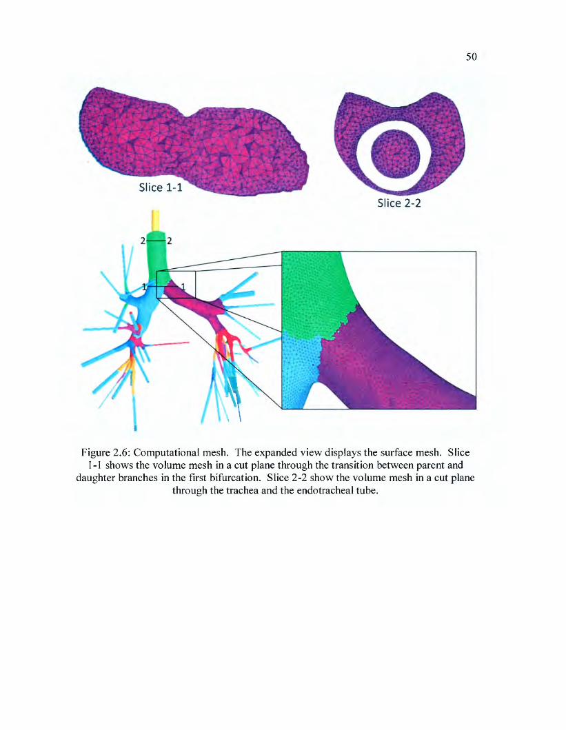
50
Slice 2-2
2 2
Figure 2.6: Computational mesh. The expanded view displays the surface mesh. Slice 1-1 shows the volume mesh in a cut plane through the transition between parent and
daughter branches in the first bifurcation. Slice 2-2 show the volume mesh in a cut plane through the trachea and the endotracheal tube.
51
3. MODELING
This study models fluid flow and particle transport and deposition in a realistic
airway geometry. Computational fluid dynamics (CFD) was employed to solve
governing equations for the flow field variables. CFD is a set of numerical methods used
to model and solve equations that govern fluid motion; most notably the conservation
equations for mass, momentum, and energy [104]. A computational domain with a set of
boundary conditions is divided into many elements in time and space over which, the
modeled equations are applied and solved algebraically to obtain numerical values for
field variables at discrete points [104].
Fluid and particle properties, turbulence modeling, boundary conditions, and
particle transport modeling were carefully chosen and specified in the commercial CFD
software AN SYS® CFX®. Several of the numerical specifications were set using user
FORTRAN subroutines or CFX® expression language (CEL). Simulations were run in
parallel on a machine with 8 Intel® Xeon® E5620 processors (2.4 GHz), 24 GB RAM,
and Windows® 7 Enterprise edition. This chapter will offer detailed descriptions of the
numerical modeling of, momentum, particle transport, and boundary conditions used for
the simulations. The references cited should be consulted for further detail on the
numerical models presented here.
3.1. MOMENTUM .
The working fluid for the simulations run for this study is dry air at 25 °C with a
constant density of p = 1.185 kg/m3 and a dynamic viscosity ofµ= 1.831x10⁻⁵ kg/m·s ~t
an ambient pressure 1 atm. A transient simulation was run for one breathing cycle. Heat
transfer and gravity were not considered in this study.
52
At peak inspiratory velocity the Reynolds number throughout the domain ranges
from about 180 to 13 ,400 indicating that both laminar and turbulent conditions should be
seen in the flow as discussed in§ 1.1. To model turbulence, large eddy simulation (LES)
was used. The wall-adapted local eddy-viscosity (WALE) model was chosen for the
subgrid-scale eddy viscosity model [105]. The ability of LES to resolve large scale
turbulence eddies gives it a distinct advantage over Reynolds averaged Navier-Stokes
(RANS) models for accurately modeling particle transport [106]. The WALE model w-as
chosen for subgrid-scale eddy viscosity modeling for its ability to reproduce the laminar
to turbulent trans it ion process [ 1 0 5].
The principle behind LES is a filtering of the large scale turbulence. The larger
scale flows are directly resolved while the smaller scales are modeled, usually with an
eddy viscosity model [l 07]. Particle motion is influenced more by the larger scales of
fluid motion and the effect of the smaller scale (subgrid scales) turbulent motion is
reduced further in the case of particles with higher inertia [108]. Direct numerical
simulation (DNS) would resolve all of the flow scales, but is computationally expensive
and may not add much due to the dominance of the large scales for particle transport.
The filtered conservation of mass equation for incompressible flow is:
au. 0 -'=
ax; (3.1)
where u; is the ith velocity component with an overbar denoting filtering.
The filtered momentum equation for incompressible flow is [109]:
53
(3.2)
where x; is the /h position component, p is the fluid density, p is the pressure, v is the
fluid kinematic viscosity, and riJ is the subgrid-scale stress defined by [ 109]:
(3.3)
The relationship between the subgrid-scale stress and the large-scale strain rate tensor 8;1
is expressed in Equation 3.4 [109].
(3.4)
The strain rate tensor, 8;1 is defined by [109]:
(3.5)
The subgrid scale viscosity Vsgs for the LES WALE model is modeled by [ 109]:
· (3.6)
In Equation 3.6 s: is the traceless symmetric part of the square of the velocity gradient
tensor i.e. [ 109]:
54
(3.7)
where giJ is the velocity gradient tensor i.e. [I 09]:
(3.8)
A second order central differencing scheme was used for advection and a second order
backwards Euler scheme was used for transience. A residual target of I 0-4 was set for
convergence at each time step. ANSYS® CFX ® is an implicit solver.
3.2. PARTICLE TRACKING
To model particle tracking in the domain, a Lagrangian partic!e tracking method
was used. The particles were assumed to have a low enough volume fraction as to not
have a significant effect on the carrier fluid. The particles used in this study were
assumed to be spherical particles with constant diameters with a constant density of 2000
kg/m3• Particles were injected at the inlet of the domain at random positions given by a
uniform distribution. The diameters of the particles injected were selected from a
uniform distribution between 0.05 and IO µm. The velocity of the particles at the site of
injection was set to match the velocity of the fluid. At the highest volumetric flow rate
seen during inspiration, the Stokes numbers of the particles ranged from 2.90x 10⁻⁵ to
2.95 throughout the domain. A FORTRAN user subroutine was used so that the rate of
particles injected scaled with the inlet mass flow rate such that the total number of
particles would be close to l 00,000.

55
The injected particles were then tracked through the domain until the particle
deposited on the wall, escaped from the domain, or encountered some form of integration
error. Particles were considered to have deposited on the wall when the distance between
the particle center and the wall was less than the particle radius. Upon deposition a user
FORTRAN subroutine was called to output variables including the particle diameter,
position, and time of deposition. These values were used for post processing the particle
deposition results. A particle was considered to have left the domain when the partic-le
crossed an outlet boundary. An integration error would occur when the particle exceeded
the maximum number of integration steps i.e. 1,000,000, when the particle exceeded the
maximum tracking distance i.e. 100 m, or when a particle's velocity became very close to
zero. Particle end statuses will be discussed further in § 4.6.1.
As the particles were tracked through the domain, the particle displacement was
calculated using forward Euler as [109]:
(3.9)
where, Xp is the particle position, v is the particle velocity and l1t is the particle tracking
time step size. The subscript n in Equation 3.9 indicates the particle tracking step
number. The particle velocity v comes from the particle momentum equation [ 109]:
(3.10)

56
where mp is the mass of the particle, and Fall is the sum of all the forces acting on the
particle. The particle momentum equation (Equation 3.10) is a form of the generic
transport equation with an analytic solution. The particle velocity vis solved for by using
the analytic solution. The forces that make up Fall include the drag force Fv, the Saffinan
lift force Fr, and the Brownian motion force FB, as used by Xi et al [30]. These forces
were implemented in ANSYS® CFX® with a user FORTRAN subroutine. The
calculations of these forces are briefly described below. Refer to the cited works for
further detail or derivation of these expressions. The effects of gravity were not
accounted for in this study because the direction of gravity during drug delivery for this
patient was not well known. Particles were tracked over several iterations during each
fluid flow time step. The particle time step was determined by dividing the local element
length scale by the particles velocity and the number of time steps per element, which
was set at I 0.
3.2.1. Drag Force. The drag force is the resistive force of the fluid on the particle
due to their relative velocities. The ;th component of the drag force term Fv is modeled in
this study by:
P11tCDd; I u-v I F.v ·. = (u . -v.) ,, 8C I I
c
(3.11)
where P! is the fluid density, dp is the particle diameter, and u is the fluid velocity. The
expression of Morsi and Alexander was used for drag coefficient of the particle, Cv
[11 O]. In Equation 3.11, the Cunningham correction factor, Cc, is described by [111 ]: ·
57
C, = I+ :. ( 2.34 + l.05e --0,9-'f) (3.12)
where Ji. is the mean free path, taken to be 65 nm. The Cunningham correction factor is
on the order of 1.15 for a 1 µm diameter particle and this will increase rapidly as the
particle size decreases, but is negligible for particle larger than a 10 µmin diameter [111].
In this study the Cunningham correction factor is expected to be significant for the
particle diameter range of0.05-10 µm.
3.2.2. Lift Force. The lift force is caused by a pressure differential that occurs
under the conditions of a particle moving at a different speed than the fluid at a location
where a large velocity gradient is present such near a wall [58]. A particle that is moving
faster than the fluid will be forced towards the wall, while a particle moving slower than
the fluid will be forced away from the wall [58]. The drag force will ac_t to diminish the
difference in particle and fluid speeds, but for particles with significant inertia in areas
with rapidly changing geometry or significant turbulence, this force is expected to play a
large role in the particle's motion. The ith component of the lift force FL is described by
[ 112]:
d 2" -pf pl1;[ 2 J FL i = us . g(K,A)
· 4m p
(3.13)
where n is the unit wall normal vector pointing out of the domain. The wall-tangerit slip
velocity Us in Equation 3.13 is described by [112]:
u =v ·t-u ·n s (3.14)
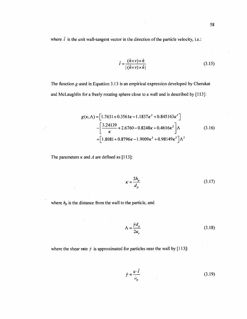
58
where i is the unit wall-tangent vector in the direction of the particle velocity, i.e.:
" (nxv)xn t=----
l(nxv)xnl (3.15)
The function g used in Equation 3.13 is an empirical expression developed by Cherukat
and McLaughlin for a freely rotating sphere close to a wall and is described by [113]:
g(K,A) = [ 1.7631 +0.3561K-l.1837K2 +0.845163K3 J -[
3·2:
39 +2.6760-0.8248K-0.4616K2 ]A (3.16)
+[ 1.8081 + 0.8796K-l.9009K2 +0.98149K3]A2
The parameters K and A are defined as [ 113]:
where hp is the distance from the wall to the particle, and
fdp A=-
2us
where the shear rate y is approximated for particles near the wall by [113]:
" . u ·t r~--rip
(3.17)
(3.18)
(3.19)

59
3.2.3. Brownian Motion Force. The Brownian motion force is caused by
random bombardment of the aerosol particle by the surrounding gas particles [111]. At a
microscopic level the effect of the force is random in direction, however at a macroscopic
level the particles begin to move from areas of higher concentration to lower
concentration and this effect is often referred to as particle diffusion [ 111]. The effects of
Brownian forces are most noticeable on particles that have very low inertia i.e. particles
with a diameter less than 1 µm [114]. The ith component of the Brownian motion force,
(3.20)
where k8 is the Boltzman constant, Tis the absolute temperature of the-fluid, L1t is the
particle integration time step, and ( is a vector of 3 randomly generated numbers each
taken from a Gaussian distribution with zero mean and unit variance. The Brownian
diffusivity b in Equ_ation 3.20 is defined as:
- k .TC D=-o __ c 31tµaP
(3.21)
where µ is the dynamic viscosity of the fluid.
3.3. BOUNDARY AND INITIAL CONDITIONS
Boundary conditions were carefully selected and implemented for the inlet, the ·
walls of the CT scanned reconstructed geometry, the walls of the artificial extensions
60
added to the outlets, and the outlets of the computational domain. This section discusses
the numerical specifications at the inlet, walls, and outlets of the domain and the initial
conditions.
3.3.1. Inlet. The inlet refers to the circular boundary at the top of the
endotracheal tube which is technically only an inlet during inspiration. The velocity at
the inlet was specified with Cartesian velocity components. In the domain creation
process an extension was added to the inlet reconstructed from the CT scans so that there
was a smooth transition to a circular cross section. In addition the domain was oriented
so that the plane of the inlet coincided with the x-y plane and the center of the circular
inlet was coincident with the origin. These adjustments facilitated the implementation of
a Cartesian velocity component specification at the inlet. The velocity profile at the inlet
was specified as a fully developed turbulent velocity profile described by [30]:
(R rJt u(r,t) = 1.224um(t) R (3.22)
where r is the radial distance from the origin, R is the radius of the inlet, and Um is the
time varying mean velocity at the inlet, which is dependent upon the inspiratory
waveform. The selection of this profile is appropriate considering the turbulent Reynolds
numbers present in the tube over most of the breathing cycle. Curvature effects in the
tube upstream of the inlet were not considered for this study.
3.3.2. Walls. The walls of the domain were assumed to be smooth and rigid. A
no slip boundary condition was applied to the walls of the domain i.e. the velocity was
zero at the walls. The effects of the mucus layer lining the walls were not accounted for

61
in this study. The surface at the top of the trachea connecting the endotracheal tube and
the walls of the trachea is due to the end of the CT scan field of view. This area is not
physiologically realistic but was modeled just as the other walls in the domain. In reality
the flow across this area is expected to be small because of the balloon attached to the
endotracheal tube designed to seal the endotracheal tube against the walls of the larynx.
The walls that were reconstructed from CT scans were set with parallel and perpendicular
restitution coefficients of zero so that particles would deposit on contact. The walls of
the artificial extensions at the outlets were given a parallel restitution coefficient of 1.0
and a perpendicular restitution coefficient ofO. l so that no particles would collect on
those walls.
3.3.3. Outlets. The flow at the outlets was specified with a mass flow rate. The
mass flow rates were given as fractions of the instantaneous mass flow rate at the inlet of
the domain. Similar mass flow rate specifications have been used past studies [JO, 70,
115-116]. The mass flow rate fraction at each of the outlets was calculated based on data
from Horsfield et al [8]. The mass flow rate fraction Fm at the /h outlet is:
F . = F . 411,; m,1 H ,J L1
LicJ?s,j
(3.23)
where F H.J is the mass flow rate fraction for the l branch given by Horsfield et al, AG7.i is
the 07 equivalent area of the /h outlet i.e.:
(3.24)

· where Rpd is the parent -daughter diameter ratio, taken here as 1.25 (the average of the
parent daughter diameter ratios for generations G4-G7 in Weibel's model A) [17}. In
Equation 3.23, AG7sJ is defined as the sum of the G7 equivalent areas of the outlets that
are supplied by the branch corresponding to the/ branch given by Horsfield et al [8].
The mass flow rates at the outlets are specified, however, the distribution of the mass
flow over the outlet is a function of the mass flow just upstream of the outlet [98].
62
3.3.4. Initial Conditions. Time t=O is set to be the onset of inspiration and it is
assumed that an identical breathing cycle has just finished. For all waveforms except the
pressure controlled sinusoidal waveform, (which will be discussed in§ 4.1) the flow in
expiration is quick at the beginning of expiration and then flattens out asymptotically
approaching zero. The inlet flow rate in expiration is less than 2 % of the maximum inlet
flow rate in expiration for t > --3.2 s. Therefore at time t=O the velocity was set as zero.
63
4. RESULTS AND DISCUSSION
To simulate realistic ventilator condition th~ respiratory waveforms were
modeled. Mean flow speed at the inlet was set to reproduce respiratory waveforms used
by commercial ventilators. To establish confidence in the computational model grid
convergence and time step convergence studies were performed. A validation study was
also performed to check the computational model against experiments [117]. When these
studies were completed simulations were ran using the various waveforms discussed in §
4.1. In this section, we discuss respiratory waveform creation, grid convergence, time
step convergence, and validation studies, as well as fluid flow and particle tracking
results obtained using numerical simulations.
4.1. WAVEFORMS
In this study seven different waveforms were created and modeled in the inlet
condition. The waveforms represent a number of ventilator conditions commonly seen in
manufactured mechanical ventilators [ 47]. This section will describe the creation of the
respiratory waveforms and the application of those waveforms to the computational
model.
The waveforms created for this study were governed by the equations of motion
for the lungs given in Equation 1.3 and Equation 1.4 in § 1.3 .2. One of the three control
variables (pressure, volume, or flow rate) was constrained and the other two were solved
for numerically. Waveforms were constrained to have the same tidal volume and period.
A small rise/fall time was incorporated to smooth the waveforms and to avoid non
physical flow phenomena such as an instantaneous (step) change in flow velocity. The
tidal volume of the lung was approximated as 650 mL and the lung properties of

.64
compliance and resistance (Equation 1.5 and Equation 1.6 respectively) were taken as
0.127 Liem H20 and 4.33cm H20/(L/s) respectively. The values for resistance and
compliance were found by averaging the resistances and compliances reported by
Grimby for patients with COPD [118]. The ventilator waveforms used in this study are
shown in Figure 4.1.
12
10
q, 8 J:
1 6
!!? 4 :::, UI
! Cl.
-2 0
700
600
500 :J' g 400
~ 300 :::,
J 200
100
100
80
60
c 40
£ 20
1 0
u. -20
-40
~
-80 0
Pressure Waveforms
2 Time(s)
.... ........
Volume Waveforms
~--- .......... ,, ........ ;' '
............
"' ' , '
2
Time(s)
Flow Waveforms
' '
- ____ ..,,
' .............
Pressure Control: Constant Pressure Control: Exponential Pressure Control: Sinusoidal
2 Time(s)
------· Volume Control: R•mp • • • • • • • • • • • • • • • Volume Control: Sigmoid -·-·-·-· Flow Control: Ascending Ramp - .. - .. _.. Flow Control: Descending Ramp
Figure 4.1 : Ventilator waveforms

65
Seven waveforms, commonly used by commercial ventilators, are shown in
Figure 4.1. The waveforms represent three different methods of controlling how ~ patient
respires. Three of the waveforms would be seen for a ventilator that is controlling
breaths by the ventilator output pressure (pressure control). Two of the waveforms would
be seen-for a ventilator that is controlling breaths by monitoring the volume of air that has
passed into the lung (volume control). The remaining two waveforms would be seen for
a ventilator controlling the flow rate into the lungs (flow control). The sinusoidal
pressure waveform would be seen with the use of a reciprocating pump and this is the
reason why the shape of the curve is slightly different from the rest. For all waveforms
except for the sinusoidal pressure waveform the inspiration time was set to approximately
1 second. The expiration is in the shape of an exponential decay, modeling a natural
outward breath based on the elasticity of the lung.
MATLAB® scripts were created to generate the waveforms. Simple shapes,
including ramps, sinusoids, and an exponential rise, were imposed on the control
variables during inspiration as seen used by commercial ventilators [47]. In all
waveforms except the pressure controlled sinusoidal waveform, the expiration was
obtained by setting the pressure to zero. For the pressure controlled ventilation mode the
pressure was set throughout the breathing cycle, the volume waveform was solved for by
applying a 4th order Runga-Kutta method to the equation of motion for lungs (Equation
1.3), and the flow waveform was solved for by plugging in the values for pressure and the
solved values for volume into the equation of motion for lungs. The volume is assumed
to be zero as an initial condition. For the volume controlled ventilation mode the volume
was initially set for inspiration, the flow waveform was solved for by numerically

66
·integrating the volume waveform by trapezoid rule, a small rise/fall time was
incorporated to smooth the flow waveforms and to avoid non-physical flow phenomena
such as an instantaneous (step) change in flow velocity, the volume waveform was re
solved for from this new flow waveform using finite difference, and the pressure was
solved for by plugging in the values for volume and flow into the equation of motion for
lungs. For the flow controlled ventilation mode the flow was set for inspiration, the
volume waveform was solved for by applying finite difference to flow waveform, and the
pressure was solved for by plugging in the values for volume and flow into the equation
of motion for lungs. The volume and flow waveforms in expiration for volume and flow
ventilation modes were solved for by the method applied for the pressure controlled
mode. The tidal volume was set for the final waveforms by iteratively scaling the input
waveforms for the control variables and measuring the resulting tidal volume. The
averaged velocity across the inlet was calculated from the flow rate waveform using the
area of the inlet and was output to a file for use in ANSYS® CFX®. The MATLAB®
scripts are provided in APPENDIX C.
4.2. GRID CONVERGENCE
A study was performed to ensure that the solution obtained would be grid
independent, The grid convergence study was carried out on a simplified geometry
described by Zhao and Lieber [119] which also allowed us to compare our preliminary
simulations with experimental data obtained from their work. In this study the parent
tube diameter, D, is taken to be the same as the hydraulic diameter of the trachea of the
CT scan model geometry, i.e. 16.4 mm. The geometrical feature relationships of the
model bifurcation to the parent diameter are taken to be the same as in Zhao's geometry
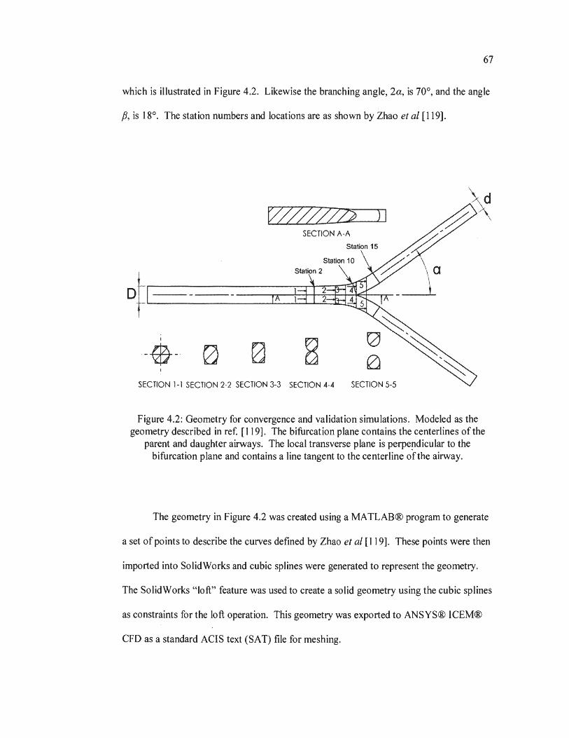
67
which is illustrated in Figure 4.2. Likewise the branching angle, 2a, is 70°, and the angle
/J, is 18°. The station numbers and locations are as shown by Zhao et al [119].
' O
\ I
-0- 0 SECTION 1-1 SECTION 2-2 SECTION 3-3 SECTION 4-4 SECTION 5-5
Figure 4.2: Geometry for convergence and validation simulations. Modeled as the geometry described in ref. [119]. The bifurcation plane contains the centerlines of the
parent and daughter airways. The local transverse plane is perpe!'}dicular to the bifurcation plane and contains a line tangent to the centerline of the airway.
The geometry in Figure 4.2 was created using a MATLAB® program to generate
a set of points to describe the curves defined by Zhao et al [119]. These points were then
imported into SolidWorks and cubic splines were generated to represent the geometry.
The SolidWorks "loft" feature was used to create a solid geometry using the cubic splines
as constraints for the loft operation. This geometry was exported to ANSYS® ICEM®
CFD as a standard ACIS text (SAT) file for meshing.
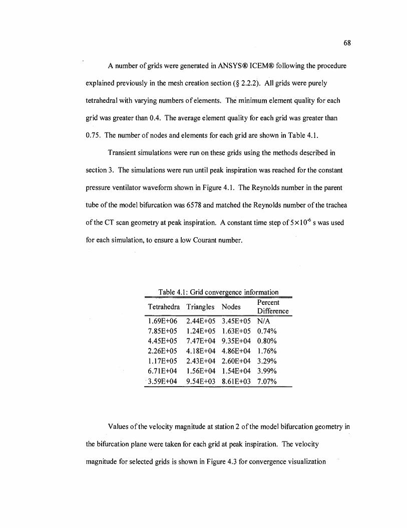
68
A number of grids were generated in ANSYS® ICEM® following the procedure
explained previously in the mesh creation section(§ 2.2.2). All grids were purely
tetrahedral with varying numbers of elements. The minimum element quality for each
grid was greater than 0.4. The average element quality for each grid was greater than
0.75. The number of nodes and elements for each grid are shown in Table 4.1.
Transient simulations were run on these grids using the methods described in
section 3. The simulations were run until peak inspiration was reached for the constant
pressure ventilator waveform shown in Figure 4.1. The Reynolds number in the parent
tube of the model bifurcation was 6578 and matched the Reynolds number of the trachea
of the CT scan geometry at peak inspiration. A constant time step of 5 x 10⁻⁶ s was used
for each simulation, to ensure a low Courant number.
Table 4.1: Grid convergence information
Tetrahedra Triangles Nodes Percent Difference
1.69E+06 2.44E+05 3.45E+05 NIA 7.85E+05 1.24E+05 1.63E+05 0.74% 4.45E+05 7.47E+04 9.35E+04 0.80%
2.26E+05 4.18E+04 4.86E+04 1.76%
l.17E+05 2.43E+04 2.60E+04 3.29% 6.71E+04 l .56E+04 1.54E+04 3.99%
· 3.59E+04 9.54E+03 8.61E+03 7.07%
Values of the velocity magnitude at station 2 of the model bifurcation geometry in
the bifurcation plane ~ere taken for each grid at peak inspiration. The velocity
magnitude for selected grids is shown in Figure 4.3 for convergence visualization
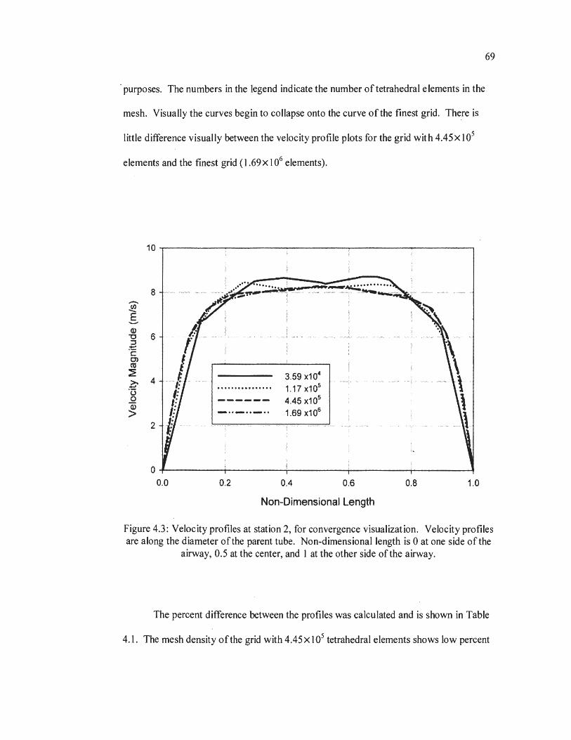
69
purposes. The numbers in the legend indicate the number of tetrahedral elements in the
mesh. Visually the curves begin to collapse onto the curve of the finest grid. The_re is
little difference visually between the velocity profile plots for the grid with 4.45 x 10⁵
elements and the finest grid ( 1.69 x 10⁶ elements).
10
I
8 -(/') -E -(1) 6 "O ,M--l'HM-* ,:-. ...,...;.;..;;, <WV.«..-,X
::J .... 'E 0) cu ~ 3.59 x10⁴
>. 4 1.17 x10⁵ ...... . ............... ·u
0 ----- .... -- 4.45 x10⁵
Q)
1.69x10⁶ > ..... ·-··-·· 2 ............................... ,-·-Nv, A.,,.,......,.,.,....,
I !-
0 0.0 0.2 0.4 0.6 0.8 1.0
Non-Dimensional Length
Figure 4.3: Velocity profiles at station 2, for convergence visualization. Velocity profiles are along the diameter of the parent tube. Non-dimensional length is Oat one side of the
airway, 0.5 at the center, and 1 at the other side of the airway.
The percent difference between the profiles was calculated and is shown in Table
4.1. The mesh density of the grid with 4.45 x 10⁵ tetrahedral elements shows low percent
· difference i.e. less than .1 % and this density was used for the mesh of the CT scan
geometry. The mesh was made finer at some of the smaller features of the for the CT
scan model to retain the geometric detail of the patient specific scans.
4.3. TIME STEP CONVERGENCE
70
A detailed study was also performed to ensure the solution would be time step
independent. A computational domain with 4.45 x I 05 elements as described in the grid
convergence study was used. The Reynolds number in the parent tube of the model
bifurcation, again, matched the Reynolds number of the trachea of the CT scan geometry
at peak inspiration i.e. 6578. The simulations ran until just after peak inspiration for the
constant pressure ventilator waveform shown in Figure 4.1.
An adaptive time stepping method was used based on the RMS Courant number
of the flow. By adjusting the limiting RMS Courant number, the relative time step size
was also adjusted proportionally. Values of velocity magnitude were taken from the
center point of station 2 at each time step. Time values of the velocity magnitudes for
selected Courant number limits are shown in Figure 4.4 (a) for convergence visualization
purposes. The numbers in the legend indicate the limiting courant number used for
adaptive time stepping. Visually there is very little difference between the curves.
The percent difference between the velocity magnitude time plots was calculated
and is shown in Table 4.2. For each time step size there was a very low percent
difference i.e. less than I%. Values of resolved turbulence kinetic energy (TKE) were
also taken at each time step from the center point of station 2. Time values for TKE at
selected Courant number limits are shown in Figure 4.4 (b) for convergence visualization
purposes. Again there is very little difference between the curves visually. A more

· 71
quantifiable difference can be seen when the percent differences are calculated. The
percent differences for TKE at different courant number limits are shown in Table 4.2.
A limiting RMS Courant number of 1 was chosen to be used in the simulations with the
CT scan geometry.
10 ,-----------------, 12
.,. 0 -
/ /
/ /
/
0.00 0 02 0.04 0.06 0 08
Time (s)
(a)
0 10 0.25 1.00 4.00
0.10 0.12 014
Q
! 10 i;i
~ 8 .!,l
.! 6 ~
~ J! 4 ~ :::, I-
j 2
i a:: 0
0.00 0.02
-- 0 10 ·· · · ·· · · · ··· ··· 0.25 -----· 1.00
400
0.04 0.06 0.08 0.10 0.12 0.14
Time(s)
(b)
Figure 4.4: Time step convergence visualization. (a) Velocity and (b) resolved turbulence kinetic energy at the center of station 2.
Table 4.2: Time step convergence information
Courant Velocity TKE Number Magnitude Percent
Percent Limit Difference
Difference
0.10 NIA NIA 0.25 0.07% 0.44% 0.50 0.09% 0.77% 1.00 0.10% 1.18% 2.00 0.11% 1.62% 4.00 0.11% 1.91%
72
4.4. VALIDATION
For validation purposes, a simulation was run to be compared with experimental
data on a simplified geometry. Fluid properties and boundary conditions were set up to
match the experimental model. The simulation results give evidence that the
computational model constructed accurately represents real world physics. The
validation simulations were run on the geometry created by Zhao and Lieber [ 119]. The
simulation boundary conditions were set up to match the experiment of Lieber and Zhao
[117].
The experiment run by Lieber and Zhao [117] was conducted on a single
bifurcation (see ref [117]). A glycerin-water solution was pumped through the test
section by a reciprocating pump. The reciprocating pump produced a sinusoidal inlet
waveform ( oscillatory flow). The glycerol solution entered the parent branch through a
long straight tube and the flow at the outlets was set by two control valves. The
measured flow rates in the two daughter branches were 48% in the left branch and 52% in
the right branch. Velocities measurements were taken at key points i~_the domain using
laser Doppler anemometry. For oscillatory flow in a tube the Reynolds number based on
the oscillatory flow boundary layer thickness (Re_) is defined as [120]:
L Re =a--
(D/2)
where Dis the diameter of the ttlbe, and Lis the stroke length defined as:
L= VT A
(4.1)
(4.2)
73
· where Vr is the tidal volume and A is the cross sectional area of the tube. The Womersley
number a in Equation 4 .1 is defined as [ 121]:
(4.3)
where OJ is the angular frequency (i.e. w=2ef, where/ is the frequency), and vis the
kinematic viscosity. The transition to turbulent flow for oscillatory flows was estimated
to occur somewhere between Re-=200 and Re-=500 [120]. In the experiment performed
by Lieber and Zhao, Re-=483, which suggests that turbulence is very likely to be present
and play some role in the fluid dynamics, although Lieber reports that turbulence was not
observed in their measurements [117].
4.4.1. Numerical Method. The geometry used for the grid convergence study
(already based on the geometry of Zhao and Lieber [119]) was rescaled to match the
scale of the experimental geometry (see Figure 4.2). The converged mesh was scaled
along with the geometry to create the computational domain. Transient simulations were
run on this computational domain with an oscillatory flow pattern matching the
experimental Vr. Adaptive time stepping was used based on an RMS Courant number -1
based on the results of the time step convergence study ( § 4.3). The large eddy
simulation (LES) wall adapted local eddy-viscosity (WALE) model was used to model
turbulence in the domain [I 05]. Numerical solver conditions were used as described in
Chapter 3.
The walls were assumed to be smooth and rigid, and were modeled with a no slip ·
condition. The inlet of the experimental domain was assumed to be long and so the

74
· Womersley solution to oscillatory flow in a straight tube was imposed as a velocity
condition at the inlet. The Womersley solution is defined as [121]:
(4.4)
where p is the fluid density, i is R, and r is the non-dimensional radial distance such
that r=O in the center of the tube and r=l at the wall. J0 is the zeroth Bessel function of
the first kind. The pressure gradient driving the flow is represented by the real part of
A* e;w, . The parameter A* can be determined by assuming a peak flow rate of Q=Re_
1rDv/4 at a time where t/T=0.25, where Re_ is the Reynolds number (Equation 4.1), Dis
the diameter, v is the kinematic viscosity and Tis the period. This velocity profile was
implemented in CFX® with a user FORTRAN subroutine given in APPENDIX B. The
mass flow rates at the outlets were specified as a percentage of the mass flow rate at the
inlet (i.e. 48% and 52% for the left and right outlets respectively).
4.4.2. Comparison with Experimental Work. Data was collected from the
work by Lieber and Zhao [117] by collecting the ordered pairs for each data point and
transforming them into a standard x-y coordinate system. Velocity profiles were
recorded from the simulation for times T/5 and 7T/10 at stations 2, 10 and 15 in both the
bifurcation plane and the transverse plane. The recorded velocity profiles are compared
with the experimental data in Figure 4.5. Visually the plots show good agreement with
the experimental data. The percent difference between the simulations and the
experimental work wa~ calculated for each velocity profile and is tabulated in Table 4.3.
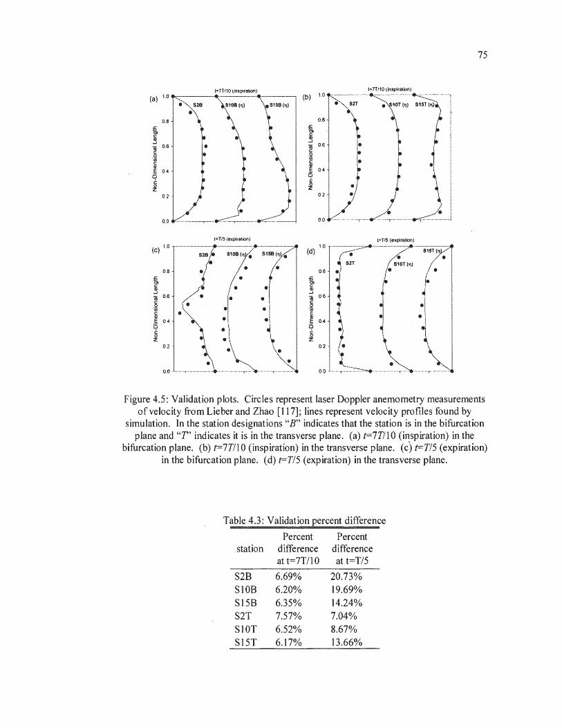
(a) 1.0
0,8
iii 0,6 c 0
' ii) c 4)
E 0.4
t=7T/10 (inspiration)
O J ) c i 02 ·
0
0 .0 ------.-~ - .,.,~ --
(c) 1.0 -
.r:: 0) c: Q) ...J
0,8
ni 0.6 c:
. Q (I) c
~ OA 0 § z
0.2
0.0 ·
• • •
t=T/5 (expiration)
S10B ('1 • 5158 (lll •
• • •
• • • •
• • • •
• •
t=7T/10 (inspiration)
(b: :: -.-~~~ l ~ ~ I r ~ ·1 I 8 0.4 ~ !
§ • I ,
z :: --=---~ _! t=T/5 (expiration)
(d) LO --;----~--------7 -S15T ~
J 0 6 ~ s~ tor,,, • • • j'' ~ .]· ~ 0 .4 6 c 0 z
0.2
0.0 • ,,, .... :=~-~ ...... . .... , .. , .. ,"'--. .............. T
75
Figure 4.5: Validation plots. Circles represent laser Doppler anemometry measurements of velocity from Lieber and Zhao [117] ; lines represent velocity profiles found by
simulation. In the station designations "B" indicates that the station is in the bifurcation plane and " T ' indicates it is in the transverse plane. (a) t=7T/10 (inspiration) in the
bifurcation plane. (b) t=7T/10 (inspiration) in the transverse plane. ( c) t=T/5 ( expiration) in the bifurcation plane. ( d) t=T/5 ( expiration) in the transverse plane.
Table 4.3: Validation percent difference
Percent Percent station difference difference
at t=7T/10 at t=T/5
S2B 6.69% 20.73% SlOB 6.20% 19.69% Sl5B 6.35% 14.24% S2T 7.57% 7.04% SlOT 6.52% 8.67% Sl5T 6.17% 13.66%
76
4.5. FLUID FLOW
Important flow features and turbulence will play a part in guiding the particles
along their paths through the domain. The presence and magnitude of the flow features
and turbulence vary throughout the respiratory cycle. This section will discuss important
fluid flow features observed in the results of the waveform simulations and look at the
role of turbulence in the domain throughout the respiratory cycle.
4.5.1. Important Fluid Structures. The dominant flow features that were
apparent throughout inspiration were:
(a) the jet caused by the endotracheal tube (ETI jet)
(b) the large rotating structure in the right main bronchus, and
( c) swirling flows in the bronchi.
The ETT jet is similar to the laryngeal jet which has been studied in the past [30,
82-85]. Both the laryngeal jet and the ETT jet cause a flow constriction and release fluid
into a larger environment at a high speed. The ETT jet is different from the jet caused by
the larynx because of its proximity to the carina and its range of orientation is dependent
upon how the tube was installed or how the patent is positioned. A structure similar to
the large rotating structure in the right main bronchus was reported by Xi et al [30] in the
trachea, and is believed to be caused by the laryngeal jet. The swirling flows in the
bronchi, at times, resemble Dean vorticies [122], however some of the swirling is thought
to result from the noncircular geometry of the airways as well as flow curvature effects.
The presence and the magnitude of the ETT jet, the large rotating structure in the right
main bronchi, and the swirling flows in the bronchi vary throughout the inspiratory
phase. During expiration the swirling in the bronchi remained and the endotracheal tube
caused a constriction in the flow as it exited the domain.
For purposes of demonstrating the presence and development of these flow
features the results from the flow control ascending ramp waveform were used. Velocity
vectors throughout the domain were plotted at several times. They are colored by
velocity magnitude and the size of the vectors scales with the velocity magnitude. Figure
4.6 shows the early stages of the ETT jet. It is clear that the jet is pointed towards the
right main bronchus due to the orientation of the endotracheal tube. An ETT jet pointed
towards the right main bronchus is common because path to the right main bronchus from
the trachea is more direct for most patients, although this depends largely upon how _the
ETT was installed. The large rotation in the right main bronchus has not yet developed
and swirling activity in slices L-L or R-R is not present at this early time (t=0.05 s).
Figure 4.7 demonstrates the development of the ETT jet. The jet has advanced to
just above slice R-R and is about to impinge on the wall of the right main bronchus. The
large rotation in the right main bronchus has still not developed and swirling activity in
slices L-L or R-R is not present at this time (t=0.075 s).
After the ETT jet impinges on the wall of the right main bronchus it begins to
disperse. Jet impingement and dispersion was observed by Choi [28]. Figure 4.8 shows
the dispersal of the ETT jet. A low grazing angle and the orientation of the surface where
the jet contacts the wall causes the jet to be deflected to the right lung; forming a
secondary jet. The maximum velocity in this secondary jet is much less than that of the
ETT jet. The shape of the ETT jet as it passes through slice R-R can be seen in Figure

4.8. The rotation in the right main bronchus begins to develop, but the swirling flow in
slice L-L is not yet present.
I~~--~~~~ ! -100 ~-~-~----.....;
0.0 1.0 2.0 3.0 4.0
time (s)
t=0.05 s
x Slice R-R
Velocity Magnitude (mis)
1.17 1.04 0.91 0.78 0.65 0.52 0.39 0.26 0.13 0.00
z
6-.
Slice L-L
78
Figure 4.6: Velocity vectors at time t=0.05 s. For the flow controlled ascending ramp waveform. Vectors ar~ colored by velocity magnitude.

i1EJc----; I -100 +---~-~-~---l
0.0 1.0 2.0 3.0 <4.0
time(•)
t=0.075 s
Velocity Magnitude (mis)
1.77 1.58 1.38 1.18 0.98 0.79 0.59 0.39 0.20 0.00
z
L.
_,,,_.-. ... ...--- --- y Slice L-L
79
Figure 4.7: Velocity vectors at time t=0.075 s. For the flow controlled ascending ramp waveform. Vectors are colored by velocity magnitude.
At t=0.2 s the secondary ( deflected) jet has impinged in the lower part of the right
main bronchus where the airway turns toward the anterior side of the patient which can
be seen in Figure 4.9. The jet disperses and there is no noticeable deflected jet. The
dispersed secondary jet begins to flow back upward to the airways of the right upper lobe
and to the left main bronchus. It is important to note that a large portion on the flow
entering the left main bronchus does not come directly from the ETT but rather, passes
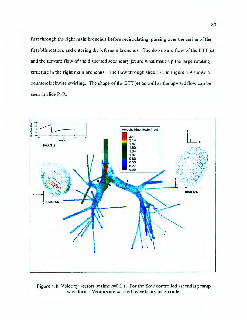
80
first through the right main bronchus before recirculating, passing over the carina of the
first bifurcation, and entering the left main bronchus. The downward flow of the ETT jet
and the upward flow of the dispersed secondary jet are what make up the large rotating
structure in the right main bronchus. The flow through slice L-L in Figure 4.9 shows a
counterclockwise swirling. The shape of the ETT jet as well as the upward flow can be
seen in slice R-R.
! 100
j ~Eb~-c .·~- ......------t··
·50 -· .. I -100 ---..--~--~- ....... 0.0 1.0 2.0 3.0 4.0
time(s)
t=0.1 s
•
Velocity Magnitude (mis)
2.41 2.14 1.87 1.60 1.34 1.07 0 .80 0.53 0.27 0.00
z
Lx
Figure 4.8: Velocity vectors at time t=0.1 s. For the flow controlled ascending ramp waveform. Vectors are colored by velocity magnitude.
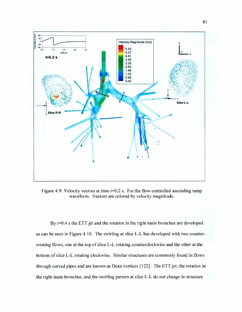
i1~ ---~~---i i -100 --~--------l
0.0 1.0 2.0 3.0 4.0
time (s)
t=0.2 s
Velocity Magnitude (m/s)
5.93 5.27 4.61 3.95 3.29 2.64 1.98 1.32 0.66 0.00
z
Lx
Figure 4.9: Velocity vectors at time t=0.2 s. For the flow controlled ascending ramp waveform. Vectors are colored by velocity magnitude.
81
By t=0.4 s the ETT jet and the rotation in the right main bronchus are developed
as can be seen in Figure 4.10. The swirling at slice L-L has developed with two counter-
rotating flows, one at the top of slice L-L rotating counterclockwise and the other at the
bottom of slice L-L rotating clockwise. Similar structures are commonly found in flows
through curved pipes and are known as Dean vortices [ 122]. The ETT jet, the rotation in
the right main bronchus, and the swirling pattern at slice L-L do not change in structure
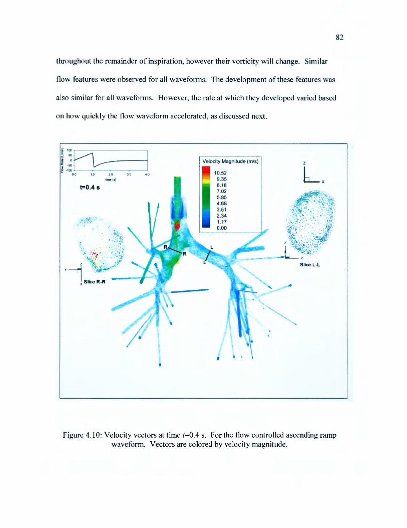
82
throughout the remainder of inspiration, however their vorticity will change. Similar
flow features were observed for all waveforms. The development of these features was
also similar for all waveforms. However, the rate at which they developed varied based
on how· quickly the flow waveform accelerated, as discussed next.
1 00 ~~~~~~~~~
50
0
.50
1.0 2.0 3.0
time (s)
t=0.4 s
4.0
Velocity Magnitude (m/s)
10.52 9.35 8.18 7.02 5.85 4.68 3.51 2.34 1.17 0.00
z
Lx
Slice L-L
Figure 4.10: Velocity vectors at time t=0.4 s. For the flow controlled ascending ramp waveform. Vectors are colored by velocity magnitude.
83
The velocity vectors throughout the domain for the pressure controlled sinusoidal
waveform near the end of inspiration (t=l.8 s) are shown in Figure 4.11. The flow rate is
similar to that of the flow controlled ascending ramp waveform at t=O. l s (Figure 4.8).
The ETT jet, the rotation in the right main bronchus, and the swirling pattern at slice L-L
are all developed in Figure 4.11 and resemble those at t=0.4 s for the flow controlled
ascending ramp waveform (Figure 4.10). It is clear that the presence and strength of the
flow features are not only dependent upon the inspiratory flow rate, but also the history of
the flow.
The fluid flow features throughout expiration are very similar for all of the
waveforms due to the nearly identical waveform shapes during expiration. The pressure
controlled sinusoidal waveform was different than the others for expiration; however, the
flow features were still similar. The velocity vectors throughout the domain for the
pressure controlled constant waveform at peak expiration are shown in Figure 4.12. The
swirling in slice L-L can still be seen in Figure 4.12 as well as the constriction in the flow
as it entered the endotracheal tube. When flow from a daughter branch enters the parent
branch it forms a small jet-like structure. This is most noticeable when there is a sharper
transition in airway diameter. In the present model these small jets are most visible in
Figure 4.12 in the most distal branches of the right and left upper lobes. These jets
dissipate very quickly due to the smooth transitional shapes of the bifurcations and are
more noticeable at higher flow rates.
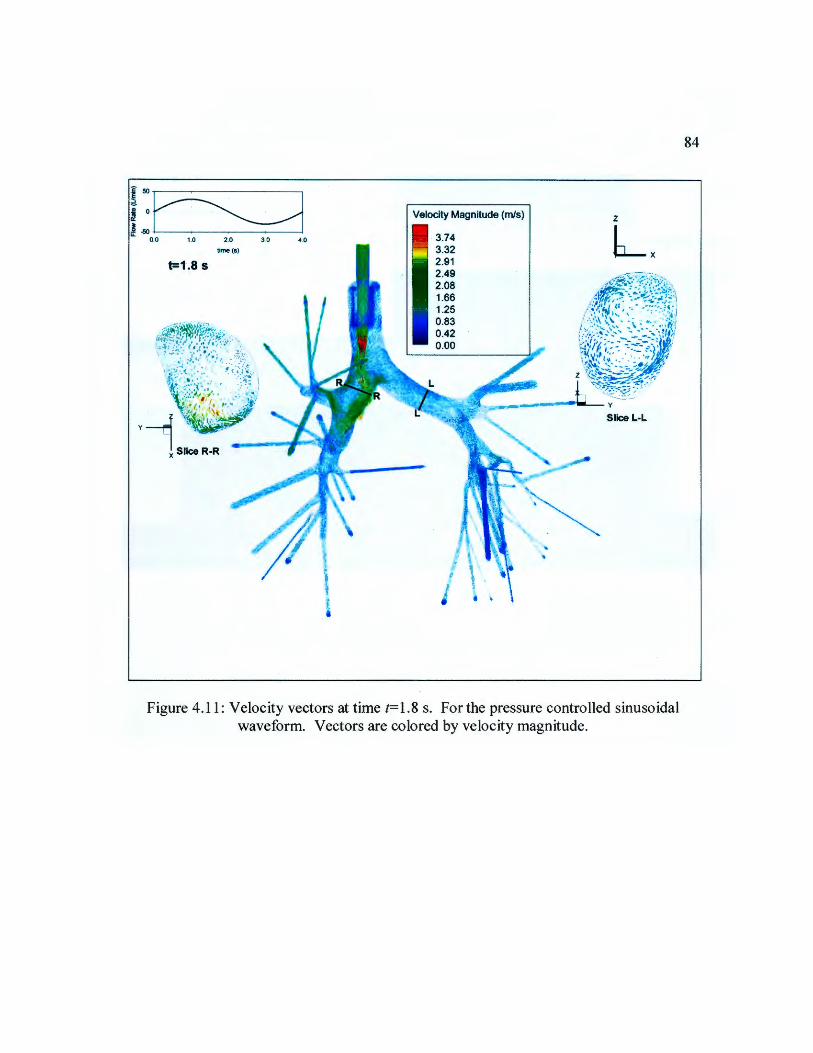
[ t=S-;d ...
Velocity Magnitude (mis)
3.74 3.32 2.91 2.49 2.08 1.66 1.25 0.83 0.42 0.00
z
L . 0.0 1.0 2.0 3.0 4.0
time(S)
Slice L·L
Figure 4.11: Velocity vectors at time t=l.8 s. For the pressure controlled sinusoidal waveform. Vectors are colored by velocity magnitude.
84

¥ 100
~ 50
i O ·50 ! -100 +---~-~--~---l
0.0 1~ ~o 10 4 .0
time(s)
t=1.1 s
Velocity Magnitude (m/s) z
L x
Slice L-L
Figure 4.12: Velocity vectors at time t=l.1 s. For the pressure controlled constant waveform. Vectors are colored by velocity magnitude.
4.5.2. Turbulence. To characterize flow turbulence, turbulence kinetic energy
(TKE) and vorticity were evaluated in slices through the domain. Turbulent kinetic
energy k is defined as:
85
(4.5)

where the prime symbol indicates a fluctuation and the overbar indicates a mean.
Vorticity, w, is defined as:
m=Vxu
86
(4.6)
Contours ofTKE for each waveform at peak inspiration are shown in Figure 4.13
and Figure 4.14 (e-g). There is a strong TKE around the edges of the ETT jet. TKE in
the human airways downstream of a jet (laryngeal) has been reported by Lin [83]. The
ETT jet is released far below the larynx in the trachea and, in this study, is aligned with
the opening of the right main bronchus. Because of the position and orientation of the
ETT, the TKE remains strong much lower into the airways when compared with the TKE
caused by the laryngeal jet. In addition, there is much more TKE in the right lung.
As the ETT jet impinges and deflects the TKE begins to dissipate rapidly similar
to the dissipation seen after the laryngeal jet impinges on the back of the trachea [83].
The areas of highest TKE are those where the incoming ETT jet begins to interact with
the deflected and dispersed flow coming upward out of the right main bronchus and
across the path of the ETT jet. A similar flow pattern was reported by Xi where the
highest turbulence viscosity ratio in the flow was reported [30]. High TKE remains
throughout most of the portion of the right lung modeled in this study and through some
of the left main bronchus. In general the TKE is stronger with the waveforms that have a
higher maximum flow rate. The patterns of TKE throughout the domain for the different
waveforms are similar.

t-0.1 •
(a)
t-1 .0 •
(c)
I t.
f
I t •
f
Turbulenc&K,nelk:E11«11y (Jikg)
t •
' '
L.
t
•
' '
(b)
f " ; ;n,---1., .. ,,,· ;, ;, " .,
t-0.4 s
(d)
I t .
f
I t .
f
87
z
6-.
SlceU.
t •
' '
L.
SllceU.
t •
' '
Figure 4.13: Contours of turbulence kinetic energy. For (a) pressure controlled constant at peak inspiration, (b) pressure controlled exponential at peak inspiration, ( c) pressure
controlled sinusoidal at peak inspiration, and (d) volume controlled ramp at peak inspiration
The TKE for the pressure controlled constant waveform at peak expiration is
shown in Figure 4.14 (h) as an example. The TKE contours for the other waveforms
were very similar to the pressure controlled constant case. The TKE for the pressure
controlled sinusoidal waveform was also similar in structure but had lower values of
TKE. The TKE present in inspiration is stronger than the turbulence for expiration (,...., 1.5
times) even though the peak flow rate for inspiration is on average about 97% of the peak

88
flow rate during expiration. The difference in the TKE during inspiration and expiration
is attributed to the presence of the ETT jet. Areas of highest TKE in expiration occur
when the flows from the daughter braches into the parent branches begin to mix and in
the ETT where.the flow is suddenly constricted creating a high flow velocity. The
production of TKE due to the mixing of daughter branch flows can be seen in Figure 4.14
(h) in the upper right lobe and in the left main bronchus for example.
t-0 .5 s
(e)
t-0 .1 s
(g)
• • • f
• ' . f
Turt)u leoce Kinetic Energy (J,1i.g}
• •
. '
Turt>ukmce Kinetic Energy {J/kg}
• • ' I
t-1 .0 s
SHot L--L
(f)
ts1 .1 s
SliceL-L
x Slice R -R
(h)
' • •
• '. r
L x
• • ' I
z
L .
• • ' I
Figure 4.14: Contours of turbulence kinetic energy. For (e) volume controlled sigmoid at peak inspiration, (f) flow controlled ascending ramp peak inspiration, (g) flow controlled descending ramp peak inspiration, and (h) pressure controlled constant at peak expiration
89
Contours of vorticity for each waveform at peak inspiration are shown in Figure
4.15 and Figure 4.16 ( e-g). Higher vorticity exists in the right lung in inspiration for
every waveform due to the ETT jet. Areas of high vorticity exist in the middle of the
domain around the edges of the ETT jet and at the walls of the domain. Higher near wall
vorticity exists where higher near wall velocities are present. One area of high vorticity
exists where the ETT jet impinges and deflects off the wall of the right main bronchus
(See Figure 4.15 and Figure 4.16 e-g). In the waveforms with higher peak flow rates (i.e.
pressure controlled constant, flow controlled ascending ramp, and flow controlled
descending ramp) the vorticity suddenly drops near the bottom of the wall where the ETT
jet is being deflected as the secondary jet detaches from the wall (Figure 4.15 (a) Figure
4.16 (f) and (g)). This behavior is not observed in the waveforms with a lower flow rate.
A similar pattern occurs at the first bifurcation as the flow coming from the right lung
passes over the carina. Another patch of high vorticity is observed at the top of the left
main bronchus.
Contours of vorticity for the pressure controlled constant waveform at peak
expiration are shown in Figure 4.16 (h) as an example. For the other waveforms,
vorticity was very similar in expiration. Expiration for the pressure controlled sinusoidal
waveform had vorticity that was also similar in structure but had smaller values for
vorticity. The highest vorticity for expiration existed in the ETT where the highest
velocity existed. Vorticity was also present in the left main bronchus where there was
more significant swirling motion due to geometry.

90
! ':~ Vorticity Magnitude (radii) L: ..... -.- -.. - .. Vorticity Magnitude (radls) z
9.9551E+03 6. t464E+03 6-. 8.8490E•03 5 4634E+03
t-0 .1 s 7 H29E+03 tz0.4 s 4 7605E+03 66367E•03 • 0976E•03
~ 5 5306E•03 3 4146E+03 4 4245E+03 2 7317E•03 3.3t84E+03 2.0488E+03 2 2t22E +03 1 3659E+03 1.t061E+03 6.8293E+02 O.OOOOE+OO O.OOOOE+OO
sac.L-l. Sbl·L
• • • • I • • • • ' I • ' • •
(a) (b)
! ,. I :~ ·~ Vorticity Magnitude (•odls) Voruo ty MogMude (,8<1/s) 2
I -«)'lO --- ; ;,-- :.~ ;-; ~g 3 3686E•03 i .:.t ;; ,·, .~ .t • 4643E+03 L . - ,~ 2.9944E•03 3.9860E+03
t-1 .0s 2.6201E•03 t-0.4 s 3.4878E•03 2.2458E+03 2 9895E+03 1.8715E+03 2.4913E+03 1.4972E+03 1 9930E+03 1.1229E+03 1 4948E+03
~ 7 4859E•02 9 9651E+02 3 7429E+02 4 9826E•02 O OOOOE• OO O OOOOE+OO
L~ 8- L·L S-L-l.
• • • . • I • • • ' '
(c) (d)
Figure 4.15: Contours of vorticity. For (a) pressure controlled constant at peak inspiration, (b) pressure controlled exponential at peak inspiration, ( c) pressure controlled
sinusoidal at peak inspiration, and (d) volume controlled ramp at peak inspiration
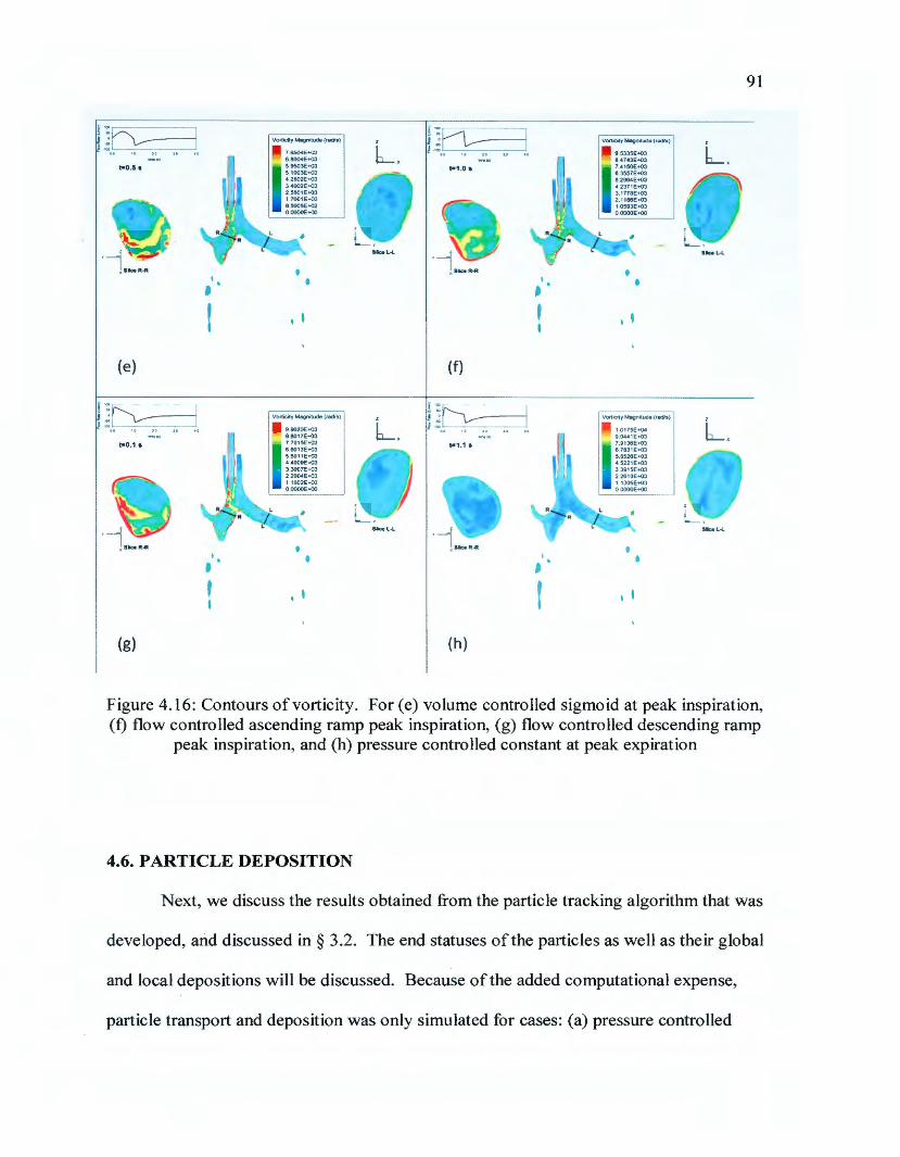
91
! ':~ I 7 , ~ 5 "'
.1.;::~1, - , , - a ,o •o
Vorticity Magnitude (rad/s) z I • Vor1icity Magnitude (radls) z 7.6504E+03 6-. J .,:.. " " " .. 9.5335E+03 6-.. 6.8004E+03 8.4743E+03
t-0.5 s 5.9503E•03 1=1 .0 s 7 4150E•03 5 1003E•03 6.3557E• 03 • 2502E•03 6.2964E+03 3.4002E+03 • 237 1E•03 2.5501E+03 3.1778E+03 1.7001E+03 2.1186E +03 8 ,5005E+02 1.0593E+03 O.OOOOE+OO O.OOOOE+OO
Slce L-1. Sb L-1 .
• • ' • • . • •• • f • • ' • ' •
(e) (f)
I ':~ !}~ , ' : ,:, ·---:;~ -· ;; ;, }, Vor1 icity Magnitude (rad/s) z v0r1;c.1y Mogn~ude (radio) z
9 .9020E•03 6-. 1 0175E•04 6-.. 8.80 17E•03 9.0441E•03
t-0 .1 s 7.7015E•03 t-1 .1 s 7.9136E•03 6 .6013E+03 6.7831E+03 5.501 1E+03 5.6526E+03 4 .4009E+OO '4 5221E+03 3.3007E+03 3.3915E+03 2 2004E+03 2.2610E•03 1 1002E•03 1 1305E•03 OOOOOE+OO OOOOOE•OO
Slic:eL·L S-L·L
• ' ' . • I • • • • ' • • f • I I
(g) (h)
Figure 4.16: Contours of vorticity. For (e) volume controlled sigmoid at peak inspiration, (f) flow controlled ascending ramp peak inspiration, (g) flow controlled descending ramp
peak inspiration, and (h) pressure controlled constant at peak expiration
4.6. PARTICLE DEPOSITION
Next, we discuss the results obtained from the particle tracking algorithm that was
developed, and discussed in§ 3.2. The end statuses of the particles as well as their global
and local depositions will be discussed. Because of the added computational expense,
particle transport and deposition was only simulated for cases: (a) pressure controlled
92
constant, (b) pressure controlled sinusoidal, (c) volume controlled ramp, and (d) flow
controlled ascending ramp waveforms. The pressure controlled constant and volume
controlled ramp cases were selected because they are the most frequently used, the
pressure controlled sinusoidal waveform was chosen because of the low flow rates, and
the flow controlled ascending ramp case was selected because it had similar peak flow
rates to the pressure controlled constant case, but the shape of the flow rate curve is very
nearly reversed in time during inspiration.
4.6.1. Particle End Status. Particles that were injected into the domain took on
one of five end statuses: (1) deposited on the walls, (2) escaped through one of the
outlets, (3) exceeded the particle tracking distance limit (100 m), (4) exceeded the
maximum number of integration steps (1 x 10⁶ steps), or ( 5) encountered an integration
error. The integration errors occur when the particle velocity is too small ( ~o) and may
occur when a particle is injected very close to the wall with a velocity ~o. Particles may
have exceeded the distance limit or the maximum number of integration steps when
caught in a recirculation zone.
The overall particle end statuses for each simulation are summarized in Table 4.4.
In all four cases, the number of particles that neither deposited nor escaped was <5%.
Particles that are deposited on the walls of the model are assumed to flow with the mucus
lining and rendered ineffective as medication [123]. Particles escaping from the domain
to the lower airways have a chance of depositing in the lower airways or diffusing into
the bloodstream for systemic delivery. There have been studies conducted to investigate
particle .deposition in the lower airways; however these studies do not focus on the effect
of inspiratory waveform [64, 124-125]. Of the waveforms in this study, the waveform
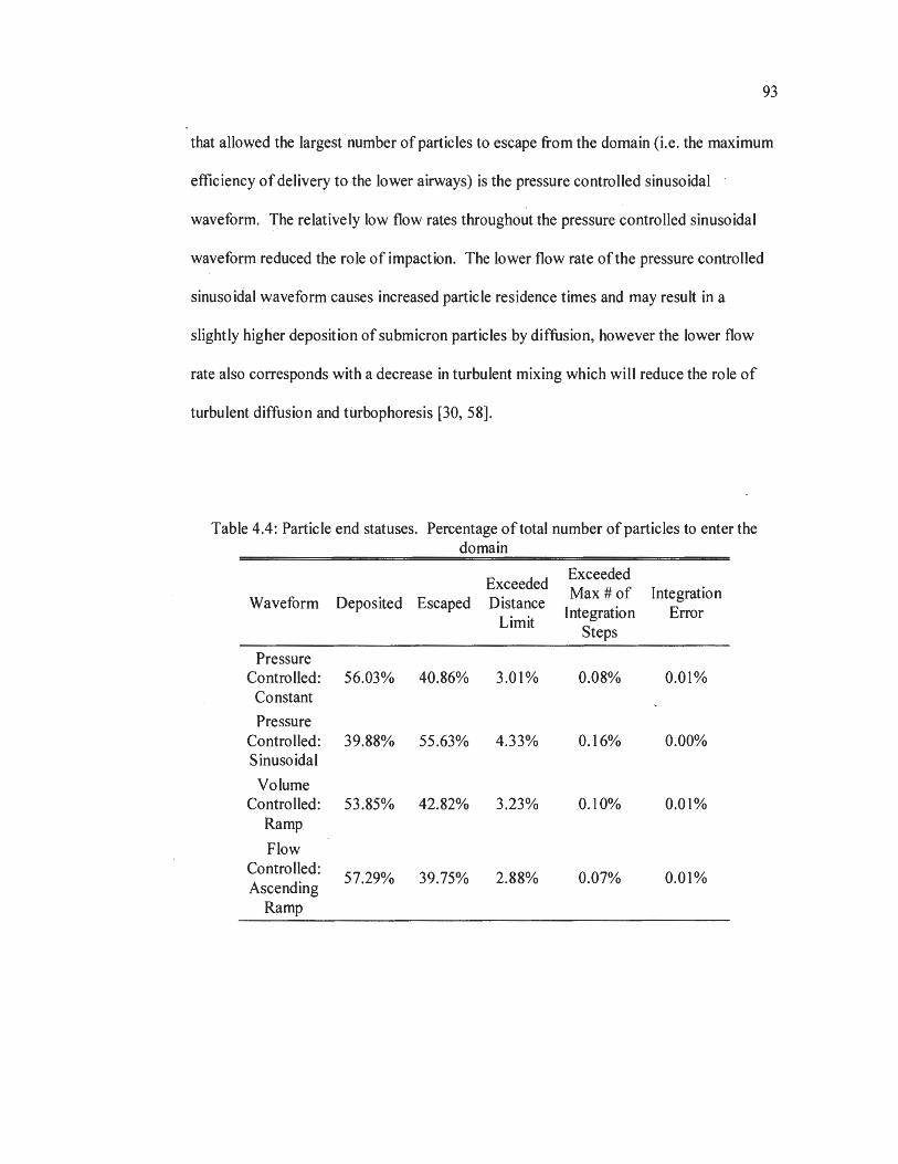
93
that allowed the largest number of particles to escape from the domain (i.e. the maximum
efficiency of delivery to the lower airways) is the pressure controlled sinusoidal ·
waveform. The relatively low flow rates throughout the pressure controlled sinusoidal
waveform reduced the role of impaction. The lower flow rate of the pressure controlled
sinusoidal waveform causes increased particle residence times and may result in a
slightly higher deposition of submicron particles by diffusion, however the lower flow
rate also corresponds with a decrease in turbulent mixing which will reduce the role of
turbulent diffusion and turbophoresis [30, 58].
Table 4.4: Particle end statuses. Percentage of total number of particles to enter the domain
Exceeded Exceeded
Waveform Deposited Escaped Distance Max#of Integration
Integration Error Limit
Steps
Pressure Controlled: 56.03% 40.86% 3.01% 0.08% 0.01%
Constant
Pressure Controlled: 39.88% 55.63% 4.33% 0.16% 0.00% Sinusoidal
Volume Controlled: 53.85% 42.82% 3.23% 0.10% 0.01%
Ramp
Flow Controlled:
57.29% 39.75% 2.88% 0.07% 0.01% Ascending
Ramp
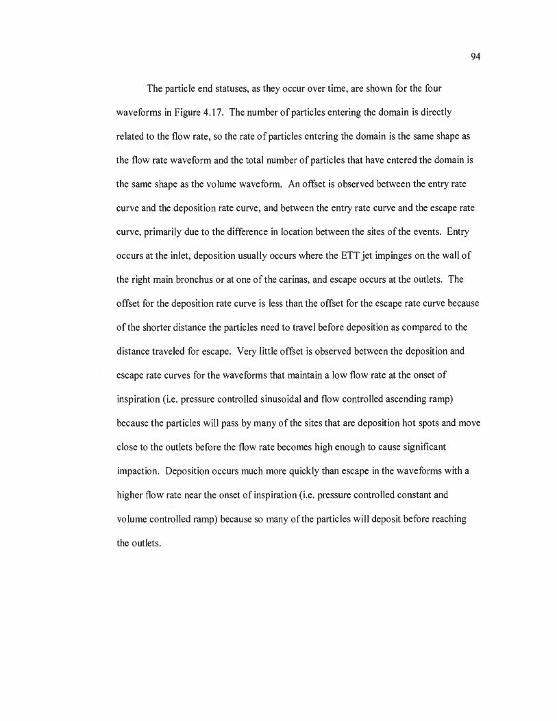
94
The particle end statuses, as they occur over time, are shown for the four
waveforms in Figure 4.17. The number of particles entering the domain is directly
related to the flow rate, so the rate of particles entering the domain is the same shape as
the flow rate waveform and the total number of particles that have entered the domain is
the same shape as the volume waveform. An offset is observed between the entry rate
curve and the deposition rate curve, and between the entry rate curve and the escape rate
curve, primarily due to the difference in location between the sites of the events. Entry
occurs at the inlet, deposition usually occurs where the ETT jet impinges on the wall of
the right main bronchus or at one of the carinas, and escape occurs at the outlets. The
offset for the deposition rate curve is less than the offset for the escape rate curve because
of the shorter distance the particles need to travel before deposition as compared to the
distance traveled for escape. Very little offset is observed between the deposition and
escape rate curves for the waveforms that maintain a low flow rate at the onset of
inspiration (i.e. pressure controlled sinusoidal and flow controlled ascending ramp)
because the particles will pass by many of the sites that are deposition hot spots and move
close to the outlets before the flow rate becomes high enough to cause significant
impaction. Deposition occurs much more quickly than escape in the waveforms with a
higher flow rate near the onset of inspiration (i.e. pressure controlled constant and
volume controlled ramp) because so many of the particles will deposit before reaching
the outlets.
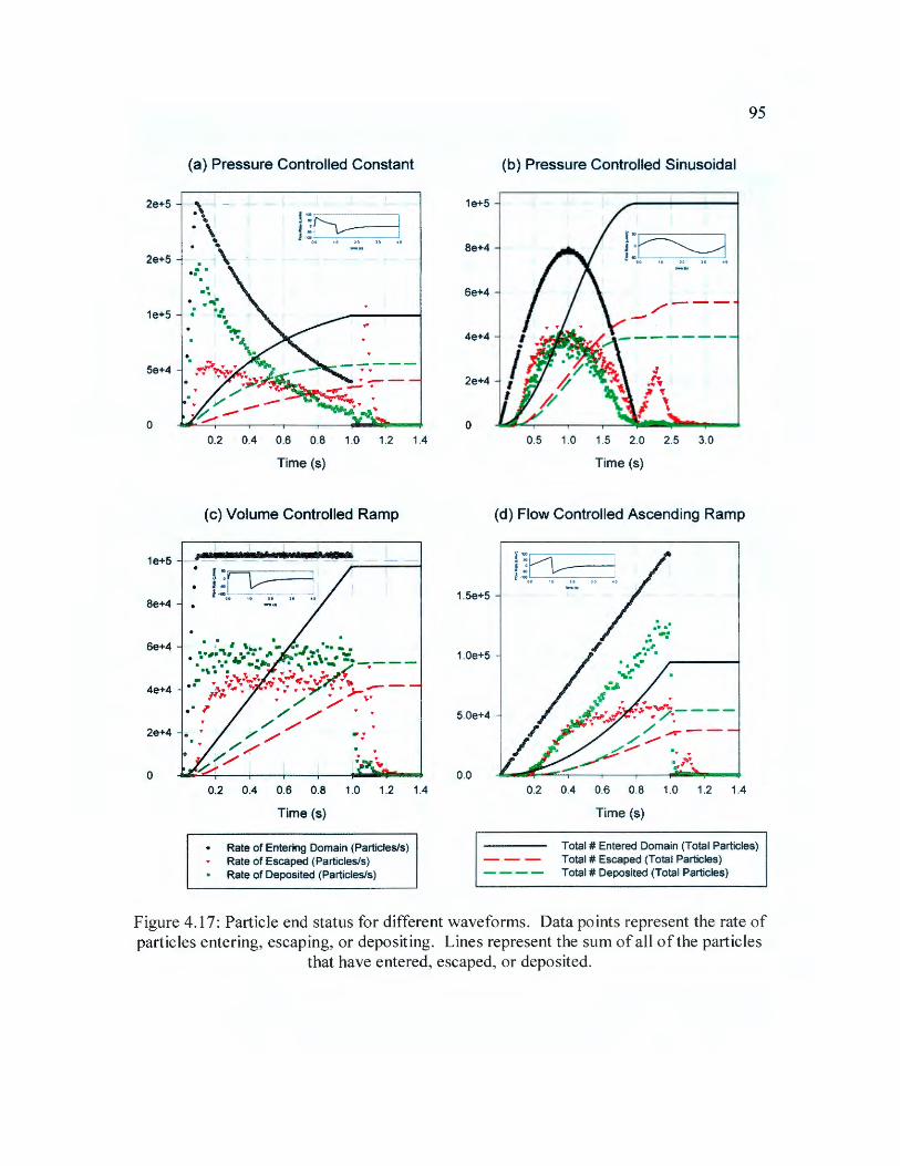
2e+5
2e+5
1e+5
5e+4
0
1e+5
8e+4
6e+4
4e+4
2e+4
0
(a) Pressure Controlled Constant
0.2 0.4 0.6 0.8 1.0 1.2 1.4
Time (s)
( c) Volume Controlled Ramp
. .• . . t., , ......... · .... . . i:.·-· .. \,.. .. •"' ·""·\· . '=' ............... ""' ... -,,;:---.,~ . .. ... ~ . ~ . • ~ .. :/~./'-· .... d'":'~··,:._f>I_... -- ~. __ ., . ~ .. . . . . .,,,, . . r .,,,....
,~~ .. / / " .. .. ,, / / .... / /
.. / ~ / ('/ ~. .. ..
• -:. l
0.2 0.4 0.6 0.8 1.0 1.2 1.4
Time (s)
Rate of Entering Domain (Particles/s) Rate of Escaped (Particles/s) Rate of Deposited (Particles/s)
1e+5
8e+4
6e+4
4e+4
2e+4
0
1.5e+5
1.0e+S
5.0e+4
0.0
(b) Pressure Controlled Sinusoidal
,---
Q5 1.0 1.5 2.0 2.5 3.0
Time (s)
(d) Flow Controlled Ascending Ramp
0.2 0.4 0.6 0.8 1.0 1.2 1.4
Time (s)
95
Total# Entered Domain (Total Particles) Total# Escaped (Total Particles) Total# Deposited (Total Particles)
Figure 4.17: Particle end status for different waveforms. Data points represent the rate of particles entering, escaping, or depositing. Lines represent the sum of all of the particles
that have entered, escaped, or deposited.

96
The slope of the· deposition rate curve generally fo Hows the flow rate curve. An
increase in flow rate causes increased deposition because of the increased number·of
particles entering the domain and because of the increase in impaction, turbulent
dispersion and turbophoresis. The escape rate also increases with the flow rate but the
slope of the escape rate curve does not keep up with the slope of the flow rate curve at
higher flow rates because of the higher number of particles depositing before reaching the
outlets. This is most easily observed in Figure 4.17 ( d) where there is clear separation of
the deposition and the escape rate curves at approximately t=0.5 s.
At peak expiration, the deposition rates in Figure 4.17 are much lower than at
peak inspiration, despite the high flow rates. This behavior is due to the decrease in
potential impaction sites (most notably the carinas) and the reduction in turbulence
(Figure 4.14) including the absence of the large recirculation zone in the right main
bronchus (Figure 4.12). The reduction in the deposition rate along with the high flow
rate causes a high escape rate in expiration (Figure 4.17). An additional factor that
contributes to the high escape rate at peak expiration is the higher percentage of small
particles that did not impact in inspiration. In the pressure controlled constant (Figure
4.17 (a)) and volume controlled ramp (Figure 4. l 7(c)) waveforms the highest escape rate
is reached in expiration because of the large population of particles in the domain just
before expiration. This high population of particles can be seen in Figure 4.18 and is
caused by a long period of low flow rate. The pressure controlled sinusoidal waveform
also has a large population of particles just before expiration and high escape rate is still
seen despite the slow flow acceleration.
c ·ro E 0
8000
0 6000 c (/) a, 0 t: ~ 4000
0 '-Q.) .c E ~ 2000
0.5 1.0
.... . r ··~~·ll" " ·~ ,1, • t •
• • ,· ! ~
l ~ ' :
~ i • f : ... l . : l . . . . .
1.5 2.0 2.5
Time (s)
Pressure Control: Constant • • • • • • • • • • • • • • • Pressure Control: Sinusoidal - - - - - - • Volume Control: Ramp - • • - • • - • • Flow Control: Ascending Ramp
3.0
1 I ~. ·-·r---~ I I
Figure 4.18: Number of particles in the domain as a function of time
4.6.2. Global Deposition. The most commonly used parameter to characterize
global particle deposi_tion is the deposition fraction, defined as the ratio of number of
particles that have deposited in the ·domain to the number of particles that have entered
the domain. The overall deposition fraction for each simulation is given in Table 4.5.
The deposition fractions for the pressure controlled constant and the flow controlled
ascending ramp waveforms were found to be similar at -56 %. Because the volume
97
controlled ramp waveform does not reach as high of a flow rate, the deposition fraction is
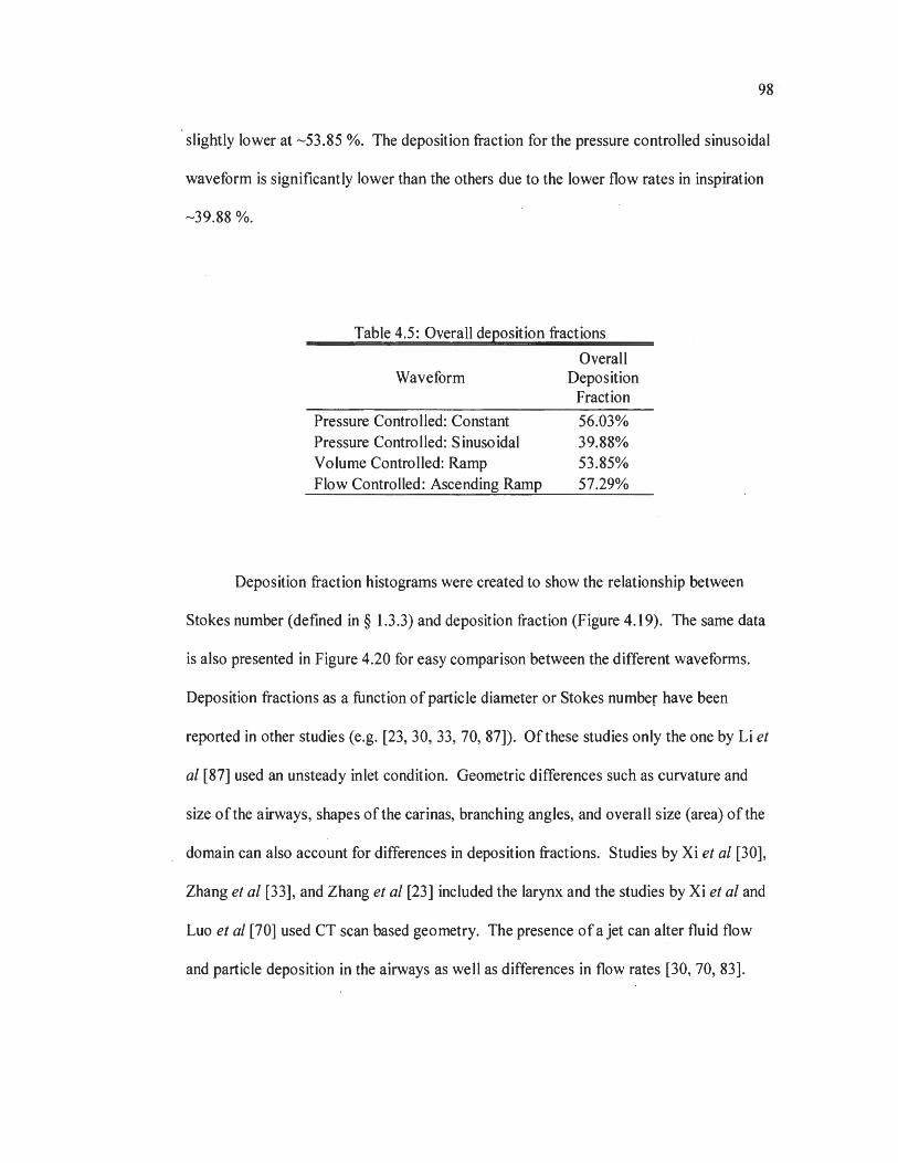
98
slightly lower at --53.85 %. The deposition fraction for the pressure controlled sinusoidal
waveform is significantly lower than the others due to the lower flow rates in inspiration
--39.88 %.
Table 4.5: Overall deposition fractions
Overall Waveform Deposition
Fraction
Pressure Controlled: Constant 56.03% Pressure Controlled: Sinusoidal 39.88% Volume Controlled: Ramp 53.85% Flow Controlled: Ascending Ramp 57.29%
Deposition fraction histograms were created to show the relationship between
Stokes number ( defined in § 1.3.3) and deposition fraction (Figure 4.19). The same data
is also presented in Figure 4.20 for easy comparison between the different waveforms.
Deposition fractions as a function of particle diameter or Stokes number have been
reported in other studies (e.g. [23, 30, 33, 70, 87]). Of these studies only the one by Li et
al [87] used an unsteady inlet condition. Geometric differences such as curvature and
size of the airways, shapes of the carinas, branching angles, and overall size (area) of the
domain can also account for differences in deposition fractions. Studies by Xi et al [30],
Zhang et al [33], and Zhang et al [23] included the larynx and the studies by Xi et al and
Luo et al [70] used CT scan based geometry. The presence of a jet can alter fluid flow
and particle deposition in the airways as well as differences in flow rates [30, 70, 83].
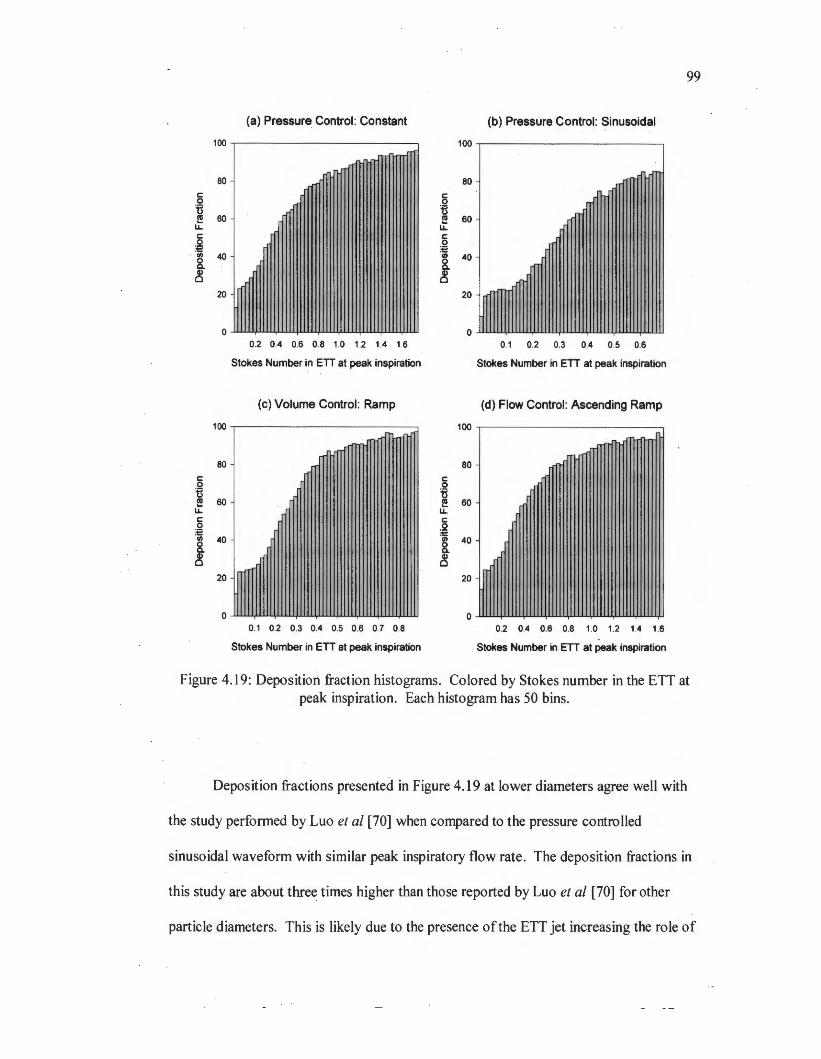
c 0 u
80
e 60 IL. c 0
· j 40 &. ~
c 0 u
20
80
e 60 IL. c ~ ·u; 40 8. ~
20
(a) Pressure Control: Constant
0.2 0.4 0.6 0.8 1.0 1.2 1.4 1.6
Stokes Number in ETI at peak inspiration
(c) Volume Control: Ramp
0.1 0.2 0.3 0.4 0.5 0.6 0. 7 0.8
Stokes Number in ETI at peak inspiration
(b) Pressure Control: Sinusoidal
100 ~------------,
c 0 u
80
e 60 IL. c 0 E "' 40 8. ~
c .Q t,
80
e 60 IL. c .Q :t::: "' 40 &. ~
20
0
0.1 0.2 0.3 0.4 0.5 0.6
Stokes Number in ETI at peak inspiration
(d) Flow Control: Ascending Ramp
0.2 0.4 0.6 0.8 1.0 1.2 1.4 1.6
Stokes Number in ETI at peak inspiration
99
Figure 4.19: Deposition fraction histograms. Colored by Stokes number in the ETT at peak inspiration. Each histogram has 50 bins.
Deposition fractions presented in Figure 4.19 at lower diameters agree well with
the study performed by Luo et al [70] when compared to the pressure controlled
sinusoidal waveform with similar peak inspiratory flow rate. The deposition fractions in
this study are about thre~ times higher than those reported by Luo et al [70] for other
particle diameters. This is likely due to the presence of the ETT jet increasing the role of
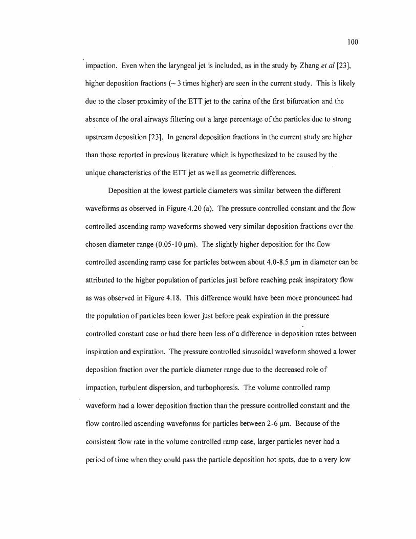
100
impaction. Even when the laryngeal jet is included, as in the study by Zhang et al [23],
higher deposition fractions (- 3 times higher) are seen in the current study. This is likely
due to the closer proximity of the ETT jet to the carina of the first bifurcation and the
absence of the oral airways filtering out a large percentage of the particles due to strong
upstream deposition [23]. In general deposition fractions in the current study are higher
than those reported in previous literature which is hypothesized to be caused by the
unique characteristics of the ETT jet as well as geometric differences.
Deposition at the · lowest particle diameters was similar between the different
waveforms as observed in Figure 4.20 (a). The pressure controlled constant and the flow
controlled ascending ramp waveforms showed very similar deposition fractions over the
chosen diameter range (0.05-10 µm). The slightly higher deposition for the flow
controlled ascending ramp case for particles between about 4.0-8.5 µm in diameter can be
attributed to the higher population of particles just before reaching peak inspiratory flow
as was observed in Figure 4.18. This difference would have been more pronounced had
the population of particles been lower just before peak expiration in the pressure
controlled constant case or had there been less of a difference in deposition rates between
inspiration and expiration. The pressure controlled sinusoidal waveform showed a lower
deposition fraction over the particle diameter range due to the decreased role of
impaction, turbulent dispersion, and turbophoresis. The volume controlled ramp
waveform had a lower deposition fraction than the pressure controlled constant and the
flow controlled ascending waveforms for particles between 2-6 µm. Because of the
consistent flow rate in the volume controlled ramp case, larger particles never had a
period of time when they could pass the particle deposition hot spots, due to a very low

101
flow rate. This is different than the pressure controlled constant and flow controlled
ascending ramp cases where higher flow rates existed, but there were also long periods of
very low flow rate that lowered the deposition fraction for particles larger than about 3
µm in diameter.
(a) 80
-~ c: 0
60 ~ e LL c: 0 :E 40
"' 0 Q.
~ 20
0
100
(b) 80
-~ ~ c: 0 60 ts e u. c: 0 :E 40 ~ Q.
~ 20
0
2
0.2
4 6
Particle Diameter (µm)
-t--- -
Pressure Control: Constant Pressure Control: Sinusoidal Volume Control: Ramp Flow Control: Ascending Ramp
8
.::-,---
Pressure Control: Constant - - - Pressure Control: Sinusoidal - - - - Volume Control: Ramp
Flow Control:Ascending Ramp
0.4 0.6 0.8 1.0 1.2 1.4 1.6
Stokes Number at Peak Inspiration
10
Figure 4.20: Deposition fraction (a) by particle diameter and (b) by Stokes number in the ETT at peak inspiration

102
4.6.3. Local Deposition. Local deposition is characterized qualitatively by
identifying particle deposition locations, and quantitatively by contours of depositipn
enhancement factor (DEF). Particle locations for the pressure controlled sinusoidal
waveform are shown in Figure 4.21. Similar particle deposition plots have been reported
in the literature [26, 30-31, 70, 87, 126]. All of these studies used a steady state inlet
condition, and only the study performed by Lambert et al [31] accounted for the
unsteadiness of turbulence. Particle deposition in realistic and simplified models of the
oral airways was studied· by Xi et al [26]. Lambert et al [31 ], Luo et al [70], and Xi et al
[30] studied particle deposition in CT scan based models of the upper tracheobronc~ial
region. Particle deposition in geometrically simplified airways was studied by Luo et al
[70] and Li et al [87]. Lambert et al [31 ], Xi et al [26], and Xi et al [30] included the
larynx.
Several deposition hot spots are visible in Figure 4.21: the site where the ETT jet
impinges and deflects off of the wall of the right main bronchus, the site where the
deflected jet impinges on the wall of the right main bronchus, the walls surrounding the
large rotating structure in the right main bronchus, the superior wall of the branch leading
to the right upper lobe, the superior wall of the left main bronchus near the first
bifurcation, and the carinas of the bifurcations.
103
!'~~ -------; a:::: -50 i -100 +------,------.----~----1 0 .0 1.0 2 .0 3.0 4 .0
time(s)
...
Figure 4.21: Deposition locations for the pressure controlled sinusoidal waveform. Key deposition hot spots are labeled as: (1) Site of impingement and the site where the ETT
jet impinges and deflects off of the wall of the right main bronchus, (2) the site where the deflected jet impinges on the wall of the right main bronchus, (3) the walls surrounding
the large rotating structure in the right main bronchus, ( 4) the superior wall of the branch leading to the right upper lobe, (5) the superior wall of the left main bronchi near the first
bifurcation, (6) the carinas of the right lung e.g. (7) and the carinas of the left lung e.g.
The deposition at the impingement sites of the ETT jet is caused by impaction
similar to the impaction reported by Xi et al [26] with a difference being that the
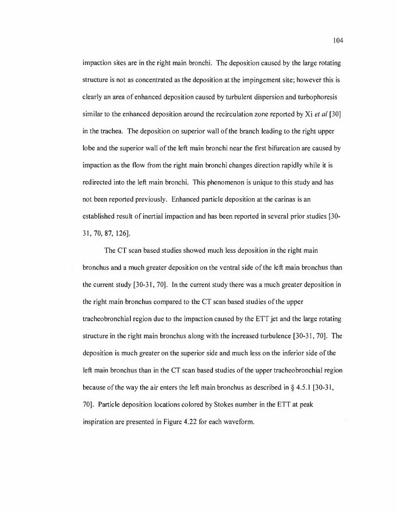
104
impaction sites are in the right main bronchi. The deposition caused by the large rotating
structure is not as concentrated as the deposition at the impingement site; however this is
clearly an area of enhanced deposition caused by turbulent dispersion and turbophoresis
similar to the enhanced deposition around the recirculation zone reported by Xi et al [30]
in the trachea. The deposition on superior wall of the branch leading to the right upper
lobe and the superior wall of the left main bronchi near the first bifurcation are caused by
impaction as the flow from the right main bronchi changes direction rapidly while it is ·
redirected into the left main bronchi. This phenomenon is unique to this study and has
not been reported previously. Enhanced particle deposition at the carinas is an
established result of inertial impaction and has been reported in several prior studies [30-
31, 70,87, 126].
The CT scan based studies showed much less deposition in the right main
bronchus and a much greater deposition on the ventral side of the left main bronchus than
the current study [30-31, 70]. In the current study there was a much greater deposition in
the right main bronchus compared to the CT scan based studies of the upper
tracheobronchial region due to the impaction caused by the ETT jet and the large rotating
structure in the right main bronchus along with the increased turbulence [30-31, 70]. The
deposition is much greater on the superior side and much less on the inferior side of the
left main bronchus than in the CT scan based studies of the upper tracheobronchial region
because of the way the air enters the left main bronchus as described in § 4.5.1 [30-31,
70]. Particle deposition locations colored by Stokes number in the ETT at peak
inspiration are presented in Figure 4.22 for each waveform.
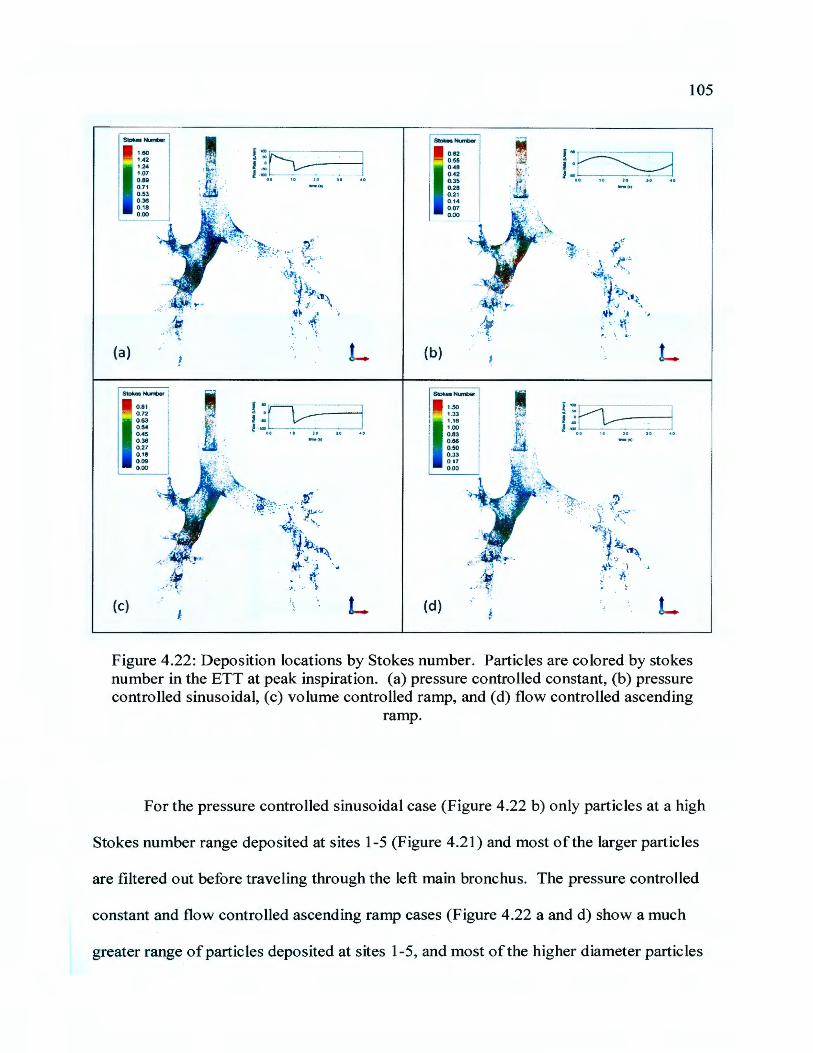
(a)
(c)
HIO 1.42 1.24 1.07 0 .89 0.71 0 .53 0 .38 0 .18 0 .00
0 .81 0.72 0 .63 0.54 0 .45 0 .38 0 .27 0.18 0 .09 0 .00
L.
f ~ M--=-----; l -100.~ J.
L
(b)
0.82 0.55 0 .48 0 .42 0 .35 0 .28 0 .21 0 .14 0.07 0.00
Stokes Number
(d)
1.50 1.33 1.16 1.00 0 .83 0.86 0 .50 0 .33 0 .17 0 .00
i
l ! 60
I • , .... ~. ---,.-~--' _,. (• I
j~~ ---f .,coo~
L
105
Figure 4.22: Deposition locations by Stokes number. Particles are colored by stokes number in the ETT at peak inspiration. (a) pressure controlled constant, (b) pressure controlled sinusoidal, (c) volume controlled ramp, and (d) flow controlled ascending
ramp.
For the pressure controlled sinusoidal case (Figure 4.22 b) only particles at a high
Stokes number range deposited at sites 1-5 (Figure 4.21) and most of the larger particles
are filtered out before traveling through the left main bronchus. The pressure controlled
constant and flow controlled ascending ramp cases (Figure 4.22 a and d) show a much
greater range of particles deposited at sites 1-5, and most of the higher diameter particles
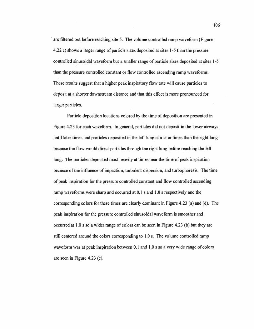
106
are filtered out before reaching site 5. The volume controlled ramp waveform (Figure
4.22 c) shows a larger range of particle sizes deposited at sites 1-5 than the pressure
controlled sinusoidal waveform but a smaller range of particle sizes deposited at sites 1-5
than the pressure controlled constant or flow controlled ascending ramp waveforms.
These results suggest that a higher peak inspiratory flow rate will cause particles to
deposit at a shorter downstream distance and that this effect is more pronounced for
larger particles.
Particle deposition locations colored by the time of deposition are presented in
Figure 4.23 for each waveform. In general, particles did not deposit in the lower a~ays
until later times and particles deposited in the left lung at a later times than the right lung
because the flow would direct particles through the right lung before reaching the left
lung. The particles deposited most heavily at times near the time of peak inspiration
because of the influence of impaction, turbulent dispersion, and turbophoresis. The time
of peak inspiration for the pressure controlled constant and flow controlled ascending
ramp waveforms were sharp and occurred at 0.1 sand 1.0 s respectively and the
corresponding colors for these times are clearly dominant in Figure 4.23 (a) and (d). The
peak inspiration for the pressure controlled sinusoidal waveform is smoother and
occurred at 1.0 s so a wider range ofcolors can be seen in Figure 4.23 (b) but they are
still centered around the colors corresponding to 1.0 s. The volume controlled ramp
waveform was at peak inspiration between 0.1 and 1.0 s so a very wide range of colors
are seen in Figure 4.23 ( c ).
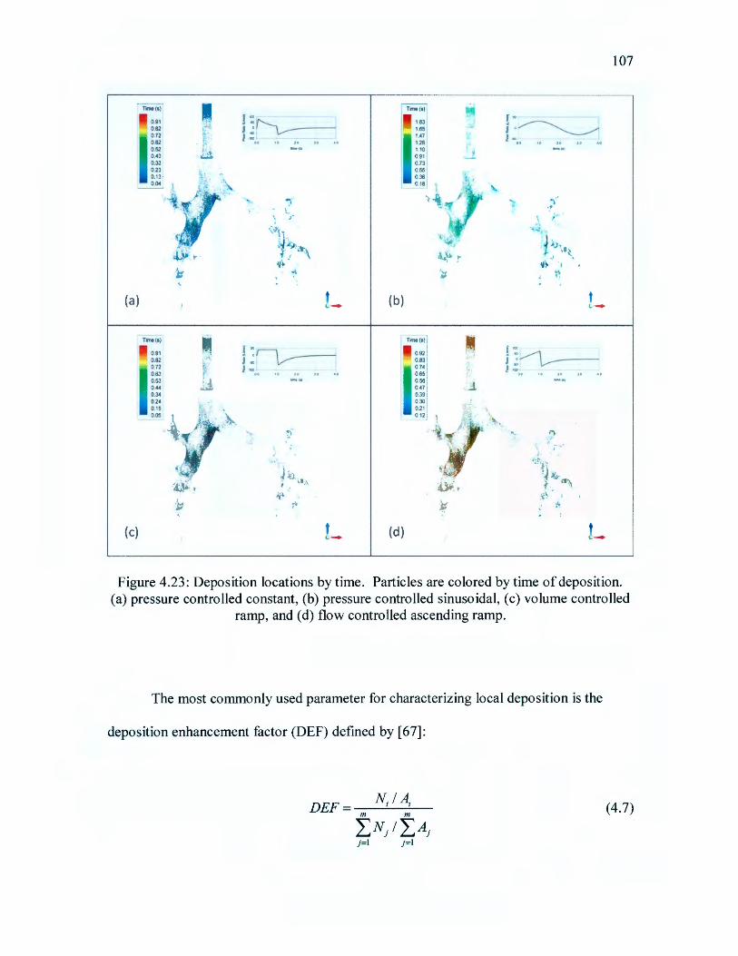
(a)
(c)
rme (s)
0.91 0.82 0.72 0 .62 0.52 0.43 0.33 0 .23 0.13 · 0.04
Time(s)
0.91 0.82 0.72 0.63 0.53 0.44 0.34 0.24 0.15 0.05
... ,• .
~,· - /
J '
!-~ ~ I ·00
010 1., }a
.,.,... lt}
(b)
(d)
rme (s)1
092 0.83
0741 0.65 0.56 047 0.39
~-~~ I 0 12
107
, .. ~ I ' , .~ 0 0 10 'JO )0 AO
'"
)~;-1 l \ I ,J ', ~.
... -
1
:\
Figure 4.23: Deposition locations by time. Particles are colored by time of deposition. (a) pressure controlled constant, (b) pressure controlled sinusoidal, (c) volume controlled
ramp, and (d) flow controlled ascending ramp.
The most commonly used parameter for characterizing local deposition is the
deposition enhancement factor (DEF) defined by [ 67]:
(4.7)
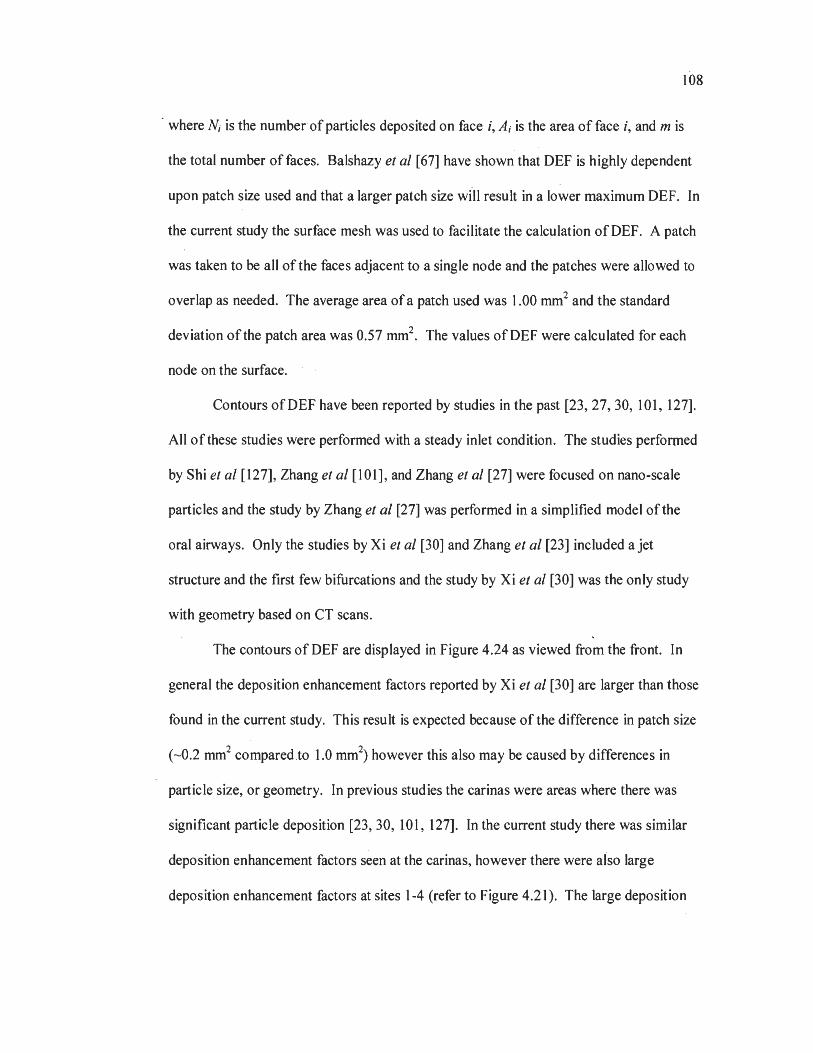
108
where N; is the number· of particles deposited on face i, A; is the area of face i, and m is
the total number of faces. Balshazy et al [67] have shown that DEF is highly dependent
upon patch size used and that a larger patch size wi.11 result in a lower maximum DEF. In
the current study the surface mesh was used to facilitate the calculation of DEF. A patch
was taken to be all of the faces adjacent to a single node and the patches were allowed to
overlap as needed. The average area of a patch used was 1.00 mm2 and the standard
deviation of the patch area was 0.57 mm2• The values of DEF were calculated for each
node on the surface.
Contours of DEF have been reported by studies in the past [23, 27, 30, 101, 127].
All of these studies were performed with a steady inlet condition. The studies performed
by Shi et al [127], Zhang et al [101], and Zhang et al [27] were focused on nano-scale
particles and the study by Zhang et al [27] was performed in a simplified model of the
oral airways. Only the studies by Xi et al [30] and Zhang et al [23] included a jet
structure and the first few bifurcations and the study by Xi et al [30] was the only study
with geometry based on CT scans.
The contours of DEF are displayed in Figure 4.24 as viewed from the front. In
general the deposition enhancement factors reported by Xi et al [30] are larger than those
found in the current study. This result is expected because of the difference in patch size
(-0.2 mm2 compared .to 1.0 mm2) however this also may be caused by differences in
particle size, or geometry. In previous studies the carinas were areas where there was
significant particle deposition [23, 30, 101, 127]. In the current study there was similar
deposition enhancement factors seen at the carinas, however there were also large
deposition enhancement factors at sites 1-4 (refer to Figure 4.21 ). The large deposition
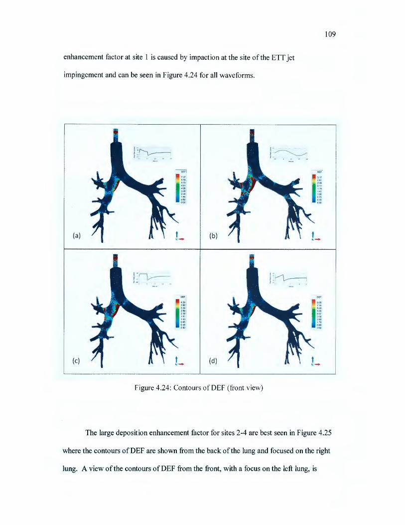
enhancement factor at site 1 is caused by impaction at the site of the ETT jet
impingement and can be seen in Figure 4.24 for all waveforms.
(a)
(c)
i:~ I « •• .. "
; «'1,---l ~. . " ..
737 6116 573 491 409 328 2 46 164 062 000
DEF '
4 20 382 334 286 239 191 143 095 0 48 000
(b)
(d)
Figure 4.24: Contours of DEF (front view)
1·· ,·~ 1 .
l : ........--, s« - v--l · • ' .
DEF
317 281 2•& 211 176 141 106 0 70 035 000
DEF
8.05 715 626 536 .. , 358 268 179 OU 000
109
The large deposition enhancement factor for sites 2-4 are best seen in Figure 4.25
where the contours of DEF are shown from the back of the lung and focused on the right
lung. A view of the contours of DEF from the front, with a focus on the left lung, is
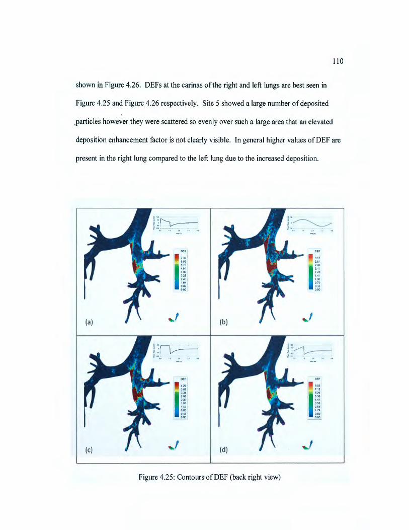
110
shown in Figure 4.26. DEFs at the carinas of the right and left lungs are best seen in
Figure 4.25 and Figure 4.26 respectively. Site5 showed a large number of deposited
,particles however they were scattered so evenly over such a large area that an elevated
deposition enhancement factor is not clearly visible. In general higher values of DEF are
present in the right lung compared to the left lung due to the increased deposition.
DEF DEF
7.37 3.17 6.55 2.81 5.73 246 4.91 211 4.09 1 76 3.28 1.41 2.46 1.06 1.64 070 0.82 0.35 0.00 000
DEF DEF
4 29 8.05 3.82 7.15 3.34 626 2.86 5.36 2.39 447 191 358 1.43 2.68 095 1.79 0.48 0.89 0.00 ~
Figure 4.25: Contours of DEF (back right view)

111
The differences in DEF between the key deposition sites are more pronounced for
the pressure controlled constant and flow controlled ascending ramp waveforms than the
pressure controlled sinusoidal or volume controlled ascending ramp waveforms. This
occurs because, at higher flow rates, there are more particles depositing at the lower
numbered sites and this leaves a smaller number of particles left to deposit at the higher
number sites. At lower flow rates the selection of particles reaching the different
deposition sites are more similar.
DEF
7.37 6.55 5.73 4.91 4.09 3.28 2 .46 1.64 0.82 0 .00
DEF
4.29 3.82 3.34 2.86 2.39 1.91 1.43 0 .95 0.48 0 .00
Figure 4.26: Contours of DEF (front left view)
DEF
3.17 2.81 2.46 2.11 1.76 1.41 1.06 0.70 0.35 0.00
8.05 7.15 6.26 5.36 4 .47 3.58 2.68 1.79 0.89 0.00
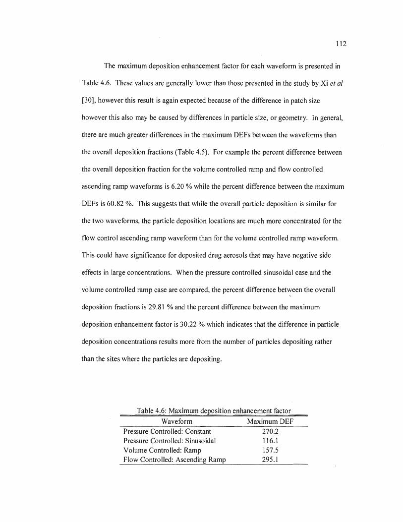
112
The maximum deposition enhancement factor for each waveform is presented in
Table 4.6. These values are generally lower than those presented in the study by Xi et al
[30], however this result is again expected because of the difference in patch size
however this also may be caused by differences in particle size, or geometry. In general,
there are much greater differences in the maximum DEFs between the waveforms than
the overall deposition fractions (Table 4.5). For example the percent difference between
the overall deposition fraction for the volume controlled ramp and flow controlled
ascending ramp waveforms is 6.20 % while the percent difference between the maximum
DEFs is 60.82 %. This suggests that while the overall particle deposition is similar for
the two waveforms, the particle deposition locations are much more concentrated for the
flow control ascending ramp waveform than for the volume controlled ramp waveform.
This could have significance for deposited drug aerosols that may have negative side
effects in large concentrations. When the pressure controlled sinusoidal case and the
volume controlled ramp case are compared, the percent difference between the overall
deposition fractions is 29.81 % and the percent difference between the maximum
deposition enhancement factor is 30.22 % which indicates that the difference in particle
deposition concentrations results more from the number of particles depositing rather
than the sites where the particles are depositing.
Table 4.6: Maximum deposition enhancement factor
Waveform Maximum DEF
Pressure Controlled: Constant 270.2 Pressure Controlled: Sinusoidal 116.1 Volume Controlled: Ramp 157.5 Flow Controlled: Ascending Ramp 295.1

113
5. CONCLUSIONS AND FUTURE WORK
In this study, a computational domain was reconstructed from CT scans of a 57
year old male patient undergoing mechanical ventilation treatment. A numerical model
was selected with appropriate boundary conditions and turbulence modeling using LES to
simulate fluid flow with a transient inlet boundary condition. Studies were performed to
ensure spatial and temporal convergence and simulations were run to validate the
numerical model with comparison to experimental data of Lieber and Zhao [ 117].
Computational fluid dynamics along with a user defined particle force subroutine were
applied to evaluate fluid flow and particle deposition characteristics for flow in the upper
tracheobronchial region for a range of inspiratory waveforms typically seen in patients
undergoing mechanical ventilation treatment.
5.1. CONCLUSIONS
From the evaluation of the fluid flow it was clear that the jet caused by the
endotracheal tube was an important fluid flow feature with effects similar to that of the
laryngeal jet. These effects include: high flow rates in the trachea, the creation of a zone
ofrecirculation, the initiation of turbulence, and the impaction of particles at the site of
the jet's impingement. The full range of effects of the jet caused by the endotracheal tube
is not fully understood and requires further study. The presence and strength of the
recirculation zone in the right main bronchus and the swirling flows in the bronchi were
found to be dependent upon the flow history as well as the inspiratory flow rate. This
implies that these transient fluid flow events may not be captured with steady state
analyses. Strong turbulence was found in the wake of the jet caused by the flow from the
endotracheal tube which dissipated in the lower airways of the domain as indicated by
vorticity magnitude and turbulence kinetic energy.
114
From the evaluation of particle deposition within the tracheobronchial model, it
was found that particle impaction was linked to inspiratory flow rate with the rate of
particle deposition generally following the inspiratory flow rate. The lowest value of
overall deposition fraction was found in the pressure controlled sinusoidal waveform,
followed by the volume controlled ramp, pressure controlled constant, and flow
controlled ascending ramp with the highest overall deposition fraction. This does not_
create implications on particle deposition in the lower airways that were not included in
the domain.
Upon evaluation of the local deposition, several key deposition locations were
identified including: the site of impingement and deflection of the jet caused by the
endotracheal tube on the wall of the right main bronchus, the site where the deflected jet
impinges on the wall of the right main bronchus, the walls surrounding the large rotating
structure in the right main bronchus, the superior wall of the branch leading to the right
upper lobe, the superior wall of the left main bronchi near the first bifurcation, and the
carinas of the airway bifurcations. The size of the particles depositing at the key
deposition locations is linked with peak inspiratory flow rate due to the effects of particle
impaction, turbulent dispersion and turbophoresis. The time at which particles deposit is
also typically matched with the time of peak inspiratory flow. Finally the differences in
the deposition enhancement factors and the overall deposition fractions give evidence of
drug aerosol concentrations in key deposition sites which may be significant for drugs
with negative side effects in high concentrations.

5.2. FUTURE WORK
For numerical studies to be clinically applicable, a degree of realism must be
represented by the complete numerical model including the geometry, boundary
conditions, and treatment of turbulence [13]. The current work studies fluid flow and
particle deposition in a reconstructed model for a single intubated patient with a
proportional mass flow rate outlet condition. Future work on fluid flow and particle
transport in the human respiratory system may include the following:
115
• Detailed study of the endotracheal tube: The results of this study combine_d
with the lack of detailed work on the endotracheal tube, show a need for studies to
investigate the effects of endotracheal tube characteristics on fluid flow and particle
deposition. A study performed by Esteban et al [37] reports that 99 % of the patients
studied undergoing mechanical ventilation in America were ventilated through intubation
or a tracheostomy. This indicates that a better understanding of the effects of the
endotracheal tube is critical for clinical applications. Studies will be performed to
investigate the effects of endotracheal tube size and position on fluid flow and particle
deposition for patients undergoing mechanical ventilation treatment.
• Improving the outlet condition: An outlet condition based on a proportional
mass flow rate has been applied by studies in the past; however an alternate outlet
condition may be more physiologically realistic [30, 70, 115-116, 128]. Results that are
more physiologically realistic may be achieved with a boundary condition that models the
outlets as balloons with flow resistance. The pressure at each outlet could be specified
based on the volume of flow that has passed through the outlet and the instantaneous flow
rate combined with data of airway compliance and resistance.

116
• Patient specific studies: The use of geometry based on the CT scans of patients
helps to ensure a realistic geometry and is an important step towards clinical usefulness
[13]. However conclusions drawn from the results of simulations in the airways ofa
single patient may not be representative of the airways of every patient. In order to
provide useful insight into fluid flow and aerosol drug delivery for clinicians it is
important to consider patient specific geometry and boundary conditions [128]. Further
study is necessary to determine what patient to patient differences will significantly
impact drug aerosol delivery. In addition further techniques must be developed to
measure and account for these significant patient to patient differences.
• Experimental work: CFD has proven useful in evaluating fluid flow and
particle deposition in simplified numerical models of the human airways. To make these
CFD studies more useful for real world applications the complexity of the numerical
models must grow. With the growth of complexity of numerical models it becomes
increasingly important to validate these numerical methods with experimental results.
Experiments will be carried out to further validate the numerical methods used in the
present and future works.
APPENDIX A.
VALIDATION AND CONVERGENCE STUDY GEOMETRY CREATION
CODE
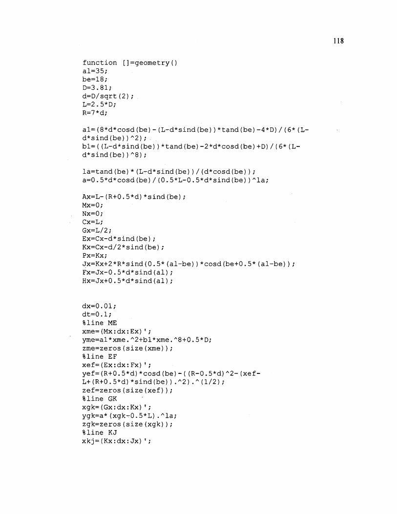
function []=geometry() al=35; be=18; 0=3.81; d=O/sqrt(2); 1=2.5*0; R=7*d;
al=(8*d*cosd(be)-(L-d*sind(be))*tand(be)-4*0)/(6*(1-d*sind(be))A2); . bl=((L-d*sind(be))*tand(be)-2*d*cosd(be)+0)/(6*(Ld*sind(be))A8);
la=tand(be)*(L~d*sind{be))/(d*cosd(be)); a=O.S*d*cosd(be)/(O.S*L-0.S*d*sind(be))Ala;
Ax=L-(R+O.S*d)*sind(be); Mx=O; Nx=O; Cx=L; Gx=L/2; Ex=Cx-d*sind(be); Kx=Cx-d/2*sind(be); Px=Kx; ~x=Kx+2*R*sind(0.5*(al-be))*cosd(be+0.5*(al-be)); Fx=Jx-0.S*d*sind(al); Hx=Jx+O.S*d*sind(al);
dx=0.01; dt=0.1; %line ME. xme=(Mx:dx:Ex) '; yme=al*xme.A2+bl*xme.A8+0.5*0; zme=zeros(size(xme)); %line EF xef= (Ex: dx: Fx) '; yef=(R+O.S*d)*cosd(be)-((R-0.S*d)A2-(xefL+(R+O.S*d)*sind(be)) .A2) .A(l/2); zef=zeros(size(xef)); %line ·GK xgk=(Gx:dx:Kx) '; ygk=a*(xgk~0.5*1) .Ala; zgk=zeros(size(xgk)); %line KJ xkj=(Kx:dx:Jx) ';
118
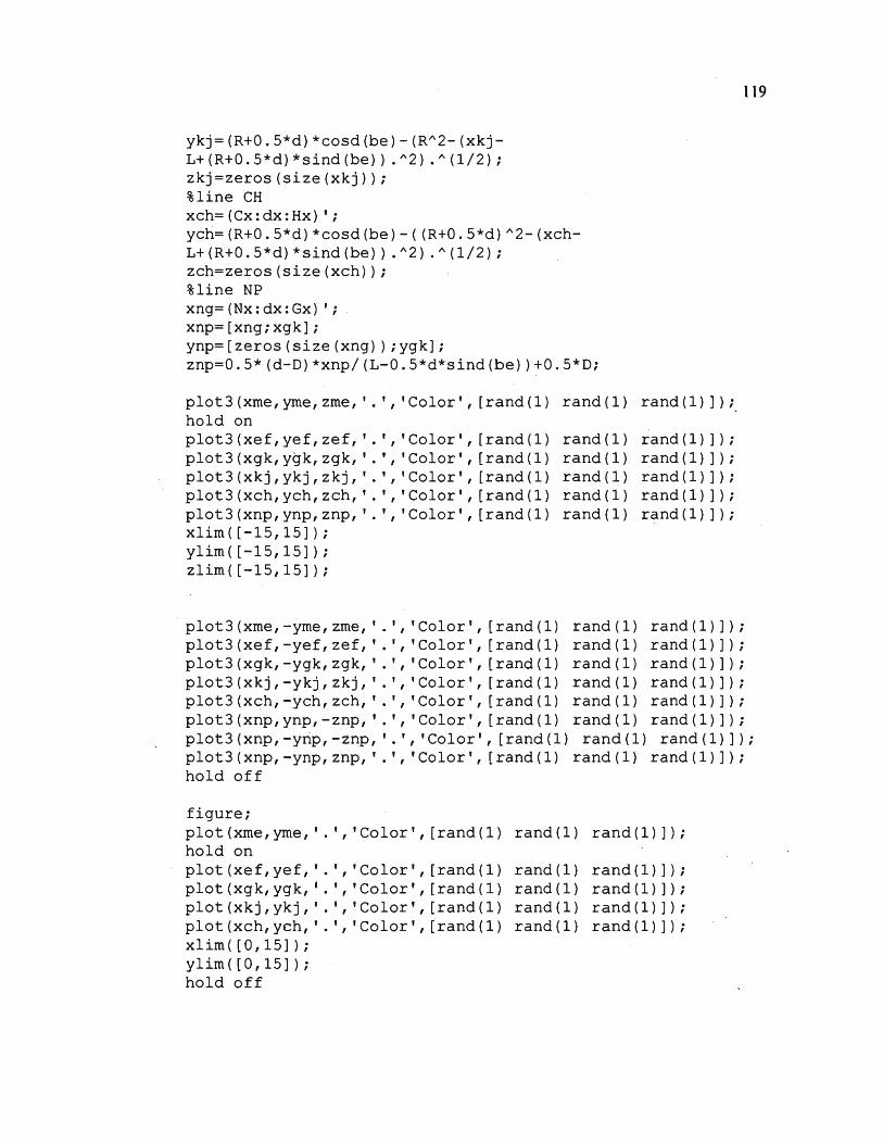
ykj=(R+0.5*d)*cosd(be)-(RA2-(xkjL+(R+0.5*d)*sind(be)) .A2) .A(l/2); zkj=zeros(size(xkj)); %line CH xch= (Cx:dx:Hx) '; ych=(R+0.5*d)*cosd(be)-((R+0.5*d)A2-(xchL+ (R+O. 5*d) *sind (be)) . A2). A ( 1/2); zch=zeros(size(xch)); %line NP xng=(Nx:dx:Gx) '; xnp=[xng;xgk]; ynp=[zeros(size(xng)) ;ygk]; znp=0.5*(d-D)*xnp/(L-0.5*d*sind(be))+0.5*D;
plot3(xme,yme,zme, '.','Color', [rand(l) rand(l) rand(l) ])?. hold on plot3(xef,yef,zef, '.','Color', [rand(l) rand(l) rand(l)]); plot3(xgk,ygk,zgk, '.','Color', [rand(l) rand(l) rand(l)]); plot3 (xkj, ykj, zkj, '. ', 'Color', [rand ( 1) rand ( 1) rand ( 1)]); plot3(xch,ych,zch, '.','Color', [rand(l) rand(l) rand(l)]); plot3(xnp,ynp,znp, '.','Color', [rand(l) rand(l) rand(l)]); x1 im ( [ -15 , 15 ] ) ; y 1 im ( [ - 15 , 15 ] ) ; z 1 im ( [ -15 , 15 ] ) ;
119
plot3(xme,-yme,zme,' .', 'Color', [rand(l) rand(l) rand(l)]); plot3 (xef, -yef, zef, ' . ', 'Color', [ rand ( 1) rand ( 1) rand ( 1) ] ) ; plot3(xgk,-ygk,zgk, '.', 'Color', [rand(l) rand(l) rand(l)]); plot3 (xkj, -ykj, zkj, ' . ', 'Color', [ rand ( 1) rand ( 1) rand ( 1)] ) ; plot3(xch,~ych,zch, '.', 'Color', [rand(l) rand(l) rand(l)]); plot3(xnp,ynp,-znp, '.','Color', [rand(l) rand(l) rand(l)]); plot3(xnp,-yrip,-znp, '.','Color', [rand(l) rand(l) rand(l)]); plot3 ( xnp, -ynp, znp, ' . ' , 'Color' , [ rand ( 1) rand ( 1) rand ( 1) ] ) ; hold off
figure; plot(xme,yme,'. ', 'Color', [rand(l) rand(l) rand(l)]); hold on plot(xef,yef,'. ', 'Color', [rand(l) rand(l) rand(l)]); plot(xgk,ygk,'. ', 'Color', [rand(l) rand(l) rand(l)]); plot(xkj,ykj,' .', 'Color',[rand(l) rand(l) rand(l)]); plot(xch,ych,'. ', 'Color', [rand(l) rand(l) rand(l)]); x 1 im ( [ 0 , 1 5 ] ) ; y 1 im ( [ 0 , 15 ] ) ; hold off

xmef=[xme;xef]; ymef=[yme;yef]; zmef= [ zme; zef] ; file=fopen('curveMEF.txt', 'wt'); for i=l:length(xmef)
fprintf(file, '%1.Sf %1.Sf %1.8f\n',xmef(i),ymef(i),zmef(i) ); end fclose(file);
xgkj=[xgk;xkj]; ygkj=[ygk;ykj]; zgkj=[zgk;zkj]; file=fopen('curveGKJ.txt', 'wt'); for i=l:length(xgkj)
fprintf(file, '%1.Sf %1.Sf % 1. 8 f\n' , xgkj ( i) , ygkj ( i) , zgkj ( i) ) ; end f close (file) ;
file=fopen('curveCH.txt', 'wt'); for i=l:length(xch)
fprintf(file, '%1.Sf %1.Sf ~1. 8f\n', xch (i), ych (i), zch (i)); end f close (file) ;
xnpkj=[xnp;xkj]; ynpkj=[ynp;ykj]; znpkj=[znp;zkj+d/2]; file=fopen('curveNPKJl.txt', 'wt'); for i=l:length(xnpkj)
fprintf(file, '%1.Sf %1.Sf %1.Sf\n',xnpkj (i),ynpkj (i),znpkj(i) ); end fclose(file);
xnpkj=[xnp;xkj]; ynpkj=[-ynp;-ykj]; znpkj=[znp;zkj+d/2]; file=fopen('curveNPKJ2.txt', 'wt'); for i=l:length(xnpkj)
fprintf(file, '%1.Sf %1.Sf %1.Sf\n',xnpkj (i),ynpkj (i),znpkj(i)); end fclose(file);
120

xnpkj=[xnp;xkj]; ynpkj=[ynp;ykj]; znpkj=I-znp;-(zkj+d/2)]; file=fopen('curveNPKJ3.txt', 'wt'); foi i=l:length(xnpkj)
fprintf(file, '%1.8f %1.8f %1.8f\n',xnpkj(i),ynpkj (i),znpkj (i)); end fclose(file);
xnpkj=[xnp;xkj]; ynpkj=[-ynp;-ykj]; znpkj=[-znp;-(zkj+d/2)]; file=fopen('curveNPKJ4.txt', 'wt'); for i=l:length(xnpkj)
fprintf(file, '%1.8f %1.8f %1.8f\n',xnpkj (i),ynpkj (i),znpkj (i)); end fclose(file);
function []=pr(xl,dx,th,yl,wh) al=35; be=18; 0=3.81; d=O/sqrt(2); 1=2.5*0; R=7*d; a1=(8*d*cosd(be)-(L-d*sind(be))*tand(be)-4*0)/(6*(1-d*sind(be))"'2); bl=( (L-d*sind(be))*tand(be)-2*d*cosd(be)+0)/(6*(Ld*sind(be))"'8); la=tand(be)*(L-d*sind(be))/(d*cosd(be)); a=0.5*d*cosd(be)/(0.5*1-0.5*d*sind(be))"'la; psl=(xl(l) :dx:xl(2)) '; ps2=(xl(l) :dx:xl(2)) '; y=L/2*tand(be)-psl.*cosd(th)-al.*(L/2+psl.*sind(th)) ."'2-bl.*(L/2+psl.*sind(th)) ."'8-0.5*0; %w=~ cosd(th) - 2*al*sind(th)*(L/2 + psl*sind(th)) -S*bl*sind(th)*(L/2 + psl*sind(th)) ."'7; z=L/2*tand(beY-ps2.*cosd(th)-a.*(ps2.*sind(th)) ."'(la); w=- cosd(th) - a*la*sind(th)*(ps2*sind(th)) ."'(la - 1); if (wh==O)
plot(psl,z); elseif(wh==l)
plot (psl, w); elseif(wh==2)
121

plot(psl,z,psl,w); end if (yl)
y 1 im ( [ - . 1, . 1] ) ; end
function [y]=psleq(th,psl) be=l8; 0=3.81; d=D/sqrt(2); 1=2.S*D; a1=(8*d*cosd(be)-(L-d*sind(be))*tand(be)-4*0)/(6*(Ld*sind(be))"2); bl=((L-d*sind(be))*tand(be)-2*d*cosd(be)+D)/(6*(Ld*sind(be))"8); y=L/2*tand(be)-psl.*cosd(th)-al.*(L/2+psl.*sind(th)) ."2- · bl.* (L/2+psl. *sind (th)) . "8-0. S*D;
function [y]=ps2eq(th,ps2) be=l8; 0=3.81; d=D/sqrt(2); 1=2.S*D; la=tand(be)*(L-d*sind(be))/(d*cosd(be)); a=0.5*d*cosd(be)/(0.5*L-0.5*d*sind(be) )"la; y=L/2*tand(be)-ps2.*cosd(th)-a.*(ps2.*sind(th)l."(la);
122
APPENDIXB.
WOMERSLEY VELOCIY PROFILE SUBROUTINE
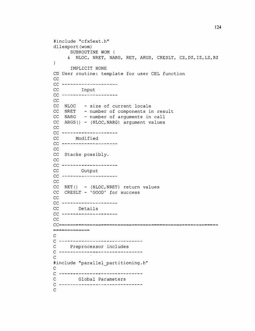
#include "cfx5ext.h" dllexport(wom)
SUBROUTINE WOM
124
& NLOC, NRET, NARG, RET, ARGS, CREStT, CZ,DZ,IZ,LZ,RZ
IMPLICIT NONE CD User routine: template for user CEL function cc cc--------------------cc Input cc--------------------cc CC NLOC - size of current locale CC NRET - number of components in result CC NARG - number of arguments in call CC ARGS() - (NLOC,NARG) argument values cc cc--------------------cc Modified cc--------------------cc CC Stacks possibly. cc cc--------------------cc Output cc--------------------cc CC RET() - (NLOC,NRET) return values CC CRESLT - 'GOOD' for success cc cc--------------------cc Details cc--------------------cc CC=========================================================
c c ------------------------------c Preprocessor includes c ------------------------------c #include "parallel_partitioning.h" c c ------------------------------c Global Parameters c ------------------------------c

c c ------------------------------c Argument list c ------------------------------c
c
c
c
c
INTEGER NLOC,NARG,NRET
CHARACTER CRESLT*(*)
REAL ARGS(NLOC,NARG), RET(NLOC,NRET)
INTEGER IZ(*) CHARACTER CZ(*)*(l) DOUBLE PRECISION DZ(*) LOGICAL LZ(*) REAL RZ(*)
c ------------------------------c External routines c ------------------------------c c c ------------------------------c Local Parameters c ------------------------------
COMPLEX I PARAMETER(I=(O,l))
c ------------------------------c Local Variables c ------------------------------c
c
INTEGER ILOC REAL AL(l:NLOC,l), R(l:NLOC,l), T(l:NLOC,l),
& A(l:NLOC,l), W(l:NLOC,l), P(l:NLOC,l) COMPLEX B, C
c ------------------------------c Stack pointers c ------------------------------c
125
C==========================================================
c c ---------------------------c Executable Statements c ---------------------------c

c
R(l:NLOC,1) ARGS(l:NLOC,l) T(l:NLOC,l) ARGS(l:NLOC,2) A(l:NLOC,l) ARGS(l:NLOC,3) W(l:NLOC,l) ARGS(l:NLOC,4) P(l:NLOC,l) ARGS(l:NLOC,5) AL(l:NLOC,1) = ARGS(l:NLOC,6)
C Initialise RET(l:NLOC*NRET) to zero. c
DO ILOC = 1, NLOC CALL CBESSJ(COMPLEX(AL(ILOC,1)*
& R(ILOC,1)/0.01905,0.)*(I**(3./2.)),0,B) CALL
CBESSJ(COMPLEX(AL(ILOC,1),0.)*(I**(3./2.) ),0,C) B=(COMPLEX(A(ILOC,1)/(P(ILOC,l)*W(ILOC,1) ),0.)/I)
& *(COMPLEX(l.0,0.)-B/C)*EXP(I*COMPLEX(W(ILOC,l)
c
& *(T(ILOC,1)+18.0238016767),0.)) RET(ILOC,l)=REAL(B)
END DO
C Set success flag. CRESLT = 'GOOD'
c
126
C==========================================================
c
c
END SUBROUTINE WOM
real*B Function Fact(K) integer i real*B f
F=l.dO do i=2, k
f=f*dfloat(i) end do Fact=f
return End Function Fact
*******************************************
* FUNCTION GAMMA(X) [129] * * --------------------------------------- * * Returns the value of Gamma(x) in double* * precision as EXP(LN(GAMMA(X) )) for X>O. * *******************************************
real*B Function Gamma(xx) parameter(ONE=l.d0,FPF=5.5d0,HALF=0.5d0)
real*B xx
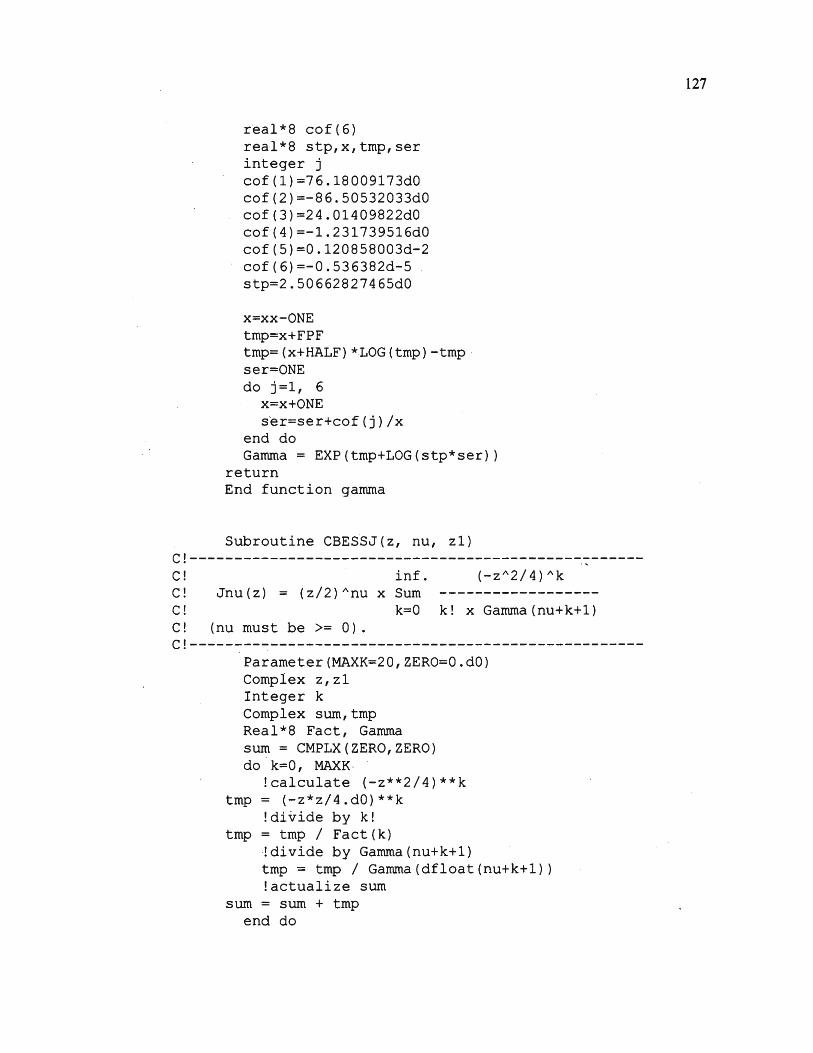
real*8 cof(6) real*8 stp,x,tmp,ser integer j cof(l)=76.18009173d0 cof(2)=-86.50532033d0 cof(3)=24.01409822d0 cof(4)=-l.231739516d0 cof(5)=0.120858003d-2 cof(6)=-0.536382d-5 stp=2.50662827465d0
x=xx-ONE tmp=x+FPF tmp=(x+HALF)*LOG(tmp)-tmp · ser=ONE do j=l, 6
x=x+ONE ser=ser+cof(j)/x
end do Ganuna = EXP(tmp+LOG(stp*ser))
return End function gamma
Subroutine CBESSJ(z, nu, zl) C!-------------------- ---------------------- .. ------C! inf. (-zA2/4)Ak C! Jnu(z) = (z/2)Anu x Sum ------------------Cl k=O kl x Gamma(nu+k+l) Cl (nu must be>= 0). C!---------------------------------------------------
Parameter(MAXK=20,ZERO=O.d0) Complex z,zl Integer k Complex sum,tmp Real*8 Fact, Gamma sum= CMPLX(ZERO,ZERO) do k=O, MAXK-
! calculate (-z**2/4)**k tmp = (-z*z/4.dO)**k
!divide by k! tmp = tmp I Fact(k)
·!divide by Gamma(nu+k+l) tmp = tmp I Gamma(dfloat(nu+k+l)) !actualize sum
sum= sum+ tmp end do
127

tcalculate (z/2)**nu tmp = (z/2)**nu !multiply (z/2)**nu by sum zl = tmp*sum
return End
C!end of file wom.F
128

APPENDIX C.
WAVEFORM GENERATION CODES
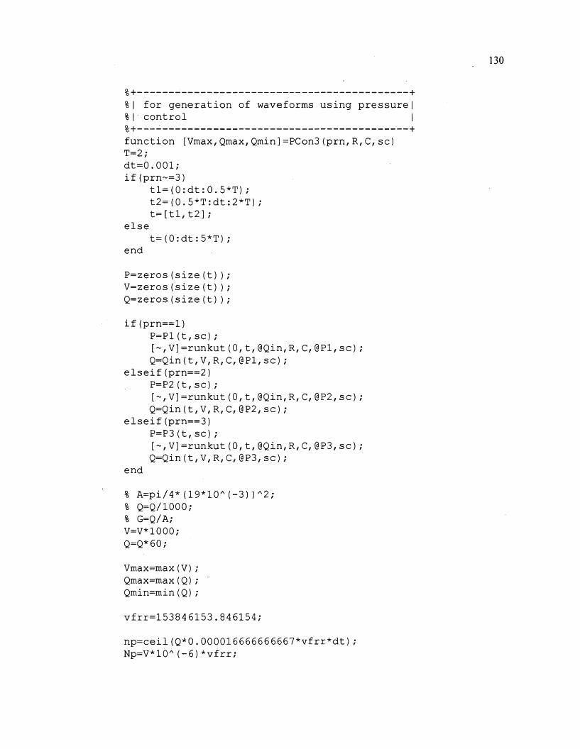
%+------ ·------------------------------------+ %1 for generation of waveforms using pressure! %1· control I %+--- ·----------------------------- ---------+ function [Vmax,Qmax,Qmin]=PCon3(prn,R,C,sc) T=2; dt=0.001; if(prn-=3)
tl=(O:dt:0.5*T); t2=(0.5*T:dt!2*T); t=[tl,t2];
else t=(O:dt:5*T);
end
P=zeros(size(t) ); V=zeros(size(t) ); Q=zeros(size(t) );
if (prn==l) P=Pl(t,sc); [-,V]=runkut(O,t,@Qin,R,C,@Pl,sc); Q=Qin(t,V,R,C,@Pl,sc);
elseif(prn==2) P=P2(t,sc); [-,V]=runkut(O,t,@Qin,R,C,@P2,sc); Q=Qin(t,V,R,C,@P2,sc);
elseif(prn==3)
end
P=P3(t,sc); [-,V]=runkut(O,t,@Qin,R,C,@P3,sc); Q=Qin(t,V,R,C,@P3,sc);
% A=pi/4*(19*10A(-3))A2; % Q=Q/1000; % G=Q/A; V=V*lOOO; Q=Q*60;
Vmax=max (V) ; Qmax=max(Q); Qmin=min ( Q) ;
vfrr=l53846153.846154;
np=ceil(Q*0.000016666666667*vfrr*dt); Np=V*l0A(-6)*vfrr;
130
disp(sum(np(l:ceil(length(np)*l.042/4) ))); disp(ceil(length(np)*l.042/4) );
po= I b Ii subplot(3,1,1); plot(t,P,po); title('Pressure'); xlabel('time(s) '); ylabel('Pressure .(cm H_20) '); subplot(3,1,2); plot(t,V,po); title('Volume'); xlabel('time(s) '); ylabel('Volume(mL) '); subplot(3,1,3); plot(t,Q,po); title ('Flow' ) ; xlabel('time(s) '); ylabel('Flow(L/min) ');
disp(V(end));
Ain=pi/4*(8.35868*10A(-3))A2;%pi/4*(16.4E-3)A2; K=Q/60/1000/Ain;
figure; plot(t,Np, 'b. ');
filename=strcat('pr',num2str(prn), '.csv'); file=fopen(filename, 'wt'); fprintf(file,' [name]\ninlet\n\n[Spatial Fields]\nt\n\n[Data]\nt [s],Velocity [m sA-1]\n'); for i=l:length(t)
fprintf(file, '%1.6E,%1.6E\n',t(i),K(i)); end fclose(file);
filename=strcat ( 'Npr', num2str (prn), ' . csv'); file=fopen(filename, 'wt'); fprintf (file, ·, [name] \nRealPartNum\n\n [Spatial Fields]\nt\n\n[Data]\nt [s],NPR []\n'); for i=l:length(tl)
fprintf(file, '%1.6E,%1.6E\n',t(i),Np(i)); end fclose(file);
131

%definition of pressure curve function [z]=Pl(t,sc) z=sc*ones(size(t)) .*sig(t) .*rsig(t,1);
function [z]=P2(t,sc) z=sc*(l-exp(-4*t)) .*rsig(t,1);
function [z]=P3(t,sc) z=sc/3*(1-cos(2*pi*t));
function [z]=sig(t) td=0.1; z=(l/2-1/2*cos(t*pi/td)) .*(1-heaviside(ttd) )+l*heaviside(t-td);
function [z]=rsig(t,s) td=0.1; z=(l/2-1/2*cos((t-s)*pi/td+pi)) .*(heaviside(t-s)) .*(1-heaviside(t-(s+td)) )+(1-heaviside(t-s));
%differential equation function [Vdot]=Qin(t,V,R,C,Pr,sc) Vdot=Pr(t,sc)/R-V/(C*R);
%+-------------------------------------------+ %1 for generation of waveforms using volume I %1 control I %+----- -------------------------------------+ function [Vmax,Qmax,Qmin]=VCon3(von,R,C,sc) T=2; dt=0.001; tl=(O:dt:O.S*T); t2=(0.S*T:dt:2*T); t=[tl,t2];
P=zeros(size(t)); V=zeros(size(t)); Q=zeros(size(t) );
if(von==l) V(l:length(tl))=Vl(tl,sc); for i=l:length(tl)-1
Q(i)=( (V(i+l)-V(i) )/(tl(i+l)-tl(i)) )*sig(tl(i) );
132
133
end · Q(length(tl) )=(V(length(tl))-V(length(tl)-1))/(tl(end)
tl .(end-l) ); V(l)=O; for i=2:length(tl)
V(i)=V(i-l)+(Q(i)+Q(i-l))*(tl(i)-tl(i-1))/2; end
elseif(von==2) V(l:length(tl))=V2(tl,sc); for i=l:length(tl)-1
Q(i)=(V(i+l)-V(i))/(tl(i+l)-tl(i)); end Q(length(tl) )=(V(length(tl))-V(length(tl)-1))/(tl(end)
tl(end-1) ); end
P(l:length(tl))=Q(l:length(tl))*R+V(l:length(tl))/C;
P(length(tl)+l:length(t))=Pr(t2,P(length(tl)) ); [-,V(length(tl)+l:length(t)) ]=runkut(V(length(tl) ),t2,@Qout ,R,C,@Pr,P(length(tl) )); Q(length(tl)+l:length(t) )=Qout(t2,V(length(tl)+l:length(t)) ,R,C,@Pr,P(length(tl)));
% P(length(tl)+l:length(t))=Pr(t2,P(length(tl))); % . ,
[-,V(length(tl)+l:length(t))]=runkut(V(length(tl) ),t2,@Qout ,R,C,@Pr,P(length(tl))); % Q(length(tl)+l:length(t) )=Qout(t2,V(length(tl)+l:length(t)) ,R,C,@Pr,P(length(tl)));
V=V*lOOO; Q=Q*60;
Vrnax=rnax(V); Qrnax=rnax(Q); Qrnin=rnin(Q);
vfrr=l53846153.846154;
np=ceil(Q*0.000016666666667*vfrr*dt); Np=V*10A(-6)*vfrr;
disp(surn(np(l:ceil(length(np)*l.042/4))) ); disp(ceil(length(np)*l.042/4));

% P=P/98. 0665; % V=V*lOOO*lOOO; % Q=Q*60000;
po='b'; subplot(3, 1, 1); plot(t,P,po}; title('Pressure'); xlabel('time(s) '); ylabel('Pressure(cm H_20) '); subplot(3,1,2); plot(t,V,po); tit 1 e ( ' Vo 1 ume ' ) ; xlabel('time(s) '); ylabel('Volume(mL) '); subplot(3,1,3); plot(t,Q,po); title ('Flow ·'); xlabel('time(s) '); ylabel('Flow(L/min) ');
Ain=pi/4*(8.35868*1QA(-3))A2; K=Q/60/1000/Ain;
figure; plot ( t, Np, 'b. ' ) ;
filename=strcat('vo',num2str(von), '.csv'); file=fopen(filename, 'wt'); fprintf(file,' [name]\ninlet\n\n[Spatial Fields]\nt\n\n[Data]\nt [s],Velocity [m sA-1]\n'); , for i=l:length(t)
fprintf(file,'%1.6E,%1.6E\n',t(i),K(i)); end fclose(file);
filename=strcat('Nvo',num2str(von), '.csv'); file=fopen(filename, 'wt'); fprintf(file,' [name]\nRealPartNum\n\n[Spatial Fields]\nt\n\n[Data]\nt [s],NPR []\n'); for i=l: length'( tl)
fprintf(file, '%1.6E,%1.6E\n',t(i),Np(i)); end fclose(file);
%definition of volume curves function [z]=Vl(t,sc)
134
z=sc*10A(-3)*0.9927*t;
function [z]=V2(t,sc) z=sc*10A(-3)*(1/2-1/2*cos(pi*t));
function [z]=sig(t) td=0.1; z=(l/2-1/2*cos(t*pi/td)) .*(1-heaviside(ttd) )+l*heaviside(t-td);
function [z]=rsig(t,s) td=0.1; z=(l/2-1/2*cos( (t-s)*pi/td+pi)) .*(heaviside(t-s)) .*(1-heaviside(t-(s+td)))+(l-heaviside(t-s));
function [z]=Pr(t,p) z=p*rsig(t,1);
%differential equation function [Vdot]=Qout(t,V,R,C,Pr,s) Vdot=Pr(t,s)/R-V/(C*R);
%+-------------------------------------------+ %1 for generation of waveforms using flow I % I control 1 .. %+-------------------------------------------+ function [Vmax,Qmax,Qmin]=QCon3(Qn,R,C,sc) T=2; dt=0.001; tl=(O:dt:O.S*T); t2=(0.5*T:dt:2*T); t=[tl,t2];
P=zeros(size(t) ); V=zeros(size(t) ); Q=zeros(size(t) );
if (Qn==3) t=(O:dt:2*T); tl=(O:dt:T); t2= (T:dt: 2*T); V=zeros(size(t)); Q=Q3(t,sc); V(l)=O; for i=2:length(t)
V(i)=V(i-l)+(Q(i)+Q(i-l))*(t(i)-t(i-1))/2;
135

else
end P=Q*R+V/C;
if (Qn==l) Q(l:length(tl))=Ql(tl,sc);
elseif(Qn==2} Q(l:length(tl))=Q2(tl,sc);
end V(l)=O; for i=2:length(tl)
V(i)=V{i-l)+(Q(i)+Q(i-l))*(tl(i)-tl(i-1))/2; end
136
P(l:length(tl))=Q(l:length(tl))*R+V(l:length(tl) )/C; P(length(tl)+l:length(t) )=Pr(t2,P(length(tl))); [-,V(length(tl)+l:length(t)) ]=runkut(V(length(tl)),t2,@Q?ut ,R,C,@Pr,P(length(tl))); Q(length(tl)+l:length(t) )=Qout(t2,V(length(tl)+i:length(t)) ,R,C,@Pr,P(length(tl))); end
V=V*lOOO; Q=Q*60;
Vmax=max (V) ; Qmax=max(Q); Qmin=min(Q);
vfrr=153846153.846154;
np=ceil(Q*0.000016666666667*vfrr*dt); Np=V*10A(-6)*vfrr;
disp(sum(np(l:ceil(length(np)*l.042/4)) )); disp(ceil(length(np)*l.042/4));
% P=P/98.0665; % V=V*lOOO*lOOO; % Q=Q*60000;
po= I b Ii subplot(3,l,1); plot(t,P,po); title('Pressure'); xlabel('time(s) '); ylabel('Pressure(cm H_20) '); subplot(3,1,2); plot(t,V,po);

title ('Volume'); xlabel('time(s) '); ylabel('Volume(mL) '); subplot(3,1,3); plot(t,Q,po); title ('Flow'); xlabel ( 'time ( s) ' ) ; ylabel('Flow(L/min) ');
Ain=pi/4*(8.35868*10A(-3))A2; K=Q/60/1000/Ain;
figure; plot(t,Np, 'b. ');
filename=strcat('Q',num2str(Qn), '.csv'); file=fopen(filename, 'wt'); fprintf(file,' [name]\ninlet\n\n[Spatial Fields]\nt\n\n[Data]\nt [s],Velocity [m sA-1]\n'); for i=l:length(t)
fprintf(file, '%1.6E,%1.6E\n',t(i),K(i) ); end fclose(file);
filename=strcat('Nq',num2str(Qn), '.csv'); file=fopen(filename, 'wt'); fprintf(file,' [name]\nRealPartNum\n\n[Spatial Fields]\nt\n\n[Data]\nt [s],NPR []\n'); for i=l:length(tl)
fprintf(file, '%1.6E,%1.6E\n',t(i),Np(i)); end fclose(file);
%definition of flow rate curves function [z]=Ql(t,sc) z=sc*0.9808*(2*t);
function [Z]=Q2(t,sc) z=sc*(2-2*t) .*sig(t);
function [z]=Q3(t,sc) z=sc*sin(2/4*pi*t);
function [z]=sig(t) td=0.1; z=(l/2-1/2*cos(t*pi/td)) .*(1-heaviside(ttd) )+l*heaviside(t-td);
137
function [z]=rsig(t,s) td=0.1; z=(l/2-1/2*cos( (t-s)*pi/td+pi)) .*(heaviside(t-s)) .*(1-heaviside(t-(s+td)) )+(1-heaviside(t-s));
function [z]=Pr(t,p) z=p*rsig(t,1);
%differential equation function [Vdot]=Qout(t,V,R,C,Pr,s) Vdot=Pr(t,s)/R-V/(C*R);
138
139
BIBLIOGRAPHY
1. Hickey, A.J., Pharmaceutical inhalation aerosol technology. Vol. 56. 1992, New York, NY: Marcel Dekker.
2. Dreyfuss, D. and G. Saumon, From Ventilator-Induced Lung Injury to Multiple Organ Dysfunction. Intensive Care Medicine, 1998. 24: p. 102-104.
3. Kleinstreuer, C. and Z. Zhang, Airflow and particle transport in the human respiratory system. Annual Review of Fluid Mechanics, 2009. 42: p. 301-334.
4. Levitzky, M.G., Pulmonary Physiology. 2003: McGraw-Hill ProefessionaL 278.
5. Hickey, A.J., Inhalation aerosols: physical and biological basis/or therapy:Vol. 94. 1996, New York, NY: Marcel Dekker.
6. Starr, C., C. Evers, and L. Starr, Biology: today and tomorrow: with physiology. 3 ed. 2009: Cengage Learning.
7. The Oropharynx and Hypopharynx. 03/12/2011 [cited 2012 03/19]; Available from: http://www.painneck.com/ompharynx-hypopharynx.
8. Horsfield, K., Models of the Human Bronchial Tree. Journal of Applied Physilology, 1971. 31(2): p. 207-217.
9. Weibel, E.R., Morphological Basis of Alveolar-Capillary Gas Exchange. Physiological Reviews, 1973. 53(2): p. 419-495.
10. Mobley, C. and G. Hochhaus, Methods used to assess pulmonary deposition and absorption of drugs. Drug Discovery Today, 2001. 6(7): p. 367-375.
11. White, F.M., Fluid Mechanics. 6 ed. 2008: McGraw-Hill Higher Education. 864.
12. Olson, D.E., et al., Convective Patterns of Flow Durrring Inspiration. Archives of Internal Medicine, 1973. 131: p. 51-57.
13. Kleinstreuer, C. and z. Zhang, Airflow and particle transport in the human respiratory system. Annual Review of Fluid Mechanics, 2010.·42: p. 301-334.
14. Kleinstreuer, C., Z. Zhang, and J.F. Donohue, Targeted Drug-Aerosol Delivery in the Human Respiratory System. Annual Review of Biomedical Engineering, 2008. 10: p. 195-220.
15. Bouhuys, A., Breathing; physiology, environment and lung disease. 1974: Grune & Stratton. 511.

16. Thurlbeck, W.M. and A. Churg, Pathology of the lung. 1995: Thieme Medical Publishers.
140
17. Weibel, E.R., Morphometry of the human lung. 1963, New York, NY: Academic.
18. Xia, G., et al., Airway Wall Stiffening Increases Peak Wall Shear Stress: A FluidStructure Interaction Study in Rigid and Compliant Airways. Annals of Biomedical Engineering, 2010. 38(5): p. 1836-1853.
19. Zhang, H. and G. Papadakis, Computational analysis of flow structure and particle deposition in a single asthmatic human airway bifurcation. Journal of Biomechanics, 2010. 43: p. 2453-2459.
20. Nagels, M.A. and J.E. Carter, Large eddy simulation of high frequency oscillating flow in an asymmetric branching airway model. Medical Engineering and Physics, 2009. 31: p. 1148-1153.
21. Comer, J.K., C. Kleinstreuer, and C.S. Kim, Flow structures and particle deposition patterns in double-bifurcation airway models. Part 2. Aerosol transport and deposition. Journal of Fluid Mechanics, 2001 b. 435: p. 55-80.
22. Comer, J.K., C. Kleinstreuer, and Z. Zhang, Flow structures and particle deposition patterns in double-bifurcation airway models. Part 1. Air flow fields. Journal of Fluid Mechanics, 200la. 435: p. 25-54.
23. Zhang, Z., et al., Comparison of micro- and nano-size particle depositions in a human upper airway model. Journal of Aerosol Science, 2005-. 36: p. 211-233.
24. Longest, P.W. and J. Xi, Effectiveness of direct Lagrangian tracking models for simulating nanoparticle deposition in the upper airways. Aerosol Science & Technology, 2007. 41: p. 380-397.
25. Kleinstreuer, C., et al., A new methodology for targeting drug-aerosols in the human respiratory system. International Journal of Heat and Mass Transfer, 2008. 51: p. 5578-5589.
26. Xi, J. and P. W. Longest, Transport and Deposition of Micro-Aerosols in Realistic and Simplified Models of the Oral Airway. Annals of Biomedical Engineering, 2007. 35(4): p. 560-581.
27. Zhang, Z. and C. Kleinstreuer, Laminar-to-turbulentfluid-nanoparticle dynamics simulations:· Model comparisons and nanoparticle-deposition applications. International Journal for Numerical Methods in Biomedical Engineering, 2011. 27: p. 1930-1950.
28. Choi, J ., et al., On intra- and intersubject variabilities of airflow in human lungs. Physics ofFluids, 2009. 21: p. 101901: 1-17.

29. Inthavong, K., et al., Micron particle deposition in a tracheobronchial airway model under different breathing conditions. Medical Engineering and Physics, 2010.32:p. 1198-1212.
141
30. Xi, J., P.W. Longest, and T.B. Martonen, Effects of the laryngeal jet on nano- and micro particle transport and deposition in an approximate model of the upper tracheobronchial airways. Journal of Applied Physiology, 2008. 104: p. 1761-1777.
31. Lambert, A.R., et al., Regional deposition of particles in an image-based airway model: large-eddy simulation and left-right lung ventilation asymmetry. Aerosol Science & Technology, 2011. 45(1): p. 11-25.
32. Grof3e, S., et al., Time resolved analysis of steady and oscillatingflow in the upper human airways. Experiments in Fluids, 2007. 42: p. 955-970.
33. Zhang, Y. and W.H. Finlay, Measurement of the Effect of Cartilaginous Rings on Particle Deposition in a Proximal Lung Bifurcation Model. Aerosol Science and Technology, 2005. 39: p. 394-399.
34. Fresconi, F .E. and A.K. Prasad, Secondary Velocity Fields in the Conducting Airways of the Human Lung. Journal ofBiomechanical Engineering, 2007. 129: p. 722-732.
35. Kim, C.S. and D.M. Fisher, Deposition Characteristics of Aerosol Particles in Sequentially Bifurcating Airway Models. Aerosol Science and Technology, 1999. 31(2): p. 198-220. ,
36. Papadakos, P. and B. Lachmann, Mechanical Ventilation: Clinical Applications and Pathophysiology. Vol. 23. 2007: Elsevier Health Sciences. 665.
3 7. Esteban, A., et al., How Is Mechanical Ventilation Employed in the Intensive Care Unit? American Journal of Respiratory and Critical Care Medicine, 2000. 161: p. 1450-1458.
38. Ko lief, M.H., et al., The Use of Continuous IV Sedation Is Associated With Prolongation of Mechanical Ventilation. Chest, 1998. 114: p. 541-548.
39. Esteban, A., et al., Characteristics and Outcomes in Adult Patients Receiving Mechanical Ventilation. Journal of the American Medical Association, 2002. 287(3): p. 345-355.
40. Gonda, I., The Ascent of Pulmonary Drug Delivery. Journal of Pharmaceutical Science, 2000. 89(7): p. 940-945.
41. Dhand, R., Aerosol Delivery During Mechanical Ventilation: From Basic Techniques to New Devices. Journal of Aerosol Medicine and Pulmonary Drug Delivery, 2008. 21(1 ): p. 45-60.

142
42. Hess, D.R., T.R. Myers, and J.L. Rau, A Guide to Aerosol Delivery Devices.for Respiratory Therapists, A.A.f.R. Care, Editor. 2007.
43. Slutsky, A.S., Lung Injury Caused by Mechanical Ventilation. Chest, 1999. 116: p. 9S-15S.
44. Yeow, M.E. and J.I. Santanilla, Noninvasive Positive Pressure Ventilation in the Emergency Department. Emergency Medicine Clinics of North America, 2008. 26: p. 835-847.
45. Soni, N. and P. Williams, Positive pressure ventilation: what is the real cost? British Journal of Anaesthesia, 2008. 101( 4): p. 446-457.
46. Young, P.J., Ventilatory Support. Surgery (Oxford), 2003. 21(3): p. 77-80.
47. Macintyre, N.R. and R.D. Branson, Mechanical Ventilation. 2009, St. Louis; Missouri: Elsevier.
48. Nikischin, W., et al., A New Method to Analyze Lung Compliance When Pressure-Volume Relationship Is Nonlinear. American Journal of Respiratory and Critical Care Medicine, 1998. 158: p. 1052-1060. .
49. Vanrhein, T. and A. Banerjee. Numerical investigation of aerosolized drug delivery in the human lungs under mechanical ventilator conditions. in American Physical Society- Division of Fluid Dynamics Annual Meeting. 2010. Long Beach, CA: APS.
50. Gibson, B., Long-term Ventilation for Patients With Duchenne Muscular Dystrophy: Physicians' Beliefs and Practices. Chest, 2001. 119(3): p. 940-946.
51. Pascal, S., P. Diot, and E. Lemarie, Antibiotics in Aerosols. Revue des Maladies Respiratoires, 1992. 9(2): p. 145-153.
52. Vonnegut, B. and R.L. Neubauer, Production of Monodisperse Liquid Particles by Electrical Atomization. Journal of Colloid Science, 1952. 7: p. 616-622.
53. Vecellio, L., The mesh nebuliser: a recent technical innovation/or aerosol delivery. Breathe, 2006. 2(3): p. 253-260.
54. Newman, S.P., Principles of Metered-Dose Inhaler Design. Respiratory Care, 2005. 50(9): p. 1177-1188.
55. Dhand, R., Inhalation Therapy With Metered-Dose Inhalers and Dry Powder Inhalers in Mechanically Ventilated Patients. Respiratory Care, 2005. 50(10): p. 1331-1345.
56. Kulkarni, P., P.A. Baron, and K. Willeke, Aerosol Measurement: Principles, Techniques, and Applications. 3 ed. 2011: John Wiley & Sons.

143
57. Meibohm, B., Pharmacokinetics and pharmacodynamics of biotech drugs: principles and case studies in drug development, ed. B. Meibohm. 2006: WileyVCH.
58. van Thienen, P., J.H.G. Vreeburg, and E.J.M. Blokker, Radial transport processes as a precursor to particle deposition in drinking water distribution systems. Water Research, 2011. 45: p. 1807-1817.
59. Metzger, R.J., et al., The Branching Progamme of Mouse Lung Development. Nature, 2008. 453: p. 745-751.
60. Lee, J.M., et al., Lung tissue regeneration after induced injury in Runx3 KO mice. Cell and Tissue Research, 2010. 341: p. 465-470.
61. Armstrong, J.J., et al., In vivo size and shape measurement of the human upper airway using endoscopic longrange optical coherence tomography. Optics Express, 2003. 11(15): p. 1817-1826.
62. Kleinstreuer, C., Z. Zhang, and L. Zheng, Modeling airflow and particle transport/deposition in pulmonary airways. Respiratory Physiology & Neurobiology, 2008. 163: p. 128-138.
63. Luo, X.Y., et al., LES Modelling of Flow in a Simple Airway Model. Medical Engineering and Physics, 2004. 26: p. 403-413.
64. Gemci, T., et al., Computational model of airflow in upper 17 generations of human respiratory tract. Journal ofBiomechanics, 2008. 41: p. 2047-2054.
65. Sandeau, J., et al., CFD simulation of particle deposition in a reconstructed human oral extrathoracic airway for air and helium-oxygen mixtures. Journal of Aerosol Science, 2010. 41: p. 281-294.
66. Balashazy, I. and W. Hofmann, PARTICLE DEPOSITION IN AIRWAY BIFURCATIONS--!. INSPIRATORY FLOW. Journal of Aerosol Science, 1993. 24(6): p. 745-772.
67. Balashazy, I., W. Hofmann, and H. T., Computation of local enhancement factors for the quantification of particle deposition patterens in airway bifurcations. Journal of Aerosol Science, 1999. 30(2): p. 185-203.
68. Wilson, A.J., et al., A computer model of the artificially ventilated human respiratory system in adult intensive care. Medical Engineering and Physics, 2009.31:p.1118-1133.
69. De Backer, J.W., et al., Validation of Computational Fluid Dynamics in CT-based Airway Models with SPECTICT. Radiology, 2010. 257(3): p. 854-862.
144
70. Luo, H.Y. and Y. Liu, Particle deposition in a CT-scanned human lung airway. Journal ofBiomechanics, 2009. 42: p. 1869-1876.
71. Choi, J., et al., Numerical study of High-Frequency Oscillatory Air Flow and Convective Mixing in a CT-Based Human Airway Model. Annals of Biomedical Engineering, 2010. 38(12): p. 3550-3571.
72. Nithiarasu, P ., et al., Steady flow through a realistic human upper airway geometry. International Journal for Numerical Methods in Fluids, 2008. 57: p. 631-651.
73. Jeong, S.J., W.S. Kim, and S.J. Sung, Numerical investigation on the flow characteristics and aerodynamic force of the upper airway of patient with obstructive sleep apnea using computational fluid dynamics. Medical Engineering and Physics, 2007. 29: p. 637-651. ·
74. Getting Started: First Steps with MeVisLab. 2009, Me Vis Medical Solutions.
75. Soret, M., S.L. Bacharach, and I. Buvat, Partial-Volume Effect in PET Tumor Imaging. Journal ofNuclear Medicine, 2007. 48: p. 932-945.
76. Yim, Y. and H. Hong, Smoothing Segmented Lung Boundary in Chest CT Images Using Scan Line Search Progress in Pattern Recognition, Image Analysis and Applications, J. Martinez-Trinidad, J. Carrasco Ochoa, and J. Kittler, Editors. 2006, Springer Berlin I Heidelberg. p. 147-156.
77. Zhang, Y., W.H. Finlay, and E.A. Matida, Particle deposition measurements and numerical simulation in a highly idealized mouth-throat. Journal of Aerosol Science, 2004. 35: p. 789-803.
78. Grgic, B., W.H. Finlay, and A.F. Heenan, Regional aerosol deposition and ow measurements in an idealized mouth and throat. Journal of Aerosol Science, 2004. 35: p". 21-32.
79. Li, W., et al., Aerodynamics and Aerosol Particle Deaggregation Phenomena in Model Oral-Pharyngeal Cavities. Journal of Aerosol Science, 1996. 27(8): p. 1269-1286.
80. Matida, E.A., et al., Improved numerical simulation of aerosol deposition in an idealized mouth-throat. Journal of Aerosol Science, 2004. 35: p. 1-19.
81. Nowak, N ., P .P. Kakade, and A. V. Annapragada, Computational Fluid Dynamics Simulation of Airflow and Aerosol Deposition in Human Lungs. Annals of Biomedical Engineering,, 2003. 31: p. 374-390.
82. Katz, I.M., B.M. Davis, and T.B. Martonen, A numerical study of particle motion within the human larynx and trachea. journal of Aerosol Science, 1999. 30(2): p. 173-183.

83. Lin, C.-L., et al., Characteristics of the turbulent laryngeal jet and its effect on . airflow in the human intra-thoracic airways. Respiratory Physiology and Neurobiology, 2007. 57(2-3): p. 295-309.
84. Stapleton, K.W., et al., On the suitability of k-epsilon turbulence modeling/or aerosol deposition in the mouth and throat: a comparison with experiment. Journal of Aerosol Science, 2000. 31(6): p. 739-749.
145
85. Corcoran, T.E. ·and N. Chigier, Characterization of the Laryngeal Jet Using Phase Doppler Interferometry. Journal of Aerosol Medicine, 2000. 13(2): p. 125-137.
86. Martonen, T.B., Y. Yang, and Z.Q. Xue, Influences of cartilaginous rings on tracheobronchial fluid dynamics. Inhaliation Toxicology, 1994. 6(3): p. 185-203.
87. Li, Z., C. Kleinstreuer, and Z. Zhang, Simulation of airflow fields and microparticle deposition in realistic human lung airway models. Part JI: Particle transport and deposition. European Journal of Mechanics B/Fluids, 2007. 26: p. 650-668.
88. Martonen, T.B., Y. Yang, and Z.Q. Xue, Effects ofCarinal Ridge Shapes on Lung Airstreams. Aerosol Science and Technology, 1994. 21: p. 119-136.
89. Martonen, T.B. and X. Guan, Effects of Tumors on Inhaled Pharmacologic Drugs. I. Flow Patterns. Cell Biochemistry and Biophysics, 2001. 35: p. 233-243.
90. Martonen, T.B., Effects of Tumors on Inhaled Pharmacologic Drugs. II. Particle Motion. Cell Biochemistry and Biophysics, 2001. 35: p. 245-253.
91. Zhang, Z., et al., Aerosol transport and deposition in a triple bifurcation bronchial airway model with local tumors. Inhaliation Toxicology, 2002. 14(11): p. 1111-1133.
92. Straus, C., et al., Contribution of the Endotracheal Tube and the Upper Airway to Breathing Workload. American Journal of Respiratory and Critical Care Medicine, 1998. 157(1): p. 23-30.
93. Al-Majed, S.I., et al., Effect of lung compliance and endotracheal tube leakage on measurement of tidal volume. Critical Care Medicine, 2009. 8(6): p. 398-402. .
94. Fontan, J.J.P., G.P. Heldt, and G.A. Gregory, Resistance and inertia of endotracheal tubes used in infants durring periodic flow. Critical Care Medicine, 1985. 13(12): p. 1052-1055.
95. Cherng, C.H., et al., Airway Length in Adults: Estimation of the Optimal Endotracheal Tube Length for Orotracheal Intubation. Journal of Clinical Anesthesia, 2002. 14: p. 271-274.

146
96. Longest, P.W. and S.C. Vinchurkar, Effects of mesh style and grid convergence on particle deposition in bifurcating airway models with comparisons to experimental data. Medical Engineering and Physics, 2007. 29: p. 350-366.
97. Vinchurkar, S.C. and P.W. Longest, Evaluation of hexahedral, prismatic and hybrid mesh styles for simulating respiratory aerosol dynamics. Computers and Fluids, 2008. 37: p. 317-331.
98. ANSYS CFX 13. 0 Solver Modeling Guide. 2010: ANSYS INC.
99. Xi, J. and P.W. Longest, Effects of Oral Airway Geometry Characteristics on the Diffusional Deposition of Inhaled Nanoparticles. Journal ofBiomechanical Engineering, 2008. 130( 1 ): p. 011008-1-011008-16.
100. Isaacs, K.K., R.B. Schlesinger, and T.B. Martonen, Three-dimensional Computational Fluid Dynamics Simulations of Particle Deposition in the Tracheobronchial Tree. Journal of Aerosol Medicine, 2006. 19(3): p. 344-352.
101. Zhang, Z., C. Kleinstreuer, and C.S. Kim, Airflow and nanoparticle deposition in a 16-generation Tracheobronchial Airway Model. Annals of Biomedical Engineering, 2008. 36(12): p. 2095-2110.
102. Farkas, A. and I. Balashazy, Simulation of the effect of local obstructions and blockage on airflow and aerosol deposition in central human airways. Journal of Aerosol Science, 2007. 38: p. 865-884.
103. ANSYS JCEM 13.0 Documentation. 2010: SAS IP, Inc.
104. Anderson, J.D., Computational fluid dynamics: the basics with applications. 1995: McGraw-Hill.
105. Nicoud, F. and D. F., Subgrid-Scale Stress Modelling Based on the Square of the Velocity Gradient Tensor. Flow, Turbulence, and Combustion, 1999. 62(3): p. 183-200.
106. Wang, Q. and K.D. Squires, Large Eddy Simulation of Particle Deposition in a Vertical Turbulent Channel Flow. International Journal of Multiphase Flow, 1996. 22( 4): p. 667-683.
107. Pope, S.B., Turbulent Flows. 2001: Cambridge University Press.
108. Armenio, V.~ U. Piomelli, and V. Fiorotto, Effect of the Subgrid Scales on Particle Motion. Physics of Fluids, 1999. 11(10): p. 3030-3042.
109. ANSYS CFX 13.0 Solver Theory Guide. 2010: ANSYS INC.
110. Morsi, S.A. and A.J. Alexander, An investigation of particle trajectories in two-phase flow systems. Journal of Fluid Mechanics, 1972. 55: p. 193-208. ·

147
111. Crowe, C.T., Multiphase Flow Handbook. illustrated ed, ed. C.T. Crowe. 2006: CRC Press. 1156.
112. Longest, P.W., C. Kleinstreuer, and J.R. Buchanan, Efficient computation of micro-particle dynamics including wall effects. Computers & Fluids, 2004. 33: p. 577-601.
113. Cherukat, P. and J.B. McLaughlin, The inertial lift on a rigid sphere in a linear shear flow field near aflat wall. Journal of Pluid Mechanics, 1994. 263: p. 1-1 ·8.
114. Li, A. and G. Ahmadi, Dispersion and deposition of spherical particles from point sources in a turbulent channel flow. Aerosol Science & Technology, 1992. 16: p. 209-226.
115. · Ma, B. and K.R. Lutchen, An Anatomically Based Hybrid Computational Model of the Human Lung and its Application to Low Frequency Oscillatory Mechanics. Annals of Biomedical Engineering, 2006. 34(11): p. 1691-1704.
116. van Ertbruggen, C., C. Hirsch, and M. Paiva, Anatomically based threedimensional model of airways to simulate flow and particle transport using computational fluid dynamics. Journal of Applied Physilology, 2005. 98: p. 970-980.
117. Lieber, B.B. and Y. Zhao, Oscillatory Flow in a Symmetric Bifurcation Airway Model. Annals ofBiomedical Engineering, 1998. 26: p. 821-830.
118. Grim by, G ., et al., Frequency Dependence of Flow Resistance in Patients with Obstructive Lung Disease. Journal of clinical Investigation, 1968. 47: p. 1455-1465.
119. Zhao, Y. and B. Lieber, Steady inspiratory flow in a model symmetric bifurcation. 1 Biomech Eng., 1994. 116( 4): p. 488-496.
120. Jan, D.L., A.H. Shapiro, and R.D. Kamm, Some features of oscillatory flow in a model bifurcation. Journal of Applied Physiology, 1989. 67: p. 147-159.
121. Womersley, J.R., Method/or The Calculation of Velocity, Rate of Flow, and Viscous Drag in Arteries When The Pressure Gradient is Known. Journal of Physiology, 1955. 127: p. 553-563.
122. Dean, W.R., Fluid Motion in a Curved Channel. Proceedings of the Royal Society of London. Series A, 1928. 121: p. 402-420.
123. Moller, W., et al., Deposition, Retention, and Translocation of Ultra.fine Particles from the Central Airways and Lung Periphery. American Journal of Respiratory and Critical Care Medicine, 2008. 177: p. 426-432.

148
124. Ma, B., et al., CFD simulation and experimental validation offluidflow and particle transport in a model of alveolated airways. Journal of Aerosol Science, 2009.40:p. 403-414.
125. Zhang, Z., C. Kleinstreuer, and C.S. Kim, Comparison of analytical and CFD models with regard to micron particle deposition in a human] 6-generation tracheobronchial airway model. Journal of Aerosol Science, 2009. 40: p. 16-28.
126. Luo, H.Y., Y. Liu, and X.L. Yang, Particle deposition in obstructed airways. Journal of Biomechanics, 2007. 40: p. 3096-3104.
127. Shi, H., et al., Nanoparticle Transport and Deposition in Bifurcating Tubes With Different Inlet Conditions. Physics of Fluids, 2004. 16(7): p. 2199-2213.
128. De Backer, J.W., et al., Flow analyses in the lower airways: Patient-specific model and boundary conditions. Medical Engineering and Physics, 2008. 30·: p. 872-879.
129. Moreau, J.P. Complex Bessel Function of the 1st Kind of integer order. 2005; Available from: http://jean-pierre.moreau.pagespersoorange.fr/Fortran/cbessj f90.txt.

149
VITA
Timothy Andrew Van Rhein was born on the 16th of September, 1986. He earned
a Bachelor of Science in Mechanical Engineering from Missouri University of Science &
Technology (Formerly known as University of Missouri, Rolla) in May of 2009. As an
undergraduate he worked as a peer learning assistant for the Learning Enhancement
Across Disciplines program. He was a member of the American Society of Mechanical
Engineers. He was employed as an engineering intern by Genesis/Kolinahr in the
summer of 2008. After being awarded his bachelor's degree, he was employed by The
McGraw-Hill Companies and worked on the solutions manual for the ninth edition of
Shigley' s Mechanical Engineering Design. In 2009 he was awarded the Chancellors
Fellowship and began work towards his Masters of Science in Mechanical Engineering at
Missouri University of Science & Technology. While pursuing his master's degree he
worked as a graduate teaching assistant and graduate research assistant under Dr.
Arindam Banerjee. He presented his research titled, "Numerical Investigation of
Aerosolized Drug Delivery in The Human Lungs Under Mechanical Ventilator
Conditions" at the .63rd annual American Physical Society, Division of Fluid Dynamics
conference in 2010. He was awarded a Master of Science in Mechanical Engineering
from Missouri University of Science & Technology in December of 2012.


