
PUBLIC: A Decision Tree Classifier that Integrates Building and PruningRASTOGI, Rajeev and SHIM, KyuseokData Mining and Knowledge Discovery, 2000, 4.4
Speaker : 0016323 李宜錚、 0016035 黃聖芸、 0016074 趙怡

Outline
• Introduction• Preliminary• Building phase• Pruning phase
• The PUBLIC Integrated Algorithm• Computation of Lower Bound on Subtree Cost• Experimental Results• Conclusion• Discussion

Introduction
• Classification• Classify each input training set into different
labeled class based on its attributes• The goal is to induce for each class in terms of
attribute

Introduction
• Classification method• Bayesian classification• Neural network• Genetic algorithm• Decision tree
• Reason for using decision tree• Easily to be understood• Efficient

Introduction
• Decision tree classify
Introduction
• Constructing decision tree• Building phase • Pruning phase
• Minimum Description Length Principle• Smaller tree• Get higher accuracy• Efficient

Introduction
• PUBLIC: Pruning and Building Integrated in Classification• Integrate pruning phase into building phase• Build the same decision tree as separated
phase tree• Cost no more or less than other algorithm

Preliminary - building phase
• Building phase – SPRINT algorithm• Breadth first building tree• Each split is binary

Preliminary - building phase
• Data structure• Attribute list – each entry• Attribute value• Class label• Record identifier

Preliminary - building phase
• Root node : have all attribute list• Other nodes : attribute sub-list that
separated by one attribute
Preliminary - building phase
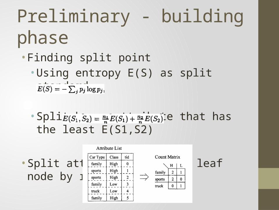
• Finding split point• Using entropy E(S) as split standard
• Split by an attribute that has the least E(S1,S2)
• Split attribute list into leaf node by record id
Preliminary - pruning phase
• Pruning phase • Compute the cost to determine if the subtree
should be prune or not• Lower the total cost will get better tree• MDL principle• the “best” tree is the one that can be encoded
using the fewest number of bits.

Preliminary - pruning phase
• Cost of Encoding Tree• the structure of the tree: 1 bit• internal node (1)• leaf (0)
• each split: lg(a) bits + value bits• the attribute• the value of attribute
• the classes of data records in each leaf of the tree

Preliminary - pruning phase
• Pruning algorithm• Leaf node: compute and return its own cost• Internal node: compare with the cost that
prune the sub-tree and not prune, choose smaller one• Stop when N is root

The PUBLIC Integrated Algorithm• Most algorithms for inducing decision trees• Building phase → Pruning phase
• Disadvantage in two phases of decision tree• PUBLIC (PrUning and BuiLding Integrated in
Classification)

The PUBLIC Integrated Algorithm• Similar to the build procedure

The PUBLIC Integrated Algorithm• Problem with applying the original pruning
procedure

The PUBLIC Integrated Algorithm• PUBLIC’s Pruning Algorithm• Under-estimation strategy• Three kinds of leaf nodes• Q ensures not expanded

Computation of Lower Bound on Subtree Cost• PUBLIC(1) : a cost at least 1• PUBLIC(S) : the cost of splits• PUBLIC(V) : cost of values• They are identical except for the value “lower
bound on subtree cost at N”.• They use increasingly accurate cost estimates for
“yet to be expanded” leaf nodes, and result in fewer nodes being expanded during the building phase.

Computation of Lower Bound on Subtree Cost• Estimating Split Costs• S: the set of records at node N• k: the number of classes for the records in S• ni be the number of records belonging to class
i in S, ni n≧ i+1 for 1 i < k ≦• a : the number of attributes• In case node N is not split, that is, s = 0, then
the minimum cost for a subtree at N is C(S)+1• For s > 0, the cost of any subtree with s splits
and rooted at node N is at feast:

Computation of Lower Bound on Subtree Cost• Algorithm for Computing Lower Bound on
Subtree Cost ─ PUBLIC(S)

Computation of Lower Bound on Subtree Cost• PUBLIC(S)• Calculates a lower bound for s = 0,…,k-1• For s = 0 : C(S)+1• For s > 0 :
• Takes the minimum of the bounds• Computes by iterative addition• O(klogk)

Computation of Lower Bound on Subtree Cost• Example: Let a “yet to be expanded” leaf node N
contain the following set S of data records.
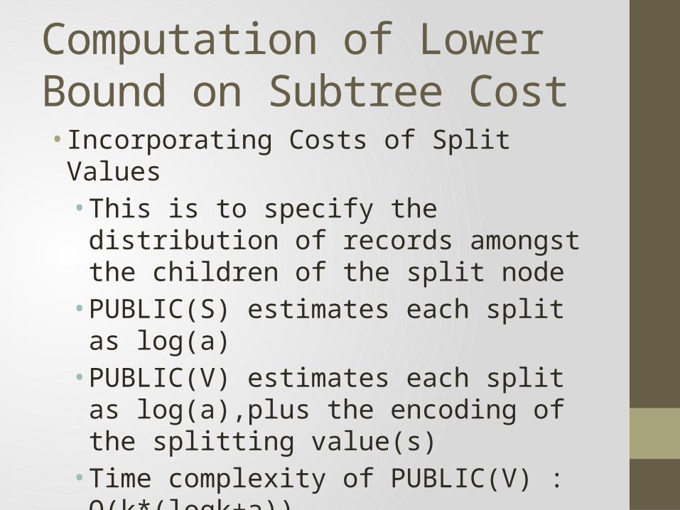
Computation of Lower Bound on Subtree Cost• Incorporating Costs of Split Values• This is to specify the distribution of records
amongst the children of the split node• PUBLIC(S) estimates each split as log(a)• PUBLIC(V) estimates each split as log(a),plus
the encoding of the splitting value(s)• Time complexity of PUBLIC(V) : O(k*(logk+a))

Experimental Results-Real-life Data Sets
Data Set breastcancer
car letter satimage shuttle vehicle yeast
No. of Categorical Attributes
0 6 0 0 0 0 0
No. of Numeric Attributes
9 0 16 36 9 18 8
No. of Classes 2 4 26 7 5 4 10
No. of Records(Train)
469 1161 13368 4435 43500 559 1001
No. of Records(Test)
214 567 6632 20000 14500 287 483
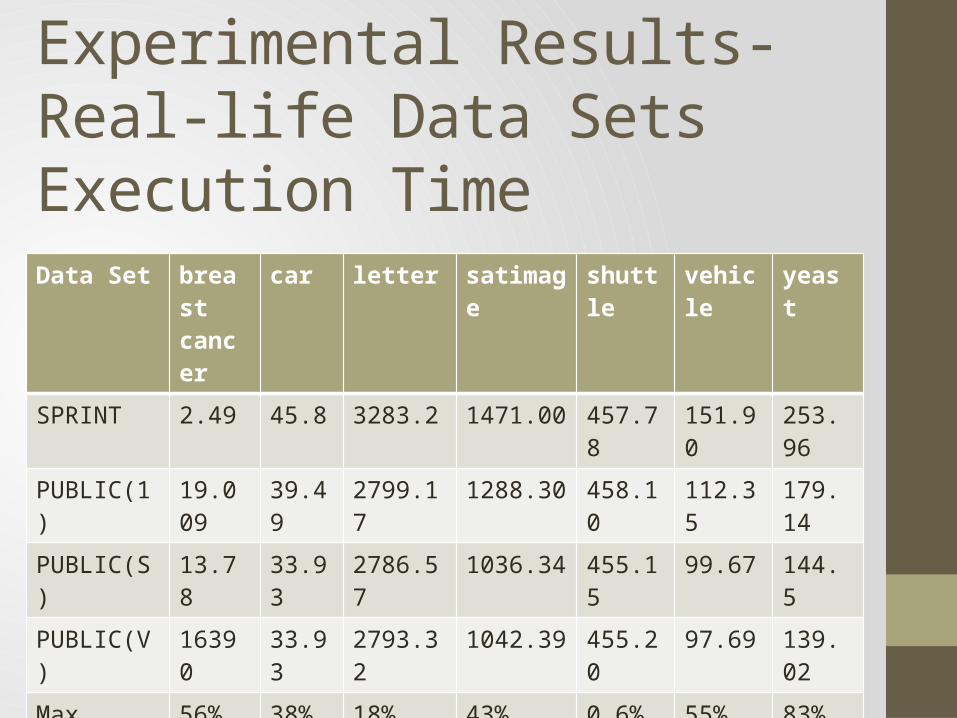
Experimental Results-Real-life Data Sets Execution Time
Data Set breastcancer
car letter satimage shuttle vehicle yeast
SPRINT 2.49 45.8 3283.2 1471.00 457.78 151.90 253.96
PUBLIC(1) 19.009 39.49 2799.17 1288.30 458.10 112.35 179.14
PUBLIC(S) 13.78 33.93 2786.57 1036.34 455.15 99.67 144.5
PUBLIC(V) 16390 33.93 2793.32 1042.39 455.20 97.69 139.02
Max Ratio 56% 38% 18% 43% 0.6% 55% 83%

Experimental Results-Synthetic Data Sets
Attribute Description Value
salary salary Uniformly distributed from 20000 to 150000
commission commission If salary >75000 then commission is zero else uniformly distributed from 10000 to 75000
age age uniformly distributed from 20 to 80
elevel education level uniformly chosen from 0 to 4
car make of the car uniformly chosen from 1 to 20
zipcode zip code of the town uniformly chosen from 9 to available zipcodes
hvalue value of the house uniformly distributed from 0.5k100000 to 1.5k00000 where k {0,.,9} depends on zipcode
hears years house owned uniformly distributed from 1 to 30
loan total loan amount uniformly distributed from 0 to 500000

Experimental Results-Synthetic Data Sets Execution Time
Predicate No.
1 2 3 4 5 6 7 8 9 10
SPRINT 1531 1471 1399 1413 1454 1471 1277 1978 1336 1627
PUBLIC(1)
714 720 654 707 769 760 615 875 676 783
PUBLIC(S)
607 604 553 617 656 653 559 741 589 689
PUBLIC(V)
574 593 520 575 615 587 510 708 567 666
Max Ratio
267% 359% 269% 246% 236% 251% 250% 279% 236% 244%

Experimental Results-Synthetic Data Sets Execution Time
Conclusion
• PUBLIC(l):simplest, building and pruning together
• PUBLIC(S):considers subtree with splits
• PUBLIC(V):computes the most accurate lower bound• • Experimental Results: real-life data & synthetic data • --> PUBLIC can result in significant performance.

Discussion
• In building phase, use GINI may have less space than compute entropy, but cost more time• Log needs log table, square cost time
• Add pruning phase back into PUBLIC to make the total node reduce• Reduce memory cost
31

Thank you!


