
Process Analysis Toolkit (PAT) 3.5 User
Manual
Table of contents
1. 1 Introduction
1.1 1.1 Preface
1.2 1.2 Organization
2. 2 Getting Started
2.1 2.1 Installation
2.2 2.2 Graphic User Interface
2.2.1 2.2.1 PAT Editor
2.2.2 2.2.2 PAT Simulator
2.2.3 2.2.3 Graph Difference Analysis
2.2.4 2.2.4 PAT Verifier
2.2.5 2.2.5 New Model Wizard
2.3 2.3 System Options
2.3.1 2.3.1 BDD Settings
2.4 2.4 LTL to Automata Converter
2.5 2.5 Using C# (C/C++/Java) Code as Libraries
2.5.1 2.5.1 External Static Methods
2.5.2 2.5.2 User Defined Data Type
2.5.3 2.5.3 Using Microsoft Contracts.htm
2.5.4 2.5.4 Using C/C++ Code in PAT
2.6 2.6 Keyboard Shortcuts
2.7 2.7 Command Line
3. 3 Process Analysis Toolkit
3.1 3.1 Communicating Sequential Programs (CSP#) module
3.1.1 3.1.1 Language Reference

3.1.1.1 3.1.1.1 Global Definitions
3.1.1.2 3.1.1.2 Process Definitions
3.1.1.3 3.1.1.3 Assertions
3.1.1.4 3.1.1.4 Expressions
3.1.1.5 3.1.1.5 Grammar Rules
3.1.1.6 3.1.1.6 Process Laws
3.1.1.7 3.1.1.7 Verification Options
3.1.2 3.1.2 CSP Module Tutorial
3.1.2.1 Bridge Crossing Example
3.1.2.2 Dining Philosophers Example
3.1.2.3 Multi-Lift System Example
3.1.3 3.1.3 Miscellaneous
3.2 3.2 Real-Time System (RTS) Module
3.2.1 3.2.1 Language Reference
3.2.1.1 3.2.1.1 Timed Process Definitions
3.2.1.2 3.2.1.2 Assertions
3.2.1.3 3.2.1.3 Grammar Rules
3.2.1.4 3.2.1.4 Verification Options
3.2.2 3.2.2 Real-Time System Tutorial
3.2.2.1 Fischer's Mutual Exclusion Example
3.2.2.2 Train Cross Control Example
3.3 3.3 Probability CSP (PCSP) Module
3.3.1 3.3.1 Language Reference
3.3.1.1 3.3.1.1 Probability Processes
3.3.1.2 3.3.1.2 Assertions
3.3.1.3 3.3.1.3 Grammar Rules
3.3.1.4 3.3.1.4 Verification Options
3.3.2 3.3.2 PCSP Module Tutorial
3.3.2.1 PZ86 Mutual Exclusion
3.3.2.2 Monty Hall Example

3.4 3.4 Probability RTS (PRTS) Module
3.4.1 3.4.1 Language Reference
3.4.1.1 3.4.1.1 PRTS Processes
3.4.1.2 3.4.1.2 Assertions
3.4.1.3 3.4.1.3 Grammar Rules
3.4.2 3.4.2 PRTS Module Tutorial
3.4.2.1 Multi-lifts System Example
3.5 3.5 Labeled Transition System (LTS) Module
3.5.1 3.5.1 Language Reference
3.5.1.1 3.5.1.1 Global Definitions
3.5.1.2 3.5.1.2 Primitive Process Definitions
3.5.1.2.1 Drawing
3.5.1.2.1.1 Navigation Tree
3.5.1.2.1.2 Canvas
3.5.1.2.2 State
3.5.1.2.3 Transition
3.5.1.3 3.5.1.3 Process Definitions
3.5.1.4 3.5.1.4 Verification Options
3.5.2 3.5.2 LTS Module Tutorial
3.5.2.1 3.5.2.1 Bridge Crossing Example
3.6 3.6 Timed Automata (TA) Module
3.6.1 3.6.1 Language Reference
3.6.1.1 3.6.1.1 Declarations
3.6.1.2 3.6.1.2 Process Definitions
3.6.1.2.1 Drawing
3.6.1.2.1.1 Navigation Tree
3.6.1.2.1.2 Canvas
3.6.1.2.2 State
3.6.1.2.3 Transition
3.6.1.3 3.6.1.3 Grammar Rules

3.6.2 3.6.2 TA Module Tutorial
3.6.2.1 3.6.2.1 Fischer's Protocol
3.6.2.2 3.6.2.2 Railway Control System
3.6.2.3 3.6.2.3 CSMA/CD Protocol
3.7 3.7 NesC Module
3.7.1 3.7.1 Language Reference
3.7.1.1 3.7.1.1 Drawing a Sensor Network
3.7.1.2 3.7.1.2 The NesC Language
3.7.1.3 3.7.1.3 TinyOS Library
3.7.1.4 3.7.1.4 Semantic Model
3.7.1.5 3.7.1.5 Assertions
3.7.2 3.7.2 nesC Module Tutorial
3.7.2.1 3.7.2.1 Individual Sensor Tutorial
3.7.2.1.1 BlinkApp Example
3.7.2.2 3.7.2.2 Sensor Network Tutorial
3.7.2.2.1 LeaderElection Protocol
3.8 3.8 Orc Module
3.8.1 3.8.1 Language Reference.htm
3.8.1.1 3.8.1.1 The ORC Language.htm
3.8.1.2 3.8.1.2 Addon for Verification.htm
3.8.1.3 3.8.1.3 Assertions.htm
3.8.1.4 3.8.1.4 Supported Sites.htm
3.8.1.5 3.8.1.5 Grammar Rules.htm
3.8.2 3.8.2 ORC Module Tutorial.htm
3.8.2.1 3.8.2.1 Metronome.htm
3.8.2.2 3.8.2.2 Concurrent Quicksort.htm
3.8.2.3 3.8.2.3 Auction Management.htm
3.9 3.9 Stateflow (MDL) Module
3.9.1 3.9.1 Language Reference
3.9.2 3.9.2 Stateflow Tutorial

3.9.2.1 3.9.2.1 Alarm Monitor
3.9.2.2 3.9.2.2 Stopwatch
3.9.2.3 3.9.2.3 Gear Shift
3.9.2.4 3.9.2.4 Fault-tolerant Fuel Controller
3.9.2.5 3.9.2.5 SB Logic
3.10 3.10 Security Module
3.10.1 3.10.1 Language Reference
3.10.1.1 3.10.1.1 Specification section
3.10.1.2 3.10.1.2 Verification section
3.10.1.3 3.10.1.3 Grammar Rules
3.10.2 3.10.2 SeVe Module Tutorial
3.10.2.1 3.10.2.1 Needham Schroeder Protocol
3.11 3.11 Web Service (WS) Module (obsolete)
3.11.1 3.11.1 Language Reference
3.11.1.1 3.11.1.1 Global Definitions
3.11.1.2 3.11.1.2 Web Service Choreography
3.11.1.3 3.11.1.3 Web Service Orchestration
3.11.1.4 3.11.1.4 Assertions
3.11.1.5 3.11.1.5 Grammar Rules
3.11.2 3.11.2 Web Service Tutorial
3.11.2.1 Online Shopping Example
3.12 3.12 UML into PAT
3.12.1 ATM Example
4. 4 Special Features
4.1 4.1 Fairness
4.2 4.2 Parallel Verification
4.3 4.3 Verification of Infinite Systems
4.4 4.4 Verification of Linearizability
4.5 4.5 Timed Zenoness Checking
5. 5 Developer Guild

5.1 5.1 PAT Architecture
5.2 5.2 PAT Class Diagram
5.2.1 5.2.1 GUI and Common Package
5.2.2 5.2.2 Module Package
5.3 5.3 PAT Extensions
5.3.1 5.3.1 Language Translation
5.3.2 5.3.2 Language Extension
5.3.3 5.3.3 Algorithm Extension
5.3.4 5.3.4 Module Extension
5.3.5 5.3.5 Using PAT as Library
5.4 5.4 Module Generator
5.4.1 5.4.1 Module Generation
5.4.2 5.4.2 Working with Generated Code
5.4.3 5.4.3 Example
6. 6 FAQs
6.1 Installation FAQ
6.2 Using PAT FAQ
7. 7 References
1. 1 Introduction
Welcome to Process Analysis Toolkit (PAT)!
PAT is a self-contained framework for to support composing, simulating and
reasoning of concurrent, real-time systems and other possible domains. It comes with
user friendly interfaces, featured model editor and animated simulator. Most importantly,
PAT implements various model checking techniques catering for different properties
such as deadlock-freeness, divergence-freeness, reachability, LTL properties with
fairness assumptions, refinement checking and probabilistic model checking. To
achieve good performance, advanced optimization techniques are implemented in PAT,

e.g. partial order reduction, symmetry reduction, process counter abstraction, parallel
model checking.
The main functionalities of PAT are listed as follows:
User friendly editing environment (multi-document, multi-language, I18N GUI and
advanced syntax editing features) for introducing models
User friendly simulator for interactively and visually simulating system behaviors;
by random simulation, user-guided step-by-step simulation, complete state graph
generation, trace playback, counterexample visualization, etc.
Easy verification for deadlock-freeness analysis, reachability analysis,
state/event linear temporal logic checking (with or without fairness) and
refinement checking.
A wide range of built-in examples ranging from benchmark systems to newly
developed algorithms/protocols.
We design PAT as an extensible and modularized framework, which allows user to
build customized model checkers easily. We provide a library of model checking
algorithms as well as the support for customizing language syntax, semantics, model
checking algorithms and reduction techniques, graphic user interfaces, and domain
specific abstraction techniques. Delightfully, PAT has been growing up to eleven
modules today to deal with problems in different domains including Real Time Systems,
Web Service Models, Probability Models, and Sensor Networks etc. In order to be state-
of-the-art, we are actively developing PAT to cope with latest formal-automated system
analysis techniques.
We have been using PAT to model and verify a variety of systems. Ranging from
recently proposed distributed algorithms, security protocols to real-world systems
like multi-lift and pacemaker systems. Previously unknown bugs have been discovered.
The experiment results (available in PAT web site) show that PAT is capable of verifying
systems with large number of states and outperforms the popular model checkers in
some cases. We have successfully demonstrated PAT as an analyzer for process

algebras in the 30th International Conference on Software Engineering (ICSE 2008)
[LiuSD08], the 21st International Conference on Computer Aided Verification (CAV
2009) [SunLDP09] and FSE 2010 [LIUSD10].
This manual will introduce you various aspects of PAT, including using PAT and
specific knowledge of different modules in PAT. In this chapter, we will discuss about
why we need system verification and what PAT is designed for. See Section 1.1
Preface. Also we will give an outline to show how this manual is organized and what are
the main topics covered. See Section1.2 Organization.
About PAT:
PAT project is initialized in School of Computing, National University of Singapore in
July 2007.
The key members designing PAT are:
Dr. SUN, Jun, Assistant Professor, Singapore University of Technology and
Design.
Dr. LIU, Yang, Senior Research Scientist, Temasek Laboratories and School of
Computing, National University of Singapore.
Dr. DONG, Jin Song, Associated Professor, School of Computing, National
University of Singapore.
Contact us:
Should you meet any difficulty using PAT or find bugs of PAT or have some
suggestion on improving PAT, please do not hesitate to contact any one of us.
Alternatively, you can send an email to [email protected].
Acknowledgement

We own thanks to research collaborators, including Prof. Jun Pang, Prof. Hai Wang,
Prof. Jing Sun, Prof. Wei Chen, Prof. Annie Y. Liu and Prof. Geguang Pu.
We would like to thank Prof. Jing Sun, Prof. Hugh Anderson, Prof. Jonathan S.
Ostroff for using PAT for the course teaching. Their valuable feedback made PAT more
suitable for teaching.
We are very grateful for the valuable comments and suggestions from professor
Tony Hoare, professor Joxan Jaffar, professor Jim Woodcock, professor Jim Davis,
professor Jens Palsberg, professor Auguston Mikhail, professor Kokichi FUTATSUGI,
professor Phil Brooke, professor Kenji Taguchi, professor Doron A. Peled so on.
We have special thanks to our Japanese user group, especially Hiroshi Fujimoto,
Kenji Taguchi, Masaru Nagaku, Toshiyuki Fujikura.
[TOP]
1.1 1.1 Preface
Why we need Process Analysis Toolkit?
To be able to verify the correctness of computer systems, no matter whether they
are hardware, software or a combination, is of great importance. Well, there are
essential problems which cannot be discovered by current techniques. For instance, the
concurrent bugs are among the most difficult to be found by testing, since they tend to
be non-reproducible or not covered by test cases [HUTH&Ryan04]. Thus it is well worth
having handy verification tools to simulate the system behaviors and verify critical
properties such as safety, concurrency, liveness and fairness. Then comes our Process
Analysis Toolkit ( PAT) !
What is PAT?

Process Analysis Toolkit ( also known as PAT, available at
http://www.patroot.com) is designed to apply state-of-the-art model checking
techniques for system analysis.
At first we developed this tool to investigate system ( specified using the classic
process algebra Communicating Sequential Processes - CSP) verification under
fairness assumptions. The motivation is that fairness assumptions are often necessary
in system verification practice in order to prove desirable system properties, whereas
existing languages and tools have limited support for fairness modeling as well as
verification. Since then, PAT has been evolved to be a self-contained framework to
support reach-ability analysis, deadlock-freeness analysis, full LTL ( linear temporal
logic) model checking, refinement checking as well as a powerful simulator. It is a
user-friendly model checker for all users.
Starting from PAT 2.0, we applied a modularized design to support the analysis of
the different system/languages. Each language is encapsulated as one module with
predefined APIs, which identify the ( specialized) language syntax, well-formed rules
as well as ( operational) formal semantics, and loaded at run time according to the
input model. This layered architecture allows new languages to be developed easily by
providing the syntax rules and semantics. Till now, eleven modules have been
developed, namely Communicating Sequential Processes ( CSP) module, Web
Service ( WS) module, Real-Time System Module, Probability CSP Module, Orc
Module, Security Module and NesC Module etc.. In the future, our targeted systems
include C# program and UML ( state chart and sequence diagrams) and so on.
Please refer to Chapter 3 the Process Analysis Toolkit for detailed information.
From PAT 3.0, we emphysis the extension and creating custimized model checkers,
which provides the different interfaces for domain experts to create their model
checkers with minimum efforts. There are several ways to create your dedicated model
checker which will be introduced in section 5.3 PAT extensions. You can create a new
module either by easy translation or extending the languange syntax or apply new

properties and corresponding checking algorithms or building a completely new module
following the steps and using pre-defined API as we will show you.
[TOP]
1.2 1.2 Organization
This manual is organized as follows:
Chapter 1 Introduction
Brief introduction about why we need system verification and what is Process
Analysis Toolkit and information related to PAT issues. And also give an outline
about how this manual is organized.
o 1.1 Preface
o 1.2 Organization
Chapter 2 Getting started
This chapter will give you the detailed and helpful information about how to
install, configure and use PAT.
o 2.1 Installation
o 2.2 Graphic User Interface
o 2.3 System Configuration
o 2.4 LTL to Automata Converter
o 2.5 Using C# Library
o 2.6 Keyboard Shortcuts
o 2.7 Command Line
o
Chapter 3 Process Analysis Toolkit
This chapter helps you with the detailed information about how to play with PAT,
including the depth knowledge about PAT's architecture and different modules.
Each module has a specific language reference and a tutorial part which shows

how PAT can be used in different domains such as reasoning about strict Real
Time System problems.
o 3.1 Communication Sequence Process Module
o 3.2 Real Time System Module
o 3.3 Probability CSP Module
o 3.4 Probability RTS Module
o 3.5 Labeled Transition System (LTS) Module
o 3.6 Timed Automata (TA) Module
o 3.7 NesC Module
o 3.8 Orc Module
o 3.9 Stateflow (MDL) Module
o 3.10 Secutiry Module
o 3.11 Web Service Module
o 3.12 Import UML into PAT
o
Chapter 4 Special Features
o 4.1 Fairness
o 4.2 Parallel Verification
o 4.3 Verification of Infinite Systems
o 4.4 Verification of Linearizability
o 4.5 Timed Zenoness Checking
o
Chapter 5 Developer Guide
o 5.1 PAT Architecture
o 5.2 PAT Class Diagram
o 5.3 PAT Extensions
o 5.4 PAT APIs
o 5.5 Module Generator
Chapter 6 FAQ
Questions and answers about installing and using PAT.

o Installation FAQ
o Using PAT FAQ
o
Chapter 7 References
Give a list of publications and books this manual referenced.
[TOP]
2. 2 Getting Started
This chapter will explain you how to install and configure PAT, as well as how the
friendly user interface helps you to start using PAT. Also a few advanced topics like
using C# code as library will also be discussed here. See the corresponding section for
detailed information.
Topics covered in this chapter are as follows:
System installation and configuration
Graphic User Interface including Editor, Simulator, Graph Difference Analysis,
Verifier and New Model Wizard
LTL to Automata Converter
Using C# (C/C++/Java) code as library
Keyboard Shortcuts
Using Command Line
When the first time you launch PAT, you will see this picture straightforward guiding
you to start with PAT!

[TOP]
2.1 2.1 Installation
2.1 Installation:
Install PAT 3.x in Windows XP, Vista and Windows Server 2000/2003, Windows 7:

1. You should have .NET Framework 4.0 above, which can be downloaded here.
2. Find PAT web site: go to http://www.patroot.com/ or alternatively search for
"Process Analysis Toolkit" in Google.
3. Download PAT: Click Download from the panel on the left and then follow the link
at the first line in the middle panel.
4. Register your information: Fill out the registration form and you will be re-directed
to the downloading page.
5. Install PAT: Double click the downloaded executable file and follow the
instruction.
6. Q&A: If you have problems on installing PAT, check out the FAQ.
Install PAT 3.x in Linux, Unix, Mac OS or more, please follow these steps:
1. You should install mono tool in your system which is freely available. Please
download from here according to your OS. Note that libmono-winforms2.0-cil
(plus its dependencies) may need be added in order to run PAT under Linux
(Ubuntu).
2. Download PAT 3.x from our website as (Step 2- 4) above. But choose the directly
executable version to some place in your computer.
3. In your computer, start terminal application, using the command cd to the
directory where you put "PAT 3.exe";
4. Type the command mono "PAT 3.exe" into terminal.(You might need to add
execute permission as chmod +x "./PAT 3.exe") Bingo! You will see the GUI of
our PAT.
5. Currently the latest mono 2.8.x has some problem on Mac, if you meet some
error related to winforms, please use the mono-2.6.7 which is available here.
Note: PAT runs faster in Windows than other OS. The reason is that mono is not as
fast as native .NET framework.
2.2 System requirements:

1. .NET framework 4.0 and Windows XP, Vista and Windows Server 2000/2003,
Windows 7. or
2. Mono tool for all other operating systems.
2.3 Update and Un-installation:
1. Automatic update when system is launched. (you can disable the auto update in
system configurations).
2. Easy un-installation from program list.
Note: Auto updating is not avaiable for 64 bit version of PAT. We suggest you to
download the latest version of 64 bit PAT from the website and install again.
[TOP]
2.2 2.2 Graphic User Interface
PAT comes with complete and user friendly graphic interface to make the tool handy
to use.
The graphic user interface consists of the following parts to allow users to edit the
model, simulate it and verify the properties of the model respectively. In this section, we

explain the GUI of the CSP module as the demonstrating example. The GUIs for other
modules are similar.
2.2.1 PAT Editor
2.2.2 PAT Simulator
2.2.3 Graph Difference Analysis
2.2.4 PAT Verifier
2.2.5 New Model Wizard
The system options are explained here.

[TOP]
2.2.1 2.2.1 PAT Editor

From PAT 3.0 onwards, PAT Editor provides a more preferable and intelligent way
of editing your model. The programmers' most favourable features are listed below.
Meanwhile, PAT editor also provides key action buttons and the full set of document
editing functions with a multi-document and I18N (multi-language) environment.
Keyword highlighting
IntelliSense
Model Explorer (F4)
Go to Declaration Function (F12)
Find Usage
Rename (F2)

A. The Keyword highlighting, as shown in the above figure, the keyword highlighting
are explained as follows:
the reserved keywords will be highlighted in blue.

the processes names will be bold and highlighted in dark blue automatically.
Symbols reserved for processes definition are shown in red.
LTL formulars in assertions will be bold and shown in red.
Comments are in green etc.
B. For the newly supported intelliSense, it can serve as an intelligent reminder for
keywords when you are inputting your model:
After you input an English letter for example 'a', it will automatically give out a list
containing all keywords starting with 'a' and the explanation of the corresponding
keyword. This is to better assist you in programming the model, and remind you
the useful hints.
After parsing the model, you will see the processes are also included in the list!
See the figure above the process Specification() is in the list after checking
grammar.
C. The Go to Declaration (F12) function is implemented for all variables, processes,
constants, declarations and channels in all modules.
To use this function, follow the steps:
Select a word in the editor and press F12, editor will bring you to the
definition of the word if there is one.
D. The Model Explorer (F4) function is recently supported for all modules. Press
F4 to open the explorer window and click refresh button, all the constants, variables,
processes etc. will be shown in the list. Parsing the model (by pressing F5) will also
refresh the model explorer. To access a particular item, you only have to double click it.
This function is extremely useful when the mode becomes quite big!
E. Find Usage: This function is to help user to quickly locate all the usage of the
selected text. It is useful especially in the large models with lots of variables, processes
etc. To use this function, right click the selected text and choose the Find Usage label in

the menu. For now, PAT is able to find usage for declarations, processes, variables,
channels and constants in a model.
F. Rename (F2): Using renaming function when you want to sysmetically and
safely change the name of a variable, it will automatically replace all the corresponding
usage of the variable with the new name. To use this function, select a word (process
name, variable, channel, constants and declaration) and press F2 (or right mouse click
on the selected word and choose rename label in the menu). A popup window will show
to ask for the new name. After you confirm, the changes will automatically apply to the
whole model.
After input the model, the four key actions you can perform by click the
corresponding buttons in the specification toolbar:
Check Grammar : check whether the model has correct grammar. If the grammar
is not accepted, there will be a pop-up of certain error message.
Simulation : simulate the model using simulator. The grammar needs to be
parsed first before the simulator to be shown.
Verification : verify the assertions using verifier. The grammar needs to be
parsed first before the verifier to be shown.
Graph Difference: generate the graph grouping the similar states and transitions
between two graphs. The grammar needs to be parsed first before the graph
difference analysis to be shown.
PAT provides different user interface languages: Chinese (Simplified), Chinese
(Traditional), English, Japanese, German and Vietnamese. You can switch between the
languages under toolbar View->Languages. System will remember your choice next
time it starts. Other languages will be added if there is a request.
The set of document editing functions are listed as follows:

New: create a new model and open it in the Editor. New model wizard is also
available now!
Open: open an existing model.
Save: save the model.
Save As : save the model as another file.
Email Model: email the current model to PAT team or friends.
Print: print the model.
LaTex Print: generate the LaTex text for the input model.
Recent files: view your records of edited files recently.
Exit: exit PAT by clicking it.
The set of text editing functions is listed as follows:
Cut, Copy, Paste, Select All
Find, Find Next, Replace
Zoom in and Zoom out or 100% Text size
Redo, Undo
Goto Line
Comment Selected Code: Make a block of codes as a comment for reference.
Uncomment Selected Code : Uncomment block of codes.
Outlining: Toggle the selected codes or toggle all the outlining for a clear view of
your model. You can expand them by click the '+' symbol by the side of line
number.
Bookmark: Add bookmarks to your code to memorise your ideas. You can view
the previous or next bookmark as well as deleting all the bookmarks through the
editing functions.
The set of featured editing functions is listed as follows:
Line Number Display
Highlight Current Line
Go to Previous Tab

Go to Next Tab
Close Current Tab
Drag and Drop a model into PAT to open it quickly
[TOP]
2.2.2 2.2.2 PAT Simulator
PAT's simulator allows users to interactively and visually simulate system behaviors.
The simulator is made up of four parts: Toolbar on the top, Interaction Pane, Data Pane
(showing the value of the variables at selected state) and Simulation Graph.
Select the process you want to simulate, the simulation tasks that can be performed
are described as follows.
Click the Simulate button to do a random simulation of the system. The simulator
will randomly select one enabled event at current state to execute. The
simulation will stop when there is no more enabled events are available or the
number of the visited states is bigger than the limit. Current state is shown in red
color in the graph.
Double click the event in the "Enabled Events" list to perform the step-by-step
simulation. The "Enabled Events" list will only show the enabled events for the
current state (shown in red color in the graph). Events shown in blue color are
unvisited events while black color are visited events for the current state.
Generate Graph button will generate the complete state graph in one click. The
number of states to be displayed is bounded by display limit (300 by default) to
avoid the non-termination of the model.
Select any state in the "Event Trace" list, then click the Play Trace button to play
the trace automatically starting from the selected state. You may go back to any
previous states.

Simulate Trace button allows users to write a script to perform automatic
simulation. After clicking it, a textbox is shown where you can writre the event
trace like phil.0.0, phil.0.1, eat.0 or a, b(5), tick. Each event is seprated by
comma and b(5) means you can perform b 5 times.
Click Reset button to reset the simulator to the initial state of the selected
process.
Note: the number of states that can be generated is limited to 300 by default. You
can change this number in the system configurations.
Counterexample visualization: Click the Simulate button in the Verifier to view the
counterexample. If the counterexample belongs to a LTL assertion, you can also view
the strongly connected component which generates the counterexample.
Easter egg : if you try the dining philosophers or sliding game example (in CSP
Module) in PAT, you would see a picture of the board in the simulator. We are
developing more pictures for other examples.
Tips of using Simulator:
You can move your mouse over the state and transition in the graph to see the
detailed information.
You can drag the node and edges in the Simulation Graph.
You can adjust the simulation speed in the toolbar settings button: very fast, fast,
normal, slow, very slow.
You can adjust the tooltip popup delay in the toolbar settings button: 5s, 10s,
20s, 40s, 60s.
You can hide all the tau transitions in the toolbar settings button.

[TOP]
2.2.3 2.2.3 Graph Difference Analysis
PAT also provides an interesting interface to generate difference graph from two
graphs generated in the Simulator. This function is developed to provide means for
comparing the differences between similar processes. For instance, you can use this

tool to generate a difference graph with your system and the abstracted model of your
system, or with the implementation and specification of your system.
The Graph Difference Analysis tool has several choices for different purposes of
users. Configure the tool before starting using:
From the tool bar:
Match Type: Complete or Partial match.
Match Result Display: Integrated or Separate (See the figures in the last row).
Graph Match Settings: Match State Structure, Match Process Parameters, Match
Event Details, Match if/guard Condition Expression; these four can be multiple choices;
Generate Difference Graph: press this button to generate the difference graph for
previously chosen graphs.
Match Result List: this button provides a list of matching results including matched
edges/nodes and unmatched edges/nodes in the left graph and the right graph.
Take the classic problem Dining Philosopher as an example, we generate the
difference graph from the system graph and the implementation graph.
First, generate the desired processes in Simulator separately and then choose the
corresponding graphs to be compared, such as the figure below:

Secondly, generate the difference graph in the Integrated(left) manner and the
Separate(right) manner respectively.


[TOP]
2.2.4 2.2.4 PAT Verifier
PAT Verifier allows users to check the assertions listed in the model. The verification
result will be shown in different hightling colors such as red for the assertion which is not
valid and green for the assertion which is valid. We provide two modes for verification,
e.g. The click mode and the batch mode. Both of the two modes support the following
options:
OPTIONS:

Admissible behaviors: This is essentially faireness type settings. PAT will
automatically enable the suitable fairness options (not supported in Orc Module) for the
user according to the model and the property selected. Notice that all fairness options
are disabled except for LTL assertions. For more information, please refer to section 4.1
Fairness and [SUNLDP09].
No Fairness: By default, this option is selected. In this setting, no fairness
assumption is applied to the system (even for event-annotated fairness).
Process Level Weak Fairness: Selecting this option means that for every process
in the system, if it is eventually always enabled, it must eventually always occur.
This option is similar to the one in SPIN. This option is only enabled, if the
system to be checked is an interleave or parallel composition.
Process Level Strong Local Fairness: Selecting this option means that for every
process in the system, if it is always eventually enabled, it must eventually
always occur. This option is only enabled, if the system to be checked is an
interleave or parallel composition.
Strong Global Fairness: Selecting this option means to apply strong global
fairness to the system, i.e., each transition must eventually always occur if it is
always eventually enabled.
Verification Engine: For all safety properties (e.g. deadlockfree, reachability,
refinement relation), in explicit model checking, PAT performs Depth-First-Search to
explore the state space for the purpose of fast verification. However, if there is any
counterexample, it is desired to have the shortest trace to find the bug quickly. Hence,
we provide this option to user such that PAT performs Breadth-First-Search to find the
shortest witness trace. Similarly symbolic model checking provides 3 search engines.
These search engines are both breadth first search with different directions.
Symbolic Model Checking using BDD with Forward Search Strategy: check the
safety property starting from the initial state, and go forward to check whether
bad states can be reachable from the inital state.

Symbolic Model Checking using BDD with Backward Search Strategy: check the
safety property starting from the bad states and go backward to check whether
the initial state is reachable.
Symbolic Model Checking using BDD with Forward-Backward Search Strategy:
check the safefy property starting from both initial state and bad states. At each
step, it will go forward from the initial state direction and go backward from the
bad state direction.
Some other choices are provided for specific properties such as Strongly
Connected Component Based Search (explicit model checking) and Symbolic Model
Checking using BDD for liveness properties. Please refer to Assertion page in the each
module's subsection of Language Reference in Section 3.
Time Out: This option allows you to limit the running time. If it is set to 0, then
system can run as long as it got a result or out of memory. If it is set to a
number greater than 0 then system will stop in due time if it hasn't got any result.
Generate Witness Trace: This option is provided to get the model checking result
without the counter example if exists.
MODES:
Click Mode: Use this mode to verify the properties, you have to manually click the
assertions one by one and choose the additional options described above.
Note: Multiple assertion selection is supported from the version 3.4.

Batch Mode: Use this mode, you can get all the properties of a batch of model
files verified with certain choices of options in one time. The whole verification result will
be written into an output file you defined. These results can also be converted to excel
files by clicking the button "Generate Excel Report".

To use this function, you can click the Tools tab in PAT's Editor, and select
Verification (Batch Mode).
[TOP]
2.2.5 2.2.5 New Model Wizard

To help the users to quickly start composing models, PAT provides a New Model
Wizard as listed as follows. Users can quickly generate model templates based on the
selection of modeling language and templates.
[TOP]
2.3 2.3 System Options
The option manual in PAT has the following settings:
General:
1. Auto-check for updates when PAT starts.
2. Auto save models when starting to do the simulation, verification and so on. This
will help user to keep the latest model in case of system failure. Uncheck it in
case you find this option is annoying.

3. Default Modeling Language is used to decide the modeling language when the
user clicking the New Button in the toolbar. The default modeling language is set
to be CSP Model here.
4. Specific model like CSP(RTS) Module, Web Service Model can also be
configured. See the right-handside figure
Simulation:
1. The maximum number of states to be displayed in the simulator. Default value is
300. More than 300 nodes in the simulator is hard to read usually.
Verification:
1. The initial size of the hash table used for the verification. Default value is 220. If
your model is small, then do not change it. But if your model is large to be like
more than million of states, change this value to a bigger one would be better.

[TOP]
2.3.1 2.3.1 BDD Settings
The BDD Settings is provided for user to set the special variable ranges. The BDD
performance is better if the provided variable ranges are more tight.
This tab includes 3 kinds of variables
The first two settings Variable Lower Bound/ Variable Upper Bound are used to
set the default variable range when the variable range is not provided in the
program.
For example:
var a:{0..2} = 0;

var b = 0;
According to the declaration, variable a's values are between 0 and 2 while b is not
provided the variable range, it will receive the default variable range in the BDD Setting
option tab which is {0..32}
The next three settings are used to set for the channel message. Maximum
Channel Message Length is the maximum of the channel message length where
channel message length is the number of parameters in a Channel Out
message, i.e., c!0.1.2 has the channel message length 3. Message Lower
Bound/ Message Upper Bound is the minimum/maximum values for parameters
in the Channel Out message.
Event Parameter Lower Bounds/ Event Parameter Upper Bounds are provided to
define the maximum number of parameter in an event name and the
minimum/maximum values of each parameter. According the current setting, the
maximum number of event parameters is 2 and each paramter is in the range
{0..10}. Therefore event names like event1.a, event2.i.j, and event3.0 are
acceptable. Using event name having more than 2 parameters like event4.a.b.c
or out of range paramters like event5.11 causes wrong result.

[TOP]
2.4 2.4 LTL to Automata Converter
PAT provides a useful tool to convert LTL formulae to Büchi Automata/Rabin
Automata/Streett Automata under toolbar Tools.

[TOP]
2.5 2.5 Using C# (C/C++/Java) Code as Libraries
Sometimes, it is difficult and inefficient to write some functions (e.g., Maths
calculation methods) or advanced data structures (e.g. Array, Stack, Queue and so on)
using PAT's syntax. To make this easier, PAT allows user to define static functions and
user defined data type in C# (C/C++/Java)language and use them in the models. These
C# classes are built as DLL and loaded when models import them. Once they are
defined, you can use them directly in any models.

Note: the method names are case sensitive.
PAT provides the management interface for C# libraries. Click Tool->C# Library
Editor and Compiler button in the toolbar menu, the following window will pop-up. You
can define your own functions. After input the functions, you can build the code and use
it immediately. You can write C# codes and compile them easily in this window.
The functions of the buttons are explained as follows:
New Library: load the template for creating static library.
New Data Type: load the template for creating user defined data type.
Open C# Code: load an existing C# code into the editor.
Save: save the text in the editor into C# code.
Release/Debug/Contracts: the compilation choice for the code. Debug option is
desired when using the System.Diagnostics.Debug.Assert method in C#.
Contracts are desired when using Microsoft Code Contracts in the C#.
Build DLL: build the code in the editor into a DLL, the default location of the DLL
will be the Lib folder under installation folder. Error messages will be shown if
there is any error during the compilation.
Close: close the editor.

PAT also provides another way to open the imported library. You can select the
imported library path and then right click the button, choose "open import/include file"
function to open it. This funcation can recognize absolute path, relative path to the
current model file and inside lib folder of pat installation.

[TOP]
2.5.1 2.5.1 External Static Methods
Some complicated calculations (e.g., algorithms, data operations and
computations) are difficult to implement in PAT's modeling language. It is easier to write
them using programming language like C#. We provide user such option to implement
the calculations using C# static methods and invoke these methods in PAT.

The following is one simple example of showing how to write static methods in C#.
using System.Collections.Generic;
using PAT.Common.Classes.Expressions.ExpressionClass;
// the namespace must be PAT.Lib, the class and method names can be arbitrary
namespace PAT.Lib {
public class PatList {
public static int[] ListAdd(int[] list, int element) {
List<int> newList = new List<int>(list);
newList.Add(element);
return newList.ToArray();
}
public static bool ListContains(int[] list, int element) {
foreach (int i in list) {
if (i == element) {
return true;
}
}
return false;
}
}
}
Note the following requirements when you create your own libraries:
The namespace must be "PAT.Lib", otherwise it will not be recognized. There is
no restriction for class names and method names.
Importing the PAT Expression name space using "using
PAT.Common.Classes.Expressions.ExpressionClass;".

All methods should be declared as public static. You can also use (private) static
variables and functions to support your methods.
The parameters must be of type "bool", "int", "int[]" (int array) or object (object
type allows user to pass user defined data type as parameter).
The number of parameters can be 0 or many.
The return type must be of type "void", "bool", "int", "short", "byte", "int[]" (int
array) or user defined data type.
The method names are case-sensitive.
Put the compiled DLLs in "Lib" folder of the PAT installation directory to make the
linking easy by using #import "DLL_Name"; or you can put the DLLs under same
folder as the model. If the DLLs are put in other places, you need to put the full
path of the DLLs after import keyword.
To import math library, please use #import "PAT.Math";
If your methods need to handle exceptional cases, you can throw PAT runtime
exceptions as illustrated as the following example.
public static int StackPeek(int[] array) {
if (array.Length > 0)
return array[array.Length - 1];
//throw PAT Runtime exception
throw new PAT.Common.Classes.Expressions.ExpressionClass.RuntimeException("Access an empty stack!");
}
To import the libraries in your model, users can using following syntax:
#import "PAT.Lib.Set"; //to import a library under Lib folder of PAT installation
path
#import "C:\Program Files\Intel\Set.dll"; //to import a library using absolute path
< syntax: following use please models, your in methods C# invoke the>

x = call(Max, 10, 2);
if(call(dominate, 3, 2))...
y = call(ArrayMax, [1,3,5]);
Note: the method names are case sensitive.
The build-in C# math functions you can use are listed as follows:
int Abs(int d)
int BigMul(int a, int b)
int Exp(int d)
int Max(int val1, int val2)
int Min(int val1, int val2)
int Pow(int val1, int val2)
int Sqrt(int d)
int Round(int a)
[TOP]
2.5.2 2.5.2 User Defined Data Type
PAT only supports integer, Boolean and integer arrays for the purpose of efficient
verification. However, advanced data structures (e.g., Stack, Queue, Hashtable and so
on) are necessary for some models. To support arbitrary data structures, PAT provides
an interface to create user defined data type by inheriting an abstract classes
ExpressionValue.
The following is one simple example showing how to create a hashtable in C#.
using System.Collections;
using PAT.Common.Classes.Expressions.ExpressionClass;
//the namespace must be PAT.Lib, the class and method names can be arbitrary

namespace PAT.Lib {
public class HashTable : ExpressionValue {
public Hashtable table;
/// Default constructor without any parameter must be implemented
public HashTable() {
table = new Hashtable();
}
public HashTable(Hashtable newTable) {
table = newTable;
}
public void Add(int key, int value) {
if(!table.ContainsKey(key)) {
table.Add(key, value);
}
}
public bool ContainsKey(int key) {
return table.ContainsKey(key);
}
public int GetValue(int key) {
return (int)table[key];
}
/// Return the string representation of the hash table.
/// This method must be overriden
public override string ToString() {
string returnString = "";
foreach (DictionaryEntry entry in table) {

returnString += entry.Key + "=" + entry.Value + ",";
}
return returnString;
}
/// Return a deep clone of the hash table
/// NOTE: this must be a deep clone, shallow clone may lead to strange behaviors.
/// This method must be overriden
public override ExpressionValue GetClone() {
return new HashTable(new Hashtable(table));
}
/// Return the compact string representation of the hash table.
/// This method must be overriden
/// Smart implementation of this method can reduce the state space and speedup
verification
public override string ExpressionID {
get {
string returnString = "";
foreach (DictionaryEntry entry in table) {
returnString += entry.Key + "=" + entry.Value + ",";
}
return returnString;
}
}
}
}

Note the following requirements when you create your own data structure objects:
The namespace must be "PAT.Lib", otherwise it will not be recognized. There is
no restriction for class names and method names.
Importing the PAT Expression name space using "using
PAT.Common.Classes.Expressions.ExpressionClass;".
Only public methods can be used in PAT models.
The parameters must be of type "bool", "int", "int[]" (int array) or object (object
type allow user to pass user defined data type as parameter).
Object type parameter are passed by reference, i.e., if the method changes the
parameter values, the effect will stay in the PAT model.
The number of parameters can be 0 or many.
The return type must be of type "void", "bool", "int", "short", "byte", "int[]" (int
array) or user defined data type.
The method names are case sensitive.
Put the compiled DLLs in "Lib" folder of the PAT installation directory to make the
linking easy by using #import "DLL_Name"; or you can put the DLLs under same
folder as the model. If the DLLs are put in other places, you need to put the full
path of the DLLs after import keyword.
If your methods need to handle exceptional cases, you can throw PAT runtime
exceptions as illustrated as the following example.
public static int StackPeek(int[] array) {
if (array.Length > 0)
return array[array.Length - 1];
//throw PAT Runtime exception
throw new PAT.Common.Classes.Expressions.ExpressionClass.RuntimeException("Access an empty stack!");
}
To import the libraries in your model, users can using following syntax:

#import "PAT.Lib.Hashtable"; //to import a library under Lib folder of PAT
installation path
#import "C:\Program Files\Intel\Hashtable.dll"; //to import a library using absolute
path
To declare the user defined types in your models, please use the following syntax:
var <HashTable> table; //use the class name here as the type of the variable.
var <HashTable> table = new HashTable(4); //initialize the variable using the
constructors provided.
To invoke the public methods in your models, please use the following syntax:
table.Add(10, 2); //public method invocation
if(table.ContainsKey(10))... //public method invocation with return values
table$column //public field or property reading and writting
Note that there is no difference between user defined types and normal variables
(e.g. var x =1;). Only when the process parameter is used as user defined types, it is
user's responsibility to make sure that the correct variable type is passed in since most
of PAT modules don't have explicit types. See the example below.
#import "PAT.Lib.Set";
var<Set> set1;
Q() = P(set1);
P(i) = initialize{i.Add(1);}-> ([i.GetSize() > 0] Skip);
Warning:
When the user defined data variable (declared as global variable) is used in
conditions (if-then-else/guard/while-loop), the operation should be side-effect free. One
example is the guard expression "i.GetSize() > 0" Otherwise the verification results may
not be correct.

When user defined data structure is used as process parameter, if the parameter in
the process updates the data structure, the verification/simulation maybe wrong and
unexpected. For instance the following example, i is an object used in both branch of
the choice operator, so the effect of executing add1 will stay even the actual branch
selected is add2. In the simulator, you will find that after executing event add2, the
value of set1 can become [1,2]. The root of this cause is the pointer problem. PAT will
give warnings for such usage during parsing. It is user's responsibility to make sure the
usage is correct.
#import "PAT.Lib.Set";
var<Set> set1;
Q() = P(set1);
P(i) = add1{i.Add(1);} -> Skip [] add2{i.Add(2);} -> Skip;
[TOP]
2.5.3 2.5.3 Using Microsoft Contracts.htm
PAT integrates the runtime checking of Microsoft Code Contracts in the external C#
codes. To use Contracts in your classes, you only need to choose the "contract" when
you build the DLL. In your code, contracts methods can be simply used as the normal
way: pre-condition, post-condition, invariant and assertions.
We are experimenting this feature. Please see DBM testing example in PAT for
more information.
[TOP]
2.5.4 2.5.4 Using C/C++ Code in PAT
Some complicated calculations (e.g., algorithms, data operations and
computations) are difficult to implement in PAT's modeling language. Beside supporting
calling C# methods, we also allow users to call C/C++ functions in PAT.

Suppose you have a C/C++ library, all you need is to create a C# interface using
that library and then call C# interface as External Static Method.Requirements to the C#
external static methods are also applied to the C/C++ functions.
Example:
You have a C function in the Plus.dll which return the sum of 2 integer numbers
extern "C" __declspec( dllexport ) plus(int a, int b);
For more information about how to export a C function, you may want to refer to
Exporting from a DLL Using __declspec(dllexport). The basic idea is adding "extern "C"
__declspec( dllexport )" before the interface declaration to mark it as be exported to the DLL.
You want to call this function in PAT. Firstly, you need to create an C# interface provoking this function. You may want to try as below:
public class CMethodDemo {
[DllImport(@"Lib\Plus.dll")]
public static extern int plus(int a, int b);
}
To call a DLL from C#, we need to declare a method as having an implementation from that DLL with the static and extern C# keywords. Then you need to attach the DllImport attribute to the method. For deeper understanding, following the tutorial Platform Invoke Tutorial from MSDN.
Then you build this as CMethodDemo.dll, put it and Plus.dll under "Lib" folder of the PAT installation directory. Last you can follow the External Static Methods to use this C# interface. Below is the PAT model using this feature. You can try this example in PAT, under CSP -> "Demonstrating Example" -> "C Library Demonstrating Example".
#import "PAT.Lib.CMethodDemo";
var x;
System = event{x = call(plus, 1,2);} -> out.x -> Skip;
#assert System() deadlockfree;

[TOP]
2.6 2.6 Keyboard Shortcuts
The set of document editing functions are listed as follows:
New (Ctrl+N)
Open (Ctrl+O)
Save (Ctrl+S)
Print (Ctrl+P)
The set of text editing functions is listed as follows:
Redo (Ctrl+Y)
Undo (Ctrl+Z)
Cut (Ctrl+X)
Copy (Ctrl+C)
Paste (Ctrl+V)
Select All (Ctrl+A)
Find (Ctrl+F)
Find Next (F3)
Replace (Ctrl+H)
Goto Line (Ctrl+G)
Comment Selection (Crtl + Shift + C)
Uncomment Selection (Crtl + Shift + U)
Toggle Outlining (Crtl + T)
Toggle All Outlinings (Crtl + Shift + T)
Toggle Bookmark (Crtl + B)
The set of featured editing functions is listed as follows:
Go to Previous Tab (Ctrl+Shift+Tab)
Go to Next Tab (Ctrl+Tab)

Close Current Tab (Ctrl+W)
After input the model, the three key actions you can perform by click the
corresponding buttons:
Help (F1)
Rename (F2)
Model Explorer (F4)
Check Grammar (F5)
Simulation (F6)
Verification (F7)
Graph Difference Analysis (F8)
Output Window (F9)
Goto Declaration (F12)
[TOP]
2.7 2.7 Command Line
PAT also supports running verification from the Console which is always favored by
programmers. And running from batch files using Console is extremely useful when you
have to run a batch of examples which spares you from starting at the monitor and
clicking the mouse all the way.
The main usage of command line is of the following format:
PAT.Console.exe [module] [options]* inputFile outputFile
for example: PAT.Console.exe -csp -sp DiningPhilosopher.csp result.txt .
For [module] part, the paragraph below lists all the supported commands
corresponding to different modules:

-csp: Verification using CSP Module. If there is no module option is given, this is
the default one.
-rts: Verification using Real-Time System Module.
-pcsp: Verification using Probabilistic CSP Module.
-prts: Verification using Probabilistic Real-Time System Module.
-module short name: Put the short name of your module, which should be the
folder name of your module.
For [options] part, here is the list for all the choices:
-b: (B)atch mode, the inputFile will be the batch file containing lines of examples.
Each line shall have the following format: -f inputFile
-d: (D)irectory mode, the inputFile shall be the input directory name. All examples
inside the directory will be executed.
Please use only -b or -d
-behavior n: specify the admissible behavior as integer value n. Default value is
0.
-engine n: specify the search engine as integer value n. Default value is 0.
-help: print HELP information.
-nc: (N)o (C)ounterexample display.
-on: (O)n-the-fly Normalization. Suggest not to use, since static normalization is
usually faster.
-v: (V)erbose mode.
-ver: (VER)sion.
The UML related of command line usage is of the following two formats:
PAT.Console.exe -uml inputFile outputFile
The command firstly translates inputFile into a CSP# model and outputs the CSP#
model to outputFile.

PAT.Console.exe -uml inputFile1 inputFile2 outputFile
The command firstly translates inputFile1 and inputFile2 into two CSP# models
respectively, say input1 and input2, then verifies whether input1 refines input2 in the
trace semantics, i.e. the assertion "#assert input1 refines input2", and outputs the result
to outputFile.
[TOP]
3. 3 Process Analysis Toolkit
Critical system requirements like safety, liveness and fairness play important roles in
software/system specification, development and testing. It is desirable to have handy
tools to simulate the system behaviors and verify critical properties. Process Analysis
Toolkit (also known as PAT) is design to apply state-of-the-art model checking
techniques for system analysis. It supports reachability analysis, deadlock-freeness
analysis, full LTL (linear temporal logic) model checking, refinement checking as well as
a powerful simulator. It is a user-friendly model checker for Windows users.
Starting from PAT 2.0, we applied a layered design to support the analysis of the
different system/languages. The figure below shows the architecture design of PAT. For
each supported system (e.g., distributed system, service oriented computing, bio-
system, security protocols, sensor network and real-time system), a dedicated module
is created in PAT, which identifies the (specialized) language syntax, well-formness
rules as well as (operational) formal semantics. The formally defined operational
semantics of the target language translates the behaviors of a model into a Labeled
Transition System (LTS). During this translation, domain specific abstraction can be
applied to the input model, e.g., data abstraction, zone abstraction and environment
abstraction. LTS serves as the internal representations of the input models, which can
be automatically explored by the verification algorithms or used for simulation. If there is
any counterexample is identified, then it can be animated in the simulator. The

advantage of this design allows the developed model checking algorithms to be shared
by all modules.
This architecture allows new languages to be developed easily by providing the
syntax rules and semantics. Till now, eleven modules have been developed, namely
Communicating Sequential Processes (CSP) Module, Real-Time System Module,
Probability CSP Module, Probability RTS Module, Labeled Transition System Module,
Timed Automata Module, NesC Module, ORC Module, Stateflow(MDL) Module,
Security Module and Web Service (WS) Module. In the future, our targeted systems
include distributed systems, UML (state chart and sequence diagrams) and so on.
The main functionalities of PAT are listed as follows:

User friendly editing environment (multi-document, multi-language, I18N GUI and
advanced syntax editing features) for introducing models
User friendly simulator for interactively and visually simulating system behaviors;
by random simulation, user-guided step-by-step simulation, complete state graph
generation, trace playback, counterexample visualization, etc.
Easy verification for deadlock-freeness analysis, reachability analysis,
state/event linear temporal logic checking (with or without fairness) and
refinement checking.
A wide range of built-in examples ranging from benchmark systems to newly
developed algorithms/protocols.
PAT has been applied to a variety of different systems to prove properties or
identifying bugs. Indeed, previously unknown bugs have been found using PAT. We
have successfully demonstrated PAT as an analyzer for process algebras in the 30th
International Conference on Software Engineering (ICSE 2008) [LiuSD08] and the 21st
International Conference on Computer Aided Verification (CAV 2009) [SunLDP09]. In
summary, PAT is a self-contained framework for automated analysis on concurrent and
real-time systems.
[TOP]
3.1 3.1 Communicating Sequential Programs (CSP#) module
PAT's CSP# module supports a rich modeling language named CSP#(pronounced
'CSP sharp', short for Communicating Sequential Programs) which combines high-level
modeling operators like (conditional or non-deterministic) choices, interrupt,
(alphabetized) parallel composition, interleaving, hiding, asynchronous message
passing channel, etc., with programmer-favored low-level constructs like variables,
arrays, if-then-else, while, etc.. It offers great flexibility on how to model your systems.
For instance, communication among processes can be either based on shared memory
(using global variables) or message passing (using asynchronous message passing or
CSP-style multi-party barrier synchronization). The high-level operators are based

on the classic process algebra Communicating Sequential Processes (CSP). Our
design principle for CSP# is to maximally keep the original CSP as a sub-language of
CSP#, whilst offering a connection to the data states and executable data operations.
The above illustrates the work flow of the CSP Module. System analysis in PAT is
supported in two ways, namely, simulation or model checking. The visualized simulator
allows the users to interactively play with their models, by choosing one of the enabled
actions at a time, let the computer to generate system traces randomly or even build the
complete state graph (given it is not very large). The model checkers embedded in PAT
are designed to apply state-of-the-art model checking techniques for systematic
analysis. Users can state assertions in various forms, and by just clicking one button,
PAT would tell whether the assertion is true or not (in which case a counterexample is
generated and ready to be simulated). PAT has a number of different model checking
algorithms for efficient verification of different properties. For instance, an efficient
depth-first-algorithm is used to verify safety properties by identifying a bad state, an
SCC-based algorithm is used to verify liveness properties by identifying a bad loop and

an SCC-based algorithm to verify liveness properties under fairness by identifying a fair
bad loop (refer to our paper [SUNLDP09] for detail).
CSP module is distinguished in a number of aspects from existing model checkers.
In the following, we briefly introduce the two of them. To reveal the full details, please
refer to our publications.
The LTL model checking algorithm in PAT is designed to handle a variety of fairness
constraints efficiently. This is partly motivated by recently developed population
protocols, which only work under weak, strong local/global fairness. The other
motivation is that the current practice of verification is deficient under fairness. Two
different approaches for verification under fairness are supported in PAT, targeting
different users. For ordinary users, one of the following options may be chosen and
applied to the whole system: weak fairness or strong local/global fairness. The model
checking algorithm works by identifying the fair execution at a time and checks whether
the desirable property is satisfied. Notice that unfair executions are considered
unrealistic and therefore are not considered as counterexamples. Because of the
fairness, nested depth-first-search is not feasible and therefore the algorithm is based
on an improved version of Tarjan's algorithm for identifying strongly connected
components. We have successfully applied it to prove or disprove (with a
counterexample) a range of systems where fairness is essential. In general, however,
system level fairness may sometimes be overwhelming. The worst case complexity is
high and, much worse, partial order reduction is not feasible for model checking under
strong local/global fairness. A typical scenario for network protocols is that fairness
constraints are associated with only messaging but not local actions. We thus support
an alternative approach, which allows users annotate individual actions with fairness.
Notice that this option is only for advanced users who know exactly which part of the
system needs fairness constraints. Nevertheless this approach is much more flexible,
i.e., different parts of the system may have different fairness. Furthermore, it allows
partial order reduction over actions which are irrelevant to the fairness constraints,
which allows us to handle much larger systems.

LTL formulas assert properties over each and every single execution of the system,
PAT allows users to reason about behaviors of a system as a whole by refinement
checking. Refinement checking is to verify whether an implementation's behaviors
follow the specifications. PAT supports six notions of refinements based on different
semantics, namely trace refinement, stable failures refinement, failures divergence
refinement and each of the above refinement augmented with data refinement. A
refinement checking algorithm (inspired by the one implemented in FDR but extended
with partial order reduction) is used to perform refinement checking on-the-fly.
Refinement checking in FDR only compares the traces (e.g., event sequences) of the
implementation and the specification. For practical systems (other than those specified
with process algebra), it may be desirable to also compare the data structures. For
instance, linearizability is an important correctness criteria for concurrent data structure.
Informally, it requires that the data structure accessed by multiple processes
concurrently must be updated as if the processes access it sequentially. To establish a
refinement relationship, not only the event of accessing the data structure must be
compared between a sequential specification and a concurrent implementation, but also
the data structure itself must be checked. We thus provide a user option to state
whether to check for data refinement.
[TOP]
3.1.1 3.1.1 Language Reference
The input language of CSP Module CSP# is mainly influenced by the classic
Communicating Sequential Processes (CSP [Hoare85]). Nonetheless, we extend CSP
with various useful language features to reach our goal. Examples include shared
variables, arrays, asynchronous message passing channels and event annotations
which capture a variety of fairness constraints.
Our modeling language is designed for automated system analysis. There are two
other popular modeling languages working for the same purpose, namely machine

readable CSP (which we will refer to as CSPM) supported by the refinement checker
FDR [AWR97] and Promela which is supported by the model checker SPIN [GJH97].
Compared to CSPM, CSP# supports additional language features like shared
variables, asynchronous communication channels and event associated
programs, which offers users great flexibility in modeling. Furthermore, we give
an interpretation of state/event Linear Temporal Logic in CSP# semantics
framework, which allows temporal logic based model checking of CSP# models.
Compared to Promela, CSP# supports more process constructs, i.e., Promela is
based on a subset of CSP, whereas all CSP models are valid CSP# models. In
particular, CSP# inherits the classic trace, stable failures and failures/divergence
semantics from CSP, and therefore, allows us to perform a variety of refinement
checking. CSP# is also remotely related to other languages which are designed
for model checking.
The language constructs of CSP# may be categorized into the following groups.
The first group is the core subset of CSP operators, including event-prefixing,
internal/external choices, alphabetized lock-step synchronization, conditional
branching, interrupt, recursion, etc.
The second group includes those language constructs which can be regarded as
"syntactic sugar" (to CSP), including global shared variables, and asynchronous
channels. It has long been known that CSP is capable of modeling shared
variables or asynchronous channels as processes. However, the dedicated
language constructs offer great usability and may make the verification more
efficient.
The third group is a set of event annotations. It is known that process algebra like
CSP or CCS specifies safety only. The event annotations offer a flexible way of
modeling fairness using an event based compositional language.
The last group is the language for stating assertions, which later may be
automatically verified using the built-in verifiers.

The language syntax structures are listed as follows. The complete grammar rules
and process laws can be found in Section 3.1.1.5 and Section 3.1.1.6 respectively.
3.1.1.1 Global Definitions
Model Name
Global Constants
Global Variables/Arrays
Asynchronous Channels
Macro
3.1.1.2 Process Definitions
Stop
Skip
Event Prefixing
Statement Block inside Events
Channel Input/Output
Sequential Composition
External/Internal Choice
Conditional Choice
Case
Guarded Processes
Interleaving
Parallel Composition
Interrupt
Hiding
Atomic Sequence
Recursion
Assert
3.1.1.3 Assertions

Deadlock-freeness
Divergence-free
Reachability Analysis
Linear Temporal Logic (LTL)
Refinement/Equivalence
[TOP]
3.1.1.1 3.1.1.1 Global Definitions
Model Name
First of all, you can give a name for your model using the following syntax in the first
line of your model. The model name is used internally as an ID for simulator to find the
correct drawing pictures, if any. It is optional.
//@@Model Name@@
Constants
A global constant is defined using the following syntax,
#define max 5;
#define is a keyword used for multiple purposes. Here it defines a global constant
named max, which has the value 5. The semi-colon marks the end of the 'sentence'.
Note: the constant value can only be integer value (both positive and negative) and
Boolean value (true or false).
Constant enumeration can be defined using keyword enum. For example, enum
{red, blue, green}; is the syntactic sugar for the following:
#define red 0;

#define blue 1;
#define green 2;
Variables/arrays
A global variable is defined using the following syntax,
var knight = 0;
wherevar is a key word for defining a variable and knight is the variable name.
Initially, knight has the value 0. Semi-colon is used to mark the end of the 'sentence' as
above. We remark the input language of PAT is weakly typed and therefore no typing
information is required when declaring a variable. Cast between incompatible types may
result in a run-time exception.
A fixed-size array may be defined as follows,
var board = [3, 5, 6, 0, 2, 7, 8, 4, 1];
where board is the array name and its initial value is specified as the sequence, e.g.,
board[0] = 3. The following defines an array of size 3.
var leader[3];
All elements in the array are initialized to be 0.
Note for multi-dimensional array: PAT supports multi-dimensional arrays by
converting them into one dimensional arrays. You can declare and use multi-
dimensional arrays as follows (Note that here, the N should be a constant). The only
restriction is that you can not assign multi-dimensional array constant to multi-
dimensional arrays variables. To initialize a multi-dimensional array, you need to do it
explicitly in some events.
var matrix[3*N][10];

Note: To assign values to specific elements in an array, you can use event prefix.
For example:
P() = a { matrix[1][9] = 0 } -> Skip;
Variable range specification: users can provide the range of the variables/arrays
explicitly by giving lower bound or upper bound or both. In this way, the model checkers
and simulator can report the out-of-range violation of the variable values to help users to
monitor the variable values. The syntax of specifying range values are demonstrated as
follows.
var knight : {0..} = 0;
var board : {0..10} = [3, 5, 6, 0, 2, 7, 8, 4, 1];
var leader[N] : {..N-1}; //where N is a constant defined.
Array Initialization: To ease the modeling, PAT supports fast array initialization using
following syntax.
#define N 2;
var array = [1(2), 3..6, 7(N*2), 12..10];
//the above is same as the following
var array = [1, 1, 3, 4, 5, 6, 7, 7, 7, 7, 12, 11, 10];
In the above syntax, 1(2) and 7(N*2) allow user to quickly create an array with same
initial values. 3..6 and 12..10 allow user to write quick increasing and decreasing loop to
initialize the array.
User defined type: To ease the modeling, PAT allows users to define any data
structures and use them in PAT models. The following shows the syntax.
var<Type> x ; //default constructor of Type class will be called.
var<Type> x = new Type(1, 2); //constructor with two int parameters will be
called.

Hidden variable: To simplify the model, PAT introduces the hidden variables which
can be used as normal variables. The only difference is that hidden variable is a kind of
secondary variable, which is not included in the state details. The idea of secondary is
to use redundant variable to make the modeling easier.
var a; var b;
hvar difference; //secondary variable to store the difference between a and b.
Note: It is user's responsibility to make sure that hidden variables don't introduce any
new states. If you not sure about this, you can change hvar to var to see any difference
in terms of states in the simulation or verification.
Channels
In PAT, process may communicate through message passing on channels. A
channel is declared as follows,
channel c 5;
wherechannel is a key word for declaring channels only, c is the channel name and
5 is the channel buffer size; Channel buffer size must be greater or equal to 0. Notice
that a channel with buffer size 0 sends/receives messages synchronously. This is used
to model pair-wise synchronization, which involves two parties. Barrier-synchronization,
which involves multiple parties, is supported by following CSP's approach, i.e.,
alphabetized parallel composition.
Note: Currently, channel array is also supported.
channel c[4] 5;
Macro
In addition, the key word #define may be used to define macro. For instance,

#define goal x == 0;
where goal is the name of the macro and x == 0 is what goal means. A macro name
is used in the same way as global constant is used. For instance, given the above
definition, we may write the following,
if (goal) { P } else { Q };
which means if the value of x is 0 then do P else do Q. We remark that macro can
be used in LTL formulae.
Furthermore, macro can take in parameters as defined below. When calling the
macro, the keyword call is used. The macro expression can be any possible expression
in PAT (if, local variable declarition, while, assignment).
#define multi(i,j) i*j;
System = if (call(multi, 3,4) >12 ) { a -> Skip } else { b -> Skip };
Note that following usage of macro definitions are allowed in PAT, which means that
macro definitions can be a fragment of code to be used in the model.
var x = 0;
var y = 0;
var z = 0;
#define reset1 {x = 0; y = 0};
#define reset(i) {x = i; y = i};
P = e1{z = 0; reset1} -> Skip;
Q = e2{z = 2; call(reset, 1)} -> Skip;
Model Inclusion
If the model is too big, you can split the model to several files and include them in
the main model by using the include keyword. For example,

#include "c:\example.csp";
If the model is in the same folder of the main model, you can only put the file name.
Note that: Nested inclusion in files are also possible in PAT, and duplicated inclusion
will be ignored.
To open the included file, you can select the file path, then right click the button and
choose "open import/include file" function to open it. This funcation can recognize both
absolute path and relative path to the current model file. The picture below shows how
to open an included file.

[TOP]
3.1.1.2 3.1.1.2 Process Definitions
A process is defined as an equation in the following syntax,
P(x1, x2, ..., xn) = Exp;
where P is the process name, x1, ..., xn is an optional list of process parameters and
Exp is a process expression. The process expression determines the computational
logic of the process. A process without parameters is written either as P() or P. A
defined process may be referenced by its name (with the valuations of the parameters).
Process referencing allows a flexible form of recursion.
Stop
The deadlock process is written as follows,
Stop
The process does absolutely nothing.
Skip
The process which terminates immediately is written as follows,
Skip
The process terminates and then behaves exactly the same as Stop.
Event prefixing
A simple event is a name for representing an observation. Given a process P, the
following describes a process which performs e first and then behaves as specified by
process P.

e -> P
where e is an event. An event is the abstraction of an observation. Event prefixing is
a common construct for describing systems. The following describes a simple vending
machine which takes in a coin and dispatches a coffee every time.
VM() = insertcoin -> coffee -> VM();
Where event insertcoin models the event of inserting a coin into the machine and
event coffee models the event of getting coffee out of the machine. An event may be in
a compound form, e.g., x.exp1.exp2 where x is a name and exp1 and exp2 are
expressions which are composed variables (e.g., process parameters, channel input
variables or global variables). For instance,
Phil(i) = get.i.(i + 1)%N -> Rest();
where i is a parameter of the process. We remark event expressions which contains
global variables, though allowed, may result in runtime exception if combined with
alphabetized parallel composition. Refer to parallel composition for details.
Note: event name is an arbitrary string of form ('a'..'z'|'A'..'Z'|'_')
('a'..'z'|'A'..'Z'|'0'..'9'|'_')*. However, global variable names, global constant
names, process names, process parameter names, propositions names can not be
used as event name. One exception is the channel names are allowed, because we
may want to use channel name in a specific process to simulate the channel behaviors
and use refinement checking to compare with real channel events.
Statement Block inside Events (aka Data Operations)
An event can be attached with assignments which update global variables as in the
following example,
add{x = x+1;} -> Stop;

where x is a global variable.
In general, an event may be attached with a statement block of a sequential program
(which may contain local variables, if-then-else, while, math function etc.). This kind of
event-prefix process is called data operation in PAT. The exact syntax of the statements
can be found in Grammar Rules. Notice that the sequential program is considered as an
atomic action. That is, no interleaving of other processes before the sequential program
finishes. In other words, once started, the sequential program continues to execute until
it finished without being interrupted. From another point of view, the event can be
viewed as a labeled piece of code. The event name is used for constructing meaningful
counterexamples (or associating fairness with the code, as discussed below). For
instance, the following process can be used to find the maximum value of a given array.
var array = [0,2,4,7,1,3];
var max = -1;
P() = findmax{
var index = 0;
while (index < 6) {
if (max < array[index]) {
max = array[index];
}
index = index+1;
};
} -> P();
Note: both global variable (e.g., array, max) and local variables (e.g., index) are
allowed to be used and updated in the sequential program. While process arguments
and channel input variables can only be used without being updated. The scope of the
local variable is only inside the sequential program and starts from the place of
declaration. PAT does not support process level local variables so that there is no need

to maintain a changing heap/stack to gain the efficiency. Alternatively, process level
local variables can be modeled using global variables easily.
Note: Data operation supports local variable array, assume the following process is
valid in PAT:
event {var array[5];} -> Process
where local variable array's(here is the array) elements are initialized to zero.
Note: the semi-colon in the last expression in the statement block is optional for the
simplicity of modeling.
Note: PAT supports two assignment syntax sugars ++, --. x++ is same as x=x+1. y-- is
same as y = y-1. y=x++ is same as x = x +1; y = x;. There is no support for
other shorthands, such as ++b , --b , b *= 2 , b += a , etc. Where needed, their effect
can be reproduced by using the non-shortened equivalents. The following example
shows the usage of ++ and --, where the final values of x and y are both 3.
var x = 2;
var y;
P() = add{x++;} -> minus{x--;} -> event{y=x++;} -> Skip;
Invisible Events
User can explicitly write invisible event (i.e., tau event) by using keyword tau,
e.g., tau -> Stop. In the tau event, statement block can still be attached. With the
support of tau event, you can avoid using hiding operator to explicitly hide some visible
events by name them tau events. The second way to write an invisible event is to skip
the event name of a statement block, e.g., {x=x+1;} -> Stop, which is equivalent to
tau{x=x+1;} -> Stop.
Channel output/input

Processes may communicate through channels. Channel input/output is written in a
similar way as simple event prefixing. Let P be a process expression.
c!a.b -> P -- channel output
c?x.y -> P -- channel input
c?1 -> P -- channel input with expected value
c?[x+y+9>10]x.y-> P -- channel input with guard expression
Where c is a channel, a and b are expressions which evaluates to values (at run
time), while x and y are (local) variables which take the input values. A channel must be
declared before it is used. For channel output, the compound value evaluated from both
a and b is stored in the channel buffer (FIFO queue) if the buffer is not full yet. If the
buffer is full, the process waits. For channel input c?x.y, the top element on the buffer is
retrieved and then assigned to local free variables x and y if the buffer is not empty.
Otherwise, it waits. For channel input c?1, the top element on the buffer is retrieved if
the buffer is not empty and the top element value is 1. Otherwise, it waits. For channel
input c?[x+y+9>10]x.y, the top element on the buffer is retrieved and then assigned to
local free variable x and y if the buffer is not empty, and the guard condition x+y+9>10 is
true. Otherwise, it waits. Note that in channel input, you can write expressions after c?,
but the expressions can not contain any global variables. You can put arbitrary number
of variables/expressions in the channel output/input by separating them using '.'. The
following example demonstrates how channel communication is used.
channel c 1;
Sender(i) = c!i -> Sender(i);
Receiver() = c?x -> a.x -> Receiver();
System() = Sender(5) ||| Receiver();

PAT supports synchronous channel communication, i.e., the channel output and
its matching channel input are engaged together. The synchronous channel event will
be displayed as c.exp for channel output c!exp and channel input c?x. To do
synchronous channel communication, simply set the size of the channel to be 0. All the
channel communications for non-zero channel are asynchronous.
Channel communication can also attach program for both synchronous and
asynchronous channel.
channel c 0; //or channel c 1;
var x = 1;
P = c!x{ x = 2 } -> P;
Q = c?y{ x = y; } -> Q;
A = P ||| Q;
For the example above, the execution sequence is c!x -> (x = 2) -> c?y -> (x = y).
Note: Channel input variables' scope is after the channel input event and
within residing process. They can be referenced in the scope, but not updated.
Note: Parameter variables can be used in the expressions of channel input, e.g., P(i)
= c?i.i+1 -> Skip. In this case, once the value of parameter i is known, i and i+1 will be
instantiated to constants, so that only matching channel output data will be
received. Furthermore, local free variable in channel input can also be used in follow-up
channel input's expressions. e.g., P() = c!5 -> c?x -> c!6 -> c?x+1 -> Skip; In this case, x
is 5 and P can execute to Skip. Global variables CAN NOT be used in channel input
expressions!
PAT also support channel arrays, which is a syntax suger to make the modeling
easier if the channels are parameterized. The following syntax demonstrates how to use
the channel array.

channel c[3] 1;
Sender(i) = c[i]!i -> Sender(i);
Receiver() = c[0]?x -> a.x -> Receiver() [] c[1]?x -> a.x -> Receiver() [] c[2]?x -> a.x -
> Receiver();
System() = (||| i:{0..2}@Sender(i) ) ||| Receiver();
Note: Two or N dimentional channel array can be simulated by using 1 dimentional
channel array. Hence, we don't provide syntax support for that. For example channel
c[3][5] 1 is same as channel c[15] 1, and c[2][3]!4 -> Skip is same as c[2*N+3]!4 -> Skip,
where N is the first dimention.
Channel operations
PAT provides 5 channel operations to query the buffer information of asynchronous
channels: cfull, cempty, ccount, csize, cpeek. The usage of these operations follows the
normal static method call, i.e., call(channel_operation, channel_name). The meaning of
each operation is explained below.
cfull: a boolean function to test whether the an asynchronous channel is full or
not. e.g. call(cfull, c).
cempty: a boolean function to test whether the an asynchronous channel is
empty or not. e.g. call(cempty, c).
ccount: an integer function to return the number of elements in the buffer of an
asynchronous channel. e.g. call(ccount, c).
csize: an integer function to return the buffer size of an asynchronous channel.
e.g. call(cfull, c).
cpeek: return the first element of an asynchronous channel. e.g. call(cpeek, c).

Note: Parsing error message will be poped up if these operations are applied to a
synchronous channel.
Note: Run time exception will be thrown if trying to cpeek an empty buffer.
Sequential composition
A sequential composition is written as,
P; Q
where P and Q are processes. In this process, P starts first and Q starts only when
P has finished.
General/External/Internal choice
In PAT (as in CSP), we distinguish among general choice, external choice and
internal choice. General choice is resolved by any event. A general choice is written as
follows,
P [] Q
The choice operator [] states that either P or Q may execute. If P performs an event
first, then P takes control. Otherwise, Q takes control. Notice that the semantic is a bit
different from the external choice below.
External choice is resolved by the environment, e.g., the observation of a visible
event (i.e., not tau event). Notice that if the first event of both P and Q is visible, then
P[]Q and P[*]Q are equivalent. An external choice is written as follows,
P [*] Q

The choice operator [*] states that either P or Q may execute. If P performs a visible
event first, then P takes control. If Q performs a visible event first, then Q takes control.
Otherwise, the choice remains.
Internal choice introduces non-determinism explicitly. The following models an
internal choice,
P <> Q
where either P or Q may execute. The choice is made internally and non-
deterministically. Non-determinism is largely undesirable at design or implementation
stage, whereas it is useful at modeling stage for hiding irrelevant information. For
instance, it can be used to model the behaviors of a black-box procedure, where the
exact details of the implementation are not available.
The generalized form of general/external/internal choice is written as,
[] x:{1..n}@ P(x) -- which is equivalent to P(1) [] ... [] P(n)
[*] x:{1..n}@ P(x) -- which is equivalent to P(1) [*] ... [*]
P(n)
<> x:{1..n}@ P(x) -- which is equivalent to P(1) <> ... <>
P(n)
Conditional Choice
A choice may depend on a Boolean expression which in turn depends on the
valuations of the variables. In PAT, we support the classic if-then-else as follows,
if (cond) { P } else { Q }
if (cond1) { P } else if (cond2) { Q } else { M }

where cond is a Boolean formula. If cond evaluates to true, the P executes,
otherwise Q executes. Notice that the else-part is optional. The process if(false) {P}
behaves exactly as process Skip.
PAT also provides atomic conditional choices, which perform the condition checking
and first operation of P/Q together. This allows users to simulate CAS operator in
distributed systems. The syntax is following:
ifa (cond) { P } else { Q }
PAT provides blocking conditional choices, which are similar to guarded process.
The only difference is that the checking of blocking condition and the execution of P are
separated in ifb. The syntax is following. Note that there is no else in ifb.
ifb (cond) { P }
Note: Side effect (i.e., update of the variable value) is not allowed in if condition
(similarly for guarded process and case process below). This restriction is mainly for
using C# code in if condition. For example, a Boolean method isEmpty of a user defined
list variable returns a false and also adds an element to the list. We add this restriction
is purely for performance reason. If you really want to achieve this effect, you can put
the method call in an event prefix, and store the returned value in a global
Boolean variable. The global variable can then be used in the if condition then.
Case
A generalized form of conditional choice is written as,
case {
cond1: P1
cond2: P2
default: P
}

where case is a key word and cond1, cond2 are Boolean expressions. if cond1 is
true, then P1 executes. Otherwise, if cond2 is true, then P2. And if cond1 and cond2 are
both false, then P executes by default. The condition is evaluated one by one until a
true one is found. In case no condition is true, the default process will be executed.
Guarded process
A guarded process only executes when its guard condition is satisfied. In PAT, a
guard process is written as follows,
[cond] P
where cond is a Boolean formula and P is a process. If cond is true, P executes.
Notice that different from conditional choice, if cond is false, the whole process will wait
until cond is true and then P executes.
Interleaving
Two processes which run concurrently without barrier synchronization written as,
P ||| Q
where ||| denotes interleaving. Both P and Q may perform their local actions without
synchronizing with each other except termination events. If one process generates
termination event, this termination event cannot executed directly unless all processes
are emitting a termination event. For example the following process will deadlock due to
this constraint.
Skip ||| Stop
Notice that P and Q can still communicate via shared variables or channels. The
generalized form of interleaving is written as,
||| x:{0..n} @ P(x)

PAT supports grouped interleaving processes or even infinite number of processes
running interleavingly, similarly, for parallel composition and internal/external
choices. All the syntaxes below are valid.
||| {50} @ P(); //50 P() running interleavingly.
|| {..} @ Q(); //infinite number of Q() running in parallel.
[] x:{0..2} @ ( (||| {x} @ P) ||| (||| {x} @ Q()); // this is equivalent
to (Skip|||Skip)[]((||| {1} @P()) ||| (||| {1} @Q()) ) [] ((||| {2} @P()) |||(||| {2} @Q()));
Note: ||| {0} @ P() is same as Skip.
Note: Looping variables can also be used in the process inside as process
parameter. For example, the following definitions are all valid in PAT.
||| x:{0..3} @ (a.x -> Skip)
|| x:{0..3} @ (a.x -> Skip \ {a.x})
[] x:{0..3} @ (ch!x -> Skip)
Note: in grouped processes, e.g., []x:{0..n}@P or ||| {0} @ P() , n can be a global
constant or process parameter, but not a global variable. We make this restriction for
the performance reason. For example, the following definitions are all valid in PAT.
#define n 10; |||x:{0..n}@P;
P(n) = |||x:{0..n}@Q;
Parallel composition
Parallel composition of two processes with barrier synchronization is written as,
P || Q

where || denotes parallel composition. Different from interleaving, P and Q may
perform lock-step synchronization, i.e., P and Q simultaneously perform an event. For
instance, if P is a -> c -> Stop and Q is c -> Stop, because c is both in the alphabet of P
and Q, it becomes a synchronization barrier. Therefore, at the beginning, only a can be
engaged. After that, c is engaged by P and Q at the exactly same time. In general, all
events which are in both P and Q's alphabets must be synchronized. Notice that, which
events are synchronization barriers depends on the alphabets of P and Q. In order to
know what are the enabled actions, we therefore must first calculate the alphabets.
In tools like FDR, the shared alphabet of a parallel composition must be explicitly
given. In PAT, however, we have a procedure to automatically calculate alphabets. The
alphabet of a process is the set of events that the process takes part in. For instance,
given the process defined as follows,
VM() = insertcoin -> coffee -> VM();
The alphabet of VM() is exactly the set of events which constitute the process
expression, i.e., {insertcoin, coffee}. However, calculating the alphabet of a process is
not always trivial. It may be complicated by two things. One is process referencing. The
other is process parameters. In the above example, the process reference VM()
happens to be the same as the process whose alphabet is being calculated. Thus, it is
not necessarily to unfold VM() again. Should a different process is referenced, we must
unfold that process and get its alphabet. For instance, assume VM() is now defined as
follows,
VM() = insertcoin -> Inserted();
Inserted() = coffee -> VM();
To calculate the alphabet of VM(), we must unfold process Inserted() and combine
alphabets of Inserted() with {insertcoin}. Notice that a simple procedure must be used to
prevent unfolding the same process again. However, even with such a procedure, it

may still be infeasible to calculate mechanically the alphabet of a process.
The complexity is due to process parameters. For instance, given the following process,
P(i) = a.i -> P(i+1);
Naturally, the unfolding is non-terminating. In general, there is no way to solve this
problem. Therefore, PAT offers two compromising ways to get the alphabets. One is to
use a reasonably simple procedure to calculate a default alphabet of a process. When
the default alphabet is not as expected, an advanced user is allowed to define the
alphabet of a process manually. We detail the former in the following.
First of all, alphabet of processes are calculated only when it is necessary, which
means, only when a parallel composition is evaluated. This saves a lot of computational
overhead. Processes in a large number of models only communicate through shared
variables. If no parallel composition is present, there is no need to evaluate alphabets.
We remark that when there is no shared abstract events, process P ||| Q and P || Q are
exactly the same. Therefore, we recommend ||| when appropriate. When a parallel
composition is evaluated for the first time, the default alphabet of each sub-process is
calculated (if not manually defined). The procedure for calculating the default alphabet
works by retrieving all event constituting the process expression and unfolding every
newly-met process reference. It throws an exception if a process reference is met twice
with different parameters (which probably indicates the unfolding is non-terminating). In
such a case, PAT expects the user to specify the alphabet of a process using the
following syntax,
#alphabet P {...};
where P is process name and {...} is the set of events which is considered its
alphabet. Notice that the event expressions may contain variables. The rules is that if
process P(X) is defined, you may have alphabet definitions as follows,
#alphabet P {a.X};

Once the alphabets of P and Q are identified, we calculate their intersection. If P is
ready to perform an event which is not in the intersection, it may simply proceed, so
does Q. If P is ready to perform an event in the intersection, it has to wait until Q is also
ready to perform this event and then proceed together.
Remarks: Data operations (i.e. the events attached with programs) are not counted
in the calculation of alphabets to avoid data race on updating same global variables.
The detailed explanation and examples are available here (Question 3).
Remarks: If process P is expected to have different alphabets in different places in
the specification, a dummy may be defined to associate different alphabet with the
same process.
Q1() = P();
#alphabet Q1 {x};
Q2() = P();
#alphabet Q2 {y};
The philosophy is that we see both the process expression and alphabet as
signatures of a process (i.e., processes with the same process expression but different
alphabets are essentially different processes!).
The generalized parallel composition is written as,
|| x:{0..n} @ P(x);
The alphabet of each P(x) is calculated. An event can be engaged if and only if all
processes whose alphabet contains this event are ready to perform it.
Remarks: The syntax sugar indexed event list can be used in the definition of
alphabets. For example:

#define N 2;
P = e.0.0 -> e.0.1 -> e.0.2 -> turns -> e.1.0 -> e.1.1 -> e.1.2 -> e.2.0 -> e.2.1 -
> e.2.2 -> P;
#alphabet P { x:{0..N}; y:{0..N} @ e.x.y };
The above definitions define the alphabet of process P as the set of all events
except event turns appearing in its proces definition.
Interrupt
Process P interrupt Q behaves as specified by P until the first visible event of Q is
engaged which could be at any execution point of process P, and then the control
transfers to Q. An execution trace of process P interrupt Q is just a trace of P up to an
arbitrary point when the interrupt occurs, followed by any trace of Q.
The following is an example,
Err() = exception -> Err();
Routine() = routine -> Routine();
ExceptionHandling() = Routine() interrupt exception ->
ExceptionHandling() ;
System = Err() || ExceptionHandling();
where Routine() is a process which performs normal daily task, Err() is a process
modeling errors happened in the environment and ExceptionHandling() is a process
which performs necessary actions for error handling. For System, whenever an
exception occurs (modeled as event exception), process ExceptionHandling() takes the
control over.
Note: For process P interrupt Q, the interrupting event from Q must be a visible
event (not tau). If a tau event is detected, a runtime exception will be thrown.
Hiding

Process P \ A where A is a set of events turns events in A to invisible ones. Hiding is
applied when only certain events are interested. Hiding may be used to introduce non-
determinism. The following is an example,
dashPhil() = Phil() \ {getfork.1, getfork.2, putfork.1, putfork.2};
Phil() = getfork.1 -> getfork.2 -> eat -> putfork.1 -> putfork.2 -> Phil();
where process Phil() specifies a philosopher who gets two forks in order and then
eats and then puts down both forks in the same order. Process dashPhil(), however,
hides the events of getting up or putting down the forks. We can imagine that the
philosopher is so quick that no one can tell how he gets the forks. People can only tell
when he is eating. By hiding those events, the rest of the system can not observe those
hidden events. We remark that hiding is often used to prevent unwanted
synchronization in parallel composition.
Note: The syntax sugar indexed event list can be used for defining a set of events
with the same prefix. For example, the definition for process dashPhil() can be rewritten
as the following.
dashPhil() = Phil() \ { x:{1..2} @ getfork.x, y:{1..2} @ putfork.y} ;
Atomic Process
The keyword atomic allows user to associate higher priority with a process, i.e., if the
process has an enabled event, the event will execute before any events from non-
atomic processes. The syntax is atomic{P}, where P is any process definition.
If a sequence of statements is enclosed in parentheses and prefixed with the
keyword atomic, this indicates that the sequence is to be executed as one super-step,
not to be interleaved by other processes. In the interleaving of process executions, no
other process can execute statements from the moment that an event in an atomic
process is enabled until the last enabled one has completed. The sequence can contain
arbitrary process statements, and may be non-deterministic. Once an atomic process is

enabled, it immeidately gains a higher priority. It continues to execute until it is
disabled. Once all atomic processes are enabled, other non-atomic processes are then
allowed to execute. If multiple atomic processes are enabled, then they interleave each
other. In the following example, process P and Q will interleave each other, whereas W
will excute only after event c and f have occurred.
channel ch 0;
P = atomic { a -> ch!0 -> b -> c -> Skip};
Q = atomic { d -> ch?0 -> e -> f -> Skip};
W = g -> Skip
Sys = P ||| Q ||| W;
Note: Since PAT 3.4.2, the semantics of atomic process changed a little bit. In the
example below, before PAT 3.4.2, event a and d are enabled at the same time when
process Sys starts. In PAT 3.4.2, only d is enabled because enabled atomic process
has higher priority than enabled events. This change allows us to use atomic
consistently in CSP module and RTS module.
P = a -> atomic { b -> c -> Skip};
Q = atomic { d -> e -> f -> Skip};
Sys = P ||| Q;
Note: atomic sequences can be used for state reduction for model checking,
especially if the process is composed with other processes in parallel. The number of
states may be reduced exponentially. In a way, by using atomic, we may partial order
reduction manually (without computational overhead). The general rule is that local
events which are invisible to the verifying property and independent to other events
shall be associated with higher priority.
Note: an atomic process inside other atomic process has no effect at all.
Recursion

Recursion is achieved through process referencing flexibly. The following process
contains mutual recursion.
P(i) = a.i -> Q(i);
Q(i) = b.i -> P(i);
System() = P(1) || Q(2);
Note: when invoking a process, the parameters can be any valid expression, e.g.
P(x), P(x+1), P(new List()). Only when the process parameter is used as user defined
types, it is user's responsibility to make sure that the correct variable type is passed in
since most of PAT modules don't have explicit types. See the example below.
#import "PAT.Lib.Set";
var<Set> set1;
Q() = P(set1);
P(i) = initialize{i.Add(1);}-> ([i.GetSize() > 0] Skip);
Warning: when user defined data structure is used as parameter, if the parameter in
the process updates the data structure, the verification/simulation maybe wrong and un-
expected. For instance the following example, i is an object used in both branch of the
choice operator, so the effect of executing add1 will stay even the actual branch
selected is add2. In the simulator, you will find that after executing event add2, the
value of set1 can become [1,2]. The root of this cause is the pointer problem.
#import "PAT.Lib.Set";
var<Set> set1;
Q() = P(set1);
P(i) = add1{i.Add(1);} -> Skip [] add2{i.Add(2);} -> Skip;
It is straightforward to use process reference to realize common iterative
procedures. For instance, the following process behaves exactly as while (cond) {P()};
Q() = if (cond) {P(); Q()};

Assert
Assertion process allows user to add an assertion in the program. PAT simulator
and verifiers will check the assertion at run time. If the assertion is failed, a PAT runtime
exception will be thrown to the user and the evaluation is stoped. The syntax of
Assertion is as follows,
var x = 1;
P = assert(x > 0); e{x = x-1;} -> P;
[TOP]
3.1.1.3 3.1.1.3 Assertions
An assertion is a query about the system behaviors. In PAT, we support a number of
different assertions (still increasing). We support the full set of Linear Temporal Logic
(LTL) as well as classic refinement/equivalence relationships.
Deadlock-freeness
Given P() as a process, the following assertion asks whether P() is deadlock-free or
not.
#assert P() deadlockfree;
Where both assert and deadlockfree are reserved keywords. PAT's model checker
performs Depth-First-Search or Breath-First-Search algorithm to repeatedly explore
unvisited states until a deadlock state (i.e., a state with no further move except for
successfully terminated state) is found or all states have been visited.
Divergence-free
Given P() as a process, the following assertion asks whether P() is divergence-free
or not.

#assert P() divergencefree;
Where both assert and divergencefree are reserved keywords. Given a process, it
may perform internal transitions forever without engaging any useful events, e.g., P = (a
-> P) \ {a};, In this case, P is said to be divergent. Divergent system is usually
undesirable.
Deterministic
Given P() as a process, the following assertion asks whether P() is deterministic or
not.
#assert P() deterministic;
Where both assert and deterministic are reserved keywords. Given a process, if it
is deterministic, then for any state, there is no two out-going transitions leading to
different states but with same events. E.g, the following process is not deterministic.
P = a -> Stop [] a -> Skip;
Nonterminating
Given P() as a process, the following assertion asks whether P() is nonterminating or
not.
#assert P() nonterminating;
Where both assert and nonterminating are reserved keywords. PAT's model checker
performs Depth-First-Search or Breath-First-Search algorithm to repeatedly explore
unvisited states until a terminating state (i.e., a state with no further move, including
successfully terminated state) is found or all states have been visited. The following
process is deadlockfree, but not nonterminating.
P = a -> Skip;

Reachability
Given P() as a process, the following assertion asks whether P() can reach a state at
which some given condition is satisfied.
#assert P() reaches cond;
Where both assert and reaches are reserved keywords and cond is a proposition
defined as a global definition. For instance, the following code segment asks whether
P() can reach a state at which x is negative.
var x = 0;
P() = add{x = x + 1;} -> P() [] minus{x = x -1;} -> P();
#define goal x < 0;
#assert P() reaches goal;
In order to tell whether the assertion is true or not, PAT's model checker performs a
depth-first-search algorithm to repeatedly explore unvisited states until a state at which
the condition is true is found or all states have been visited.
To further query about variable values, PAT allows user to find the minimum value or
maximum value of some expressions in all reachable traces. The following coin
changing example show how to minimize the number of coins during the reachability
search.
var x = 0;
var weight = 0;
P() = if(x <= 14)
{
coin1{x = x + 1; weight =weight + 1;} -> P() [] coin2{x = x + 2; weight
= weight + 1;} -> P() [] coin5{x = x + 5; weight = weight + 1;} -> P()
};
#define goal x == 14;

#assert P() reaches goal with min(weight);
Linear Temporal Logic (LTL)
In PAT, we support the full set of LTL syntax. Given a process P(), the following
assertion asks whether P() satisfies the LTL formula.
#assert P() |= F;
where F is an LTL formula whose syntax is defined as the following rules,
F = e | prop | [] F | <> F | X F | F1 U F2 | F1 R F2
where e is an event, prop is a pre-defined proposition, [] reads as "always" (also can
be written as 'G' in PAT), <> reads as "eventually" (also can be written as 'F' in PAT), X
reads as "next", U reads as "until" and R reads as "Release" (also can be written as 'V'
in PAT).
An LTL formula can be evaluated over an infinite sequence of truth evaluations and
a position on that path. The semantics for the modal operators is given as follows.

Informally, the assertion is true if and only if every execution of the system satisfies
the formula. Given an LTL formula, PAT's model checker firstly invokes a procedure to
generate a Buchi automaton which is equivalent to the negation of the formula. Then,
the Buchi automaton is composed of the internal model of P() so as to determine
whether the formula is true for all system executions or not. Refer to [SUNLDP09] for
details. For instance, the following assertion asks whether the philosopher can always
eventually eat or not (i.e., non-starvation).
#assert Phil() |= []<>eat;
Note: event e can be component event like eat.0. e can also be channel event like
"c!3.8" or "c?19". Double quotation marks are needed when writing channel events due
to the special characters ! and ?. Synchronous channel events can be written as c.3.8.

#assert Phil() |= []<> eat.0 && "c!3";
Note: In LTL, if there is synchronous channel, its input (?) or output (!) event will be
renamed to synchronous event (.) after parsing.
[](c1!2 -> <> c2?3) will be changed to [](c1.2 -> <> c2.3)
Note: when two or more X are used together, leave a space between them. XX will
be mis-recognized as a proposition.
Refinement/ Equivalence
In PAT, we support FDR's approach for checking whether an implementation
satisfies a specification or not. That is, by the notion of refinement or equivalence.
Different from LTL assertions, an assertion for refinement compares the whole
behaviors of a given process with another process, e.g., whether there is a subset
relationship. There are in total 3 different notions of refinement relationship, which can
be written in the following syntax.
#assert P() refines Q() -whether P() refines Q() in the trace semantics;
#assert P() refines<F> Q() -whether P() refines Q() in the stable failures
semantics;
#assert P() refines<FD> Q() -whether P() refines Q() in the failures
divergence semantics;
PAT's model checker invokes a reachability analysis procedure to repeatedly
explore the (synchronization) product of P() and Q() to search for a state at which the
refinement relationship does not hold.
[TOP]
3.1.1.4 3.1.1.4 Expressions

Expressions are used in models together with processes. This section explains the
supported expression types and their usage.
Expression Types
1. Boolean Logical Expression: Two boolean logic operators OR and AND are
supported in PAT using symbol '||' and '&&' respectivly. The conditional-AND/OR
operator performs a logical-AND/OR of its bool operands, but only evaluates its
second operand if necessary.
2. Relational Operators contains the equal and not equal relation asl well as other
relations. They are expressed using the following symbols in PAT particularly:
o Equal '=='
o Not Equal '!='
o Other Relational operators: '<', '>', '<=', '>='
3. Arithmatic Operators contains the additive and multiplicative expressions which is
represented in the model using '+'/ '-' and '*', '/', '%' (modulo operator).
4. Unary Operators contains '+', '-' for positive or negtive values, '!' for negation of
boolean expressions.
5. Increment '++' or Decrement operators '--' increase or decrease the variable by 1
respectively.
6. If Expresson: The conditions in If can be expressions and their conbinations we
have introduced above. Then it has the similar meaning and usage as common
programming languages. Note that this if expression can only contain
expressions in the than or else branches, but the if process in the model can only
contains processes in the than or else branches.
7. While Expression: Similar as if expressions, while expression takes expresions of
type 1-4 or their combinations as condition and behaves just like it has defined
in common programming languages.
Note: Expressions of type 1-5 can be composed to be complex expressions. And
this composed expression will be parsed in the priority of 5 to 1 (i.e. the precedence

order). For example, if a, b, c are defined as variables, the following complex expression
is a valid expression.
if ((a % 2 == 0) || ( ((a++) <= b) && (b == c)) )
Indexed Boolean Expression
The indexed expression is a syntax sugar for grouping a list of OR or AND
expressions together overal a range of variables. The syntax is following:
A typical example is as follows:
var x[3];
P = if(&& i:{0..2}@(x[i] == 0)){bingo -> Skip};
Expression Macro Definition
Users can define expression macro using define keywork and use the macro in the
model or assertiosn.
var x;
#define goal x < 0;
[TOP]
3.1.1.5 3.1.1.5 Grammar Rules
specification
: (specBody)*
;
specBody
: library

| letDefintion
| definition
| assertion
| alphabet
| define
| channel
;
library
: '#' 'import' STRING ';' //import the library by full dll path or DLL name under the
Lib folder
| '#' 'include' STRING ';' //include the other models by full path or file name if under
the same folder of current model
;
channel
: 'channel' ID ('[' additiveExpression ']')? additiveExpression ';'
;
assertion
: '#' 'assert' definitionRef
(
( '|=' ( '(' | ')' | '[]' | '<>' | ID | STRING | '!' | '?' | '&&' | '||' | 'xor'| '->' | '<->' |
'/\\' | '\\/' | '.' | INT )+ )
| 'deadlockfree'
| 'nonterminating'
| 'divergencefree'
| 'deterministic'
| 'reaches' ID withClause?
| 'refines' definitionRef
| 'refines' '<F>' definitionRef
| 'refines' '<FD>' definitionRef
)
';'
;
withClause
: 'with' ('min' | 'max') '(' expression ')'
;
definitionRef
: ID ('(' (argumentExpression(',' argumentExpression)*)? ')')?
;
alphabet

: '#' 'alphabet' ID '{' eventList(',' eventList )* '}' ';'
;
define
: '#' 'define' ID '-'? INT ';'
| '#' 'define' ID ('true' ';'
| 'false' ';')
| 'enum' '{' a=ID(',' b=ID)* '}' ';'
| '#' 'define' ID dparameter? dstatement ';'
;
dparameter
: '(' ID (',' ID )* ')'
;
dstatement
: block
| expression
;
block
: '{' (s=statement)* (e=expression)? '}' //At least a statement or expression has to be
specified, i.e. s and e cannot be both null.
;
statement
: block
| localVariableDeclaration
| ifExpression
| whileExpression
| expression ';'
| ';'
;
//local variable that can be used in the block
localVariableDeclaration
: 'var' ID ('=' expression)? ';'
| 'var' ID '=' recordExpression ';'
| 'var' ID ('[' expression ']')+ ('=' recordExpression)? ';'
;
expression
: conditionalOrExpression ('=' expression)?
;

conditionalOrExpression
: '||' indexedExpression
| conditionalAndExpression ( '||' conditionalAndExpression )*
;
conditionalAndExpression
: '&&' indexedExpression
| conditionalXorExpression ( '&&' conditionalXorExpression)*
;
conditionalXorExpression
: 'xor' indexedExpression
| bitwiseLogicExpression ( 'xor' bitwiseLogicExpression)*
;
indexedExpression
: (paralDef (';' paralDef )*) '@' expression
;
bitwiseLogicExpression
: equalityExpression ( ( '&' | '|' | '^' ) equalityExpression)*
;
equalityExpression
: relationalExpression ( ('=='|'!=') relationalExpression)*
;
relationalExpression
: additiveExpression ( ('<' | '>' | '<=' | '>=') additiveExpression)*
;
additiveExpression
: multiplicativeExpression ( ('+' | '-') multiplicativeExpression)*
;
multiplicativeExpression
: unaryExpression ( ('*' | '/' | '%' ) unaryExpression)*
;
unaryExpression
: '+' unaryExpression
| '-' unaryExpression
| '!' unaryExpressionNotPlusMinus
| unaryExpressionNotPlusMinus '++' //Note: this is a syntax suger for
unaryExpressionNotPlusMinus = unaryExpressionNotPlusMinus +1
| unaryExpressionNotPlusMinus '--' //Note: this is a syntax suger for
unaryExpressionNotPlusMinus = unaryExpressionNotPlusMinus - 1

| unaryExpressionNotPlusMinus
;
arrayExpression
: ID ('[' conditionalOrExpression ']')+
;
unaryExpressionNotPlusMinus
: INT
| 'true'
| 'false'
| 'call' '(' ID (',' argumentExpression)* ')'
| 'new' ID '(' (argumentExpression (',' argumentExpression)*)? ')'
|var=ID methods_fields_call
| a1=arrayExpression methods_fields_call
| arrayExpression
| '(' conditionalOrExpression ')'
| ID
;
methods_fields_call
: '.' method=ID ('(' (argumentExpression (',' argumentExpression)* )? ')' )
| '$' method=ID
;
letDefintion
: ('var'|'hvar') ('<' userType=ID '>')? name=ID varaibleRange? ('=' (expression|'*') )?
';' //user defined datatype is supported using <type>
| ('var'|'hvar') ID variableRange? '=' recordExpression ';'
| ('var'|'hvar') ID ('[' expression ']')+ variableRange? ('=' (recordExpression|'*') )? ';'
//multi-dimensional array is supported
;
varaibleRange
: ':' '{' (additiveExpression)? '..' (additiveExpression)? '}'
;
argumentExpression
: conditionalOrExpression
| recordExpression
;
//if definition
ifExpression
: 'if' '(' expression ')' statement ('else' statement)?
;

whileExpression
: 'while' '(' expression ')' statement
;
recordExpression
: '[' recordElement (',' recordElement)* ']'
;
recordElement
: e1=expression ('(' e2=expression ')')? //e2 means the number of e1, by default it's 1
| e1=expression '..'e2=expression//e1 to e2 gives a range of constants
;
//process definitions
definition
: ID ('(' (parameter(',' parameter)*)? ')')? '=' interleaveExpr ';'
;
parameter
: ID varaibleRange?
;
interleaveExpr
: parallelExpr ('|||' parallelExpr)*
| '|||' (paralDef (';' paralDef )*) '@' interleaveExpr
| '|||' paralDef2 '@' interleaveExpr
;
parallelExpr
: generalChoiceExpr ('||' generalChoiceExpr)*
| '||' (paralDef (';' paralDef )*) '@' interleaveExpr
;
paralDef
: ID ':' '{' additiveExpression (',' additiveExpression)* '}'
| ID ':' '{' additiveExpression '..' additiveExpression '}'
;
paralDef2
: '{' '..' '}'
| '{' additiveExpression '}'
;
generalChoiceExpr
: internalChoiceExpr('[]' internalChoiceExpr)*

| '[]' (paralDef (';' paralDef )*) '@' interleaveExpr
;
internalChoiceExpr
: externalChoiceExpr ('<>' externalChoiceExpr)*
| '<>' (paralDef (';' paralDef )*) '@' interleaveExpr
;
externalChoiceExpr
: interruptExpr ('[*]' interruptExpr)*
| '[*]' (paralDef (';' paralDef )*) '@' interleaveExpr
;
interruptExpr
: hidingExpr ('interrupt' hidingExpr)*
;
hidingExpr
: sequentialExpr
|sequentialExpr '\' '{' eventList (',' eventList )* '}'
;
sequentialExpr
: guardExpr (';' guardExpr)*
guardExpr
: channelExpr
| '[' conditionalOrExpression ']' channelExpr
;
channelExpr
: ID ('[' additiveExpression']')? '!' expression ('.' expression)* '->' channelExpr
| ID ('[' additiveExpression']')? '?' ('[' conditionalOrExpression ']')? expression ('.'
expression)* '->' channelExpr //here expression is either a single variable or expression that has
no global variables. Optional conditionalOrExpression is the guard condition that stop the
channel input event if the condition is false.
| eventExpr
;
eventExpr
: eventM (block)? '->' channelExpr
| block '->' channelExpr //un-labeled program, which is same as: tau block '->' eventExpr
| '(' eventM (',' eventM)* ')' '->' channelExpr
| caseExpr
;
caseExpr: 'case'

'{'
caseCondition+
('default' ':' interleaveExpr)?
'}'
| ifExpr
;
caseCondition
: (conditionalOrExpression ':' interleaveExpr)
;
ifExpr : atomicIfExpr
| ifExprs
;
ifExprs
: 'if' '(' conditionalOrExpression ')' '{' interleaveExpr '}' ('else' ifBlock )?
| 'ifa' '(' conditionalOrExpression ')' '{' interleaveExpr '}' ('else' ifBlock )?
| 'ifb' '(' conditionalOrExpression ')' '{' interleaveExpr '}'
;
ifBlock
: ifExprs
| '{' interleaveExpr '}'
;
atomicExpr
: atom
| 'atomic' '{' interleaveExpr '}'
;
atom : ID ('(' (expression (',' expression )*)? ')')?
| 'Skip' ('(' ')')?
| 'Stop' ('(' ')')?
| 'assert' '(' expression ')'
| '(' interleaveExpr ')'
;
eventM
: eventName
| 'tau' //invisible tau event
;
eventList
: eventName
| (paralDef (';' paralDef )*) '@' eventName
;

eventName
: ID ( '.' additiveExpression)*
;
ID : ('a'..'z'|'A'..'Z'|'_') ('a'..'z'|'A'..'Z'|'0'..'9'|'_')*
;
//string allows user to input the channel input/output as propersitions in the LTL
STRING
: '"' (~('\\'|'"') )* '"'
;
WS : (' ' | '\t' | '\n' | '\r' | '\f')
INT : ('0'..'9')+ ;
COMMENT : '/*' ( : . )* '*/'
;
LINE_COMMENT
: '//' ~('\n'|'\r')* '\r'? '\n'
;
[TOP]
3.1.1.6 3.1.1.6 Process Laws
Algebraic laws describe the essential properties of operations or process constructs.
This section presents algebraic laws of CSP# process constructs.
General choice
L1 <[]-idem> P [] P = P;
L2 <[]-sym> P [] Q = Q [] P
L3 <[]-assoc> P [] (Q [] R) = (P [] Q) [] R
L4 <[]-unit> Stop [] P = P
Internal choice
L1 <<>-sym> P <> Q = Q <> P
L2 <<>-assoc> P <> (Q <> R) = (P <> Q) <> R

Sequential composition
L1 <; -dist-l> (P <> Q); R = (P;R) <> (Q;R)
L2 <; -assoc> P; (Q; R) = (P; Q); R
L3 <; -unit-l> Skip; P = P
L4 <; -unit-r> P; Skip = P
Parallel composition
L1 <||-1> a -> P || a -> Q = a -> (P||Q), given that a ( P
L2 <||-2> a -> P || b -> Q = Stop, given that a, b ( P Q) and a
b
L3 <||-3> a -> P || b -> Q = b -> (a -> P || Q), given that a ( P
Q) and b ( P
L4 <||-4> a -> P || b -> Q = a -> (P || b -> Q) [] b -> (a -> P || Q), given
that a, b ( P
L5 <||-sym> P || Q = Q || P
L6 <||-assoc> P || Q || R = P || (Q || R)
L7 <||-termination-1> Skip || Skip = Skip
L8 <||-termination-2> Skip || Stop = Stop
Interleaving
L1 <|||-sym> P ||| Q = Q ||| P
L2 <|||-assoc> (P|||Q) |||R = P ||| (Q ||| R)
L3 <|||-unit> Skip ||| P = P
Hiding
L1 <hide-dist> (P <> Q)\X = (P\X) <> (Q\X)
L2 <hide-sym> (P\Y)\X = (P\X)\Y
L3 <hide-combine> (P\Y)\X = P\(X Y)
L4 <null hiding> P\{} = P

L5 <hide-step>
L6 <Skip-hide> Skip \X = Skip
[TOP]
3.1.1.7 3.1.1.7 Verification Options
This section expands the explanation of verification options in Section 2.2.4.
According to each type of assertions supported in CSP module, the possible admissible
behaviors and the verification engines provided in PAT are listed in the following.
Note: The numbers attached to each option represents the corresponding options
under batch mode verification and command line console.
Note: The verification engine for symbolic model checking using BDD is only
available if the system can be encoded using BDD.
Deadlock-Freeness and Nonterminating:
Admissible behaviors: All (0)
Verification engines:
o First witness trace using Depth First Search (0)
o Shortest witness trace using Breadth First Search (1)
o Symbolic Model Checking using BDD with Forward Search Strategy (2)
o Symbolic Model Checking using BDD with Backward Search Strategy (3)
o Symbolic Model Checking using BDD with Forward-Backward Search
Strategy (4)
Divergence-Freeness and Deterministic:
Admissible behaviors: All (0)
Verification engines:
o First witness trace using Depth First Search (0)

o Shortest witness trace using Breadth First Search (1)
Reachability:
Admissible behaviors: All (0)
Verification engines:
o First witness trace using Depth First Search (0)
o Shortest witness trace using Breadth First Search (1)
o Symbolic Model Checking using BDD with Forward Search Strategy (2)
o Symbolic Model Checking using BDD with Backward Search Strategy (3)
o Symbolic Model Checking using BDD with Forward-Backward Search
Strategy (4)
Refinement:
Admissible behaviors: All (0)
Verification engines:
o On-the-fly trace refinement checking using Depth First Search (0)
o On-the-fly trace refinement checking using Breadth First Search (1)
Failure-Refinement:
Admissible behaviors: All (0)
Verification engines:
o On-the-fly failure refinement checking using Depth First Search (0)
o On-the-fly failure refinement checking using Breadth First Search (1)
Failure/Divergence Refinement:
Admissible behaviors: All (0)
Verification engines:
o On-the-fly failures/divergence refinement checking using Depth First
Search (0)

o On-the-fly failures/divergence refinement checking using Breadth First
Search (1)
Safety-LTL Properties:
Admissible behaviors: All (0)
Verification engines:
o Strongly connected components based search (0)
o Symbolic model checking using BDD (1)
Liveness Properties: (for the meaning of admissible behaviors with fairness
assumption, please refer to Section 4.1)
Admissible behaviors:
o All (0)
o Event-level weak fair only (1)
o Event-level strong fair only (2)
o Process-level weak fair only (3)
o Process-level strong fair only (4)
o Global fair only (5)
Verification engines (same for each admissible behavior above):
o Strongly connected components based search (0)
o Symbolic model checking using BDD (1)
[TOP]
3.1.2 3.1.2 CSP Module Tutorial
In this section, we illustrate the CSP module's modeling language using a number of
classic examples.
Bridge Crossing Example
Dining Philosophers Example

Multi-Lift System
[TOP]
3.1.2.1 Bridge Crossing Example
In this tutorial, we model and solve (by reachability analysis) a classic puzzle, known
as bridge crossing puzzle using PAT. The following is the puzzle description.
All four people start out on the southern side of the bridge, namely the King,
Queen, a young Lady and a Knight. The goal is for everyone to arrive at the
castle- the north of the bridge, before the time runs out. The bridge can hold at
most two people at a time and they must be carrying the torch when crossing the
bridge. The King needs 5 minutes to cross, the Queen 10 minutes, the Lady 2
minutes and the Knight 1 minute. The question is given a specific amount of time,
whether all people can cross the bridge in time.
The following statement models the system.
#define Max 17;
#define KNIGHT 1;
#define LADY 2;
#define KING 5;
#define QUEEN 10;
The above defines the constants in this model, where #define is a reserved keyword
for defining a synonymy for a (integer or Boolean) constant or a proposition. Max
represents the maximum number of time units. KNIGHT stands for the number of time
units the knight needs. Similarly, we define the rest ones. We remark the users shall
use constants (instead of variables) whenever possible. Because constants never
change, during verification they are not excluded from the system state information, and
hence, using constants instead of variables save memory and maybe time also.

var Knight = 0;
var Lady = 0;
var King = 0;
var Queen = 0;
var time;
The above defines the variables in the system, where var is reserved keyword for
introducing variables or arrays. Notice that PAT has a weak type system. Variable
Knight is used to model whether the knight is at the southern side of the bridge or the
northern side. It is of value 0 if the knight hasn't crossed the bridge, otherwise 1.
Similarly, we define the rest. Variable time records the number of time units spent by
far. The default value is 0.
South() = [time <= Max && Knight == 0 && Lady == 0]go_knight_lady{Knight = 1;
Lady= 1; time = time+LADY;} -> North()
[] [time <= Max && Knight == 0 && King == 0]go_knight_king{Knight =
1; King= 1; time = time+KING;} -> North()
[] [time <= Max && Knight == 0 && Queen ==
0]go_knight_queen{Knight = 1; Queen= 1; time = time+QUEEN;} -> North()
[] [time <= Max && Lady == 0 && King == 0]go_lady_king{Lady = 1;
King= 1; time = time+KING;} -> North()
[] [time <= Max && Lady == 0 && Queen == 0]go_lady_queen{Lady =
1; Queen= 1; time = time+QUEEN;} -> North()
[] [time <= Max && King == 0 && Queen == 0]go_king_queen{King = 1;
Queen= 1; time = time+QUEEN;} -> North()
[] [time <= Max && Knight == 0]go_knight{Knight = 1; time =
time+KNIGHT;} -> North()
[] [time <= Max && Lady == 0]go_lady{Lady = 1; time = time+LADY;} -
> North()
[] [time <= Max && King == 0]go_king{King = 1; time = time+KING;} ->

North()
[] [time <= Max && Queen == 0]go_queen{Queen = 1; time =
time+QUEEN;} -> North();
The above defines a process named South(), which models the system behaviors
when the torch is at the southern side of the bridge. Naturally, there are multiple ways
the people can cross the bridge. Each way is modeled as one line in the following form,
[condition]event{code} -> North()
Informally, it means that if the condition is true, then the event can occur, i.e., the
code attached with the event can be executed. Notice that code here could contain
while-loops, if-then-else, etc. For instance, at the first line, the condition states that the
time is not be used up yet, the Knight and the Lady are both at the southern side of the
bridge. If this is true, then the event go_knight_lady can occur, which in terms means
that the variable Knight and Lady are set to be 1 (meaning they have crossed the
bridge) and time is incremented by the number of time units needed by the lady. After
that, the system behaves as process North, which will be defined later. Similarly, we can
enumerate all possible ways of crossing the bridge, e.g., the knight goes together with
the king or queen, the king goes with the lady or queen, and the queen goes with the
lady. Notice that the operator '[] ' denotes choice. That is, either one of the ways may
occur. Choice is one of many useful compositional operators offered in PAT.
North() = [time <= Max && Knight == 1 && Lady == 1]back_knight_lady{Knight
= 0; Lady = 0; time = time+LADY;} -> South()
[] [time <= Max && Knight == 1 && King == 1]back_knight_king{Knight
= 0; King = 0; time = time+KING;} -> South()
[] [time <= Max && Knight == 1 && Queen ==
1]back_knight_queen{Knight = 0; Queen = 0; time = time+QUEEN;} -> South()
[] [time <= Max && Lady == 1 && King == 1]back_lady_king{Lady = 0;
King = 0; time = time+KING;} -> South()
[] [time <= Max && Lady == 1 && Queen == 1]back_lady_queen{Lady =

0; Queen = 0; time = time+QUEEN;} -> South()
[] [time <= Max && King == 1 && Queen == 1]back_king_queen{King =
0; Queen = 0; time = time+QUEEN;} -> South()
[] [time <= Max && Knight == 1]back_knight{Knight = 0; time =
time+KNIGHT;} -> South()
[] [time <= Max && Lady == 1]back_lady{Lady = 0; time = time+LADY;}
-> South()
[] [time <= Max && King == 1]back_king{King = 0; time = time+KING;} -
> South()
[] [time <= Max && Queen == 1]back_queen{Queen = 0; time =
time+QUEEN;} -> South();
In a very similar and simple way, the above defines process North, in terms of what
are the possible ways of crossing the bridge when the torch is at the northern side of the
bridge. Notice that in process North(), process South() is invoked. This forms a mutual
recursion, which is perfectly normal and safe in PAT. Having modeled all possible
behaviors of the systems as the above processes, we are now ready to reason about
the system.
#define goal (time<=Max && Knight==1 && Lady==1 && King==1 &&
Queen==1);
#assert South() reaches goal;
The question we are interested is whether it is feasible to cross the bridge within
Max number of time unit. The above shows one of the questions. The first line defines a
proposition named goal, which states that the time taken should be not greater than
Max and all people should be on the northern side of the bridge. The second line is the
assertion, where #assert is a reserved keyword. 'reaches' is also a keyword. Informally,
the assertion says that starting from process South(), we will reach a state at which the
proposition goal is true. Notice that this is a reachability analysis task. Alternatively, we
could define an LTL assertion as follows,

#assert South() |= [] !goal;
where '[] ' is the temporal operator, which reads as "always" and '! ' is the negation
operator. Notice that '[] ' in process definition has a different meaning with assertions.
Informally speaking, this assertion says that starting from process South(), every system
state reached satisfies the proposition "!goal". A counterexample to this assertion would
be a trace which leads to a state where "goal" is satisfied.
After modeling, you may either simulate the model by pressing F6 or click the
Simulation button, or verify it by pressing F7 or click the Verification button. Once you
click the Simulation button, a window will be prompt. You can choose process from a
drop-list at the left top corner. Notice that only processes without parameters are
available for selection. After click the Verification button, a verification window will be
prompt. All assertions are listed. Double-click one of them or click the Verify button will
trigger the model checker to perform the task. There are a number options to choose
from. For now, we will simply use the default setting. In the example, you can select the
first assertion, and click Verify, a trace which leads to a state where "goal" is true is
printed. If you click the "Simulate Counter Example" button, the simulator is prompt with
the trace visualized.
[TOP]
3.1.2.2 Dining Philosophers Example
In this tutorial, we use the dining philosopher example, which traditionally is a classic
CSP model, to demonstrate how to model and verify systems. The model uses CSP
features like alphabetized parallel composition. Moreover, in order to prove property of
the system, a number of fairness constraints are involved.
The following is the problem description.
In 1971, Edsger Dijkstra set an examination question on a synchronization
problem where five computers competed for access to five shared tape drive

peripherals. Soon afterwards the problem was retold by Tony Hoare as the dining
philosophers' problem. The five philosophers sit at a circular table with a large
bowl of spaghetti in the center. A fork is placed in between each philosopher, and
as such, each philosopher has one fork to his or her left and one fork to his or her
right. As spaghetti is difficult to serve and eat with a single fork, it is assumed that
a philosopher must eat with two forks. The philosopher can only use the fork on
his or her immediate left or right. It is further assumed that the philosophers are
so stubborn that a philosopher only put down the forks after eating. The problem
is generalized as N philosophers sitting around a round table.
There are several interesting properties about the problem. One is a dangerous
possibility of deadlock when every philosopher holds a left fork and waits perpetually for
a right fork. The other is starvation. A philosopher may starve for different reasons, e.g.,
system deadlock, greedy neighbor, etc. In the following, we model the problem in PAT.
#define N 5;

The above defines a global constant named N, of value 5, which denotes the
number of philosophers. Next, we model each object in the system as one process.
There are two sets of objects, i.e., the philosophers and the forks.
Phil(i) = get.i.(i+1)%N -> get.i.i -> eat.i -> put.i.(i+1)%N -> put.i.i ->
Phil(i);
We assume that the philosophers and forks are numbered from 0 to N-1, as shown
in the figure. The above models a philosopher. Phil is the process name and i is a
process parameter which informally denotes the i-th philosopher. Event get.i.(i+1)%N
models the event of i-th philosopher picking up the fork on his right hand side. % is the
standard mod operator. Event get.i.i models the event of i-th philosopher picking up the
fork on his left hand side. Event eat.i models the event of i-th philosopher eating. Event
put.i.(i+1)%N models the event of putting down the fork from the right hand side. Event
put.i.i models the event of putting down the fork from the left hand side. Informally
speaking, the philosopher picks up the forks, eats, and then puts down the forks. We
remark all these events have no attached program, and hence, they may serve as
synchronization barriers. Notice that an event name may be composed of process
parameters or even global variables.
Fork(x) = get.x.x -> put.x.x -> Fork(x) [] get.(x-1)%N.x -> put.(x-1)%N.x
-> Fork(x);
The above models the other objects in the system, namely the forks. At the top level,
the process is modeled using a (external) choice "[]". Informally, it states that the fork
can be picked up by the philosopher on the left or the one on the right. Notice that the
events shared the same name with those in process Phil(i).
College() = ||x:{0..N-1}@(Phil(x)||Fork(x));
The above models the system. "||" is the parallel composition operator. The above is
equivalent to the following: Phil(0) || Fork(0) || Phil(1) || Fork(1) || ... || Phil(N-1) || Fork(N-

1). The semantics of the "||" operator is that all processes execute in parallel. What's
more, if an event (without attached program) is shared by multiple processes (i.e., the
process's alphabet contains this event), then all those processes must synchronize on
the event. For instance, the event get.0.1 can only occur when process Phil(0) and
process Fork(1) both engage in the event.
Implementation() = College()
\{get.0.0,get.0.1,put.0.0,put.0.1,eat.1,get.1.1,get.1.2,put.1.1,
put.1.2,eat.2,get.2.2,get.2.3,put.2.2,put.2.3,eat.3,get.3.3,get.3.4,put.3.3
,put.3.4,eat.4,get.4.4,get.4.0,put.4.4,put.4.0};
The above defines a process which behaves exactly as process College() excepts
that all events but eat.0 are hidden. The operator "\" reads as "hide".
Specification() = eat.0 -> Specification();
The above defines a process which repeatedly engages in event eat.0. Its role will
be explained in detail later. The above completes the modeling of the system. Next, we
analyze the system by asserting different properties.
#assert College() deadlockfree;
The above asserts that process College() is deadlock-free, where "deadlockfree" is a
reserved keyword. A system is deadlock-free if and only if the system will never enter a
state while there is no further moves.
#assert College() |= []<> eat.0;
The above asserts that process College() satisfies the LTL property which reads
"always eventually eat.0 is engaged". Or equivalently, the 0-th philosopher shall not
starve to death. Notice that instead of a proposition, an event is used as part of the LTL.
We found that this is particularly useful for event-based specifications.

#assert Implementation() refines Specification();
The above demonstrates a different kind of assertion. Instead of using LTL, it
asserts that process Implementation() (traces) refines process Specification(). In other
words, all traces of process Implementation() must be allowed by process
Specification(). Because the only traces of Specification() are finite sequences of event
eat.0. This assertion simply states that it is possible in process Implementation() that the
0-philosopher eats (possibly infinitely). Notice there is a range of other refinement
relationships as well.
We are now ready to verify the system. Open the Verifier (by clicking Verification or
pressing F7) and double-click the first assertion: "#assert College() deadlockfree;". The
following message is printed in the output window.
********Verification Result********
The Assertion (College() deadlockfree) is NOT valid.
The following trace leads to a deadlock situation.
<init -> get.0.1 -> get.0.0 -> eat.0 -> put.0.1 -> get.1.2 -> get.1.1 ->
eat.1 -> put.0.0 -> get.4.0 -> put.1.2 -> get.2.3 -> put.1.1 -> get.0.1 ->
get.1.2 -> get.3.4>
********Verification Setting********
Admissible Behavior: All
Search Engine: First Witness Trace using Depth First Search
System Abstraction: False
********Verification Statistics********
Visited States:59
Total Transitions:61
Time Used:0.0041809s
Estimated Memory Used:8897.464KB

The first part of the message states the verification result, i.e., the assertion is not
valid. A trace which leads to the deadlock state is printed. The second part of the
message reveals details on the analysis technique. The last part provides statistics on
the number of system states/transitions explored, the search depth and time/memory
usage. Notice that because PAT is implemented in C#, the memory usage is only
estimated because of garbage collection.
The printed trace reveals a deadlock situation where each and every philosopher
holds one fork and waits. A counterexample produced by the verifier often reveals a bug
in the model (and probably in the system). Often, the model needs to be modified and
re-verified. There are multiple ways in this case to avoid the deadlock situation. The
following models one of the ways.
Phil0() = get.0.0 -> get.0.1 -> eat.0 -> put.0.0 -> put.0.1 -> Phil0();
College_deadlockfree() = Phil0() || Fork(0) || (||x:{1..N-
1}@(Phil(x)||Fork(x)));
#assert College_deadlockfree() deadlockfree;
#assert College_deadlockfree() |= []<> eat.0;
Process Phil0() is different from Phil(0) in that the forks are picked up in a different
order. Re-open the Verifier and double click the assertion stating that
College_deadlockfree() is deadlock free. This verifier reports that the assertion is true.
Now, double-click the assertion "#assert College_deadlockfree() |= []<> eat.0;". The
following is printed.
Verification Result:
***The Assertion is NOT valid.***
Counterexample: ***init -> get.3.4 -> get.2.3 -> get.1.2 -> get.1.1 -> eat.1 -
> put.1.2 -> get.0.0 -> put.1.1 -> get.1.2 -> get.0.1 -> put.0.1 -> (get.1.1 ->
eat.1 -> put.1.2 -> put.1.1 -> get.1.2 -> )*
Verification Setting:
method: SCC-based Model Checking

partial order reduction: True
fairness: no fairness
Verification Statistics
Visited States:382
Total Transitions:598
Search Depth:191
Time Used:0.0298512s
Estimated Memory Used:56443.608KB
The highlighted part of the trace forms a loop. In this counterexample trace, the 1-th
philosopher keeps picking up the forks and eating, whereas the 0-th philosopher keeps
waiting all the time. By a simple argument, it can be shown that this is not a fair trace!
Now, selecting the option "Event-level weak fairness" and click Verify again, a longer
trace is printed as a counterexample this time. Simulate this trace and you will see a
complicated loop. The reason is that weak fairness guarantees that if an action is
always enabled, eventually it occurs. However, in this model, because a philosopher
shared forks with his neighbors, if one of his neighbors is infinitely faster than he is, the
fork is not always there, instead, it is only repeatedly there. To avoid this situation, we
need (at least) event-level strong fairness! Now, selecting the option "Event-level strong
fairness" and click Verify again. The assertion is proved.
[TOP]
3.1.2.3 Multi-Lift System Example
In this tutorial, we use a multi-lift system as an example to demonstrate various
aspects of specification and verification using PAT. The multi-lift system has
complicated dynamic behaviors as well as nontrivial data states. The single-lift system
has been modeled using many modeling languages including CSP. The following is a
brief description of the system.

The system contains multiple components, e.g., the users, the lifts, the floors,
the internal button panels, etc. There are non-trivial data components and data
operations, e.g., the internal requests and external requests and the operations
to add/delete requests. For simplicity, we assume there is no central controller for
assigning external requests. Instead, each lift functions on its own to find and
serve requests, in the following way. Initially, a lift resides at the ground level
ready to travel upwards. Whenever there is a request (from the internal button
panel or outside button) for the current residing floor, the lift opens the door and
later closes it. Otherwise, if
there are requests for a floor on the current traveling direction (e.g., a request for
floor 3 when the lift is at floor 1 traveling upwards), then the lift keeps traveling on
the current direction. Otherwise, the lift changes its direction. Other constraints
on the system include that a user may only enter a lift when the door is open,
there could be an internal request if and only if there is a user inside, etc.
Shared variables offer an alternative means of communication among processes
(which reside at the same computing device or are
connected by wires with negligible transmission delay). They record the global state and
make the information available to all processes. In the lift example, the internal/external
requests can be naturally modeled as shared arrays. In CSP#, they are declared as
follows.
#define NoOfFloor 3;
#define NoOfLift 2;
var extUpReq[NoOfFloor];
var extDownReq[NoOfFloor];
var intRequests[NoOfLift][NoOfFloor];
var doorOpen[NoOfLift];
Where "define" and "var" are reserved keywords. The former defines a global
constant, e.g., "NoOfFloor" which denotes the number of floors and "NoOfLift" which

denotes the number of lifts. The latter defines a variable, e.g., "extUpReq" and
"extDownReq" which store external requests, "intRequests" which store internal
requests and "doorOpen" which captures lift doors' states. CSP# has a weak type
system (like JSP) and therefore type information is not necessary for variable
declaration. By default, all the above defined are treated as arrays of integers. In
particular, elements in "extUpReq" (or "extDownReq") are binary: 1 at j-th position
means that there is a request for traveling upwards (or downwards) at j-th floor; 0
means no request. Two dimensional array "intRequests" stores internal requests from
all lifts. In particular, the internal request for the j-th floor from the i-th lift is stored at
"intRequests[i][j]" in the array. Elements in "intRequests" are binary: 1 means that the
floor has been requested and 0 means not requested. Elements in array "doorOpen"
range from -1 to "NoOfFloor-1". The i-th element of "doorOpen" is -1 if and only if the
door of i-th lift is closed, otherwise it is j such that j >= 0 if and only if the i-th lift has
opened door at j-th floor. We assume that initially all doors are closed. We remark if the
Z language is used for specification, specific types for elements in the arrays may be
defined to constrain their values. In CSP#, we instead use PAT to verify that the
constraints hold given any system behavior.
Associated with the variables are data operations which query or modify the
variables. In the lift system, whenever a lift opens its door, the requests must be
updated accordingly. For instance, the codes shown below clear the requests when the
i-th lift opens the door at level-th floor. Let dir be the current traveling direction (1 for
upwards and -1 for downwards). The first line clears internal requests, by simply
resetting the respective position in array "intRequests" to 0. The rest clears external
requests. Only the request along the lift's traveling direction is cleared.
intRequests[i][level] = 0;
if (dir > 0) {
extUpReq[level] = 0;
}
else {

extDownReq[level] = 0;
}
A more complicated operation is to determine whether there are requests along the
current traveling direction, so as to determine whether a lift should keep traveling in the
same direction or to change direction. This operation may be implemented by the codes
below, where "level" is a variable recording the floor that the lift is residing at, "index" is
a loop counter and "result[i]" records the result (0 for no such request and 1 for
yes). A while-loop is used to search for a request along the current traveling direction,
e.g., if the lift is traveling upwards, we search for a request for (or from) an upper floor.
The search starts with the next floor "level+dir" and stops when the ground or top floor is
reached.
A system may contain multiple data operations, each of which is terminating and is
assumed to be executed atomically. They can be implemented using the CSP# syntax
as shown above, or they can be implemented using existing programming languages.
For instance, we offer the keyword call in PAT to allow invocation of data operations (as
atomic events) implemented externally as C# static methods in CSP# models. Data
operations may be invoked alternatively or in parallel. In CSP#, data operations can be
treated as atomic events and composed using compositional operators. From another
point of view, we allow an event to be associated with an optional sequential terminating
program. For instance, the program above may be labeled as event
"checkIfToMove.i.level", which then can be used to constitute CSP process
expressions, e.g., refer to later discussion. Data races are prevented by not allowing
synchronization of events containing procedural code.
index = level+dir;
result[i] = 0;
while (index >= 0 && index < NoOfFloor && result[i] == 0) {
if (extUpReq[index] != 0 || extDownReq[index] != 0 ||
intRequests[i][index] != 0) {

result[i] = 1;
}
else {
index=index+dir;
}
}
The high-level compositional operators in CSP capture common system behavior
patterns. They are very useful in system modeling. Furthermore, process equivalence
can be proved or disproved by appealing to algebraic laws which are defined for the
operators. In CSP#, we reuse most of the operators and integrate them with our
extensions in a rigorous way so as to maximally preserve the algebraic laws.
In CSP#, we support global variables which are globally accessible, process
parameters which are accessible in the respective process expression and local
variables which are accessible in one data operation. We restrict the use of local
variables in general. In particular, local variables introduced as process parameters or
variables to store channel inputs cannot be modified by event associated programs.
They can, however, be modified indirectly.
The following is a process "Lift" which concisely models the behavior of one lift.
Lift(i, level, dir) =
if ((dir > 0 && extUpReq[level] == 1) || (dir < 0 &&
extDownReq[level] == 1) || intRequests[i][level] == dir) {
opendoor.i {
doorOpen[i] = level;
intRequests[i][level] = 0;
if (dir > 0) {
extUpReq[level] = 0;
}
else {

extDownReq[level] = 0;
}
} ->
closedoor.i{doorOpen[i] = -1} -> Lift(i,level, dir)
}
else {
checkIfToMove.i.level{
index = level+dir;
result[i] = 0;
while (index >= 0 && index < NoOfFloor && result[i] == 0)
{
if (extUpReq[index] != 0 || extDownReq[index] != 0 ||
intRequests[i][index] != 0) {
result[i] = 1;
}
else {
index=index+dir;
}
}
} ->
if (result[i] == 1) {
moving.i.dir ->
if (level+dir == 0 || level+dir == NoOfFloors-1) {
Lift(i, level+dir, -1*dir)
}
else {
Lift(i, level+dir, dir)
}
}
else {

if ((level == 0 && dir == 1) || (level == NoOfFloors-1 &&
dir == -1)) {
Lift(i, level, dir)
}
else {
changedir.i.level -> Lift(i, level, -1*dir)
}
}
};
Notice that the process has multiple parameters, namely "i" which is an identifier of
the lift, "level" which denotes the residing floor and $dir$ which denotes the current
traveling direction (1 for traveling upwards and -1 for downwards). The condition at line
7 is used to check whether there is a request for the current floor, with the correct
traveling direction if it is external. If yes, then the door is opened, the requests for the
floor are cleared (using the code presented above), and then the door is closed.
Otherwise, the lift checks whether to continue traveling on the same direction (using the
code presented above). If the result is 1, then the lift moves to the next floor. Otherwise,
the lift changes its direction and then repeats from the start. In this example, we have
events which are associated with programs and simple events like "moving.i.dir". The
rest of the system model is presented below.
var index;
var result[NoOfLift];
Users() = ||| x:{0..2} @ aUser();
aUser() = [] pos:{0..NoOfFloor-1} @ (ExternalPush(pos);
Waiting(pos));
ExternalPush(pos) = case {
pos == 0 : pushup.pos{extUpReq[pos] = 1} -> Skip
pos == NoOfFloor-1 : pushdown.pos{extDownReq[pos] = 1} ->
Skip

default : pushup.pos{extUpReq[pos] = 1} -> Skip []
pushdown.pos{extDownReq[pos] = 1} -> Skip
};
Waiting(pos) = [] i:{0..NoOfLift-1} @ ([doorOpen[i] == pos]enter.i ->
[]x:{0..NoOfFloor-1} @ (push.x{intRequests[i][x] = 1} -> [doorOpen[i]
== x]exit.i.x -> User()));
LiftSystem() = Users() ||| (||| x:{0..NoOfLift-1} @ Lift(x, 0, 1));
The first two lines define the rest of the variables. Then we model users' behavior in
the lift system. The behavior of three users is defined as the interleaving of each user,
where "||| x:{i..j} @ P(x)" is equivalent to "P(i) ||| ... ||| P(j)". Behavior of a user is
specified as process "aUser". Each user may initially be at any floor. This is captured
using indexed external choice. The user pushes a button (for traveling upwards or
downwards, specified as "ExternalPush(pos)") and then waits for the lift to come
(specified as "Waiting(pos)").
A "case" statement, which is a syntactic sugar for multiple if-then-else statements, is
used in process "ExternalPush(pos)". We remark that the conditions in the case
statement are evaluated in the order until one which evaluates to be true is found.
Otherwise, the "default" branch is taken. In the example, if the user is at the ground floor
or the top one, only one direction to travel can be requested. Otherwise, the user may
choose either to go upwards or downwards. Lines 5 to 7 capture how the external
requests are updated.
The user then waits until a lift opened its door at the user's floor (captured by condition
"doorOpen[i] == pos") and then enters the lift. We remark that this model allows users to
enter the lift with the wrong traveling direction (which may happen in real world). After
making an internal request, the user may exit when the door is opened again at his/her
destination floor. The lift system is modeled as the interleaving of users and multiple
lifts. Initially, the lifts are residing at the ground floor, ready to travel upwards. In this

example, we demonstrate how variable updates and compositional operators may be
used together seamlessly to capture system behavior.
Once we have a model, we may use PAT to simulate its behaviors. Alternatively, we
may write assertions about critical system properties and invoke the PAT model
checkers to examine the model in order to find counterexamples, as follows.
#assert LiftSystem() deadlockfree;
#define pr1 extUpReq[0] > 0;
#define pr2 extUpReq[0] == 0;
#assert LiftSystem() |= [] (pr1 -> <> pr2) && [] <> moving.0
[TOP]
3.1.3 3.1.3 Miscellaneous
1 Process Parameters vs. Global Variables
Process Parameters (PP) and Global Variables (GV)'s possible usages are shown in
the following table. The key difference is that Process Parameters can not be updated
during the evaluation. This is a price to pay for efficient system exploration.
PP GV Examples
Used in event expressions
Yes Yes var x = 0;
P(i) = a.x -> P(i);
P(i) = a.i -> P(i);
Used as parameter for process
Yes Yes var x = 0;
P(i) = a -> P(x);

P(i) = a -> P(i+2);
LHS of event assignment
No Yes var x = 0;
P(i) = a{x=9;} -> P(i);
P(i) = a{i=9;} -> P(i); //(wrong)
RHS of event assignment
Yes Yes var x = 0;
P(i) = a{x=x+1;} -> P(x);
P(i) = a{x=i+1;} -> P(i);
Channel output expression
Yes Yes var x = 0; channel c 1;
P(i) = c!x.x+1-> P(x);
P(i) = c!i.i+1.x+i -> P(i);
Channel input expression
Yes No var x = 0; channel c 1;
P(i) = c?x.x+1-> P(x); //(wrong)
P(i) = c?i.i+1 -> P(i);
Channel input guard condition
Yes Yes var x = 0; channel c 1;
P(i) = c?[x+y+i>1]y -> P(i);
P(i) = c?[y+i>1]y -> P(i);
Indexed Process Definition
Yes No var x;
Q = ||| i:{0..x} @ (a.i -> Skip); //(wrong)
P(m) = ||| i: {0..m} @ (a.i -> Skip);

Note: Channel input variables behave similarly to process parameters within their
valid scope. Local variables behave similarly to global variables within their valid scope.
2 PAT Type System
The input languages of PAT are weak typing (a.k.a. loose typing) languages and
therefore no typing information is required when declaring a variable. The process
parameters and channel input variables can take in values with different types at
different time. As long as there is no type mismatch (e.g., integer is used as an array or
Boolean), the execution will proceed. Otherwise, invalid type casting exception will be
thrown.
The advantage claimed of weak typing is that it requires less effort on the part of the
programmer than strong typing, because the compiler or interpreter implicitly performs
certain kinds of conversions. However, one claimed disadvantage is that weakly typed
programming systems catch fewer errors at compile time and some of these might still
remain after testing has been completed.
3 No-Synchronization on Data Operations
This is a common problem raised by many users that, for the following program, can
the two processes P() and Q() synchronise on the event a? If not, then how to make
them synchronise on 'a' and preserve the execution of statement block ({x++}) in an
atomic fashion?
var x=0;
P() = a{x++} -> b -> P();
Q() = a -> c -> P();
System() = P() || Q();
Answer:

No-Synchronization on Data Operations is a design decision to void data race. If
two data operations can synchronize, the update of the same global variable can lead to
data race. Therefore, PAT will give a warning that if there one data operation and an
event with same in different processes running in parallel.
Back to the question, a intuitive solution is to put the event 'a' and increment
statement in an atomic action as follows:
P() = atomic{a -> update{x++} -> Skip};b -> Skip;
Q() = a -> c -> Skip;
aSystem() = P() || Q();
Then x will be updated right after a is engaged, and a will be synchronised.
The other possible solution could be:
P() = a -> update{x++} -> a1 -> b -> P();
Q() = a -> a1 -> c -> P();
4 Tips on using user defined data structures
Note that there is no difference between user defined types and normal variables
(e.g. var x =1;). Only when the process parameter is used as user defined types, it is
user's responsibility to make sure that the correct variable type is passed in since most
of PAT modules don't have explicit types. See the example below.
#import "PAT.Lib.Set";
var<Set> set1;
Q() = P(set1);
P(i) = initialize{i.Add(1);}-> ([i.GetSize() > 0] Skip);
Warning:

When the user defined data variable (declared as global variable) is used in
conditions (if-then-else/guard/while-loop), the operation should be side-effect free. One
example is the guard expression "i.GetSize() > 0" Otherwise the verification results may
not be correct.
When user defined data structure is used as process parameter, if the parameter in
the process updates the data structure, the verification/simulation maybe wrong and
unexpected. For instance the following example, i is an object used in both branch of
the choice operator, so the effect of executing add1 will stay even the actual branch
selected is add2. In the simulator, you will find that after executing event add2, the
value of set1 can become [1,2]. The root of this cause is the pointer problem. PAT will
give warnings for such usage during parsing. It is user's responsibility to make sure the
usage is correct.
#import "PAT.Lib.Set";
var<Set> set1;
Q() = P(set1);
P(i) = add1{i.Add(1);} -> Skip [] add2{i.Add(2);} -> Skip;
5 Tips on using string in LTL assertions.
PAT allows string in LTL assertions for complicated events like channel array
events. However we don't do more refined parsing for the string. Therefore, we just
compare the string with the event name. See the example below.
channel c[3] 1;
Sender(i) = c[i]!i -> Sender(i);
Receiver() = c[0]?x -> a.x -> Receiver() [] c[1]?x -> a.x -> Receiver() [] c[2]?x -> a.x -
> Receiver();
System() = (||| i:{0..2}@Sender(0)) ||| Receiver();

#assert System() |= []<> "c[1].value"; //Wrong
#assert System() |= []<> "c[1].1";
In the first assertion, value will not be instantiated to be 0, 1, or 2. So you have to
specify the instance of the vaule clearly for the verification like the second assertion.
6 Operator Precedence
The operators at the top of the table bind more tightly than those lower down.
Class Operators Description
Expression a[0] Array Expression
call (operation,arg1,..,argn) Method Call +expr, -expr Unary Plus !expr Not expr++, expr-- Unary Addtion
*,/,% Multiplication
+, - Addition
<,>,<=,>= Ordering
==, != Equality
&, |, ^ Bitwise
xor Exclusive Or && Conjunction
|| Disjunction
Process Definition chan!expr, chan?expr Channel e->P Event Prefix
case { cond1: P1 default: P }
Case
atomic{P} Atomic Sequence
if (cond) { P } else { Q } Conditional Choice
ifa (cond) { P } else { Q } Atomic Conditional Choices ifb (cond) { P } Blocking Conditional Choices [cond]P Guarded Process P;Q Sequential Composition
P\{e1,..,en} Hiding
P interrupt Q Interrupt P[*]Q External Choice
P<>Q Internal Choice

P[]Q General Choice
P||Q Parallel Composition
P|||Q Interleaving
P(x1, x2, ..., xn) = Exp; Definition
[TOP]
3.2 3.2 Real-Time System (RTS) Module
Specification and verification of real-time systems are important research topics
which have practical implications. During the last decade, a popular approach for
specifying real-time systems is based on the notation of Timed Automata. Timed
Automata is powerful in designing real-time models with explicit clock variables. Real-
time constraints are captured by explicitly setting/reseting clock variables. A number of
mechanized verification tools support for Timed Automata have proven to be successful
(e.g., Uppaal, KRONOS, TEMPO, RED and Timed COSPAN).
Models based on Timed Automata often adapt a simple structure, e.g., a network of
Timed Automata with no hierarchy. The benefit is that efficient model checking is made
feasible. Nonetheless, designing and verifying real-time systems are becoming an
increasingly difficult task due to the widespread applications and increasing complexity
of such systems. High-level requirements for real-time systems are often stated in terms
like deadline, timeout, and waituntil. In industrial case studies of real-time system
verification, system requirements are often structured into phases, which are then
composed sequentially. Unlike Statechart (with clocks) or timed process algebras,
Timed Automata lacks of high-level compositional patterns (besides parallel
composition of a network of Timed Automata) for hierarchical design. As a result, users
often need to manually cast those terms into a set of clock variables with carefully
calculated clock constraints. The process is tedious and error-prone.
This module supports real-time systems which are specified compositional timed
processes. Timed processes running in parallel may communicate through either a
shared memory or channel communications. Instead of explicitly manipulating clock

variables, a number of timed behavioral patterns are used to capture quantitative timing
requirements, e.g., delay, timeout, deadline, waituntil, timed interrupt, etc. For such
systems, a model checking algorithm can be used to explore on-the-fly all system
behaviors by dynamically creating (only if necessary) and pruning clock variables (as
early as possible), and maintaining/solving a constraint on the active clocks.
[TOP]
3.2.1 3.2.1 Language Reference
Real-Time System module is an extension of CSP module with operators
which captures quantitative timing requirements.
The language syntax structures are listed as follows. The complete grammar rules
can be found in Section 3.2.1.3.
3.1.1.1 Global Definitions (this part is same as CSP module)
3.2.1.1 Process Definitions (this part extends CSP module with following timed
syntax
Delay
Timeout
Timed interrupt
Waituntil
Deadline
Within
Atomic Sequence
3.2.1.2 Assertions (this part extends CSP module)
Timed Divergence-free
Linear Temporal Logic (LTL)

Refinement/Equivalence
Timed Refinement
[TOP]
3.2.1.1 3.2.1.1 Timed Process Definitions
A process is defined as an equation in the following syntax,
P(x1, x2, ..., xn) = Exp;
where P is the process name, x1, ..., xn is an optional list of process parameters and
Exp is a process expression. The process expression determines the computational
logic of the process. A process without parameters is written either as P() or P. A
defined process may be referenced by its name (with the valuations of the parameters).
Process referencing allows a flexible form of recursion.
Stop
The deadlock process is written as follows,
Stop
The process does absolutely nothing. It allows time elapsing.
Skip
The process which terminates is written as follows,
Skip
The process terminates, possibly after delaying for a while, and then behaves
exactly the same as Stop.
Event prefixing

A simple event is a name for representing an observation. Given a process P, the
following describes a process which performs e first and then behaves as specified by
process P.
e -> P
where e is an event. An event is the abstraction of an observation. Event prefixing is
a common construct for describing systems. The following describes a simple vending
machine which takes in a coin and dispatches a coffee every time.
VM() = insertcoin -> coffee -> VM();
Where event insertcoin models the event of inserting a coin into the machine and
event coffee models the event of getting coffee out of the machine. An event may be in
a compound form, e.g., x.exp1.exp2 where x is a name and exp1 and exp2 are
expressions which are composed variables (e.g., process parameters, channel input
variables or global variables). For instance,
Phil(i) = get.i.(i + 1)%N -> Rest();
where i is a parameter of the process. We remark event expressions which contains
global variables, though allowed, may result in runtime exception if combined with
alphabetized parallel composition. Refer to parallel composition for details.
Note: event name is an arbitrary string of form ('a'..'z'|'A'..'Z'|'_')
('a'..'z'|'A'..'Z'|'0'..'9'|'_')*. However, global variable names, global constant names,
process names, process parameter names, propositions names can not be used as
event name. One exception is the channel names are allowed, because we may want to
use channel name in a specific process to simulate the channel behaviors and use
refinement checking to compare with real channel events.
Note: An indefinite amount of time may elapse before the event occurs.

Statement Block inside Events (aka Data Operations)
An event can be attached with assignments which update global variables as in the
following example,
add{x = x+1;} -> Stop;
where x is a global variable.
In general, an event may be attached with a statement block of a sequential program
(which may contain local variables, if-then-else, while, math function etc.). This kind of
event-prefix process is called data operation in PAT. The exact syntax of the statements
can be found in Grammar Rules. Notice that the sequential program is considered as an
atomic action. That is, no interleaving of other processes before the sequential program
finishes. In other words, once started, the sequential program continues to execute until
it finished without being interrupted. From another point of view, the event can be
viewed as a labeled piece of code. The event name is used for constructing meaningful
counterexamples (or associating fairness with the code, as discussed below). For
instance, the following process can be used to find the maximum value of a given array.
var array = [0,2,4,7,1,3];
var max = -1;
P() = findmax{
var index = 0;
while (index < 6) {
if (max < array[index]) {
max = array[index];
}
index = index+1;
};
} -> P();

Note: both global variable (e.g., array, max) and local variables (e.g., index) are
allowed to be used and updated in the sequential program. While process arguments
and channel input variables can only be used without being updated. The scope of the
local variable is only inside the sequential program and starts from the place of
declaration. PAT does not support process level local variables so that there is no need
to maintain a changing heap/stack to gain the efficiency. Alternatively, process level
local variables can be modeled using global variables easily.
Note: Data operation supports local variable array, assume the following process is
valid in PAT:
event {var array[5];} -> Process
where local variable array's(here is the array) elements are initialized to zero.
Note: the semi-colon in the last expression in the statement block is optional for the
simplicity of modeling.
Note: PAT supports two assignment syntax sugars ++, --. x++ is same as x=x+1. y-- is
same as y = y-1. y=x++ is same as x = x +1; y = x;. There is no support for other
shorthands, such as ++b , --b , b *= 2 , b += a , etc. Where needed, their effect can be
reproduced by using the non-shortened equivalents. The following example shows the
usage of ++ and --, where the final values of x and y are both 3.
var x = 2;
var y;
P() = add{x++;} -> minus{x--;} -> event{y=x++;} -> Skip;
Invisible Events
User can explicitly write invisible event (i.e., tau event) by using keyword tau, e.g.,
tau -> Stop. In the tau event, statement block can still be attached. With the support of

tau event, you can avoid using hiding operator to explicitly hide some visible events by
name them tau events. The second way to write an invisible event is to skip the event
name of a statement block, e.g., {x=x+1;} -> Stop, which is equivalent to tau{x=x+1;} ->
Stop.
Note: An invisible event is constrained to occur immediately.
Channel output/input
Processes may communicate through channels. Channel input/output is written in a
similar way as simple event prefixing. Let P be a process expression.
c!a.b -> P -- channel output
c?x.y -> P -- channel input
c?1 -> P -- channel input with expected value
c?[x+y+9>10]x.y-> P -- channel input with guard expression
Where c is a channel, a and b are expressions which evaluates to values (at run
time), while x and y are (local) variables which take the input values. A channel must be
declared before it is used. For channel output, the compound value evaluated from both
a and b is stored in the channel buffer (FIFO queue) if the buffer is not full yet. If the
buffer is full, the process waits. For channel input c?x.y, the top element on the buffer is
retrieved and then assigned to local free variables x and y if the buffer is not empty.
Otherwise, it waits. For channel input c?1, the top element on the buffer is retrieved if
the buffer is not empty and the top element value is 1. Otherwise, it waits. For channel
input c?[x+y+9>10]x.y, the top element on the buffer is retrieved and then assigned to
local free variable x and y if the buffer is not empty, and the guard condition x+y+9>10 is
true. Otherwise, it waits. Note that in channel input, you can write expressions after c?,
but the expressions can not contain any global variables. You can put arbitrary number

of variables/expressions in the channel output/input by separating them using '.'. The
following example demonstrates how channel communication is used.
channel c 1;
Sender(i) = c!i -> Sender(i);
Receiver() = c?x -> a.x -> Receiver();
System() = Sender(5) ||| Receiver();
PAT supports synchronous channel communication, i.e., the channel output and its
matching channel input are engaged together. The synchronous channel event will be
displayed as c.exp for channel output c!exp and channel input c?x. To do synchronous
channel communication, simply set the size of the channel to be 0. All the channel
communications for non-zero channel are asynchronous.
Channel communication can also attach program for both synchronous and
asynchronous channel.
channel c 0; //or channel c 1;
var x = 1;
P = c!x{ x = 2 } -> P;
Q = c?y{ x = y; } -> Q;
A = P ||| Q;
For the example above, the execution sequence is c!x -> (x = 2) -> c?y -> (x = y).
Note: Channel input variables' scope is after the channel input event and within
residing process. They can be referenced in the scope, but not updated.
Note: Parameter variables can be used in the expressions of channel input, e.g., P(i)
= c?i.i+1 -> Skip. In this case, once the value of parameter i is known, i and i+1 will be
instantiated to constants, so that only matching channel output data will be received.

Furthermore, local free variable in channel input can also be used in follow-up channel
input's expressions. e.g., P() = c!5 -> c?x -> c!6 -> c?x+1 -> Skip; In this case, x is 5 and
P can execute to Skip. Global variables CAN NOT be used in channel input
expressions!
PAT also support channel arrays, which is a syntax suger to make the modeling
easier if the channels are parameterized. The following syntax demonstrates how to use
the channel array.
channel c[3] 1;
Sender(i) = c[i]!i -> Sender(i);
Receiver() = c[0]?x -> a.x -> Receiver() [] c[1]?x -> a.x -> Receiver() [] c[2]?x -> a.x -
> Receiver();
System() = (||| i:{0..2}@Sender(i) ) ||| Receiver();
Note: Two or N dimentional channel array can be simulated by using 1 dimentional
channel array. Hence, we don't provide syntax support for that. For example channel
c[3][5] 1 is same as channel c[15] 1, and c[2][3]!4 -> Skip is same as c[2*N+3]!4 -> Skip,
where N is the first dimention.
Channel operations
PAT provides 5 channel operations to query the buffer information of asynchronous
channels: cfull, cempty, ccount, csize, cpeek. The usage of these operations follows the
normal static method call, i.e., call(channel_operation, channel_name). The meaning of
each operation is explained below.
cfull: a boolean function to test whether the an asynchronous channel is full or
not. e.g. call(cfull, c).
cempty: a boolean function to test whether the an asynchronous channel is
empty or not. e.g. call(cempty, c).

ccount: an integer function to return the number of elements in the buffer of an
asynchronous channel. e.g. call(ccount, c).
csize: an integer function to return the buffer size of an asynchronous channel.
e.g. call(cfull, c).
cpeek: return the first element of an asynchronous channel. e.g. call(cpeek, c).
Note: Parsing error message will be poped up if these operations are applied to a
synchronous channel.
Note: Run time exception will be thrown if trying to cpeek an empty buffer.
Sequential composition
A sequential composition is written as,
P; Q
where P and Q are processes. In this process, P starts first and Q
starts immediately, without any delay, when P has finished.
General/External/Internal choice
In PAT (as in CSP), we distinguish among general choice, external choice and
internal choice. General choice is resolved by any event. A general choice is written as
follows,
P [] Q
The choice operator [] states that either P or Q may execute. If P performs an event
first, then P takes control. Otherwise, Q takes control. Notice that the semantic is a bit
different from the external choice below.

External choice is resolved by the environment, e.g., the observation of a visible
event (i.e., not tau event). Notice that if the first event of both P and Q is visible, then
P[]Q and P[*]Q are equivalent. An external choice is written as follows,
P [*] Q
The choice operator [*] states that either P or Q may execute. If P performs a visible
event first, then P takes control. If Q performs a visible event first, then Q takes control.
Otherwise, the choice remains.
Internal choice introduces non-determinism explicitly. The following models an
internal choice,
P <> Q
where either P or Q may execute. The choice is made internally and non-
deterministically and immeidately. Non-determinism is largely undesirable at design or
implementation stage, whereas it is useful at modeling stage for hiding irrelevant
information. For instance, it can be used to model the behaviors of a black-box
procedure, where the exact details of the implementation are not available.
The generalized form of general/external/internal choice is written as,
[] x:{1..n}@ P(x) -- which is equivalent to P(1) [] ... [] P(n)
[*] x:{1..n}@ P(x) -- which is equivalent to P(1) [*] ... [*] P(n)
<> x:{1..n}@ P(x) -- which is equivalent to P(1) <> ... <> P(n)
Conditional Choice
A choice may depend on a Boolean expression which in turn depends on the
valuations of the variables. In PAT, we support the classic if-then-else as follows,

if (cond) { P } else { Q }
if (cond1) { P } else if (cond2) { Q } else { M }
where cond is a Boolean formula. If cond evaluates to true, the P executes,
otherwise Q executes. Notice that the else-part is optional. The process if(false) {P}
behaves exactly as process Skip.
PAT also provides atomic conditional choices, which perform the condition checking
and first operation of P/Q together. This allows users to simulate CAS operator in
distributed systems. The syntax is following:
ifa (cond) { P } else { Q }
Note: Notice that P above can not be a timed process due to some semantic
complications.
PAT provides blocking conditional choices, which are similar to guarded process.
The only difference is that the checking of blocking condition and the execution of P are
separated in ifb. The syntax is following. Note that there is no else in ifb.
ifb (cond) { P }
Note: In if (cond) { P } else { Q }, time is allowed to elapse before the condition is
evaluated, whereas in ifa (cond) { P } else { Q }, the condition is evaluated immediately
when it becomes true;
Note: Side effect (i.e., update of the variable value) is not allowed in if condition
(similarly for guarded process and case process below). This restriction is mainly for
using C# code in if condition. For example, a Boolean method isEmpty of a user defined
list variable returns a false and also adds an element to the list. We add this restriction
is purely for performance reason. If you really want to achieve this effect, you can put

the method call in an event prefix, and store the returned value in a global Boolean
variable. The global variable can then be used in the if condition then.
Case
A generalized form of conditional choice is written as,
case {
cond1: P1
cond2: P2
default: P
}
where case is a key word and cond1, cond2 are Boolean expressions. if cond1 is
true, then P1 executes. Otherwise, if cond2 is true, then P2. And if cond1 and cond2 are
both false, then P executes by default. The condition is evaluated one by one until a
true one is found. In case no condition is true, the default process will be executed.
Guarded process
A guarded process only executes when its guard condition is satisfied. In PAT, a
guard process is written as follows,
[cond] P
where cond is a Boolean formula and P is a process. If cond is true, P executes.
Notice that different from conditional choice, if cond is false, the whole process will wait
until cond is true and then P executes.
Note: Notice that P above can not be a timed process due to some semantic
complications.
Interleaving

Two processes which run concurrently without barrier synchronization written as,
P ||| Q
where ||| denotes interleaving. Both P and Q may perform their local actions without
synchronizing with each other except termination events. If one process generates
termination event, this termination event cannot executed directly unless all processes
are emitting a termination event. For example the following process will deadlock due to
this constraint.
Skip ||| Stop
Notice that P and Q can still communicate via shared variables or channels. The
generalized form of interleaving is written as,
||| x:{0..n} @ P(x)
PAT supports grouped interleaving processes or even infinite number of processes
running interleavingly, similarly, for parallel composition and internal/external choices.
All the syntaxes below are valid.
||| {50} @ P(); //50 P() running interleavingly.
|| {..} @ Q(); //infinite number of Q() running in parallel.
[] x:{0..2} @ ( (||| {x} @ P) ||| (||| {x} @ Q()); // this is equivalent to
(Skip|||Skip)[]((||| {1} @P()) ||| (||| {1} @Q()) ) [] ((||| {2} @P()) |||(||| {2} @Q()));
Note: ||| {0} @ P() is same as Skip.
Note: Looping variables can also be used in the process inside as process
parameter. For example, the following definitions are all valid in PAT.

||| x:{0..3} @ (a.x -> Skip)
|| x:{0..3} @ (a.x -> Skip \ {a.x})
[] x:{0..3} @ (ch!x -> Skip)
Note: in grouped processes, e.g., []x:{0..n}@P or ||| {0} @ P() , n can be a global
constant or process parameter, but not a global variable. We make this restriction for
the performance reason. For example, the following definitions are all valid in PAT.
#define n 10; |||x:{0..n}@P;
P(n) = |||x:{0..n}@Q;
Parallel composition
Parallel composition of two processes with barrier synchronization is written as,
P || Q
where || denotes parallel composition. Different from interleaving, P and Q may
perform lock-step synchronization, i.e., P and Q simultaneously perform an event. For
instance, if P is a -> c -> Stop and Q is c -> Stop, because c is both in the alphabet of P
and Q, it becomes a synchronization barrier. Therefore, at the beginning, only a can be
engaged. After that, c is engaged by P and Q at the exactly same time. In general, all
events which are in both P and Q's alphabets must be synchronized. Notice that, which
events are synchronization barriers depends on the alphabets of P and Q. In order to
know what are the enabled actions, we therefore must first calculate the alphabets.
In tools like FDR, the shared alphabet of a parallel composition must be explicitly
given. In PAT, however, we have a procedure to automatically calculate alphabets. The
alphabet of a process is the set of events that the process takes part in. For instance,
given the process defined as follows,
VM() = insertcoin -> coffee -> VM();

The alphabet of VM() is exactly the set of events which constitute the process
expression, i.e., {insertcoin, coffee}. However, calculating the alphabet of a process is
not always trivial. It may be complicated by two things. One is process referencing. The
other is process parameters. In the above example, the process reference VM()
happens to be the same as the process whose alphabet is being calculated. Thus, it is
not necessarily to unfold VM() again. Should a different process is referenced, we must
unfold that process and get its alphabet. For instance, assume VM() is now defined as
follows,
VM() = insertcoin -> Inserted();
Inserted() = coffee -> VM();
To calculate the alphabet of VM(), we must unfold process Inserted() and combine
alphabets of Inserted() with {insertcoin}. Notice that a simple procedure must be used to
prevent unfolding the same process again. However, even with such a procedure, it
may still be infeasible to calculate mechanically the alphabet of a process. The
complexity is due to process parameters. For instance, given the following process,
P(i) = a.i -> P(i+1);
Naturally, the unfolding is non-terminating. In general, there is no way to solve this
problem. Therefore, PAT offers two compromising ways to get the alphabets. One is to
use a reasonably simple procedure to calculate a default alphabet of a process. When
the default alphabet is not as expected, an advanced user is allowed to define the
alphabet of a process manually. We detail the former in the following.
First of all, alphabet of processes are calculated only when it is necessary, which
means, only when a parallel composition is evaluated. This saves a lot of computational
overhead. Processes in a large number of models only communicate through shared
variables. If no parallel composition is present, there is no need to evaluate alphabets.
We remark that when there is no shared abstract events, process P ||| Q and P || Q are
exactly the same. Therefore, we recommend ||| when appropriate. When a parallel

composition is evaluated for the first time, the default alphabet of each sub-process is
calculated (if not manually defined). The procedure for calculating the default alphabet
works by retrieving all event constituting the process expression and unfolding every
newly-met process reference. It throws an exception if a process reference is met twice
with different parameters (which probably indicates the unfolding is non-terminating). In
such a case, PAT expects the user to specify the alphabet of a process using the
following syntax,
#alphabet P {...};
where P is process name and {...} is the set of events which is considered its
alphabet. Notice that the event expressions may contain variables. The rules is that if
process P(X) is defined, you may have alphabet definitions as follows,
#alphabet P {a.X};
Once the alphabets of P and Q are identified, we calculate their intersection. If P is
ready to perform an event which is not in the intersection, it may simply proceed, so
does Q. If P is ready to perform an event in the intersection, it has to wait until Q is also
ready to perform this event and then proceed together.
Remarks: Data operations (i.e. the events attached with programs) are not counted
in the calculation of alphabets to avoid data race on updating same global variables.
The detailed explanation and examples are available here (Question 3).
Remarks: If process P is expected to have different alphabets in different places in
the specification, a dummy may be defined to associate different alphabet with the
same process.
Q1() = P();
#alphabet Q1 {x};
Q2() = P();
#alphabet Q2 {y};

The philosophy is that we see both the process expression and alphabet as
signatures of a process (i.e., processes with the same process expression but different
alphabets are essentially different processes!).
The generalized parallel composition is written as,
|| x:{0..n} @ P(x);
The alphabet of each P(x) is calculated. An event can be engaged if and only if all
processes whose alphabet contains this event are ready to perform it.
Remarks: The syntax sugar indexed event list can be used in the definition of
alphabets. For example:
#define N 2;
P = e.0.0 -> e.0.1 -> e.0.2 -> turns -> e.1.0 -> e.1.1 -> e.1.2 -> e.2.0 -> e.2.1 ->
e.2.2 -> P;
#alphabet P { x:{0..N}; y:{0..N} @ e.x.y };
The above definitions define the alphabet of process P as the set of all events
except event turns appearing in its proces definition.
Interrupt
Process P interrupt Q behaves as specified by P until the first visible event of Q is
engaged which could be at any execution point of process P, and then the control
transfers to Q. An execution trace of process P interrupt Q is just a trace of P up to an
arbitrary point when the interrupt occurs, followed by any trace of Q.
The following is an example,
Err() = exception -> Err();
Routine() = routine -> Routine();

ExceptionHandling() = Routine() interrupt exception ->
ExceptionHandling() ;
System = Err() || ExceptionHandling();
where Routine() is a process which performs normal daily task, Err() is a process
modeling errors happened in the environment and ExceptionHandling() is a process
which performs necessary actions for error handling. For System, whenever an
exception occurs (modeled as event exception), process ExceptionHandling() takes the
control over.
Note: For process P interrupt Q, the interrupting event from Q must be a visible
event (not tau). If a tau event is detected, a runtime exception will be thrown.
Hiding
Process P \ A where A is a set of events turns events in A to invisible ones. Hiding is
applied when only certain events are interested. Hiding may be used to introduce non-
determinism. The following is an example,
dashPhil() = Phil() \ {getfork.1, getfork.2, putfork.1, putfork.2};
Phil() = getfork.1 -> getfork.2 -> eat -> putfork.1 -> putfork.2 -> Phil();
where process Phil() specifies a philosopher who gets two forks in order and then
eats and then puts down both forks in the same order. Process dashPhil(), however,
hides the events of getting up or putting down the forks. We can imagine that the
philosopher is so quick that no one can tell how he gets the forks. People can only tell
when he is eating. By hiding those events, the rest of the system can not observe those
hidden events. We remark that hiding is often used to prevent unwanted
synchronization in parallel composition.
Note: The syntax sugar indexed event list can be used for defining a set of events
with the same prefix. For example, the definition for process dashPhil() can be rewritten
as the following.

dashPhil() = Phil() \ { x:{1..2} @ getfork.x, y:{1..2} @ putfork.y} ;
Atomic Process
The syntax is atomic{P}, where P is any process definition. The keyword atomic
allows user to associate higher priority with a process, i.e., if the process has an
enabled event, the event will execute before any events from non-atomic processes.
Furthmore, the enabled event will occur immediately. For instance, given a process
atomic{a -> b -> Skip}; After a have engaged, b will be engaged immediately. Should b
be blocked (e.g. it must be synchronized with another process which is not ready), then
the process idles until b is enabled and then engages b immediately.
Note: atomic process can contain timing constructs now. Consider the following:
P = atomic{Wait[5]; a -> Skip} ||| b -> Q;
The tau (time tick) transition geneated by by Wait[5] will have higher priority than b,
and event a will be bundled together.
If a sequence of statements is enclosed in parentheses and prefixed with the
keyword atomic, this indicates that the sequence is to be executed as one super-step,
not to be interleaved by other processes. In the interleaving of process executions, no
other process can execute statements from the moment that an event in an atomic
process is enabled until the last enabled one has completed. The sequence can contain
arbitrary process statements, and may be non-deterministic. Once an atomic process is
enabled, it immeidately gains a higher priority. It continues to execute until it is disabled.
Once all atomic processes are enabled, other non-atomic processes are then allowed to
execute. If multiple atomic processes are enabled, then they interleave each other. In
the following example, process P and Q will interleave each other, whereas W will
excute only after event c and f have occurred.

channel ch 0;
P = atomic { a -> ch!0 -> b -> c -> Skip};
Q = atomic { d -> ch?0 -> e -> f -> Skip};
W = g -> Skip
Sys = P ||| Q ||| W;
Note: Since PAT 3.4.2, the semantics of atomic process changed a little bit. In the
example below, before PAT 3.4.2, event a and d are enabled at the same time when
process Sys starts. After PAT 3.4.2, only d is enabled because enabled atomic process
has higher priority than enabled events. This change allows us to use atomic
consistently in CSP module and RTS module.
P = a -> atomic { b -> c -> Skip};
Q = atomic { d -> e -> f -> Skip};
Sys = P ||| Q;
Note: atomic sequences can be used for state reduction for model checking,
especially if the process is composed with other processes in parallel. The number of
states may be reduced exponentially. In a way, by using atomic, we may partial order
reduction manually (without computational overhead). The general rule is that local
events which are invisible to the verifying property and independent to other events
shall be associated with higher priority.
Note: an atomic process inside other atomic process has no effect at all.
Recursion
Recursion is achieved through process referencing flexibly. The following process
contains mutual recursion.

P(i) = a.i -> Q(i);
Q(i) = b.i -> P(i);
System() = P(1) || Q(2);
Note: when invoking a process, the parameters can be any valid expression, e.g.
P(x), P(x+1), P(new List()). Only when the process parameter is used as user defined
types, it is user's responsibility to make sure that the correct variable type is passed in
since most of PAT modules don't have explicit types. See the example below.
#import "PAT.Lib.Set";
var<Set> set1;
Q() = P(set1);
P(i) = initialize{i.Add(1);}-> ([i.GetSize() > 0] Skip);
Warning: when user defined data structure is used as parameter, if the parameter in
the process updates the data structure, the verification/simulation maybe wrong and un-
expected. For instance the following example, i is an object used in both branch of the
choice operator, so the effect of executing add1 will stay even the actual branch
selected is add2. In the simulator, you will find that after executing event add2, the
value of set1 can become [1,2]. The root of this cause is the pointer problem.
#import "PAT.Lib.Set";
var<Set> set1;
Q() = P(set1);
P(i) = add1{i.Add(1);} -> Skip [] add2{i.Add(2);} -> Skip;
It is straightforward to use process reference to realize common iterative
procedures. For instance, the following process behaves exactly as while (cond) {P()};
Q() = if (cond) {P(); Q()};
Assert

Assertion process allows user to add an assertion in the program. PAT simulator
and verifiers will check the assertion at run time. If the assertion is failed, a PAT runtime
exception will be thrown to the user and the evaluation is stoped. The syntax of
Assertion is as follows,
var x = 1;
P = assert(x > 0); e{x = x-1;} -> P;
In addition to language features introduced in the CSP module, Real-Time System
module adds 5 operators to model real-time systems, i.e., the wait, timeout, timed
interrupt, deadline and within explained as follows.
Note: the time values in the 5 primitives can be arbitrary expressions with global
constants and process parameter. Global variables are not allowed in timed expression.
Delay
A wait process Wait[t] delays the system execution for a period of t time units then
terminates. For instance, process Wait[t]; P delays the starting time of P by exactly t
time units.
Timeout
Process P timeout[t] Q passes control to process Q if no event has occurred in
process P before t time units have elapsed. For instance, if process (a -> P) timeout[t]
Q engages in event a before t time units have elapsed since the process is enabled, the
process is transformed to P; If a hasn't occur at time t, the process transforms to Q (by a
silent tau-transition).
Timed Interrupt
Process P interrupt[t] Q behaves as P until t time units elapse and then switches to
Q. For instance, process (a -> b -> c -> ...) interrupt[t] Q may engage in event a, b, c, ...

as long as t time units haven't elapsed. Once t time units have elapsed, then the
process transforms to Q (by a silent tau-transition).
Deadline
Process P deadline[t] is constrained to terminate within t time units.
Waituntil (no longer supported)
The waituntil operator is a dual to deadline. Process P waituntil [t] behaves as P but
will not terminate before t time units elapse. If P terminates early, it idles until t time
units elapse.
Within
Literally, the within operator forces the process to make an observable move within
the given time frame. For example, P within[t] says the first visible event of P must
be engaged within t time units.
Urgency
In RTS module, we assume all the event prefix, data operation and channel
communication (channel input/channel output) takes arbitrary amount of time.
Sometimes, we want the events takes no time (instantaneous events). The normal
approach is to use (Process within[0]) to model this requirement. In RTS module, we
introduce the concept of Urgent Event to simplify this kind of modeling. The supported
syntax is shown in the following examples.
event{program} ->> Process
c!x ->> Process
c?x ->> Process

Note: there is a subtle difference between urgent event and within[0]. without[0] is
defined to happen at time 0, but ->> is defined to happen as soon as possible.
P1() = (a -> Skip) within[0] || (Wait[1]; a -> Skip); //deadlocks because first event a
inside within[0] need to happen at time 0.
P2() = a ->> Skip || (Wait[1]; a -> Skip); //deadlock-free, first event a takes no time,
but can be delayed for 1 time unit and then synced with second a event.
Note: tau event in RTS module is an urgent event by default. A natural consequence
is that, all events after hiding become tau event and take no time.
Note: the difference between urgent and atomic events are subtle. Intuitively, an
urgent will occur as soon as it is enabled without a higher priority, whereas an aotmic
event will occur as soon as possible with a higher priority.
Remark: In PAT, clocks start automatically whenever necessary. For instance, given
process a -> Wait[d], the clock measuring time elapsing for Wait[d] starts immediately
after event a occurs.
Remark: The following language constructs are disallowed in real-time system
model if processes P and Q below starts with timed process.
[b]P
ifa (b) {P} else {Q}
For example, assume the process is defined as [b]Wait[5]. It is rather confusing
when Wait[5] should start to count. Consider the following scenario. After performing
certain event, b becomes true. Intuitively, the clock should start ticking for Wait[5]. Now,
before 5 time units elapses, some other event is performed, which makes b false. The
question is then: should the clock associated with Wait[5] to be stopped or continue?
[TOP]

3.2.1.2 3.2.1.2 Assertions
RTS module supports all assertions in CSP Module. There are some notes below
that users should be awared.
Note: Based on the clock zone abstraction, RTS module can handle dense time
systems (in contrast to discrete time or continuous time), i.e., all clock values can be
rational numbers. RTS module supports only integer numbers, since a set of rational
numbers can be converted to an "equivalent" set of integer number by multiplying the
lowest common multiple.
Linear Temporal Logic (LTL)
In RTS module, we support the full set of LTL syntax except the X (next)operator.
Refinement/ Equivalence
In RTS module, the refinement and equivalence checking consider only events now.
The time transitions are ignored.
[TOP]
3.2.1.3 3.2.1.3 Grammar Rules
Real-Time System is based on CSP Module extended with timed syntax as highlighted below.
Other syntax can be found in CSP# Grammar Rules.
assertion
: '#' 'assert' definitionRef
(
( '|=' ( '(' | ')' | '[]' | '<>' | (ID - 'X') | STRING | '!' | '?' | '&&' | '||' | '->' | '<->' | '/\\' | '\\/'
| '.' | INT )+ ) // 'X' is not allowed in LTL
| 'deadlockfree'
| 'deterministic'
| 'nonterminating'
| 'reaches' ID withClause?
| 'refines' definitionRef
| 'refines' '<F>' definitionRef

| 'refines' '<FD>' definitionRef
| 'refines' '<T>' definitionRef //timed refinement )
';'
;
//process definitions
definition
: ID ('(' (ID (',' ID )*)? ')')? '=' interleaveExpr ';'
;
interleaveExpr
: parallelExpr ('|||' parallelExpr)*
| '|||' (paralDef (';' paralDef )*) '@' interleaveExpr
;
parallelExpr
: internalChoiceExpr ('||' internalChoiceExpr)*
| '||' (paralDef (';' paralDef )*) '@' interleaveExpr
;
paralDef
: ID ':' '{' additiveExpression (',' additiveExpression)* '}'
| ID ':' '{' additiveExpression '..' additiveExpression '}'
;
paralDef2
: '{' '..' '}'
| '{' additiveExpression '}'
;
internalChoiceExpr
: externalChoiceExpr ('<>' externalChoiceExpr)*
| '<>' (paralDef (';' paralDef )*) '@' interleaveExpr
;
externalChoiceExpr
: interruptExpr ('[]' interruptExpr)*
| '[]' (paralDef (';' paralDef )*) '@' interleaveExpr
;
interruptExpr
: hidingExpr ('interrupt' ('['expression']')? hidingExpr)* //if there is a time expression,
it is a timed interrupt ;
hidingExpr
: sequentialExpr ('\' '{' eventName (',' eventName )* '}')?
;

sequentialExpr
: guardExpr (';' guardExpr)*
;
guardExpr
: timeoutExpr
| '[' conditionalOrExpression ']' timeoutExpr
;
timeoutExpr
: withinExpr ('timeout'^ '['! expression ']'! withinExpr)*
;
withinExpr
: deadlineExpr
| deadlineExpr 'within' '[' expression (',' expression)? ']'
;
deadlineExpr
: waituntilExpr 'deadline' '[' expression ']'
| waituntilExpr
;
waituntilExpr
: channelExpr 'waituntil' '[' expression ']'
| channelExpr
;
channelExpr
: ID '!' expression ('.' expression)* ('->'|'->>') eventExpr
| ID '?' ('[' conditionalOrExpression ']')? expression ('.' expression)* ('->'|'->>') eventExpr
//here expression is either a single variable or expression that has no global variables. Optional
conditionalOrExpression is the guard condition that stop the channel input event if the condition
is false.
| eventExpr
;
eventExpr
: eventM (block)? ('->'|'->>') eventExpr //->> means urgent event, which takes no
time. | block ('->'|'->>') eventExpr //un-labeled program, which is same as: tau block '->'
eventExpr
| caseExpr
;

caseExpr: 'case'
'{'
caseCondition+
('default' ':' elsec=interleaveExpr)?
'}'
| ifExpr
;
caseCondition
: (conditionalOrExpression ':' interleaveExpr)
;
ifExpr : atomicIfExpr
| ifExprs
;
ifExprs
: 'if' '(' conditionalOrExpression ')' '{' interleaveExpr '}' ('else' ifBlock )?
| 'ifa' '(' conditionalOrExpression ')' '{' interleaveExpr '}' ('else' ifBlock )?
| 'ifb' '(' conditionalOrExpression ')' '{' interleaveExpr '}'
;
ifBlock
: ifExprs
| '{' interleaveExpr '}'
;
atomicExpr
: atom
| 'atomic' '{' interleaveExpr '}'
;
atom : ID ('(' (expression (',' expression )*)? ')')?
| 'Skip' ('(' ')')?
| 'Stop' ('(' ')')?
| 'Wait' '[' expression (',' expression)? ']'
| '(' interleaveExpr ')'
;
eventM
: eventName
| 'tau' //invisible tau event, which takes no time.
;
eventName
: ID ( '.' additiveExpression)*
;

[TOP]
3.2.1.4 3.2.1.4 Verification Options
This section expands the explanation of verification options in Section 2.2.4.
According to each type of assertions supported in RTS module, the possible
admissiable behaviors and the verification engines provided in PAT are listed in the
following.
Note: The numbers attached to each option represents the corresponding options
under batch mode verification and command line console.
Deadlock-Freeness, Divergence-Freeness, Deterministic, Nonterminating, Safety-
LTL properties, Reachability, Refinement, Failure-Refinement, and Failure/Divergence
Refinement (for the meaning of the assertions, please refer to Section 3.1.1.7):
Admissible behaviors: All (0)
Verification engines:
o First witness trace with zone abstraction (0)
o First witness trace with digitalization (1)
o Shortest witness trace with zone abstraction (2)
o Shortest witness trace with digitalization (3)
Liveness Properties: (for the meaning of admissible behaviors with fairness
assumption, please refer to Section 4.1)
Admissible behaviors:
o All (0)
o Non-zeno only (1)
o Event-level weak fair only (2)
o Event-level strong fair only (3)
o Process-level weak fair only (4)
o Process-level strong fair only (5)

o Global fair only (6)
Verification engines (same for each admissible behaviors above):
o Strongly connected components based search with zone abstraction (0)
o Strongly connected components based search with digitalization (1)
[TOP]
3.2.2 3.2.2 Real-Time System Tutorial
In this section, we illustrate the RTS module's modeling language using a number of
examples.
Fischer's Mutual Exclusion Example
Train Cross Control Example
[TOP]
3.2.2.1 Fischer's Mutual Exclusion Example
This protocol we examined here is a mutual exclusion protocol, first proposed by
Fischer in 1985. Instead of using atomic test-and-set instructions or semaphores, as is
often done to assure mutual exclusion nowadays, Fischer's protocol only assumes
atomic reads and writes to a shared variable (when the first mutual exclusion protocols
were developed in the late 1960s all exclusion protocols were of the "shared variable
kind", later on researchers have more concentrated on the "semaphore kind" of
protocol). Mutual exclusion in Fischer's Protocol is guaranteed by carefully placing
bounds on the execution times of the instructions, leading to a protocol which is very
simple, and relies heavily on time aspects.
#define N 4;
#define Delta 3;

#define Epsilon 4;
#define Idle -1;
var x = Idle;
var counter;
P(i) = ifb(x == Idle) {
((update.i{x = i} -> Wait[Epsilon]) within[Delta]);
if (x == i) {
cs.i{counter++} -> exit.i{counter--; x=Idle} -> P(i)
} else {
P(i)
};
FischersProtocol = ||| i:{0..N-1}@P(i);
FischersProtocolDiv = ||| i:{0..N-1}@(P(i) \ {update.i, cs.i, exit.i});
#assert FischersProtocol deadlockfree;
#assert FischersProtocolDiv divergencefree;
#assert FischersProtocolDiv divergencefree<T>;
//mutual exclusion testing
#define MutualExclutsionFail counter > 1;
#assert FischersProtocol reaches MutualExclutsionFail;
//verifying responsiveness by LTL model checking
#define request x != Idle;
#define accessCS counter > 0;
#assert FischersProtocol |= [](request -> <>accessCS);
#assert FischersProtocol |= [](update.0 -> <>cs.0);
[TOP]

3.2.2.2 Train Cross Control Example
In this example, we model a railway control system to automatically control trains
passing a critical point such as a bridge. The idea is to use a computer to guide trains
from several tracks crossing a single bridge instead of building many bridges.
Obviously, a safety-property of such a system is to avoid the situation where more than
one train are crossing the bridge at the same time.
For more details about this example, see "Automatic Verification of Real-Time
Communicating Systems by Constraint Solving", by Wang Yi, Paul Pettersson and Mats
Daniels. In Proceedings of the 7th International Conference on Formal Description
Techniques, pages 223-238, North-Holland. 1994.
#import "PAT.Lib.Queue";
//number of trains
#define N 4;
channel appr 0;
channel go 0;
channel leave 0;
channel stop 0;
var<Queue> queue;
//Train model with 'within'
Train(i) = appr!i -> ((Wait[10, 20]; Cross(i)) [ ] (stop?i -> StopS(i) within[10]));
Cross(i) = (leave!i -> Train(i)) within[3,5];
StopS(i) = go?i -> Start(i);
Start(i) = Wait[7, 15] ; Cross(i);
Gate = if (queue.Count() ==0) {

atomic{appr?i -> tau{queue.Enqueue(i)} -> Skip}; Occ
} else {
(go!queue.First() -> Occ) within[10]};
};
Occ = (atomic{leave?[i == queue.First()]i -> tau{queue.Dequeue()} -> Skip}; Gate)
[ ]
(atomic{appr?i -> tau{queue.Enqueue(i)} -> stop!queue.Last() -> Skip}; Occ);
System = ( | | | x:{0..N-1} @Train(x)) | | | Gate;
#assert System deadlockfree;
//Whenever a train approaches the bridge, it will eventually cross.
#assert System |= [] (appr!1 -> <>leave!1);
//overflow: There can never be N elements in the queue (thus the array will not
overflow).
#define overflow (queue.Count()> N);
#assert System reaches overflow;
[TOP]
3.3 3.3 Probability CSP (PCSP) Module
A probabilistic system is useful in modeling randomized algorithms (e.g., consensus
algorithms), unreliable or unpredictable behaviors (e.g., human behaviors in decision
making process), etc.. Markov Decision Process (MDP) is used to construct this kind of
system. In MDPs, nondeterministic and probabilistic choices coexist. Randomized
distributed algorithms are typically appropriately modeled by MDPs, as probabilities

affect just a small part of the algorithm and non-determinism is used to model
concurrency between processes by means of interleaving. There are several model
checkers concentrating on this field (e.g., PRISM, MRMC).
Model checking probabilistic systems against LTL formulae is to compute the
probability that the system satisfies formulae. It works by firstly identifying the set of
system states which form end components that almost surely satisfies the property.
Then it computes the probability of reaching those states from the initial system state. If
the property is safety, we show that the problem is reduced to a probabilistic refinement
checking problem. If the negation of the property is safety, then the problem is reduced
to a probabilistic deadlock-freeness checking problem. In both cases, we can avoid
identifying end components or building a Deterministic Rabin Automaton(DRA), which is
computational expensive. Otherwise, a DRA of the formula is built and we use it to
make a product with the MDP and then calculate the reach-ability to specified end
components. In addition, we are working to fulfill the algorithm to PCTL (Probabilistic
Computation Tree Logic).
This model has unique characteristic compared with other modules since it supports
the probabilistic choices. We have our own syntax based on CSP# to support this. For
probabilistic calculation, we use the value iteration method. Now in PAT, the default
threshold for stopping the iteration is 10E-6, and the results keep 5 digits after dot.
Users could adjust these value in "Options" in GUI.
In GUI, choose Tools -> Options -> Probability CSP module then we could get the
following window.

Currently this is still in beta stage. We are actively developing it now. Any suggestion
or feedback is extremely welcome.
[TOP]
3.3.1 3.3.1 Language Reference
Probability CSP module is an extension of CSP module with operators for
probabilistic behaviors.
The language syntax structures are listed as follows. The complete grammar rules
can be found in Section 3.3.1.3.
3.1.1.1 Global Definitions (this part is same as CSP module)

3.3.1.1 Probability Processes (this part extends CSP module with probabilistic
behaviors)
pcase
3.3.1.2 Assertions (this part extends CSP module)
Deadlock free with probability
Reachability with probability
LTL with probability
[TOP]
3.3.1.1 3.3.1.1 Probability Processes
PCSP module supports all process definitions in CSP# Module, and add one kind of
process with probabilistic characteristic. This kind of process has a keyword: pcase.
pcase
probabilistic process
P = pcase {
[prob1] : Q1
[prob2] : Q2
...
default : Qn
};

It means process P has the probability prob1 to access Q1 process which can be a
normal process or a probabilistic process too; in the same method we define prob2. At
the end, default means P could get Qn with the remaining probability. To make sense,
we define that all the transition probabilities' sum should be 1.
In addition, for user's convenience, we support another format of representing
probabilities: Weighted pcase. It works as follows.
P = pcase {
weight1 : Q1
weight2 : Q2
...
weightn : Qn
};
It means the probability from P to Q1 is weight1/(weight1+weight2+...+weightn). We
take a simple case for example: the probabilites from P to Q1, Q2 and Q3 are 1/2, 1/3
and 1/6, so it can be represented by the following two methods.
P = pcase {
[0.5] : Q1
[0.333] : Q2
default : Q3
};
or

P = pcase {
3 : Q1
2 : Q2
1 : Q3
};
Using this kind of process and combined with normal nondeterministic processes in
PAT, users could build probabilistic models as they want and check if the model
satisfies some specific properties.
[TOP]
3.3.1.2 3.3.1.2 Assertions
PCSP module supports all assertions in CSP Module, and extends some of
them with probabilty inqueries.
Deadlock-freeness with probability
Given P() as a process, the following assertion asks the (min/max/both) probability
that P() is deadlock-free or not.
#assert P() deadlockfree with pmin/ pmax/ prob;
Reachability with probability
Given P() as a process, the following assertion asks the (min/max/both) probability
that P() can reach a state at which some given condition is satisfied.
#assert P() reaches cond with prob/ pmin/ pmax;

Linear Temporal Logic (LTL) with probability
In PAT, we support the full set of LTL syntax. Given a process P(), the following
assertion asks the (min/max/both) probability that P() satisfies the LTL formula.
#assert P() |= F with prob/ pmin/ pmax;
where F is an LTL formula.
Refinement Checking with probability
PAT now also supports refinement checking in PCSP. User could define a non-
probabilistic property using CSP# as a specificaiton. Then PAT could calculate the
probability that the system behaves under the constraint of the specification.
#assert P() refines Spec() with prob/ pmin/ pmax;
where Spec() is the user-defined specification.
The precision of the probability can be changed in the system configurations.
[TOP]
3.3.1.3 3.3.1.3 Grammar Rules
PCSP System is based on CSP Module extended with probability syntax as
highlighted below. Other syntax can be found in CSP Grammar Rules.
assertion
: '#' 'assert' definitionRef
(
( '|=' ( '(' | ')' | '[]' | '<>' | ID | STRING | '!' | '?' | '&&' | '||' | '->' | '<->' | '/\\' | '\\/'
| '.' | INT )+ withClause)
| 'deadlockfree' withClause

| 'nonterminating' withClause
| 'deterministic'
| 'reaches' ID withClauseReach
| 'refines' definitionRef withClauseReach
| 'refines' '<F>' definitionRef
| 'refines' '<FD>' definitionRef
)
';'
;
withClause
: 'with' ('pmax' | 'pmin' | 'prob')
;
withClauseReach
: 'with' ('pmax' | 'pmin' | 'prob' | 'min' '(' expression ')' | 'max' '(' expression ')')
;
caseExpr
: 'case'
'{' caseCondition+
('default' ':' elsec=interleaveExpr)?
'}'
| 'pcase'
'{'
pcaseCondition+
('default' ':' elsec=interleaveExpr)?
'}'
| ifExpr
;
pcaseCondition
:'[' floatNumber ']' ':' interleaveExpr
;
floatNumber
: INT ('.' INT)?
;
[TOP]

3.3.1.4 3.3.1.4 Verification Options
This section expands the explanation of verification options in Section 2.2.4.
According to each type of assertions supported in PCSP module, the possiple
adimissiable behaviors and the verification engines provided in PAT are listed in the
following.
Note: The numbers attached to each option represents the corresponding options
under batch mode verification and command line console.
Deadlock-Freeness, Deterministic, Divergence-Freeness, Nonterminating,
Reachability and Safety-LTL Properties:
Admissible behaviors: All (0)
Verification engines:
o First witness trace using Depth First Search (0)
o Shortest witness trace using Breadth First Search (1)
Properties with probability calculation:
Admissible behaviors: All (0)
Verification engines:
o Graph-based probability computation based on value iteration (0)
Refinement:
Adimissible behaviors: All (0)
Verificaition engines:
o On-the-fly trace refinement checking using Depth First Search (0)
o On-the-fly trace refinement checking using Breadth First Search (1)
Failure-Refinement:
Adimissible behaviors: All (0)

Verificaition engines:
o On-the-fly failure refinement checking using Depth First Search (0)
o On-the-fly failure refinement checking using Breadth First Search (1)
Failure/Divergence Refinement:
Adimissible behaviors: All (0)
Verificaition engines:
o On-the-fly failures/divergence refinement checking using Depth First
Search (0)
o On-the-fly failures/divergence refinement checking using Breadth First
Search (1)
Liveness Properties without probability calculation:
Adimissible behaviors:
o All (0)
o Event-level weak fair only (1)
o Event-level strong fair only (2)
o Process-level weak fair only (3)
o Process-level strong fair only (4)
o Global fair only (5)
Verificaition engines (same for each adimissible behaviors above):
o Strongly connected components based search (0)
[TOP]
3.3.2 3.3.2 PCSP Module Tutorial
In this section, we illustrate the PCSP module's modeling language using a number
of classic examples.
PZ86 Mutual Exclusion

Monty Hall Example
[TOP]
3.3.2.1 PZ86 Mutual Exclusion
This example is based on Pnueli and Zuck's work about the n-process mutual
exclusion problem. Mutual exclusion problem means that there are n processes in a
system; however, at each time, at most one process could take control of the critical
section. In the following we model this problem in PCSP and use it to check some
properties; what is more, we define a safety specification and then use refinement
checking to verify if this model satisfies the safety requirement.
First of all, we need to declare how many processes we want in our model and
define some global variables to record how many processes are in the same state at the
same time.
#define N 2;
var EnterCounter;
var HighCounter;
var LowCounter;
var TieCounter;
var AdmitCounter;
var CriticalSectionCounter; // used to record how many processes are in critical
section at the same time; should be 0 or 1 all the time.
The following is the system model.
Process0 = tau -> Process0 [] tau{EnterCounter++;} -> Process2;
Process2 = [(!(HighCounter>0||LowCounter>0||TieCounter>0)) ||
AdmitCounter>0] tau -> Process3;
Process3 = tau{EnterCounter--; HighCounter++;} -> Process4 []
tau{EnterCounter--; LowCounter++} -> Process7;

Process4 = [HighCounter>1||AdmitCounter>0] tau -> Process5 []
[!(HighCounter>1||AdmitCounter>0)] enterCS {CriticalSectionCounter++;} ->
Process10;
Process5 = tau{TieCounter++; HighCounter--;} -> Process6;
Process6 = [!(HighCounter>0||AdmitCounter>0)] tau -> Process9;
Process7 = [!(HighCounter>0||TieCounter>0||AdmitCounter>0)] tau -> Process8;
Process8 = tau{LowCounter--; TieCounter++;} -> Process9;
Process10 = [!(LowCounter>0||HighCounter>1||TieCounter>0)] tau -> Process12
[] [(LowCounter>0||HighCounter>1||TieCounter>0)] tau -> Process11;
Process11 = exitCS{HighCounter--; CriticalSectionCounter--;} -> Process0;
Process12 = tau{AdmitCounter++; HighCounter--;} -> Process13;
Process13 = [EnterCounter==0] tau -> Process14;
Process14 = exitCS{AdmitCounter--; CriticalSectionCounter--;} -> Process0;
Process9 = pcase{
[0.5] : tau{TieCounter--; HighCounter++;} -> Process4
default : tau{TieCounter--; LowCounter++;} -> Process7
};
System = ||| {N} @ (Process0);
These processes represent all the situations a process could get into; System
means there are N processes in the system now. In order to check if this system is
always "safe", we define the following process to indicate at most one process could
enter critical section.
Spec = enterCS -> exitCS -> Spec;
#assert System refines aSpec with pmax;
Spec means that after every enterCS event, there should be a exitCS following. This
could prevent the system from having two or more enterCS happen successively. Then
we could check the probability that System could refine Spec and the result indicates
the reliablity of this system.

Some properties that can be checked are the following:
#assert System deadlockfree;
#define all_high (HighCounter==N);
#assert System |= <>all_high && <>all_low with pmax;
[TOP]
3.3.2.2 Monty Hall Example
The Monty Hall problem is a probability puzzle based on the American television
game show. A well-known statement of the problem was published in Marilyn vos
Savant's "Ask Marilyn" column in Parade magazine in 1990:
Suppose you're on a game show, and you're given the choice of three doors: Behind
one door is a car; behind the others, goats. You pick a door, say No. 1, and the host,
who knows what's behind the doors, opens another door, say No. 3, which has a goat.
He then says to you, "Do you want to pick door No. 2?" Is it to your advantage to switch
your choice?
Following is the model:
enum{Door1, Door2, Door3};
var car = -1;
var guess = -1;
var goat = -1;
var final = false;
#define goal guess == car && final;
Here we first define 3 doors; and car, guess, goat, final are variables to record the
positions of car or goats. Our goal now is finally the guest will get the car.

PlaceCar = []i:{Door1,Door2,Door3}@ placecar.i{car=i} -> Skip;
Guest = pcase {
1: guest.Door1{guess=Door1} -> Skip
1 : guest.Door2{guess=Door2} -> Skip
1 : guest.Door3{guess=Door3} -> Skip
};
Goat = []i:{Door1,Door2,Door3}@
ifb (i != car && i != guess) {
hostopen.i{go
at = i} -> Skip
};
TakeOffer = []i:{Door1,Door2,Door3}@
ifb (i != guess && i != goat) {
change
guess{guess = i; final = true} -> Stop
};
NotTakeOffer = keepguess{final = true} -> Stop;
The whole game is divided into several parts: firstly we should put the car behind a
random door; and then the guest could have his own guess; then host will show the
guest a goat; finally, the guest will decide if he will take the "switch" offer from the host.
According to if the guest will take the server, we have two systems as follows.
Sys_Take_Offer = PlaceCar; Guest; Goat; TakeOffer;
Sys_Not_Take_Offer = PlaceCar; Guest; Goat; NotTakeOffer;
Finally, we have the assertion to check the probability this guest could get the car:
#assert Sys_Take_Offer reaches goal with prob;
#assert Sys_Not_Take_Offer reaches goal with prob;

[TOP]
3.4 3.4 Probability RTS (PRTS) Module
Design and development of control software for safety-critical systems are
notoriously difficult problems. Real-life systems often depend on quantitative timing.
Furthermore, they may be required to satisfy requirements in an unreliable environment
(e.g., unexpected user behaviors, communication failure). The combination of real-time
and probability in complex hierarchical systems presents a unique challenge to system
verification. Existing model checkers all have their limitation in this kind of system:
UPPAAL is useful in real-time verification but does not support probabilistic choices;
PRISM and MRMC lack real-time features although they could handle probabilistic
models.
Since PAT could support real-time system models and PCSP models, we
combine these two together to generate a new module that supports both timed
features and probabilistic characteristics which is named as PRTS. This module inherits
almost all the syntax and semantics from RTS and PCSP; what is more, it could verify
all kinds of properties of those two moduls such as LTL checking, refinement checking,
and deadlock checking.
PRTS could verify probabilistic, real-time, hierarchical systems, and its
powerful expresiveness guarantees that many real-life systems could be handled by
PAT in compact models. What is more, similar to RTS module, zone abstraction is used
in PRTS to make sure that all the models could be transferred to finite-state Markov
Decision Processes so that they are model checkable with our probabilistic
algorithms. Considering the complex structure of this module, we are now developing it.
So any feedback is warmly welcome.
[TOP]
3.4.1 3.4.1 Language Reference

Probabilistic RTS module is an combination of RTS module and PCSP module.
The language syntax structures are listed as follows. The complete grammar rules
can be found in Section 3.4.1.3.
3.1.1.1 Global Definitions (this part is same as CSP module)
3.4.1.1 Process Definitions (this part combines PCSP and RTS module)
3.4.1.2 Assertions (this part combines PCSP and RTS module)
[TOP]
3.4.1.1 3.4.1.1 PRTS Processes
Since PRTS is a combination of PCSP and RTS, then it inherites all the syntax of
these two modules. Besides all the process definitions in CSP#, PRTS also has
keywords such as pcase, Wait, within and so on. Although no new keyword is
introduced, the combination of process definitions from different modules makes the
model more meaningful. Following is a small example:
P = (pcase {
[prob1] : Wait[d1]; Q1
[prob2] : (Q2)within[d2]
...
default : Qn interrupt[dn] Qn+1
})deadline[d]; //note: here we can also use weighted pcase for
convenience, just as in PCSP.

This process means process P should finish in d time units(deadline[d]); and
meanwhile, according to the transition probability P has probabilistic choices to different
processes such as Wait[d1]; Q1 or (Q2)within[d2]. Notice that Qi could also have real-
time and probabilistic transition itself.
Remark: The following language constructs are also disallowed in probabilistic real-
time system model. This is the same as RTS module because these two commands will
generate conflicitions with implicit clocks we use.
[b]P
ifa (b) {P} else {Q}
[TOP]
3.4.1.2 3.4.1.2 Assertions
PRTS supports all assertions in CSP, PCSP and RTS modules. The most useful
assertions include deadlock checking, reachability checking, LTL checking and
refinement checking(both probabilistic refinement and timed refinement). Meanwhile, we
are developing more complicated properties which are unique for PRTS.
Deadlock-freeness (with probability)
Given P() as a process, the following assertion asks if P() is deadlock-free or not(P()
is deadlock-free with max/min/both probability).
#assert P() deadlockfree (with pmin/ pmax/ prob);
Reachability (with probability)

Given P() as a process, the following assertion asks if P() can reach a state at which
some given condition is satisfied(P() can reach a state with max/min/both probability).
#assert P() reaches cond (with pmin/ pmax/ prob);
Linear Temporal Logic (LTL) (with probability)
In PAT, we support the full set of LTL syntax. Given a process P(), the following
assertion asks whether P() satisfies the LTL formula(P() can satisfy an LTL formula with
max/min/both probability).
#assert P() |= F (with pmin/ pmax/ prob);
where F is an LTL formula.
Refinement Checking (with probability)
PAT now also supports refinement checking in PRTS. User could define a non-
probabilistic property using CSP# as a specificaiton. Then PAT could tell users if the
system behaves under the constraint of the specification(the system behaves under the
constraint of the specification with max/min/both probability).
#assert Implementation() refines Spec() (with prob/ pmin/ pmax);
where Spec() is the user-defined specification.
Timed Refinement Checking
Similiarly to RTS module, PRTS also supports timed refinement checking. This
property allows user to define the specification which has real-time features and check if
the implementation could work under the constraint of timed specification:
#assert Implementation() refines<T> TimedSpec() ;
where TimedSpec() is the user-defined timed specification.

Timed Refinement Checking with probability(In Progress)
We are working to specify some unique properties in PRTS which could not be
handled by other modules. Timed probabilistic refinement checking allows users to
check the max/min/both probability with which implementation could work under the
constraint of timed specification.
#assert Implementation() refines<T> TimedSpec() with prob/ pmin/ pmax;
where Spec() is the user-defined specification.
These properties a just a part of that PRTS could support; and we are exploring
more systems to find more and more suitable properties that could be verified in PRTS
module.
[TOP]
3.4.1.3 3.4.1.3 Grammar Rules
PCSP System is based on CSP Module extended with probability syntax as
highlighted below. Other syntax can be found in CSP Grammar Rules.
assertion
: '#' 'assert' definitionRef
(
( '|=' ( '(' | ')' | '[]' | '<>' | (ID - 'X') | STRING | '!' | '?' | '&&' | '||' | '->' | '<->' |
'/\\' | '\\/' | '.' | INT )+ withClause)
| 'deadlockfree' withClause
| 'nonterminating' withClause
| 'deterministic'

| 'reaches' ID withClauseReach
| 'refines' definitionRef withClause
| 'refines' '<F>' definitionRef
| 'refines' '<FD>' definitionRef
| 'refines' '<T>' definitionRef
)
';'
;
withClause
: 'with' ('pmax' | 'pmin' | 'prob')
;
withClauseReach
: 'with' ('pmax' | 'pmin' | 'prob' | 'min' '(' expression ')' | 'max' '(' expression ')')
;
caseExpr
: 'case'
'{' caseCondition+
('default' ':' elsec=interleaveExpr)?
'}'
| 'pcase'
'{'
pcaseCondition+
('default' ':' elsec=interleaveExpr)?
'}'
| ifExpr
;
pcaseCondition
:'[' floatNumber ']' ':' interleaveExpr
;
floatNumber
: INT ('.' INT)?
;
timeoutExpr
: withinExpr ('timeout'^ '['! expression ']'! withinExpr)*
;

withinExpr
: deadlineExpr
| deadlineExpr 'within' '[' expression (',' expression)? ']'
;
deadlineExpr
: waituntilExpr 'deadline' '[' expression ']'
| waituntilExpr
;
waituntilExpr
: channelExpr 'waituntil' '[' expression ']'
| channelExpr
;
[TOP]
3.4.2 3.4.2 PRTS Module Tutorial
In this section, we illustrate the PRTS module's modeling language using a real life
example.
Multi-lifts System Example
[TOP]
3.4.2.1 Multi-lifts System Example
Muti-lift systems heavily rely on control software. Even though they have been used
as a typical case study in software engineering research communities, the combination
of real-time and probability have never been considered before. A multi-lift system
consists of many components, e.g., multiple lifts, floors, internal and external button
panels, etc. It is complex in control logic as behavior of different components must be
coordinated through a software controller. The system has non-trivial data components
and data operations, e.g., maintaining queues for internal and external requests. It
depends on quantitative timing, e.g., a lift travels/reacts at limited speed.

We model a lift system check what the probability is for a user is "ignored" by the
system, which means a user has requested to travel in certain direction, but a lift passes
by, traveling in the same direction without letting the user in. Following is the model.
#import "PAT.Lib.Lift";
#define NoOfFloors 2;
#define NoOfLifts 2;
var<LiftControl> ctrl = new LiftControl(NoOfFloors,NoOfLifts);
var passby = 0;
We difine a external C# library which includes all the functions controlling the lift
system. Passby records if a user is be ignored by a lift. 0 means no and 1 means yes.
aSystem = (||| x:{0..NoOfLifts-1} @ Lift(x, 0, 1)) ||| Requests();
Requests() = Request();Request();
Request() = pcase {
1: extreq.0.1{ctrl.AssignExternalRequest(0,1)} -> Skip
1 : intreq.0.0.1{ctrl.AddInternalRequest(0,0)} -> Skip
1 : intreq.1.0.1{ctrl.AddInternalRequest(1,0)} -> Skip
1 : extreq.1.0{ctrl.AssignExternalRequest(1,0)} -> Skip
1 : intreq.0.1.1{ctrl.AddInternalRequest(0,1)} -> Skip
1 : intreq.1.1.1{ctrl.AddInternalRequest(1,1)} -> Skip
} within[1];
Lift(i, level, direction) = case {
ctrl.isToOpenDoor(i, level) == 1 :
(serve.level.direction{ctrl.ClearRequests(i, level, direction)} -> Lift(i, level,
direction))
ctrl.KeepMoving(i, level, direction) == 1 :
(reach.level+direction.direction{passby = ctrl.UpdateLiftStatus(i, level, direction)}

-> Lift(i, level+direction, direction))
ctrl.HasAssignment(i) == 1 : changedirection.i{ctrl.ChangeDirection(i)} ->
Lift(i, level, -1*direction)
default : idle.i -> Lift(i, level, direction)
} within[2];
Finally we define the goal we need.
#define goal passby == 1;
#assert aSystem reaches goal with prob;
[TOP]
3.5 3.5 Labeled Transition System (LTS) Module
Our motive of Labeled Transition System (LTS) module is to provide a visual
environment for users to do model checking. Beside using CSP to define a
process, users can represent the process by drawing it as a Finite State
Machine. Moreover, in this module, we also combine the efficiency of BDD in Symbolic
model checking. LTS module uses the CUDD library to model the system and run
verification.

[TOP]
3.5.1 3.5.1 Language Reference
Most of the syntax in our module follow the language used in the CSP module. To
mode a system, users first define the primitive systems by drawing them as Finite State
Machines. Then based on these primitive components, users can use CSP syntax to
describe more complex system.

The language syntax structures are listed as follows.
3.5.1.1 Global Definitions
3.5.1.2 Primitive Process Definitions
o Drawing
Navigation Tree
Canvas
o State
o Transition
3.5.1.2 Process Definitions
[TOP]
3.5.1.1 3.5.1.1 Global Definitions
Constants
A global constant is defined using the following syntax,
#define max 5;
#define is a keyword used for multiple purposes. Here it defines a global constant
named max, which has the value 5. The semi-colon marks the end of the 'sentence'.
Note: the constant value can only be integer value (both positive and negative) and
Boolean value (true or false).
Constant enumeration can be defined using keyword enum. For example, enum
{red, blue, green}; is the syntactic sugar for the following:
#define red 0;
#define blue 1;
#define green 2;

Variables/arrays
A global variable is defined using the following syntax,
var knight = 0;
wherevar is a key word for defining a variable and knight is the variable name.
Initially, knight has the value 0. Semi-colon is used to mark the end of the 'sentence' as
above. We remark the input language of PAT is weakly typed and therefore no typing
information is required when declaring a variable. Cast between incompatible types may
result in a run-time exception.
A fixed-size array may be defined as follows,
var board = [3, 5, 6, 0, 2, 7, 8, 4, 1];
where board is the array name and its initial value is specified as the sequence, e.g.,
board[0] = 3. The following defines an array of size 3.
var leader[3];
All elements in the array are initialized to be 0.
Note: Currently, channel array is not supported in this module.
Note for multi-dimensional array: PAT supports multi-dimensional arrays by
converting them into one dimensional arrays. You can declare and use multi-
dimensional arrays as follows (Note that here, the N should be a constant). The only
restriction is that you can not assign multi-dimensional array constant to multi-
dimensional arrays variables. To initialize a multi-dimensional array, you need to do it
explicitly in some events.
var matrix[3*N][10];

Note: To assign values to specific elements in an array, you can use event prefix.
For example:
P() = a { matrix[1][9] = 0 } -> Skip;
Variable range specification: users can provide the range of the variables/arrays
explicitly by giving lower bound or upper bound or both. In this way, the model checkers
and simulator can report the out-of-range violation of the variable values to help users to
monitor the variable values. The syntax of specifying range values are demonstrated as
follows.
var knight : {0..} = 0;
var board : {0..10} = [3, 5, 6, 0, 2, 7, 8, 4, 1];
var leader[N] : {..N-1}; //where N is a constant defined.
Array Initialization: To ease the modeling, PAT supports fast array initialization using
following syntax.
#define N 2;
var array = [1(2), 3..6, 7(N*2), 12..10];
//the above is same as the following
var array = [1, 1, 3, 4, 5, 6, 7, 7, 7, 7, 12, 11, 10];
In the above syntax, 1(2) and 7(N*2) allow user to quickly create an array with same
initial values. 3..6 and 12..10 allow user to write quick increasing and decreasing loop to
initialize the array.
Random Initialization: You may want to let the program to choose a random
value for a variable or elements in an array. In this case, you may want to try
WildConstant Symbol *.
var knight : {0..10} = *;
var board : {0..10} = *;

in the above syntax, the variable knight and all elements in the array board will be
initialized with a random value in the range of 0 to 10.
Note: This feature can only be used for symbolic model checking using
BDD. Simulating models with WildConstant symbol will cause exception. In the
verification window, explicit model checking algorithms will not be available for
models with WildConstant symbol.
Channels
In PAT, process may communicate through message passing on channels. A
channel is declared as follows,
channel c 5;
wherechannel is a key word for declaring channels only, c is the channel name and
5 is the channel buffer size; Channel buffer size must be greater or equal to 0. Notice
that a channel with buffer size 0 sends/receives messages synchronously. This is used
to model pair-wise synchronization, which involves two parties. Barrier-synchronization,
which involves multiple parties, is supported by following CSP's approach, i.e.,
alphabetized parallel composition.
Propositions
In addition, the key word #define may be used to define propositions. For instance,
#define goal x == 0;
where goal is the name of the proposition and x == 0 is what goal means. A
proposition name is used in the same way as global constant is used. For instance,
given the above definition, we may write the following,
if (goal) { P } else { Q };

which means if the value of x is 0 then do P else do Q. We remark that propositions
are the basic elements of LTL formulae.
[TOP]
3.5.1.2 3.5.1.2 Primitive Process Definitions
LTS module provides an easy mean to create processes by drawing the operation of
the process. Each process is an automaton where a state is a snapshot of the process
and a transition is used to describe how the state of the process changes as the result
of some action of the process. A transition includes three parts. First, the Event is the
name of the action making the process to change. Second, the Guard is the condition of
the action to happen. And last is the Program. Program is the description of the action.
It defines what the new state of the process from the current state if this action is
trigered. In this manual we will use the Transition and Link interchangeably. The
Transition is actually represented a real link in the canvas.
[TOP]
3.5.1.2.1 Drawing
The system editor has two parts Navigation Tree and Canvas . Navigation Tree is
used to access the editor of the system declaration and processes. The canvas is used
to edit the declaration and processes.
[TOP]
3.5.1.2.1.1 Navigation Tree
The Navigation Tree is shown in the left panel of the system editor. It is used for
accessing the global definition and process definitions. A node in the tree can be double
clicked to view and edit.

The root of the navigation tree is named LTS Model. The sub node Declarations is
used for declarations of global variables, systems, and assertions. The next sub node is
Processes. It is the collection of processes which can be included to the certain system.
Please refer to the Global Definition to know how to define a system.
There are 3 item in the Navigation Tree menu. Just right click to acces the menu.
1. Add process: Right click on sub node Processes to add a new process
2. Delete: Right click on a node of a process to delete it.
3. Process Detail: Right click on a node of a process to edit the name, and parameter of
that process.

[TOP]
3.5.1.2.1.2 Canvas
The right panel of the system editor is used for drawing the process. There are
currently four drawing functions named Add New State, Delete, Add Link, Export
Drawing as Bitmap
1. Add New State : This tool is used to create a new state. Choose this tool and
click anywhere in the canvas. Beside this way, a new state can be added from

the context menu in the canvas by right click in the canvas and choose New
State.
2. Delete : Selecting this tool will delete all the currently selected items including
states, links, nails.
3. Add Link : This tool is used to create a new link connecting two states. Choose
this tool first and then choose two states to be connected. Between choosing two
states, if you click anywhere in the canvas, a new nail will be automatically added
to the screen.
4. Export Drawing as Bitmap : Export the current canvas to a bitmap. However,
the program does not accept that bitmap as an input of the program.
There are some useful hotkeys supported in the LTS canvas:
1. Ctrl-Z: Undo to the last state before your change.
2. Ctrl-Y: Redo to the last Undo
3. Delete: Delete the selected items in the canvas.
For users with a mouse, the left mouse is used to select an item and the right mouse
is used to access the item's context menu. User can select multiple item by dragging the
mouse pointer to create a selection around the outside of all the items to be included.

[TOP]
3.5.1.2.2 State
A state is a snapshot of the process. A state has two properties.
Name: is the name of the state. It is used to distiguish states. Two states having
the same name are actually a state representing the same snapshot of the
process.
Initial: is a boolean property of state. A state is initial then it is the starting point of
the process.
There are some actions which can do with State

Create State: Select the Add New State function and click anywhere in the
canvas to create new state. Another way is to create new state from the canvas's
context menu by making right click on the canvas and selecting New State.
Delete State: There are also two ways to delete a state. First is select the state
then select the Delete function. Second is delete the state from that state's
context menu.
Move State: Select the state then drag the mouse to the place you want. Then
the state will be moved to that position.
Edit Name: Double click on the state to open the State Editing Form dialog.
There you can edit the state's name.

Set Inital: Select the initial state then set that property from the state's context
menu.
[TOP]
3.5.1.2.3 Transition
A transition is used to describe how the state of the process changes as the result of
some action of the process. It is composed of three parts.
Select is used to bind a variable nondeterministically to a value in a range. The
format of this declaration is "x:{M..N}". This will non-deterministically bind x to an
integer in the range M to N. The Select is useful to intialize variables with a
random value.
Event is the name of the action making the process to change.
Guard, a boolean expression, is the condition of the action to happen.
Program is the description of the action. It defines what the new state of the
process from the current state if this action is trigered. It is a sequence of
command and may contain while-loops, if-then-else.

The transition label is represented as the below format: [guard]event{program}. In
the above picture, the first link in red color, "[Knight == 0 && Lady == 0] go_knight_lady
{Knight = 1; Lady= 1; time = time+LADY;}", means that the process can move from state
North to state South if the guard "Knight == 0 && Lady == 0" is satisfied. Then after this
move, the process will change to new state where Knight = 1, Lady = 1 and time' = time
+ LADY ( Knight, Lady, time', time are variables, LADY is constant and time', time are
the value of time variable after and before the move respectively.
There are some action which can do with the Transition
Create Transition: Select the Add Link function then select the first state and the
second state. Between selections of the two states, you can click in the canvas to

create a new Nail. Nail is a small dot in yellow color. It is used to divide the
transition in segments.
Delete Transition: Select the link then click the Delete function or select Delete
function from that link's context menu.
Create Nail: Right click on the link and select New Nail.
Delete Nail: Select the Nail then select the delete function from the toolbar or its
context menu.
Move Nail: Select the Nail and drag the nail to the desired position.
[TOP]
3.5.1.3 3.5.1.3 Process Definitions
A process is defined as an equation in the following syntax,
P() = Exp;
where P is the process name, and Exp is a process expression. The process
expression determines the computational logic of the process. To define Exp, please
refer to 3.1.1.2 Process Definitions of CSP module. There is an important constraint in
this declareation is that the Exp can only contains primitive processes which are defined
by drawing it as a Finite State Machine (FSM). Process referencing does not allow
recursion. In other word, the process P could not call itself or use another process
definition which is not a primitive process. To define a primitive process, please refer to
3.5.1.2 Primitive Process Definitions.
For example, a system Sys can be defined in such following ways:
System = e1 ? P1() [] e2 ? P2();
System = P3(1) || P4();
where P1(), P2(), P3(i), P4() are primitive processes defined in the Drawing part.

[TOP]
3.5.1.4 3.5.1.4 Verification Options
This section expands the explanation of verification options in Section 2.2.4.
According to each type of assertions supported in LTS module, the possiple
adimissiable behaviors and the verification engines provided in PAT are referred to
Section 3.1.1.4.7.
Note: The numbers attached to each option represents the corresponding options
under batch mode verification and command line console.
Deadlock-Freeness and Nonterminating:
Admissible behaviors: All (0)
Verification engines:
o First witness trace using Depth First Search (0)
o Shortest witness trace using Breadth First Search (1)
o Symbolic Model Checking using BDD with Forward Search Strategy (2)
o Symbolic Model Checking using BDD with Backward Search Strategy (3)
o Symbolic Model Checking using BDD with Forward-Backward Search
Strategy (4)
Divergence-Freeness andDeterministic:
Admissible behaviors: All (0)
Verification engines:
o First witness trace using Depth First Search (0)
o Shortest witness trace using Breadth First Search (1)
Reachability:
Admissible behaviors: All (0)

Verification engines:
o First witness trace using Depth First Search (0)
o Shortest witness trace using Breadth First Search (1)
o Symbolic Model Checking using BDD with Forward Search Strategy (2)
o Symbolic Model Checking using BDD with Backward Search Strategy (3)
o Symbolic Model Checking using BDD with Forward-Backward Search
Strategy (4)
Refinement:
Admissible behaviors: All (0)
Verification engines:
o On-the-fly trace refinement checking using Depth First Search (0)
o On-the-fly trace refinement checking using Breadth First Search (1)
Failure-Refinement:
Admissible behaviors: All (0)
Verification engines:
o On-the-fly failure refinement checking using Depth First Search (0)
o On-the-fly failure refinement checking using Breadth First Search (1)
Failure/Divergence Refinement:
Admissible behaviors: All (0)
Verification engines:
o On-the-fly failures/divergence refinement checking using Depth First
Search (0)
o On-the-fly failures/divergence refinement checking using Breadth First
Search (1)
Safety-LTL Properties:

Admissible behaviors: All (0)
Verification engines:
o Strongly connected components based search (0)
o Symbolic model checking using BDD (1)
Liveness Properties: (for the meaning of admissible behaviors with fairness
assumption, please refer to Section 4.1)
Admissible behaviors:
o All (0)
o Event-level weak fair only (1)
o Event-level strong fair only (2)
o Process-level weak fair only (3)
o Process-level strong fair only (4)
o Global fair only (5)
Verification engines (same for each admissible behavior above):
o Strongly connected components based search (0)
o Symbolic model checking using BDD (1)
[TOP]
3.5.2 3.5.2 LTS Module Tutorial
In this section, we illustrate the LTS module's modeling language with the Bridge
Crossing Example .
[TOP]
3.5.2.1 3.5.2.1 Bridge Crossing Example
In this tutorial, we model and solve (by reachability analysis) a classic puzzle, known
as bridge crossing puzzle using PAT. The following is the puzzle description.

All four people start out on the southern side of the bridge, namely the King, Queen,
a young Lady and a Knight. The goal is for everyone to arrive at the castle- the north of
the bridge, before the time runs out. The bridge can hold at most two people at a time
and they must be carrying the torch when crossing the bridge. The King needs 5
minutes to cross, the Queen 10 minutes, the Lady 2 minutes and the Knight 1 minute.
The question is given a specific amount of time, whether all people can cross the bridge
in time.
The parital declaration part
////////////////The Model//////////////////
#define Max 17;
#define KNIGHT 1;
#define LADY 2;
#define KING 5;
#define QUEEN 10;
var Knight: {0..1} = 0;
var Lady: {0..1} = 0;
var King: {0..1}= 0;
var Queen: {0..1} = 0;
var time: {0..17} = 0;
The declaration includes some definitions of the constants in this model, where
#define is a reserved keyword for defining a synonymy for a (integer or Boolean)
constant or a proposition. Max represents the maximum number of time units. KNIGHT
stands for the number of time units the knight needs. Similarly, we define the rest
ones. We remark the users shall use constants (instead of variables) whenever
possible. Because constants never change, during verification they are not excluded
from the system state information, and hence, using constants instead of variables save
memory and maybe time also.

The above also defines the variables in the system, where var is a reserved keyword
for introducing variables or arrays. Notice that PAT has a weak type system. Variable
Knight is used to model whether the knight is at the southern side of the bridge or the
northern side. It is of value 0 if the knight hasn't crossed the bridge, otherwise 1.
Similarly, we define the rest. Variable time records the number of time units spent by
far. The default value is 0. The two numbers between "{}" is the lower bound and upper
bound values of the variable. When user selectd the BDD selection in the Verification
Dialog, these numbers are very helpful to the program to calculate the number of bits
needed to represent that variable.
The process P1 has two states North and South. Each transtion from North to South
corresponds the case when someone go from North to South and vice versa. The label
of the transition is in the following form:
[guard]event{program}
Informally, it means that if the guard is true, then the action can occur, i.e., the
program attached with the action can be executed. Notice that program here could
contain while-loops, if-then-else, etc. For instance, at the first line, the guard states that

the Knight and the Lady are both at the southern side of the bridge. If this is true, then
the action go_knight_lady can occur, which in terms means that the variable Knight and
Lady are set to be 1 (meaning they have crossed the bridge) and time is incremented by
the number of time units needed by the lady. After that, the system behaves as process
North because the torch must come back from North to South. Similarly, we can
enumerate all possible ways of crossing the bridge, e.g., the knight goes together with
the king or queen, the king goes with the lady or queen, and the queen goes with the
lady.
Having modeled all possible behaviors of the systems as the above processes, we
are now ready to reason about the system.
The rest of the declaration part
System = P1();
#define goal (Knight==1 && Lady==1 && King==1 && Queen==1 && time <= Max);
#assert System reaches goal;
The question we are interested is whether it is feasible to cross the bridge within
Max number of time unit. The above shows one of the questions. The first line defines
that the system only includes the process P1. The second line defines a proposition
named goal, which states that the time taken should be not greater than Max and all
people should be on the northern side of the bridge. The third line is the assertion,
where #assert is a reserved keyword. 'reaches' is also a keyword. Informally, the
assertion says that starting from process South() (because the state South is the initial
state of the process P1), we will reach a state at which the proposition goal is true.
[TOP]
3.6 3.6 Timed Automata (TA) Module
Our motivation of Timed Automata (TA) module is to provide a visual environment
for users to do model checking. It's based on the theory of timed automata. A timed

automaton is a finite-state machine extended with clock variables. All the clocks
progress synchronously. In TA module, a system is modeled as a network of several
timed automata interleaving with each other. A state of the system is defined by the
locations of all automata, the clock constraints, and the values of the global variables.
Every automaton may fire an edge (sometimes misleadingly called a transition)
separately or synchronise with another automaton, which leads to a new state.
[TOP]
3.6.1 3.6.1 Language Reference
With a visual environment to model the system, the input language of the LTS
module is simpler than other modules. It has features of programming language like
declarations, assignments, if-then-else, while loop and so on.
The language syntax structures are listed as follows. The complete grammar rules
can be found in Grammar Rules.
3.6.1.1 Declarations
3.6.1.2 Process Definitions
o Drawing
Navigation Tree
Canvas
o State
o Transition
3.6.1.3 Grammar Rules
[TOP]
3.6.1.1 3.6.1.1 Declarations
The declaration of TA module consists of three parts: Global definition, System
definitions and Assertion.
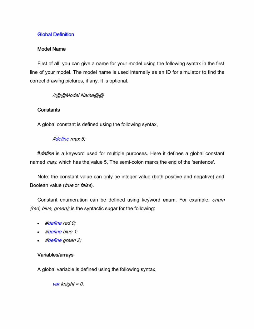
Global Definition
Model Name
First of all, you can give a name for your model using the following syntax in the first
line of your model. The model name is used internally as an ID for simulator to find the
correct drawing pictures, if any. It is optional.
//@@Model Name@@
Constants
A global constant is defined using the following syntax,
#define max 5;
#define is a keyword used for multiple purposes. Here it defines a global constant
named max, which has the value 5. The semi-colon marks the end of the 'sentence'.
Note: the constant value can only be integer value (both positive and negative) and
Boolean value (true or false).
Constant enumeration can be defined using keyword enum. For example, enum
{red, blue, green}; is the syntactic sugar for the following:
#define red 0;
#define blue 1;
#define green 2;
Variables/arrays
A global variable is defined using the following syntax,
var knight = 0;

where var is a key word for defining a variable and knight is the variable name.
Initially, knight has the value 0. Semi-colon is used to mark the end of the 'sentence' as
above. We remark the input language of PAT is weakly typed and therefore no typing
information is required when declaring a variable. Cast between incompatible types may
result in a run-time exception. A fixed-size array may be defined as follows,
var board = [3, 5, 6, 0, 2, 7, 8, 4, 1];
where board is the array name and its initial value is specified as the sequence, e.g.,
board[0] = 3. The following defines an array of size 3.
var leader[3];
All elements in the array are initialized to be 0.
Note for multi-dimensional array: PAT supports multi-dimensional arrays by
converting them into one dimensional array. You can declare and use multi-dimensional
arrays as follows. The only restriction is that you cannot assign multi-dimensional array
constant to multi-dimensional arrays variables. To initialize a multi-dimensional array,
you need to do it explicitly in some events.
var matrix[3*N][10];
var matrix[1][6] = 3;
Variable range specification: users can provide the range of the variables/arrays
explicitly by giving lower bound or upper bound or both. In this way, the model checkers
and simulator can report the out-of-range violation of the variable values to help users to
monitor the variable values. The syntax of specifying range values are demonstrated as
follows.
var knight : {0..} = 0;
var board : {0..10} = [3, 5, 6, 0, 2, 7, 8, 4, 1];
var leader[N] : {..N-1}; //where N is a constant defined.

Array Initialization: To ease the modeling, PAT supports fast array initialization using
following syntax.
#define N 2;
var array = [1(2), 3..6, 7(N*2), 12..10];
//the above is same as the following
var array = [1, 1, 3, 4, 5, 6, 7, 7, 7, 7, 12, 11, 10];
In the above syntax, 1(2) and 7(N*2) allow user to quickly create an array with same
initial values. 3..6 and 12..10 allow user to write quick increasing and decreasing loop to
initialize the array.
User defined type: To ease the modeling, PAT allows users to define any data
structures and use them in PAT models. The following shows the syntax.
var <Type> x ; //default constructor of Type class will be called.
var <Type> x = new Type(1, 2); //constructor with two int parameters will be
called.
Hidden variable: To simplify the model, PAT introduces the hidden variables which
can be used as normal variables. The only difference is that hidden variable is a kind of
secondary variable, which is not included in the state details. The idea of secondary is
to use redundant .
var a; var b;
hvar difference; //secondary variable to store the difference between a and b.
Channels
In TA module, process can synchronize over channel. A normal channel is declared
as follows,
channel c ;

where channel is a key word for declaring channels only, c is the channel name, the
buffer size of the channel is 1.
channel c[5] ;
where c is an array of channels, with the array size is 5. The concrete channel
depends on the current valuation which is the value of the array index.
Propositions
In addition, the key word #define may be used to define propositions. For instance,
#define goal x == 0;
where goal is the name of the proposition and x == 0 is what goal means. A
proposition name is used in the same way as global constant is used. For instance,
given the above definition, we may write the following,
if (goal) { P } else { Q };
which means if the value of x is 0 then do P else do Q. We remark that propositions
are the basic elements of LTL formulae.
Clocks
A clock may be a variable or an array. All the clocks progress synchronously and
real-time constraints are captured by explicitly setting/resetting clock variables. A clock
may be defined as follows:
clock x; //clock is a variable.
clock y[3]; //clock is an array.
System Definition
A system is defined as an equation in the following syntax,

P(x1, x2, ...,xn) = Exp;
where P is the system name, x1, ..., xn is an optional list of system parameters and
Exp is a process expression which is a process defined as a timed automaton or the
interleaving processes that are defined as timed automata. The process expression
determines the computational logic of the system. A system without parameters is
written either as P() or P
For example, a system Sys can be defined in such following ways:
Sys = P; //P is a defined processes without parameters.
Sys = Q(1); //Q is a defined processes with a parameter.
Sys = P() ||| Q(0); //Two interleaving processes.
where ||| denotes interleaving. Both P and Q may perform their local actions without
referring to each other. Notice that P and Q can still communicate via shared variables
or channels. The generalized form of interleaving is written as,
||| x:{0..n} @ P(x);
Assertions
TA module supports all assertions such as deadlock freeness, reachability, the full
set of Linear Temporal Logic (LTL) in CSP Module.
[TOP]
3.6.1.2 3.6.1.2 Process Definitions
In TA module, a system is modeled as a network of several processes interleaving
with each other.

It provides an easy way to create a process by drawing the operations of the
process. Each process is an automaton where a location is a snapshot of the process
and an edge is used to describe a transition from one location to another.
An edge includes five parts.
First, the Event is the name of the action making the process to change.
Second, the Clock Guard is the timed constraint of transition execution.
Third, the Transition Guard is the condition of the action to happen.
Next is the Program which is the description of the action. It defines what the new
state of the process from the current state is if this action is trigered.
Finally, Reset Clocks is set the clock to zero. In this manual we will use the
Transition and Link interchangeably. The Transition is actually represented a real link in
the canvas.
[TOP]
3.6.1.2.1 Drawing
The system editor has two parts Navigation Tree and Canvas . Navigation Tree is
used to access the editor of the system declarations and processes. The canvas is used
to edit the processes.
[TOP]
3.6.1.2.1.1 Navigation Tree
The Navigation Tree is shown in the left panel of the system editor. It is used for
accessing the global definition and process definitions. A node in the tree can be double
clicked to view and edit.

The root of the navigation tree is named TA Model. The sub node Declaration is
used for declarations of global variables, systems, and assertions. The next sub node is
Processes. It is the collection of processes which can be included to the certain system.
Please refer to the Global Definition to know how to define a system.
There are 3 items in the Navigation Tree menu. Just right click to acces the menu.
1. Add Process: Right click on sub node Processes to add a new process.
2. Delete Process: Right click on a node of a process to delete it.
3. Process Details: Right click on a node of a process to edit the name, and parameter
of that process.
[TOP]

3.6.1.2.1.2 Canvas
The right panel of the system editor is used for drawing the process. There are currently four drawing functions named Add New State, Delete, Add Link, Export Drawing as Bitmap.
1. Add New State : This button is used to create a new state. Choose this button
and click anywhere in the canvas. Beside this way, a new state can be added
from the context menu in the canvas by right click in the canvas and choose New
State.
2. Delete : Selecting this button will delete all the currently selected items
including states, links, nails.
3. Add Link : This tool is used to create a new link connecting two states. Choose
this tool first and then choose two states to be connected. Between choosing two
states, if you click anywhere in the canvas, a new nail will be automatically added
to the screen.
4. Export Drawing as Bitmap : Export the current canvas to a bitmap. However,
the program does not accept that bitmap as an input of the program.
There are some useful hotkeys supported in the TA canvas:
1. Ctrl-Z: Undo to the last state before your change.
2. Ctrl-Y: Redo to the last Undo
3. Delete: Delete the selected items in the canvas.
For users with a mouse, the left mouse is used to select an item and the right mouse
is used to access the item's context menu. User can select multiple items by dragging
the mouse pointer to create a selection around the outside of all the items to be
included.

[TOP]
3.6.1.2.2 State
A state is a snapshot of the process. A state has four properties.
Name: the name of the state. It is used to distinguish states. Two states having
the same name are actually a state representing the same snapshot of the
process.
Initial: a boolean property of state. A state is initial then it is the starting point of
the process.
Clock Invariant: an expression that is a conjunction of conditions of the form x<e
or x<=e where x is a clock

reference and e evaluates to an integer. When the clock value violates the
invariant, the next transition must involve an edge from this state.
Urgent: a boolean property of state. Urgent state freezes time; i.e. time is not
allowed to pass when a process is in an urgent state.
Commited: a boolean property of state. Commited state freezes time.
Furthermore, if any process is in a committed state, the next transition must
involve an edge from one of the committed states.
There are some actions which can do with State:
Create State: Select the Add New State function and click anywhere in the
canvas to create new state. Another way is to create new state from the canvas's
context menu by making right click on the canvas and selecting New State.

Delete State: There are also two ways to delete a state. First is select the state
then select the Delete function. Second is delete the state from that state's
context menu.
Move State: Select the state then drag the mouse to the place you want. Then
the state will be moved to that position.
Edit Name: Double click on the state to open the State Editing Form dialog.
There you can edit the state's name.
Edit Clock Invariant: Double click on the state to open the State Editing Form
dialog. There you can edit the state's clock invariant.
Set Initial: Select the initial state then set that property from the state's context
menu.
Set Urgent: Select the state then set that property from the states's context menu
or double click on the state to open the State Editing Form dialog and then select
the Urgent choice.
Set Commited: Select the state then set that property from the states's context
menu or double click on the state to open the State Editing Form dialog and
then select the Commited choice.
[TOP]
3.6.1.2.3 Transition
A transition is used to describe how the state of the process changes as the result of
some action of the process. It is composed of six parts.
Selections non-deterministically bind a given identifier to a value in a given
range. The other parts of the transition are within the scope of this binding.
Event is the name of the action making the process to change. Processes can
also synchronize over channels.
Clock Guard is the timed constraint of transition execution.
Transition Guard, a boolean expression, is the condition of the action to happen.

Program is the description of the action. It defines updated information from the
current state if this action is trigered. It is a sequence of command and may
contain while-loops, if-then-else.
Reset Clocks is setting the clock to zero.
The transition label is represented as below: select : selections clocks : <clock
guard>[transition guard]event{program}clockreset: clock. A selection binds a variable,
which appears in clock guard, transition guard, event, program or clock reset parts, in a
given range. The evaluation order of the transition is in the following: first, the transition
guard is checked, followed by the clock guard. When both guards are valid, the event
occurs, in the meantime, the program is updated and the clock is reset. If transitions
labelled with complementary actions over a common channel, the evaluation order of a
channel likes the following:
1. channel output guard evaluation and checking
2. channel output clock guard evaluation and checking
3. channel output channel name evaluation
4. channel input channel name evaluation

5. channel input guard evaluation and checking
6. channel input clock guard evaluation and checking
7. channel output program evaluation
8. channel input program evaluation.
In the above picture, the transition from state Occ to state Free is defined as select :
e:{0..N-1} [e == queue.First()] leave[e]? {queue.Dequeue();}, where queue is an
instance of data type Queue defined as a class in C# language, First() and Dequeue()
are functions defined in the Queue class. The range of variable e is from 0 to N-1, and
the value of e in the transition guard and event should also be in this scope. If Boolean
expression e== queue.First() returns true, then if processes can synchronize over
channel leave[e] (value of e should be the same in the transition guard), in this case,
event leave[e]! occurs, followed by the execution of program queue.Dequeue().
There are some actions which can do with the Transition:
Create Transition: Select the Add Link function then select the first state and the
second state. Between selections of the two states, you can click in the canvas to
create a new Nail. Nail is a small dot in yellow color. It is used to divide the
transition in segments.
Delete Transition: Select the link then click the Delete function or select Delete
function from that link's context menu.
Create Nail: Right click on the link and select New Nail.
Delete Nail: Select the Nail then select the delete function from the toolbar or its
context menu.
Move Nail: Select the Nail and drag the nail to the desired position.

[TOP]
3.6.1.3 3.6.1.3 Grammar Rules
Declaration
: (specBody)*
;
specBody
:library
|letDefintion
|assertion
|define
|channel

|definition
;
library
:'#' 'import' STRING ';'//import the library by full dll path or DLLname under the Lib folder
;
letDefintion
:'var' ID ('<' datatype=ID '>')?variableRange? ('=' expression)?';'//user defined datatype is
supported using<type>
|'var' ID variableRange? '=' recordExpression ';'
|'var' ID ('[' expression ']')+ variableRange? ('='recordExpression)?';'//multi-dimensional array
issupported
| ('clock') ID ('[' expression ']')?';'
;
variableRange
:':' '{' additiveExpression?'..' additiveExpression? '}'
;
recordExpression
: '[' recordElement (','recordElement)* ']'
;
recordElement
:e1=expression('(' e2=expression ')')?
|e1=expression'..'e2=expression
;
assertion
:'#' 'assert' definitionRef
(
('|=' ( '(' | ')' | '[]' | '<>' | ID | STRING | '!' | '?' | '&&' |'||' | '->' | '<->' | '/\\' | '\\/' | '.' | INT )+ )
|'deadlockfree'
|'nonterminating'
| 'divergencefree'
|'deterministic'
|'reaches' ID withClause
|'refines' definitionRef
|'refines' '<F>'definitionRef
|'refines' '<FD>' definitionRef
)
';'
;
withClause
:'with' ('min' | 'max') '(' expression')'
;
definitionRef
:ID ('('')')?
;
define: '#' 'define' ID INT ';'

|'#' 'define' ID ('true' | 'false') ';'
|'enum''{' ID (',' ID)*'}'';'
| '#' 'define' ID conditionalOrExpression ';'
;
block :'{'statement* expression? '}'
;
statement
:block
|localVariableDeclaration
|ifExpression
|whileExpression
|expression ';'
|';'
;
localVariableDeclaration
: 'var' ID ('=' expression)? ';'
|'var' ID '=' recordExpression ';'
;
expression
:conditionalOrExpression ('=' expression)?
;
conditionalOrExpression
:conditionalAndExpression ( '||' conditionalAndExpression )*
conditionalAndExpression
:equalityExpression ( '&&' equalityExpression)*
;
equalityExpression
:relationalExpression( ('==' | '!=') relationalExpression)*
;
relationalExpression
:additiveExpression ( ('<' | '>' | '<=' | '>=') additiveExpression)*
;
additiveExpression
:multiplicativeExpression ( ('+' | '-') multiplicativeExpression)*
;
multiplicativeExpression
:unaryExpression ( ('*' | '/' | '%' ) unaryExpression)*
;
unaryExpression
:'+' unaryExpression
|'-' unaryExpression
| '!'unaryExpressionNotPlusMinus
| unaryExpressionNotPlusMinus'++'
| unaryExpressionNotPlusMinus '--'
| unaryExpressionNotPlusMinus

;
unaryExpressionNotPlusMinus
:INT
|'true'
|'false'
|'call' '(' ID (',' conditionalOrExpression)* ')'
| newID '('(conditionalOrExpression ',' conditionalOrExpression)*)?')'
|ID '.' ID '('(conditionalOrExpression ',' conditionalOrExpression)*)?')'
| arrayExpression '.' ID '(' (conditionalOrExpression (','conditionalOrExpression)*)? ')'
|arrayExpression
|'(' conditionalOrExpression ')'
|ID
;
arrayExpression
: ID('[' conditionalOrExpression ']')+
;
ifExpression
:'if' '(' expression ')' statement ('else'statement)?
;
whileExpression
:'while' '(' expression ')' statement
;
channel
: 'channel' ID ('[' expression ']')? ';'
;
definition
:ID'=' interleaveExpr ';'
| 'Process' STRING('(' (ID (',' ID )*)? ')')?'['STRING ']' ':'stateDef+ transition* ';'
;
stateDef
: 'State:' STRING clockConstraints? '[U]'? '[C]'?
;
transition
:STRING '--' select? clockConstraints? ('[' conditionalOrExpression
']')?'##@@'eventM'@@##'(block)?
clockRestExpression?'-->' STRING
;
interleaveExpr
:indexedInterleave ( ('|||' indexedInterleave)+)
;
indexedInterleave
:atom
| '|||' (paralDef(';' paralDef )*)'@'atom
| '('!indexedInterleave ')'
;

paralDef
: ID ':' '{' additiveExpression (',' additiveExpression)*'}'
| ID ':' '{'additiveExpression '..' additiveExpression'}'
;
select
:'select' ':' (paralDef (';' paralDef )*)
;
clockConstraints
: 'clocks' ':' '<' clockConstraint ('&&' clockConstraint)*'>'
;
clockConstraint
: additiveExpression ('<='|'<'|'=='|'>'|'>=')additiveExpression
;
clockRestExpression
: 'clockreset' ':' unaryExpressionNotPlusMinus (','unaryExpressionNotPlusMinus )*
;
atom
:ID('(' (expression(',' expression )*)?')')?
;
eventM
:ID ( '.'additiveExpression)*
| 'tau'
| ID '!'
| ID '?'
;
ID
: ('a'..'z'|'A'..'Z'|'_')('a'..'z'|'A'..'Z'|'0'..'9'|'_')*
;
STRING
:'"' (~('"') )* '"'
;
WS
:(''|'\r'|'\t'|'\u000C'|'\n')
;
INT
: ('0'..'9')+
;
COMMENT
:'/*' ( : . )* '*/'
;
LINE_COMMENT
: '//' ~('\n'|'\r')* '\r'?'\n'
;
[TOP]

3.6.2 3.6.2 TA Module Tutorial
In this section, we illustrate the TA module's modeling language with the Fischer's
Protocol Example, Railway Control System Example and CSMA/CD Protocol Example.
[TOP]
3.6.2.1 3.6.2.1 Fischer's Protocol
Fischer’s protocol we examined here is a mutual exclusion protocol designed for n
processes. It only assumes atomic reads and writes to a shared variable (when the first
mutual exclusion protocols were developed in the late 1960s all exclusion protocols
were of the "shared variable kind", later on researchers have more concentrated on the
"semaphore kind" of protocol). Mutual exclusion in Fischer's Protocol is guaranteed by
carefully placing bounds on the execution times of the instructions, leading to a protocol
which is very simple, and relies heavily on time aspects.
The global declaration part
////////////////The Model//////////////////
#define k 2;
#define Idle -1;
#define N 4;
var id = Idle;
var count = 0;
clock x[N];
In this example, we define N as a constant tha represents four processes competing
for the shared variable. Clock x[N] is an array which record the clock value of each
process during the execution. Constant k constranis every process must finish their
request within k time slots. Idle denotes the shared variable is not been used. Variable
id records the shared variable state, initial, it's idele. Variable count records the nunber

of processes that has got the shared variable and it has to be no more than one all the
time.
The process definition part
Process P with parameter i:
The whole system is defined as follows:
System = ||| y:{0..N-1} @P(y);
The asserstion part
////////////////////////////////////////////////////////////////////////////////////
//verifying mutual exclusion by reachability analysis
#define MutualExclusionFail count > 1;
#assert System reaches MutualExclusionFail;

//deadlock checking
#assert System deadlockfree;
//verifying responsiveness by LTL model checking
#define request id != Idle;
#define accessCS count > 0;
#assert System |= [](request -> <>accessCS);
[TOP]
3.6.2.2 3.6.2.2 Railway Control System
In this example, we model a railway control system to automatically control trains
passing a critical point such as a bridge. The idea is to use a computer to guide trains
from several tracks crossing a single bridge instead of building many bridges.
Obviously, a safety-property of such a system is to avoid the situation where more than
one train are crossing the bridge at the same time.
For more details about this example, see [WangPD94].
The global declaration part
////////////////The Model//////////////////
#import "PAT.Lib.Queue";
//number of trains
#define N 4;
channel appr[N];
channel go[N];
channel leave[N];

channel stop[N];
var<Queue> queue;
clock x[N];
clock y;
In this example, we import the external C# library to use the queue functions.
Constant N represents the nunber of trains. We define arrays of channels to represent
the status of the N trains. Clock x[N] is an array which record the clock value of each
train during the execution.
The process definition part
Train Process with paramenter i:

Gate process:

The whole system is defined as follows:
System = ||| z:{0..N-1}@Train(z) ||| Gate;
The asserstion part
////////////////////////////////////////////////////////////////////////////////////
#assert System deadlockfree;
//Whenever a train approaches the bridge, it will eventually cross.
#assert System |= []("appr[1]" -> <> "leave[1]"); //Notice: channel should be specified
as a string eclosed within a pair of " ".
//overflow: There can never be N elements in the queue (thus the array will not
overflow).
#define overflow (queue.Count()> N);
#assert System reaches overflow;
[TOP]

3.6.2.3 3.6.2.3 CSMA/CD Protocol
In a broadcast network with a multi-access bus, the problem of assigning the bus to
only one of many competing stations arises. The CSMA/CD protocol (Carrier Sense,
Multiple-Access with Collision Detection) describes one solution. Roughly, whenever a
station has data to send, if first listens to the bus. If the bus is idle (i.e., no other station
is transmitting), the station begins to send a message. If it detects a busy bus in this
process, it waits a random amount of time and then repeats the operation.
The global declaration part
////////////////The Model//////////////////
#define N 4; //number of stations
channel begin;
channel end;
channel busy;
channel cd[N];
var k = [-1(N)]; //record state of the station, 0: sending the message
var j = 0; //used to broadcast the collision messgae
clock x; //the clock for bus
clock y[N]; //the clock for the station
In this example, we define N as a constant tha represents four stations competing
for the bus. channel begin represents that station begins to send messages; channel
end represents that the station completes the transmission; channel busy represents
that one station is sending the messages on the bus; channel cd[N] is an array of
channels, representing that the ith station receives a collision.
The process definition part
Bus Process:

Station Process with paramenter i:

In this example, when process Bus is in the bus_collision state, and process
Station(0) is in the sender_retry state, the next execution is that two
processes synchronise by channel cd, the evaluation order of the channel cd likes the
following:
1. channel cd[j]! output clock guard (x<26) evaluation and checking
2. channel cd[j]! output channel name evaluation (j)
3. channel cd[i]? input channel name evaluation (the value of i is 0)
4. channel cd[i]? input clock guard (y[i]<52) evaluation and checking
5. channel output program (j=j+1) evaluation
The whole system is defined as follows:
CSMACD = (|||m :{0..N-1} @ Station(m)) ||| Bus;
The asserstion part
////////////////////////////////////////////////////////////////////////////////////
#assert CSMACD deadlockfree;
[TOP]
3.7 3.7 NesC Module
Sensor network applications are expected to perform critical tasks unattendedly for a
long period, thus it is important to verify their reliability and correctness. Currently
common programming languages, e.g. NesC, and platforms, e.g. TinyOS, for sensor
networks adopt the low-level programming style. Although such designs are able to

provide fine-grained control over the underlying resource constraints, they are difficult
for human to comprehend, maintain, debug and verify sensor network applications.
PAT is developed to apply model checking techniques to the sensor network domain
by this NesC module. The NesC module of PAT is created to automatically analyze
behaviors and verify properties of TinyOS applications implemented in NesC. NesC
programs are parsed to LTS semantic models, upon which the behaviors of TinyOS
applications are analyzed and their properties are verified. The tool can assist program
developers to analyze, simulate and verify their code, consequently improving the
correctness and reliability of sensor network applications.
Currently, the implementation of NesC module follows the language features of
NesC, and the execution model of TinyOS model, which are presented in the book
TinyOS Programming by Philip Levis. Most syntax of the NesC language is supported
now. Our approach is to generate Label Transition System (LTS) from nesC source
code, and then explore the state space of the LTS to verify whether it satisfies certain
properties.
Important notice: NesC module only supports application of TinyOS 2.x.
PAT is extended with this NesC module to automatically generate LTS semantic
model from NesC programs, with a graphical behavior analysis interface (Simultor) and
an interface for verifying various properties (Model Checker). The following figure shows
the architecture of the NesC module in PAT.

Firstly, NesC source code is input to the NesC Process Generator, which generates
NesC processes, with supports from the static NesC process library of TinyOS
components; secondly, LTS Generator produces the corresponding LTS model; finally,
execution traces of the resultant LTS are displayed via the simulator, and its the state
space is explored by model checking algorithms to verify user-specified properties via
the model checker.
[TOP]
3.7.1 3.7.1 Language Reference
In this section, we illustrate the language features of NesC, including the
concepts of interface, module, and configuration. In addition, the TinyOS library is
discussed, which is provided in PAT as hardware abstractions and system services for
NesC programs. Further, the assertion annotation language which is used to specify
various properties as verification goal is presented.

3.7.1.1 Drawing a Sensor Network
A graphical editor is provided for
drawing a sensor network
editing each sensor to configure the NesC program running on it
editing verification goals (i.e., assertions)
3.7.1.2 The NesC Language
The extention of NesC programs ".nc" is supported here. In addition, users are
allowed to provide ".h" files within their NesC source code files. We tried to provide the
most convenience for users such that NesC programmers can easily put the same code
that is to run on real hardware to be analyzed and verified by our tool.
(A) NesC Concepts
(B) Datatypes and Data Structures
(C) Operators
(D) Statements
3.7.1.3 TinyOS Library
A NesC program always invokes functions implemented by TinyOS, thus it is
necessary to simulate the functions provided by TinyOS. We studied the source code of
TinyOS as well as supporting documents, and have manually provided a subset of the
components and interfaces pre-defined by TinyOS, which is to be used during the
analysis and verification of NesC programs. We are now in the progress to
automatically generate a complete library covering all components and interfaces of
TinyOS.
3.7.1.4 Semantic Model
The semantic model (LTS) of a NesC application is generated in PAT, based on the
language features of NesC and the execution model of TinyOS.

3.7.1.5 Assertions
The verification of NesC programs requires users to input properties in terms of
assertions in our tool. Currently, we have supports for verifying three kinds of
assertions: deadlock freeness, state reachability, and temporal properties.
[TOP]
3.7.1.1 3.7.1.1 Drawing a Sensor Network
This section shows how to creat a sensor network model for simulation and verification in PAT.
There are a few steps:
(A). Creat a new sensor network model;
(B). Add sensor nodes and links between them;
(C). Edit sensor information: assign application for running on them;
(D). Edit verification goals;
(E). Simulation;
(F). Verification.
(A) Creat a new sensor network model
From the main menu, click "File -> New -> NESC Model".

PAT will creat a sensor network model automatically, which has one sensor and the sensor is named
Sensor1.
(B) Add sensor nodes and links between them
A new sensor will be created by first clicking the green button on the Network editing panel and then
click the white panel to place the new sensor.

When a new sensor is created, it is automatically added to the list on the Sensors list on the left of the
network editing panel.
Similar, clicking the arrow button and then clicking two sensors sequentially will create a logical
link between two sensors. In PAT, a network topology is considered as a directed graph.
E.G., adding a data link between sensor1 and sensor2.

(C) Edit sensor information
One can view the details of the sensor by double click it. As shown in the following figure, when a
new sensor is created, it is assigned with "app" application by default. Note that this app program does
not really exist, so the next step is to edit the sensor information.

The table bellow explains each entry in the sensor editing form:
Entry Meaning Nullable Remark
Name Name of the sensor No Each sensor should have a unique
name, for accessing its local status.
TOS_NODE_ID The unique ID of the
sensor No
Each sensor should have a unique ID,
similar what is required in TinyOS.
Application The NesC program
running on the No
The model (.sn file) should be saved in
the same path where there are the

sensor source .nc files of the appointed NesC
program.
Sensor's
Range
The data range of
each sensor device Yes
If null, PAT will use the default data
range ([0, 1]) for sensor devices.
Buffer Size
The size of the buffer
for storing incoming
msg's
Yes If null, PAT will use the default size
(1) for each sensor.
Another way to edit a sensor is to right click it from the Sensors list, which will also open the sensor
editing form.
The top-level configuration of the NesC program assigned to a certain sensor can be viewed in PAT
editor, by double clicking the sensor from the Sensors list on the left panel.

E.G., the following shows the code of Sensor1. Sensor1 is configured to run a NesC program with
BlinkAppC being the top-level configuration/component.

(D) Edit verification goals
Double click Assertion item to switch to the assertion editor.

In the assertion editor, one can edit any number of assertions for verification. The syntax for writing
assertions can be found in 3.7.1.5 Assertions.
(E) Simulation
Clicking the Simulation button or pressing F6 will open the Simulation form.
(F) Verification
Clicking the Verification button or pressing F7 will open the Verification form.

[TOP]
3.7.1.2 3.7.1.2 The NesC Language
The development of NesC module in PAT aims at automatically analyzing,
simulating and verifying NesC programs running on TinyOS. Therefore, we tried to
support the full set of NesC syntax, including NesC structures, C-like language syntax,
etc. A NesC application can be implemented by a number of .nc files and .h files,
where .nc files define interface, module, or configuration, and .h files define some
constants and data structures. NesC code implemented in the form of .nc files and .h
files can be compiled, analyzed, simulated and verified in our tool.
(A) NesC Concepts
Interface
An nesC interface is defined as the following:
Syntax of an interface definition file
interface name {
command datatype name(datatype arg1, ...);
...
event datatype name(datatype arg1, ...);
...
}
For example, the content of file Leds.nc defines the interface Leds:
Sample Code: Leds.nc
interface Leds {
async command void led0On();
async command void led0Off();

async command void led0Toggle();
...
}
Module
A nesC module defines a lower-level component, which can be referred by a higher-
level one defined by a configuration. The syntax of a module is given as the following:
Syntax of a module definition file
module name {
uses interface name;
...
provides interface name;
...
} implementation {
datatype var, ...;
command datatype name.name(datatype arg,...){
//command implementation statements
}
...
event datatype name.name(datatype arg,...){
//event implementation statements
}
...
task void name(){
//task statements
}
...
}

For instance, the content of the file LedsP.nc defines a component named LedsP:
Sample Code: LedsP.nc
module LedsP() {
provides {
interface Init;
interface Leds;
}
uses {
interface GeneralIO as Led0;
interface GeneralIO as Led1;
interface GeneralIO as Led2;
}
} implementation {
command error_t Init.init() {
atomic {
dbg("Init","LEDS: initialized.\n");
call Led0.makeOutput();
...
call Led0.set();
...
}
return SUCCESS;
}
async command void Leds.led0On() {
call Led0.clr();
DBGLED(0);
}
async command void Leds.led0Off() {

call Led0.set();
DBGLED(0);
}
async command void Leds.led0Toggle() {
call Led0.toggle();
DBGLED(0);
}
...
}
Configuration
A configuration is the other kind of component (one kind is module) in NesC. A
configuration wires components to one another via bi-directional interfaces. In a
configuration, components are wired to one another via bi-directional interfaces. These
wiring statements are most important, because they bring all components defined
elsewhere together to be an application. Each NesC application should have a
configuration which is the top-level component and specifies the starting point of its
execution.
The syntax of a configuration is shown below:
Syntax of a configuration definition file
configuration name {
provides interface name;
...
uses interface name;
} implementation {
component name, ...;
name(.name) -> name(.name);
name(.name) <- name(.name);

name(.name) = name(.name);
...
}
(B) Datatypes and Data Structures
NesC supports the whole set of data types and structures of C language. In PAT, all
these types and structures are supported, except floating and double data.
Category Types
Primary data
type int, char, void
Integer type
int, int8_t, int16_t, int 32_t,
int64_t,
uint8_t, uint16_t, uint32_t,
uint64_t
User defined
type typedef type identifier
Enumerated
type
enum identifier {value 1, value
2, ...}
Structure struct
Pointer pointers of the supported types
in
(C) Operators
The NesC module in PAT supports all the operators of NesC, which are the same as
those of C language. The following table shows all the operators with their precedences,
description and associativity.
Precedence Operator Description Associativity

1
++ --
( )
[ ]
Suffix increment and decrement
Function call
Array subscripting
Element selection by reference
Element selection through pointer
Left to
right
2
++ --
+ -
! ~
(type)
*
&
sizeof
Prefixe increment and decrement
Unary plus and minus
Logical NOT and bitwise NOT
Type cast
Indirection (dereference)
Address-of
Size-of
Right to
left
3 * / % Multiplication, division, and modulus
(remainder)
Left to
right
4 + - Addition and subtraction Left to
right
5 << >> Bitwise left shift and right shift Left to
right
6 < <=
> >=
For relational operators less than
(LT) and less than or equal to (LE)
For relational operators greater than
(GT) and greater than or equal to (GE)
Left to
right
7 == != For relational equal to and inequal to Left to
right
8 & Bitwise AND Left to
right
9 ^ Bitwise XOR Left to
right
10 | Bitwise OR Left to

right
11 && Logical AND Left to
right
12 | | Logical OR Left to
right
13 c ? t : f Ternary conditional Right to
left
14
=
+= -=
*= /= %=
Direct assignment
Assignment by sum or difference
Assignment by product, quotient and
remainder
Right to
left
(D) Statements
Some important statements are given in the following table:
Statement Syntax
if/if-else same as C
while/do-while same as C
for same as C
command call call intf.cmd(...);
event signal signal intf.evnt(...);
task post post taskname();
[TOP]
3.7.1.3 3.7.1.3 TinyOS Library
TinyOS is implemented in NesC, as a set of interfaces and components, which
abstract hardware services and are necessary for NesC programs to execute
correctly. TinyOS is the platform which NesC programs are running upon. It provides

hardware interfaces and services including display(LED), timing(Clock & Alarm), data
transfer(UART), sensing(Photo, Temperature, ADC) and communications(Message,
Packet, Byte, RFM), as NesC interfaces and components.
TinyOS handles hardware services and its source code traverses a multiple-level
hierarchy with a number of components. And the bottom components/interfaces
program on chips directly, the semantics of which is quite different from high-level ones.
Currently, PAT focuses on the high-level behaviors of NesC applications and we have
high confidence on the reliability and correctness of TinyOS, assuming it is always
correct. Therefore, PAT comes out with a static library of NesC processes abstracting
and modeling the behaviors of components implemented by TinyOS. In summary,
several strategies and assumptions are taken into account during modeling hardware
services provided by TinyOS.
Firstly, component variables are introduced to model states of certain hardware,
although in real TinyOS those variables do not exist. This is justified in that component
variables are private and local, and introducing extra component variables will not bring
forth variable conflicts in the whole NesC program. For example, component LedsC is
an interface to turn on or off leds of a sensor node, and three component variables are
introduced to model the state (ON or OFF) of three leds respectively. As for commands
such as leds.led0On(), leds.led0Off() and others, which are turning on or off certain
leds, they are modeled as NesC processes composed of an assignment updating the
value of corresponding component variables.
Secondly, system logics of hardware services are highly abstracted, because of the
assumption that hardware has few errors. Moreover, our approach aims at helping
NesC programmers to understand their code more easily, to whom TinyOS serves like a
black-box. Therefore, for commands that implement straightforward hardware behaviors
but are presented in complicated NesC code, we make them compact and abstract with
processes updating related states and signaling corresponding events, denoting the

completion of hardware request. For example, command AMSend.send() is modeled as
process P = (post sendDone; return SUCCESS), where post sendDone posts a task
(sendDone()) which simply signals the event AMSend.sendDone().
Thirdly, process Wait models the behaviors of Timers.
For example, command Timer.startPeriodic(50) is modeled as:
while(timer == start){Wait[50];
(signal~Timer.fired())}
which signals the event Timer.fired() every 50 time units. is used here to model the
fact that exactly at the end of 50 time units, the fired event is signaled.
Currently, PAT has only provided a subset of interfaces and components of TinyOS, as
shown in the bellow table.
Service Interfaces Components
Initialization Boot, Init MainC
Timing Timer, Alarm TimerMilliC
Packet
PacketAcknowledgeme
nts,
AMPacket, Packet,
CollectionPacket
ActiveMessageC,
SerialActiveMessageC,
Communica
tion Send, Receive
AMSenderC,
AMReceiverC
Leds Display LedsC
Sensing Read, DemoSensorC,
Control SplitControl,
StdControl, RootControl MainC

Data
Structure Queue, Pool --
[TOP]
3.7.1.4 3.7.1.4 Semantic Model
Coming out soon.
[TOP]
3.7.1.5 3.7.1.5 Assertions
Our assertion annotation language includes assertions for defining deadlock
freeness, state reachability, and temporal properties. In PAT, System is a default
keyword which represents the LTS of the input NesC application. The following describe
the syntax and usage of each type of assertion, as well as the BNF of defining an
assertion in PAT.
(A) Deadlock Freeness Checking (Nontermination Checking)
Deadlock freeness (also called nontermination) is an critical and desirable property of
most sensor network applications, since scuh applications are always expected to run
unattendedly for a long period like months or even years.
Syntax of Deadlock Freeness/Nontermination Checking
#assert System deadlockfree (#assert System nonterminate)
(B) State Reachability Checking
State reachability checking is to verify whether a certain state can be reached within
finite steps of execution.

Syntax of State Reachability Checking
#assert System reaches State;
A state is defined in the following syntax, by a logical formula on variables of
components.
The following defines a state with the name State.
Syntax for difining a state
#define State ; // ¦· is a logical formula
Notice that in the following BNF, v statnds for a component-level variable (e.g.
LedsC.led0 in BlinkApp Example), and c is either a constant value or another variable.
BNF for logical formula
::= T true
| F false
| ! negation
| && conjunction
| | | disjunction
| v == c relational equal
| v != c relational inequal
| v < c relational less than
| v <= c relational less than or equal to
| v > c relational greater than
| v >= c relational greater than or equal
to

An example of state reachability checking is as follows.
Defining a state led1ON #define led1ON LedsC.led1 == 1;
Checking reachability #assert System reaches led1ON;
(C) Temporal Property Checking
A temporal property is specified by a linear temporal logic (LTL) formula, the syntax of
temporal property and LTL formula are described in the following tables, respectively.
Syntax of Temporal Property Checking
#assert System |= ;
BNF for LTL formula
- ::= T true
| F false
| p p ranges over (States U Actions)
| ! negation
| && - conjunction
| | | - disjunction
| X - next time
| F - eventually
| G - always
| U - until
Notice that (States U Actions) is the union of States, i.e. the set of states defined in by
user using the format in (B), and Actions, i.e. the set of actions.

(D) Grammar Rules of Assertions
Defining an assertion in PAT follows the BNF shown below:
assertionExpr : '#' 'assert' VAR '|=' ltlExpr ';'
| '#' 'assert' VAR 'deadlockfree' ';'
| '#' 'assert' VAR 'reaches' VAR ';'
| '#' 'assert' VAR 'reaches' eventExpr ';' ;
eventExpr : eventEle ('.' eventEle)+ ;
eventEle : BOOL | ERRORT | VAR | ZERO | NATURAL | '[' | ']' ;
ltlExpr : (ltlTokenExpr)+ ;
ltlTokenExpr : eventExpr | ltlOprExpr;
ltlOprExpr : ltlOprEle | valueExpr ;
valueExpr : VAR | ZERO | NATURAL ;
ltlOprEle : '(' | ')' | '[]' | '<>' | '&&' | '||' | '->' | '!' | '<->' | '/\\' | '\\/' ;
BOOL : 'TRUE' | 'FALSE' ;
ERRORT : 'SUCCESS' | 'FAIL' | 'ESIZE' | 'ECANCEL' | 'EOFF' | 'EBUSY'
| 'EINVAL' | 'ERETRY'| 'ERESERVE' | 'EALREADY' | 'ENOMEM' | 'ENOACK'
| 'ELAST' ;
VAR : ('a'..'z'|'A'..'Z'|'_') ('a'..'z'|'A'..'Z'|'0'..'9'|'_')* ;
ZERO : '0';
NATURAL : ('1'..'9')('0'..'9')* ;
[TOP]
3.7.2 3.7.2 nesC Module Tutorial
In this section, we use examples to illustrate how PAT can be used to faciliate the
analysis, simulation and verification of NesC applications. PAT supports simulating and
verifying both an individual sensor and a sensor network. We will illustrate both levels'
analysis via

3.7.2.1 Individual Sensor Tutorial
- BlinkApp Example
3.7.2.2 Sensor Network Tutorial
- LeaderElection Protocol
Last but not least, there are also built-in examples in PAT distribution via "Examples
-> NesC Examples". The source files of the examples can be found in PAT distribution
via /PAT_Installation/Modules/NESC, where PAT_Installation is the folder where PAT is
installed.
[TOP]
3.7.2.1 3.7.2.1 Individual Sensor Tutorial
Currently, we provide one example for illustrating the simulation and verification of an individual sensor. More examples will be added soon.
BlinkApp Example

[TOP]
3.7.2.1.1 BlinkApp Example
BlinkApp is a simple
application in the TinyOS
distribution. BlinkApp toggles the
mote LED periodically, with three
timers at different periods. The
application contains two .nc files:
BlinkAppC.nc
BlinkC.nc
The .sn file for PAT is Blink.sn,
which contains the verification goals
that are discussed in (B)Verification.
(A) Simulation
The figure on the left shows the first
few steps when simulating
BlinkApp. A square stands for a
configuration (state) of the LTS, and
an arrow is an transition between
configurations, labelled with the
corresponding action.
As an example, initially, state 1
transits to state 2 with the action
Sensor1.BlinkC.call.Timer0.startPeri
odic, which means that, component
BlinkC calls the command
startPeriodic via the interface

Timer0, which will trigger Timer0 to start timing and fire after an amount of
time. Similar are the meanings for action Sensor1.BlinkC.call.Timer1.startPeriodic and
Sensor1.BlinkC.call.Timer2.startPeriodic.
State 4 transits to state 5 with the label Sensor1.Timer0.firing, which stands for an
interrupt from Timer0 meaning that Timer0 is firing. Then Timer.fired event is
signaled. This reserves the semantics of the timing service in TinyOS.
State 5 transits to state 6 by signalling the event Timer.fired from the component
Timer0. The body of the event Timer.fired is defined by BlinkC. Therefore, state 6
transits to state 7 by the event Sensor1.BlinkC.call.Leds.led0Toggle, which is the only
statement of event Timer0.fired in component BlinkC.
In PAT, variables are introduced to model the status of leds. For example, variable
Sensor1.LedsC.led0 keeps track of the status of led0 of a mote.

(B) Verification
Users can define assertions to verify the NesC application for various properties, using
the assertion annotation language described in 3.7.1.4 Assertions. As for BlinkApp,
several assertions are defined, with states.
The following table defines three states that are used in the assertions later.
State Definition Description
#define led0ON Sensor1.LedsC.led0 == 1; Led 0 is
ON.
#define led0OFF Sensor1.LedsC.led0 == 0; Led 0 is
OFF.
#define led1ON Sensor1.LedsC.led1 == 1; Led 1 is
ON.
This table defines eight assertions for different properties of BlinkApp.
N
O. Assertion Property
1 #assert Sensor1 |= <> [] led0ON;
Led 0 will eventually always be ON,
i.e.
led 0 will finally be ON constantly.
2 #assert Sensor1 |= [] <> led0ON;
Led 0 will always eventually be ON,
i.e.
led 0 will be ON infinitely often.
3 #assert Sensor1 reaches led1ON;
The state where led 1 is ON will be
reached
within finite steps.

4 #assert Sensor1 deadlockfree; The system is deadlock free.
5 #assert Sensor1 nonterminating; The system is nonterminating.
6 #assert Sensor1 |= []<> led0OFF;
Led 0 will always eventually be OFF,
i.e.
led 0 will be OFF infinitely often.
7
#assert Sensor1 |=
[] ((led0ON -> (<> led0OFF)) &&
(led0OFF -> (<> led0ON)));
Whenever led 0 is ON it will
eventually be OFF,
and vice versa.
8 #assert Sensor1 |= [] <>
Sensor1.LedsC.led0Toggle;
Compoent LedsC toggles led 0
infinitely often.
The results of verifying BlinkCApp against the assertions defined above are as the
following figure. Notice that all properties are satisfied by BlinkApp, except the first one,
which is reasonable.

[TOP]
3.7.2.2 3.7.2.2 Sensor Network Tutorial
Currently, we provide one example for illustrating the simulation and verification of a sensor network. More examples will be added soon.

LeaderElection Protocol
[TOP]
3.7.2.2.1 LeaderElection Protocol
LeaderElection protocol is simple network consesus protol. With this protocol, eventually the sensor
with the highest TOS_NODE_ID (which is unique for each sensor) should be elected as the leader.
(To be continued.)
[TOP]
3.8 3.8 Orc Module
Service orchestration systems embrace the concept of Service Oriented Architecture
(SOA) and is gaining popularity over the time. Many of such systems support
concurrency, and it is known that concurrency bug is difficult to discover solely by
testing, thus model checking such systems is crucial.
Orc is proposed as a powerful yet elegant language for distributed and concurrent
programming which provides computational services such as distributed communication
and data manipulation via sites. With a few concurrency primitives, programmers are
able to orchestrate the invocation of sites to achieve a goal, and meanwhile, manage
timeouts, priorities, and failures. To guarantee the correctness of Orc models, effective
verification support is desirable.

The above illustrates the workflow of our approach. First, users can specify Orc
models as well as various assertion properties via the editor. The input models of
orchestration language and external services are compiled into internal representations
(i.e., LTS), based on the operational semantics of Orc. On top of that Compositional
Partial Order Reduction (CPOR) is applied. Linear Temporal Logic (LTL) assertions are
subsequently translated into Büchi automata. Users can visualize the system behaviors
via an animated simulator, or perform verification using different verifiers. If ever certain
assertions or property is violated, a counterexample will be generated which can also be
rendered in simulator.
[TOP]
3.8.1 3.8.1 Language Reference.htm
The language references is structured as follows:
3.8.1.1 The ORC Language

This section gives you an overview of Orc language.
3.8.1.2 Addon for Verification
For ease of verification, we introduce several addons to the language. This section
will give you an introduction for those addons.
3.8.1.3 Assertions
This section would introduce the assertions that are supported.
3.8.1.4 Supported Sites
This section lists the sites that are supported.
3.8.1.5 Grammar Rules
This section introduce you the complete grammar rules.
[TOP]
3.8.1.1 3.8.1.1 The ORC Language.htm
The fundamental of Orc calculus is the execution of expressions, which are built up
recursively with concurrent combinators. During execution, an expression may call sites
(i.e., external services) or publish values. The section served as the brief introduction of
the language, for complete coverage of the language, please refer to the
[ORCUserGuide].
Site
Sites are basic units of Orc language. A site can be an unreliable external service
(e.g., Google), or a predictable and well-defined local service (e.g., if). Henceforth, we
will refer the former as external site or external service and latter as local site or local
service. The simplest Orc expression is a site call M(p), where M is the service’s name

and p is a list of parameters. The effect of a site call can be response (when it returns a
value), halted (when it explicitly reports that it will never respond), or pending (neither
response nor halted). As an example, Google("Orc") calls the external service provided
by Google and its response is the search result for "Orc" by Google search engine. Site
calls are strict, which means that a site can only be called if all its parameters have
values.
Function
Like many other programming languages, functions are expressions with a defined
name and a list of parameters. When a function is called, the function body is executed
immediately if it does not make use of unbounded argument expressions, and the
argument expressions are executed in parallel with the function body.
Combinators
There are four combinators: parallel, sequential, pruning, and otherwise
combinators.
(1) Parallel Combinator (F | G)
The parallel combinator F | G defines a parallel expression, where
expressions F and G execute independently, and its published value can be the
value published either by F or by G or both of them. As an example,
Google("Orc") | Yahoo("Orc") will call Google and Yahoo site for searching "Orc"
concurrently.
(2) Sequential Combinator (F > x > G)
The sequential combinator F > x > G defines a sequential expression, where
each value published by F initiates a separate execution of G wherein x is bound
to it. The execution of F is then continued in parallel with all these executions of
G. The values published by the sequential expression are the values published

by the executions of G. As an example, (Google("Orc") | Yahoo(\Orc")) > x >
Email(addr; x) will call Google and Yahoo sites simultaneously. For each
returned value, an instance of x will be bound to it, and an email will be sent to
addr for each instance of x. Thus, up to two emails will be sent. If x is not used in
G, F >> G can be used as a shorthand for F > x > G.
(3) Pruning Combinator (F < x < G)
The pruning combinator F < x < G defines a pruning expression, where
initially F and G execute in parallel. However, when F needs the value of x it will
be blocked until G publishes a value to bind x and G terminates immediately after
that. As an example, Email(addr; x) < x < (Google("Orc") | Yahoo("Orc")) will be
able to get the faster result for the email sending to addr. In contrast to sequential
expressions, it will publish at most one value. if x is not used in F, F << G can be
used as a shorthand for F < x < G.
(4) Otherwise Combinator (F ; G)
The otherwise combinator F ; G defines an otherwise expression, where F
executes first. The execution of F is replaced by G if F halts without any
published value. F halts if all site calls are responded or halted, and it does not
publish any more value or call any more site. As an example, in (Google("Orc") ;
Yahoo("Orc")) > x > Email(addr; x), expression Yahoo("Orc") is used as a backup
service for searching "Orc" and it will be called only if the site call Google("Orc")
halts without any result for "Orc".
Functional Core Language
Orc is enhanced with functional core language (Cor) to support various data types,
mathematical operators (e.g., 1+2), conditional expressions (i.e., if E then E else E),
etc. The complete supported syntax can be found in Section 3.8.1.4. Cor
structures are eventually translated into the fundamental syntax of Orc.

Example - Metronome
Timer can be used to execute an action periodically, e.g. polling a service on a
regular interval. Following is a function that defines a metronome, which executes an
action at regular intervals. Note that the function is defined recursively.
def metronome(t) = signal | Rtimer(t) >> metronome()
The following example publishes "tick" once per second, and publishes "tock" once
per second after an intial half-second delay. Thus the publications are "tick tock tick ... "
where "tick" and "tock" alternate each other
metronome(1000) >> "tick"
| Rtimer(500) >> metronome(1000) >> "tock"
[TOP]
3.8.1.2 3.8.1.2 Addon for Verification.htm
Sites for Verification
Global Variable
As Orc does not have a notion of global variable, in order to be able to easily assert
a global property that holds throughout the program, we extend Orc with a notion of
global variable. Global variable in Orc must prefixed by globalvar keyword, and defining
at the beginning of the program.
GUpdate Site
To assign a value to a global variable directly, a special site $GUpdate is provided.
Consider the metronome example in Section 3.8.1.1 with global variables and
$GUpdate inserted,

globalvar tickNum = 0
metronome(1000) >> $GUpdate({tickNum = tickNum + 1})>> "tick"
| Rtimer(500) >> metronome(1000) >> $GUpdate({tickNum = tickNum - 1}) >>
"tock"
we can verify whether it is possible to have two consecutive "tick"s or two
consecutive "tock"s by checking whether the system is able to reach the state satisfying
(tickNum < 0 \/ tickNum > 1).
Global Variable InitializationSometimes, global variable need to be initialized before
its use. The intialization section is declared just after the global variable declaration,
and the section is surrounded by curly bracket { }.
Consider the example below, the global variable arr is a two-element array, and it is
initialize with the value [2,1] before it is passed the the quicksort function.
globalvar arr=Array(2)
{arr.set(0,2)>>arr.set(1,1)}
def quicksort{a}= ...
quicksort(arr)
External Sites Modeling
Service orchestration systems would normally involve external services. External
services would incur, furthermore, there might be cases where communication halted
unexpectedly, or the services simply non-responsive.
Following is the syntax that used to model the external site,
ExternalSite SiteName(Args)[haltAllow{Delay}]{DelayTups}
SystemVarDecls
{SystemVarInits}

ORCExpression
EndSite
where ExternalSite and EndSite denotes the start and end of the external site
modeling. SiteName is the service name of the external site; Args is a set of arguments
for the site; haltAllow is an optional tag to specify whether to model the halting behavior,
and Delays is a set of natural numbers which denotes the possible delays before
halting. DelayTups is a set of tuple (t1,t2) which is used to specify all possible
communication delays of the external service. The domain of t1 and t2 is natural
numbers. t1 is the forward trip delay, which is used to specify the communication delay
for the service call to reach the external services plus the processing time needed just
before the internal storage of external services is updated. For simplicity of modeling,
internal storage of external services are assumed to be updated instantaneously at time
t1 and if there are multiple internal storages to be updated, we assumed all are updated
at the same time. t2 is the return trip delay, which is used to specify the processing time
of the external services just after the update of internal storage plus the delay of
returned value traveling back from the external service. Thus, the total roundtrip delay is
t1 + t2. DelayTups also allows a special "inf "(infinity delay) symbol, which is used to
denote the non-responsive behavior. SystemVarDecl is a list of system variable
declarations, which is used to model the global internal storage for the stateful external
service. All the system variable declarations are required to start with the systemvar
keyword. SystemVarInits is the section that initialize the declared system variables,
and the section is surrounded by curly bracket {} just like global variable
intialization.ORCExpression is the body of the external site modelling and it is used to
specify the output value of external site with respect to the input arguments Args.
Example - Auction Service
ExternalSite Auction(x)[haltAllow{1, 2}]{(1,1), inf} =
systemvar AuctionList = Buffer()
{AuctionList.put("1")}

(x > ("post", item) > AuctionList.put(item)
|
x > "getNext" > AuctionList.getnb()
EndSite
The above syntax specifies an Auction external site. AuctionList is started with a
value "1".
Assume argument x=("post", 100), the possible behaviors are
A. After 1 time unit, the external services updated the Auction-List with the value
100, and spent another 1 time unit for the signal value to come back to the caller;
B. After 1 time unit, the system is halted;
C. After 2 time units, the system is halted;
D. The service call is non-responsive.
[TOP]
3.8.1.3 3.8.1.3 Assertions.htm
Reasoning on System Bahaviour
Deadlock-freeness
Given a system in Orc, the following assertion asks whether the System is deadlock-
free or not.
#assert System deadlockfree;
Reachability
Given a system in Orc, the following assertion asks whether P() can reach a state at
which some given condition is satisfied.
#assert P() reaches cond;

Consider the metronome example as described in section 3.8.1.1 with GUpdate and
#define section added
globalvar tickNum = 0
metronome(1000) >> $GUpdate({tickNum = tickNum + 1})>> "tick"
| Rtimer(500) >> metronome(1000) >> $GUpdate({tickNum = tickNum - 1}) >>
"tock"
#define consecutiveTickOrTock (tickNum < 0 || tickNum > 1)
The #define section defines a condition named as consecutiveTickOrTock which
represents the condition such that tickNum is either smaller than 0 or larger than 1. The
following assertion queries that whether the System is possible to reach the condition
consecutiveTickOrTock.
#assert System reaches consecutiveTickOrTock;
Linear Temporal Logic
In PAT, we support the full set of LTL syntax. Given a system in Orc, the following
assertion asks whether the system satisfied LTL property F
#assert System |= F;
where F is an LTL formula whose syntax is defined as the following rules,
F = "p" | prop | [] F | <> F | X F | F1 U F2 | F1 R F2
where p is a publish value, prop is a pre-defined proposition, [] reads as "always"
(also can be written as 'G' in PAT), <> reads as "eventually" (also can be written as 'F' in
PAT), X reads as "next", U reads as "until" and R reads as "Release" (also can
be written as 'V' in PAT). Consider the metronome example (Section 3.8.1.1), we can
query whether the system is always not possible to reach a state that satisfies
consecutiveTickOrTock with the following assertion

#assert System |= []!consecutiveTickOrTock ;
we can also query whether the system can always eventually publish value "tick" in
the future with the following assertion
#assert System |= []<>"tick";
Reasoning on Non-Reponsive Sites
A non-responsive service is normally up to the operating system to decide when to
end the connection. The undeterministic waiting time is not always desirable especially
in time-critical system. In time-critical system, the system might expect the value to be
received within certain time units, or otherwise, some alternative remedy actions will be
done. In such case, proper timeout mechanism need to be introduced to end the non-
responsive service if it takes longer than the t time units. Orc has provided such timeout
mechanism. As an example, the Orc expression x < x < (Google("Orc") |
Rtimer(5) >> ...) will end the Google service if it does not return within 5 time units,
where ... denotes the necessary remedy actions. Nonetheless, it is possible that some
external services in the system are leaved unhandled for their potential non-responsive
behaviour due to human errors. We provide two kinds of assertions for the user to find
out unhandled non-responsive site call in their system. The assumption for the checking
is that, there is no external parties like operating system that will help to end the non-
resposive site call. A special site NRS is used to internally simulate the behaviour of
non-reponsive site.
Non-Responsive Site Deadlock (NRSDeadlock)
This is to check whether the non-responsive site call can cause the system
deadlock. The following assertion asks whether the system is free of NRSDeadlock
behaviour,
#assert System nrsdeadlockfree;

Non-Responsive Site Cycle (NRSCycle)
This is to check whether there exists non-responsive site call that does not cause
the system deadlock, but it is always unhandled. Consider expression (S1 >> S2) | S3,
if S1 is non-responsive external site call and S3 is always executable (i.e., deadlock-
free), the system will still be running smoothly, since S1 and S3 is run on different
threads or processors. Nonetheless, S2 will never be run. The following assertion asks
whether the system is free of NRSCycle behaviour,
#assert System nrscyclefree;
[TOP]
3.8.1.4 3.8.1.4 Supported Sites.htm
For the details of usage of the sites that are listed here, please refer to
[ORCUserGuide].
1. Fundamental sites and operators
let, if, (op)
2. General-purpose supplemental data structures.
Site Method
Semaphore acquire, acquirenb, release
Buffer get, getnb, put
SyncChannel get, put
Ref read, write
Array fill, get, set, length
Counter inc, dec, onZero
Set add, contains, remove, size
3. Relative Timer

Rtimer
[TOP]
3.8.1.5 3.8.1.5 Grammar Rules.htm
Exp ::= (Expression)
(Ext)* (Gvar)* {E} E (Define)* (Assert)*
Ext ::= (External Site)
ExternalSite X(P,..,P)([haltAllow{TimeREx}])?{TimeEx} (external site header)
(SVar)* (system variable declaration)
{E} (system variable initialization)
E (external site body)
EndSite (external site footer)
TimeREx ::= (Time Range Expression)
(Integer,Integer) (time range tuple)
| inf (infinity/non-response)
TimeEx ::= (Time Expression)
Integer,...,Integer (time List)
GVar ::= (Global Variable)
globalvar X(=P)? (global variable declarartion)
SVar ::= (System Variable)
systemvar X(=P)? (system variable declarartion)
E ::= (ORC Expression)

C (constant value)
| X (variable)
| stop (silent expression)
| ( E , ... , E ) (tuple)
| [ E , ... , E ] (list)
| E G+ (call)
| op E (prefix operator)
| E op E (infix operator)
| if E then E else E (conditional)
| E >P> E (sequential combinator)
| E | E (parallel combinator)
| E <P< E (pruning combinator)
| E ; E (otherwise combinator)
G ::= (Argument group)
( E , ... , E ) (arguments)
| . (field field access)
C ::= (Constant)
Boolean
| Integer
| String
| signal
| null
X ::= (Variable)
Identifier

D ::= (Declaration)
val P = E (value declaration)
| def X( P , ... , P ) = E (function declaration)
P ::= (Pattern)
X (variable)
| C (constant)
| _ (wildcard)
| ( P , ... , P ) (tuple pattern)
| [ P , ... , P ] (list pattern)
| P : P (cons pattern)
Define:= (Condition Definition)
#define X (E)
Assert:= (Assertion)
#assert System
(deadlockfree (deadlock-freeness check)
| reaches X (reachability check)
| |= LTL (ltl check)
| nrsdeadlockfree (nrsdeadlock-freeness check)
| nrscyclefree) (nrscycle-freeness check)
LTL:= (LTL Expression)
"C" (publish value)
| X (predefined condition)
|[] LTL (always)
|<> LTL (eventually)

|X LTL (next)
|LTL U LTL (until)
|LTL R LTL (release)
[TOP]
3.8.2 3.8.2 ORC Module Tutorial.htm
In this section, we illustrate the RTS module's modeling language using a number of
examples.
Metronome
Concurrent Quicksort
Auction Management
[TOP]
3.8.2.1 3.8.2.1 Metronome.htm
Metronome executes an action at regular intervals, e.g., polling a service on a
regular interval.
globalvar tickNum=0
The above defines a global variable tickNum, which is used to record the number of
continuous "tick".
def metronome(t) = signal | Rtimer(t) >> metronome(t)
The above defines a metronome where it publishes signal every t time unit.

metronome(1000) >> $GUpdate({tickNum=tickNum+1}) >> "tick"
| Rtimer(500) >> metronome(1000) >> $GUpdate({tickNum=tickNum-
1}) >>"tock"
The above publishes "tick" once per second, and publishes "tock" once per second
after an intial half-second delay. Thus the publications are "tick tock tick ... " where "tick"
and "tock" alternate each other.
#define consecutiveTickOrTock (tickNum < 0 || tickNum > 1)
The above defines a condition named as consecutiveTickOrTock which represents
the condition such that tickNum is either smaller than 0 or larger than 1.
#assert System deadlockfree;
The above checks whether the system is deadlock-free.
#assert System |= []<>"tick" && []<>"tock";
The above checks whether the system can always eventually publish "tick" and
always eventually publish "tock".
#assert System |= []!consecutiveTickOrTock;
The above checks that whether the system always not satisfies the condition
specified by consecutiveTickOrTock.
#assert System reaches consecutiveTickOrTock;
The above checks that whether the system can reaches the condition specified by
consecutiveTickOrTock.
[TOP]
3.8.2.2 3.8.2.2 Concurrent Quicksort.htm

Concurrent Quicksort is a variant of classic quicksort algorithm which emphasizes its
concurrent perspective.
globalvar arr=Array(3){arr.set(0,3)>>arr.set(1,2)>>arr.set(2,1)}
The above defines a global variable arr of type array, which has [3,2,1] as its initial
value.
def quicksort(a) =
def swap(x, y) = a.get(x) >z> a.set(x,a.get(y)) >> a.set(y,z)
def part(p, s, t) =
def lr(i) = if i < t && a.get(i) <= p then lr(i+1) else i
def rl(i) = if a.get(i) > p then rl(i-1) else i
(lr(s), rl(t)) >(s', t')>
( if (s' + 1 < t') >> swap(s', t') >> part(p, s'+1, t'-1)
| if (s' + 1 = t') >> swap(s', t') >> s'
| if (s' + 1 > t') >> t'
) def sort(s, t) =
if s >= t then signal
else part(a.get(s), s+1, t) >m>
swap(m, s) >>
(sort(s, m-1), sort(m+1, t)) >>
signal
sort(0, a.length()-1)
The above defines the quicksoft function. Its details can be found at [AQDKJM09].
quicksort(arr)
The above input the global variable arr for quicksorting.
#define sorted (arr.get(0)<arr.get(1) && arr.get(1)<arr.get(2))

The above defines a condition named as sorted which represents the situation
where the number in the array is sorted in ascending order.
#assert System |= (<>sorted) && (sorted->[]sorted);
The assertion above specifies that eventually the array will be sorted, and once the
array is sorted it will remain sorted.
[TOP]
3.8.2.3 3.8.2.3 Auction Management.htm
Auction Management [MAJM10] is a simplified online auction management
application that manages posting new items for auction, coordinates the bidding
process, and announces winners.
ExternalSite MaxBidSite(x){(1,1)}=
def MaxBid(bidList,max,maxBidder)=
bidList>[]> (maxBidder,max)
| bidList>x:xs>x>(bidder,bid)> if(max>bid) then MaxBid(xs,max,maxBidder)
else MaxBid(xs,bid,bidder)
MaxBid(x,0,0)
EndSite
The above defines an external site named as MaxBidSite, which has forwarded trip
delay of 1 time unit and return trip delay of 1 time unit. The trip delays is the same for all
the external sites defined below. The usage of the site is to publish the highest bid of a
list of bid.
ExternalSite Bidder(y){(1,1)}=
y>(x,id,bid)>
(
def GetBid(bidList,minBid)=

bidList>[]> []
| bidList>x:xs>x>(bid,bidvalue)>(bid,bid*10+minBid):GetBid(xs,minBid)
x>"nextBidList">
GetBid([(1,[]),(2,[]),(3,[])],bid)
)
EndSite
The above defines an external site named as Bidders, which maintains a list of
bidders and their bids, and responds to the message nextBidList, which solicits a list of
higher bids for the auctioned item.
ExternalSite Auction(x){(1,1)}=
systemvar AuctionList=Buffer()
systemvar WinList=Buffer()
(
x>("post",item)>AuctionList.put(item)
| x>"getNext">AuctionList.getnb()
| x>("won",item)>WinList.put(item)
)
;null
EndSite
Auction external site maintains a list of available items and responds to post, and
getNext for adding and retrieving an item from the list, respectively. It also responses to
won for storing the information of winning item.
ExternalSite Seller(x){(1,1)}=
systemvar a=Buffer()
{a.put((1, 50, 500))>>a.put((2, 70, 700))}--(id,duration,minbid)
(x>"postNext">a.getnb());null
EndSite

Seller site, which maintains a list of items to be auctioned and responds to the
message postNext by publishing the next available item.
globalvar bidItemSet=Set()
globalvar wonItemSet=Set()
globalvar conflict=false
The above declares a list of global variables. bidItemSet contains the set of items
that has bid on it but has not been sold. wonItemSet contains the set of item that has
been sold.
conflict is true only when there is more then one winner for a single item.
def posting() =
Seller("postNext")>a>
(
(a>null> stop)
| (a>(id,t,m)> Auction(("post",a))>>Rtimer(10)>>posting())
)
The posting expression recursively queries a given seller site for the next item
available for auction x, and then posts it to the auction by calling the Auction site.
def TimeRound(y)=
y>(itemId, minBid, duration)>
(
x<x<(Rtimer(duration)|Bidder(("nextBidList",itemId,
minBid))>bl>MaxBidSite(bl))
) def bids(x)
x>(itemid, duration, wname, wbid)>
(
if(duration<=0) then
(wname,wbid)

else
TimeRound((itemid,wbid,10))>x>
(
if (x=signal) then
bids((itemid, duration-10,wname,wbid))
else
x>(winnername, winnerbid)>bids((itemid, duration-
10,winnername,winnerbid))
)
)
def bidding()=
Auction("getNext")>x>
(
(
x>(itemid, duration, minValue)>bids((itemid,duration,0,0)) > (wname,wbid) >
bidItemSet.add(itemid)
>>
(
if (wname=0) then
bidding()
else
Auction(("won", (wname, itemid, wbid))) >>
bidItemSet.remove(itemid)>>$GUpdate({conflict=wonItemSet.add(itemid)}) >>bid
ding()
)
)
| x>null>bidding()
)

The bidding expression recursively queries the auction site for the next
item available for auction, where an item is a 3-tuple (itemid, duration, minValue), with
itemid the item identier, duration its auction duration, and minValue the starting bid. The
expression then collects bids for the item in rounds from the bidders site for the duration
of the auction, where each round lasts for a maximum of ten unit of time. Once the
bidding ends, the Bidding expression announces the winning information in a 3-tuple
(wname, itemid, wbid), with wname the winning bidder name, itemid the item identifier
and wbid the winning bid before proceeding to the next item.
posting() | bidding()
The above specifies that the posting and bidding activities are running in parallel for
an auction.
#define hasbid (bidItemSet.size() > 0)
The above defines a condition named as hasbid which represents the situation
where there is some items that have bid on it.
#define sold (bidItemSet.size() = 0)
The above defines a condition named as sold which represents the situation where
there is no item that has bid on it.
#define conflict (conflict = true)
The above defines a condition named as conflict which represents the situation
where there is more than one winner for a single item.
#assert System |= [] (hasbid -> <> sold);
The above checks that if there is some elements that has bid on it, eventually all of
them are sold.

#assert System |= []! conflict;
The above checks that there will never have more than one winner for a single item.
[TOP]
3.9 3.9 Stateflow (MDL) Module
Stateflow® is a commercial software of the MathWorks Company. It has been widely
used in industry, .e.g, automobile, to specify and simulate embedded control systems.
Stateflow enables graphical representation of hierarchical and parallel state machines
with flow charts to describe complex logic. The simulation ability of Stateflow alows
users to quickly and visually analyze system behavior under particular circustances.
Unfortunately, the semantics of Stateflow is informally, and even partially, described in
its 1358 page long user's guide [Mat09]. Moreover, checking systems by means of
simulation becomes deficient when dealing with 1) high-level assurance which usually
requires testing over a large number of circumstances and 2) open systems whose
exact input functions are often unkown.
We apply PAT to improve the reliability of Stateflow: execution semantics of
Stateflow diagrams is formally modelled by PAT's CSP# specification language, and
important requirements such as safety can be expressed as CSP# assertions and
be automatically validated in PAT. In this module, i.e., Stateflow (MDL) module, we
have developed and embedded a translator to automatically transform Stateflow
diagrams, stored textually in MDL files, into CSP# models.
[TOP]
3.9.1 3.9.1 Language Reference
Our developed translator takes MDL files which denote Stateflow diagrams in a
textual format. A Stateflow diagram can consist of graphical objects, such as states,

transitions and junctions, and textual objects, e.g., events, actions, and data. The way of
defining those objects is described in Stateflow user's guide [Mat09].
[TOP]
3.9.2 3.9.2 Stateflow Tutorial
We presents three small but typical examples to demonstrate the applicability and
benefits of our approach. These examples are:
An alarm controller for cars [SCAIFESCTM04].
A stopwatch with lap time measurement [HAMON&RUSHBY07].
A gear shift controller from the demo (sf_car.mdl) of the MathWork
Company
A fault-tolerant fuel control system from the demo (sldemo_fuelsys.mdl) of
the MathWork Company
A simplified controller captures relationships among 13 inputs.
[TOP]
3.9.2.1 3.9.2.1 Alarm Monitor

An alarm controller system is designed to fulfill two functions: one is to lock car
doors when speed exceeds 20, and the other is to turn on an alarm when speed is
larger than 10 while the seat belt is not worn. The following Stateflow diagram modeling
this alarm monitor system consists of two parallel states, state SpeedOmeter updating
variable speed based on events timeTic and roadTic, and state Car specifying the
dynamic behavior of the monitor. A driver can toggle engine between on and off. When
the engine turns on (in state EngineOn), initially the monitor is at state Stopped. Once
speed is greater than 0, the monitor becomes active by entering state Running
that contains two parallel substates: state Belts can raise an alarm based on the belt
status and speed when it is activated, and state Locks deals with the lock of doors. Note
that all events guarding transitions are inputs from environment (for instance, event
toggle is decided by a driver).

Our PAT model that is automatically generated is available here. The model
preserves the hierarchical structure and captures the complex execution order of the
diagram. We add six assertions to this PAT model; these assertions specify the desired
properties of the alarm monitor system such as whether car speed can exceed
20. Besides assertions, we also tune the PAT model for the efficiency during
verification. To be specific, we constrain the speed value from 0 to 21, and the value of
belt to be 0 or 1. An auxiliary variable EngineOn_Entry indicates the complete of the
entry action of state EngineOn. The fine-tuned PAT model is avialable here. Using the
PAT model checker, we can exhaustively examine all possible situations that the alarm
monitor system may encounter. Furthermore the verification process is fully automated.

With the help of PAT, we found that this alarm monitor system failed to satisfy the
desired properties that are denoted by the following assertions.
//engineOn => (speed > 20 => locksDown)
#define goal2 !(Car_EngineOn_Status == active && EngineOn_Entry == 1)
|| !(speed > 20)
|| (Car_EngineOn_Running_Locks_LocksOn_Status == active);
#assert Stateflow() |= [] goal2;
//engineOn => ((speed > 10 && belt <> 0) => alarm = 1)
#define goal3 !(Car_EngineOn_Status == active && EngineOn_Entry == 1)
|| !(speed > 1 && belt == notoccurred)
|| (Car_EngineON_Running_Belts_Status == active);
#assert Stateflow() |= [] goal3;
For example, the first property (goal2) requires the door must be locked when the
engine is on and the speed exceeds 20. The counterexample that is automatically
generated by PAT demonstrates the following scenario: a car's speed reaches beyond
20 when its engine is off (for example, the car moves on a slope), when the driver
toggles the engine from off to on, the default sub-state Stopped is entered, and
therefore the event locksDown is not able to be generated. To fix the problem, we adopt
the solution proposed by Scaife et al., which is to add conditions when entering default
states. Reusing the previous example, the default transition to state Stopped is guarded
by condition [speed = 0] and another condition [speed > 0] is added to guard a new
default transition to state Running. Similarly, the default transition to state LocksOff is

constrained by condition [speed <= 20] while condition [speed > 20] is inserted to guard
a new default transition to state LocksOn.
[TOP]
3.9.2.2 3.9.2.2 Stopwatch
A Stopwatch with lap time measurement contains an inner counter that calculates
the lapsed time represented by three variables denoting centi-second, second, and
minute, respectively. In addition a display is used to show time value to users when
needed. It is desired for a stopwatch to present correct time value to users.
The following Stateflow diagram representing the stopwatch comprises two states
StopW and RunW. In state StopW, the counter stops, and all variables are reset to
value 0 when button LAP is pressed in state Reset. In state RunW, the counter updates
according to event TIC and the change is modeled by a flowchart. Furthermore the
values of variables for display are equal to those of inner counter in state Running. Note
that this diagram illustrates two modeling features of Stateflow: 1. inner transitions (for
example, from state Reset to state Running), 2. deterministic execution order for

multiple outgoing transitions from the same source state (for instance, outgoing
transitions of state Running).
Our translated PAT model of this diagram is available here. We apply the PAT
model checker to reason about the correctness of the stopwatch. As depicted below by
the PAT assertion correct1, the value of centi-second (denoted by disp_cent) of the
display should be equal to the centi-second (cent) of the inner counter when state
Running is active. Unfortunately, the stopwatch does not hold the assertion. Actually,
we can reach an error circumstance as specified by assertion error1, which states an

unexpected behavior that the stopwatch displays value 0 for its centi-second variable
although the inner variable centi-second is 3.
#define correct1 !(RunW_Running_Status == active) || disp_cent == cent;
#assert Stateflow() |= [] correct1;
#define error1 RunW_Running_Status == active && disp_cent == 0 && cent == 3;
#assert Stateflow() reaches error1;
By tracing the simulations of the above two assertions (thanks to the simulation
facility of PAT), we identified the cause: the update of variables for display as the during
action in state Running is problematic. In Stateflow, a during action of a state is
executed when the state is already active and there is no valid outgoing transition
at one simulation time step. In other words, a during action of a state will be
skipped when the state becomes active and inactive in a pair of adjacent of
simulation time steps. Here the stopwatch can behave in a similar way: initially, a user
presses the start button (as event START), which activates state Running; and the user
presses the lap button (as event LAP) at every simulation time step, which causes state

Running is entered and exited alternatively and its during action is thus not executed,
although state Run is active and updates the inner counter.
[TOP]
3.9.2.3 3.9.2.3 Gear Shift
As part of a demo from the MathWorks that uses Simulink to model an automotive
drivetrain, its Stateflow diagram as displayed in the following enhances the Simulink
model by capturing the transmission control logic. The diagram contains two parallel
states, gear_state and selection_state. gear_state consists of four exclusive states that
indicate the gear status respectively, and the transition between them is guarded by
events UP and DOWN. selection_state determines the direct broadcast of events UP
and DOWN, according to the speed value and thresholds down_th and up_th. In
addition, the broadcast is also restricted by some real-time constraints; for example, the
transition that broadcasts event DOWN to state gear (denoted by {gear.DOWN}) is
constrained by the temporal constraint after(TWAIT, tick) that checks if state
downshifting has been active for at least TWAIT (a constant) period.

Our translated PAT model of this Stateflow diagram is available here. We precisely
and concisely capture several Stateflow modeling features possessed in this diagram,
such as deterministic execution order between parallel states and between multiple
outgoing transitions from the same source state, (direct) event broadcast, and temporal
constraints.
[TOP]
3.9.2.4 3.9.2.4 Fault-tolerant Fuel Controller
The following Stateflow diagram represents a fault management of a fuel control
system. The diagram contains four parallel states to denote four separate sensors: a
throttle sensor (by state Throttle), a speed sensor (state Speed), an oxygen sensor
(state Oxygen), and a pressure sensor (state Pressure). Each parallel state contains

two substates, a normal state and a failed state (the exception being the oxygen sensor,
which also contains a warmup state).
If any of the sensor readings is outside a predefiend range, then a fault is recorded
(communicated via direct event broadcasting) in the parallel state Counter, and the
corresponding subsystem enters its failed state. If a subsystem recovers, it can change
back to the normal state and the number of failures decreases accordingly (via direct
event broadcasting as well).
The parallel state at the bottom of the Stateflow diagram controls the fueling mode. It
regulates the oxygen to fuel mixture ratio. If a failure is detected, then the oxygen to fuel
ratio increases. If multiple failures are detected, then the fuel system is disabled until
there are no longer multiple failures in the system. Note that history junctions are used
in state Running and state Low respectively to store the last active fueling mode.


The translated CSP# model is available here. Some improtant Stateflow modeling
features, such as History Junctions, Implicit events denoting state entering and exiting,
and inter-level transitions, are taken into account.
[TOP]
3.9.2.5 3.9.2.5 SB Logic
The following Stateflow diagram specifies control logic among 13 inputs.

The automatically translated CSP# model is available here.
[TOP]

3.10 3.10 Security Module
[TOP]
3.10.1 3.10.1 Language Reference
The input language for Security Module is SeVe language. This language is an
extension of Casper language. However, we have some amelioration such as time
semantics inside the language and many kinds of properties (integrity, fairness,
anonimity, non_repudiation). We also have an option for the user to manually or
automatically declare the number of participants.
The language syntax structures are listed as follows. The complete grammar rules
can be found in Section 3.10.1.3.
3.10.1.1 Specification section
3.10.1.2 Verification section
3.10.1.3 Grammar Rules
[TOP]
3.10.1.1 3.10.1.1 Specification section
The protocol specification using SeVe language consists of 5 parts:
1) Declaration section
In this section, we declare the parameter used in protocol description. They include:

Agents
It starts with the keyword #Agents followed by the list of agents names used in the
protocols.
Servers
It starts with the keyword #Servers followed by the list of servers names used in the
protocols.
Nonces
It starts with the keyword #Nonces followed by the list of nonces used in the
protocols.
Public keys
It starts with the keyword #Public_keys followed by the list of public keys used in the
protocols.
Server keys
It starts with the keyword #Server_keys followed by the list of server keys used in the
protocols.
Signature keys
It starts with the keyword #Signature_keys followed by the list of signature keys used
in the protocols.
Inverse keys
It starts with the keyword #Inverse_keys followed by the list of inverse keys used in
the protocols.

Constants
It starts with the keyword #Constants followed by the list of constant values used in
the protocols.
Functions
It starts with the keyword #Functions followed by the list of functions name used in
the protocols.
2) Initial knowledge section
In this section, we declare the initial knowledge of agents participating in the
protocol. It consists of declaration lines, each line has the syntax:
agents knows {list of knowledge};
3) Protocol description section
This section describes the communication between participants. It consists of
description lines, each line has the syntax:
participant1 -> participant2 : message
4) Actual system section
This section declares the actual participants involving in the protocol. It consists:
Initiator

Declare the actual name of initiators involved in the protocol. It starts with the
keyword #Initiator followed by the list of participants names.
Responder
Declare the actual name of responders involved in the protocol. It starts with the
keyword #Responder followed by the list of participants names.
Server
Declare the actual name of servers involved in the protocol. It starts with the
keyword #Server followed by the list of participants names.
5) Intruder section
This section declares the information of the intruder. It consists:
Intruder name
Declare the name of intruder participating in the protocol. It starts with the keyword
#Intruder: followed by the intruder name.
Intruder knowledge
Declare the initial knowledge of the intruder. It starts with the keyword
#Intruder_knowledge followed by the list of knowledge.
Intruder_ability
Declare the ability of the intruder. The ability includes: Transmit, Deflect, Inject,
Eavesdrop and Jam It starts with the keyword #Intruder_ability followed by the list of
ability.

[TOP]
3.10.1.2 3.10.1.2 Verification section
This section is used to declare the security properties we want to check. They
include:
Secrecy
This property is used to check the secret of agents information. It starts with the
keyword #Data_secrecy followed by the list of information we want to check.
Authentication
This property is used to check the agents authentication. It starts with the keyword
#Authentication followed by the list of authenticated information we want to check.
Non repudiation
This property is used to check the non_repudiation property of an agent. It starts with
the keyword #Non_repudiation followed by the list of condition for this non repudiation
constraint.
Anonymity
This property is used to check the anonymity property of an agent. It starts with the
keyword #Anonymity followed by the list of condition for this anonymity constraint.
Fairness
This property is used to check the fairness property of an agent. It starts with the
keyword #Fairness followed by the list of condition for this fairness constraint.
Integrity

This property is used to check the integrity of agents information. It starts with the
keyword #Integrity followed by the list of information we want to check.
Temporal specification
This property is used to check the temporal requirement of the user. That
requirement can be if formula then formula. The formuala can be one event happens
before/after other event, or one event will always/ eventually happens and so on. The
user refers to Section 3.10.1.3 for more details.
[TOP]
3.10.1.3 3.10.1.3 Grammar Rules
A.1 Program section
Program ::= '#' 'Variables'
Variables declare
'#' 'Initial'
Initial declare
'#' 'Protocol description'
Protocol declare
'#' 'System'
System declare
('#' 'Intruder'
Intruder declare)?

('#' 'Verification'
Verification declare)?
A.2 Declaration section
Variables declare ::= 'Agents:' List Id ';'
('Servers:' List Id ';')?
('Nones:' List Id ';')?
('Public keys:' List Id ';')?
('Server keys:' List Id ';')?
('Signature keys:' List signaturekeys ';')?
('Inverse keys:' List inversekeys ';')?
('Constants:' List Id ';')?
('Functions:' List Id ';')?
List Id ::= Id
| Id, List Id
List serverkeys ::= '(' Id ',' Id ')'
| '(' Id ',' Id ')' ',' List serverkeys
List signaturekeys ::= '(' Id ',' Id ')'
| '(' Id ',' Id ')' ',' List signaturekeys

List inversekeys ::= '(' Id ',' Id ')'
| '(' Id ',' Id ')' ',' List inversekeys
A.3 Initial knowledge section
Initial declare ::= Id 'knows' '{' knowledge '}' ';'
| Id 'knows' '{' knowledge '}' ';' Initial declare
knowledge ::= List Id
A.4 Protocol description section
Protocol declare ::= Id '->' Id ':' message ';'
| Id '->' Id ':' message ';' Protocol declare
message ::= msg 'Wait' '[' number ',' number ']'
| msg 'timeout' '[' number ']' msg
| msg 'interrupt' '[' number ']' msg
| msg 'deadline' '[' number ']'
| msg
msg ::= msg1
| msg1 ',' msg
| '{' msg '}' Id
| msg '+' msg
| Id '(' msg ')' //function declare
msg1 ::= Id
| Id ',' msg1

A.5 Actual system section
System declare ::= 'Automatically' ';'
| 'Initiator' ':' List Id ';'
'Responder' ':' List Id ';'
('Server' ':' List Id ';')?
A.6 Intruder section
Intruder declare ::= 'Intruder' ':' Id
('Intruder knowledge' ':' List Id)?
('Intruder ability' ':' List Id)?
A.7 Verification section
Verification declare ::= spec
| temporal spec
| spec,Verification declare
| temporal spec,Verification declare
spec ::= ('Data secrecy:' list secrecy ';')?
('Authentication:' list auth ';')?
('Non repudiation:' list condition ';')?
('Anonymity:' list condition ';')?
('Fairness:' list condition ';')?
('Integrity:' Id ';')?
list secrecy ::= Id 'of' Id
| Id 'of' Id ',' list secrecy
list condition ::= Id 'condition is' ':' '{' knowledge '}'

| Id 'condition is' ':' '{' knowledge '}' ',' list condition
list auth ::= Id 'is authenticated with' Id
| Id 'is authenticated with' Id ',' list auth
temporal spec ::= 'if' temp formula 'then' temp formula ';'
temp formula ::= temp formula 'and' temp formula
| temp formula 'or' temp formula
| '(' temp formula ')'
| temp formula 'before' temp formula
| temp formula 'after' temp formula
| temp formula 'eventually' temp formula
| temp formula 'always' temp formula
| temp event
| '(' temp event ')' 'within' '[' number ']'
temp event ::= Id 'sends' message ( 'to' Id)?
| Id 'receives' message ( 'from' Id)?
A.8 Basic definition
Identifier ::= letter (letter | digit)*
letter ::= 'a'..'z' | 'A' .. 'Z' | '_'
digit ::= '0' .. '9'
[TOP]

3.10.2 3.10.2 SeVe Module Tutorial
In this section, we will give an example on Needham Schroeder protocol.
[TOP]
3.10.2.1 3.10.2.1 Needham Schroeder Protocol
This protocol involves two agents A and B.
Message1 : A -> B : {A,NA}pkB
Message2 : B -> A : {NA,NB}pkA
Message3 : A -> B : {NB}pkB
These lines describe a correct execution of one session of the protocol. Each line of
the protocol corresponds to the emission of a message by an agent (A for the first line)
and a reception of this message by another agent (B for the first line).
In line 1, the agent A is the initiator of the session. Agent B is the responder. Agent A
sends B her identity and a freshly generated nonce NA, both encrypted using the public
key of B, pkB. Agent B receives the message, decrypts it using his secret key to obtain the
identity of the initiator and the nonce NA.
In line 2, B sends back to A a message containing the nonce NA that B just received
and a freshly generated nonce NB. Both are encrypted using the public key of A, pkA. The
initiator A receives the message and decrypts it, A verifies that the first nonce corresponds to the
nonce she sent B in line 1 and obtains nonce NB.
In line 3, A sends B the nonce NB she just received encrypted with the public key of B. B
receives the message and decrypts it. Then B checks that the received nonce corresponds to NB.
This protocol is declared in SeVe language as:
#Variables
Agents: a,b;

Nonces: na,nb;
Public_keys: {ka,a},{kb,b};
#Initial
a knows {na,ka};
b knows {nb,kb};
#Protocol_description
a -> b : {a,na}kb;
b -> a : {na,nb}ka;
a -> b : {nb}kb;
#System
Initiator: Alice;
Responder: Bob;
#Intruder
Intruder: Intruder;
//Intruder_knowledge: {};
#Verification
Data_secrecy: {na} of Alice;
Agent_authentication: {Alice is_authenticated_with Bob using {a}};
[TOP]
3.11 3.11 Web Service (WS) Module (obsolete)
The Web Services paradigm promises to enable rich, dynamic, and flexible
interoperability of highly heterogeneous and distributed web-based platform. In recent
years, many Web Service composition languages have been proposed. There are two
different viewpoints, and correspondingly two terms, in the area of Web Service
composition. Web Service choreography is usually referred to Web Service specification
which describes collaboration protocols of cooperating Web Service participants from a
global view. An example is WS-CDL (Web Service Choreography Description
Language). Web Service orchestration refers to Web Service descriptions which take a
local view. That is, an orchestration describes collaboration of the Web Services in
predefined patterns based on local decision about their interaction with one another at
the message/execution level. A representative is (a main part of) WS-BPEL (Web

Service Business Process Execution Language), which models business process by
specifying the workflows of carrying out business transactions.
Informally speaking, a choreography may be viewed as a contract among multiple
cooperations, i.e., a specification of requirements (which may not be executable). An
orchestration is the composition of concrete services provided by each cooperation
which realizes the contract. The distinction between choreography and orchestration
resembles the well studied distinction between sequence diagrams (which describes
inter-object system interactions) and state machines (which may be used to describe
intra-object state transitions). Likewise, there are two important issues to be solved. If
both the choreography and orchestration are given, it is important to guarantee that the
two views are consistent, by showing that the orchestration (i.e., implementation)
conforms to the choreography (i.e., specification). Given only a choreography, it is
necessary to check whether it is implementable and synthesize a prototype
implementation (if possible). Web Service Module offers practical solution to both
issues, which is self-containing environment for analyzing Web Services (abstractions).
The user interface of Web Service Module supports user-friendly editing, simulating and
verifying of Web Services. In particular, conformance is verified by showing weak
simulation relationship using an on-the-fly model checking algorithm. A scalable
lightweight approach is used to solve the synthesis problem.

Figure above shows the workflow of Web Service Module. Given a choreography or
an orchestration, a preprocessing component is used to extract relevant information and
build a simplified model, in intermediate languages which are designed to capture
behaviors of choreography and orchestration. The reason for supporting intermediate
languages is twofold. Firstly, heavy languages like WS-CDL or WS-BPEL are designed
for machine consumption and therefore are lengthy and complicated in structure. Our
intermediate languages focus on the interactive behavioral aspect. Both languages (for
choreography and orchestration) have their own parser, compiler as well as formal
operational semantics. Therefore, users can quickly write a Web Service model and
analyze it using our visualized simulator, verifier and synthesizer. The languages are
developed based on previous works of formal models for WS-CDL and WS-BPEL (See
next section for details). They cover all main features like synchronous/asynchronous
message passing, channel passing, process forking, parallel composition, shared
variables, etc. Secondly, Web Service languages are evolving rapidly. Being based an
intermediate language gives us opportunity to quickly cope with new syntaxes or
features (by tuning the preprocessing component).

Given a choreography, Web Service Module can statically analyze whether it is well-
formed, for instance whether it can be implemented in a distributed setting without
introducing unexpected behaviors. If the choreography is not implementable, Web
Service Module generates an implementable one, by injecting extra message passing
into the choreography. Otherwise, Web Service Module may be used to automatically
generate a prototype orchestration (which may later be refined and translated to a WS-
BPEL document). If an orchestration is provided, the conformance checker allows users
to verify whether the orchestration is valid with respect to the choreography.
Currently Web Service Module is still in beta stage. We are actively developing it
now. Any suggestion or feedback is extremely welcome.
[TOP]
3.11.1 3.11.1 Language Reference
In this section, we present modeling languages which are expressive enough to
capture all core features of Web Service choreography and orchestration. There are two
reasons for introducing intermediate modeling languages for Web Services. First, heavy
languages like WS-CDL or WS-BPEL are designed for machine consumption and
therefore are lengthy and complicated in structure. Moreover, there are mismatches
between WS-CDL and WS-BPEL. For instance, WS-CDL allows channel passing
whereas WS-BPEL does not. The intermediate languages focus on the interactive
behavioral aspect. We develop parsers, compilers as well as formal operational
semantics for the intermediate languages so that users can quickly write a Web service
model and analyze it, using our visualized simulator, verifier and synthesizer. The
languages are developed based on previous work of formal models for WS-CDL and
WS-BPEL. They cover all main features like synchronous/asynchronous message
passing, channel passing, process forking, parallel composition, shared variables, etc..
In addition, based on the intermediate languages and their semantic models (namely,
labeled transition systems), our verification and synthesis approaches are not bound to
one particular Web service language. This is important because Web Service

languages evolves rapidly. Being based on intermediate languages gives us opportunity
to quickly cope with new syntaxes or features (e.g., by tuning the preprocessing
component).
The language syntax structures are listed as follows. The complete grammar rules
can be found in Section 3.11.1.5. In Web Service module, we assume each model can
have maximum one choreography and orchestration.
3.11.1.1 Global Definitions
Global Constants
Asynchronous Channels
Propositions
3.11.1.2 Web Service Choreography
Stop
Skip
Service Invocation
Channel Communication
Assignment
Sequential Composition
Choice
Conditional Choice
Case
Guarded Processes
Interleaving
Recursion
3.11.1.3 Web Service Orchestration
Variables
Stop

Skip
Service Invoke/Invoked
Channel Input/Output
Assignment
Sequential Composition
Choice
Conditional Choice
Case
Guarded Processes
Interleaving
Recursion
3.11.1.4 Assertions
Deadlock-freeness
Reachability Analysis
Linear Temporal Logic
Conformance
[TOP]
3.11.1.1 3.11.1.1 Global Definitions
Constants
A global constant is defined using the following syntax,
#define max 5;
#define is a keyword used for multiple purposes. Here it defines a global constant
named max, which has the value 5. The semi-colon marks the end of the 'sentence'.

Note: the constant value can only be integer value (both positive and negative) and
boolean value (true or false).
Service Channels
In WS module, service communication can be invoked between different roles. A
service channel can be declared as follows.
channel c;
where channel is a key word for declaring channels only.
Propositions
In addition, the key word #define may be used to define propositions. For instance,
#define goal x == 0;
where goal is the name of the proposition and x == 0 is what goal means. A
proposition name is used in the same way as global constant is used. For instance,
given the above definition, we may write the following,
if (goal) { P } else { Q };
which means if the value of x is 0 then do P else do Q. We remark that propositions
are the basic elements of LTL formulae.
[TOP]
3.11.1.2 3.11.1.2 Web Service Choreography
A choreography consists of several processes. A choreography process is defined
as an equation in the following syntax,
Chor chorName{

Main() = Exp1;
P(x1, x2, ..., xn) = Exp2;
...
}
where P is the process name, x1, ..., xn is an optional list of process parameters and
Exp is a process expression. The process expression determines the computational
logic of the process. A process without parameters is written either as P() or P. A
defined process may be referenced by its name (with the valuations of the parameters).
Process referencing allows a flexible form of recursion. Inside a choreography, one of
the process must have name "Main" with no parameter, which acts like the starting
process of the choreography.
Each expression can be composed by using the following operators.
Stop
The deadlock process is written as follows,
Stop
The process does absolutely nothing.
Skip
The process which terminates immediately is written as follows,
Skip
The process terminates and then behaves exactly the same as Stop.
Service Invocation

In choreography, one role inside the service can invoke the service provided by
another role. We assume that each role is associated with a set of local variables and
there are no globally shared variables among roles. This is a reasonable assumption as
each role (which is a service) may be realized in a remote computing device. One
example of service invocation is the following:
channel B2S ; //The pre-established channel between the buyer and the seller
B2S(Buyer, Seller, {Bch}) -> Skip
The above states that role Buyer invokes a service provided by role Seller through
channel B2S. {Bch} is a sequence of session channels which are created for this
service invocation only. Notice that because the same service shall be available all the
time, service channel B2S is reserved for service invocation only.
Channel Communication
Once the service channel is established between two roles, the two roles can
communication using the channel agreed in the service invocation. The following two
example demonstrates the idea.
Bch(Buyer, Seller, QuoteRequest) -> Skip
Bch(Seller, Buyer, QuoteResponse.x) -> Skip
In the first example, Buyer sends a message QuoteRequest to Seller. In the second
exmaple, Seller sends a QuoteResponse to Buyer with the quotation value x. Variable x
is associated with role Buyer and can be used inside the choreography afterwards as a
variable of role Buyer.
Assignment
We support the update of the variables of a role. Without loss of generality, we
always require that the variables constituting new value and the variable to be updated

must be associated with the same role. The following example demonstrated the usage
of assignment.
A2A(TravelAgent, AmericanAirlines, {ch}) -> ch(AmericanAirlines,
TravelAgent, FlightResponseAA.price) -> (TravelAgent.p = price *1.1)-> Skip
TravelAgent invokes the service provided by AmericanAirlines, then
AmericanAirlines gives a flight quotation to TravelAgent stored in variable price.
TravelAgent needs to calculate the price displayed to the client by adding profits. Both
variable p and price are the variables of role TravelAgent .
Sequential composition
A sequential composition is written as,
P; Q
where P and Q are processes. In this process, P starts first and Q starts only when
P has finished.
Choice
In Web Service module, we have only external choice, which is made by the
environment, e.g., the observation of a visible event or the valuation of the variables.
An choice is written as follows,
P [] Q
The choice operator [] states that either P or Q may execute. If P performs a visible
event first, then P takes control. Otherwise, Q takes control.
The generalized form of choice is written as,
[] x:{1..n}@ P(x) - which is equivalent to P(1) [] ... [] P(n)

Conditional Choice
A choice may depend on a Boolean expression which in turn depends on the
valuations of the variables. In PAT, we support the classic if-then-else as follows,
if (cond) { P } else { Q }
where cond is a Boolean formula. If cond evaluates to be true, then P executes,
otherwise Q executes. Notice that the else-part is optional. The process if(false) {P}
behaves exactly as process Skip.
Case
A generalized form of conditional choice is written as,
case {
cond1: P1
cond2: P2
default: P
}
where case is a key word and cond1, cond2 are Boolean expressions. if cond1 is
true, then P1 executes. Otherwise, if cond2 is true, then P2. And if cond1 and cond2 are
both false, then P executes by default. The condition is evaluated one by one until a
true one is found. In case no condition is true, the default process will be executed.
Guarded process
A guarded process only executes when its guard condition is satisfied. In PAT, a
guard process is written as follows,
[cond] P

where cond is a Boolean formula and P is a process. If cond is true, P executes.
Notice that different from conditional choice, if cond is false, the whole process will wait
until cond is true and then P executes.
Interleaving
Two processes which run concurrently without barrier synchronization written as,
P ||| Q
where ||| denotes interleaving. Both P and Q may perform their local actions without
referring to each other. Notice that P and Q can still communicate via shared variables
or channels. The generalized form of interleaving is written as,
||| x:{0..n} @ P(x)
Recursion
Recursion is achieved through process referencing flexibly. The following process
contains mutual recursion.
P() = a -> Q();
Q() = b -> P();
System() = P() || Q();
It is straightforward to use process reference to realize common iterative
procedures. For instance, the following process behaves exactly as while (cond) {P()};
Q() = if (cond) {P(); Q()};
[TOP]
3.11.1.3 3.11.1.3 Web Service Orchestration

An orchestration is an executable model, which consists of several roles. Each role
consists of several processes. A role's process is defined as an equation in the following
syntax. Inside a role, one of the process must have name "Main" with no parameter,
which acts like the starting process of the role. An orchestration behaves as the
interleave execution of its roles.
Orch orchName {
Role roleName{
Main() = Exp1;
...
}
Role roleName1{
...
}
}
1 Variables
Each role can have local variables used inside the role. A variable is defined using
the following syntax,
var knight = 0;
where var is a keyword for defining a variable and knight is the variable name.
Initially, knight has the value 0. Semi-colon is used to mark the end of the 'sentence' as
above. We remark the input language of PAT is weakly typed and therefore no typing
information is required when declaring a variable. Cast between incompatible types may
result in a run-time exception. A fixed-size array may be defined as follows,
var board = [3, 5, 6, 0, 2, 7, 8, 4, 1];

where board is the array name and its initial value is specified as the sequence, e.g.,
board[0] = 3. The following defines an array of size 3.
var leader[3];
All elements in the array are initialized to be 0.
Note for multi-dimentional array: currently only one dimentional array is supported
for the performance reason. However, multi-dimentional arraies can be easily simulated
using one dimentional array. For example, a 4*3 two dimentional array [[1,1,1], [2,2,2],
[3,3,3], [4,4,4]] can be represented easily using a simply array [1,1,1,2,2,2,3,3,3,4,4,4].
You only need to calculate index carefully to access the correct elements.
Variable range specification: users can provide the range of the
variables/arrays explicitly by giving lower bound or upper bound or both. In this way, the
model checker and simulator can report the out-of-range violation of the variable values
to help users to monitor the variable values. The syntax of specifying range values are
demonstrated as follows.
var knight : {0..} = 0;
var board : {0..10} = [3, 5, 6, 0, 2, 7, 8, 4, 1];
var leader[N] : {..N-1}; //where N is a constant defined.
2 Processes
Each role expression can be composed by using the following operators.
Stop
The deadlock process is written as follows,
Stop
The process does absolutely nothing.

Skip
The process which terminates immediately is written as follows,
Skip
The process terminates and then behaves exactly the same as Stop.
Service Invoking/Invoked
In orchestration, one role inside the service can invoke the service provided by
another role. One example of service invoking/Invoked is the following:
channel B2S ; //The pre-established channel between the buyer and the seller
Role Buyer {
Main () = B2S!{Bch} -> Bch?Ack -> Skip;
}
{
Main = B2S?{ch} -> ch!Ack -> Session();
}
The above states that role Buyer invokes a service provided by role Seller through
channel B2S. {Bch} is a sequence of session channels which are created for this
service invocation only. Note that the set of channel names in service invoking (e.g.,
{Bch}) needs not to be same as the set in service invoked (e.g., {ch}). Each pair of
service invoking and service invoked are treated as two actions in PAT, which means
the service invocation is an asynchronous event.
Channel Input/Output

Once the service channel is established between two roles, the two roles can
communication using the channels agreed in the service invocation. The following
example demonstrates the idea.
channel B2S ; //The pre-established channel between the buyer and the seller
Role Buyer {
Main () = B2S!{Bch} -> Bch?Ack.x -> Skip;
}
Role Seller {
Main = B2S?{ch} -> ch!Ack.100 -> Session();
}
In the first example, Seller ouput a message Ack to Buyer using channel ch, and
Buyer input the Ack via this channel. Channel messages can be companied with a list
of values. The values should be stored in the variables of the channel input.
Assignment
We support the update of the variables of a role. Without loss of generality, we
always require that the variables constituting new value and the variable to be updated
must be associated with the same role. The following example demonstrated the usage
of assignment.
Role Buyer {
var counter = 0;
Main () = (counter = 0) -> B2S!{Bch1} -> Bch1?Ack -> Session();
Session() = Bch1!QuoteRequest -> (counter = counter+1) -> Skip;
}
Sequential composition
A sequential composition is written as,

P; Q
where P and Q are processes. In this process, P starts first and Q starts only when
P has finished.
Choice
In Web Service module, we have only external choice, which is made by the
environment, e.g., the observation of a visible event or the valuation of the variables.
An choice is written as follows,
P [] Q
The choice operator [] states that either P or Q may execute. If P performs a visible
event first, then P takes control. Otherwise, Q takes control.
The generalized form of choice is written as,
[] x:{1..n}@ P(x) - which is equivalent to P(1) [] ... [] P(n)
Conditional Choice
A choice may depend on a Boolean expression which in turn depends on the
valuations of the variables. In PAT, we support the classic if-then-else as follows,
if (cond) { P } else { Q }
where cond is a Boolean formula. If cond evaluates to true, the P executes,
otherwise Q executes. Notice that the else-part is optional. The process if(false) {P}
behaves exactly as process Skip.
Case
A generalized form of conditional choice is written as,

case {
cond1: P1
cond2: P2
default: P
}
where case is a key word and cond1, cond2 are Boolean expressions. if cond1 is
true, then P1 executes. Otherwise, if cond2 is true, then P2. And if cond1 and cond2 are
both false, then P executes by default. The condition is evaluated one by one until a
true one is found. In case no condition is true, the default process will be executed.
Guarded process
A guarded process only executes when its guard condition is satisfied. In PAT, a
guard process is written as follows,
[cond] P
where cond is a Boolean formula and P is a process. If cond is true, P executes.
Notice that different from conditional choice, if cond is false, the whole process will wait
until cond is true and then P executes.
Interleaving
Two processes which run concurrently without barrier synchronization written as,
P ||| Q
where ||| denotes interleaving. Both P and Q may perform their local actions without
referring to each other. Notice that P and Q can still communicate via shared variables
or channels. The generalized form of interleaving is written as,
||| x:{0..n} @ P(x)

Recursion
Recursion is achieved through process referencing flexibly. The following process
contains mutual recursion.
P() = a -> Q();
Q() = b -> P();
System() = P() || Q();
It is straightforward to use process reference to realize common iterative
procedures. For instance, the following process behaves exactly as while (cond) {P()};
Q() = if (cond) {P(); Q()};
[TOP]
3.11.1.4 3.11.1.4 Assertions
An assertion is a query about the system behaviors. In PAT, we support a (still
increasing) number of different assertions. We support the full set of Linear Temporal
Logic (LTL) as well as conformance relationship between orchestration and
choreography. Since choreography is not executable, all assertions shall be imposed
on orchestration only, except for conformance test.
Deadlock-freeness
Given P() as an orchestration, the following assertion asks whether P() is deadlock-
free or not.
#assert P() deadlockfree;
where both assert and deadlockfree are reserved keywords. PAT's model checker
performs a Depth-First-Search algorithm to repeatedly explore unvisited states until a

deadlock state (i.e., a state with no further move) is found or all states have been
visited.
Reachability
Given P() as an orchestration, the following assertion asks whether P() can reach a
state at which some given condition is satisfied.
#assert P() reaches cond;
where both assert and reaches are reserved key words and cond is a proposition
defined as a global definition. For instance, the following asks whether P() can reach a
state at which x is negative.
var x = 0;
#define goal x < 0;
P() = add{x = x + 1;} -> P() [] minus{x = x -1;} -> P();
#assert P() reaches goal;
In order to tell whether the assertion is true or not, PAT's model checker performs a
depth-first-search algorithm to repeatedly explore unvisited states until a state at which
the condition is true is found or all states have been visited.
LTL
In PAT, we support the full set of LTL syntax. Given an orchestration P(), the
following assertion asks whether P() satisfies the LTL formula.
#assert P() |= F;
where F is an LTL formula whose syntax is defined as the following rules,
F = e | prop | [] F | <> F | X F | F1 U F2

where e is an event, prop is a pre-defined proposition, [] reads as "always", <> reads
as "eventually", X reads as "next" and U reads as "until". Informally, the assertion is
true if and only if every execution of the system satisfies the formula. Given an LTL
formula, PAT's model checker firstly invokes a procedure to generate a Buchi
automaton which is equivalent to the negation of the formula. Then, the Buchi
automaton is composed of the internal model of P() so as to determine whether the
formula is true for all system executions or not. Refer to [SUNLDP09] for details. For
instance, the following asks whether the philosopher can always eventually eat or not
(i.e., non-starvation).
#assert Phil() |= []<>eat;
Note: event e can be component event like eat.0. e can also be channel event like
"c!3" or "c?19". Double quotation marks are needed when writing channal events due to
the special characters ! and ?.
#assert Phil() |= []<> eat.0 && "c!3";
Note: e when two or more X are used together, leave a space between them. XX will
be mis-recognized as a propersition.
Conformance
In PAT, we support FDR's approach for checking whether an implementation
satisfies a specification or not. That is, by the notion of refinement or equivalence.
Different from LTL assertions, an assertion for refinement compares behaviors of a
given process as a whole with another process, e.g., whether there is a subset
relationship.
#assert Orc() refines Chor() //we test whether orchestration Orc conforms to
choroegraphy Chor.

PAT's model checker invokes a reachability analysis procedure to repeatedly
explore the (synchronization) product of P() and Q() to search for a state at which the
refinement relationship does not hold.
[TOP]
3.11.1.5 3.11.1.5 Grammar Rules
specification
: (specBody)*
;
specBody
: define
| channel
| choreography
| orchstration
| assertion
;
choreography
: 'Chor' ID '{' definition+ '}'
;
orchstration
: 'Orch' ID '{' role+ '}'
;
role : 'Role' ID ('[' INT | '*' ']')? '{' roleBody* '}' //INT means the number of the roles, * mean
infinite number of roles
;
roleBody
: letDefintion
| definition
;
letDefintion
: 'var' IDvariableRange? ('=' expression)? ';'
| 'var' IDvariableRange? '=' recordExpression ';'
| 'var' ID('[' expression ']')+ variableRange? ('=' recordExpression)?';'//multi-dimensional array is
supported
;
variableRange
: ':''{' additiveExpression? '..' additiveExpression? '}'
;

recordExpression
: '['recordElement (',' recordElement)* ']'
;
recordElement
:e1=expression('(' e2=expression ')')?//e2means the number ofe1, by default it's 1
|e1=expression'..' e2=expression//e1 to e2 gives a range ofconstants
;
define
: '#' 'define' ID '-'? INT ';'
| '#' 'define' ID ('true' | 'false') ';'
| 'enum' '{' ID (',' ID)* '}' ';'
| '#' 'define' ID conditionalOrExpression ';'
;
channel
: 'channel' ID additiveExpression? ';'
;
assertion
: '#' 'assert' ID
(
( '|=' ( '(' | ')' | '[]' | '<>' | ID | STRING | '!' | '&&' | '||' | '->' | '<->' | '/\\' | '\\/' | '.' |
INT )+ )
| 'deadlockfree'
| 'reaches' ID
| 'refines' ID
)
';'
;
statement
: block
| localVariableDeclaration
| ifExpression
| whileExpression
| expression ';'
| ';'
;
//local variable that can be used in the block
localVariableDeclaration
: 'var' ID ('=' expression)? ';'
| 'var' ID '=' recordExpression ';'
;
expression
: conditionalOrExpression ('=' expression)?
;

conditionalOrExpression
: conditionalAndExpression ( '||' conditionalAndExpression )*
;
conditionalAndExpression
: equalityExpression ( '&&' equalityExpression)*
;
equalityExpression
: relationalExpression ( ('=='|'!=') relationalExpression)*
;
relationalExpression
: additiveExpression ( ('<' | '>' | '<=' | '>=') additiveExpression)*
;
additiveExpression
: multiplicativeExpression ( ('+' | '-') multiplicativeExpression)*
;
multiplicativeExpression
: unaryExpression ( ('*' | '/' | '%' ) unaryExpression)*
;
unaryExpression
: '+' unaryExpression
| '-' unaryExpression
| '!' unaryExpressionNotPlusMinus
| unaryExpressionNotPlusMinus
;
unaryExpressionNotPlusMinus
: ID ('[' conditionalOrExpression ']')?
| ID '.' ID
| INT
| 'true'
| 'false'
| '(' conditionalOrExpression ')'
| 'call' '(' ID ',' conditionalOrExpression (',' conditionalOrExpression)? ')'
;
ifExpression
: 'if' '(' expression ')' statement ('else' statement)?
;
whileExpression
: 'while' '(' expression '}' statement
;
recordExpression
: '[' expression (',' expression)* ']'
;
definition

: ID ('(' (ID (',' ID )*)? ')')? '=' interleaveExpr ';'
;
//these rules below give the precedence of the operators, the losest one is interleave.
interleaveExpr
: externalChoiceExpr ('|||' externalChoiceExpr+)*
| '|||' (paralDef (';' paralDef )*) '@' interleaveExpr
;
paralDef
: ID ':' '{' additiveExpression (',' additiveExpression)* '}'
| ID ':' '{' additiveExpression '..' additiveExpression '}'
;
externalChoiceExpr
: sequentialExpr ('[]' sequentialExpr)*
| '[]' (paralDef (';' paralDef )*) '@' interleaveExpr
;
sequentialExpr
: guardExpr (';' guardExpr)*
;
guardExpr
: '[' conditionalOrExpression ']' assignmentExpr
| assignmentExpr
;
assignmentExpr
: block '->' assignmentExpr
| channelCommunicationExpr
;
channelCommunicationExpr
: name=ID '(' caller=ID ',' callee=ID ',' msg=ID ( '.' additiveExpression)* ')' '->'
assignmentExpr
| serviceInvocationExpr
;
serviceInvocationExpr
: name=ID '(' caller=ID ',' callee=ID ',' '{' (conditionalOrExpression (','
conditionalOrExpression )*)? '}' ')' '->' assignmentExpr
| channelExpr
;
channelExpr
: name=ID '!' msg=ID ( '.' conditionalOrExpression)* '->' assignmentExpr
| name=ID '?' msg=ID ( '.' conditionalOrExpression)* '->' assignmentExpr
| serviceInvokingExpr
;

serviceInvokingExpr
: ID '!' '{' (ID ('[' INT ']')? (',' ID ('[' INT ']')? )*) '}' '->' assignmentExpr //('[' INT ']')?
gives the size of the channel
| ID '?' '{' (ID (',' ID)*) '}' '->' assignmentExpr
| caseExpr
;
caseExpr
: 'case'
(
'{'
caseCondition+
('default' ':' elsec=interleaveExpr)?
'}'
)
| ifExpr
;
caseCondition :
(conditionalOrExpression ':' interleaveExpr)
;
ifExpr
: atom
| 'if' '(' conditionalOrExpression ')' '{' interleaveExpr '}' ('else' '{' interleaveExpr '}' )?
;
atom
: ID ('(' (expression (',' expression )*)? ')')?
| 'Skip' ('('! ')'!)?
| 'Stop' ('('! ')'!)?
| '(' interleaveExpr ')'
;
ID : ('a'..'z'|'A'..'Z'|'_') ('a'..'z'|'A'..'Z'|'0'..'9'|'_')* ;
WS : (' '|'\r'|'\t'|'\u000C'|'\n') ;
INT : ('0'..'9')+ ;
STRING : '"' (~('\\'|'"') )* '"' ;
COMMENT : '/*' ( options {greedy=false;} : . )* '*/' ;
LINE_COMMENT: '//' ~('\n'|'\r')* '\r'? '\n';
[TOP]
3.11.2 3.11.2 Web Service Tutorial
In this section, we illustrate the Web Service module's modeling language using a
number of classic examples.

Online Shopping Example
[TOP]
3.11.2.1 Online Shopping Example
In this example, buyer communicates with the seller through the service channel
B2S to invoke its service, while channel Bch is a private channel for the following
session only. In the Session, the buyer firstly sends a message QuoteRequest through
channel Bch to the seller. The seller responds with some quotation value x, which is a
variable.
First of all, we need to declare the service channels to be used in the choreography
or orchestration. If a service channel is used without declaration, it will fail the parser.
channel B2S ; //The pre-established channel between the buyer and the seller
channel S2H ; //The pre-established channel between the seller and the shipper
The following is the specification of choreography.
Chor cBuySell {
1. Main() = B2S(Buyer, Seller, {Bch}) -> Bch(Seller, Buyer, Ack) -> Session();
2. Session() = Bch(Buyer, Seller, QuoteRequest) ->
3. Bch(Seller, Buyer, QuoteResponse.x) ->
4. if (x <= 1000) {
5. Bch(Buyer, Seller, QuoteAccept) ->
6. Bch(Seller, Buyer, OrderConfirmation) ->
7. S2H(Seller, Shipper, {Bch, Sch}) ->
8. (Sch(Shipper, Buyer, DeliveryDetails.y) -> Stop |||
Bch(Shipper, Seller, DeliveryDetails.z) -> Stop)
9. } else {

10. Bch(Buyer, Seller, QuoteReject) -> Session() [] Bch(Buyer,
Seller, Terminate) -> Stop
11. };
}
The choreography coordinates three roles (i.e.,Buyer, Seller and Shipper) to
complete a business transaction. At line 1, the Buyer communicates with the Seller
through service channel B2S to invoke its service. Channel Bch which is sent along the
service invocation is to be used as a session channel for this session only. In the
Session, the Buyer firstly sends a message QuoteRequest to the Seller through channel
Bch. At line 3, the Seller responds with some quotation value x, which is a variable.
Notice that in choreography, the value of x may be left unspecified at this point. At line
7, the Seller sends a message through the service channel S2H to invoke a shipping
service. Notice that the channel Bch is passed onto the Shipper so that the shipper may
contact the Buyer directly. At line 8, the Shipper sends delivery details to the Buyer and
Seller through the respective channels. The rest is self-explanatory.
The following is the implementation of the orchstration. Each role is implemented as
a separate component. Each component contains variable declarations (optional) and
process definitions. We assume that the process Main defines the computational logic
of the role after initialization. We remark that the orchestration generally contains more
details than the choreography, e.g., the variable counter in Buyer constraints the
number of attempts the buyer would try before giving up.
Orch oBuySell {
Role Buyer {
var counter = 0;
Main () = (counter = 0) -> B2S!{Bch1} -> Bch1?Ack -> Session();
Session() = Bch1!QuoteRequest -> (counter = counter+1) ->
Bch1?QuoteResponse.x ->

if (x <= 1000) {
Bch1!QuoteAccept ->
Bch1?OrderConfirmation ->
Bch1?DeliveryDetails.y -> Stop
} else {
if (counter <= 3) {
Bch1!QuoteReject -> Session()
} else {
Bch1!Terminate -> Main
}
};
}
}
Role Seller[1] { // the size of the role gives the number of threads that can be
forked for the service invocations. If this number is bigger, the more number of
service can be invoked concurrently.
var x = 1200; //the quotation
Main = B2S?{ch} -> ch!Ack -> Session();
Session() = ch?QuoteRequest ->
ch!QuoteResponse.x ->
(
ch?QuoteAccept ->
ch!OrderConfirmation ->
S2H!{ch,Sch} ->
Sch?DeliveryDetails.y -> Stop
[]
(ch?QuoteReject -> Session() [] ch?Terminate -> Stop)
);
}

Role Shipper[1] {
var detail = 2010; //the delivery detail
Main() = S2H?{ch1,ch2} ->
(ch1!DelieryDetails.detail -> Stop ||| ch2!DelieryDetails.detail -> Stop);
}
}
Some properties that can be checked are the following:
#assert oBuySell deadlockfree;
#assert oBuySell refines cBuySell;
#define inv Buyer1.counter <= 4;
#assert oBuySell |= []inv;
#assert oBuySell |= []<> inv;
#assert oBuySell reaches inv;
[TOP]
3.12 3.12 UML into PAT
The Unified Modeling Language (UML) has been known as the de facto standard of
software modeling language. However, the deficiency of precise and complete
semantics, especially for dynamic behavior, impedes the ability to guarantee the
correctness of UML models, which has raised many concerns on integrating formal
methods with the verification.
UML state machines are used to describe the behavior and interaction of software
components. It depicts the various states that an object may be in and the transitions
between those states. We provide a translation approach from state machines to CSP#,
so as to perform simulation and verification using PAT.
This section will present a short tutorial on analyzing UML state machines using
PAT.

[TOP]
3.12.1 ATM Example
This part should help to give you a first taste of using PAT to analyze UML state
machines by leading you through a simple example which is picked from [UMLGuide]
and included in PAT.
The input is a UML specification which has been formatted using the XML Metadata
Interchange (XMI) syntax, which is the
Object Management Group standard of exchanging UML diagrams. From this input, a
corresponding CSP# specification is automatically generated. The following is the basic
description of a simplified ATM system as the following figure shows. This system might
be in one of three basic states: Idle (waiting for customer interaction), Active (handling
a customer's transaction), and Maintenance (perhaps having its cash store replenished).
While Active, the behavior of the ATM follows a simple path: Validate the customer,
select a transaction, process the transaction, and then print a receipt. After printing, the
ATM returns to the Idle state. These stages of behavior are represented as the states
Validating, Selecting, Processing, and Printing.

In order to analyze the above UML state machine into CSP#, you may click "Import"
in the "File" menu to include its XMI file. Then you will get the translated CSP# model as
the following shows:
//====================Global Variable Definitions====================
var more = false;
//====================Process Definitions====================
System()= StateMachine_0();
StateMachine_0()= Initial_0();
Initial_0()= (From_Initial_0_to_Idle_Transition_0->Idle());
Idle()= ((cardInserted->Active(0))[](maintain->Maintenance()));
Maintenance()= (finish->Idle());
Active(i)= (readCard->ActiveRegion_0(i));

ActiveRegion_0(i)= case { (i == 1):Validating() (i == 2):Selecting() (i == 3):Processing() (i == 4):Printing() true:Initial_1()};
Initial_1()= (From_Initial_0_to_Validating_Transition_0->Validating());
Validating()= (From_Validating_to_Selecting_Transition_0->Selecting());
Selecting()= (From_Selecting_to_Processing_Transition_0->Processing());
Processing()=((From_Processing_to_Selecting_Transition_0->([more]Selecting()))[]
(From_Processing_to_Printing_Transition_0->Printing()));
Printing()= atomic{(From_Printing_to_Idle_Transition_0-> atomic{(ejectCard->Skip)}; Idle())};
Interested readers can refer to [ZHANGL10] for the detailed translation schemes.
After finishing importing, the user can use the simulation and verification functions for
CSP# models to analyze and verify state machines.
[TOP]
4. 4 Special Features
In this section, we explain some special features of PAT compared with other
existing tools, which make PAT unique.
Special features including fairness, concerned with a fair resolution of non-
determinism, is often necessary to prove liveness properties. We support several kinds
of fairness regrading to event/process levels as well as weak/strong fairness to cater for
different requirements. Please refer to our papers [SUNLDP09] for details.
Parallel verification, which makes use of today's popular multi-core architecture of
computers, provides efficient approaches to solve problems under sequential

algorithms as well as a solution to integrate fairness with existing parallel model
checking algorithms. Detailed information are introduced in our paper [LIUSD09].
Verification of Infinite Systems, we use the process abstract counter techniques to
group infinitely many similar processes together and check their properties as an
abstracted process group, instead of checking satisfiability of each process which
makes the problem undecidable. A novel technique for checking such systems under
fairness, against Linear Temporal Logic(LTL) formulae is also proposed in our paper
that checking properties under fairness is always essential. For detailed information,
please refer to [SUNLRLD09].
Verification of Linearizability, linearizability is one of the critical correctness criteria
for shared objects. Operations on the shared objects without linearizability may cause
system to be inconsistent which will bring in errors even disasters. Existing methods to
check linearizability require users to have special knowledge of linearization points and
cannot be automatic. We come up a new method to check linearizability based on
refinement relations which overcome these drawbacks. Please refer to our paper
[LIUWLS09] for details.
All of these topics are parts of our publications.
[TOP]
4.1 4.1 Fairness
In the area of system/software verification, liveness means something good must
eventually happen. A counterexample to a liveness property (against a finite state
system) is typically a loop (or a deadlock state, which is viewed as a trivial loop) during
which the good thing never occurs. Fairness, which is concerned with a fair resolution of
non determinism, is often necessary to prove liveness properties. Fairness is an
abstraction of the fair scheduler (e.g., the random scheduler is a rather strong fair
scheduler) in a multi-threaded programming environment or the relative speed of the

processor in distributed systems. Without fairness, verification of liveness properties
often produces unrealistic loops during which one process or event is infinitely ignored
by the scheduler or one processor is infinitely faster than others. It is important to rule
out those counterexamples and utilizes the computational resource to identify the real
bugs. However, ruling out counterexample due to lack of different fairness
systematically is non-trivial. It requires flexible specification of fairness as well as
efficient verification with fairness. The LTL model checking algorithm in PAT is designed
to handle a variety of fairness constraints efficiently. This is partly motivated by recently
developed population protocols, which only work under weak, strong local/global
fairness. The other motivation is that the current practice of verification is deficient under
fairness. In the following, we briefly introduce the different notions of fairness.
Models in PAT are interpreted as Labeled Transition Systems (LTSs) implicitly by
defining a complete set of operational semantics. A Labeled Transition System is a 3-
tuple (S, init, T) where S is a set of states, init is an initial state and T is a labeled
transition relation. Because fairness affects infinite not finite system behaviors, we focus
on infinite system executions in the following. Finite behaviors are extended to infinite
ones by appending infinite idling actions at the rear. Given an LTS (S, init, T), an
execution is an infinite sequence of alternating states and actions E = <s0, a0, s1,
a1, ...> where s_0 = init and for each and every step conforms to the transition relation.
Without fairness constraints, a system may behave freely as long as it starts with an
initial state and conforms the transition relation. A fairness constraint restricts the set of
system behaviors to only those fair ones. Verification under fairness is to verify whether
fair executions satisfies a property. In the following, we review a variety of different
fairness constraints and illustrates their differences using examples.
Process-level Weak Fairness
E satisfies process-level weak fairness if and only if, for every process P, if P
eventually becomes enabled forever in E, then P is participated in a_i for infinitely many
i, i.e., (<>[] P is enabled) implies (always eventually P is engaged).

Note: In above figure (a), the property []<>a is false under PWF is that the process
W may make progress infinitely (by repeatedly engaging in b) without ever engaging in
event a. Alternatively, if the system is modeled using two processes as shown in figure
(b), []<>a becomes true under PWF because both processes must make infinite
progress and therefore both a and b must be engaged infinitely. In general, process-
level fairness is related to the system structure.
Process-level Strong Fairness
E satisfies process-level strong fairness if and only if, for every process P, if P is
infinitely often enabled, then P participates in a_i for infinitely many i, i.e., ([]<> P is
enabled) implies ([]<> P is engaged).
Note: Given the LTS in above figure (a), the property []<>b is true that under PSF.
As b is infinitely often enabled, and thus, the system must engage in b infinitely, make

this property []<>b true. As to figure (b), the property []<>c is false under PWF but true
under PSF. The reason is that event c is guarded by condition x = 1 and therefore is not
repeatedly enabled.
Strong Global Fairness
E satisfies strong global fairness if and only if, for every (s, a, s') in T, if s = s_i for
infinite many i, then s_i = s and a_i = a and s_(i+1) = s' for infinite many i. Strong global
fairness was suggested by Fischer and Jiang. It states that if a step (from s to s' by
engaging in action a) can be taken infinitely often, then it must actually be taken
infinitely often. Different from the above fairness notions, strong global fairness
concerns about both actions and states, instead of actions only. It can be shown by a
simple argument that strong global fairness is stronger than strong fairness. Strong
global fairness requires that an infinitely enabled action must be taken infinitely often in
all contexts, whereas event-level strong fairness only requires the enabled action to be
taken in one context.
Note: Above figure illustrates the difference with two examples. State 2 in Figure (a)
may never be visited because all events are engaged infinitely often if the left loop is
taken infinitely. As a result, property []<> state 2 might be false. However, under SGF,
all states in (a) must be visited infinitely often and therefore []<> state 2 is true. Figure
(b) illustrates their difference when there are non-determinism. Both transitions labeled
a must be taken inifnitely under SGF, thus, property []<> b is true only under SGF.

Two different approaches for verification under fairness are supported in PAT,
targeting different users. For ordinary users, one of the fairness notions may be chosen
(in the Verification window, refer to the Verifier) and applied to the whole system. The
model checking algorithm works by identifying the fair execution at a time and checks
whether the desirable property is satisfied. Notice that unfair executions are considered
unrealistic and therefore are not considered as counterexamples. Because of the
fairness, nested depth-first-search is not feasible and therefore the algorithm is based
on an improved version of Tarjan's algorithm for identifying strongly connected
components(details will be revealed in the section 4.2). We have successfully applied it
to prove or disprove (with a counterexample) a range of systems where fairness is
essential.
In general, however, system level fairness may sometimes be overwhelming. The
worst case complexity is high and, worse, partial order reduction is not feasible for
model checking under strong fairness or strong global fairness. A typical scenario for
network protocols is that fairness constraints are associated with only messaging but
not local actions. We thus support an alternative approach, which allows users annotate
individual actions with fairness. Notice that this option is only for advanced users who
know exactly which part of the system needs fairness constraints. Nevertheless this
approach is much more flexible, i.e., different parts of the system may have different
fairness. Furthermore, it allows partial order reduction over actions which are irrelevant
to the fairness constraints, which allows us to handle much large systems. Thus, PAT
supports an alternative (and more flexible) approach, which allow users to associate
fairness to only part of the systems or associate different parts with different fairness
constraints. Refer to language reference on how to the different kinds of annotation to
be associated with individual actions.
[TOP]
4.2 4.2 Parallel Verification

Rapid development in hardware industry has brought the prevalence of multi-core
systems with shared-memory, which enabled the speedup of various tasks by using
parallel algorithms. The Linear Temporal Logic (LTL) model checking problem is one of
the difficult problems to be parallelized or scaled up to multi-core. The research in
parallelism of model checking fairness enhanced systems emits two challenges: Firstly,
efficient parallel solution of many problems may result in dramatically different
approaches from those to solve the same problems sequentially. Second, fairness,
which is concerned with a fair resolution of non-determinism, is often important but
expensive to be combined with existing parallel model checking algorithms.
In PAT, we successfully implemented a parallel model checking algorithm which is
proposed in our paper [LIUSD09], with the capacity of parallel verification of systems
with various fairness constraints in the multi-core architecture with share-memory. This
algorithm is baesd on Tarjan's strongly connected components (SCC) detection
algorithm, while extends it to parallel execution when multi-core environment is
available. This algorithm is able to separate search space into smaller, independent
searching spaces which natrually exclude each other, which allows the tasks of
examinating each smaller seaching space to be scattered into free CPUs such that high
concurrency and efficiency can be reached. Our parallel algorithm is quite acceptable
with the linear(in the size of state space) time complexity.
As PAT integrated this parallel algorithm to achieve higher effinciency than
sequantial execution, so when you have a Linear Temporal Logic(LTL) fomula to check,
and happen to have a multi-core machine, you can simply check the "parallel
verification" in the Verifier panel (refer to PAT Verifier, Parallel Verificaion) to use this
parallel method. We also show the significant improvement by showing a comparison
between checking a LTL property under certain fairness of the same model with and
without choosing parallel execution.
Use the reader and writer's example (Descriptions refer to PAT Examples-> Classic
Algorithms(CSP)) as an example. We choose number of processes to be 10 and the to-

be-checked LTL property as eventually always there is one and only one leader in the
network, under process level strong fairness.
#assert ReadersWriters() |= []<>error;
The result with 'parallel verification' is shown as follows:
********Verification Result********
The Assertion is NOT valid.
A counterexample is presented as follows.
<init -> (startwrite -> stopwrite -> startread -> startread -> startread ->
startread -> startread -> startread -> startread -> startread -> startread ->
startread -> stopread -> stopread -> stopread -> stopread -> stopread ->
stopread -> stopread -> stopread -> stopread -> stopread -> startwrite)*>
Verification Statistics for un-parallelled verification is:
********Verification Statistics********
Visited States:27
Total Transitions:52
Time Used:0.1031619s
Estimated Memory Used:59411.476KB
Verification Statistics for parallel verification is:
********Verification Statistics********
Visited States:27
Total Transitions:52
Number of SCC found: 1
Total SCC states: 22
Average SCC Size: 22
SCC Ratio: 0.81
Time Used:0.0155166s

Estimated Memory Used:82917.568KB
This example shows that under such fairness restriction, the paralleled verification is
faster than the un-parallelled one. You can also check other fairness properties like
process level weak fairness, strong fairness etc. using parallelled method to speed-up
verification.
[TOP]
4.3 4.3 Verification of Infinite Systems
Parameterized concurrent systems are characterized by the presence of a large (or
even unbounded) number of behaviorally similar processes, and they are arising in
distributed/concurrent systems and protocals. Such system represents an infinite family
of instances, each instance being finite state. Property verification of a parameterized
system involves verifying that every finite state instance of the system satisfies the
property in question. In general, verification of parameterized systems is undecidable. A
common state space abstraction for checking these systems involves not keeping track
of process identifiers, but by grouping behaviorally similar processes. However, such an
abstraction conflicts with the notion of fairness as process identifiers are lost in the
abstraction, it is difficult to ensure fairness among the processes.
In our work [SUNLRLD09], we studied the problem of fair model checking with
process counter abstraction. Imagine a bus protocol where a large / unbounded number
of processors are contending for bus access. If we do not assume any fairness in the
bus arbitration policy, we cannot prove the non-starvation property, that is, bus
accesses by processors are eventually granted. In general, fairness constraints are
often needed for verification of such liveness properties — ignoring fairness constraints
results in unrealistic counterexamples (e.g. where a processor requesting for bus
access is persistently ignored by the bus arbiter for example) being reported. These
counterexamples are of no interest to the protocol designer. To systematically rule out
such unrealistic counterexamples (which never happen in a real implementation), it is

important to verify the abstract system produced by our process counter abstraction
under fairness.
We also propose a novel technique for model checking parameterized systems
under fairness, against Linear Temporal Logic(LTL) formulae. Even without maintaining
the process identifiers, our on-the-fly checking algorithm enforces fairness by keeping
track of the local states from where actions are enabled / executed within an execution
trace. Since parameterized systems contain process types with large number of
behaviorally similar processes (whose behavior follows a local finite state machine or
FSM), we group the processes based on which state of the local FSM they reside in.
Thus, instead of saying “process 1 is in state s, process 2 is in state t and process 3 is
in state s” — we simply say “2 processes are in state s and 1 is in state t”. Such an
abstraction reduces the state space by exploiting powerful state space symmetry, as
often evidenced in real-life concurrent systems such as a caches, memories, mutual
exclusion protocols and network protocols. To achieve a finite state abstract system, we
can adopt a cutoff number, so that any count greater than the cutoff number is
abstracted to w. This yields a finite state abstract system, model checking which we get
a sound but incomplete verification procedure — any linear time Temporal Logic (LTL)
property verified in the abstract system holds for all concrete finite-state instances of the
system, but not vice-versa. We develop necessary theorems to prove the soundness of
our technique, and also present efficient on-the-fly model checking algorithms. Please
refer to our paper [SUNLRLD09] for more details such as theorem proving.
Here we take modeling the classic Readers and Writers Problem(Refer to PAT
Examples-> Classic Algorithms-> Readers/ Writers Problem) as an example to show
how the Process Counter Represetation technique is applied in abstracting a system.
This example shows an infinite system of unbounded readers and unbounded writers
read and write a shared file, while system allows mutiple read, but forbit read while
writing, writing while writing and writing while read actions, i.e. write process should be
exclusive.

First, we shall model the individual reader and writer process:
Then with showing a concrete system which has 2 readers and 2 writers, we remark
that the abstract transition relation can be constructed without constructing the concrete
transition relation, which is essential to avoid state space explosion.
Finally, we can obtain the abstract transition system for a reader/ writer system with
unboundedly many processes by applying the aforementioned abstract reansition
relation. Here we assume the cutoff number is 1. The abstract system noew has only
finitely many states even if there are unbounded number of processes and, therefore, is
subject to model checking.

The above three figures show how the process abstract technique applied in our
PAT. You can model the reader/writer problem normally, and verify it with our method
fast and smoothly.
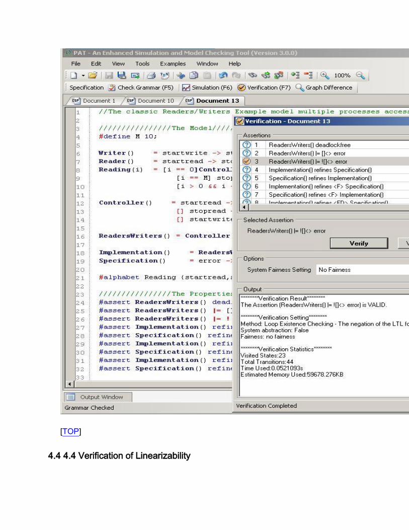
[TOP]
4.4 4.4 Verification of Linearizability

Linearizability is an important correctness criterion for implementations of objects
shared by concurrent processes, where each process performs a sequence of
operations on the shared objects. Informally, a shared object is linearizable if each
operation on the object can be understood as occurring instantaneously at some point,
called the linearization point, between its invocation and its response, and its behavior
at that point is consistent with the specification for the corresponding sequential
execution of the operation. One common strategy for proving linearizability of an
implementation (used in manual proofs or automatic verification) is to determine
linearization points in the implementation of all operations and then show that these
operations are executed atomically at the linearization points. However, for many
concurrent algorithms, it is difficult or even impossible to statically determine all
linearization points. Especially, it is extremely hard and trivial for this to be the
users' responsibility to specify such a linearization points.
While in our work, we proposed a new method- which is already integrated in PAT,
for automatically checking linearizability based on refinement relations from abstract
specifications to concrete implementations. There is no need for you to have any
knowledge on specifying linearization points. And if you can give out such information,
PAT can definitely take advantage of them to be much faster and more precise. Our
method is complete and sound with carefully manual proving, as well as efficient due
to optimization methods and the sufficient experiments. For more information please
refer to our paper [LIUWLS09].
As to linearizability as refinement relation, we should first look into an operation of a
process on a shared object. In general, such an operation has three major actions: the
invocation action of object, the linearization action(compute based on the sequential
specification of the object) and the response action, we will have a clear example in the
following part. These actions can be view as high level actions compared with the
concept of low level actions such as when reading a certain variable, the low level
action is to find the certain position pf the variable, while the high level actions only
cares about such read and response action. Thus we will have a refined specification to

the detailed implemention of model, which only has the major sequence of events which
will potentially contain a linearization point.
Above, we have explored a bunch of ideas including linearizability, linearization point
and linearizability as refinement relation. Instead of keeping telling massive concepts,
we will explore an simple example named K-valued single-writer single-reader
register (PAT examples-> Linearizability Examples-> the first one) to see be aware of
these ideas.
The implementation of this algorithm is modeled as follows:
Readers() = read_inv -> UpScan(0);
UpScan(i) = if(B[i] == 1) { DownScan(i - 1, i) } else { UpScan(i + 1) };
DownScan(i, v) =
if(i >= 0) {
if(B[i] == 1) { DownScan(i - 1, i) } else { DownScan(i - 1, v) }
} else {
read_res.v -> Readers()
};
Writer(i) = write_inv.i -> tau{B[i] = 1;} -> WriterDownScan(i-1);
WriterDownScan(i) = if(i >= 0) { tau{B[i] = 0;} -> WriterDownScan(i-1) } else
{ write_res -> Skip };
Writers() = (Writer(0)[]Writer(1)[]Writer(2)); Writers();
Register() = Readers() ||| Writers();
Note: The Reader process first does a upward scan from element 0 to the first non-
zero element i, and then does a downward scan from element i -1 to element 0 and
returns the index of last element whose value is 1. Event read_res.v returns this index
as the return value of the read operation. The Write(v) process first sets the v-th
element of B to 1, and then does a downward scan to set all elements before i to 0.
Note that in this implementation, the linearization point for Reader is the last point where

the parameter v in DownScan process is assigned in the execution. Therefore, the
linearization point can not be statically determined. Instead, it can be in either UpScan
or DownScan.
The abstract mode will be like the following with low-level actions hided:
ReadersAbs() = read_inv -> tau{M=R;} -> read_res.M -> ReadersAbs();
WriterAbs(i) = write_inv.i -> tau{R=i;} -> write_res -> Skip;
WritersAbs() = (WriterAbs(0)[]WriterAbs(1)[]WriterAbs(2)); WritersAbs();
RegisterAbs() = ReadersAbs() ||| WritersAbs();
Note: The ReaderA process repeatedly reads the value of register R and stores the
value in local variable M. Event read_res.M returns the value in M. WriteA(v) writes the
given value v into R. Event write_inv.v stores the value v to be written into the register.
The WriterA process repeatedly writes a value in the range of 0 to K -1. External
choices are used here to enumerate all possible values. RegisterA interleaves the
reader and writer processes and hides the read and write events (linearization actions).
The only visible events are the invocation and response of the read and write
operations. This model generates all the possible linearizable traces.
Thus, we can going to check the refinement relations between the detailed model
and the abstract model to verify the linearizability of K-valued single-writer single-reader
register algorithm.

[TOP]
4.5 4.5 Timed Zenoness Checking
Because RTS module supports process constructs like deadline, it suffers from zeno
executions, i.e., infinitely many steps taking within finite time. Zeno executions are
unrealistic and therefore must be ruled out in model checking. It is known that zone
graphs are not fine enough to distinguish zeno executions. We show that the zone

graph produced by dynamic zone abstraction can be modified so that the properties are
verified with the assumption of non-Zenoness.
To remove zeno executions, PAT implements zeno checking for LTL and deadlock
assertions. Users only need to tick the "Apply Zeno Check" in the model checking form.
[TOP]
5. 5 Developer Guild
As model checking is emerging as an effective software validation method that it is
always desirable to have a dedicated model checker for domain specific applications.
While considering the development work that highly relies on both domain and model
checking knowledge, it is quite difficult and nontrivial to build a dedicated model
checker.
Whereas in our PAT framework, we have this layered design and modularized
feature that allows our tool to be easily extended! The so-called intermediate
representation layer (IRL) which separates modeling from verification, enables the
underlying model checking algorithms (or other analysis techniques like testing) to be
shared by different modules. For more details, please refer to section 5.1 PAT
Architecture.
[TOP]
5.1 5.1 PAT Architecture
In our PAT framework, we adopt a layered design with an intermediate
representation layer (IRL), which separates modeling languages from model checking
algorithms. Hence these algorithms (or other analysis techniques like testing) can be
shared by different languages. As shown in the figure below, PAT's architecture has
four layers, which split the model checking process into three steps:

compilation,abstraction and verification. This separation reduces the coupling between
different functionalities, hence increases the reusability of lower layers and the
extensibility of upper layers. The four layers are introduced in the following:
Modeling Layer
Modeling layer contains modules of the supported application domains (e.g.,
distributed system, service oriented computing, security protocols and so on). It
identifies the domain specific language syntax, well-formness rules as well as formal
operational semantics, which are all encapsulated in a separate module. Two key
components which are the language parser and model components (including syntax
classes, variables, channels, etc.) consists this layer.
Abstraction Layer
Since model checking techniques only work with finite state systems, while a system
often has infinitely many states according to its concrete operational semantics, that
(automated) state abstraction is essential. In this layer, we applied abstraction
technique into systems. For instance, zone abstraction abstract infinite TTSs into finite
ones, process counter abstraction to group identical processes using process counter
variables and ignore process identifiers (if they are irreverent) which reduces state
space significantly. Partial order reduction to reduce all possible interleave execution
orders of parallel running processes into a particular execution order is another effective
method.
Intermediate Representation Layer (IRL)
After compilation and abstraction, the input model is converted to some form of
internal representations, which is the basis of the model checking algorithms.
Intermediate representation layer contains different semantic representations for
different model checking approaches.
For explicit model checking, three configuration interfaces are defined, i.e., LTS-
the most general semantic models for untimed systems, TTS- the common
semantic model for Timed Automata and timed process algebras, and MDP- for

probabilistic systems. Each of the interfaces has a number of operations, which
allow the underlying model checking algorithms (such as methods:
MoveOneStep and GetID) to drive the execution of the system and collect
information from system states. The configuration interface can also be used by
the simulator to show the system state space graphically.
For symbolic model checking, different operations are defined capture the
language semantics, e.g., in the form of Boolean formulae. The Boolean
formulae are usually stored in the form of Binary Decision Diagram (BDD) for
symbolic model checking or Conjunctive Normal Form (CNF) for bounded model
checking. For BDD-based symbolic model checking, a method EncodeProcess is
defined for each language construct.
Analysis Layer (IRL)
This layer contains reusable model checking algorithms. For each intermediate
representation in IRL, a set of algorithms are developed. For example, deadlock
checking, reachability checking, LTL verification with or without fairness assumptions,
refinement checking have been developed for LTS. If the verification result is false, a
counterexample is produced, which can be visualized via simulator.

[TOP]
5.2 5.2 PAT Class Diagram
Model checking involves functions like state-space exploration, process scheduling
enumeration, and state management. In the actual implementation of existing model
checkers, these functions are highly tangled in order to achieve optimal performance.
PAT is designed to allow reusing and extending the functions. We choose C# as the
implementation language for the benefits of Object-Oriented design and competitive
performance. By applying DESIGN PATTERNs [GAMMAHJV95], the implementation
details are successfully hided with proper encapsulation. The coupling between the
components is reduced and then extensibility can be achieved. We further apply this

design strategy to module interface design. The dependency between common library
and individual modules is minimized.
PAT's design is hierarchical, as reflected in the class diagram in the following figure.
The system consists of two basic packages, namely PAT.GUI and PAT.Common, and
11 module packages. Each of the 11 modules implements necessary module interfaces
and is packed into a plug-in DLL. The complete API can be found in section 5.4 PAT
APIs.
We use the CSP module as a demonstrating example to explain the implementation
details which involves implementation of GUI package & Common Package and Module
Package in section 5.2.1 and 5.2.2 respectively.
[TOP]
5.2.1 5.2.1 GUI and Common Package

PAT.GUI package
This package implements main graphical user interfaces and the plug-in
architecture. GUI package loads the syntax files of different modules during the system
initialization, which stores the syntax information (e.g., keywords, folding, and auto-
completion) and module information. When users want to perform syntax checking,
simulation or verification of an input model, the linked module is loaded into the system
dynamically using reflection technique and then the corresponding interface method is
invoked.
PAT.Common package
As shown in the Class Digram prevously, PAT.Common package consists of three
parts which are module interfaces, common GUI and shared libraries.
Module Interfaces
The module interface adopts ABSTRACT FACTORY pattern, where
ModuleFacadeBase is the abstract factory, and ModuleFacade classes in each
module are concrete factories. The product is Specification interface, and the
concrete products are the actual Specification implementations in modules. The
clients of using the products are the GUI classes. This pattern separates the
details of different modules from their general usage.
Abstract class ModuleFacadeBase in PAT.Common package defines the
module interface. It behaves as the central gate communicating with the
GUI package by adopting the FACADE design pattern, i.e., check the
syntax, show simulator window and model checker window. Note: All
modules must implement this interface in order to be recognized by the
plug-in framework.
Specification is the interface class for the internal representation of system
models. It also uses FACADE pattern to communicate with SimulatorGUI
and ModelCheckerGUI which are the common GUIs, to provide the

information of the user input model. Specification is composed by system
model and properties (named Assertions in the class diagram) which are
to be verified. Since system model information is module dependent,
Specification is only associated with Assertions in the common package.
Shared Library
The Expression and Value classes define the interfaces for a simple but
general WHILE language with variables and some primitive values. Though
these classes should be implemented in the actual module, we move them to the
common library so that they can be shared by all modules. Variable values need
to be cloned if one state has more than two outgoing transitions. To
systematically implement the clone process for all values, we adopt the
PROTOTYPE pattern for Value class and its subclasses, where the Clone
method creates new objects by copying the existing ones.
Besides the module interfaces and shared library, PAT.Common package contains
the intermediate layer and verification algorithms in the analysis layer.
The LTSState Class
Since we take CSP module for the running example, the intermediate
representation layer here is just one abstract class LTSState, which implements
a single transition with a target state in LTS definition. The transition's label is
stored in the Label property, and target state information (e.g., variable valuation,
channel buffer, program counter and so on) shall be realized in the actual module
since it is module related. MoveOneStep method generates all the possible
transitions starting from the target state. GetID method returns the unique
hashed string representation of the label and target state. The two abstract
methods shall be realized in the actual modules and will be used by the
verification algorithms. It is clear that starting from an initial state, these methods
are sufficient to generate the complete state space.
Note: If symbolic model checking is used, the EncodeProcess abstract

method should be realized in actual module to encode the target state and
outgoing transitions to Boolean formulae that can be used by the symbolic model
checker or SAT solvers.
The Assertion Class
Assertion class defines the interface for properties. It has one initial state,
from where it explores the system state space and produces a counterexample if
the property is not satisfied. Because verification algorithms need to keep track of
visited states or have a scheduler if the concurrent processes have different
priorities, a StateManager and a SchedulingManager are linked with the
Assertion for verification algorithm to use them to store the states and perform
process scheduling without worrying about the actual implementation. These two
classes also adopt the STRATEGY pattern since a number of state hashing and
scheduling strategies are possible.
Currently, for LTS verification, four categories of assertions are supported as
shown in Class Diagram. For example, for safety properties (e.g.,
DeadlockAssertion, RefinementAssertion and ReachabilityAssertion), three
searching strategies are possible: depth-first-search (DFS), breadth-first-search
(BFS) and symbolic verification algorithm using greatest fixed point method. For
liveness properties (i.e., LTLAssertion), two searching strategies are possible:
nested DFS [GJH97] or Tarjan's strongly-connected components searching
algorithm [Tarjan72]. These strategies are selected according to users' choice
during the run-time.
Note: To increase the reusability of the code, we create the generic version of
popular algorithms using TEMPLATE pattern. For example, DFS and BFS are
searching algorithms used in all safety property verification.
To have a reusable implementation, we create a generic DFS (BFS)
algorithm with an abstract early termination condition. Different algorithms implement
the early termination condition differently. For instance, DeadlockAssertion's early
termination condition is that the current state is a deadlock state.

ReachabilityAssertion's early termination condition is that the current state satisfies the
desired condition.
[TOP]
5.2.2 5.2.2 Module Package
Each module package should first implement the module interface and specification
interface, and then the modeling layer's components, i.e., language parser (e.g.,
CSPParser), variable valuation and channel buffer (stored in Valuation) and language
syntax classes.
language syntax classes
The language syntax classes in CSP module naturally form a COMPOSITE pattern
by following the language grammar. Each language construct (e.g., parallel
composition, sequential compositions, choice process and so on) is implemented as a
single class, which implements the Process interface with two key methods:
MoveOneStep and EncodeProcess. These two methods implement the semantics of
the language syntax for the two different model checking approaches. MoveOneStep
method follows the operational semantic rules to realize the state transitions from
current state to a list of target states. EncodeProcess performs the encoding of the
syntax to Boolean formulae that can be used by the symbolic model checker or SAT
solvers.
CSPState class
The most important class to be implemented is the CSPState class, which realizes
the concrete transitions of the LTS. For CSP#, each system state contains the current
valuation of variables, buffered elements in the channels and current active process.
This composition is exactly implemented in the Class Diagram. The MoveOneStep
method (or EncodeState method) in CSPState class will invoke the MoveOneStep (or
EncodeProcess) method of the current active process by providing current variable

valuation and channel buffer data. This guarantees that LTS is generated by following
the operational semantics. At this point, modeling layer is completed.
Abstraction and Reduction Techniques
Most of the abstraction and reduction techniques are highly language dependent.
For example, different timed related operators in real-time systems shall update the
zones in different ways. Partial order reduction strategies require information about
processes, global variables, dependencies of transitions, control-flow of processes, etc.
This restriction makes the abstraction layer hardly fully independent from modeling
layer. Most of the abstraction and reduction techniques are embedded inside method
MoveOneStep or EncodeState to produce a reduced state space. In PAT, we
demonstrate these techniques by code samples and libraries so that our experiences
can be reused.
[TOP]
5.3 5.3 PAT Extensions
In this section, we discuss the possible extensions of PAT with the help of the pre-
defined APIs, examples and libraries. These extensions allow domain experts to create
customized model checkers in all levels, based on their knowledge of the model
checking.
Basically, we will introduce how to create a dedicated model checker by means of
following four ways which will be covered in detail in four sub-sections respectively.
Language Translation: Translating models into a language supported by an
existing module in PAT through the module APIs.
Language Extension: Extending one of the existing languages with new syntax,
data types or libraries.
Algorithm Extension: Extending PAT with general or domain specific new model
checking algorithms, state reduction techniques or abstraction techniques.

Module Extension: Extending PAT with a completely new module supporting a
new language.
After reading over all the four methods, you will be skilled to develop your own
model checker. Have fun!
[TOP]
5.3.1 5.3.1 Language Translation
The easiest way of creating a model checker is to create a syntax rewriter from a
domain specific language to an existing language in PAT. This is only recommended if
the domain language is less expressiveness than the existing languages.
Comparing with other tools, programming a language translator is straightforward in
PAT. Because PAT has well-defined APIs for Specification facade class and module
language constructs, users only need to create the Specification model and generate
the language constructs objects using these APIs. For example, Specification class in
CSP# module offers the interfaces to create global Variables, Channels, Processes and
Assertions. This approach requires little interaction with PAT codes. Most importantly,
the target language model is automatic generated from the Specification class, which
can guarantee syntax correctness. The usefulness of this extension has been
demonstrated by the build-in translator from Promela4 to CSP# [ZHAO10] and the
translator from UML state diagram to CSP# [ZHANGL10].
However, sometimes this approach will be infeasible. For example, the translation
may not be optimal if special domain specific language features are present. In addition,
reflecting analysis results (e.g., showing the counterexample trace) back to the domain
model is often non-trivial.
[TOP]
5.3.2 5.3.2 Language Extension

To create a new model checker which only need to enrich a existing modeling
language, may use the following ways. You can create new data types and support new
libraries or extend the language syntax by implementing certain classes and interfaces.
Extensible Data Type and Library
For simplicity, existing modules in PAT only support integer variables, Boolean
variables and (multi-directional) arrays of integer or Boolean. However, sometimes user
defined data type is necessary and can simplify the model substantially. In the Common
project, PAT defines the interface for variable valuations, which includes methods for
hashing (or encoding) the value for state representation, a to-string method for simulator
display and deep-clone method for duplicating the values. PAT provides the
functionality to create arbitrary data type by simply creating a C# class inheriting the
Value interface. These classes can be imported into the model (based on the reflection
mechanism in .NET) and used as normal variables. We demonstrate the idea by
creating a Set data type using the code in the following Listing.
1 public class Set:HashSet < int >, Value {
2 public override string ExpressionID {
3 get {
4 String id = " " ;
5 foreach ( int element in set ) {
6 id += element + " , " ;
7 }
8 return id.TrimEnd ( ' , ' ) ;
9 }
10 }
11 public override string ToString( ) {
12 return " { " + ExpressionID + " } " ;
13 }
14 public override Value GetClone( ) {

15 return new Set ( this ) ;
16 }
17 public bool IsDisjoint( Set set ) {
18 foreach ( int i in this ) {
19 foreach ( int j in set ) {
20 if ( i == j ) {
21 return false ;
22 }
23 }
24 }
25 return true ;
26 }
27 }
First, Set class implements the Value interface in order to be used in PAT.
ExpressionID property returns the unique string representation of the data type at any
time. ToString method produces the pretty print of the set elements, which can be used
in the simulator. GetClone method implements the PROTOTYPE design pattern. To
implement the operations of a set, Set class inherits the generic HashSet class in
the .NET framework. Therefore existing methods in HashSet like Add, Remove are
inherited automatically. New methods can also be created easily, for example IsDisjoint
method. Compared with Bogor's set extension, our approach is much simpler. To use
the Set class, users only need to import the compiled DLL and declare the variable of
Set type. The variable can be initialized using new keyword and methods of Set class
can be invoked as in traditional OO program. The syntax of using the user defined data
type can be found in section 2.5 Using C# Code as Libraries.
Another benefit of the extensible data type design is that users can control the data
hashing function, which may reduce the state space significantly. For example, a check
board can be presented by the position of pieces only without including the empties

spaces. Therefore, the ExpressionID property can be defined to contain only positions
of pieces to speedup the verification.
Language Syntax Extension
In general, the input language of a model checker must be carefully designed, with
preciseness, intuitiveness and efficiency in mind. A minor syntax extension or
modification may require re-examination of the whole system. PAT facilitates such
extensions with the following design supports.
All the parsers in PAT are developed using ANTLR parser generator with clearly
documented grammars rules. New language syntax can be easily added by
changing the grammar rules and generating the code automatically.
Each language syntax is implemented in a single class (refer to PAT.CSP
package in the class diagram), which implements its semantics. To support new
language syntax, only one class needs to be implemented by following the
syntax class interface (e.g., the Process class in the class diagram). PAT's
layered design requires minimum change in the system and all model checking
algorithm developed can be reused.
Taking the probabilistic module PCSP as an example, it extends the concurrent
system modling language CSP# with one additional language feature, i.e., probabilistic
choices. Knowledge about existing modules is required and a new parser is created for
the extended language features.
[TOP]
5.3.3 5.3.3 Algorithm Extension
It is possible that a domain may have specialized properties and require dedicated
model checking algorithms for these properties. For abstraction techniques, they are
highly language dependent and hard to extend. These two cases usually need special
care as we will elaborate them in detail respectively in the following two parts.

Property Extension
PAT's design allows seamless integration of new model checking algorithms and
optimization techniques. To create a new property, users need to create a new
assertion class, inheriting the base Assertion class and implementing its methods. The
dedicated model checking algorithm is implemented in the Verify method. In addition,
method GetCounterExample must be implemented if a concrete counterexample is to
be generated.
Note: that GetCounterExample is optional for some modules. For instance, for
probabilistic model checking based on MDP, the verification result is a probability range,
e.g., with more than 0.5 and less than 0.85 probability a property is satisfied, which may
not require the generation of a counterexample.
PAT offers a number of algorithm templates like generic DFS and BFS algorithm to
help the development of model checking algorithms. Furthermore, supporting functions,
like LTL to Büchi or Rabin or Streett automata conversion which is essential for LTL
model checking, or DBM library which is for real-time system verification, are provided
in PAT. With the help of PAT's design, we have successfully extended PAT with the
algorithms for divergence checking, timed refinement checking in real-time system
module and new deadlock and probabilistic reachability checking recently.
Abstraction Extension
In general, abstraction techniques are to be encoded as part of language semantics,
in the MoveOneStep or EncodeProcess methods of each language construct in each
module. PAT offers a framework for abstract-refinement techniques. If over-
approximation abstraction is applied, users must override the method to check whether
a generated counterexample is spurious or not and override the method to re ne the
abstraction.
Currently, PAT offers one module independent abstraction, i.e., process counter
abstraction. Parameterized systems are characterized by the presence of a large (or

even unbounded) number of behaviorally similar processes, and they often appear in
distributed/ concurrent systems. A common state space abstraction for checking
parameterized systems groups behaviorally similar processes rather than keeping track
of all process identifiers. When a system with identical concurrent processes, process
counter abstraction can be implemented by invoking the library provided in PAT to
update the counter and mark the group of identical processes as abstracted. The
verification algorithms will automatically recognize this mark and check the generated
counterexample is spurious due to the abstraction or real counterexample. With the
provided sample code, process counter abstraction can be implemented quickly and
correctly.
[TOP]
5.3.4 5.3.4 Module Extension
Module extension is the last resort if the previous approaches are not applicable. In
this case, users need to write a parser according to the language syntax, implement the
language construct classes to encode the operational semantics of each and every
language construct, and lastly, make connections with the intermediate layer. (Please
refer tp a recently developed tool Module Generator can help you to create your module
easily. )
This approach is the most complicated compared with ones discussed previously.
Nevertheless, this approach gives the most flexibility and efficiency. It is difficult to
quantify the effort required to build a high-quality module in PAT. Experiences suggest
that a new module can be developed in months or even weeks in our team. This
approach is still feasible for domain experts who have only the basic knowledge on
model checking, since model checking algorithms and state space reduction techniques
are separated from modeling languages. In order to make use of the model checking
library, only knowledge on the module interfaces and IRL is necessary.

To illustrate the feasibility of this approach, we elaborate the process of creating the
TA module to support verification of Timed Automata models. The graphic interface for
drawing Timed Automata is based on an existing module (e.g., the LTS module which
allows users to draw LTSs). We omit the details here. Besides, creating this TA module
involves 4 steps.
1. Create a package for the module and add the PAT.Common package in
package's references (In the actual implementation, a package will be a C#
project of type "Class Library". The output of the project is a single DLL file.
PAT.Common package is a DLL, which can be found in PAT's installation folder).
2. Implement the module interfaces so that the module can be recognized by PAT.
Module interfaces include two classes, i.e., ModuleFacade and Specification,
which are the same as the CSP module shown in the class diagram.
3. Create a parser and the language related classes. The input language of TA
module is a network of timed automata running in parallel. For each automaton,
there are a set of states and transitions between the states. Because this
modeling language is not hierarchical as CSP# (hence no need to apply
COMPOSITE pattern), only one language syntax class is needed for the TA
network and one class to store a single automaton. The global variables and
channels can be implemented in the same way as CSP# module using Valuation
class (refer to the Class Diagram). Clock variables and valuations can be
implemented using Difference Bounded Matrix package provided by
PAT.Common package. The expressions (variable assignments, guard
conditions, etc.) can reuse the classes inside common package.
4. Connect with the intermediate layer by implementing the TAState. In TA module,
each TAState should include the Valuation of global variables and channels,
clock zones of type DBM and a TA network.
In total, users only need to implement 7 classes to create a module, i.e., 2 interface
classes, 1 parser class, 3 language related components and 1 state interface. With the

basic understanding of model checking and PAT tool design, we finish the TA module
within a month.
[TOP]
5.3.5 5.3.5 Using PAT as Library
In this part, we shall look at the process of using PAT as a library in details. As PAT
is written in C#, for simplicity, we only discuss the steps of referencing PAT library in
C#.
1 Preliminary Settings
To link up to the PAT library, several references have to be added into the project
first. "PAT.Common" is an essential package that must be added in. The .dll file
"PAT.Common.dll" is located at the root folder of your PAT installation. Then depending
on the modules to be used, the corresponding references also need to be added. For
example, if the CSP module is to be used, then "PAT.Module.CSP" should be included
into the reference list. The .dll files can be found at "Modules" folder under the root.
Note that the "Modules" folder itself also needs to be copied to the execution directory.
If user defined C# library is to be imported to the model, then the .dll files of the library
should be put under "Lib" folder of the execution directory.
2 Sample Codes
Below are some sample codes of how to use provided methods in the PAT library to
run model verifications.
1. Load the module base of a specific module and parse the model specification
using the loaded module base.
o using PAT.Common;
o using PAT.Common.Ultility;

o using OutOfMemoryException =
PAT.Common.Classes.Expressions.ExpressionClass.OutOfMemoryExcep
tion;
o using PAT.Common.Classes.Assertion;
o using PAT.Common.Classes.Expressions.ExpressionClass;
o using PAT.Common.Classes.LTS;
o using PAT.Common.Classes.Ultility;
o
o //Load the module
o modulebase = PAT.Common.Ultility.Ultility.LoadModule("CSP");
o
o //Parse the model specification
o SpecificationBase Spec =
modulebase.ParseSpecification(ModelSpecification, "", "");
o
2. After parsing, all the assertions in the model specification will be stored in the
"SpecificationBase". The assertions can be retrieved by looking up in the generic
library "SpecificationBase.AssertionDatabase". For instance, the following code
will get the first assertion base from the assertion database.
o AssertionBase assertion = Spec.AssertionDatabase.Values.ElementAt(0);
o
3. For each assertion, a series of settings can be applied before the verification.
The settings include all the options that can be found in the GUI version, such as,
fairness type, verbose, parallel verification, shortest witness trace, etc. Then call
the method "InternalStart()" of "AssertionBase" to start the verification.
o //Apply verification settings
o assertion.UIInitialize(null, FairnessType.NO_FAIRNESS, false, false,
false, true, false, false);
o
o //Start the verification

o assertion.InternalStart();
o
4. After the verification is done, the results will be stored in
"AssertionBase.VerificationOutput". The results include "VerificationResult" which
indicates whether the assertion is valid or not, "CounterExampleTrace" which
keeps the witness trace of the counter example found,
"EstimateMemoryUse" ,"VerificationTime", etc.
o If
(assertion.VerificationOutput.VerificationResult.Equals(VerificationResultT
ype.INVALID))
o {
//The assertion is invalid
o }
o
o //Get the counterexample trace
o string result = "";
o foreach (ConfigurationBase step in
assertion.VerificationOutput.CounterExampleTrace)
o {
result += step.GetDisplayEvent());
o }
o
5. The "OutofMemoryException" should be caught in your code.
o //RuntimeExceptions
o catch (RuntimeException ex)
o {
System.Console.Out.WriteLine("Runtime exception occurred: " +
ex.Message);
//Out of memory Exception
if (ex is OutOfMemoryException)

{
System.Console.Out.WriteLine("Model is too big, out of
memory.");
}
else
{
System.Console.Out.WriteLine("Check your input model for
the possiblity of errors.");
}
o }
o //General Exceptions
o catch (Exception ex)
o {
System.Console.Out.WriteLine("Error occurred: " + ex.Message);
o }
This section was contributed by Mr. Li Yi ([email protected])
[TOP]
5.4 5.4 Module Generator
Module Generator is to help developers to quickly build a new model checker for any
modeling language as a module of PAT. By providing module name, language syntax
construct names and choices of assertions, Module Generator automatically generates
the module project (in C#) with interface classes (e.g. ModuleFacade, Specification,
state interface etc.), language classes with code skeletons. With the generated code,
developers only need to create a parser of the new modeling language and implement
the operational semantics by completing the specific methods within the code skeletons.
A new module can be developed independently without the source code of PAT.
This approach is also feasible for domain experts who have only the basic knowledge

on model checking, since model checking algorithms and state space reduction
techniques are separated from modeling languages. Users can find this function under
the Tools tab in PAT's editor, as shown in the following figure.
In this section, you can learn (1) in Section 5.4.1 how to use Module Generator to
generate a C# project for a new model checker, (2) in Section 5.4.2 how to work with
the generated code to complete the development of the target model checker, and (3) in
Section 5.4.3 an example of developing a model checker for a simple language.

[TOP]
5.4.1 5.4.1 Module Generation
The GUI of Module Generator is shown in the following Figure.
First of all, you need to provide a module name. Module Code shall be defined as an
abbreviation of your module name. For Syantax Panel, you have to fill in the language

constructs of your new module, such as in CSP we support process interleave, parallel
etc. The module generator will create these classes automatically for you.
As for Semantics panel here, we currently support three semantic models, e.g., LTS
for CSP languages, TTS for timed systems and MDP for probabilistic systems. These
are the three intermediate representations supported in PAT. After choosing the
semantic model, the generator will automatically generate corresponding classes.
There are also a bunch of assertion checking algorithms supported and can be
reused in the new module. Code will automatically generated according to the semantic
model. You are also free to add domain specific assertions to your new module reusing
these generated algorithms.
Note: if there is any error happened, try to regenerate the code again, since the code
generation engine ( from Microsoft) is not stable sometimes.
The following table summarizes the fields of the GUI to specify before generating
codel.
Field
Type Optional Field Name Meaning Remark Example
Text box
No Module Name Name Name of the module Event
Grammar
No Module Code Module
Identifier
It will be used as the extention of
the input file of the generated
module.
EG
Yes Syntax Language
Construct
The generated code will contain
a C# class for
each language construct specified
here.
Event,
Process,
Sentence,
Sequence
Dropdown
list
Choose
one
Semantic
Model LTS
Labeled
Transition
The generated module will first
produce chosen semantic models
Labeled
Transition

from the
three
System and then execute corresponding
model check algorithms on the
semantic model.
System
( LTS)
TTS
Timed
Transition
System
MDP
Markov
Decision
Processes
Check
box NA
Generated
BDD Encoding
Methods
As
named.
Tick this check box and the BDD
encoding methods will be
generated automatically, allowing
developers to use PAT's BDD
library for optimizing verification.
NA
Supported
Assertions
Deadlockfree
The interface of the deadlock
checking algorithm will be
generated.
Reachability
Checking
The interface of the state-
reachability checking algorithm
will be generated.
Linear
Temporal Logic
The interface of the LTL
checking algorithm will be
generated.
Deterministic
Checking
The interface of the deterministic
checking algorithm will be
generated.
Divergence
Checking
The interface of the Divergence
checking algorithm will be
generated.
Refinement
Checking
The interface of the refinement
checking algorithm will be

generated.
[TOP]
5.4.2 5.4.2 Working with Generated Code
The generated code is a complete C# solution with two projects: PAT.Main and
PAT.Module."Your Module Code". To work with the code, open "PAT3 Source.sln"
using Visual Studio 2008 or later. The code structure is displayed below.
Note: the code should be compilable. If not, please try to re-generate the code.
PAT.Main is the GUI project which contains a simple editor which allows developers
to input a model for simulation and verification. You don't need to modify this project for
your module development.
PAT.Module."Your Module Code" is the module project. The classes inside this
project are explained below. Or you can refer to Section 5.2.2 for more details.

Assertions folder contains all the assertions to be supported. Unless you want to
develop your own assertions, otherwise you don't need to change anything.
LTS folder contains all the syntax classes, specification class and state interface
class. Sample LTS syntax classes can be found in the subfolder for your reference. You
need to develop a parser and put inside this folder. Specification class is the internal
representation of the input model. Configuration class is the state interface.
ConfigurationWithChannelData class is the state interface used for synchronous
channel communication. If you module doesn't have synchronous channel, then there is
no need to have this class.
Ultility folder contains some ultility functions.
ModuleFacade class is the module interface class to communicate with GUI classes.
You only need to change this class if you want to add some examples for your module.
The code templates are inside this class for you to follow.
Note: if there is any question of using the generated code, please email
[TOP]
5.4.3 5.4.3 Example
In the following, we will show how to use PAT Module Generator to generate a new
model checker:
(A). Generate Code with Module Generator
(B). Complete the generated code
(C). Executing and testing the new model checker
The source code of this example can be downloaded here.

A modle language Simplified CSP (SCSP), which is a small subset of CSP, is used
as a running example for the purpose of illustration. In SCSP, a process is constructed
only by event prefixing or interleaving. The syntax of SCSP is as follows:
P = e -> P | P ||| P | Skip;
(A). Generate Code with Module Generator
With the Module Generator, it is very convenient and simple to generate the code for
a SCSP model checker as illustrated by the following figure.

Once the code generation is completed, the following dialogue will appear to inform
you.
Now you can open the Windows Explorer to locate the generated C# project:
(B). Complete the generated code
Double click PAT3 Source.sln and you will open the C# solution in Microsoft Visual
Studio.

In the generated solution, there are two projects:
PAT.Main, contains the interface to the GUI package of PAT; one can refine the
GUI editor for the language by re-implementing the class EditorTabItem.cs, and
re-organizing error messages by modifying ErrorListWindow.cs.
Note: no modification is required here, unless one want to re-implement the
editor.
PAT.Module.SCSP, contains the code for all the rest stuffs, as follows:

o Assertions: this folder provides model checking for deadlock and state
reachability checking, recalling that in part ( A) only these two kinds of
assertions are chosen to be supported. Thus, the parser should support
the syntax for these two types of assertions, too. In the generated code,
the default model checking algorithms of PAT are inherited, and
developers can re-implement the algorithms by him/herself.
o LTS: this folder contains two catergories of functionality. The first is to
provide a parser to analyze a SCSP model, and the second is to describe
each language construct as a class and integrate the semantics of each
language construct into the method MoveOneStep.
Note that the parser classes are not generated automatically. Thus, one
needs to create parser classes manually, e.g., SCSPTreeLexer.cs,
SCSPTreeParser.cs, and SCSPTreeWalker.cs.
Besides, there are two classes that are created for specific purposes.
Configuration.cs, the class the represents the semantic model
of your language. By default, the code is complete and you need
not modify anything.
Specification.cs, the controlling class, which communicates
with ModuleFascade.cs and LTS. Two methods are important and
should be completed in order to make the code effects, and they
are:

1. ParseSpec(): code should be added here to invoke the
parser to analyze the input model. Note that this method will
be invoked before each request of simulation or verification.
Meanwhile, also make sure that each assertion has been
initialized within this method, by code like the following:
2. SimulationInitialization(): code should be added here to
generate the model list (at least one model) that will appear
in the simulator window, once simulation button is clicked.
Note that if this method is not implemented, the simulatior
would not function properly.
The rest of classes in LTS are all language construct representations,
including Definition, DefinitionRef, EventPrefix, Interleave, Process, Skip
and Stop. Make sure that proper instances are created by the parser
based on a certain input model.
(C). Executing and testing the new model checker

Editing a SCSP model in the editor:
Simulating it:

Verifying it:


[TOP]
6. 6 FAQs
The FQAs are divided to two subsections:
Installation FAQ
Using PAT FAQ
[TOP]
6.1 Installation FAQ
Q1: I can not install PAT!
Answer:
1) Make sure you have installed the .NET framework 4.0.
2) Make sure the installation file is correctedly downloaded:
"PAT3.Setup.XXX.msi". Some users accidentally rename the installation file with
extra .exe in the end.
3) The last remedy is to download direct executable of PAT and run it directly
without installation.
Q2: Can I run PAT in linux or Solaris, Mac OS X and Unix?
Answer: Yes. See section 2.1 for the details.
Q3: Cannot start PAT 3.exe on mono
Answer: If the error message informs that assembly System.Windows.Forms is
missing, please get the packages libmono-winforms1.0-cil and libmono-winforms2.0-cil.

If you get "Could not get XIM" error, one way you could do is to set the environment
variable as "export MONO_WINFORMS_XIM_STYLE=disabled".
Q4: I can not start the simulator for old version of PAT!
Answer: Please make sure you have System.Core.dll under PAT installation folder.
[TOP]
6.2 Using PAT FAQ
Q1: How to debug in PAT?
Answer:
PAT does not provide runtime debugger. Nevertheless, you can easily do the
debugging using variable range checking, assertions or simulator.
1) Explicitly providing the range for the global variables, e.g., var x{1..120};. if the
variable's range is out of bound in simulation or verification, PAT will throw
runtime exception as the feedback.
2) Using assert(condition) process inside your program. Assert(condition) will
throw a PAT runtime exception during the execution if the condition is evaluated
to be false.
3) Writing simple (safety) assertions on global data to check whether they are
violated or not, e.g., #assert system |= [] invariant; where invariant can be the
desired property you want to guarantee.
4) If your model is small, you can quickly using simulator to trace the behaviors of
your model or generate the complete state space.
Q2: How do I know that my model is error-free?
Answer:

After finishing your model, you can check the syntax of your model by clicking Check
Grammar button. If your model is syntactically correct, PAT will display the parsed
model in the output window in the bottom. You can check the parsed model to confirm
that your model is the one you want. Note: sometimes, a missing bracket or simple typo
can produce a different model.
All module parsers in PAT support error recovery, e.g., they can automatically add
missing brackets or remove extra brackets or semi-colons. However, all error recovery
information will be displayed as warnings in Error List window (see the Figure below).
You need to be careful if there are warnings after parsing, because the error recovery
feature may parse the model to a different one than you want. We suggest you to clear
out all warnings before doing any analysis.
Q3: When I run the model, PAT crashes like following. What should I do?
Answer:

PAT tries to catch all the exceptions internally. However, if the model gives a stack
overflow exception, then PAT cannot catch it. The reason of stack overflow exception is
most likely because your model has self-loop like following example. Be careful when
using ifa with looping back.
var x = 0;
P = ifa(x==1) {Skip} else{P};
Q4: Is it possible to imprt new Lib file in local folder?
Answer:
Yes. The complied .dll file can either be inside the Lib folder of the installation folder
or the under the same directory with the model file.
Q5: For the following program, can the two processes P() and Q() synchronise on
the event a? Then how to make them synchronise on 'a' and preserve the execution of
statement block ({x++}) in an atomic fashion?
var x=0;
P() = a{x++} -> b -> P();
Q() = a -> c -> P();
System() = P() || Q();
Answer:
A intuitive solution is to put the event 'a' and increment statement in a 'atomic' action
as follows:
P() = atomic{a -> update{x++} -> Skip};b -> Skip;
Q() = a -> c -> Skip;
aSystem() = P() || Q();
Then x will be updated right after a is engaged, and a will be synchronised.

The other possible solution could be:
P() = a -> update{x++} -> a1 -> b -> P();
Q() = a -> a1 -> c -> P();
[TOP]
7. 7 References
[Tarjan72] R. Tarjan. Depth-first Search and Linear Graph Algorithms. SIAM Journal
on Computing, 2:146.160, 1972.
[WangPD94] Wang Yi, Paul Pettersson and Mats Daniels.Automatic Verification of
Real-Time Communicating Systems by Constraint Solving. In Proceedings of the 7th
International Conference on Formal Description Techniques, pages 223-238, North-
Holland. 1994.
[Mat09] The MathWorks. Stateflow and Stateflow Coder User's Guide, March 2009.
[SCAIFESCTM04] N. Scaife, C. Sofronis, P. Caspi, S. Tripakis, and F. Maraninchi,
Defining and translating a safe- subset of Simulink/Stateflow into Lustre, EMSOFT 2004
ACM, pp. 259-268.
[HAMON&RUSHBY07] G. Hamon and J. M. Rushby, An operational semantics for
Stateflow, International Journal on Software Tools for Technology Transfer, 9(5-6): 447-
456, 2007.
[UMLGuide] G. Booch, J. Rumbaugh and I. Jacobson, The Unified Modeling
Language User Guide SECOND EDITION, Addison Wesley Professional, 2005.
[HOARE85] C.A. Hoare. Communicating Sequential Processes. Prentice-Hall
International, Englewood Cliffs, New Jersey, 1985.

[GAMMAHJV95]E. Gamma, R. Helm, R. E. Johnson, and J. Vlissides.
DesignPatterns: Elements of Reusable Object-Oriented Software. Addison-Wesley,
1995.
[HUTH&Ryan04]. Micheal Huth and Mark Ryan. Logic in Computer Science. ?SPAN
class=GramE>Cambridge University Press 2004.
[ROSCOE97] A.W. Roscoe. The Theory and Practice of Concurrency. Prentice-Hall,
1997.
[LIUSD08b] Y. Liu, J. Sun and J. S. Dong: An Analyzer for Extended Compositional
Process Algebras. ICSE Companion 2008: 919-920. Bib
[AWR97] A. W. Roscoe. The Theory and Practice of Concurrency. Prentice-Hall,
1997.
[GJH97] G. J. Holzmann. The Model Checker SPIN. IEEE Transactions on Software
Engineering, 23(5):279?95, 1997.
[SUNLDP09] J. Sun, Y. Liu, J. S. Dong and J. Pang: Towards Flexible Verification
under Fairness. CAV 2009.
[LIUSD10] Yang Liu, Jun Sun and Jin Song Dong: Analyzing Hierarchical Complex
Real-time Systems. FSE 2010.
[LIUPSZ09] Y. Liu, J. Pang, J. Sun and J. H. Zhao. Verification of Population Ring
Protocols in PAT. TASE 2009.
[SUNLDC09] J. Sun, Y. Liu, J. S. Dong and C. Q. Chen. Integrating Specification
and Programs for System Modeling and Verification. TASE 2009.
[ZHANGLSDCL09] S. J. Zhang, Y. Liu, J. Sun, J. S. Dong, W. Chen and Y. A. Liu.
Formal Verification of Scalable NonZero Indicators. SEKE 2009.

[LIUWLS09] Y. Liu, W. Chen, Y. A. Liu and J. Sun. Model Checking Linearizability
via Refinement. FM 09.
[SUNLRLD09] J. Sun, Y. Liu, A. Roychoudhury, S. S. Liu and J. S. Dong. Fair
Model Checking with Process Counter Abstraction. FM 09.
[SUNLDZ09] J. Sun, Y. Liu, J. S. Dong and X. Zhang. Verifying Stateful Timed CSP
using Implicit Clocks and Zone Abstraction. ICFEM 09.
[LIUSD09] Y. Liu, J. Sun and J. S. Dong. Scalable Multi-Core Model Checking
Fairness Enhanced Systems. ICFEM 09.
[ZHAO10] W. Zhao. Yet Another Model Checker for PROMELA - theTransformation
Approach. In MoCSeRS 2010, pages 131?32. IEEE Computer Society, 2010.
[ZHANGL10] S. Zhang and Y. Liu. An Automatic Approach to Model Checking UML
State Machines. In SSIRI 2010, pages 131?32. IEEE Computer Society, 2010.
[ORCUserGuide] http://orc.csres.utexas.edu/userguide/pdf/all.pdf.
[AQDKJM09] A. Q. David Kitchin and J. Misra. Quicksort: Combining concurrency,
recursion, and mutable data structures. Technical report, The University of Texas at
Austin, Department of Computer Sciences."
[MAJM10] M. AlTurki and J. Meseguer. Dist-Orc: A Rewriting-based Distributed
Implementation of Orc with Formal Analysis. Technical report,
https://www.ideals.illinois.edu/handle/2142/15414.
[TOP]


