
Probing the reheating phase through
primordial magnetic field and CMB( based on arXiv:2012.10859v2 [hep-th] )
Md Riajul Haque
Department of Physics,
IIT Guwahati, Assam, India

2
❑ Motivation
❑ Inflationary Magnetogenesis
❑ Connecting Reheating and Primordial magnetic field via CMB
❑ Numerical Results
❑ Main points and outcomes

3
Motivation
▪ Why reheating phase is import?
• Indirect bound on reheating dynamics ( Taking into account
both the CMB and present value of the magnetic field)

4
❑ We Address :
❖ In the current study we consider present day Large Scale Magnetic Field (LSMF) and
CMB anisotropy to probe the reheating phase of the universe followed by the standard
inflationary phase.
❖ Conventionally after the end of inflation, the magnetic field on the super-horizon scales
redshifts with the scale factor as provided inflaton energy density transfers into
plasma and the universe become good conductor instantly right after the end of inflation.
❖ In the reference Kobayashi et al. Phys. Rev. D 100, no.2, 023524 (2019) it has been
shown that if the conductivity remains small redshifts of magnetic energy density becomes
slower, , due to electromagnetic Faraday induction. This helps one to obtain
the required value of the present-day large scale magnetic field.
❖ Taking into account both the CMB anisotropic constraints on the inflationary power
spectrum, and the present value of the the large-scale magnetic field, our analysis reveals
an important connection among the reheating parameters , magnetogensis models
and inflationary scalar spectral index.

5
Inflationary Magnetogenesis
❑ Electromagnetic power spectrum :
❖ FLRW metric background expressed in conformal coordinate:
❖ The gauge field action:
❖ In order to quantize the field components are in terms of irreducible scalar and vector
components .
❖ One write in terms of annihilation and creation operator:
❖ The equation of motion of the mode function:
❖ Conventionally the electromagnetic power spectrum is expressed in terms of those mode
functions:

6
❖ In order to diagonalize the Hamiltonian, we employ the Bogoliubov transformation
❖ and are the Bogoliubov coefficients defined as :
❖ The power spectrum in terms of Bogoliubov coefficients :
❑ Modelling the coupling function
❖ We consider the widely considered power-law form of the coupling function
❖ The solution of the mode function considering perfect de-sitter background Hubble
parameter :
7
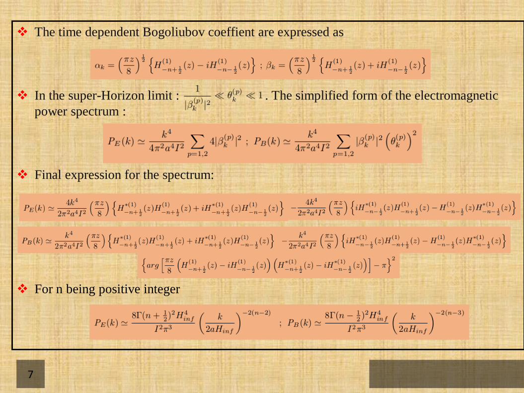
❖ The time dependent Bogoliubov coeffient are expressed as
❖ In the super-Horizon limit : . The simplified form of the electromagnetic
power spectrum :
❖ Final expression for the spectrum:
❖ For n being positive integer
8
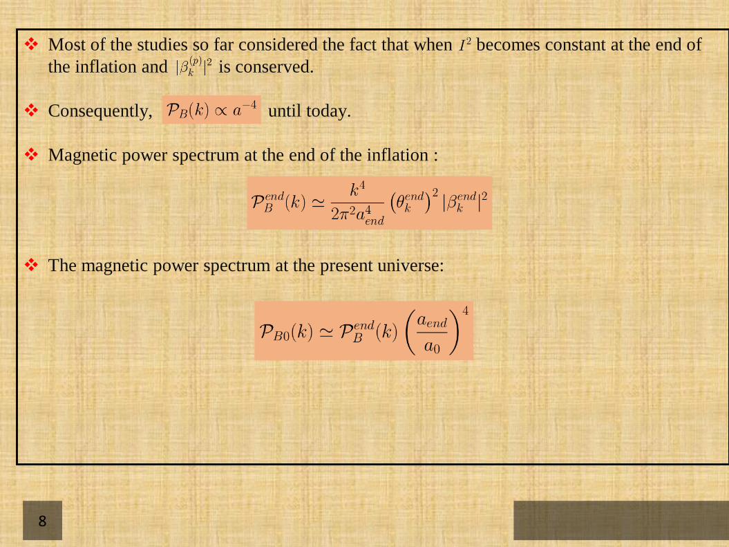
❖ Most of the studies so far considered the fact that when becomes constant at the end of
the inflation and is conserved.
❖ Consequently, until today.
❖ Magnetic power spectrum at the end of the inflation :
❖ The magnetic power spectrum at the present universe:

9
❖ It is clear that the required magnetic field strength G is difficult to achieve
within the conventional framework, unless one introduces slow decreasing rate of
magnetic energy density in some early state of universe evolution.
10
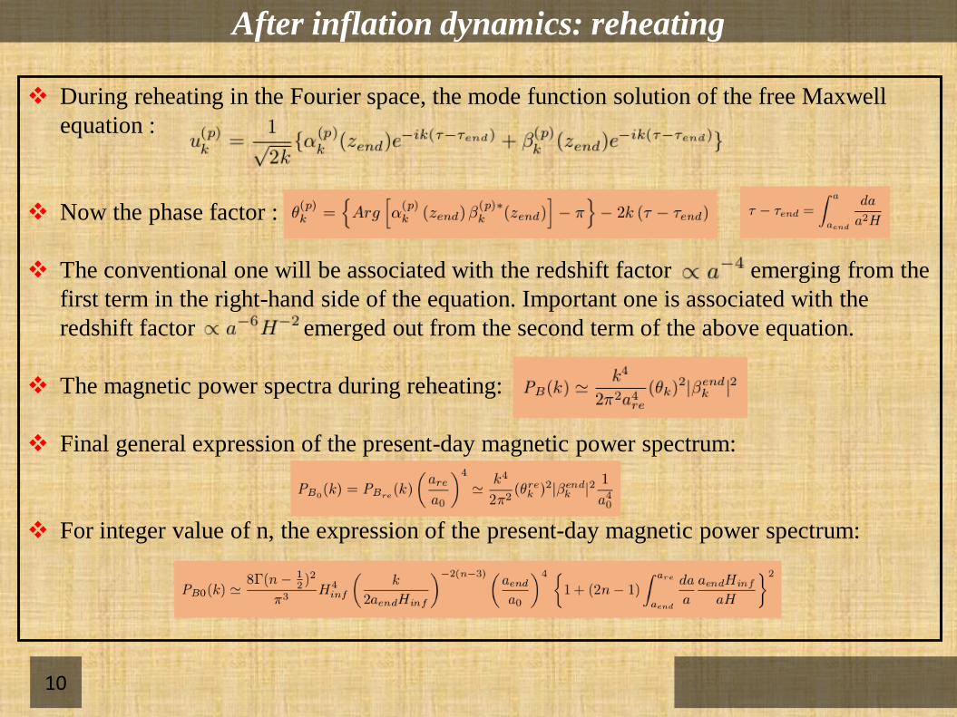
After inflation dynamics: reheating
❖ During reheating in the Fourier space, the mode function solution of the free Maxwell
equation :
❖ Now the phase factor :
❖ The conventional one will be associated with the redshift factor emerging from the
first term in the right-hand side of the equation. Important one is associated with the
redshift factor emerged out from the second term of the above equation.
❖ The magnetic power spectra during reheating:
❖ Final general expression of the present-day magnetic power spectrum:
❖ For integer value of n, the expression of the present-day magnetic power spectrum:
11
Reheating dynamics: Connecting Reheating and Primordial
magnetic field via CMB
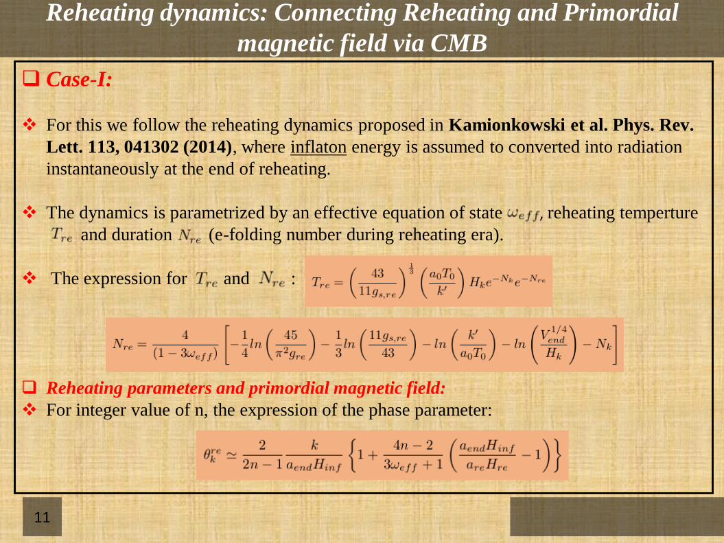
❑ Case-I:
❖ For this we follow the reheating dynamics proposed in Kamionkowski et al. Phys. Rev.
Lett. 113, 041302 (2014), where inflaton energy is assumed to converted into radiation
instantaneously at the end of reheating.
❖ The dynamics is parametrized by an effective equation of state , reheating temperture
and duration (e-folding number during reheating era).
❖ The expression for and :
❑ Reheating parameters and primordial magnetic field:
❖ For integer value of n, the expression of the phase parameter:
12
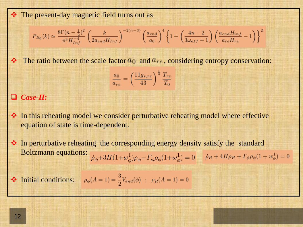
❖ The present-day magnetic field turns out as
❖ The ratio between the scale factor and , considering entropy conservation:
❑ Case-II:
❖ In this reheating model we consider perturbative reheating model where effective
equation of state is time-dependent.
❖ In perturbative reheating the corresponding energy density satisfy the standard
Boltzmann equations:
❖ Initial conditions:
13
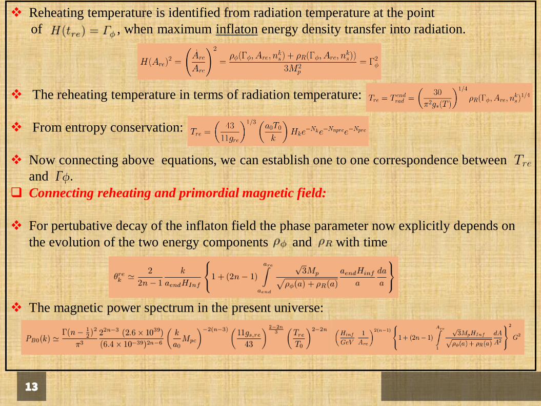
❖ Reheating temperature is identified from radiation temperature at the point
of , when maximum inflaton energy density transfer into radiation.
❖ The reheating temperature in terms of radiation temperature:
❖ From entropy conservation:
❖ Now connecting above equations, we can establish one to one correspondence between
and Γϕ.❑ Connecting reheating and primordial magnetic field:
❖ For pertubative decay of the inflaton field the phase parameter now explicitly depends on
the evolution of the two energy components and with time
❖ The magnetic power spectrum in the present universe:

14
Discussion on strong coupling and backreaction problem
❖ As coupling function monomial function of scale factor , for negative value of n
the gauge kinetic function increasing during inflation.
❖ The coupling function boils down to unity after inflation. The effective electromagnetic
coupling, for negative values of n becomes very large, which turns the
theory non-perturbative.
❖ On the other hand, if one considers positive values of , throughout the inflationary
period the gauge kinetic function will always larger than unity, so there is a
considerable reduction of the effective electromagnetic coupling . Strong coupling
problem can be avoided for positive values of n but backreaction problem arise as
production of electromagnetic energy can generically take over the background energy
density.
❖ To avoid backreaction problem:

15
❖ Total gauge field energy density at a given scale factor during inflation can be
calculated as:
❖ For example, the scale-invariant electric power spectrum which corresponds to n=2, the
total gauge field energy density at the end of the inflation
❖ However, scale-invariant magnetic power spectrum (n=3), immediate back-reaction
problem as the electric field power spectrum, for large scale limit
.
16
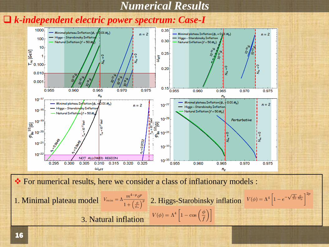
Numerical Results
❑ k-independent electric power spectrum: Case-I
❖ For numerical results, here we consider a class of inflationary models :
1. Minimal plateau model 2. Higgs-Starobinsky inflation
3. Natural inflation
17
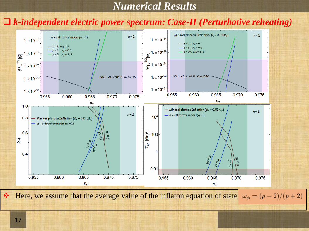
Numerical Results
❑ k-independent electric power spectrum: Case-II (Perturbative reheating)
❖ Here, we assume that the average value of the inflaton equation of state
18
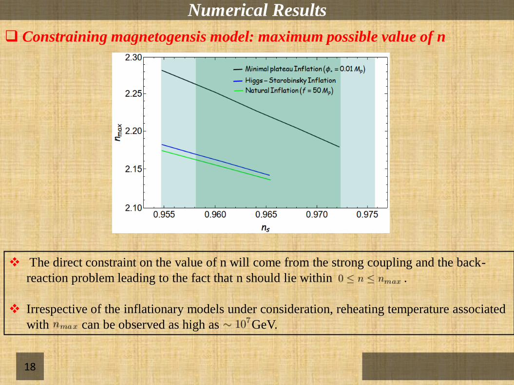
Numerical Results
❑ Constraining magnetogensis model: maximum possible value of n
❖ The direct constraint on the value of n will come from the strong coupling and the back-
reaction problem leading to the fact that n should lie within .
❖ Irrespective of the inflationary models under consideration, reheating temperature associated
with can be observed as high as GeV.

19
Main points and outcomes
❖ we can clearly predict a unique value of associated with a specific choice of the
present magnetic field. Additionally, for a given the reheating temperature is also
determined uniquely.
❖ Taking into account CMB constraints the reheating phase can be uniquely probed by the
evolution of the primordial magnetic field
❑ Scale invariant electric power spectra:
❖ For case-I reheating scenario, irrespective of models under consideration large scale
magnetic field constrains the effective equation of state within and
consequently predicts the low value of reheating temperature GeV.
❖ For the perturbative reheating scenario the range of inflaton equation of state
is found to be observationally not viable for G.
❖ This observation provides us a strong constraint on the possible form of the inflaton
potential near its minimum with considering the aforesaid observable limit of the
present-day magnetic field strength.
❑ Constraining magnetogensis model:
❖ Considering both backreaction and strong coupling problems into account, the maximum
allowed value of n would be .

20
THANK YOU


