
Principal Component Analysis
Source: Introduction to Machine Learning Computing Science 466 / 551
R. Greiner, B. Póczos, University of Alberta https://webdocs.cs.ualberta.ca/~greiner/C-466/
1 ABDBM © Ron Shamir

Contents • Motivation • PCA algorithms • Applications • PCA theory
Some of these slides are taken from • Karl Booksh Research group • Tom Mitchell • Ron Parr 2 ABDBM © Ron Shamir

3
Data Visualization Example:
• Given 53 blood and urine measurements
(features) from 65 individuals
• How can we visualize the measurements?
ABDBM © Ron Shamir

4
Data Visualization • Matrix format (65x53)
H-WBC H-RBC H-Hgb H-Hct H-MCV H-MCH H-MCHCH-MCHCA1 8.0000 4.8200 14.1000 41.0000 85.0000 29.0000 34.0000 A2 7.3000 5.0200 14.7000 43.0000 86.0000 29.0000 34.0000 A3 4.3000 4.4800 14.1000 41.0000 91.0000 32.0000 35.0000 A4 7.5000 4.4700 14.9000 45.0000 101.0000 33.0000 33.0000 A5 7.3000 5.5200 15.4000 46.0000 84.0000 28.0000 33.0000 A6 6.9000 4.8600 16.0000 47.0000 97.0000 33.0000 34.0000 A7 7.8000 4.6800 14.7000 43.0000 92.0000 31.0000 34.0000 A8 8.6000 4.8200 15.8000 42.0000 88.0000 33.0000 37.0000 A9 5.1000 4.7100 14.0000 43.0000 92.0000 30.0000 32.0000
Inst
ance
s
Features
Difficult to see the correlations between the features... ABDBM © Ron Shamir

5
Data Visualization • Spectral format (65 pictures, one for each person)
0 10 20 30 40 50 600100200300400500600700800900
1000
measurement
Value
Measurement
Difficult to compare the different patients... ABDBM © Ron Shamir

6
Data Visualization
0 10 20 30 40 50 60 7000.20.40.60.811.21.41.61.8
Person
H-Band
s• Spectral format (53 pictures, one for each feature)
Difficult to see the correlations between the features... ABDBM © Ron Shamir

7
0 50 150 250 350 45050100150200250300350400450500550
C-Triglycerides
C-L
DH
0 100200300400500
0200
4006000
1
2
3
4
C-TriglyceridesC-LDH
M-E
PI
Bi-variate Tri-variate
Data Visualization
How can we visualize the other variables??? … difficult to see in 4 or higher dimensional spaces... ABDBM © Ron Shamir
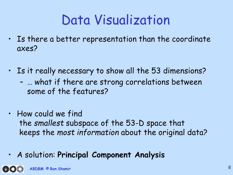
Data Visualization • Is there a better representation than the coordinate
axes?
• Is it really necessary to show all the 53 dimensions? – … what if there are strong correlations between
some of the features?
• How could we find the smallest subspace of the 53-D space that keeps the most information about the original data?
• A solution: Principal Component Analysis 8 ABDBM © Ron Shamir
9
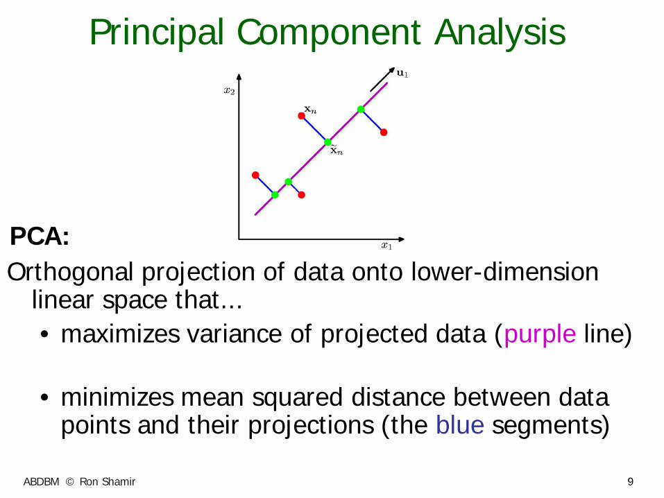
Principal Component Analysis
Orthogonal projection of data onto lower-dimension linear space that... • maximizes variance of projected data (purple line)
• minimizes mean squared distance between data
points and their projections (the blue segments)
PCA:
ABDBM © Ron Shamir
10
PCA: the idea
• Given data points in a d-dimensional space, project into lower dimensional space while preserving as much information as possible • Eg, find best planar approximation to 3D data • Eg, find best 12-D approximation to 104-D data
• In particular, choose projection that
minimizes squared error in reconstructing original data
ABDBM © Ron Shamir
11
• Vectors originating from the center of mass
• Principal component #1 points in the direction of the largest variance.
• Each subsequent principal component… • is orthogonal to the previous ones, and • points in the directions of the largest
variance of the residual subspace
The Principal Components
ABDBM © Ron Shamir

12
2D Gaussian dataset
ABDBM © Ron Shamir

13
1st PCA axis
ABDBM © Ron Shamir

14
2nd PCA axis
ABDBM © Ron Shamir
15
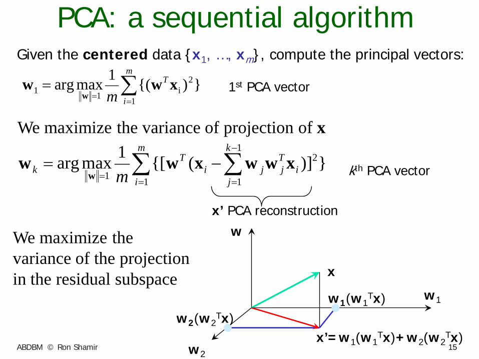
PCA: a sequential algorithm
∑ ∑=
−
==−=
m
i
k
ji
Tjji
Tk m 1
21
11})]({[1maxarg xwwxww
w
}){(1maxarg1
2i11 ∑
===
m
i
T
mxww
w
We maximize the variance of the projection in the residual subspace
We maximize the variance of projection of x
x’ PCA reconstruction
Given the centered data {x1, …, xm}, compute the principal vectors:
1st PCA vector
kth PCA vector
w1(w1Tx)
w2(w2Tx)
x w1
w2 x’=w1(w1
Tx)+w2(w2Tx)
w
ABDBM © Ron Shamir
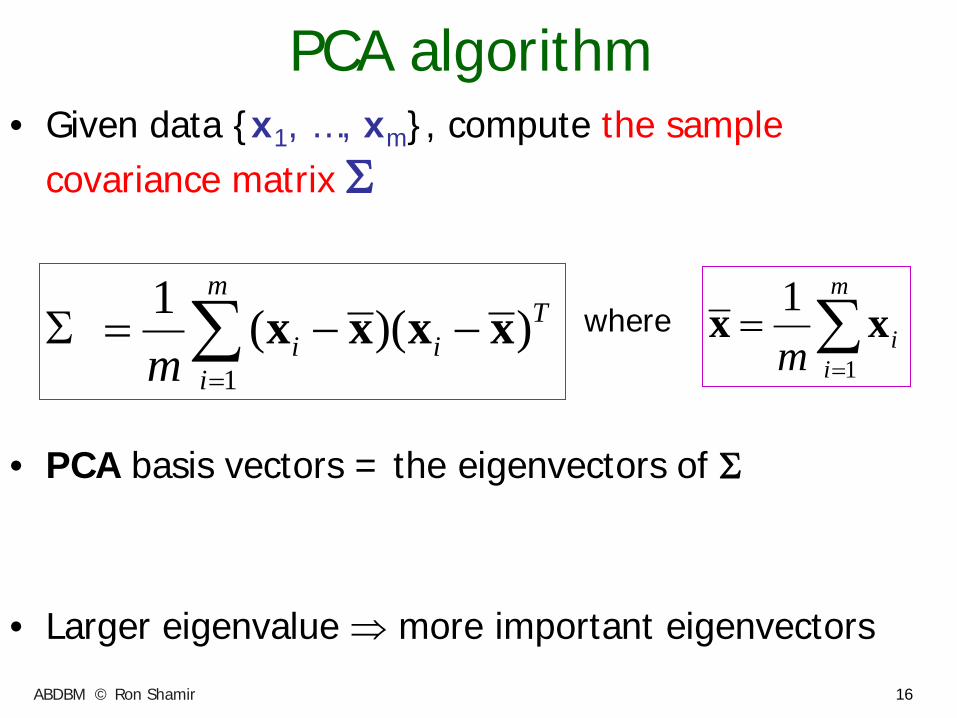
16
PCA algorithm • Given data {x1, …, xm}, compute the sample
covariance matrix Σ
• PCA basis vectors = the eigenvectors of Σ
• Larger eigenvalue ⇒ more important eigenvectors
1
1 ( )( )m
Ti i
im =
Σ = − −∑ x x x x ∑=
=m
iim 1
1 xxwhere
ABDBM © Ron Shamir

17
PCA algorithm PCA algorithm(X, k): top k eigenvalues/eigenvectors
% X = N × m data matrix, % … each data point xi = column vector, i=1..m
•
• X subtract mean x from each column vector xi in X
• Σ X XT … covariance matrix of X
• { λi, ui }i=1..N = eigenvectors/eigenvalues of Σ ... λ1 ≥ λ2 ≥ … ≥ λN
• Return { λi, ui }i=1..k % top k principal components
∑=
=m
im 1
1ixx
ABDBM © Ron Shamir
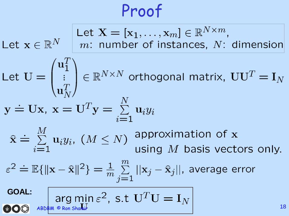
Proof
GOAL: 18 ABDBM © Ron Shamir
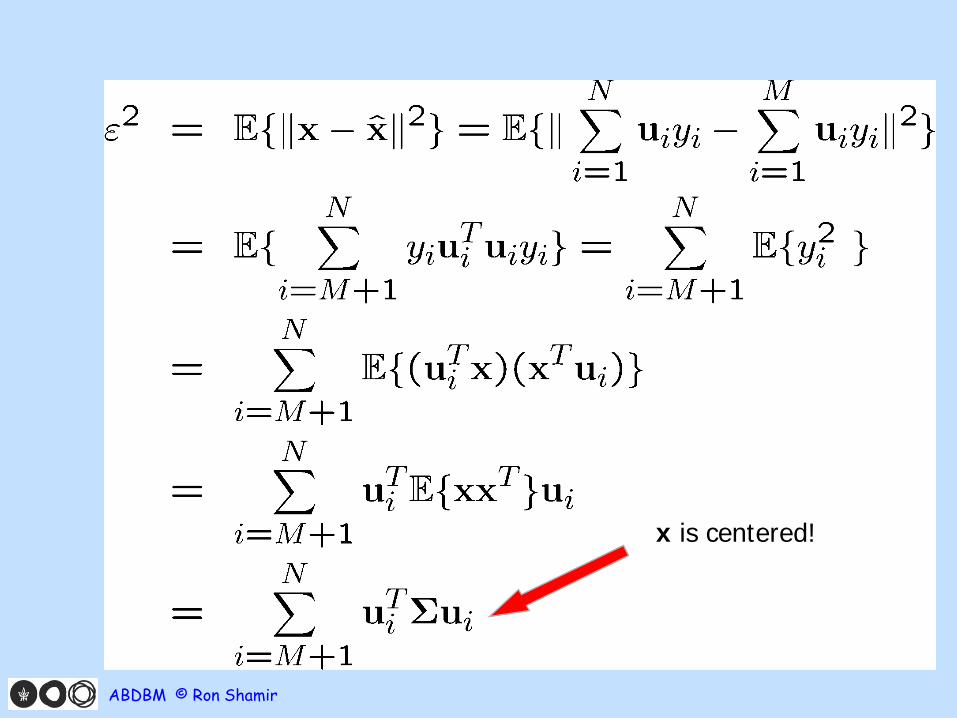
x is centered!
ABDBM © Ron Shamir

Justification of Algorithm II GOAL:
Use Lagrange-multipliers for the constraints.
ABDBM © Ron Shamir

ABDBM © Ron Shamir

22
PCA Applications • Data Visualization • Data Compression • Noise Reduction • Data Classification • … • In genomics (and in general): a first step
in data exploration: does my data have inner structure? Is it clusterable?
ABDBM © Ron Shamir
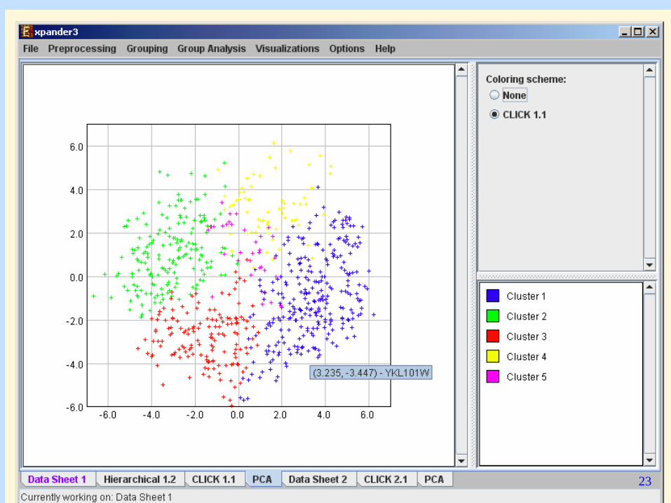
23

A PCA result of ALL 21 samples using 7,913 genes. Red: good prognosis (upper right), Blue: bad prognosis (lower left).
Nishimura et al, GIW 03 24 ABDBM © Ron Shamir

PROMO demo
ABDBM © Ron Shamir 25

26
PCA shortcomings
PCA doesn’t know labels
ABDBM © Ron Shamir

28
PCA shortcoming (3)
PCA cannot capture NON-LINEAR structure ABDBM © Ron Shamir
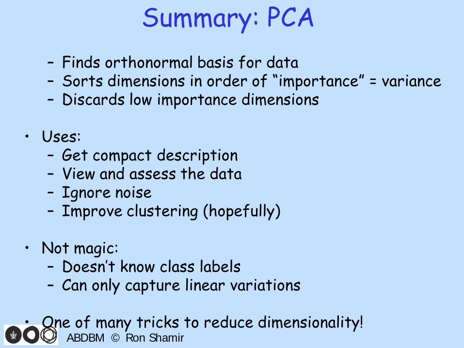
Summary: PCA – Finds orthonormal basis for data – Sorts dimensions in order of “importance” = variance – Discards low importance dimensions
• Uses:
– Get compact description – View and assess the data – Ignore noise – Improve clustering (hopefully)
• Not magic:
– Doesn’t know class labels – Can only capture linear variations
• One of many tricks to reduce dimensionality!
ABDBM © Ron Shamir

Karl Pearson, father of mathematical statistics (1857-1936)
ABDBM © Ron Shamir 30
Invented PCA in 1901. Rediscovered multiple times in many fields.


