
Power-Aware Compile Technology
Xiaoming Li

Frying Eggs

Future CPU?
intel!Micro32
Fred Pollack
8
1
10
100
1000
!"#$ !$ %"&$ %"#$ %"'#$ %"(#$ %"!)$ %"!'$ %"!$ %"%&$
Watt
s/c
m2
i386i486
Pentium ® processor
Pentium Pro ® processor
Pentium II ® processor
Pentium III ® processor
Power density continues to get worse
Surpassed hot-plate power density in 0.5$
Not too long to reach nuclear reactor
Hot plate
Nuclear Reactor
RocketNozzleSun’s
Surface
( Source: Fred Pollack, Intel, Micro 1999 keynote)
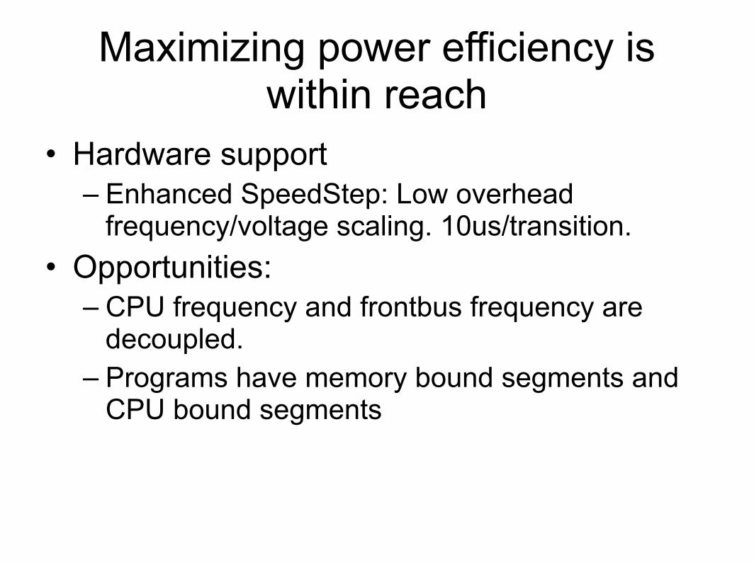
Maximizing power efficiency is within reach
• Hardware support– Enhanced SpeedStep: Low overhead
frequency/voltage scaling. 10us/transition.
• Opportunities:– CPU frequency and frontbus frequency are
decoupled. – Programs have memory bound segments and
CPU bound segments

Is any energy wasted when executing programs?
• Current Status:– Programs run at a single frequency from start to
end, neglecting segmental behavior of execution.
– CPU idles in memory bound segments.
• Out plan:– Find out how a program execute.– Remove the fat in energy consumption

Searching for the most power efficient FFT
• Select the proper frequency/voltage for different regions in the FFT code.– Challenges include:
• Where to switch?
• Which frequency?
• Schedule the code to reveal more opportunities for frequency scaling.– Challenges include:
• How to schedule for power?

What previous research does?
• Hardware/OS– [Berkeley, MIT, UMD, UMich, UVa, …]
• Interactive applications– Predict memory access pattern– Fix window size -> Wrong prediction
• Batch applications– Predict the execution time of every task– Distribute unused time to remaining tasks– Low granularity, no use for DSP program
7

Previous Compiler-based DVS algorithms
• “The Design, Implementation, and Evaluation of a Compiler Algorithm for CPU Energy Reduction” Chung-Hsing Hsu and Ulrich Kremer, PLDI 03.
• Select basic blocks from program structure
– Entry/exit is unique
– Loop– Call site– If statement– Seq. of regions– Entire procedure
8
16
L4
L3
C5
C1
C2
EXIT
ENTRY

Chung-Hsing Hsu and Ulrich Kremer’s Approach (Cont’)
• Measure the execution time and the power consumption of every region at every possible frequencies.
• Change the frequency of only one region• Exhaustive search for the best region and
the optimal frequency.
9

Run programs on the simulator
• “Compile-time Dynamic Voltage Scaling Settings: Opportunities and Limits”, Fen Xie, Margaret Martonosi, and Sharad Malik, PLDI 03
• Divide the execution into memory accesses and cpu operations.
• Assuming the processor has continuous frequency spectrum.
• Model power consumption in memory accesses phases and cpu active phases.
• Use existing optimizing software to find the best single region for scheduling.
10

Re-examine our goal
• What we really want to optimize?– Power ~ O(v)
• Trivial solution if just to reduce power
– Energy ~ O(v2)• Minimal energy consumption at the lowest frequency
– • SPEC / Jules
– • Test if we really make improvement
11
Energy ∗ Delay
Energy ! Delay2
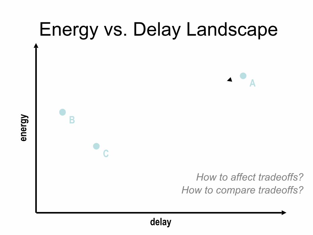
Energy vs. Delay Landscapeen
ergy
delay
B
C
A
How to affect tradeoffs?How to compare tradeoffs?

Optimization Space
delay
ener
gy
Pareto Optimal

Projection of Compile Optimizations
14
Carnegie Mellon
Project Review, November 2005, Slide J. C. Hoe, CMU/ECE
F’=(F, s, p, -O)
Joint Energy-Delay Optimizations
runtime
ener
gy
F
parallelizing scalingenerg
y-a
ware
com
pila
tion

Our Goal
15
Carnegie Mellon
Project Review, November 2005, Slide J. C. Hoe, CMU/ECE
Expanding Optimization Space
runtime
ener
gy
new, higher quality
Pareto frontfor any metric

Simulator vs. Real Machine?
• Simulator– Watt, SimPower– Power-model should be verified.– Not the best environment for compiler research.
• Real machine– How to identify phases in the program?– How to measure power consumption?– How to search the front-line of energy-delay?
16

Identify Program Phases
• Use hardware counters– Low overhead– Limited number
• Find the correct events– Memory access: L2_Cache_Load_In,
L2_Prefetch_Load_In– Instruction number: Instruction_Retired– Execution time: Cycle
17

Insert Reading Points
• Control the overhead of reading.– Reading evenly during the execution– Use a simplified model of memory accesses
and working cycles.
• Understand how compiler translate instructions.– Constant loading– Array access
18

Are there really program phases?
19
0
5
10
15
20
25
30
35
40
45
50
0 500000 1e+06 1.5e+06 2e+06 2.5e+06 3e+06
L2 C
ache M
iss/1
0 u
s
Cycle
PM

20
0
5
10
15
20
25
30
0 200000 400000 600000 800000 1e+06 1.2e+06 1.4e+06 1.6e+06
L2 C
ache M
iss/1
0 u
s
Cycle
PM

Iterations have different patterns
21

Frequency Scaling
• Select the program region with the highest cache miss ratio.– Lower the processor frequency before entering
the region.– Restore the frequency after exiting the region.
22
23
Carnegie Mellon
Project Review, November 2005, Slide 2J. C. Hoe, CMU/ECE
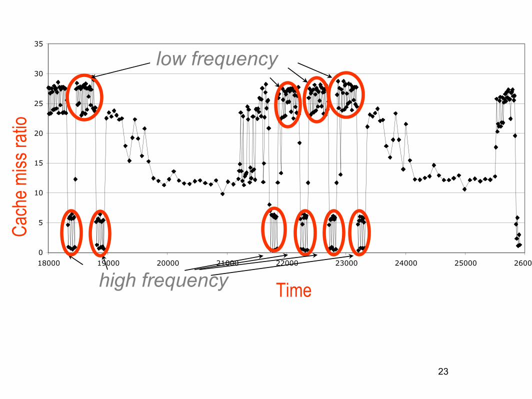
Dynamic Voltage scaling: memory profile
Ca
ch
e m
iss r
atio
Each point shows the cache miss ratio every 100 !seconds
WHT-219 (out-of-cache)
Time
0
5
10
15
20
25
30
35
18000 19000 20000 21000 22000 23000 24000 25000 26000
low frequency
high frequency

24
Carnegie Mellon
Project Review, November 2005, Slide 4J. C. Hoe, CMU/ECE
Example: code with voltage/frequency scaling instructions
setfreq(2);
i14 = 0;
while (i14 <= 32767)
{
s277 = T2[i14];
s278 = T2[32768 + i14];
t459 = s277 - s278;
…
i14++;
}
setfreq(3);
decrease frequency
increase frequency

Frequency Scaling
• Select the program region with the highest cache miss ratio.– Lower the processor frequency before entering
the region.– Restore the frequency after exiting the region.
• Transform the program to reveal more opportunities for frequency scaling.
25

26
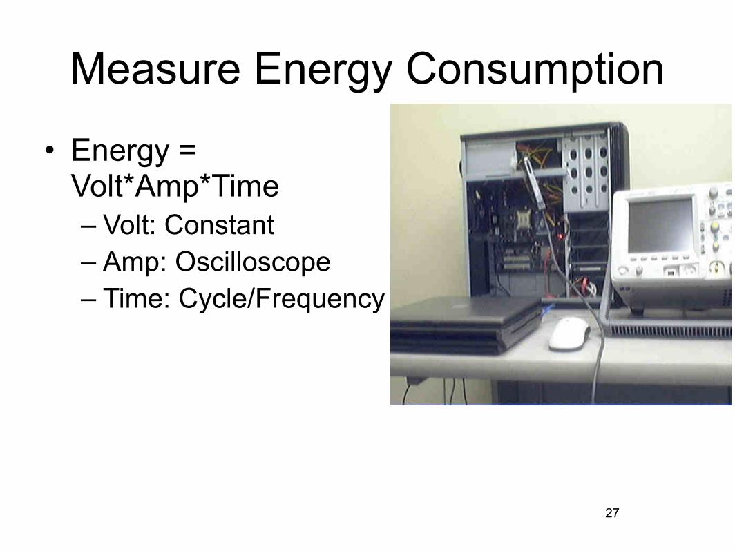
Measure Energy Consumption
• Energy = Volt*Amp*Time– Volt: Constant– Amp: Oscilloscope– Time: Cycle/Frequency
27

Pentium-M 2.13GHz
• Six frequency settings– 2.13 GHz at 1.340 volt (max performance)– 800 MHz at 0.988 volt (min performance/energy)
The change in performance/energy tradeoff is dramatic.
28

29

30

Experiment Results
31
Carnegie Mellon
Project Review, November 2005, Slide 7J. C. Hoe, CMU/ECE
0
0.2
0.4
0.6
0.8
1
1.2
0.04 0.05 0.06 0.07 0.08 0.09 0.1
Dynamic Voltage scalingE
nerg
y (J
oule
s)
WHT-220
Execution Time (Seconds)
Energy versus execution time
0
0.2
0.4
0.6
0.8
1
1.2
1.4
0.04 0.06 0.08 0.1 0.12
Fixed Dynamic
Execution Time (Seconds)E
nerg
y (J
oule
s)
Pareto curve
Withing 5% of the execution
time of the fastest version
6% energy reduction
10% energy reduction

32
Carnegie Mellon
Project Review, November 2005, Slide 8J. C. Hoe, CMU/ECE
Dynamic Voltage scalingE
nerg
y (J
oule
s)
DCT-220
Execution Time (Seconds)
Energy versus execution time
Fixed Dynamic
Execution Time (Seconds)E
nerg
y (J
oule
s)
Pareto curve
0
0.5
1
1.5
2
2.5
0.08 0.1 0.12 0.14 0.16 0.18 0.2
0
0.5
1
1.5
2
2.5
0.08 0.1 0.12 0.14 0.16 0.18 0.2

33
Carnegie Mellon
Project Review, November 2005, Slide 9J. C. Hoe, CMU/ECE
Dynamic Voltage scalingE
nerg
y (J
oule
s)
Real DFT-220
Execution Time (Seconds)
Energy versus execution time
Fixed Dynamic
Execution Time (Seconds)E
nerg
y (J
oule
s)
Pareto curve
0
0.5
1
1.5
2
2.5
0.1 0.12 0.14 0.16 0.18 0.20
0.5
1
1.5
2
2.5
0.1 0.12 0.14 0.16 0.18 0.2
34
Carnegie Mellon
Project Review, November 2005, Slide 10J. C. Hoe, CMU/ECE
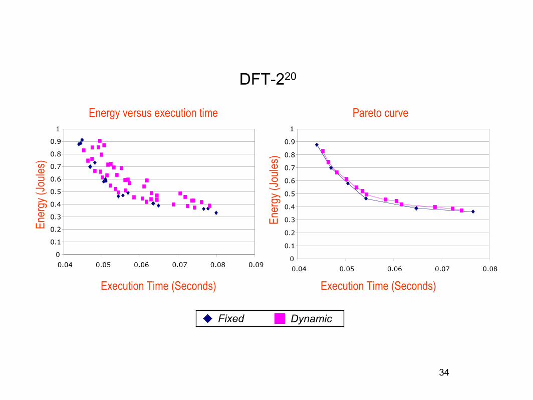
0
0.1
0.2
0.3
0.4
0.5
0.6
0.7
0.8
0.9
1
0.04 0.05 0.06 0.07 0.08 0.09
Dynamic Voltage scalingE
nerg
y (J
oule
s)
DFT-220
Execution Time (Seconds)
Energy versus execution time
Fixed Dynamic
Execution Time (Seconds)E
nerg
y (J
oule
s)
Pareto curve
0
0.1
0.2
0.3
0.4
0.5
0.6
0.7
0.8
0.9
1
0.04 0.05 0.06 0.07 0.08

Future Directions
• Loop transformation• Global optimization• Strength reduction• Parallelization for power• ...
35


