
Post-Laspeyres: The Case for a New Formula for Compiling Consumer Price Indexes
Paul Armknecht and Mick Silver
WP/12/105

© 2012 International Monetary Fund WP/12/105
IMF Working Paper
Statistics
Post-Laspeyres: The Case for a New Formula for Compiling Consumer Price Indexes
Prepared by Paul Armknecht and Mick Silver1
Authorized for distribution by Kimberly Zieschang
April 2012
Abstract
Consumer price indexes (CPIs) are compiled at the higher (weighted) level using Laspeyres-type arithmetic averages. This paper questions the suitability of such formulas and considers two counterpart alternatives that use geometric averaging, the Geometric Young and the (price-updated) Geometric Lowe. The paper provides a formal decomposition and understanding of the differences between the two. Empirical results are provided using United States CPI data. The findings lead to an advocacy of variants of a hybrid formula suggested by Lent and Dorfman (2009) that substantially reduces bias from Laspeyres-type indexes.
JEL Classification Numbers: C43, C81.
Keywords: Consumer Price Index; Index Numbers; Laspeyres, Superlative, Young, Geometric Young, Lowe index Formula.
Author’s E-Mail Addresses: [email protected] and [email protected].
1 The authors thank Walter Lane (U.S. Bureau of Labor Statistics) for his comments on an earlier draft and his assistance with the provision of data. Acknowledgements for helpful comments are also due to John Greenlees (US Bureau of Labor Statistics) and Jens Mehrhoff (Deutsche Bundesbank). The usual disclaimers apply.
This Working Paper should not be reported as representing the views of the IMF. The views expressed in this Working Paper are those of the author(s) and do not necessarily represent those of the IMF or IMF policy. Working Papers describe research in progress by the author(s) and are published to elicit comments and to further debate.

2
Contents Page
......................................................................................................................................................
I. Introduction ............................................................................................................................3
II.Higher-level price index number formulas used in practice ..................................................5 A. Arithmetic formulas ..................................................................................................5 B. Geometric counterparts .............................................................................................7 C. Available empirical work ..........................................................................................9
III. Why Geometric higher-level price index numbers differ ..................................................10 A. Geometric Young vs. Geometric Lowe ..................................................................10 B. Comparisons with a superlative price index ...........................................................12
IV. Empirical Results ...............................................................................................................15 A. The data ...................................................................................................................15 B. Results .....................................................................................................................16 C. The Geometric formulas: differences and adjustments ...........................................17
What factors underlie the difference between the two formulas? ....................17 Averages of formulas that better track superlative indexes .............................18
V. Concluding Remarks ...........................................................................................................20

3
I. INTRODUCTION
Most national statistical offices (NSOs) use in practice what they often describe as
“Laspeyres-type” index formulas for aggregating their consumer price index (CPI) at the
higher (weighted) level. These Laspeyres-type indexes include the Young and the Lowe
indexes, both of which have serious shortcomings. It is argued here that Laspeyres-type
indexes can be replaced at little cost by more suitable formulas that use the same data and
can be compiled in real time.
A Laspeyres price index can be defined as a period 0-weighted arithmetic average of price
changes between periods 0 and t. However, it takes time to compile the results of a
household expenditure survey, so in practice statistical agencies use a prior period b survey
weights to rebase a CPI that runs from the price reference period 0 (b < 0 < t). The Young
index has as its weights the preceding survey period b expenditure shares and the Lowe index
uses period b weights price-updated (and normalized) to the price reference period 0.
Laspeyres is exceptionally used in practice for compiling CPIs. 2
This paper outlines in section IIA the features of the widely used arithmetically-based Lowe
and Young formulas. Both are considered to have major shortcomings. The Lowe index is
principally used for CPI compilation in spite of theory and evidence of severe upward bias.
However, the Lowe index has the virtue, as a fixed quantity basket index, of being simple to
explain. Analytical shortcomings with the Young index include an uncertainty a priori about
the extent and nature of its deviations from Laspeyres and relatively poor axiomatic
properties.
Section IIB continues by considering the nature of and case for the geometric equivalents of
Young and Lowe indexes, that is, the Geometric Young (sometimes referred to as the Cobb-
2 Hansen (2007) notes that in the joint UNECE/ILO survey on the CPI Manual of the 47 respondents as at September 2007, 32 national statistical offices used the (price-updated) Lowe index and 15 the original (presumably survey period) Young weights. A few larger countries including Germany, Korea, and Japan use Laspeyres by retrospective revisions.

4
Douglas) and Geometric Lowe indexes. These geometrically-based indexes share the
advantage of their arithmetic counterparts of being able to be computed in real time and are
thus practical alternatives to arithmetic versions. Existing empirical work on the differences
between these formulas is outlined in section IIC.
In section III we focus on these geometric formulations. To better understand their
properties, a formal exact decomposition is derived for the difference between the Geometric
Young and Geometric Lowe indexes. However, the empirical arbiter of which is the most
suitable is their proximity to a superlative index, such as the Törnqvist index, something also
considered in this section.3
Section IV provides empirical results using CPI data from the United States. The
relationships between the Laspeyres-Paasche interval and the arithmetically-weighted Young
and Lowe indexes are considered followed by an examination of the relationship between the
Törnqvist index and the Geometric Young and Geometric-Lowe indexes. We find the
Geometric Young index, which is consistent with unitary elasticity of substitution, has a
downward bias. The US data over the period studied demonstrate inelastic substitution
(Greenlees, 2011). However, this bias can be substantially offset by averaging. The
averaging of such indexes has a formal justification from Lent and Dorfman (2009) and we
consider variants of this approach. Of note is that the Lowe price index, as used in the US
and many other countries, is found to have a bias (against superlative indexes) several times
that of some of these variants, all of which can be computed in real time using the same
database as the Lowe index.
3 The Consumer Price Index (CPI) Manual (ILO et al., 2004) recommends superlative price indexes—the Fisher, Törnqvist, and Walsh indexes—as the target formulas for the higher-level indexes. These formulas generally produce similar results, use geometric averaging, and symmetric weights based on quantity or expenditure information from both the reference and current periods. They derive their support as superlative indexes from economic theory. A utility function underlies the definition of (constant utility) cost of living index (COLIs) in economic theory. Different index number formulas can be shown to correspond with different functional forms of the utility function. Laspeyres, for example, corresponds to a highly restrictive Leontief form. The underlying functional forms for superlative indexes, including Fisher and Törnqvist, are flexible: they are second-order approximations to other (twice-differentiable) homothetic forms around the same point. It is the generality of functional forms that superlative indexes represent that allows them to accommodate substitution behavior and be desirable indexes. The Fisher price index is also recommended on axiomatic grounds and from a fixed quantity basket perspective (ILO et al., 2004).
5
Laspeyres itself has the advantage of being an upper bound to a theoretical cost-of living
index (COLI). The widely used Lowe index is likely to fall above Laspeyres. Its main
advantage is that as a fixed quantity basket index it is easy to explain; biased but easily
explained. We propose alternative formulas that can be readily computed in real time.
II. HIGHER-LEVEL PRICE INDEX NUMBER FORMULAS USED IN PRACTICE
A. Arithmetic formulas
The Laspeyres price index is given by:
0 000 0 0
0 00 0 0
0 0 0 01 1 1
1 1
, where
ti
i it tn n nt ii i i i iL i in n
i i ii i ii i i i
i i
pp q
pp q p p qI s s
p q pp q p q
(1)
The first term of equation (1) is a standard representation of the Laspeyres formula as a fixed
quantity basket index with 0ip and 0
iq denoting, respectively, prices and quantities in period 0
for i = 1,…, n products/elementary aggregates. In practice CPIs are compiled as a weighted
average of price relatives, given by the second and third terms in equation (1), where the
weights are the expenditure shares in period 0, 0.is
It takes time to compile and process household expenditure survey data, so there is a lag
between the expenditures share survey period, b, and their first use in the index, commencing
at the price reference period 0. Thus, in practice, the Laspeyres is generally not used for real
time CPI compilation and expenditure shares from the earlier period b may be used to weight
period 0 to period t price changes. The resulting Young price index is given by:
01
1
, wheret b bn
t b bi i iY i i n
b bi ii i
i
p p qI s s
p p q
(2)
More typically, weights are price-updated between period b and the price reference period 0
to effect fixed period-b quantities. The resulting Lowe index is given by:

6
00
0 01 11
00 0
1 11
t tn nnb b bi i it bi i i ib i i
i it i i iiLo n nn
b bb b ii i i ii i b
i ii i
p p pp q p qp q
p p pI
p p q p qp qp
(3)
The expression in square brackets in the first term are the period-b expenditures, b bi ip q , price-
updated to period 0. The second term shows the Lowe index to be a period-b fixed-quantity
basket price index, and the third term to be a weighted average of price changes where the
weights are hybrid period 0 prices and period b quantities, with little economic meaning.
Price-updating the expenditure shares for price changes is not to make the weights more up-
to-date, but to transform the index from a fixed period b expenditure share-weighted index of
price changes to a fixed period b quantity basket price index.
Balk and Diewert (2003), from the perspective of the economic theory of index numbers,
establish the substitution bias of a Lowe CPI—see also ILO et al., (2004, chapters 15 and 17)
and Balk (2010). Not only is the Lowe index shown to have a likely upward substitution bias
against a Laspeyres index, but the Laspeyres index has an upward substitution bias against a
superlative index. ILO et al., (2004, chapter 16) demonstrates that the Lowe index, however,
has good axiomatic properties.4
The Young index fails the circularity and time reversal tests (ILO et al., 2004, Appendix 15.3
and chapter 16). The Young index between periods 0 and t will exceed its time antithesis,
that is, its inverse between period t and 0, and in this sense is positively biased.5 ILO et al.
(2004, chapter 15) demonstrate how the discrepancy between Laspeyres and Young is
difficult to gauge. It is based on the covariance of the difference between expenditure shares
4 It passes the time reversal test and is transitive. However, as pointed out by ILO et al., (2004, paragraph 1.64), “Achieving transitivity by arbitrary holding the quantities constant, especially over a very long period of time, does not compensate for the potential biases introduced by using out-of-date quantities.”
5 It will exceed its time antithesis by a term equal to the Young index times the weighted variance of deviations of price relatives (between periods 0 and t) and their mean. Since the variance must be positive, the Young must exceed the inverse of its time antithesis except when there is no price change dispersion, a case that negates the purpose of an index number.

7
between period b and 0 and the deviations of period 0 to t relative prices from their mean.6 A
positive covariance would put Young above Laspeyres and negative covariance below
Laspeyres, possibly closer to a superlative index. Analytical shortcomings with the Young
index are thus the uncertainty a priori about the extent and nature of its deviations from
Laspeyres and its relatively poor axiomatic properties.
B. Geometric counterparts
For elementary-level indexes, the CPI Manual recommends the use of the (geometric) Jevons
index if weights are not available for individual varieties in the sample (ILO et al., 2004,
chapter 20). Using a geometric formula at the higher level would be compatible with the
currently widely used Jevons index at the lower level and would have the benefit of
maintaining consistency in aggregation.
Formulas (4) and (5) are the geometric counterparts to (2) and (3) and can be readily adopted
by statistical offices since they use the same weights and price relatives as the Young and
Lowe indexes. The Geometric Young price index is given by:
01
1
where, .i
b
t b bnt bi i iGY i n
b bi ii i
i
sp p qI s
p p q
(4)
The geometric version of the Lowe price index with its price-updated weight is given by:
0
00
001
1
where, .i
b
t bnt bi i iGLo i n
bi ii i
i
sp p qI s
p p q
(5)
The (superlative) Törnqvist index is given by:
0
01
/2t
i itnt iT
i i
pI
p
s s
(6)
6 The concern is whether the share of expenditure increases over periods 0 and b with relative price increases over periods 0 and t. This would require long-run trends in prices and, for Young to be above (below) Laspeyres, very elastic (inelastic) demand (ILO et al. (2004, chapter 15, pages 275-6).
8
for which current period expenditure shares, tis , are not available in real time. It is apparent
that for constant expenditure shares over periods 0 and t, consistent with unitary elasticity of
substitution, the Geometric Young index given by (4) equals the Törnqvist index given by
(6).
Balk (2010) demonstrates that the substitution bias of the Geometric Young index is less than
the substitution bias of the currently widely-used Lowe index. The CPI Practical Guide
supports the use of the Geometric Young formulas (UNECE et al., 2009, page 160, ff. 50). 7
The CPI Manual considers the Geometric Young index to be a serious practical possibility
for CPI compilation; since the requisite weights are available in real time, and it is less
susceptible to bias. With unitary elasticity of substitution, the Geometric Young can be
shown to lie within the Laspeyres- Paasche interval. The Geometric Young index, as its name
suggests, corresponds to cost-of-living indexes for utility-maximizing households with
Geometric Young preferences. The CPI Manual cites as its main concern the unlikelihood of
it gaining general acceptance in the foreseeable (then 2004) future since it cannot be
interpreted as a fixed quantity basket index. (ILO et al., 2004, chapter 1 paragraphs 1.40 and
9.137).
Unlike the (arithmetic) Lowe index given by (3), the Geometric Lowe (and like the
Geometric Young) indexes have no fixed quantity basket definition. The price updating of
the weights has no rationale for the Geometric Lowe. Its standing is so low that neither the
CPI Practical Guide nor the CPI Manual mentions it. However, the (arithmetic) Lowe is
widely used in practice. It is invariably described in terms of a weighted average of price
changes, albeit with little reference to such weights given in the last term of equation (3),
which have little economic meaning. There is a prima facie case for some formal and
empirical analysis of the geometric counterpart to the arithmetic Lowe.
7 It does so in a footnote: the CPI Practical Guide focused on helping implement good practice rather than as a platform for change, but the authors/editors nonetheless considered the matter sufficiently important to footnote this point. As shown later, the Geometric Young is a good proxy for superlative indexes if the elasticity of substitution is unity.
9
C. Available empirical work
Given concern about arithmetic formulations and some positive aspects of geometric ones,
we consider some of the available, albeit limited, empirical work on how close different
formulations lie to a superlative index.
Hansen (2007) using Danish CPI data for 1996 to 2003 found increases for the Young and
Lowe indices of 17.49 and 18.01 percent, respectively, compared with an increase in the
Törnqvist index of 17.08 percent.8 The Geometric Young index was below Törnqvist at
16.51 percent. The differences between Young and Lowe are not always trivial.9 The annual
inflation rate for 2004/5 and 2005/6 increased from 1.80 to 1.88 percent using Young but
decreased from 1.99 to 1.90 percent using Lowe.
Greenlees and Williams (2010), in a major study of the US CPI over December 1990 through
December 2008, found Lowe and Young increases to be quite similar, at 18.88 and 18.24
percent respectively, but the (chained) Törnqvist was much lower at 16.78 percent.10 The
Geometric Young index was closer to, and again below, the chained Törnqvist at 15.84
percent.
Pike et al. (2009, Table 10) —using New Zealand CPI data for June 2006 to June 2008 with
weights of 2003/4 and 2006/7 respectively price-updated to June 2006 and June 2008
quarters (the New Zealand CPI is quarterly) —found Lowe and Young to differ showing over
this period increases of 6.26 and 5.60 percent, respectively. These arithmetic formulations
were significantly higher than the 4.83 percent increase for the Geometric Young index
8 Cited Törnqvist indexes are approximations as the current period weights are expenditure shares over a period longer than the current month or quarter t, due to lack of expenditure data (the expenditure survey not being continuous) and inadequate sample sizes for the single month or quarter.
9 Rebasing took place in 1994 (for January 1996–December 1999), 1996 (Dec. 1999–Dec 2002), 1999 (Dec. 2002–Dec 2005), and 2003 (Dec. 2005–Dec 2006). The lag for the price-updating varies from 2 to 3.5 years over the links of the index.
10 The Lowe and Young indexes are based on the US Consumer Price Index for All Urban Consumers, or CPI-U. Its weights, as from 2002, cover a two year period and are revised every two years. For example, the weights in January 2010 are expenditures from 2007-2008 that were price-updated to December 2009. There is approximately a two-year lag from the midpoint of the survey period to the price reference period.

10
which appeared to understate the 5.73 percent increase measured by a retrospective Fisher
index.
So while Lowe and Young may generate similar results, their difference from a superlative
Törnqvist index is marked and of concern. The Geometric Young index generally falls below
(and there is some evidence that it is closer to) the superlative Törnqvist index.
Given the Geometric Young and Geometric Lowe are practical contenders for the CPI
aggregation formula, we now present a formal analysis as to why they might differ.
III. WHY GEOMETRIC HIGHER-LEVEL PRICE INDEX NUMBERS DIFFER
A. Geometric Young vs. Geometric Lowe
Following on from equation (4) we first define a Geometric Young price index as:
0
01
i
b
tnt i
GYi i
spI
p
and 0
01 1
ln lnt
GY
tn nb bii i i
i ii
Ip
s s yp
(7)
where
1
b bb i ii n
b b
i ii
p qs
p q
are period b expenditure shares and 0
lnti
ii
py
p
is the natural
logarithm of the ith price relative.
The difference between the logarithms of a Geometric Lowe and a Geometric Young price
index is given by:
0
0 01 10 0 1 1
0
1 1 11
ln ln
ln( ) ln( )
t tn n n nb b b bi i i b bi i i ib i i i i i
i it t i i i i iGLo GY n n nn
b b b bb b ii i i i ii i b
i i ii i
p p pp q p q s x y s y
p p pI I
p p q s x sp qp
(8)
where
0i
i bi
px
p . Adopting a Bortkiewicz (1923) decomposition:11
11 See Bortkiewicz (1923; 374-375) for the first application of this decomposition technique: we define
,/ / cov( , ) /u v u vuv u u v u v u v and /suv su as s-weighted terms for the decomposition.
(continued…)

11
0 0 1,
1
ln( ) ln( )b b b bi i i i
nbi i i
s s s st t iGLo GY i x y x yn
bi i
i
s x yI I y cv
s x
(9)
0
,0exp
b b bi i i
ts s sGLox y x yt
GY
Icv
I
(10)
where ,
bis
x y is the period-b weighted bis correlation coefficient between price relatives ix
and iy (that extend respectively from 0b and 0 t ); /b b bi i is s s
x xcv x is the period-b
weighted biw coefficient of variation for ,ix for which
biw
x is the standard deviation and
biwx is the b
iw -weighted mean of ,ix that is, a Laspeyres price index between periods b and 0.
First, it is apparent from (10) that ,
bis
x y dictates whether 0 tGLoI is larger (positive) or smaller
(negative) than 0 .tGYI For (weighted) price changes between periods b and 0 to be correlated
with (weighted logarithms of) price changes between periods 0 and t, there must be some
persistent uni-directional long-run price change over period b to t. A priori, a sign cannot be
unambiguously attached to this correlation coefficient.
Second, the magnitude of 0 0t tGLo GYI I is determined by
(a) The magnitude of ,
bis
x y —smaller ratios of 0 tGLoI to 0 t
GYI would be expected from
countries with longer time lags in utilizing and updating the weights, that is, longer
lags between periods b and 0 and periods 0 and t.
(b) The dispersion of price changes, bis
xcv and bis
y —it is well established in economic
theory and empirical work that dispersion in relative prices increases with increases in
Equation (10) can be formulated as a covariance, 0
,
0
covexp
bi
i ibi
stx yGLo
t sGY i
I
I x
, a preferred stance pointed out by Jens
Mehrhoff to an earlier draft since the dispersion inbis
xcv is in part counterbalanced by the dispersion of x in the
denominator of , .bi
i i
sx y Our position is that the correlation coefficient is meaningful in its own right, but draw
attention to the point.

12
inflation.12 The Geometric Lowe will drift above the Geometric Young with higher
rates of inflation. Note that bis
y is likely to be the most potent driver of the drift since
it is not corrected, as is the coefficient of variation, bis
xcv , for changes in the mean. bis
y
is concerned with the often larger index changes between period 0 to t, than the
constant .bis
xcv over period b to 0.13
(c) The multiplicative nature of terms on the right-hand-side of equation (10)—for
example, any chance lowering of ,
bis
x y to near zero in a month will lead to the two
formula being very similar in spite of higher bis
xcv and bis
y .
Third, we do not depict the difference between Geometric Young and Geometric Lowe
indexes as substitution bias. It is clear from equation (10) that the differences stem from a
correlation between price changes in one period and the (logarithm of) price changes in a
subsequent period: not a correlation between price and quantity changes. It is the latter that
defines substitution bias.
B. Comparisons with a superlative price index
Having examined how a Geometric Young differs from a Geometric Lowe price index, we
turn to consider how both indexes, given by equations (4) and (5), differ from a superlative
Törnqvist price index given by equation (6). The ratio of a Geometric Lowe to Törnqvist
price index is by extension of equation (10):
1/2(0 )0
,0exp
b b b b ti i i i i
ts s s s sGlox y x y i it
T
Icv y y
I
(11)
12 Early empirical research in this area includes Glejser (1965), Vining and Elwertowski (1976), and Parks (1978). Most of the evidence on this relationship relies on regressions of relative price dispersion on inflation with a common finding of a positive relationship, although this finding is not universal. The main two theoretical models to explain the relationship are signal extraction models in which inflation which is not correctly anticipated by economic agents leading to erroneous output levels inflation— Hercowitz (1982), Friedman (1977) and Lastrapes (2006) —and models with price-setting behavior and price-rigidities that vary across markets—see Ball and Mankiw (1995). Other models include search cost theory—see Van Hoomissen (1988). 13 A finding of an association between the dispersion in relative prices and their mean also applies to the coefficient of variation as a measure of dispersion (Reinsdorf, 1983 and Silver and Ioannidis, 2001).

13
and the ratio of a Geometric Young to Törnqvist price index, by definition, equations (4) and
(6) by:
0
01
0
0
01
/2
b
i
ti i
tni
i it
GYt
tnTi
i i
s s
p
p
s
I
Ip
p
(12)
The Geometric Young and Törnqvist are equal if the shares in period b are equal to the
average of the shares in periods 0 and t, that is, bis = ( 0
is + tis )/2 . As the index is
progressively compiled across periods 0 to t, the implicit assumption is of a price elasticity of
substitution of unity for comparisons between b to 0 continuing through between 0 and t. To
evaluate the suitability of tGYI as an estimate of t
TI we need to evaluate the elasticity of
substitution in terms of its proximity to unity and its changes over time. One approach is to
use a formula that simply assumes it is constant over time. The Lloyd-Moulton (constant
elasticity of substitution—CES) index is given by:14
1 11
00
1
tnt b i
LM ii i
pI s
p
(13)
for which is the elasticity of substitution. The formulation is quite flexible: the Young
index is consistent with tending to zero and the Geometric Young index is consistent with
tending to unity. Greenlees (2011) used an approach proposed by Feenstra and Reinsdorf
(2007) to estimate for US data. He found values of lie between 0 and 1, that is,
inelastic substitution, though he also found occasional anomalous years; for 1999/2000 to
2005/6 estimated varied between 0.521 and 0.655, but was close to (not significantly
different from) unity for 2006/7 at 0.981, and close to (not significantly different from) zero
for 2007/8 at 0.192; findings are at odds with an assumption of constant elasticity and,
14 The use of period 0 weights is required since for a comparison in real time from period 0, only period b weights are available. For equation (17) to equal a true Lloyd-Moulton index shares must remain constant over periods b to 0. Greenlees (2011) used a formula akin to (13) and price-updated the weights, from period b to 0.

14
moreover, constant unitary elasticity. A finding of inelastic substitution argues against the
implicit fixed baskets of (arithmetic) Lowe and Young indexes and implies that items with
relatively higher price trends receive less importance in 0 tGYI than in 0 t
TI , that is, 0 tGYI <
0 .tTI
Lent and Dorfman (2009) derive their formulation from a Taylor approximation to CES and
superlative indexes. They find that a weighted average of arithmetic Laspeyres, 0 ,tLasI and
Geometric Laspeyres, 0 ,tGLasI indexes (called an AG Mean index) can approximate a
superlative target index:
0
0 00 0
11
1it tn n
t i iAG i
ii i i
sp p
I sp p
(14)
The weights are not restricted to be constant. The authors demonstrate that the AG Mean can
provide a close approximation to a superlative (Fisher) price index when 0 ≤ η ≤ 1.
Estimators of η vary to be compatible with the target index number. For a Fisher price index
as the target, 0 0 ,t tAG FI I equation (14) is given by:
0 0 01 .t t tF GLas LasI I I (15)
Solving (15) for η::
0 0
0 0.
t tF Las
t tGLas Las
I I
I I
(16)
The estimated weights in equation (16) and used in equation (15) can vary. Lent and
Dorfman (2009) suggest that a moving average of be used over ,t T t to smooth any
volatility. We consider in the next (empirical) section how well the currently used arithmetic
Lowe and Young indexes compare to (the bounds of) a superlative index. We then look at
whether their geometric counterparts do any better and, if so, why they differ, leading to a
real-time Lent-Dorfman approach.

15
IV. EMPIRICAL RESULTS
A. The data
The data used are the elementary aggregate indexes for the U.S. Urban CPI and their weights
over the period December 1997 to December 2010, provided by the U.S. Bureau of Labor
Statistics (BLS). The elementary aggregate indexes are for about 211 item strata (product
groups).. We stress that the compilation of the U.S. Urban CPI is based on 211 item strata
(product groups) for 38 area strata, that is, 8,018 cells. The indexes for the individual
item/area strata are for the large part derived using weighted geometric means, while the
aggregation across areas uses the Lowe formula.15 Our analysis is, for simplicity, of the effect
of using a different formula to measure the US Urban CPI if only the 211 weights for product
groups were available, as is the case with many countries. The results of our estimates of a
chained Törnqvist index are very close to the BLS’, 16 a finding in itself of interest.17
The dates of the weights used over this period are given below. Following BLS procedures
for their aggregation at the higher level, they were price updated from the expenditure period
to the December prior to their use in the index. Note that the mean annual 1993-95 urban US
expenditures for the 211 CPI item strata were the basis of the CPI weights for the four years
from January 1998 through December 2001. Unlike subsequent expenditure weights, these
expenditures were (i) from a 3-year period (not a 2-year period), (ii) were used in the CPI for
15 For product groups using arithmetic means see BLS, January 2008 CPI Detailed Report, Table 3, ff. 6 at: http://www.bls.gov/cpi/#tables.
16 The US chained Törnqvist C-CPI-U is calculated in real time as a preliminary Geometric Young index and, when subsequent data on expenditure share data become available, the Geometric Young element is revised to a Törnqvist index. Greenlees (2011) develops an operationally feasible formula that can out-perform the Geometric Young component. He employs a constant-elasticity of substitution (CES) index number formula. First, support for the use of CES assumptions are validated by the closeness of the Sato-Vartia price index to superlative indexes. Second, he derives estimates of the elasticity of substitution using the Feenstra-
Reinsdorf (2007) approach, for use in a Lloyd-Moulton CES formula, equation (13). A clear improvement over using the GEOMETRIC YOUNG index is demonstrated. While the Lent-Dorfman estimates are not provided by Greenlees, he refers to deriving such estimates using his data and, encouragingly, yielding similar estimates of as those from the Feenstra and Reinsdorf approach (Greenlees, 20111, ff. xiii).
17 We compared over the period December 1999 to December 2010 our calculated monthly Törnqvist index with the BLS’ monthly chained Törnqvist index (C-CPI-U)—see Greenlees and Williams (2010) for details—and found correlations of 0.99978 and 0.98855 between the two series for the levels and monthly annual changes respectively.
16
a 4-year period (not a 2-year period), and (iii) were price-updated to December 1997 from
about 3½ years (not 2 years) earlier—from the midpoint, June-July 1994.
Mean-annual expenditures Basis of weights for: 1993-1995 Jan98-Dec011999-2000 Jan02-Dec032001-2002 Jan04-Dec052003-2004 Jan06-Dec072005-2006 Jan08-Dec092007-2008 Jan10-Dec112008-2009 Jan11-Dec12
B. Results
Figure 1 shows the standard arithmetic price indexes: Lowe, Laspeyres, and Young and the
harmonic Paasche. The target index is a superlative index Fisher price index, a symmetric
(geometric) average of Laspeyres and Paasche price indexes that lies between them.18 The
(arithmetic) Lowe price index, widely used by many countries for their CPI, is above
Laspeyres. It performs poorly against the Young. Young is much closer to Laspeyres and,
thus, to the desirable Laspeyres-Paasche interval.
The differences between the results of the formulas are not large. Some of this is due to the
more frequent updating of weights undertaken by the US Bureau of Labor Statistics than in
many other countries. Yet, the differences are not insubstantial, especially given the CPI is
used extensively to escalate payments for rents, wages, alimony, child support and other such
obligations. The Fisher price index increased in 2010 compared with 1998 at a (compound)
annual average rate of 2.27 percent, compared with a Lowe price index increase of 2.44
percent.
As outlined in section II, arithmetic Lowe and Young indexes have counterpart geometric
averages as practical alternatives, the Geometric Lowe and Geometric Young indexes
respectively. Both formulas use the same data and can be compiled in real time.
18 Lowe and Young are calculated following BLS procedures, for example for January 2006–December 2007 using 2003/04 expenditure weights, price-updated for Lowe, but not for Young. Laspeyres uses available weights most closely aligned with the reference period, in this example, for 2005/06. Paasche and Törnqvist use available counterpart symmetric weights most closely aligned to the current period, in this case, 2007/08. As noted in ff.15, this does not detract from the analysis.
17
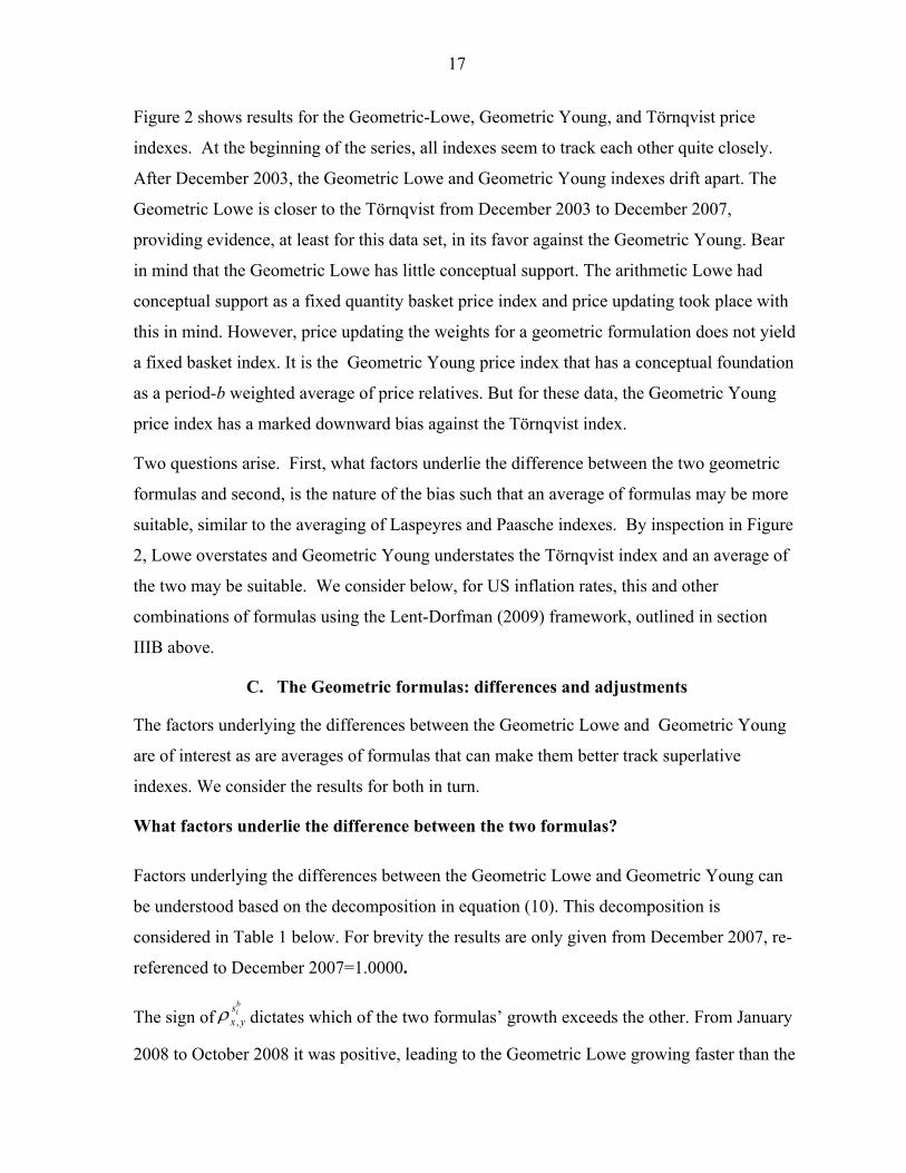
Figure 2 shows results for the Geometric-Lowe, Geometric Young, and Törnqvist price
indexes. At the beginning of the series, all indexes seem to track each other quite closely.
After December 2003, the Geometric Lowe and Geometric Young indexes drift apart. The
Geometric Lowe is closer to the Törnqvist from December 2003 to December 2007,
providing evidence, at least for this data set, in its favor against the Geometric Young. Bear
in mind that the Geometric Lowe has little conceptual support. The arithmetic Lowe had
conceptual support as a fixed quantity basket price index and price updating took place with
this in mind. However, price updating the weights for a geometric formulation does not yield
a fixed basket index. It is the Geometric Young price index that has a conceptual foundation
as a period-b weighted average of price relatives. But for these data, the Geometric Young
price index has a marked downward bias against the Törnqvist index.
Two questions arise. First, what factors underlie the difference between the two geometric
formulas and second, is the nature of the bias such that an average of formulas may be more
suitable, similar to the averaging of Laspeyres and Paasche indexes. By inspection in Figure
2, Lowe overstates and Geometric Young understates the Törnqvist index and an average of
the two may be suitable. We consider below, for US inflation rates, this and other
combinations of formulas using the Lent-Dorfman (2009) framework, outlined in section
IIIB above.
C. The Geometric formulas: differences and adjustments
The factors underlying the differences between the Geometric Lowe and Geometric Young
are of interest as are averages of formulas that can make them better track superlative
indexes. We consider the results for both in turn.
What factors underlie the difference between the two formulas?
Factors underlying the differences between the Geometric Lowe and Geometric Young can
be understood based on the decomposition in equation (10). This decomposition is
considered in Table 1 below. For brevity the results are only given from December 2007, re-
referenced to December 2007=1.0000.
The sign of ,
bis
x y dictates which of the two formulas’ growth exceeds the other. From January
2008 to October 2008 it was positive, leading to the Geometric Lowe growing faster than the

18
Geometric Young and from November 2008 onward it was negative leading to the reverse
position, as shown in Table 1. These empirical runs in signs reflect long-run trends in price
change between periods b to 0 (2004/5 to December 2007) being continued in sub-periods 0
to t (December 2007 to months up to October 2008) and then being reversed in subsequent
sub-periods (to months after October 2008). This illustrates the dependency on long-run
trends for the relative positioning of the two formulas.
The magnitude of the difference is determined by the magnitude of three factors. The
correlation coefficient is not expected to be strong given price changes in one period are to be
related to the logarithms of price changes in a subsequent one; bis
xcv is a one-off factor for
period b to 0—the higher it is, other factors equal, the larger the difference. If such
dispersion increases over time, then lags between introducing weights from the survey period
into the rebased index, between b and 0, will accentuate the difference between the two
formulas. Finally, bis
y and thus the difference between the two formulas, can be expected to
increase over time. Of note is that the three factors are multiplicative: minimize any one
factor, such as bis
xcv by minimizing the time lag in the introduction of weights, and the
difference between formulas becomes smaller. The results from Table 1 confirm this.
Averages of formulas that better track superlative indexes
An approach based on the Lent-Dorfman (2009) (hereafter L-D) framework uses averages of
two formulas to more closely correspond to a superlative index.19
In Table 2 we consider average monthly percentage differences between the target indexes
and alternative measures using the simulated US CPI data for January 2004 to December
2010. Lowe has the largest bias of about 1.7 percent from a superlative index and Young
performs much better, reducing the bias to about 0.5 percent. Their geometric equivalents
show mixed results with the Geometric Lowe being, on average, 0.2 percent above the
Törnqvist while the Geometric Young is about 1.0 percent below. We also consider
averaging of these indexes along with some variants of the L-D approach. 19 Both Fisher and Törnqvist are used as target superlative indexes, tracking each other very closely: the former has an annual growth of 2.49033 and the latter 2.49316 over the period December 198 and to December 2010.

19
First, use is made of approximations to Laspeyres and Geometric Laspeyres in equation (14)
for which real-time data would not be available in practice. We use, in turn, Lowe and Young
formulas to approximate Laspeyres and Geometric Lowe and Geometric Young formulas to
approximate Geometric Laspeyres indexes in (14); for example, one variant would be the
geometric average of the Young and Geometric Young and another, the geometric average of
the Lowe and the Geometric Young.
Second, we tailor estimates of in (15) to be based on a selected superlative benchmark,
say the Törnqvist index. The Törnqvist index cannot be estimated in real time so the most
recently available estimates are used to enable a real-time computation. For example, for
January 08 to December 2009, using our US data, the most recent estimates of Törnqvist
indexes are used, that is those available starting January 2008.
Third, the average over January 2004 to December 2005 are used in equation (15) for
January 08 to December 2009, and similarly over other periods. The Lent-Dorfman
formulation has the advantage of allowing to change on a monthly basis. However, we
constrain such changes to the period of the rebasing of the index and then hold constant
until the next rebasing. This has practical advantages: the timing of such weight changes
concurs with the rebasing of the index and CPI changes are not affected by changes in the
weight given in (14) to the different formulas used. Table 2 shows the results from using,
in equations (15) and (17), different formulas as approximations to Laspeyres and Geometric
Laspeyres benchmarked on the two superlative indexes, Fisher and Törnqvist. All
formulations can be calculated in real time using the existing prices database.
Fourth, estimates of the weights using equation (16) may be negative depending on the
relative positioning of the Geometric Young (as a proxy for the Geometric Laspeyres) and
the Young (for Laspeyres) indexes to the Fisher (superlative) index and that 0 1 .
Instead of (16) we use an adaptation, where ABS are absolute values:
0 0
0 0 0 0.
t tF CD
t t t tF CD F Y
ABS I I
ABS I I ABS I I
(17)

20
In Table 2 four different variants of the L-D formulation are given each using the Fisher and
Törnqvist indexes as benchmarks. This is preceded by the geometric mean of the two
formulas—one arithmetic one geometric—used as an approximation.
These simple geometric means are highly successful (especially for Geometric Young:Lowe
and GLowe:Young) in cutting the bias from using the Young index. The L-D
approximations have similar effects in reducing the bias. The Lowe formula is used by the
US and many other countries for CPI compilation. From Table 2 we can see that in real time
using the same database as used by Lowe, we can cut Lowe’s bias from 1.7 percent to 0.3
percent. The Geometric Young:Lowe formulation has much to commend it as an adjustment,
via the Geometric Young index, of the existing Lowe formula.
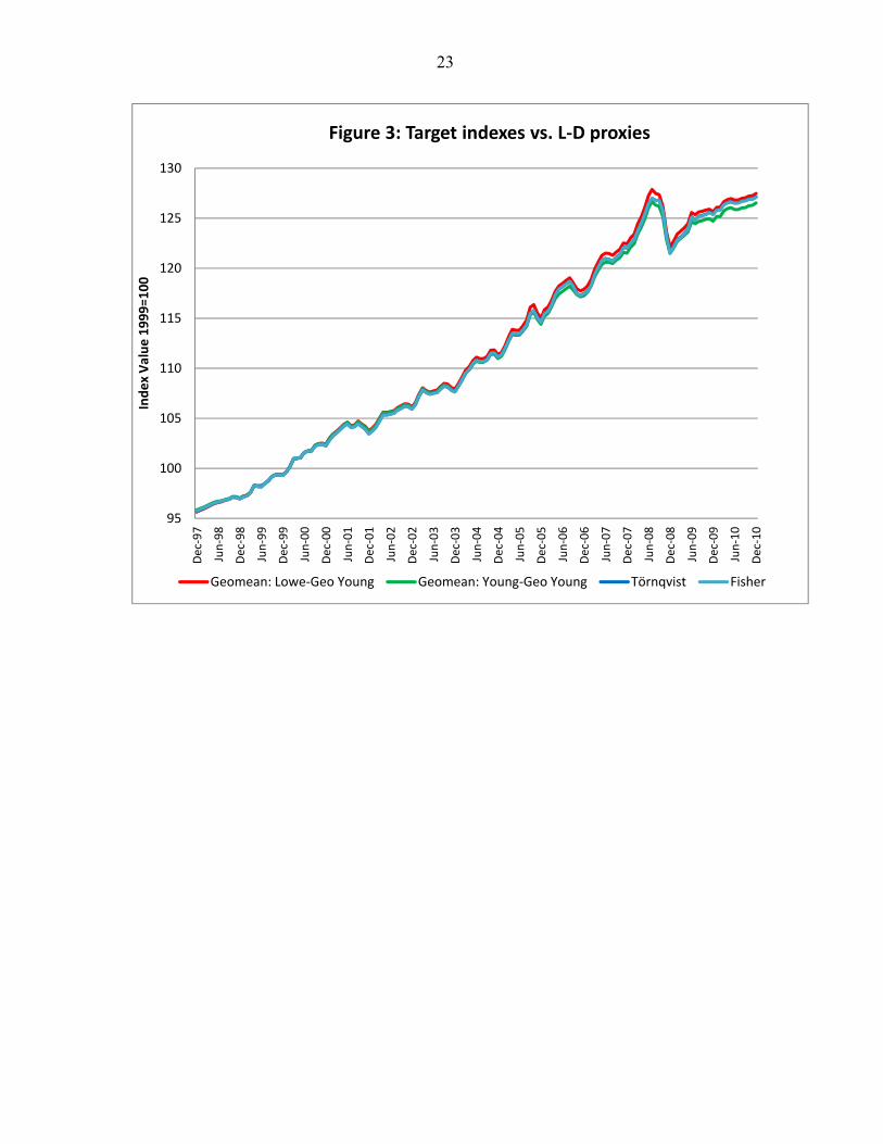
From our analysis in Figure 3, the L-D approximations (average of Lowe: Geometric Young
and average of Young:Geometric Young) to the Törnqvist and Fisher indexes appear to
work: they successfully track the Törnqvist index and alleviate the downward bias in the
Geometric Young and the upward bias in the Lowe or Young indexes. The L-D index has a
conceptual basis as a Taylor approximation to the Törnqvist (or Fisher) index that can be
calculated in real time. As Lent and Dorfman (2009) note: the systematic updating of the
index continuously picks up changes in consumer buying patterns as reflected in the data,
while requiring no iterative numerical procedures and can therefore be easily programmed
and automated in a statistical production setting.
V. CONCLUDING REMARKS
The widely-used arithmetic Laspeyres-type aggregation formula at the higher (weighted)
level for CPIs, the Young and Lowe indexes, have little justification in theory and in practice,
something of major concern for this key macroeconomic indicator. The empirical work in
Section IV used US data which benefited from relatively frequent rebasing and thus shows
only some of the potential bias that may arise from these formulas. Nonetheless, we find the
Lowe and the Young indexes to upward drift against (the already biased) Laspeyres, more so
the Lowe. The Lowe index, like Laspeyres, has the advantage of ease of interpretation as a
fixed quantity basket index. It provides a well-defined, but biased, result.
The two geometric formulations most readily available for compilers are the Geometric
Young and the Geometric Lowe price indexes. The Geometric Young is easily explained as a

21
weighted geometric average of price changes, using the survey period expenditure shares as
weights. The Geometric Lowe has no meaningful interpretation. A formal exact
decomposition of the difference between the Geometric Lowe and Geometric Young indexes
found it to be based on long-run unidirectional price changes, equations (10) and (11), the
nature of which made it unreliable as a basis for a predictable relationship between the
Geometric Lowe and a Geometric Young/Törnqvist index.
The empirical work found all indexes considered improved on the Lowe index. Averages of
geometric and arithmetic formulations were considered drawing on the L-D framework. We
found these real-time L-D indexes tracked the Törnqvist and Fisher indexes very well. Even
very simply formulations using geometric means of the two formulas were vast
improvements on other standard arithmetic and geometric formulas.
The authors are well aware of the difficulties involved in changing the CPI formula from a
long-standing and easily understood one to a more complex one. Similar issues arose when
statistical agencies moved from arithmetic formulations to the widely adopted and
conceptually sound geometric mean (Jevons index) at the lower level of CPI aggregation
(Armknecht, 1996, Silver, 2007). However, it is time to debate moving on from Laspeyres-
type indexes. One approach is to calculate retrospective indexes to identify the extent of the
substitution bias.20 Yet the CPI is a key economic indicator and users would be better served
by a real-time measure that more closely tracks a superlative index. It may well be that the
public will accept a more complex formula if it can be demonstrated that it works much
better. The Lowe index was found to have several times the bias of some of the geometric
indexes and L-D approximations that could be compiled in real time using the self-same data.
20 The US Chained Consumer Price Index for All Urban Consumers or C-CPI-U is a chained Törnqvist. Details are available at: http://www.bls.gov/cpi/.

22
100
105
110
115
120
125
130
Jan
-02
Jun
-02
No
v-0
2
Ap
r-0
3
Sep
-03
Feb
-04
Jul-
04
Dec
-04
May
-05
Oct
-05
Mar
-06
Au
g-0
6
Jan
-07
Jun
-07
No
v-0
7
Ap
r-0
8
Sep
-08
Feb
-09
Jul-
09
Dec
-09
May
-10
Oct
-10
Ind
ex
Val
ue
Figure 1: Arithmetic indexes
Lowe
Young
Lasperyres
Paasche
95
100
105
110
115
120
125
130
Dec
-97
Jun
-98
Dec
-98
Jun
-99
Dec
-99
Jun
-00
Dec
-00
Jun
-01
Dec
-01
Jun
-02
Dec
-02
Jun
-03
Dec
-03
Jun
-04
Dec
-04
Jun
-05
Dec
-05
Jun
-06
Dec
-06
Jun
-07
Dec
-07
Jun
-08
Dec
-08
Jun
-09
Dec
-09
Jun
-10
Dec
-10
Ind
ex
valu
e 1
99
9=1
00
Figure 2: Geometric vs. standard price indexes
Törnqvist Fisher Geo Lowe Geo Young Lowe Young
23
95
100
105
110
115
120
125
130
Dec
-97
Jun
-98
Dec
-98
Jun
-99
Dec
-99
Jun
-00
Dec
-00
Jun
-01
Dec
-01
Jun
-02
Dec
-02
Jun
-03
Dec
-03
Jun
-04
Dec
-04
Jun
-05
Dec
-05
Jun
-06
Dec
-06
Jun
-07
Dec
-07
Jun
-08
Dec
-08
Jun
-09
Dec
-09
Jun
-10
Dec
-10
Ind
ex
Val
ue
19
99
=10
0Figure 3: Target indexes vs. L-D proxies
Geomean: Lowe-Geo Young Geomean: Young-Geo Young Törnqvist Fisher

24
Table 1: Decomposition of Geometric-Lowe to Geometric Young ratio
GeometricGeometric- Geometric Lowe/Geometric
Young Lowe Young
,
bis
x y bis
y bis
xcv ,expb b bi i is s s
x y x ycv
2007 Dec 1 1 1
2008 Jan 1.0048 1.0052 1.0004 0.1962 0.0133 0.1712 1.0004
2008 Feb 1.0077 1.0081 1.0003 0.1039 0.0184 1.0003
2008 Mar 1.0147 1.0170 1.0023 0.4543 0.0292 1.0023
2008 Apr 1.0194 1.0232 1.0038 0.6069 0.0366 1.0038
2008 May 1.0250 1.0316 1.0065 0.7142 0.0530 1.0065
2008 Jun 1.0321 1.0414 1.0091 0.7324 0.0719 1.0091
2008 Jul 1.0367 1.0467 1.0096 0.6892 0.0809 1.0096
2008 Aug 1.0356 1.0434 1.0075 0.6390 0.0685 1.0075
2008 Sep 1.0355 1.0423 1.0066 0.6256 0.0612 1.0066
2008 Oct 1.0294 1.0315 1.0021 0.2621 0.0469 1.0021
2008 Nov 1.0139 1.0064 0.9927 -0.5619 0.0767 0.9927
2008 Dec 1.0031 0.9900 0.9869 -0.6632 0.1159 0.9869
2009 Jan 1.0077 0.9959 0.9883 -0.6329 0.1089 0.9883
2009 Feb 1.0131 1.0026 0.9897 -0.6119 0.0987 0.9897
2009 Mar 1.0156 1.0051 0.9897 -0.6074 0.0998 0.9897
2009 Apr 1.0178 1.0085 0.9909 -0.5676 0.0943 0.9909
2009 May 1.0203 1.0133 0.9932 -0.3853 0.0845 0.9944
2009 Jun 1.0275 1.0248 0.9974 -0.2102 0.0725 0.9974
2009 Jul 1.0259 1.0226 0.9968 -0.2383 0.0779 0.9968
2009 Aug 1.0276 1.0255 0.9979 -0.1581 0.0766 0.9979
2009 Sep 1.0284 1.0256 0.9973 -0.2025 0.0794 0.9973
2009 Oct 1.0298 1.0266 0.9969 -0.2312 0.0785 0.9969
2009 Nov 1.0300 1.0281 0.9981 -0.1457 0.0747 0.9981
2009 Dec 1.0280 1.0259 0.9979 -0.1589 0.0766 0.9979

25
Table 2, Average Monthly Percentage Differences between Alternative vs. Target Indexes:*
Target Indexes
Fisher Törnqvist
Arithmetic formulas
Lowe 1.712 1.689
Young 0.466 0.443
Geometric formulas
Geometric Lowe (GLowe) 0.265 0.242
Geometric Young -0.959 -0.981
Geometric means of formulas
GYoung-Young -0.249 -0.272
GYoung-Lowe 0.368 0.345
GLowe:Young 0.366 0.343
GLowe:Lowe 0.986 0.963
Lent-Dorfman (η using lag)
GYoung:Young -0.339 -0.375
GYoung:Lowe -0.196 -0.219
GLowe:Young 0.339 0.316
GLowe:Lowe 0.581 0.558
*Covers January 2004 to December 2010

26
References Armknecht, Paul A., (1996), “Improving the Efficiency of the U.S. CPI,” IMF Working Paper
WP/96/103, (International Monetary Fund, Washington, D.C,), September.
Balk, Bert M., (1983), “Does There Exist a Relation Between Inflation and Relative Price Change Variability? The Effect of the Aggregation Level” Economic Letters, 13, 173-80.
Balk, Bert. M., (2010), “Lowe and Cobb-Douglas Consumer Price Indices and their Substitution Bias,” Jahrbücher für Nationalökonomie und Statistik, Vol. 230, No. 6, 726-740. Balk, Bert M. and W. Erwin Diewert, (2003), “The Lowe Consumer Price Index and its Substitution Bias,” Discussion Paper No. 04-07 (Department of Economics, University of British Columbia, Vancouver). Ball, Laurence, and N. Gregory Mankiw, (1995), “Relative-Price Changes as Aggregate Supply Shocks,” Quarterly Journal of Economics 110, 161–193. Bortkiewicz, L.v., (1923), “Zweck und Struktur einer Preisindexzahl,” Nordisk Statistisk Tidsskrift , 2, 369–408. Feenstra, Robert C., and Marshall B. Reinsdorf, (2007), “Should Exact Index Numbers Have Standard Errors? Theory and Application to Asian Growth,” in Hard-to-Measure Goods and Services: Essays in Honor of Zvi Griliches (Ernst R. Berndt and Charles R. Hulten, eds.). National Bureau of Economic Research, October. Glejser, Herbert, (1965). “Inflation, Productivity, and Relative Prices: A Statistical Study,” Review of Economics and Statistics 47, 76–80. Greenlees, John S., (2011), “Improving the Preliminary Values of the Chained CPI-U,” Proceedings of the Business and Economic Statistics Section, Journal of Economic and Social Measurement, 31, 1-2, 1-18. Greenlees, John S. and Elliot Williams, (2010), “Reconsideration of Weighting and Updating Procedures in the U.S. CPI,” Jahrbücher für Nationalökonomie und Statistik, 230, 6, 741-758.. Hansen, Carsten Bolden, (2007), “Recalculations of the Danish CPI 1996 – 2006,” Proceedings of the Tenth Meeting of the International Working Group on Price Indexes, (Ottawa, Canada). Available at: www.ottawagroup.org. Hercowitz, Zvi, (1982), “Money and Price Dispersion in the United States,” Journal of Monetary Economics 10, 25–37. International Labour Office (ILO), IMF, OECD, Eurostat, United Nations, World Bank, (2004), Consumer Price Index Manual: Theory and Practice, (Geneva: ILO). http://www.ilo.org/public/english/bureau/stat/guides/cpi/index.htm. Lastrapes, W.D., (2006) “Inflation and the Distribution of Relative Prices: The Role of Productivity and Money Supply Shocks,” Journal of Money, Credit, and Banking, 38, 8, December, 2159-2198 Lent, Janice, and Alan H. Dorfman, (2009). “Using a Weighted Average of Jevons and Laspeyres Indexes to Approximate a Superlative Index,” Journal of Official Statistics 25, 1, 129–149.

27
Pike, Chris, (2009), “New Zealand 2006 and 2008 Consumers Price Index Review: Price Updating,” Room document, Eleventh Meeting of the International Working (Ottawa) Group on Price Indexes, Neuchatel, Switzerland, May. Available under “Papers” at: http://www.ottawagroup.org/. Reinsdorf, Marshall B., (1994), “New Evidence on the Relation and Price Dispersion” American Economic Review 84, 3,720-731. Silver, Mick and Saeed Heravi (2007), “Why Elementary Price Index Number Formulas Differ: Price Dispersion and Product Heterogeneity,” Journal of Econometrics, 140, 2, 874–83.
Silver, Mick and Christos Ioannidis, C., (2001), “Inter-Country Differences in the Relationship Between Relative Price Variability and Average Prices,” Journal of Political Economy, 109, 2, 355-374, April.
United Nations Economic Commission for Europe (UNECE), ILO, IMF, OECD, Eurostat, World Bank, Office for National Statistics United Kingdom, (2009), Practical Guide to Producing Consumer Price Indices (New York and Geneva: United Nations): http://www.imf.org/external/data.htm#guide.
Van Hoomisson, T., (1988), “Price Dispersion and Inflation: Evidence from Israel,” Journal of Political Economy, 96, 6, 1303-1314.
Vining, Daniel R., Jr., and Thomas C. Elwertowski, (1976), “The Relationship between Relative Prices and the General Price Level,” American Economic Review 66, 699–708.


