
POLYATOMIC ANION CONDUCTION IN Sc2(WO4)3
TYPE STRUCTURES
BY
ZHOU YONGKAI
(B. Eng., Beihang Univ.)
A THESIS SUBMITTED
FOR THE DEGREE OF DOCTOR OF PHILOSOPHY
DEPARTMENT OF MATERIALS SCIENCE &
ENGINEERING
NATIONAL UNIVERSITY OF SINGAPORE
2010

To my parents
To everyone who is striving for a doctorate

i
Acknowledgements
Finally this thesis is almost done and it is time to finish the last piece of work of
the huge project. I have to thank many people who have witnessed the last and most
important work of my student’s life.
First of all, I would like to express my wholehearted gratitude to my supervisor,
Dr. Stefan Adams, for providing me with the wonderful opportunity to pursue my
PhD degree. I am grateful to his invaluable advice, support, detailed instructions and
guidance throughout of years of my study. It was extremely pleasant to be working
with him.
Another important person that I am grateful to is Professor Arkady Neiman from
Chemical Department of Ural State University. He is one of our collaborators working
on the polyatomic anion conduction issues. Thank him for hosting my visiting to his
lab in Russia. It was a great time to learn and work with him on the Tubandt
experiment which provided very important evidence to prove anion conduction in

ii
Sc2(WO4)3 type oxides. I am also gratitude and appreciate the friendship to two
students in Prof. Neiman’s group, Natalie and Denis. It was a pleasure to work and
have fun with them! In the meanwhile, I also appreciate the discussion on preparing
high density samples and impedance measurement with our other collaborator Prof.
Doreen Edwards as well as her two students Kara and Brittany from Alfred
University.
My sincere thanks to Dr. Zhang Xinhuai in computer center of NUS, who helped
me a lot provide technical support in using the computational recourses of university,
especially Cerius2 and Materials Studio simulation systems. I would also like to
extend my heartfelt thanks to our department staffs, Chen Qun, Mr. Chan, Agnes and
Roger. My work could not be done without their support, training and guidance for
utilizing the technical facilities.
I will take this opportunity to appreciate the friendship and support from my
group colleagues Dr. Prasada Rao, Thieu Duc Tho and Li Kangle. Especially thanks
to Dr. Prasada Rao who taught me some electrochemical techniques and offered me
fruitful discussions and inspirations on some ionic conduction theories. I will also
extend my thanks to my many other friends Yuan Du, Han Zheng, Ran Min, Hu
Guangxia, Zheng Jun, etc, who have profound influence on me.
I would like to thank the A-Star SERC to the Materials World network project no.
062 119 0009 for the financial support and National University of Singapore for
supplying me with an excellent research environment.
Last, but not least, I am especially grateful to my parents for their unconditional
love, encouragement and support.

iii
Table of Contents
Acknowledgements .......................................................................................................i
Table of Contents ....................................................................................................... iii
Summary.....................................................................................................................vii
List of Tables.................................................................................................................x
List of Figures.............................................................................................................xii
List of Publications / Conferences ...........................................................................xix
Chapter 1 Introduction................................................................................................1
1.1 Background of solid state ionics ........................................................................1
1.1.1 Definition and classification ..............................................................1
1.1.2 History................................................................................................5
1.1.3 Defects and conduction mechanism.................................................10
1.1.4 Fundamentals of diffusion and ionic conduction.............................14
1.1.5 Factors influencing ionic conductivity.............................................18
1.2 Review of earlier studies on Sc2(WO4)3 type oxides .......................................20
1.2.1 The structure of Sc2(WO4)3 type oxides .................................................20
1.2.2 Review of conduction mechanism models proposed in the literature ....22

iv
1.3 Motivation and objectives of this thesis...........................................................24
References....................................................................................................................26
Chapter 2 Research Techniques................................................................................35
2.1 Introduction............................................................................................................35
2.2 Synthesis techniques ..............................................................................................36
2.3 Experimental characterization ...............................................................................37
2.3.1 X-ray powder diffraction and Rietveld refinement.................................37
2.3.2 Impedance spectroscopy .........................................................................39
2.3.3 Scanning electron microscopy ................................................................44
2.4 Tubandt-type electrolysis experiment ....................................................................44
2.5 Atomistic simulations.............................................................................................46
2.5.1 Molecular Dynamics simulations ...........................................................46
2.5.2 Mott-Littleton calculations......................................................................50
2.6 Bond Valence analyses...........................................................................................51
References....................................................................................................................55
Chapter 3 Discovery of Polyatomic Anion Diffusion in Solid Sc2(WO4)3 .............58
3.1 Introduction............................................................................................................58
3.2 Methods..................................................................................................................59
3.2.1 Experimental ...........................................................................................59
3.2.2 Computer simulations .............................................................................61
3.3 Results and discussion ...........................................................................................62
3.3.1 Non-ambient XRD and structure refinement..........................................62
3.3.2 Computational and experimental studies of the dynamic structure ........68
3.3 Mass and charge transfer experiments in Tubandt-type cells with Sc2(WO4)3......87
3.4 Conclusions............................................................................................................93

v
References....................................................................................................................94
Chapter 4 Intrinsic Polyatomic Defect Formation and Transport in Solid
Scandium Tungstate Type Oxides.............................................................................96
4.1 Introduction............................................................................................................96
4.2 Methods..................................................................................................................98
4.2.1 Defect energy calculations and electron density mapping......................98
4.2.2 Polyanion migration in defected structures.............................................98
4.2.3 Experimental .........................................................................................100
4.3 Results and discussion .........................................................................................100
4.3.1 Intrinsic defects.....................................................................................100
4.3.2 Migration energies ................................................................................106
4.3.3 Experimental characterization of nonstoichiometric samples ..............113
4.4 Conclusions..........................................................................................................118
References..................................................................................................................119
Chapter 5 Polyanion Transport at Nanostructured Interfaces............................121
5.1 Introduction..........................................................................................................121
5.2 Methods................................................................................................................123
5.3 Results and discussion .........................................................................................124
5.3.1 Forcefield for this simulation................................................................124
5.3.2 Surface energy calculation....................................................................125
5.4 Conclusions..........................................................................................................136
References..................................................................................................................137
Chapter 6 Conclusion and Future Work ...............................................................139
6.1 Conclusion ...........................................................................................................139
6.2 Future directions ..................................................................................................142

vi
References..................................................................................................................145
Appendix...................................................................................................................146

vii
Summary
This thesis studies the conduction mechanism of Sc2(WO4)3 as the prototype of a
large class of oxides with general formula R2(MO4)3 (where R = Sc, In, Al, rare earth
ions, …; M=W and Mo). Combined electrochemical and diffraction experiments and
computer simulations are employed in this study to comprehensively investigate their
structures, ionic conductivities, ion diffusion pathways, defect formation energies and
dynamic behaviour of each species in the structure.
Chapter 1 is a general introduction to the area of solid state ionics (SSI).
Historical development, basic classifications, factors affecting the ionic conductivities,
point defect conduction mechanisms and basic diffusion theories of SSI are described.
Literature on the structure and properties of Sc2(WO4)3-type oxides and especially the
trivalent cation conduction hypothesis are reviewed comprehensively. Finally,
motivation and objectives of this thesis are presented.
Chapter 2 briefly explains experimental techniques and computer simulation

viii
methods that are used in this study. Experimental techniques include sample
preparation, in situ X-ray diffraction, impedance characterization, scanning electron
microscopy and Tubandt-type electrolysis experiments. The computer simulation
methods include Molecular Dynamics (MD) simulations, Mott-Littleton calculations
and Bond Valence calculations.
Chapter 3 presents the results of X-ray Diffraction (XRD) structural studies
focusing on the negative thermal expansion and variations of the apparent bond
lengths with temperature, as well as the characterization of the (ionic) conductivity
Sc2(WO4)3 by impedance spectroscopy. A modified universal forcefield (UFF) for
MD simulations successfully reproduces the negative thermal expansion behaviour
over a limited temperature range. The hopping diffusion process of WO42− group is
directly observed in Isothermal−Isobaric ensemble (NPT) simulations with the same
modified UFF. The hopping traces of WO42− group follow the pathway predicted by
bond valence analyses for MD simulation trajectories. Tubandt experiment supports
anion conduction in Sc2(WO4)3. The combination of experimental and computational
information then leads to the identification of the ion transport mechanism.
In Chapter 4 the observed novel polyanion ion transport mechanism is
investigated more in detail. It starts with a characterization of the formation energies
of various potential atomic defects in Sc2(WO4)3 by the Mott-Littleton method. It is
found that a WO42− group is energetically favorable over distributed W6+ and O2−
defects. In this way, Sc2(WO4)3 Schottky defect formation energy could be
recalculated as 1.97 eV compared to 8.91 eV if each vacancy is regarded as isolated
defect. Among the calculated defect energies the value for WO42− anti-Frenkel defects
(1.23 eV) is the lowest one. The formation energies of these Anti-Frenkel and
Schottky defects are both considerably smaller than for other conceivable defects; and

ix
thus they can be self generated. The migration energies of individual WO42−
interstitial and vacancy are estimated by MD simulations to be 0.68 and 0.74 eV, both
of which are very close to experimental value 0.67 eV. Considering that the mobility
of the interstitial is about one order of magnitude higher than that of a vacancy, the
WO42− interstitial is expected to be the dominant mobile defect in Sc2(WO4)3.
In Chapter 5, the diffusion behaviour of WO42− polyatomic anions at the
nanoscale heterostructure interfaces are investigated by MD simulations. The
structures of both phases near the interface become disordered; therefore, polyatomic
anion conductivity is enhanced by introducing heterointerfaces.
Chapter 6 concludes this thesis and suggests future application of polyatomic
anion conductor for sensors.

x
List of Tables
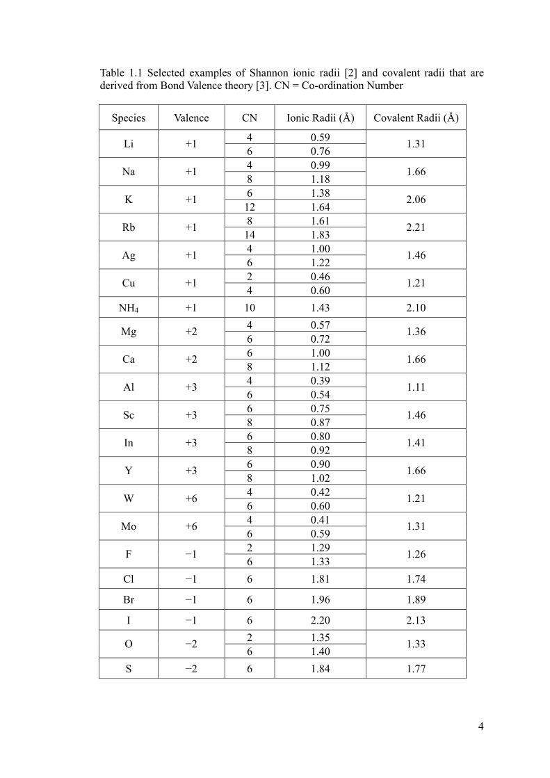
Table 1.1 Selected examples of Shannon ionic radii [2] and covalent radii that are
derived from Bond Valence theory [3]. CN = Co-ordination Number ..........................4
Table 1.2 Selected examples of ionic conductors ..........................................................7
Table 1.3 Selected examples of disorder types and mobile defects. Ref. [15, 101] ....14
Table 2.1 Capabilities of methods for the conduction pathway analysis, reproduced
from Ref. [23] ..............................................................................................................52
Table 3.1 Cell Dimensions as a Function of Temperature ...........................................63
Table 3.2 Linear thermal expansion coefficients for lattice constants a – c and
expansion coefficient of the unit cell volume V ..........................................................64
Table 3.3 Mass changes for 4 Tubandt experiments ....................................................89
Table 4.1 Calculated defect formation energies.........................................................106

xi
Table 4.2 Comparison of calculated Frenkel and Schottky defects energies from
Driscoll’s work and this work ....................................................................................106
Table 4.3 Comparison of calculated and experimental energies................................110
Table 5.1 Experimental [20] and calculated structural parameters of CaWO4 at room
temperature. ...............................................................................................................124
Table 5.2 Experimental [21] and calculated elastic constants of CaWO4 at room
temperature. ...............................................................................................................124
Table 5.3 Calculated surface energies (γ) of Sc2(WO4)3 and CaWO4. Different
terminations of Sc2(WO4)3 (0 1 0) surface (as indicated in Figure 5.1) and CaWO4 (1 0
1) surface (see Figure 5.2) are compared...................................................................126
Table 5.4 Heterostructure building strategy. ..............................................................129
Table A.1 Atomic fraction coordinates of Sc2(WO4)3 at 11 to 1300K. ......................146

xii
List of Figures
Figure 1.1 Arrhenius plots of conductivity for selected crystalline (a) silver conductors,
(b) proton conductors, (c) other cation conductors (Li+, Na+, Cu+) and (d) anion
conductors (O2−, F−). Reproduced from Ref. [101]. ......................................................9
Figure 1.2 Illustration of Frenkel defect (a) and Schottky defect (b). .........................11
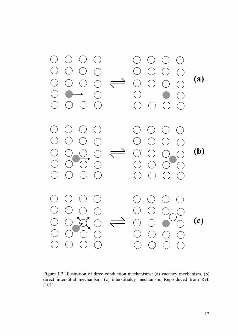
Figure 1.3 Illustration of three conduction mechanisms: (a) vacancy mechanism, (b)
direct interstitial mechanism, (c) interstitialcy mechanism. Reproduced from Ref. [101].
......................................................................................................................................12
Figure 1.4 Illustration of the Grotthuss conduction mechanism for H+.......................13
Figure 1.5 Projection of the Sc2(WO4)3 structure on the a b plane showing (a) ScO6 as
light octahedra; W(1)O4 as dark and W(2)O4 as light tetrahedra (O not shown) (b) Sc as
large, O as small spheres and WO4 tetrahedra as in graph (a). From the observations
reported in this work, it appears to be more appropriate to use version (b) emphasizing
the WO42− groups as structural units............................................................................21

xiii
Figure 2.1 Inverted crucible technique for making Sc2(WO4)3 powders.....................36
Figure 2.2 Nyquist Plot with Impedance Vector after Barsoukov et al. [8].................42
Figure 2.3 Nyquist plot of impedance of a solid electrolyte with ion blockage electrode
system. Zre represents real part of the impedance, while Zim is the imaginary part.....43
Figure 2.4 Equivalent circuit of Figure 2.3 with mixed kinetic and charge transfer
control. W is called Warburg impedance [12, 13]........................................................43
Figure 2.5 Tubandt experiment setup with 3 disks between Pt electrodes. .................45
Figure 2.6 Time dependence of current in the Tubandt experiment. ...........................45
Figure 2.7 Trajectory of a particle in MD simulation ..................................................48
Figure 2.8 Periodic boundary conditions after Côté et al. [18]....................................49
Figure 2.9 Illustration of the two-region dividing strategy in Mott-Littleton method.51
Figure 2.10 Ag+ conduction pathways in α-AgI after Adams et al. [27] .....................54
Figure 3.1 Refinement of Sc2(WO4)3 structure at 300K with final Rwp=5.96%. Observed
(×), calculated (line), and Observed − calculated (lower line). The inset shows the
details of the refinement result in the 2 theta range from 18° to 31°. ..........................64
Figure 3.2 Temperature dependence of (a) unit cell parameters and (b) cell volume of
Sc2(WO4)3 as determined from high temperature (▲) or low temperature (■) XRD data
in this work. Neutron diffraction data by Evans [1] (○) are shown for comparison....65
Figure 3.3 Temperature dependence of (a) the average apparent bond length and (b) of
the atomic displacement parameters in Sc2(WO4)3 as determined from Rietveld
refinements...................................................................................................................67
Figure 3.4 Schematic representation of how the negative thermal expansion can be

xiv
linked to the increase in amplitude of a rocking mode of nearly rigid building blocks.
Top: dark WO4 tetrahedron, bottom light grey ScO6 octahedron; O shown as spheres.
The average W – Sc distance (dotted line) drops from 3.776 Å at 50K to 3.758 Å at
1000K...........................................................................................................................70
Figure 3.5 Variation of lattice constants a (squares), c (triangles) and b (circles) of
Sc2(WO4)3 as a function of temperature in a NPT simulation (solid) which are
compared with experimental data (hollow) from this work.........................................71
Figure 3.6 Variation of the angle α with time in an isothermal−isobaric (NPT)
simulation for the pressure p = 0.9 GPa.......................................................................73
Figure 3.7 Comparison of simulated lattice constants and monoclinic angle α as a
function of pressure with experimental literature values [2]: (a), (b) and (c) normalized
lattice constants. (d) monoclinic angle α. For all pressures the (pseudo-) orthorhombic
setting has been chosen to emphasise the structural relationship of the high and low
pressure phases. Experimental values: grey symbols; simulated values: black symbols.
The low pressure orthorhombic phase is marked by filled squares and the high pressure
monoclinic phase by open squares...............................................................................75
Figure 3.8 The trace of the motion of (a) W atoms (initial positions of the nine moving
WO42− groups indicated as circles; the first hop from an equilibrium site to an
interstitial tungstate site is marked by an arrow) and (b) Sc atoms for the NVT
simulation of Sc2(WO4)3 at T=1300K..........................................................................77
Figure 3.9 “Rock and roll” transport mechanism for tungstate ions in Sc2(WO4)3.
Graphs (a) - (f) show an elementary transport process from details of snapshots from 5
ps of a 5 ns MD simulation (T =1300 K). The direction of motion is highlighted by
arrows. A regular WO42− ion A (shown as ball and stick) reorients under the influence
of an approaching interstitial WO42− ion B (shown as grey tetrahedron), (a) and then
rolls to an interstitial position (b, c). After a further reorientation step (d) ion B fills the
site previously occupied by A (e, f). ............................................................................78
Figure 3.10 (a) Simulated mean square displacement of WO42− and Sc3+ vs. time for a

xv
NVT simulation of Sc2(WO4)3 at T = 1300K. (b) Comparison of simulated conductivity
(■), experimental conductivities obtained in this work (□). Experimental data by
Driscoll et al. [17] (●) and by Imanaka et al. [18] (▲) are shown for comparison. The
inset graph shows the variation of the activation energy with temperature as derived
from the three sets of experimental conductivity data (using the same symbols). ......80
Figure 3.11 Correlation between the variation of the distance of a WO42− (with respect
to its position at t0 = 3400 ps) and the change in the orientation angle of two W-O bonds
(with respect to the x axis) over 69 ps with a resolution of 0.1ps................................82
Figure 3.12 Four selected frames from a dynamic bond valence analysis with nine
moving WO42− groups (marked by grey spheres) forming a pathway through the
supercell (total time interval between frames (a) t = 3403.3ps and (d) t = 3404.5ps is 1.2
ps). The grey isosurface represents a BVS model of the instantaneous WO42− pathways
(i.e. regions of BVS mismatch |V| < 0.25 valence units for WO42−). Traces of the W
atoms that hop within a 69 ps period of the MD simulation (same period as for Figure
3.11) are superimposed on this BVS pathway landscape. Arrows mark the position of
the first moving ion during the defect creation process. In contrast to the series of
subsequent hops it does not follow the low energy transport pathway........................85
Figure 3.13 Schematic setup of Tubandt-type cell experiments with stacks of 3
Sc2(WO4)3 disks for T = 940°C . Average mass changes and their standard deviations
are indicated for the individual disks as observed in the four experiments listed in Table
3.3.................................................................................................................................89
Figure 3.14 Tubandt-type electrolysis experiments with stacks of 2 Sc2(WO4)3 disks for
T = 940°C . Mass change of each disk is indicated. ....................................................90
Figure 3.15 Low angle XRD profile for (a): boundary (1) and (b): boundary (4) as
shown in Figure 3.14. Diffraction peaks corresponding to Sc6WO12 and WO3 phases are
indicated on the graphs. ...............................................................................................91
Figure 4.1 Structure model of Sc2(WO4)3 projected along Z axis (a) and X axis (b). One
interstitial site for WO42− is marked as a black sphere. W(1)O4 shown as dark and

xvi
W(2)O4 shown as light gray tetrahedra, Sc gray cross..............................................102
Figure 4.2 Electron density map for Sc2(WO4)3 projected along Z axis (a) and X axis (b).
The grey isosurfaces enclose regions with electron density > 0.42 Å−3. W shown as dark
spheres, Sc as gray spheres, W-O bond as sticks. ......................................................103
Figure 4.3 Detail from the relaxed structure of Sc2(WO4)3 with one interstitial WO42−
defect (black tetrahedron) projected along Z axis (a) and X axis (b). WO42−
corresponding to one unit sell in Figure 4.1 are shown as dark gray tetrahedra, others
are shown as light tetrahedra, Sc gray cross. .............................................................104
Figure 4.4 Comparison of experimental conductivity with simulated conductivities for
the two different defect models discussed in the text. ...............................................107
Figure 4.5 Trace of WO42− group motion over 200 ps in the 1250 K MD simulation for
structure model (ii) with an artificially induced Frenkel-defect. The position of the
initial interstitial is marked by ; the initial vacancy by an open circle. (Projection
along z-axis)...............................................................................................................109
Figure 4.6 Comparison of experimental conductivity and simulated conductivities for
Sc2(WO4)3 structure models containing one extra interstitial tungstate, tungstate
vacancy, or initially no defect. ...................................................................................110
Figure 4.7 Traces of the motion of (a, c) tungstate groups (represented by W atoms) and
(b, d) Sc atoms for the NVT simulation of Sc2(WO4)3 structures with (a, b) vacancy
defect and (c, d) interstitial defect, based on 15 snapshots over 5 ns period at T=1300K.
....................................................................................................................................112
Figure 4.8 Comparison of experimental conductivities of nonstoichiometric samples
with formula Sc2O3 − xWO3, where x = 2.9, 3.0 and 3.1. For all samples of this study
the activation energies are 0.66eV±0.02eV. The deviating high temperature behaviour
for the sample from the previous study [1] might be affected by the differences in the
thermal history of the samples and the different nature of the electrodes. ................114
Figure 4.9 SEM photographs of Sc2(WO4)3 samples with different density: (a) 70% of

xvii
theoretical density prepared by this work, (b) and (c) are prepared by Prof. Edwards’
group with density of 74% and 91% respectively......................................................117
Figure 4.10 Impedance spectra of two samples at 600 °C: (a) sintered under applied
pressure with 91% of theoretical density, (b) sintered with no pressure with 74% of
theoretical density. .....................................................................................................117
Figure 4.11 Comparison of this work’s experimental conductivities of stoichiometric
samples with Edwards’ work. ....................................................................................118
Figure 5.1 Three terminations of (0 1 0) plane in the Sc2(WO4)3 unit cell, which is
shown in the projection along z axis, showing Sc as large, O as small spheres and WO4
tetrahedra....................................................................................................................126
Figure 5.2 Two terminations of (1 0 1) plane in the CaWO4 unit cell, which is shown in
the projection along z axis, showing Ca as large, O as small spheres and WO4 tetrahedra.
....................................................................................................................................127
Figure 5.3 Illustration of the relaxation scheme for the heterostructure. The initial
structure (left) is first geometry optimized and then fully relaxed in the NPT
simulations at 600K for 100 ps. W atoms are shown as tetrahedra (Gray ones originally
belong to CaWO4, while dark ones belong to Sc2(WO4)3.), Sc as gray spheres, Ca as
dark spheres in the structure. .....................................................................................130
Figure 5.4 Accumulated number of atoms, started from the bottom of the shown
structure, of each element. W atoms are shown as tetrahedra (Gray ones originally
belong to CaWO4, while dark ones belong to Sc2(WO4)3.), Sc as gray spheres, Ca as
dark spheres in the structure ......................................................................................131
Figure 5.5 Variation of the WO42− diffusion coefficient against the distance from the
interface. (a) is the total diffusion coefficient; while (b), (c) and (d) are anisotropic
diffusion coefficients in x, y and z directions respectively. Squares correspond to the
“upper interface”, while triangles indicate the “lower interface”. The vertical line
indicates the center of the interface, while the horizontal dashed line represents the

xviii
experimental bulk diffusion coefficient at 600K. ......................................................134
Figure 5.6 Comparison of experimental conductivity and simulated conductivities for
Sc2(WO4)3 structure models containing one extra interstitial tungstate, tungstate
vacancy, initially no defect and Sc2(WO4)3 at heterointerface. .................................135
Figure 6.1 Cross−sectional view of the CO2 sensor cell. Reproduced from Ref [2]. 143
Figure 6.2 Design of a WO42− concentration sensor based on WO4
2− solid electrolytes.
....................................................................................................................................145
Figure 6.3 Design of a WO3 gas sensor based on WO42− solid electrolytes. .............145
Figure A.1 Refinement of Sc2(WO4)3 structure at (a) 800K with final Rwp=6.03% and (b)
1300K with final Rwp=6.06%. Observed (×), calculated (line), and Observed −
calculated (lower line). The insets show the details of the refinement result in the 2 theta
range from 18° to 31°. ..……………………………………………………………..154
Figure A.2 XRD profiles of Sc2(WO4)3 structure from 100K to 1300K: (a) shows the
full range profiles from 12° to 120°, while (b) shows details in the range from 18° to
31°. ………………………………………………………………………………….155

xix
List of Publications / Conferences
Publications / Conference Papers
1. Yongkai Zhou, Arkady Neiman, Stefan Adams, "Novel polyanion conduction
in Sc2(WO4)3 type negative thermal expansion oxides", Physica Status Solidi B,
in press, DOI: 10.1002/pssb.201083969.
2. Yongkai Zhou, R. Prasada Rao, Stefan Adams, "Intrinsic polyatomic defects in
SC2(WO4)3", Solid State Ionics, in press, DOI: 10.1016/j.ssi.2010.06.024.
3. Yongkai Zhou, Stefan Adams, Arkady Neiman, "Polyanion Conduction
Mechanism in Solid Scandium Tungstate", Mater. Res. Soc. Symp. Proc. 1177E
(2009) Z09-20.
4. Yongkai Zhou, R. Prasada Rao, Stefan Adams, "Charge Transport by
Polyatomic Anion Diffusion in Sc2(WO4)3", Chemical Monthly, 140 (2009)
1017–1023.
5. Yongkai Zhou, Stefan Adams, R. Prasada Rao, Doreen D. Edwards, Arkady
Neiman, N. Pestereva, "Charge transport by polyatomic anion diffusion in
Sc2(WO4)3", Chemistry of Materials, 20 (2008) 6335–6345.

xx
Oral Presentations in International Conferences
1. Yongkai Zhou, Stefan Adams, "Novel Polyanion Conduction in Negative
Thermal Expansion Sc2(WO4)3Type Oxides", 6th International Workshop on
Auxetics and Related System: Bolton, UK, 14-17 September 2009.
2. Yongkai Zhou, Stefan Adams, "Mechanism of Polyanion Transport in Oxides
with the Scandium Tungstate Structure", The 17th International Conference
on Solid State Ionics: Toronto, Canada, 28 June - 3 July 2009.
3. Neiman*, A, N Pestereva, D Nechaev, D Edwards, YK ZHOU and S. Adams,
"Novel data on Transport and Reaction processes in Me2(WO4)3 (Me = Sc, In)".
ECSSC XII European Conference on Solid State Chemistry (2009).
Germany.
4. Adams*, S., PRASADA RAO R, YK ZHOU, A Neiman and DD Edwards,
"Polyatomic anions as mobile species in solid electrolytes.". Materials
Research Society Fall Meeting 2008, 1 - 5 Dec 2008, Hynes Convention
Center, Boston, United States.
5. S. Adams, Y.K. Zhou, T.Kulikova, A. Neiman, B. Riley and D. Edwards, "A
fresh look at ion transport in trivalent cation tungstates". Pro. 99th Bunsen
Kolloquium Solid State Reactivity. From Macro to Nano (7-9 Jun 2007,
Monastery Eberbach, Eberbach, Germany), p. 20 (oral).
6. T. Kulikova, A. Neiman, S. Adams, Y.K. Zhou, B. Riley and D. Edwards;
"Ionic conduction in trivalent cation tungstates: Al2(WO4)3, In2(WO4)3 and
Sc2(WO4)". Proc. 16th International Conference on Solid State Ionics SSI-16
(1-6 July 2007, Shanghai Wordfield Convention Hotel, Shanghai, China), p. 85
(oral).

xxi
Posters in International Conferences
1. Yongkai Zhou, Stefan Adams, Arkady Neiman, "Polyanion Conduction
Mechanism in Solid with Sc2(WO4)3 Structure ", 1st Singapore-Hong Kong
Bilateral Graduate Student Congress: Singapore, 28-30 May 2009.
2. Yongkai Zhou, Stefan Adams, Arkady Neiman, " Polyanion Conduction
Mechanism in Solid Scandium Tungstate", 2009 Materials Research Society
(MRS) Spring Meeting: San Francisco, CA, USA, 14-17 April 2009.
3. Yongkai Zhou, R. Prasada Rao, Stefan Adams, "Ionic conduction by
polyanions in solids with Sc2(WO4)3 structure", 3rd Materials Research
Society – Singapore (MRS-S) Conference on Advanced Materials: Singapore,
25-27 February 2008.

1
Chapter 1
Chapter 1 Introduction
1.1 Background of solid state ionics
1.1.1 Definition and classification
This research project deals with the charge transport mechanism in Sc2(WO4)3
type oxides, which are known to be solid state ionic conductors, but the ion
conducting species and the ion transport mechanism have been the matter of intense
discussion. Solid state ionic conductors, as the name suggests, are materials which can
conduct electricity by the migration of mobile ions (cations and/or anions). While in
general both liquids and solids could be ionic conductors, the objective of this project

2
concentrates on solid state ionic conductors which are also called fast ion conducting
(FIC) solids. Solid ionic conductors differ from electron conductors, e.g. metals and
semiconductors, in terms of the mobile charge carriers. Both electronic and ionic
conductors are very important materials in our daily lives. Batteries and fuel cells
require both purely ionic conduction in the (solid or liquid) electrolyte phase and
electronic conductors or more commonly mixed electronic and ionic conductors as the
electrode materials. Reduction and oxidation (redox) reactions occur at the interface
between ionic conductors and electrodes to convert ionic conduction into electronic
conduction. The advantage of mixed conductors (e.g. LixCoO2) is that this charge
transfer reaction can also occur inside a mixed conducting electrode, while for purely
electronic conductors the transfer is restricted to the interface itself.
Taking the redox reaction in solid oxide fuel cells as an example, O2 at the
interface between oxygen and cathode absorbs four electrons forming two O2− which
diffuse through the solid electrolyte to the other side and combine with 4 H+ (that
have formed at the anode by reduction of H2 releasing 4 electrons) to form 2 H2O.
Solid electrolytes, i.e. materials in which the ionic conductivity dominates over
the electronic conductivity, can be classified into three groups according to the nature
of the charge carriers, cation conductor (e.g. α-AgI), anion conductor (e.g. Y:ZrO2-δ)
and a few materials where both cations and anions can be mobile (e.g. BaCeO3 in
which O2− and H+ are mobile). In cationic conductors, the carriers are typically small
ions with low effective charges, such as Ag+, Cu+, H+, Li+, Na+, K+, NH4+, etc (see
ionic radii in Table 1.1). Divalent cations (e.g. Mg2+) exhibit significantly lower
mobility and although ions with higher charges (Sc3+, Y3+, Lu3+, Zr4+) have also been
reported as charge carriers, there is still a debate on the diffusing species in those
materials. Since anions are normally larger than cations and often determine the

3
packing of ions in a solid [1], only the two small anions F− and O2− commonly exhibit
a substantial mobility at elevated temperatures, while a fast diffusion of larger anions
such as Cl−, S2− and Br− in the solid state is observed only rarely.
Solid ionic conductors play an important role in several technological
applications, such as fuel cells, batteries and solid state sensors. The solid electrolytes
used in solid oxide fuel cells are O2− ion conducting oxides. The first study on the
conductivity of solid oxides dates back to 1899 when W. Nernst studied Y2O3-doped
ZrO2.
Solid electrolytes also found their applications in batteries, ranging from LiI in
Li-I2 batteries for power supply of pacemakers, or LIPON (Li2y+3z-5POyNz) in thin film
batteries powering smart cards, up to Na-β-alumina NaAl11O17 in Na2S batteries for
large scale electric energy storage. Oxygen sensors also belong to solid ionic
conductors. They are e.g. for analyzing the oxygen content of car exhaust gases (”λ
probe”).
4
Table 1.1 Selected examples of Shannon ionic radii [2] and covalent radii that are derived from Bond Valence theory [3]. CN = Co-ordination Number
Species Valence CN Ionic Radii (Å) Covalent Radii (Å)
4 0.59 Li +1
6 0.76 1.31
4 0.99 Na +1
8 1.18 1.66
6 1.38 K +1
12 1.64 2.06
8 1.61 Rb +1
14 1.83 2.21
4 1.00 Ag +1
6 1.22 1.46
2 0.46 Cu +1
4 0.60 1.21
NH4 +1 10 1.43 2.10
4 0.57 Mg +2
6 0.72 1.36
6 1.00 Ca +2
8 1.12 1.66
4 0.39 Al +3
6 0.54 1.11
6 0.75 Sc +3
8 0.87 1.46
6 0.80 In +3
8 0.92 1.41
6 0.90 Y +3
8 1.02 1.66
4 0.42 W +6
6 0.60 1.21
4 0.41 Mo +6
6 0.59 1.31
2 1.29 F −1
6 1.33 1.26
Cl −1 6 1.81 1.74
Br −1 6 1.96 1.89
I −1 6 2.20 2.13
2 1.35 O −2
6 1.40 1.33
S −2 6 1.84 1.77

5
1.1.2 History
Solid state ionics became a popular research area only a few decades ago;
however, the phenomenology of ionic transport in solid state materials was discovered
as early as 1833 by Michael Faraday [4, 5], who discovered ionic conduction in Ag2S
and PbF2 at high temperatures. Further studies of these two materials were then
followed by Warburg during 1884 to 1888 [6, 7]. At the World Expo in Paris 1900,
Nernst demonstrated a novel electric lamp using the oxygen conductor 85ZrO2 −
15Y2O3 system (“Nernst Glower”). This type of oxygen conductor is called stabilized
Zirconia with commonly used stabilizers (dopants) like Y2O3, MgO and CaO. More
high conductivity ionic conducting materials were found thereafter. Most importantly
the ionic transport in Ag+ conductors e.g. AgI (found in 1889 by Lehmann [8]), AgBr
and AgCl, was studied 1910 − 1930 by Tubandt and co-workers [9, 10]. One of the
earliest fast Lithium ion conductors, Li2SO4, was reported by Benrath and Drekopf in
1921 [11]. Li+ ion conductors nowadays have a profound influence in the widely used
Lithium ion battery systems. It is believed that the high Li+ ion conductivity of Li2SO4
is linked to the facile rotation of sulphate tetrahedra via a so-called paddle-wheel
mechanism, although there has been a long-standing controversy between Lundén and
Secco on this issue [12-14].
Cationic conductors showing sufficiently high conductivity at room temperature
to raise technical interest were only found after 1960 [15]. The first solid electrolyte
that had comparable conductivity to its aqueous solution was reported in sodium beta
alumina system by Yao and Kummer from Ford Motor Company in 1965 [16]. This
discovery immediately found its commercial application in the sodium / beta alumina
/ sulfur batteries. In the late 1960s, fast ion conductors related to the α-AgI structure
such as RbAg4I5 were found. Polyvalent cations, e.g. Ca2+, Ba2+, Nd3+, Er3+, etc. were

6
reported to be charge carriers in both β and β’’ – alumina structures in 1980s by
Farrington and co-workers [17], but the preparation of these compounds starting from
Na β – alumina stimulated discussions on the actual mobility of especially the
trivalent cations. H+ is the smallest ion because it lacks an electron cloud around the
proton; however, H+ is not the most mobile ion since it tends to associate with other
atoms or molecules to form polyatomic cations such as H3O+, OH− or NH4
+ [18-22]
and follows the Grotthuss conduction mechanism [23] (details on this conduction
mechanism is provided in section 1.1.3) to move along hydrogen bond networks.
There is also evidence indicating that OH− [24, 25] and NH4+ [26, 27] could move as
polyatomic groups in the compounds as conducting species. Although they are first
examples of polyatomic anion and cation conductors respectively, these two ions are
not the dominant mobile species in the investigated cases.
Since ionic conduction in the solid state requires disorder, it is natural that besides
crystalline solid electrolytes glassy solids have been thoroughly investigated and
remarkably high ionic conductivities have been found in a variety of glass systems
even at ambient temperature [28-30]. For example, in the (AgI)0.5-(AgPO3)0.5 glass
system, the conductivity can reach 10-2 Scm-1 at room temperature [31]. The high
conductivity of ion conducting glasses as well as the fast production by melt
quenching makes them suitable candidates for the application of batteries and smart
windows. In most cases the details of the ion transport mechanisms in glasses are still
a matter of discussion, mostly due to the lack of detailed local structure models. Since
this work focuses on a novel ion transport mechanism in a crystalline solid, the vast
literature on glassy solid electrolytes will not be discussed further here.
Ionic conduction was not only found in inorganic compounds, but also in
polymers in 1970s [32-34]. Fenton and Wright found that the mixture of alkali metal

7
salt and polyethylene oxide (PEO) was an ionic conductor. The importance of the
polymer electrolytes was demonstrated by Armand et al. in 1978 [34].
Selected examples of inorganic solid ionic conductors are listed in Table 1.2. The
temperature dependence of conductivity follows the Arrhenius type equation,
0 exp( )AET
kT (1.1)
where σ0 is a pre-exponential factor, EA is called activation energy, k is the
Boltzmann constant, T is absolute temperature (K). Details of the derivation of this
function will be described in section 1.1.4.2. Take the natural logarithm of Equation
(1.1) yields:
0
1ln( ) ln AE
Tk T
(1.2)
Thereby the activation energy of the temperature dependent conductivity can be
determined from an “Arrhenius plot” of plot of ln(σT) vs. (1/T). Selected Arrhenius
plots of ionic conductors are shown in Figure 1.1.
Table 1.2 Selected examples of ionic conductors
Compounds Mobile Species T (°C) σ (S·cm−1) Ref.
α-Zr(HPO4)2·nH2O H+ 25 1×10⁻⁴ [35]
Sb2O5·4H2O H+ 25 3×10⁻⁴ [36, 37]
H3PMo12O40·29H2O H+ 25 1.7×10⁻¹ [38, 39]
BaCe0.9Y0.1O3-α H+ and O2− 600 1.8×10⁻² (H+) [40]
Li4SiO4 Li+ 300 2×10⁻⁵ [41]
Li3N Li+ 25 2×10⁻⁴ [42, 43]
Li7P3S11 Li+ 23 3.2×10⁻³ [44]
Li1.3Al0.3Ti1.7(PO4)3 (NASICON) Li+ 25 3×10⁻³ [45-48]

8
Li3xLa(2/3)-xTiO3 (LLTO) Li+ 25 1×10⁻³ [49-51]
Li14ZnGe4O16 (LISICON) Li+ 25 1×10⁻⁶ [43, 52]
Li3.4Si0.4P0.6S4 (Thio−LISICON) Li+ 25 6.4×10⁻⁴ [53, 54]
Li6La2BaTa2O12 (Garnet) Li+ 25 4×10⁻⁵ [55-58]
Li2.88PO3.73N0.14 (LiPON) Li+ 25 3.3×10⁻⁶ [59-61]
α-AgI Ag+ 160 ~1 [62, 63]
RbAg4I5 Ag+ 20 ~0.2 [64-68]
AgCl Ag+ 127 2×10⁻⁶ [62, 69]
Ag8TiS6 Ag+ 23 1×10⁻² [70]
AgPbAsS3 Ag+ 100 6×10⁻⁶ [71]
Ag8I4V2O7 Ag+ 142 8.6×10⁻⁴ [72]
Rb4Cu16I7-xCl13+x Cu+ 25 3×10⁻¹ [73, 74]
Cu2P3I2 Cu+ 186 1.9×10⁻³ [75, 76]
CuZr2(PO4)3 Cu+ 800 ~3 [77]
NaLaS1.5Se0.5 Na+ 30 8.11×10⁻⁵ [78]
Na4Nb(PO4)3 Na+ 300 3×10⁻³ [79]
NaPO3-TiO2 Na+ 200 ~10−4 [80]
K2SO4 K+ 600 3.38×10⁻⁵ [81]
0.35Gd2O3-0.3KNO2 K+ 600 1.72×10⁻¹ [82]
KBiO3 K+ 300 ~10−5 [83]
MgZr4(PO4)6 Mg2+ 400 2.9×10⁻⁵ [84-87]
CaZr4(PO4)6 Ca2+ 800 1.4×10⁻⁶ [86, 87]
ZnZr4(PO4)6 Zn2+ 500 2.3×10⁻⁶ [86, 87]
CoZr4(PO4)6 Co2+ 500 1.3×10⁻⁶ [86, 87]
BaZr4(PO4)6 Ba2+ 850 2.8×10⁻⁷ [86, 87]
La0.9Sr0.1Ga0.8Mg0.2O2.85 O2− 800 0.12 [88, 89]
(Gd0.9Ca0.1)2Ti2O7 O2− 1000 5×10⁻² [90]
(Sm0.8Ca0.2)AlO2.9 O2− 800 3.7×10⁻² [91]
Bi2V0.9Co0.1O5.35 O2− 500 7×10⁻² [92]
Ce0.9Gd0.1O1.95 O2− 700 ~10−1 [93, 94]

9
(ZrO2)0.9(Y2O3)0.1 O2− 700 ~10−2 [93]
CaF2 F− 430 ~10−6 [95-98]
BaF2 F− 430 ~10−5 [96-99]
PbSnF4 F− 130 ~10−2 [100]
Figure 1.1 Arrhenius plots of conductivity for selected crystalline (a) silver conductors, (b) proton conductors, (c) other cation conductors (Li+, Na+, Cu+) and (d) anion conductors (O2−, F−). Reproduced from Ref. [101].
(a) (b)
(c) (d)

10
1.1.3 Defects and conduction mechanism
The concept of defects plays a key role in understanding the ion conducting
process in crystalline ionic conductors, because only defects are mobile and are
considered to be the charge carriers. Perfect structure without defects will be an
insulator from the crystallographic point of view. The classic theory of point defect
chemistry was laid out by Frenkel [102], Schottky and Wagner [103] in the early
1930s. A Frenkel defect is a pair of vacancy and interstitial defects formed by an atom
or ion hops into a nearby interstitial position and leaves a vacancy, see Figure 1.2 (a).
Customarily, only cation defect pair is called Frenkel defect, while anion defect pair is
called anti-Frenkel defect. A Schottky defect is a group of vacancies in the
composition of a stoichiometric unit with oppositely charged ions leaving their lattice
sites, see Figure 1.2 (b). Defects could be generated intrinsically by thermodynamic
equilibrium of vacancies and interstitials or extrinsically by doping or sample
preparation. Once defects are formed in the material, charge will be transported by
ionic point defects that move along low-energy diffusion pathways under external
electrical potentials. Structurally, they are characterized by a network of low-energy
transport pathways between energetically similar partially occupied sites for the
mobile ion. There are three elementary conduction mechanisms: (i) vacancy
mechanism: one adjacent particle fills into the vacancy and leaves a vacancy behind
(see Figure 1.3 (a)); there are two interstitial mechanisms: (ii) direct interstitial
mechanism: the interstitial defect hops directly into another interstitial site (Figure
1.3 (b)), (iii) interstitialcy mechanism: the defect pushes a regular site particle into
an adjacent empty interstitial site Figure 1.3 (c). No matter which mechanism, ions
always move through the lattice by hopping.

11
Figure 1.2 Illustration of Frenkel defect (a) and Schottky defect (b).
(a)
(b)
12
Figure 1.3 Illustration of three conduction mechanisms: (a) vacancy mechanism, (b) direct interstitial mechanism, (c) interstitialcy mechanism. Reproduced from Ref. [101].
(a)
(b)
(c)

13
There is another special conduction mechanism describing H+ conducting through
the hydrogen bond network, called Grotthuss mechanism. As shown in Figure 1.4,
when a proton approaches a water molecule, hydrogen bond formed between H+ and
H2O forming H3O+, then H3O
+ passes another H+ to its adjacent H2O. Similar
processes will also happen in compounds with OH− and NH4+ ions. The passing on of
protons via this formation / breaking of hydrogen bonds facilitates the migration of
protons through the structure.
In the present investigation, the defect formation and conducting species
migration process in Sc2(WO4)3 will be studied by both experimental and computer
simulation techniques.
Figure 1.4 Illustration of the Grotthuss conduction mechanism for H+.

14
Table 1.3 Selected examples of disorder types and mobile defects. Ref. [15, 101]
Electrolyte Disorder type Most mobile
defect Formation energy
(eV) Migration energy
(eV)
LiI Schottky 'LiV 1.14 0.41
LiBr Schottky 'LiV 1.87 0.41
LiF Schottky 'LiV 2.38 0.73
NaCl Schottky 'NaV 2.49 0.73
KCl Schottky 'KV 2.59 0.73
AgCl Frenkel iAg 1.45 0.01 – 0.10
CaF2 anti−Frenkel FV 2.80 0.41 – 0.73
BaF2 anti−Frenkel FV 1.97 0.41 – 0.73
1.1.4 Fundamentals of diffusion and ionic conduction
1.1.4.1 Formulation of diffusions
There are two fundamental diffusion types:
(i) Chemical diffusion: transport due to the concentration of gradient.
The force Fi acting on the particles in the solid is proportional to the gradient of
total potential energy:
i iF U , (1.3)
where Ui is the total potential energy of species i.
Total potential energy is the sum of chemical potential and columbic energy:
i i iU z q , (1.4)
where i is the chemical potential, zi is the charge number of the species, q is the

15
elementary amount of charge, is the electric potential at a given location.
The chemical potential is a function of concentration (ci) of species i:
0 lni ikT c (1.5)
The species diffusion flux, Ji, is:
i i iJ c v , (1.6)
where vi is the drift velocity of species i.
The mobility of species is denoted as bi:
/i i ib v F (1.7)
The force Fi also equates:
( )i ii i
UF z q
x x x
(1.8)
Thus,
( )ii i i i i i iJ c b F c b z q
x x
(1.9)
If the diffusion is only due to concentration gradient, then the later part of
Equation (1.9) is zero:
i ii i i i
cJ c b b kT
x x
(1.10)
According to Fick’s law, the diffusive flux Ji can be expressed as:
ii i
cJ D
x
or i iD c , (1.11)
where Di is the diffusion coefficient (cm2 / s), ci is the concentration of species i (mol /
cm3), x is the position, ic is called the gradient of concentration. Comparing these
two functions, we can see that,
i iD b k T , (1.12)
which is called Einstein relation.

16
(ii) Self diffusion: transport without the gradient of concentration, then 0i
x
,
Equation (1.9) can be reduced to:
i i i iJ c b z qx
(1.13)
The current density Ii of species is
i i iI z q J (1.14)
According to Ohm’s law, the relationship of current density Ii and conductivity
i is as follows,
i iIx
(1.15)
From Equations (1.14) and (1.15), we can know that
ii
i
Jz q x
(1.16)
Comparing Equations (1.13) and (1.16), we can solve that
2( )
ii
i i
bc z q
(1.17)
Substituting Equation (1.17) into Equation (1.12), we get the relationship between
the partial conductivity and self diffusion coefficient
2( )
ii
i i
kTD
c z q
, (1.18)
which is known as Nernst-Einstein equation. This equation is important in this thesis
to relate the experimentally determined conductivity and the self-diffusion coefficient
resulting from the Molecular Dynamics simulations. It should be noted that the
derivation assumes that the mobile ions hop independently. Thus a correlated
transport mechanism will lead to some deviations from Equation (1.18) expressed by
the Haven ratio f deviating from 1.

17
2( )
ii
i i
kTD f
c z q
(1.19)
1.1.4.2 Thermodynamics of ion conduction
The general formulation describing conductivity is
n zq . (1.20)
When it applies to ionic conductors, n represents the concentration of mobile ions,
z is the charge number on the ion, q is the elementary amount of charge, and μ is the
mobility. For an intrinsic ionic conductor the concentration of mobile ions n is
temperature dependent
0 exp[ ]cGn n
kT
, (1.21)
where n0 is the maximum concentration of the investigated ion, ΔGc is the change of
free energy of mobile ion creation, k is the Boltzmann constant, T is temperature.
The mobility μ of an ion can be further expressed as
2 /a zq kT , (1.22)
where a is the jumping distance, ω is the jumping frequency. ω can be repressed as,
0 exp( )MG
kT , (1.23)
where ω0 is the vibration frequency around its equilibrium position of the species,
ΔGM is the free energy barrier in the ion migration process.
Since
G H T S , (1.24)
substituting Equations (1.21), (1.22), (1.23) and (1.24) into Equation (1.20), we can
get a full expression of the ion conductivity,

18
2
0 0( )exp[ ]exp[ ]C M C Ma zq n S S H H
kT k kT
(1.25)
If we let
2
0 00
( )exp[ ]C Ma zq n S S
k k
, (1.26)
and
A C ME H H , (1.27)
then we can get
0 exp[ ]AET
kT , (1.28)
which is the same equation as Equation (1.1).
1.1.5 Factors influencing ionic conductivity
To meet the task of exploring high conductivity solid state ionic conductors,
knowledge of the factors that can promote ionic conductivity is crucial. However,
there is no simple solution to this task. It has to be pointed out that no simple rule will
apply for all materials. Various factors tend to be interrelated. This thesis suggests five
major contributing factors as follows.
(i) Structure of immobile sublattice. Structure is the primary factor that
determines the ionic conductivity. From Equation (1.25), we can see that the jumping
distance a is mostly determined by the structure. In addition, the energy barrier that
affects jumping frequency is also defined by the structure. If low energy channels are
connected to each other forming tunnels through the lattice, the structure would be
potentially have high ionic conductivity.
(ii) Dimension of the mobile ion: The counter factor to the immobile ion
19
structure is the radius of mobile species. Conventionally it is assumed that the smaller
the dimension of the ion, the easier it will be for the particle to move through the
crystal lattice, especially easier to squeeze through narrow areas in a structure. On the
other hand smaller ions are often also light ions (whose motion is controlled by the
motion of the heavier counter-ion) and are characterized by a higher charge density
than larger ions of the same oxidation states, which leads to stronger Coulomb
interactions with surrounding counter ions, e.g. H+ tends to be trapped by oxygen or
nitrogen forming H3O+, OH− or NH4
+ larger groups and thus reduce the mobility of
H+. A larger size also means that the mobile ion is softer and can change its shape
more easily if required to pass a bottle-neck during hops. The latter applies in
particular to transition metal cations. Thus the structure determines which size of the
mobile ion will lead to an optimal mobility.
(iii) Charge of the mobile ion: There are two opposite effects of this factor.
From Equation (1.25), it seems that increasing the charge of an ion will increase
conductivity, because more charge can be transferred by ions in each step of jumping;
however, the stronger columbic interactions with counter ions due to the higher
charge will reduce the frequency of successful jumps. In fact monovalent ions such as
Li+, Ag+ and Cu+ tend to have higher conductivity than polyvalent ions e.g. Mg2+ and
Zn2+.
(iv) Bonding character: Generally speaking, mixed bonding, e.g. ionic-covalent,
with lower coordination number promotes high ion mobility, because low
coordination number will lead to more free volume in the structure, and thus higher
ion mobility. For example, the coordination numbers of F− are 6, 4 and 3 in NaF, CaF2
and LaF3 respectively, while the conductivity of F− is NaF < CaF2 < LaF3 [104].
(v) Concentration of mobile ions: The higher the density of mobile ions, the

20
higher conductivity. The density of mobile ions can be increased by doping, e.g.
oxygen vacancies will be created if small amount of Y2O3 doped into ZrO2,
conductivity will be increased accordingly.
1.2 Review of earlier studies on Sc2(WO4)3 type oxides
1.2.1 The structure of Sc2(WO4)3 type oxides
A large family of oxides of general formula R2(MO4)3 (e.g. R = Sc, In, Al, rare
earth ions, etc.; M=W and Mo) adopt the Sc2(WO4)3 structure, consisting of MO4
tetrahedra linked via corners to RO6 octahedra. The room temperature structure of the
prototype compound Sc2(WO4)3 was first reported by Abrahams [105], which was
obtained from single crystal x-ray diffraction. Sc2(WO4)3 powder neutron diffraction
data for the temperature range from 10K to 450K are reported by Evans [106]. The
structures of other Sc2(WO4)3 type compounds are also widely studied [107-109], but
only over a limited temperature range.
The orthorhombic Sc2(WO4)3 structure (space group Pnca), is best understood by
viewing along its z-axis, i.e. as a projection on the xy plane. The Sc2(WO4)3 structure,
as shown in Figure 1.5, may be regarded as being a three-dimensional framework
built up by WO4 tetrahedra that are corner-linked to ScO6 octahedra. There is a single
Sc site (8d) in the asymmetric unit and two crystallographically distinct W atoms, one
(W1) on the twofold axis (4c site) and the other (W2) on a general position (8d). Each
oxide ion in a ScO6 octahedron is shared with one of six surrounding WO4 tetrahedra;
each WO4 shares its oxide ion with four surrounding ScO6 octahedra. This results in a
relatively open framework structure (at 300K the shortest Sc-Sc distance is 5.26Å) of
metal atoms linked by two-coordinated oxygen atoms.

21
Figure 1.5 Projection of the Sc2(WO4)3 structure on the a b plane showing (a) ScO6 as light octahedra; W(1)O4 as dark and W(2)O4 as light tetrahedra (O not shown) (b) Sc as large, O as small spheres and WO4 tetrahedra as in graph (a). From the observations reported in this work, it appears to be more appropriate to use version (b) emphasizing the WO4
2− groups as structural units.
There is an unusual property of Sc2(WO4)3: when the temperature increased the
volume shrinks [106]. This negative thermal expansion (NTE) over an extended
temperature range is found also for a number of isostructural or structurally related
tungstate and molybdate compounds [107, 108] for which again ionic mobility of
trivalent or tetravalent cations has been reported. The cell volume of Sc2(WO4)3
shrinks with increasing temperature. But in detail each lattice constant shows a
different trend: a-axis and c-axis have negative thermal expansion coefficients; b-axis
has a positive thermal expansion.

22
1.2.2 Review of conduction mechanism models proposed in the
literature
The ion transport mechanism in Sc2(WO4)3 and related oxides has been the
subject of detailed investigations following recent reports that trivalent cations could
be the mobile charge carriers in these compounds [110-140]. Due to their high charge,
trivalent ions should however have strong interactions with surrounding anions and
thus they are generally considered to be immobile species in solid ion conductors.
Several experimental findings indeed seem to support the claimed mobility of the
trivalent cations in the solid state: DC polarization experiments using blocking
electrodes confirm that ion transport is predominantly ionic (electronic contribution <
8% for A = Sc and << 1% for A = In) [112, 114, 137, 141]. A cross-sectional electron
probe microanalysis [113, 114] shows that Sc is enriched at the interface between the
solid electrolyte and the cathode. It should, however, be noted that this phenomenon
can be explained by either Sc migrating to the cathode or by the anions moving away
from the cathode and thus leaving a higher concentration of Sc behind. The formation
energy of Sc Frenkel defects (10.1eV) or the migration energies of Sc vacancies (7.7
eV) are unrealistically high [142], while Sc interstitials once formed could be mobile
though still with an activation energy (1.02eV) that is about twice the experimentally
observed value and there is no indication that low-energy defects in A2(MO4)3 can be
formed by aliovalent doping with A2+ cations [142]. Thus there is no physically
plausible explanation for the formation of trivalent mobile defects in the scandium
tungstate structure.
An alternative explanation of ionic conductivity as originating from O2− mobility
is not consistent with the experimental finding that a variation of the oxygen partial
pressure over 10−15 orders of magnitude (for the isostructural case of In2(WO4)3 see
23
ref. [141]) does not affect the conductivity although it should significantly alter the
concentration of oxygen vacancies. Moreover, Driscoll [142] predicts a high
activation energy for the formation of O2− anti-Frenkel defects.
A more recent MAS NMR study on Sc2(WO4)3 [143] accordingly rules out Sc3+
conduction in bulk material. Although 17O was observed to be highly mobile, that
study could not clarify whether oxygen ions move independently or with the tungstate
group. Another interesting finding in that work is that for Sc2(WxMo1−xO4)3 oxygen
ions near molybdenum show higher mobility than those around tungsten. One
possible interpretation would be that molybdate is more mobile than tungstate,
facilitating both local rotations and hops. This is also in line with findings that the
conductivity of Sc2(WxMo1−xO4)3 increases with the Mo content [139].
The attribution of either Sc3+ or O2− as being the mobile species rests on the
postulate that only monoatomic species can be responsible for the charge transport. As
both of these hypotheses seem to lead to controversial experimental findings, the
interpretations of the experimental and computational results have to be
fundamentally revisited. While size, mass and charge density are all critical factors
affecting the mobility of charge carriers, the mobility of alternative polyatomic charge
carriers cannot be ruled out. This has been suggested previously for Scheelite
(CaWO4) and related tungstates in the work by Neiman [144]. WO3 is volatile when
heated to high temperature and thus many tungstates have a tendency to lose WO3 at
elevated temperatures, which will lead to the formation of WOx “quasi-molecules”
with x < 4 in the solid state that might exhibit some mobility in various
Scheelite-related tungstates. Neiman proposed that such “quasi-molecules” and
thereby essentially W might move via the rearrangement of tungsten oxygen bonds
causing inversions and rearrangements of the WOx group [144].

24
A further indication of the local mobilities of the different species can be read
from the fact that phases for which the mobility of highly charged cations has been
claimed in the literature generally exhibit the otherwise unusual negative thermal
expansion (NTE) [106-108]. This NTE behavior was also found in all Sc2(WO4)3 type
structure materials over certain temperature range. Evans [106] explains the NTE in
this structure type as a consequence of large amplitude thermal vibrations of the
oxygen atoms perpendicular to the W-O-Sc axis linking WO4 tetrahedra with ScO6
octahedra. As the W-O bond is more covalent than the Sc-O; it is to be expected that
WO4 will be a more rigid group than ScO6 in the Sc2(WO4)3 structure. Therefore, it
may be speculated that the entire WO42− unit does not only exhibit large amplitude
rocking motion in this open framework structure, but could also be regarded as a
potentially mobile species.
1.3 Motivation and objectives of this thesis
Based on the above review, the conduction mechanism in Sc2(WO4)3-type oxides
has still been unclear, when the project was started and the previously reported
interpretation of transport by trivalent cations would question the commonly agreed
on understanding that a high mobility in the solid state can only be achieved by ions
with low charge density. The alternative hypothesis of a tungstate transport would
equally be of fundamental interest, as it would be the first case of significant ionic
conduction by a polyatomic species, which are commonly thought of to be too large
to diffuse through a solid. Both existing experimental studies and computer
simulations could not provide solid evidences to support either hypotheses.
The main aim of this investigation was therefore to gain detailed insight into the
charge transport mechanism in Sc2(WO4)3-type structure solid electrolytes and to

25
utilize this understanding to optimize the properties of the material. Because the
prototype Sc2(WO4)3 of the R2(MO4)3 family of materials [130] is also the compound
with the highest ionic conductivity, Sc2(WO4)3 was investigated in this study as the
model substance for the wider range of compounds of the same R2(MO4)3 structure
type. The specific objectives of this study were to:
characterize structure and conductivity properties of Sc2(WO4)3-type
oxides;
identify the mobile species;
simulate and visualize the atomic conduction process by Molecular
Dynamics simulations and bond valence calculations;
investigate polyatomic defect formation processes and energies;
analyze the ion transport mechanism in Sc2(WO4)3-type oxides (As it turned
out this involved the description of a novel polyatomic anion conduction
mechanism);
explore methods to enhance the ionic conductivity by homogeneous or
heterogeneous doping (which required e.g. an investigation of the
diffusion behavior at interfaces of nanoscale heterostructures);
propose possible future applications for these materials.
The study strategy of this thesis is described as follows: In situ powder diffraction
studies will provide the information on the variation of the crystal structure with
temperature, and impedance spectroscopy as well as DC electrolysis experiments are
employed to study the conductivity. Molecular Dynamics (MD) studies then aim at
reproducing the experimentally observed structural features (e.g. negative thermal
expansion behavior) and reveal the atomic scale conduction mechanism. The thesis
combines empirical molecular dynamics simulations with a fine-tuned forcefield with

26
bond valence transport pathway analyses. Previous studies demonstrated that bond
valence analyses were a useful tool to identify the mobile species as they provide a
visualization of the diffusion pathways. In simple cases they may be applied to static
structure models [98, 145-155], while detailed studies of more complex transport
mechanisms involving reorganizations of both cations and anions require a dynamic
pathway analysis. Preliminary results of such a bond valence pathway analysis for
Sc2(WO4)3 based on the static average crystal structure have been reported by us
recently [152]. In this work, dynamic transport pathways for both Sc3+ and WO42− will
be analyzed in detail based on molecular dynamics trajectories, while pathway models
for other less likely mobile species such as O2− or W6+ are discussed only briefly
based on static structure snapshots. Point defects formation energies, especially those
energies related to WO42−, can be calculated by Mott-Littleton method. Charge
property of mobile species can be determined from Tubandt experiment.
This study should be the first example of solid state ionic conductor dominated by
polyatomic anion group diffusion and opens a new field in the search for new solid
ionic conductors.
References
[1] S. Chandra, Superionic Solids - principles and applications. New York: North - Holland Publishing Company, 1981.
[2] R. D. Shannon, Acta Cryst. a32 (1976) 751.
[3] S. Adams, softBV web pages, http://www.softBV.net, (2007).
[4] M. Faraday, Faraday's Diaries 1820-1862, Vol. II, (G. Bell and sons 1939), the entry dated 21st Feb 1883 and 19th Feb 1835.
[5] C. A. C. Sequeira, and A. Hooper, Solid State Batteries. Dordrecht ; Boston: M. Nijhoff Publishers, c1985.

27
[6] E. Warburg, Wiedemann. Ann. Phys. 21 (1884) 622.
[7] E. Warburg, and F. Tegetmeier, Wiedemann. Ann. Phys. 32 (1888) 455.
[8] O. Lehmann, Ann. Phys. Chem. 38 (1889) 396.
[9] C. Tubandt, Hamb. Exp. Physi. 12 (1932) 383.
[10] C. Tubandt, and E. Lorenz, Z. Phys. Chem. 87 (1914) 513.
[11] A. Beneath, and K. Drekopf, Z. Phys. Chem. 99 (1921) 57.
[12] N. H. Andersen et al., Solid State Ionics 57 (1992) 203.
[13] A. Lunden, Solid State Commun. 65 (1988) 1237.
[14] R. A. Secco et al., J. Phys. Chem. Solids 63 (2002) 425.
[15] T. Takahashi, High conductivity solid ionic conductors - Recent trends and applications. Singapore: World Scientific Publishing, 1989.
[16] Y.-F. Y. Yao, and J. T. Kummer, J. Inorg. Nucl. Chem. 29 (1967) 2453.
[17] B. Dunn, and G. C. Farrington, Solid State Ionics 31 (1985) 18.
[18] J. Jensen, and M. Kleitz, Solid State Protonic Conductors I. Odense: Odense University Press, 1982.
[19] J. B. Goodenough, J. Jensen, and M. Kleitz, Solid State Protonic Conductors II. Odense: Odense University Press, 1983.
[20] J. B. Goodenough, J. Jensen, and A. Potier, Solid State Protonic Conductors III. Odense: Odense University Press, 1985.
[21] H. Iwahara et al., Solid State Ionics 1003 (1986) 18.
[22] J. W. Phair, and S. P. S. Badwal, Ionics 12 (2006) 103.
[23] N. Agmon, Chem. Phys. Lett. 244 (1995) 456.
[24] R. V. Kumar, L. J. Cobb, and D. J. Fray, Ionics 2 (1996) 162.
[25] R. V. Kumar, J. Alloy. Compd. 250 (1997) 501.

28
[26] A. Watton et al., The Journal of Chemical Physics 70 (1979) 5197.
[27] K. J. Mallikarjunaiah, K. P. Ramesh, and R. Damle, Appl. Magn. Reson. 35 (2009) 449.
[28] A. Hunt, J. Phys-condens. Mat. 3 (1991) 7831.
[29] K. L. Ngai, J. Non-cryst. Solids. 203 (1996) 232.
[30] T. Minami, A. Hayashi, and M. Tatsumisago, Solid State Ionics 177 (2006) 2715.
[31] J.P. Malugani, A. Wasniewski, M. Doreau, G. Robert, A. AlRikabi, Mat. Res. Bull. 13 (1978) 427.
[32] D. E. Fenton, J. M. Parker, and P. V. Wright, Polymer 14 (1973) 589.
[33] P. V. Wright, Br. Polym. J. 319 (1975) 7.
[34] M. B. Armand, J. M. Chabagno, and M. Duclot, Second International Meeting on Solid Electrolytes, St Andrews, Scotland - Extended Abstract 20-22 Sep (1978).
[35] G. Alberti et al., J. Mater. Chem. 5 (1995) 1809.
[36] N. Miura, and N. Yamazoe, Solid State Ionics 53-6 (1992) 975.
[37] S. Zhuiykov, Int. J. Hydrogen. Energ 21 (1996) 749.
[38] O. Nakamura, I. Ogino, and T. Kodama, Solid State Ionics 3-4 (1981) 347.
[39] K. D. Kreuer, J. Mol. Struct. 177 (1988) 265.
[40] K. Katahira et al., Solid State Ionics 138 (2000) 91.
[41] K. Jackowsha, and A. R. West, J. Appl. Electrochem 15 (1985) 459.
[42] T. Lapp, S. Skaarup, and A. Hooper, Solid State Ionics 11 (1983) 97.
[43] P. G. Bruce, and A. R. West, J. Electrochem. Soc. 130 (1983) 662.
[44] H. Yamane et al., Solid State Ionics 178 (2007) 1163.
[45] M. Cretin, and P. Fabry, J. Eur. Ceram. Soc. 19 (1999) 2931.

29
[46] H. Aono et al., Solid State Ionics 47 (1991) 257.
[47] H. Aono et al., J. Electrochem. Soc. 136 (1989) 590.
[48] K. Arbi, J. M. Rojo, and J. Sanz, in International Conference on ElectroceramicsToledo, SPAIN, (2006), pp. 4215.
[49] A. G. Belous et al., Zhurnal Neorganicheskoi Khimii 32 (1987) 283.
[50] Y. Inaguma et al., Solid State Commun. 86 (1993) 689.
[51] J. Emery et al., Solid State Ionics 99 (1997) 41.
[52] A. D. Robertson, A. R. West, and A. G. Ritchie, Solid State Ionics 104 (1997) 1.
[53] R. Kanno et al., Solid State Ionics 130 (2000) 97.
[54] M. Murayama et al., J. Solid State Chem. 168 (2002) 140.
[55] V. Thangadurai, and W. Weppner, J. Am. Ceram. Soc. 88 (2005) 411.
[56] V. Thangadurai, and W. Weppner, Adv. Funct. Mater. 15 (2005) 107.
[57] V. Thangadurai, and W. Weppner, J. Solid State Chem. 179 (2006) 974.
[58] J. Percival, E. Kendrick, and P. R. Slater, Solid State Ionics 179 (2008) 1666.
[59] I. Svare et al., Phys. Rev. B 48 (1993) 9336.
[60] X. H. Yu et al., J. Electrochem. Soc. 144 (1997) 524.
[61] Y. Hamon et al., Solid State Ionics 177 (2006) 257.
[62] B. B. Owens, P. M. Skarstad, and D. F. Untereker, Handbook of Batteries - Second Edition. NY: McGraw Hill Book, 1995.
[63] N. F. Uvarov, and E. F. Hairetdinov, Solid State Ionics 96 (1997) 219.
[64] K. Funke, and H. J. Schneider, Solid State Ionics 13 (1984) 335.
[65] S. Hull et al., J. Solid State Chem. 165 (2002) 363.
[66] A. Pinkowski, T. Chierchie, and W. J. Lorenz, J. Electroanal. Chem. 285

30
(1990) 241.
[67] H. J. Bruckner, H. Roemer, and H. G. Unruh, Solid State Commun. 49 (1984) 149.
[68] B. Scrosati et al., Fast Ion Transport in Solids. Dordrecht: Kluwer Academic Publishers, 1992.
[69] A. S. Skapin, J. Jamnik, and S. Pejovnik, Solid State Ionics 133 (2000) 129.
[70] H. Wada et al., Solid State Ionics 86-8 (1996) 159.
[71] E. R. Baranova et al., Solid State Ionics 124 (1999) 255.
[72] S. Adams, Z. Kristallogr. 211 (1996) 770.
[73] R. Kanno et al., Solid State Ionics 18-19 (1986) 1068.
[74] R. Kanno et al., J. Solid State Chem. 102 (1993) 79.
[75] E. Freudenthaler, A. Pfitzner, and D. C. Sinclair, Mater. Res. Bull. 31 (1996) 171.
[76] E. Freudenthaler, and A. Pfitzner, in XIIIth International Symposium on the Reactivity of SolidsHamburg, Germany, (1996), pp. 1053.
[77] T. E. Warner, P. P. Edwards, and D. J. Fray, Materials Science and Engineering B-Solid State Materials for Advanced Technology 8 (1991) 219.
[78] K. Sun et al., J. Inorg. Mater. 23 (2008) 301.
[79] B. Wang, M. Greenblatt, and J. Yan, Solid State Ionics 69 (1994) 85.
[80] C. Rousselot et al., Solid State Ionics 58 (1992) 71.
[81] M. Natarajan, and E. A. Secco, Can. J. Chem. 53 (1975) 1542.
[82] Y. W. Kim, A. Oda, and N. Imanaka, Electrochem. Commun. 5 (2003) 94.
[83] T. N. Nguyen et al., Chem. Mater. 5 (1993) 1273.
[84] S. Ikeda et al., Solid State Ionics 23 (1987) 125.
[85] J. Kawamura et al., Solid State Commun. 120 (2001) 295.

31
[86] K. Nomura et al., B. Chem. Soc. Jpn. 65 (1992) 3221.
[87] K. Nomura et al., Solid State Ionics 61 (1993) 293.
[88] J. Drennan et al., J. Mater. Chem. 7 (1997) 79.
[89] M. Feng, and J. B. Goodenough, European Journal of Solid State and Inorganic Chemistry 31 (1994) 663.
[90] S. A. Kramers, and H. L. Tuller, Solid State Ionics 82 (1995) 15.
[91] Y. Yamamura et al., Solid State Ionics 160 (2003) 93.
[92] F. Krok et al., Solid State Ionics 70-71 (1994) 211.
[93] B. C. H. Steele, and A. Heinzel, Nature 414 (2001) 345.
[94] J. B. Goodenough, Ann. Rev. Mater. Res. 33 (2003) 91.
[95] W. Bollmann, and R. Reimann, Physica Status Solidi A 16 (1973) 187.
[96] N. Sata et al., Nature 408 (2000) 946.
[97] X. X. Guo et al., Appl. Phys. Lett. 91 (2007).
[98] S. Adams, and E. S. Tan, Solid State Ionics 179 (2008) 33.
[99] W. Bollmann, Physica Status Solidi A 18 (1973) 313.
[100] G. Denes et al., Solid State Ionics 86-8 (1996) 77.
[101] J. Maier, Physical Chemistry of Ionic Materials - Ions and Electrons in Solids. John Wiley & Sons, Ltd, 2004.
[102] J. Frenkel, Z. Phys. 35 (1926) 652.
[103] C. Wagner, and W. Schottky, Z. Phys. Chem. 22 (1933) 181.
[104] A. B. Lidiard, Handbuch der Physik. Berlin: Springer-Verlag, 1957.
[105] S. C. Abrahams, and J. L. Bernstein, J. Chem. Phys. 45 (1966) 2745.
[106] J. S. O. Evans, T. A. Mary, and A. W. Sleight, J. Solid State Chem. 137 (1998) 148.

32
[107] J. S. O. Evans, T. A. Mary, and A. W. Sleight, J. Solid State Chem. 133 (1997) 580.
[108] J. S. O. Evans, J. Chem. Soc. Dalton. (1999) 3317.
[109] J. S. O. Evans et al., Chem. Mater. 8 (1996) 2809.
[110] S. Tamura, N. Imanaka, and G. Adachi, J. Mater. Sci. Lett. 20 (2001) 2123.
[111] S. Tamura, N. Imanaka, and G. Adachi, Solid State Ionics 154 (2002) 767.
[112] N. Imanaka, Y. Kobayashi, and G. Y. Adachi, Chem. Lett. 24 (1995) 433.
[113] J. Köhler, N. Imanaka, and G. Y. Adachi, J. Mater. Chem. 9 (1999) 1357.
[114] N. Imanaka et al., Rare Earths '98 315-3 (1999) 331.
[115] N. Imanaka et al., Chem. Mater. 10 (1998) 2006.
[116] N. Imanaka et al., Solid State Ionics 136 (2000) 319.
[117] G. Adachi, J. Köhler, and N. Imanaka, Electrochemistry. 67 (1999) 744.
[118] Y. Hasegawa, and N. Imanaka, J. Alloy. Compd. 408 (2006) 661.
[119] Y. Hasegawa et al., J. Alloy. Compd. 379 (2004) 262.
[120] Y. Hasegawa et al., J. Alloy. Compd. 375 (2004) 212.
[121] M. Hiraiwa et al., Solid State Ionics 136 (2000) 427.
[122] N. Imanaka, J. Ceram. Soc. Jpn. 113 (2005) 387.
[123] N. Imanaka et al., Electrochem. Solid St 2 (1999) 330.
[124] N. Imanaka, Y. Hasegawa, and I. Hasegawa, Ionics 10 (2004) 385.
[125] N. Imanaka et al., Chem. Mater. 14 (2002) 4481.
[126] N. Imanaka et al., J. Mater. Sci. 37 (2002) 3483.
[127] N. Imanaka et al., Electrochem. Solid St 1 (1998) 271.
[128] N. Imanaka et al., Solid State Ionics 126 (1999) 41.

33
[129] N. Imanaka et al., Solid State Ionics 130 (2000) 179.
[130] N. Imanaka et al., Chem. Mater. 10 (1998) 2542.
[131] N. Imanaka et al., J. Alloy. Compd. 303 (2000) 303.
[132] N. Imanaka et al., Chem. Mater. 12 (2000) 1910.
[133] N. Imanaka et al., Mater. Lett. 56 (2002) 856.
[134] Y. Kobayashi et al., Solid State Ionics 111 (1998) 59.
[135] Y. Kobayashi et al., Solid State Ionics 118 (1999) 325.
[136] Y. Kobayashi et al., Chem. Mater. 9 (1997) 1649.
[137] J. Köhler, N. Imanaka, and G. Adachi, Z. Anorg. Allg. Chem. 625 (1999) 1890.
[138] K. Nassau, H. J. Levinstein, and G. M. Loiacono, J. Phys. Chem. Solids 26 (1965) 1805.
[139] Y. Okazaki et al., Solid State Ionics 136 (2000) 437.
[140] S. Tamura et al., Chem. Mater. 10 (1998) 1958.
[141] T. Kulikova et al., Solid State Ionics 178 (2008) 1714.
[142] D. J. Driscoll, M. S. Islam, and P. R. Slater, Solid State Ionics 176 (2005) 539.
[143] N. Kim, and J. F. Stebbins, Chem. Mater. 21 (2009) 309.
[144] A. Y. Neiman, Solid State Ionics 83 (1996) 263.
[145] I. D. Brown, The Chemical Bond in Inorganic Chemistry - The Bond Valence Model. New York: Oxford University Press, 2002.
[146] J. Swenson, and S. Adams, Phys. Rev. B 6402 (2001).
[147] C. Müller et al., Phys. Rev. B 75 (2007) 014203.
[148] S. Adams, and J. Swenson, J. Phys-condens. Mat. 17 (2005) S87.
[149] S. Adams, and J. Swenson, Phys. Rev. B 6305 (2001).

34
[150] S. Adams, Acta Crystallogr. B 57 (2001) 278.
[151] S. Adams, J. Power Sources 159 (2006) 200.
[152] S. Adams, Solid State Ionics 177 (2006) 1625.
[153] S. Adams, and J. Swenson, Phys. Chem. Chem. Phys. 4 (2002) 3179.
[154] S. Adams, and J. Swenson, Solid State Ionics 154 (2002) 151.
[155] S. Adams, Solid State Ionics 136 (2000) 1351.

35
Chapter 2
Chapter 2 Research Techniques
2.1 Introduction
In this chapter, the research techniques used in this project will be briefly
described. These techniques can be divided by nature into two classes: experimental
techniques and computer simulations. The crystal structure information and
conductivity data are provided by powder X-ray diffraction (XRD) and impedance
characterization experimental techniques. The microscopic morphology of the
compounds is visualized by scanning electron microscopy (SEM). Tubandt-type
electrolysis experiments provide complementary evidences to differentiate the type of

36
charge of conduction species. The computer simulation methods used in this project
include Molecular Dynamics (MD) simulations, Mott-Littleton calculations
(implemented in the GULP code) and Bond Valence (BV) calculations. MD
simulations and BV calculations aim to directly visualize the motion of conducting
ions and conduction pathways, while Mott-Littleton calculations will reveal the defect
formation energies in the structure.
2.2 Synthesis techniques
Sc2(WO4)3 sample powder has been prepared by conventional solid-state
techniques, from the mixture of stoichiometric amount of Sc2O3 and WO3 by repeated
grinding and firing at 1000℃ for 12 hours using inverted crucible technique as
shown in Figure 2.1.
Figure 2.1 Inverted crucible technique for making Sc2(WO4)3 powders.
Covering Crucible
Sample Pellets Diameter 10−15mm
Inner Crucible
Outer Crucible
WO3 Powder

37
Sample pellets were put on the bottom of outer crucible and covered by inner
crucible. Then another covering crucible is put on the top of outer crucible. Some
WO3 powder was added between the edge of the outer crucible and covering crucible
to increase the partial pressure of WO3 inside the crucibles. The aim of the
arrangement of these crucibles and WO3 powders adding was to reduce the
evaporation of volatile WO3 at high temperature so that to keep the accuracy of
stoichiometric relation between Sc2O3 and WO3.
2.3 Experimental characterization
2.3.1 X-ray powder diffraction and Rietveld refinement
X-ray powder diffraction is a popular way to gain atomic structure information
from solids. Crystal information such as space group, lattice constants, atomic
positions and thermal displacement parameters can be obtained from diffraction
technologies. In a crystal, the inter plane distance is normally in the order of several
angstroms; therefore, the planes can diffract electromagnetic waves, e.g. X-rays,
whose wave length is in the same order of inter plane distances. A monochromatic
X-ray will be diffracted if the Bragg condition is satisfied:
2 sinn d , (2.1)
where θ is the grazing angle between the incident beam and the reflecting atomic
planes, d is the inter plane distance, n is an integer that gives the order of diffraction
and λ is the wavelength of X-ray.
Powder XRD patterns contain intensity information as a function of the Bragg
angle, thus the 3D crystal information is folded into 1D powder patterns, which leads
to overlapping of peaks and loss of information. It was only in the 1960s that
crystallographers realized that powder XRD is able to provide more detailed

38
information than just the lattice constants, if the information contained in diffraction
profiles is fully utilized [1]. An important step forward to extract as much information
as possible from powder diffraction profiles was the invention of the Rietveld method
in 1966 by Hugo Rietveld [2]. He developed a series of algorithms to refine
parameters of crystal structures and instrument to fit diffraction profiles. The Rietveld
method is widely used nowadays for polycrystalline structure analysis.
The aim of the Rietveld method is to refine both the crystal structure model and
diffraction instrument parameters by a least squares fit algorithm reducing the
difference between calculated profiles and experimental observed profiles (in contrast
to previous single crystal methods that focus on fitting the integrated Bragg peak
intensities). A sufficiently realistic trial structure has to be used as a starting point of
the refinement, i.e. the method can only be used to refine an in principle known
structure. A diffraction pattern for the trial structure is calculated and is compared
point by point with experiment profile and the differences are determined by the
least-squares approach. Several reliability indices (R-values) have been based on
least-squares ideas. After each circle of refinement, the R-value gives feedback to the
program to adjust parameters which are being refined. When the R-value is
sufficiently small, accurate information of atomic positions in the unit cell will be
known. The weighted profile R-value (Rwp) value is the most meaningful value among
these R-values; since its value is mainly determined by the quality of the fit in the
regions of strong Bragg peaks (whereas the unweighted profile R-value Rp uses equal
weights for peak and background regions of the powder pattern). As shown in
Equation (2.2) (cf. Ref. [1]), the numerator of Rwp is the residual of each iteration
calculation, which is a flag of the refinement progress.

39
2
2
1/2
( )
( )
i i ciwp
i i
w y yR
w y
(2.2)
Where wi =1/yi, yi = observed intensity at the ith step, yci = calculated intensity at
the ith step.
The sample pellets prepared as described above are characterized on a
PANalytical X'Pert PRO X-ray powder diffractometer using Cu Kα radiation (wave
length = 1.5418 Å). Data were collected by a step-scanning method in the 2θ range
from 10º to 120º with a step width of 0.017º and a step time of 70s (100 steps at the
same time) using an X’Celerator – Real Time Multiple Strip Ultrafast detector. To
investigate the temperature variation of the structure XRD patterns are recorded in the
temperature range from 11 K to 1300 K with a step size of 50K. Actually, this
temperature range is achieved by two stages in the XRD machine. Data for
temperatures from 11K up to 300K are measured in an Oxford cryosystems cooling
stage, while data for the high temperature range, from room temperature up to 1300K,
are measured in a heating chamber (Anton Paar HTK 1200N). Both heating and
cooling chambers had to be evacuated during the measurement. After recording the
XRD data, individual Rietveld structure refinements for each temperature are
performed with GSAS software [3], along with the graphical user interface EXPGUI
[4], to identify the structural changes with temperature.
2.3.2 Impedance spectroscopy
Electric conductivity is measured by impedance spectroscopy (Solartron SI 1260).
Samples are made into sintered pellets and connected with two platinum electrodes

40
which are linked to the impedance spectrometer by cables. These electrodes are acting
as ion-blocking electrodes. Then samples are put into a furnace and the complex
impedance of samples is measured as a function of frequency and temperature.
In order to study ionic conductors, the most straightforward characterization
technique is the direct measurement of electrical conductivity. A particular problem
arises with these materials if we apply a d.c. bias via two standard metal electrodes:
polarization occurs at the electrodes due to the inability of the mobile ions to cross the
electrolyte / electrode interface and the ionic current falls to zero. In some cases, this
problem may be solved by special d.c. techniques with either a four electrode
configuration or two reversible electrodes which will allow ionic transport from
electrolyte to electrode or a.c. techniques [5]. However, a.c. techniques are easier to
carry out experimentally and more generally applicable than their d.c. counterparts.
In a.c. measurement, a small perturbation, usually potential perturbation, is
applied to the sample. The a.c. response to the applied perturbation, which is
generally sinusoidal, can differ in phase and amplitude from the applied signal. In the
measurement, information has to be obtained at short times, otherwise long range
diffusion rather than local mobility becomes the rate determining process.
Measurement of the phase difference and the amplitude (i.e. the impedance) permits
analysis of the electrode process in relation to contributions from local motion, long
range diffusion, double layer, coupled homogeneous reactions etc. There are
important applications in studies of corrosion, membranes, ionic solids, solid
electrolytes, conducting polymers, and liquid / liquid interfaces [6].
Electrical resistance is the ability of a circuit element to resist the flow of
electrical current. Ohm's law (Equation (2.3)) defines resistance in terms of the ratio
between voltage E and current I.

41
E
RI
(2.3)
While this is a well known relationship, its use is limited to only one circuit
element – the ideal resistor. The real world circuit elements exhibit much more
complex behavior. These elements force us to replace the simple concept of resistance
by impedance. Electrochemical impedance is usually measured by applying an AC
potential to an electrochemical cell and measuring the current through the cell.
Suppose that we apply a sinusoidal potential excitation. The response to this potential
is an AC current signal, containing the excitation frequency and its harmonics. This
current signal can be analyzed as a sum of sinusoidal functions (a Fourier series) [7].
It is possible to express the impedance as a complex function. The potential is
described as
0( ) exp( )E t E j t , (2.4)
and the current response as,
0( ) exp( )I t I j t j (2.5)
The impedance is then represented as a complex number,
0 0exp( ) (cos sin )E
Z Z j Z jI
(2.6)
The expression for Z(w) in Equation (2.6) is composed of a real and an imaginary part.
If the real part is plotted on the Z axis and the imaginary part on the Y axis of a chart,
we get a "Nyquist plot", see Figure 2.2. Notice that in this plot the y-axis is negative
and that each point on the Nyquist plot is the impedance at one frequency. Figure 2.2
has been annotated to show that low frequency data are on the right side of the plot
and higher frequencies are on the left. This is true for EIS data where the magnitude
of the impedance usually falls as frequency rises.

42
Figure 2.2 Nyquist Plot with Impedance Vector after Barsoukov et al. [8]
For solid electrolyte materials with ion blocking electrodes, the Nyquist plot more
commonly has two semicircles from the bulk material and the electrode polarization
as well as a tail from the so called Warburg impedance as shown Figure 2.3 [9]. The
Warburg impedance shows up in the low frequency range of the Nyquist plot and
represents the semi-infinite linear diffusion of mass transport in the cell.
In the evaluation of impedance data, the electrochemical interface is often
described by an equivalent circuit involving resistors and capacitors. Charge transfer
processes are represented by the resistors, while the space charge characteristics of the
electrical double layer and dielectric surface layers by capacitors. Therefore, the
equivalent circuit giving rise to the Nyquist plot in Figure 2.3 is shown in Figure 2.4
[7, 10, 11]. Here, Cb represents the geometric capacitance between the electrodes, RCT
is the charge transfer resistance, CDL is the double layer capacitor. This study is mostly
interested in Rb, which characterizes the bulk d.c. resistance of the sample.

43
Figure 2.3 Nyquist plot of impedance of a solid electrolyte with ion blockage electrode system. Zre represents real part of the impedance, while Zim is the imaginary part.
Figure 2.4 Equivalent circuit of Figure 2.3 with mixed kinetic and charge transfer control. W is called Warburg impedance [12, 13].

44
2.3.3 Scanning electron microscopy
The scanning electron microscope (SEM) uses a high-energy electron beam to
scan the sample surface forming electron microscope images. Electrons are usually
accelerated through a 10-200 keV potential. When high-energy electron beam strikes
the sample surface, interactions can be both elastic and inelastic with the sample. In
the case of elastic interaction, the electron beam is scattered by nuclei of atoms and
some of them are scattered back out of the sample surface, which are called
Back-Scattered Electrons (BSE). The inelastic interaction is due to valence electrons
bombarded out of atoms by the high energy electron beam. After undergoing
additional scattering in the sample, some of these ejected electrons emerge from the
sample surface, which are called Secondary Electrons (SE). SEM images are
commonly produced from secondary electrons. Other signals such as characteristic
X-rays, and light will also be stimulated when the electron beam hits the sample
surface. Especially the Energy-Dispersive X-ray spectroscopy (EDX) based on the
characteristic X-rays is very useful for elemental analysis. In the present work, the
image of the surface of Sc2(WO4)3 sample pellets will be investigated by SEM.
2.4 Tubandt-type electrolysis experiment
The Tubandt's experiment [14] that is undertaken in this study actually consists of
a DC electrolysis and a subsequent gravimetric determination of the mass transfer
between the sample pellets. The setup of this experiment is shown in Figure 2.5. A DC
electric field is applied across three sandwiched sample pellets between two
ion-blocking electrodes and the current is monitored as a function of time. The current
will decrease exponentially with the passage of time as shown in Figure 2.6. The total
charge passed through all sample pellets equals the integral of current with respect to

45
time. This experiment will be undertaken in this study to identify the charge property
of the mobile species by accurate measuring the weight change of each sample disk as
shown in Figure 2.5.
Figure 2.5 Tubandt experiment setup with 3 disks between Pt electrodes.
Figure 2.6 Time dependence of current in the Tubandt experiment.
I(t)
Cu
rren
t (I
)
Time (t)

46
2.5 Atomistic simulations
2.5.1 Molecular Dynamics simulations
With the increasing speed of computers, especially cheap personal computers,
computer simulations play a very important role in nowadays scientific researches
[15]. Conditions of simulation can be set very close to experimental conditions, thus
the simulation results are convincingly comparable to experimental results. In
addition, with these credible models and conditions, some experimentally inaccessible
situations can be predicted [16]. In the case of conduction mechanism studies, the
diffusing species in the electrolyte is very difficult to be observed directly from the
experiments. Normally, experiments can easily tell us a statistical average character of
a system such as conductivity, temperature, density etc. In a molecular dynamics
simulation, the motion of each single atom can be traced, so that we can know the
details inside the system.
Molecular dynamics (MD) simulations constitute a deterministic simulation
method, which is widely used in multi-particles simulations for providing information
on macroscopic systems. MD simulations can be regarded as a simulation of the
development of a system in a certain period of time. In MD simulations, atoms follow
the laws of classical mechanics, i.e. Newton’s law,
( )i i iF m a t , (2.7)
where Fi is the force, mi is the mass, and ai is the acceleration of atom i.
The potential energy, V(r1,…,rN), of a system of particles is described by a
forcefield, which refers to a set of functions and parameters used to describe it. The
choice of the forcefield plays a key role in the MD simulations. Forces, Fi, are derived
by Equation (2.8).

47
1( ,..., )ii r NF V r r (2.8)
Once the initial coordinates and velocities of every particle are known, the
coordinates and velocities at a later time can be determined. However, that does not
mean a given initial structure and same forcefield will always produce exactly the
same simulation results. Generally speaking, it is impossible to exactly know initial
conditions of every atom. However, it is not necessary to choose initial conditions
very accurately. Anyway the simulation has to run for a sufficient time so that the
system will “forget” about initial conditions. A widely used method for assigning
initial conditions is to keep atomic positions in the initial structure unchanged, while
random velocities are assigned to reproduce a Maxwellian distribution at the
temperature T of the intended simulation [15]. The standard method of solving an
ordinary differential equation such as Equation (2.8) numerically is the
finite-difference method. The coordinates and velocities for a complete dynamics run
are called the trajectory. The specific method used in Materials Studio, the simulation
software used in this work, is called Verlet velocity algorithm [17]. The general idea is
as follows. The velocities and positions of particles are calculated by finite difference
of Newton motion equations, which means the time t is not continuous but increasing
with time step Δt. Using initial conditions as starting point, the position, r(t+ Δt),
and the velocity, v(t+ Δt), of a particle at the next Δt can be calculated from Equation
(2.9), (2.10) and (2.11). The movement trajectory of the particle is shown in Figure
2.7.
2
( ) ( ) ( ) ( )2
tr t t r t t v t F t
m
(2.9)
( ) ( ( ))F t t V r t t (2.10)
( ) ( ) ( ) ( )2
tv t t v t F t F t t
m
(2.11)

48
Figure 2.7 Trajectory of a particle in MD simulation
For a small simulation ensemble, if it terminates simply at the boundary, surfaces
will be created, which is not realistic unless we want to simulate a small cluster of
atoms. Periodic boundary conditions (shown in Figure 2.8) are applied to the
simulation system to eliminate the effect of unrealistic surface energies.
After the simulation system has reached equilibrium, physical properties, which
are usually a function of the particle coordinates and velocities, can be calculated by
performing time averages of physical properties over the system trajectory. The most
commonly measured physical properties are potential energy, kinetic energy, total
energy, temperature, mean square displacement, pressure etc.
t+Δt tt−Δt

49
Figure 2.8 Periodic boundary conditions after Côté et al. [18]
There are four kinds of MD simulations. They are Microcanonical ensemble
(NVE. The system has constant number of particles (N), volume (V) and energy (E).),
Canonical ensemble (NVT. The system has constant number of particles (N), volume
(V) and temperature (T).), Isothermal−Isobaric ensemble (NPT. The system has
constant number of particles (N), pressure (P) and temperature (T).) and Grand
canonical Ensemble (μVT). The system has constant chemical potential (μ), volume
(V) and temperature (T).). NVT and NPT simulations will be used very often in this
study.
MD simulations play a key role in this investigation because they will directly
reveal the mobile species and its migration mechanism in Sc2(WO4)3 type oxides in
the following chapters.

50
2.5.2 Mott-Littleton calculations
The defect formation energies in this study could be calculated by the
Mott-Littleton method [19-21] which is named after the authors of their pioneering
work [20] in this field. This method uses a two-region strategy by dividing space into
two spherical regions. As shown in Figure 2.9, the defect center is artificially defined
to coincide with the position of the point defect or the geometric center of a group of
point defects. The crystal structure around this defect center within the inner sphere is
then labeled as region I. In this region the atoms are highly disturbed and their
positions are relaxed at atomic level until the force on each atom is zero. The space
outside region I but within the second spherical shell is called region IIa, while the
remaining space extending to infinity is called region IIb. The atoms in region II are
weakly affected and can be treated by a quasi-continuum method. The difference
between region IIa and region IIb is the origin of the forces: for region 2a, forces are
explicitly calculated for interactions with all ions in region 1; while for region 2b,
since this region extends to infinity, the forces are determined implicitly. The
Mott-Littleton calculations are implemented in the GULP code [22].
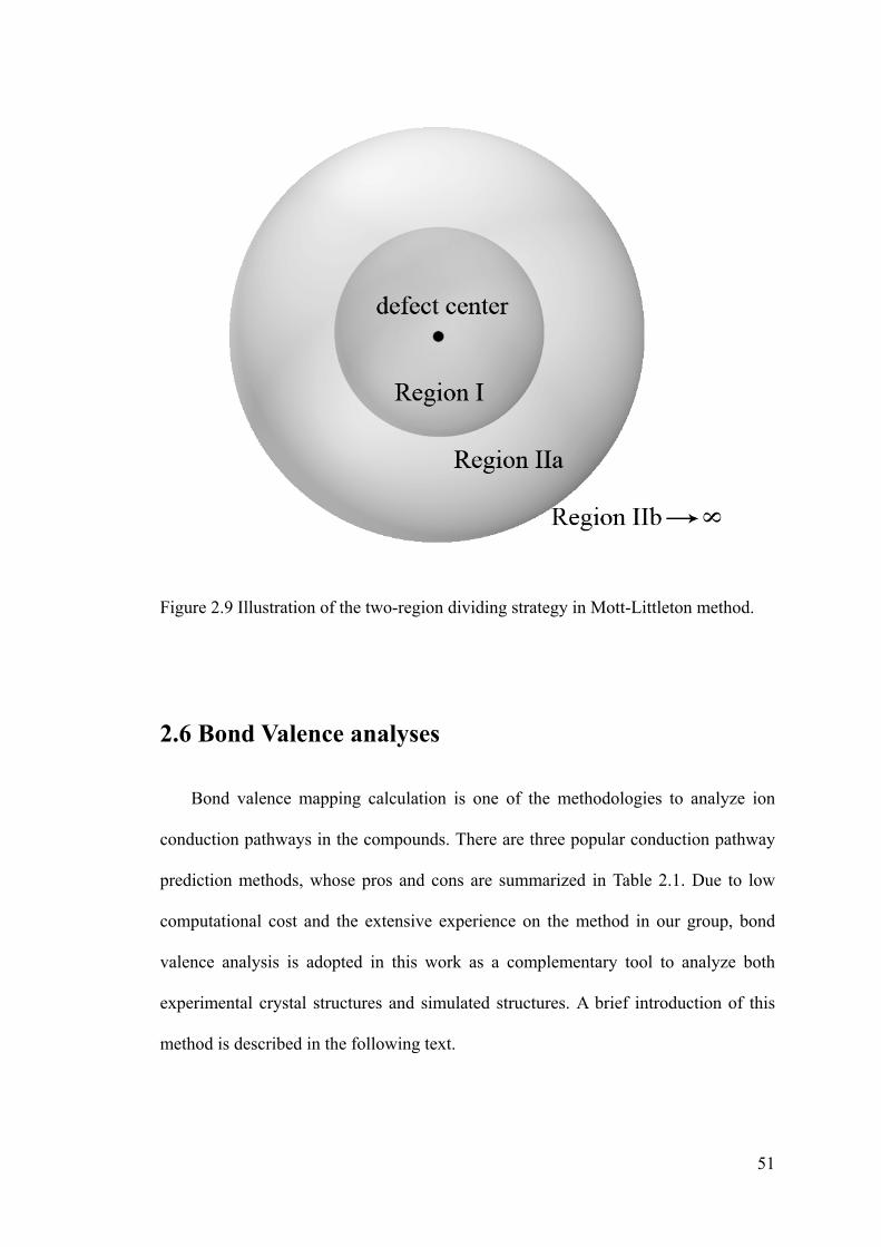
51
Figure 2.9 Illustration of the two-region dividing strategy in Mott-Littleton method.
2.6 Bond Valence analyses
Bond valence mapping calculation is one of the methodologies to analyze ion
conduction pathways in the compounds. There are three popular conduction pathway
prediction methods, whose pros and cons are summarized in Table 2.1. Due to low
computational cost and the extensive experience on the method in our group, bond
valence analysis is adopted in this work as a complementary tool to analyze both
experimental crystal structures and simulated structures. A brief introduction of this
method is described in the following text.

52
Table 2.1 Capabilities of methods for the conduction pathway analysis, reproduced from Ref. [23]
Voronoi
tessellation Bond valence mapping
Ab initio static calculations and MD
Conductors with percolation mechanism
Yes Yes Yes
Conductors with non−percolation
mechanisms No No Yes
Non−crystalline conductors
Yesa Yesa Yes
Non−ambient conditions
Yes Nob Yes
Computational cost Very low Very low High
Quantitative information
obtained
Void size, bottleneck
radii
Activation energy and conductivity (via empirical models)
Diffusion coefficient, thermal expansion
coefficientc, activation energyc
aGiven a model obtained by reverse Monte−Carlo modeling. bOnly very limited data on temperature and pressure dependence of bond valence parameters are available. cFrom a series of MD simulations for different temperatures.
Chemical bond is one of the most useful concepts to understand the structures of
compounds and their properties. In case of solid electrolytes, our interest concentrates
on the bonds in predominantly ionic solids. The interactive forces between atoms in
ionic materials are divided into an electrostatic interaction and a short-range
interaction. The first part can be described by classical electrostatic field, while the
later part is always determined empirically. The empirical bond valence concept is
developed to treat both electrostatic and short-range interactions together. The
quantity of bond valence sA-X is determined from the bond length R according to
Equation (2.12), where R0 (the length of bond corresponding to unit valence) and b
are parameters refined from sets of well-defined crystal structures (cf. [24−26]).
0exp[( ) / ]A Xs R R b (2.12)
Here, A is supposed to be a mobile ion, while X represents the immobile
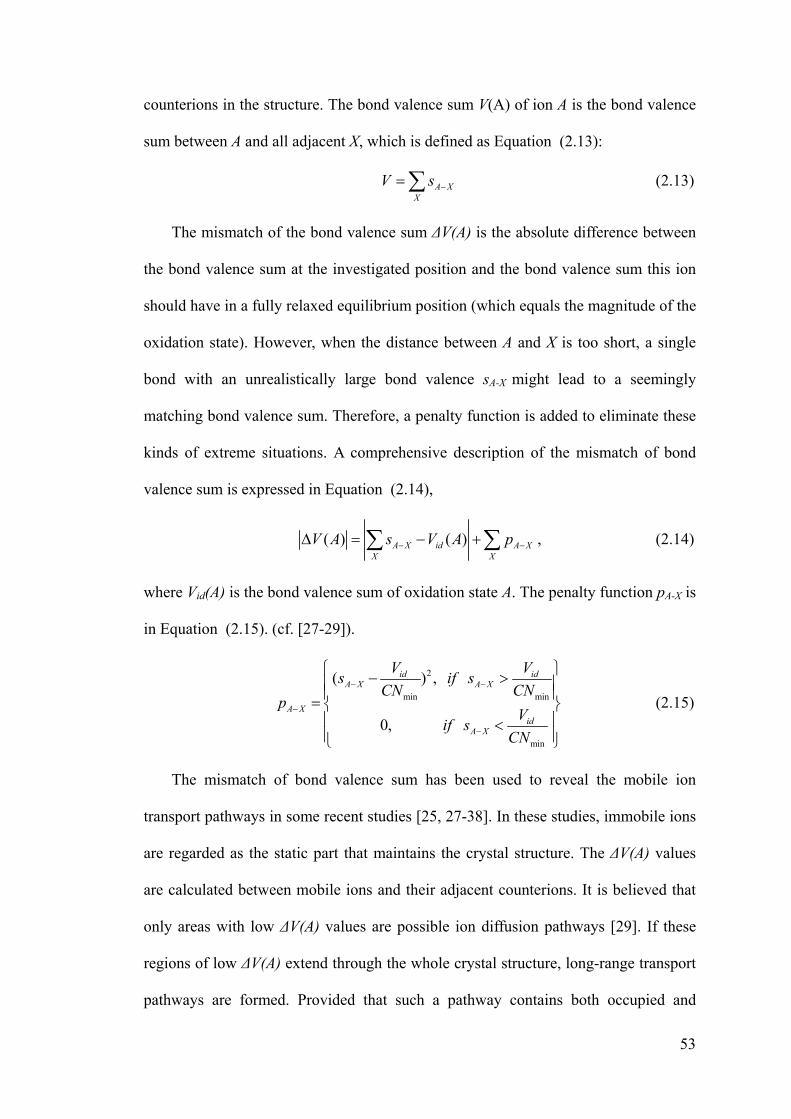
53
counterions in the structure. The bond valence sum V(A) of ion A is the bond valence
sum between A and all adjacent X, which is defined as Equation (2.13):
A XX
V s (2.13)
The mismatch of the bond valence sum ΔV(A) is the absolute difference between
the bond valence sum at the investigated position and the bond valence sum this ion
should have in a fully relaxed equilibrium position (which equals the magnitude of the
oxidation state). However, when the distance between A and X is too short, a single
bond with an unrealistically large bond valence sA-X might lead to a seemingly
matching bond valence sum. Therefore, a penalty function is added to eliminate these
kinds of extreme situations. A comprehensive description of the mismatch of bond
valence sum is expressed in Equation (2.14),
( ) ( )A X id A XX X
V A s V A p , (2.14)
where Vid(A) is the bond valence sum of oxidation state A. The penalty function pA-X is
in Equation (2.15). (cf. [27-29]).
2
min min
min
( ) ,
0,
id idA X A X
A Xid
A X
V Vs if s
CN CNp
Vif s
CN
(2.15)
The mismatch of bond valence sum has been used to reveal the mobile ion
transport pathways in some recent studies [25, 27-38]. In these studies, immobile ions
are regarded as the static part that maintains the crystal structure. The ΔV(A) values
are calculated between mobile ions and their adjacent counterions. It is believed that
only areas with low ΔV(A) values are possible ion diffusion pathways [29]. If these
regions of low ΔV(A) extend through the whole crystal structure, long-range transport
pathways are formed. Provided that such a pathway contains both occupied and

54
vacant sites for A, then it may be concluded that A is a mobile ion species in this
structure (see Figure 2.10).
Figure 2.10 Ag+ conduction pathways in α-AgI after Adams et al. [27]
The above-mentioned version of the bond valence analysis implicitly assumes
that a static structure model can reproduce the relevant features of the instantaneous
local structure. To eliminate the need for such an assumption, the evolution of ion
transport pathways in time can also be studied by bond valence method. The
BV-analysis of dynamic energy landscapes in MD trajectories will permit to identify
critical states and thereby a prediction of the kinetics of elementary steps of ion
transport and solid-state reaction steps. The fundamental advantage of such an
energy-landscape approach is that it permits the modeling of events that are too rare
(or take too long) to be observed directly in MD simulations, but are too fast to be
directly observed e.g. from classical diffraction experiments.
In this project, this dynamic bond valence analysis will be applied to molecular
dynamics trajectories. The suitability of the bond-valence analysis of dynamic energy

55
landscapes from bond valence analyses of entire trajectories will be evaluated. It is to
be expected that this would promote a better understanding of transport processes that
involve polyatomic mobile species or complex reorganizations in the immobile
sublattice as well as the description of correlations between mobile ions. As an
example of polyatomic mobile species it will be tested whether the motion of
polyatomic anions MO42− (M=W, Mo) can explain the ionic conductivity in the
Sc2(WO4)3 structure that is presently presumed to be a high-valent cation conductor.
References
[1] R. A. Young, The Rietveld Method. Oxford: Oxford University Press, 1993.
[2] H. M. Rietveld, J. Appl. Crystallogr. 2 (1969) 65.
[3] A. C. Larson, and R. B. von Dreele, Los Alamos National Laboratory Report LAUR (2000) 86.
[4] B. Toby, J. Appl. Crystallogr. 34 (2001) 210.
[5] C. A. C. Sequeira, and A. Hooper, Solid State Batteries. Dordrecht: Martinus Nijhoff Publishers, 1985.
[6] C. M. A. Brett, and M. O. Brett, Electrochemistry − Principles, Methods, and Applications. New York: Oxford University Press Inc., 1993.
[7] J. R. Macdonald, Impecance Spectroscopy − Emphasizing Solid Materials and Systems. New York: John Wiley & Sons, 1987.
[8] E. Barsoukov, and J. R. Macdonald, Impedance Spectroscopy − Theory, Experiment, and Applications. Second Edition, New Jersey: John Wiley & Sons, 2005.
[9] D. J. Driscoll, M. S. Islam, and P. R. Slater, Solid State Ionics 176 (2005) 539.
[10] J. Maier, Physical Chemistry of Ionic Materials − Ions and Electrons in Solids. John Wiley & Sons, Ltd, 2004.

56
[11] I. D. Raistrick, Annu. Rev. Mater. Sci. 16 (1986) 343.
[12] D. C. Grahame, J. Electrochem. Soc. 99 (1952) 350C.
[13] S. R. Taylor, and E. Gileadi, Corros. Sci. 51 (1995) 664.
[14] C. Tubandt, Hamb. Exp. Physi. 12 (1932) 383.
[15] F. Ercolessi, A molecular dynamics primer. Trieste: Spring College in Computational Physics, ICTP, 1997.
[16] R. P. Rao, Ph. D. thesis, Department of Physics, Indian Institute of Technology Madras (2005).
[17] L. Verlet, Phys. Rev. 159 (1967) 98.
[18] A. S. Côté, B. Smith, and P. J. D. Lindan, A Molecular Dynamics tutorial, http://www.compsoc.man.ac.uk/~lucky/Democritus/Theory/pbc−mi.html, Daresbury Laboratory (2001).
[19] A. B. Lidiard, J. Chem. Soc., Faraday Trans. 2 85 (1989) 341.
[20] N. F. Mott, and M. J. Littleton, Trans. Faraday Soc. 34 (1938) 485.
[21] C. Richard, and A. Catlow, JCS Faraday Trans. 2 85 (1989) 335.
[22] J. D. Gale, JCS Faraday Trans. 93 (1997) 629.
[23] V. V. Kharton, Solid State Electrochemistry I: Fundamentals, Materials and their Applications. Weinheim: WILEY−VCH, 2009.
[24] S. Adams, softBV web pages, http://www.softBV.net, (2007).
[25] S. Adams, Acta Crystallogr. B 57 (2001) 278.
[26] I. D. Brown, The Chemical Bond in Inorganic Chemistry − The Bond Valence Model. New York: Oxford University Press, 2002.
[27] S. Adams, and J. Maier, Solid State Ionics 105 (1998) 67.
[28] S. Adams, and J. Swenson, Phys. Rev. Lett. 84 (2000) 4144.
[29] S. Adams, Solid State Ionics 177 (2006) 1625.

57
[30] S. Adams, J. Power Sources 159 (2006) 200.
[31] S. Adams, and J. Swenson, Phys. Chem. Chem. Phys. 4 (2002) 3179.
[32] A. Hall, S. Adams, and J. Swenson, Phys. Rev. B 74 (2006).
[33] C. Müller et al., Phys. Rev. B 75 (2007) 014203.
[34] V. Thangadurai, S. Adams, and W. Weppner, Chem. Mater. 16 (2004) 2998.
[35] S. Adams, B. Mater. Sci. 29 (2006) 587.
[36] S. Adams, and J. Swenson, Phys. Rev. B 6305 (2001).
[37] S. Adams, Solid State Ionics 136 (2000) 1351.
[38] S. Adams, and J. Swenson, Solid State Ionics 154 (2002) 151.

58
Chapter 3
Chapter 3 Discovery of Polyatomic
Anion Diffusion in Solid Sc2(WO4)3
3.1 Introduction
The ion transport mechanism in A2(MO4)3 oxides with the scandium tungstate
structure, where A represents trivalent Sc3+, In3+, Al3+ or rare earth cations RE3+, and
M is usually W6+ or Mo6+, will be studied in this chapter using a combined method of
experimental and computer simulations. Experimental work, e.g. in situ powder
diffraction studies and electrochemical experiments, will provide important reference

59
information, such as the variation of the crystal structure with temperature and the
conductivity information, for comparison with the computer simulation results. In the
first stage computational studies aimed at reproducing the experimentally observed
structural features (e.g. negative thermal expansion behavior) to optimize and validate
the forcefield used in the Molecular Dynamics (MD) simulations. Then next and the
most important procedure has been to identify out the actual conducting species in
Sc2(WO4)3 type oxides by directly investigating which species can diffuse
spontaneously in the structure in MD simulations. In addition, more evidence to verify
the polyatomic anion conduction will be provided by dynamic bond valence transport
pathway analyses and Tubandt experiments.
3.2 Methods
3.2.1 Experimental
Sc2(WO4)3 sample pellets are prepared by conventional solid-state techniques,
from the mixture of stoichiometric amounts of Sc2O3 (purity 99.99%, Grirem) and
WO3 (purity 99.9%, Fluka) by repeated grinding and firing at 1000ºC. Using the
inverted crucible technique (see Chapter 2, section 2.2) the atmosphere around the
sample was saturated with WO3 to prevent an evaporation of WO3 from the sample.
The sample pellets were then characterized by in situ X-ray powder diffractometry.
Details of the measurement parameters are given in section 2.3.1. The temperature
variation at the sample position inside the oven chamber is within 2-3% of the heating
element temperature [3]. Rietveld refinements of XRD powder patterns for the wide
temperature range 11K – 1300 K are performed with the Generalized Structure
Analysis System (GSAS) by Larson and von Dreele [4], along with the graphical user

60
interface EXPGUI [5]. Structure data from published neutron diffraction
measurements by Evans et al. [1] for the low temperature range 10 – 450K were used
as the starting point of the refinement. Measurement conditions and refinement
procedures are standardized to avoid that differences in the refinement procedure
affect the observed temperature dependence of structural details. All structures at
different temperatures are thus refined based on the same set of 52 refinable
parameters: 12 background variables of a shifted Chebyschev function, 7 profile
variables, 3 cell parameters, 25 refinable atomic coordinates, 3 atomic displacement
parameters, 1 preferential orientation parameter and an overall scale factor.
Impedance spectra are recorded with a Solartron SI 1260 impedance analyzer, using
sintered pellets with sputtered platinum electrodes as ion blocking electrode on both
sides. Measurements were carried out over frequency range from 1Hz to 1MHz in the
temperature range from 550K to 1300K in steps of 25K.
For each Tubandt measurement [6] three disks of Sc2(WO4)3 ceramics with
polished surfaces were inserted between Pt electrodes. The typical thickness of an
individual disk was 1.4 mm. A voltage of 300 V was applied for 21−48 hrs at a
temperature in the range 940 – 990 ºC. Currents were limited to 1mA but in most
cases average currents were only about 0.1 mA owing to the low conductivity of
Sc2(WO4)3 disks at the chosen temperature. The relative porosity of the samples did
not exceed 0.2. Gorelov’s modified EMF technique [7] (which uses an external active
load to minimize the effect of electrode polarization) was used to redetermine the
ionic transference number.

61
3.2.2 Computer simulations
Molecular dynamics simulations for a 1224 atom (3a × 2b × 3c ) supercell were
performed using the Cerius2 (for isothermal-isobaric, NPT) and Materials Studio (for
isothermal-isochoric, NVT) software suites by Accelrys [8, 9], using the same
parameters based on a modified UFF universal forcefield as discussed in section
3.3.2.1 [10]. Integration of the equation of motion has been performed with a Verlet
velocity algorithm [11] in Materials Studio or a Verlet leapfrog algorithm in Cerius2.
Time steps have been chosen as 1.5 fs for the evaluation of the diffusion coefficients
or 1.0 fs for the transport mechanism investigation. Coulombic interactions have been
calculated by the Ewald summation method with a cutoff of 12.5 Å and an accuracy
of 0.001 kcal/mol and a short range interaction cutoff of 5.61 Å. Temperature is
controlled using the Nosé-Hoover thermostat and pressure (for the case of the NPT
simulations) by the Parrinello-Rahman barostat (Cell mass prefactor =10). For the
assessment of diffusion coefficients NVT simulations are run for 8.5 ns (for T = 1350
K) to 13.5 ns (for T=1200K).
Diffusion pathways were studied by bond valence analysis, the theory of which is
described in section 2.6. Specially refined parameter values for the Sc3+ − WO42−
interaction (R0= 3.39949 Å, b = 0.5Å, cut−off radius: 7 Å) [12] are used to test the
mobility of WO42− ions, treating it as a pseudoatom.

62
3.3 Results and discussion
3.3.1 Non-ambient XRD and structure refinement
Results of the Rietveld refinements for the structure of Sc2(WO4)3 are
summarized in Table 3.1. Atomic fractional coordinates of the Sc2(WO4)3 structure at
each investigated temperature from 11K to 1300K are listed in Table A.1. As an
example Figure 3.1 shows the refinement for 300K data (measured in the heating
chamber). More refinement results and XRD profiles are shown in Figure A.1 and
Figure A.2. Cell parameters of heating and cooling cycle agree. Using the heating
cycle data listed in Table 3.1 as a calibration curve, temperatures of the cooling cycle
data can be determined from the lattice constants with an accuracy of ±20K. From the
temperature variation of the lattice constants plotted in Figure 3.2, it can be seen that
there is a minute offset between our results obtained in high and low temperature
diffraction setups, but the trend is identical. The thermal expansion coefficients
derived from these measurements are given in Table 3.2. For the lower temperature
range the values are in reasonable agreement to those found by Evans et al. [1], while
earlier single crystal dilatometric data by Balashov et al.[13] are inconsistent with our
or Evans’ findings. For the high temperature range, where no diffractometric reference
data existed, we find a reduction of the magnitude of all linear expansion coefficients.

63
Table 3.1 Cell Dimensions as a Function of Temperature
T (K) a (Å) b (Å) c (Å) V (Å3) Rwp(%)b R(F2)(%)
11a 9.68300(11) 13.31784(15)9.59151(11)1236.889(31) 6.76 4.12
50a 9.68301(11) 13.31962(15)9.59143(11)1237.045(30) 7.51 4.24
100a 9.68232(12) 13.32028(17)9.59088(12)1236.947(33) 6.87 3.84
150a 9.68078(7) 13.32122(10) 9.58941(7) 1236.650(20) 7.24 3.94
200a 9.67845(8) 13.32378(11) 9.58721(8) 1236.305(22) 7.86 4.46
250a 9.67514(7) 13.32701(9) 9.58449(7) 1235.830(18) 7.43 4.12
300c 9.67132(9) 13.33083(13) 9.58179(9) 1235.341(25) 6.95 3.88
300d 9.67144(7) 13.32617(9) 9.58110(7) 1234.842(17) 5.96 4.16
350 9.66691(6) 13.33105(8) 9.57804(6) 1234.314(16) 5.94 4.49
400 9.66276(6) 13.33496(8) 9.57504(6) 1233.769(15) 5.91 4.52
450 9.65894(6) 13.33824(8) 9.57242(6) 1233.247(15) 6.04 4.70
500 9.65542(5) 13.34124(7) 9.57000(5) 1232.762(14) 5.88 4.90
550 9.65206(5) 13.34383(7) 9.56777(5) 1232.273(13) 5.78 5.10
600 9.64871(5) 13.34598(7) 9.56563(5) 1231.781(13) 5.87 5.44
650 9.64531(5) 13.34780(7) 9.56346(5) 1231.235(13) 6.04 5.71
700 9.64246(5) 13.34917(7) 9.56139(5) 1230.718(13) 5.92 6.01
750 9.63955(5) 13.35026(7) 9.55959(5) 1230.241(13) 6.00 6.20
800 9.63696(5) 13.35110(7) 9.55783(5) 1229.748(13) 6.03 6.33
850 9.63440(5) 13.35201(7) 9.55607(5) 1229.280(13) 6.16 6.63
900 9.63194(5) 13.35293(7) 9.55447(5) 1228.844(13) 6.13 6.85
950 9.62970(5) 13.35375(7) 9.55309(5) 1228.457(13) 6.16 6.83
1000 9.62760(5) 13.35461(7) 9.55164(5) 1228.081(13) 6.25 6.96
1050 9.62547(5) 13.35535(8) 9.55038(5) 1227.725(14) 6.21 7.15
1100 9.62355(6) 13.35626(8) 9.54910(6) 1227.390(14) 6.22 7.38
1150 9.62166(6) 13.35709(8) 9.54792(6) 1227.073(14) 6.04 7.28
1200 9.61988(6) 13.35768(8) 9.54671(6) 1226.746(15) 5.96 7.65
1250 9.61797(6) 13.35797(8) 9.54552(6) 1226.376(15) 5.93 7.91
1300 9.61588(6) 13.35786(9) 9.54392(6) 1225.894(17) 6.06 8.02 aRefined from 3 sets of XRD diffraction data bweighted profile R-factor after background subtraction. cmeasured in cryostat. dmeasured in high temperature chamber.

64
Table 3.2 Linear thermal expansion coefficients for lattice constants a – c and expansion coefficient of the unit cell volume V
This worka,c (10−6·K−1) Evansa (10−6·K−1) Balashovb (10−6·K−1)
100−700K 700−1300K 50−450K 293−873K
a −7.37 −4.3 −6.49 −5.45
b 3.97 1.09 5.61 4.43
c −5.41 −2.82 −5.73 −1.6
V −8.8 −6.02 −6.44 not reported
a from powder diffraction; b from single crystal dilatometry; c Two linear regions are observed in this work: one is 100−700K, the other one is 700−1300K, while data for T< 100K deviate therefrom.
Figure 3.1 Refinement of Sc2(WO4)3 structure at 300K with final Rwp=5.96%. Observed (×), calculated (line), and Observed − calculated (lower line). The inset shows the details of the refinement result in the 2 theta range from 18° to 31°.

65
Figure 3.2 Temperature dependence of (a) unit cell parameters and (b) cell volume of Sc2(WO4)3 as determined from high temperature (▲) or low temperature (■) XRD data in this work. Neutron diffraction data by Evans [1] (○) are shown for comparison.
0 200 400 600 800 1000 1200 14009.54
9.56
9.58
9.60
9.62
9.64
9.66
9.68
9.70
13.20
13.25
13.30
13.35
13.40
Cel
l dim
ensi
on
/ Å
Temperature / K
(a)
c-axis
b-axis
a-axis
0 200 400 600 800 1000 1200 1400
1226
1228
1230
1232
1234
1236
1238
(b)
Cel
l Vo
lum
e / Å
3
Temperature / K

66
Beyond the variation of the unit cell, the variation in the freely Rietveld refined
atomic coordinates provides further insight into the local mobility of the building
blocks of the Sc2(WO4)3 structure. For such an open framework structure that permits
large angle rotations of nearly rigid building blocks, the apparent distance between the
average positions of two bonded atoms that is observed in an XRD structure
determination does not match the “true” average instantaneous distance. (For a more
detailed discussion see e.g. [1]). In brief, a negative thermal expansion can be
expected if such correlated rotations dominate over uncorrelated vibrations of the
individual atoms, which via the anharmonicity of the interaction potential are the
source of the normal thermal expansion. A high correlation of the rotations can be
expected if the interatomic interactions are both strong and directional. In Figure 3.3
(a) this apparent average bond length is plotted as a function of temperature. When T
increases, the Sc-O bond length increases, while W-O bond appears to become shorter.
This apparent displacement of the O towards the W is a consequence of the increase
in the amplitude of the O atom vibration perpendicular to the bond axis. The finding
that this results in an apparent shortening of the bond only for W-O bonds, but not for
Sc-O bonds, suggests that the motion of the O is more effectively controlled by the
nearby W. To a good approximation the polyatomic anion WO42− may be regarded as
a rigid unit (while the ScO6 coordination polyhedron is significantly less rigid).
Therefore, we expect that the energy to break the more ionic Sc-O interaction should
be significantly lower than the energy to break the more covalent W-O bond.

67
Figure 3.3 Temperature dependence of (a) the average apparent bond length and (b) of the atomic displacement parameters in Sc2(WO4)3 as determined from Rietveld refinements.

68
For the sake of refinement stability we have limited the direct evaluation of
thermal displacement from the Rietveld refinement to one isotropic atomic
displacement parameter per atom type. Still the analysis of the refined values of Uiso
displayed in Figure 3.3 (b) gives some indications on the differences between the
local mobilities of the various potential charge carriers. As expected, the highest Uiso
at each temperature is observed for the oxygen atoms, both because oxygen is the
lightest atom and because the apparent Uiso includes contributions from the rotation of
the rigid polyatomic unit that might cause the saturation tendency at elevated
temperatures. It should be noted that in the high temperature range the value of Uiso
for W6+ is larger than the one of the (significantly lighter) Sc3+ ion, which points
towards an unusually high local mobility of the W atom, including but not necessary
limited to the rotation of the WO4 units.
3.3.2 Computational and experimental studies of the dynamic
structure
3.3.2.1 Modification of forcefield to reproduce volume and NTE
In this work MD simulations are employed both directly to analyze diffusion
coefficients and thereby the ionic conductivities of mobile charge carriers and as a
basis for a dynamic ion transport pathway analysis. To ensure that the forcefield
parameters are realistic, we first tried to reproduce not only the lattice constants, but
also the characteristic negative thermal expansion behaviour by NPT simulations.
The structure of Sc2(WO4)3, as shown in Figure 1.5, is usually regarded as being a
three-dimensional framework built up by WO4 tetrahedra that are corner-linked to

69
ScO6 octahedra. As sketched in Figure 3.4, the observed reduction of the apparent
W-O distances is due to large amplitude librations of the building blocks that directly
translate into a reduced Sc-W distance and thus into a negative thermal expansion in
the W-Sc direction (cf. Evans [1]). The standard universal forcefield (UFF) [10] as
implemented in Cerius2 in combination with QEq [14] charges clearly fails to
reproduce the experimental volume or the negative thermal expansion behavior (room
temperature unit cell volume VRT: 1234.8 Å3 (experimental), 1951.3 Å3 (UFF) volume
expansion coefficients for 100K < T < 700K: α = −8.8×10⁻⁶ K−1 (experimental),
+14.1×10⁻⁶ K−1 (UFF)). To this end we revised the Sc-O interaction in the UFF,
replacing original Lennard Jones-type nonbonded interactions by the more realistic,
yet computationally more expensive Morse potential (see Equation (3.1)).
0
( 1)2 2
0( ) ((1 ) 1)y r
rV r D e
, where 0 02 / 2y r k D (3.1)
with the parameters bond energy D0, equilibrium bond distance r0, and potential width
exponent y, which depends on r0, D0 and the bond force constant k, while the
calculation of fractional charges for the Coulomb interactions by means of the QEq
formalism remain unchanged. The chosen form of the interaction potential V(r) has to
allow that Sc−O bonds can be broken with a finite activation energy, since any of the
considered ion transport mechanisms would require the breaking of a Sc3+−O bond.
Thereby even if the accuracy of the chosen parameters is difficult to prove, it should
only have a minor influence on whether Sc3+ or WO42− is the most mobile species. In
this work we use the parameters D0(Sc−O)=2 kcal / mol, r0 (Sc−O)= 2.4 Å and y = 11
as simulations using these values come closest to a reproduction of the unit cell
volume and thermal expansion behavior. With these parameters and QEq charges the
breaking of a Sc-O bond requires a dissociation energy of 90.6 kcal/mol, and for
equilibrium distances the bond energy is dominated by the Coulomb interaction. For

70
W−O bonds we assumed a simple harmonic bond stretching term (spring constant k0
= 600 kcal / (molÅ2), r0 = 1.75 Å), so that the simulation cannot yield any predictions
on mechanisms involving the breaking of W−O bonds. As discussed already in
section 1.2.2, conduction by free oxide ions is anyway highly unlikely due to the
insensitivity of the ionic conductivity to the oxygen partial pressure. For 300K the
simulation yields a cell volume of 1233.1 Å3 closely matching the experimental unit
cell volume of 1234.8 Å3. The negative thermal expansion along the a and c direction
(and positive expansion along the b direction) is reproduced in our MD simulations
over a limited temperature range, though the expansion coefficient α = −2.0×10⁻⁶·K−1
averaged over the temperature range 100K < T < 700K is still underestimated by the
revised forcefield. The variation of the simulated lattice constants is plotted in Figure
3.5.
Figure 3.4 Schematic representation of how the negative thermal expansion can be linked to the increase in amplitude of a rocking mode of nearly rigid building blocks. Top: dark WO4 tetrahedron, bottom light grey ScO6 octahedron; O shown as spheres. The average W – Sc distance (dotted line) drops from 3.776 Å at 50K to 3.758 Å at 1000K.

71
Figure 3.5 Variation of lattice constants a (squares), c (triangles) and b (circles) of Sc2(WO4)3 as a function of temperature in a NPT simulation (solid) which are compared with experimental data (hollow) from this work.

72
3.3.2.2 Further verification of the forcefield by reproducing the phase
transition under pressure
The validity of our forcefield used for molecular dynamics simulations is further
verified by reproducing the Sc2(WO4)3 structural orthorhombic to monoclinic phase
transition under pressure. As an example Figure 3.6 shows how the monoclinic angle
α transforms under a pressure of 0.9 GPa. The simulation starts from the
orthorhombic phase with = 90. After about 100 ps, the phase transition occurs
when the α angle tilts to about 89.5. As the system is still close to the phase transition,
the α fluctuates and later during the same simulation flipped to about 90.5. The tilted
cell we mentioned above is not the conventional cell for the monoclinic phase, but a
pseudo-orthorhombic supercell that permits a direct comparison to the orthorhombic
cell constants. The matrix to convert a conventional monoclinic cell to pseudo
orthorhombic cell is (0 1 0; 2 0 1; 0 0 −1), which will lead to an angle α > 90.
Thus the experimentally known phase transition can be successfully reproduced
in MD simulations with our forcefield. The fact that the simulated phase transition
pressure (0.8 GPa) is higher than the experimental value (0.3 GPa according to Varga
et al. [2], 0.6±0.4 GPa according to N.Grag et al. [15]), may be attributed to the
relatively short time scale and the slow kinetics of these pressure-dependent
simulations at room temperature.

73
As demonstrated in Figure 3.7, experimental and simulated lattice constants and
the angle α vary qualitatively similar with increasing pressure. Though the transition
pressure is different, the variation of the simulated monoclinic lattice constants is in
good agreement with the extrapolation of the experimental values by Varga.
(Experimental data are so far only available up to 0.61 GPa).
Figure 3.6 Variation of the angle α with time in an isothermal−isobaric (NPT) simulation for the pressure p = 0.9 GPa.
0 100 200 300 400 50088.5
89.0
89.5
90.0
90.5
91.0
91.5
/ d
eg
Time / ps
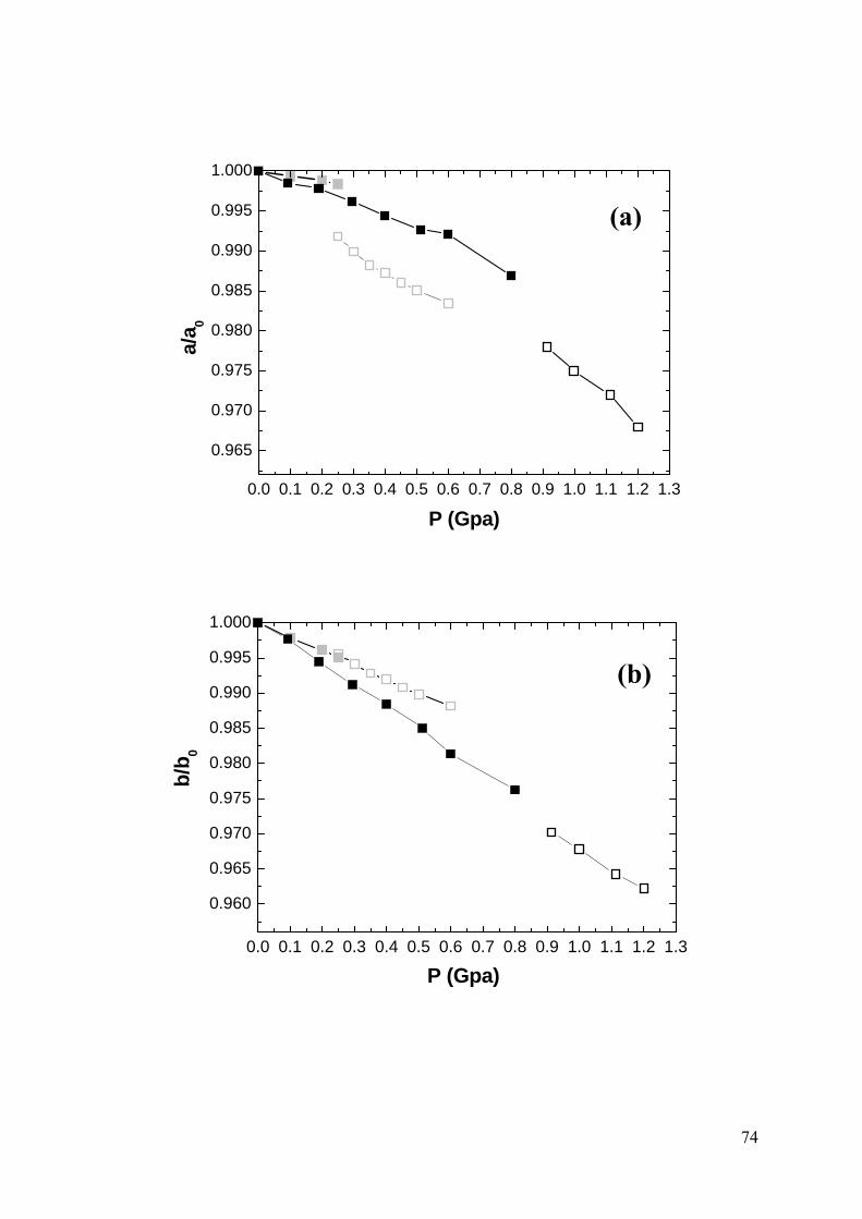
74
0.0 0.1 0.2 0.3 0.4 0.5 0.6 0.7 0.8 0.9 1.0 1.1 1.2 1.3
0.965
0.970
0.975
0.980
0.985
0.990
0.995
1.000
(a)a/
a 0
P (Gpa)
0.0 0.1 0.2 0.3 0.4 0.5 0.6 0.7 0.8 0.9 1.0 1.1 1.2 1.3
0.960
0.965
0.970
0.975
0.980
0.985
0.990
0.995
1.000
(b)
b/b
0
P (Gpa)

75
Figure 3.7 Comparison of simulated lattice constants and monoclinic angle α as a function of pressure with experimental literature values [2]: (a), (b) and (c) normalized lattice constants. (d) monoclinic angle α. For all pressures the (pseudo-) orthorhombic setting has been chosen to emphasise the structural relationship of the high and low pressure phases. Experimental values: grey symbols; simulated values: black symbols. The low pressure orthorhombic phase is marked by filled squares and the high pressure monoclinic phase by open squares.
0.0 0.1 0.2 0.3 0.4 0.5 0.6 0.7 0.8 0.9 1.0 1.1 1.2 1.3
0.960
0.965
0.970
0.975
0.980
0.985
0.990
0.995
1.000
(c)c/
c 0
P (Gpa)
0.0 0.1 0.2 0.3 0.4 0.5 0.6 0.7 0.8 0.9 1.0 1.1 1.2 1.3
89.4
89.5
89.6
89.7
89.8
89.9
90.0
(d)
(deg
)
P (Gpa)
76
3.3.2.3 Conductivity
With this modified forcefield, NVT simulations were performed for 4
temperatures in the range 1200K − 1350K for the equilibrated lattice constants at each
temperature. The simulated periods ranged from 8.5 ns for T=1350K to 13.5 ns for
T=1200K. For the simulations at T=1300K and 1350K hops of WO42− groups are
observed, while none of the simulations indicated local hops of Sc3+ ions. (As
mentioned above we cannot expect O2− hops due to the choice of the forcefield). A
more detailed analysis of the MD simulation trajectory reveals that several hops are
highly correlated. This can be visualized by plotting the trace of the moving WO42−
group. Figure 3.8 (a), produced with gOpenMol [16], shows traces for the motion of
W atoms (the centers of the WO42− group). In Figure 3.8 (a) nine WO4
2− groups
formed a pathway through the supercell. Thereafter the initial defect vanishes again
when the 9th WO42− fills the translation copy of the vacancy created in the initial step.
The traces for Sc atoms are also shown in Figure 3.8 (b), illustrating that the
simulated Sc atoms just oscillate around their equilibrium positions and do not exhibit
any tendency to leave these sites. Thus according to the MD simulations obviously
WO42− and not Sc3+ is the diffusing charge carrier in Sc2(WO4)3.
A detailed “rock and roll” transport mechanism is shown in Figure 3.9. One
WO42− group pushes its adjacent WO4
2− group into an interstitial site and fills in the
vacancy. The translational motion of WO42− group can be understood as a transition
from the large amplitude rocking of the WO42− group to a rolling into a new average
position (cf. section 3.3.2.3 below).

77
Figure 3.8 The trace of the motion of (a) W atoms (initial positions of the nine moving WO4
2− groups indicated as circles; the first hop from an equilibrium site to an interstitial tungstate site is marked by an arrow) and (b) Sc atoms for the NVT simulation of Sc2(WO4)3 at T=1300K.

78
Figure 3.9 “Rock and roll” transport mechanism for tungstate ions in Sc2(WO4)3. Graphs (a) - (f) show an elementary transport process from details of snapshots from 5 ps of a 5 ns MD simulation (T =1300 K). The direction of motion is highlighted by arrows. A regular WO4
2− ion A (shown as ball and stick) reorients under the influence of an approaching interstitial WO4
2− ion B (shown as grey tetrahedron), (a) and then rolls to an interstitial position (b, c). After a further reorientation step (d) ion B fills the site previously occupied by A (e, f).
(a) (d)
(b) (e)
(c) (f)

79
As mentioned above, for the simulations of ordered Sc2(WO4)3 described so far,
hops of WO42− are observed for the higher simulated temperatures 1300K and 1350K
only. From these hops the time dependence of the mean squared displacement (MSD,
see Figure 3.10 (a)) for WO42− and (therefore via the Nernst-Einstein equation) the
conductivity is roughly assessed. Simulated and experimental conductivity data are
plotted in Figure 3.10 (b), along with experimental data from the literature [17, 18].
Data by Driscoll for the limited temperature range 625-960K are consistent with our
findings, while values reported by Imanaka are somewhat larger. Differences might be
partially related to differences in the density of the samples. When comparing
experimental and simulated conductivities, it should be noted that – as discussed
further below − the obtained absolute conductivity values will substantially depend on
defect creation steps that occur only rarely even for the rather long simulated periods
as well as on the length of the chain of migration steps before the defect vanishes
(which may be affected by the size of the chosen supercell). Thereby the observed
good agreement with both our own and literature data on the experimental
conductivity should be taken with care.
The inset in Figure 3.10 (b) emphasizes the variation of the experimental
activation energy. We find a plateau of the activation energy of 65 kJ/mol for T<800K,
then a gradual decrease to a value of ca. 45 kJ/mol for 1100−1200 K and a slight
increase for the highest temperature range (1200−1300K). While the range of
observed activation energies is similar for the literature data, the temperature where
the decrease in activation energy sets in varies significantly.

80
Figure 3.10 (a) Simulated mean square displacement of WO42− and Sc3+ vs. time for a
NVT simulation of Sc2(WO4)3 at T = 1300K. (b) Comparison of simulated conductivity (■), experimental conductivities obtained in this work (□). Experimental data by Driscoll et al. [17] (●) and by Imanaka et al. [18] (▲) are shown for comparison. The inset graph shows the variation of the activation energy with temperature as derived from the three sets of experimental conductivity data (using the same symbols).
2

81
3.3.2.3 Analysis of WO42− rotation and transport mechanism
As the hopping of the relatively large WO42− in the solid state has so far not been
observed, we tried to analyze the mechanism of the polyatomic anions in this novel
type of solid electrolytes more in detail. We noted that the hopping of WO42− group is
inevitably accompanied by a rotation of the tetrahedron. In Figure 3.11 the diffusion
of the WO42− group is tracked by the variation of the distance of the central W from
its position in the reference frame. The time steps of elementary diffusion steps are
then compared to time steps where rotations of the WO42− group occur. The
tetrahedron rotations are registered as changes in the orientation of W-O bonds, which
is simply expressed by the angle between the bonds and the x axis. Orientation angles
are traced for two different W-O bonds to capture all rotations. It is found that all
elementary hopping steps, such as the ones that can be seen in Figure 3.11 at t = 3404
ps and 3426 ps, are accompanied by reorientations, so that one might rather describe
the elementary transport step as a rolling of the WO42− group to its new position. On
the other hand some further rotations shown in Figure 3.11, such as the one at t =
3450 ps, are not connected to translational diffusion steps. Based on the selected
range of frames in Figure 3.11 it is also noted that the values and fluctuations of the
W-O bond length (1.698 ± 0.072 Å) or O-W-O bond angles (106º ± 10º) around the
time steps of the hopping processes exceed the normal fluctuations (1.699 ± 0.067 Å,
109º ± 7º) only slightly, supporting the model of WO42− being a rather rigid building
block.

82
Figure 3.11 Correlation between the variation of the distance of a WO42− (with respect
to its position at t0 = 3400 ps) and the change in the orientation angle of two W-O bonds (with respect to the x axis) over 69 ps with a resolution of 0.1ps.
It may be noted that the finding of anion rotation in solid electrolytes as such is
not new. The motion of monovalent cations under the influence of rotation of anions
such as SO42− and PO4
3− has been the subject of long-standing discussions (see
e.g.[19−21]), but the proposed transport mechanism for Sc2(WO4)3 obviously differs
from such rotator phases and the proposed “paddle-wheel mechanism” [21] in that the
tungstate anion in Sc2(WO4)3 is the mobile species, rather than the facilitator for a
cation motion.

83
3.3.2.4 Bond valence analyses of long range transport in Sc2(WO4)3
Bond valence analyses for the geometry optimized structure of Sc2(WO4)3 have
been performed in our previous work and will only be briefly summarized here [12].
Bond valence maps of Sc3+ and O2− show that only isolated regions of low bond
valence mismatch value exist for these two ions. In the case of O2− these regions again
indicate that the lowest energy local motion should correspond to the collective
rotation of the entire tungstate ion. When we however analyze the BVS mismatch
for WO42− (treating it as a pseudo-atom), extended regions of low bond valence sum
mismatch are observed that link occupied and unoccupied tungstate sites thereby
forming pathways for a long range diffusion of WO42−. Still it should be kept in mind
that these preliminary calculations are based on static average structure models and
that treating tungstate as a pseudo-atom may not capture essential details of critical
configurations, especially for the motion of a polyatomic deformable species that as
we have seen undergoes reorientations during the hopping.

84

85
Figure 3.12 Four selected frames from a dynamic bond valence analysis with nine moving WO4
2− groups (marked by grey spheres) forming a pathway through the supercell (total time interval between frames (a) t = 3403.3ps and (d) t = 3404.5ps is 1.2 ps). The grey isosurface represents a BVS model of the instantaneous WO4
2− pathways (i.e. regions of BVS mismatch |V| < 0.25 valence units for WO4
2−). Traces of the W atoms that hop within a 69 ps period of the MD simulation (same period as for Figure 3.11) are superimposed on this BVS pathway landscape. Arrows mark the position of the first moving ion during the defect creation process. In contrast to the series of subsequent hops it does not follow the low energy transport pathway.
Thus a more detailed dynamic bond valence analysis was performed in this
project by calculating bond valence models of the instantaneous ion transport
pathways for series of time frames from the MD simulation trajectory. For each time
step the respective pathway model was constructed from the instantaneous atomic
positions of the MD trajectory. Figure 3.12 monitors the evolution of BV ion transport
pathways for a series of time steps from such a dynamic ion transport pathway model.

86
As shown in Figure 3.12 characteristic features of the ion transport pathways remain
stable over periods exceeding the time scale of local hopping processes, though there
is substantial fluctuation of the regions accessible at every instant. As had been found
previously for other ion conductors [22], ion transport pathways remain limited to a
small portion of the total volume. Once a defect has been formed, ion transport clearly
follows this fluctuating network of instantaneous pathways, underlining the predictive
power of the bond valence method. There is however consistently an exception at the
beginning of the chain of correlated local hopping processes: the generation of an
anti-Frenkel defect, which requires a high activation energy (cf. section 4.3.1). Even
in the fully stoichiometric ensemble such local hops of tungstate groups to nearby
interstitial sites are possible, but from these interstitial sites (discernible in Figure 3.8
(a) as sites with short residence times next to the zig-zag line of equilibrium sites) the
most probable subsequent step is the hopping back to the equilibrium site.
In the cases studied more in detail, long range transport was initiated only when a
tungstate ion with a high activation energy (i.e. capable of leaving the low BV
mismatch region) approached another tungstate ion that just left its equilibrium site to
one of the nearby low energy interstitial sites and pushes it away along the BV
pathway towards the next equilibrium site. This interstitialcy-like transport
mechanism is then repeated several times within a short period until the last
interstitial ion again finds a vacancy (in the simulations there was always just one
vacancy present and the chain of transport steps either formed a loop or led to the
vacancy in a translation copy of the original simulation cell. Thus a typical transport
event would involve one step that does not follow the bond valence pathway, such as
the one marked by arrows in Figure 3.12 starting a series of correlated ion hops along
the bond valence pathway.

87
It should be reemphasized that the tungstate Frenkel defect creation is obviously a
rare high energy process. The actually observed activation energy will depend on the
ratio between the high energy defect creation and the chain of lower energy tungstate
rearrangements made possible by the defect creation. With the limited size of the
model (1224 atoms, which was enforced by the need to run the simulations over
several nanoseconds) it is difficult to judge, whether the observed density of
vacancies and thereby the number of low-energy charge transport steps between
defect creation and annihilation is realistic. Thus it cannot be ruled out that the
reasonably good agreement between the simulated and experimental conductivities
might be to some extent a coincidence. Ongoing MD simulations with artificially
created vacancies in the supercell may help to clarify whether the variation of the
experimentally observed conductivity values for samples from different groups may
be due to a different defect concentration in these materials.
3.3 Mass and charge transfer experiments in
Tubandt-type cells with Sc2(WO4)3
EMF experiments at 940−990ºC with active loads (Gorelov’s method [7, 23])
confirm that Sc2(WO4)3 is a purely ionic conductor with an ionic transference number
1.00, while earlier literature reported t > 0.92 (based on measurements without
active loads) [24]. In the literature, the results of electrolysis experiments using a
single solid electrolyte disk in a (Pt)| A2(WO4)3|(Pt) cells have been used as evidence
of trivalent-cation conduction. However, the chemical and phase composition of
cathode and anode regions after electrolysis would be identical, independent of

88
whether Sc3+ or WO42− are the main ionic carriers. For Sc2(WO4)3, one expects the
formation of Sc6WO12 at the Sc2(WO4)3|Pt(−) boundary and WO3 at the
Sc2(WO4)3|Pt(+) boundary, regardless of the carrier.
The setup for the Tubandt-type experiment, shown in Figure 3.13 consists of
three Sc2(WO4)3 ceramic disks between two platinum electrodes:
(−)Pt│(−)Sc2(WO4)3│Sc2(WO4)3│(+)Sc2(WO4)3│Pt(+) (3.2)
If Sc3+ ions are mobile, they will migrate from the positively charged side toward
the negatively charged side according to
(+) Sc2(WO4)3 →16Sc3+ +24WO3 +12O2 + 48е− (3.3)
(−) Sc2(WO4)3 + 16Sc3+ +12O2 + 48e− → 3 Sc6WO12 (3.4)
This should decrease the mass of the (+)Sc2(WO4)3 disk and increase the mass of
the (−)Sc2(WO4)3 disk. On the other hand, if the WO42− ion is the main ionic carrier, it
will migrate from the negatively charged side toward the positively charged side,
according to:
(−) 3Sc2(WO4)3 +16e− +4O2 → Sc6WO12 + 8 WO42− (3.5)
(+) 8WO42− → 8WO3
+4O2 +16e−, (3.6)
which should result in a decrease in the mass of the (−)Sc2(WO4)3 disk and an
increase in the mass of the (+)Sc2(WO4)3 disk with the deposition of WO3.

89
Figure 3.13 Schematic setup of Tubandt-type cell experiments with stacks of 3 Sc2(WO4)3 disks for T = 940°C . Average mass changes and their standard deviations are indicated for the individual disks as observed in the four experiments listed in Table 3.3.
Table 3.3 Mass changes for 4 Tubandt experiments
№ of exp. Δm(−) (mg) Δm(+) (mg) Q (C)a Δm(−)/Q (mg/C)
Δm(+)/Q (mg/C)
I −6.1 6.0 15 −0.41 0.40 II −32.2 21.1 88 −0.37 0.24 III −3.4 0.3 18 −0.19 0.02 IV −3.4 1.1 10 −0.34 0.11
aQ: passed charge in Coulombs; Initial thickness of individual disks 1.4±0.1mm in all listed experiments.
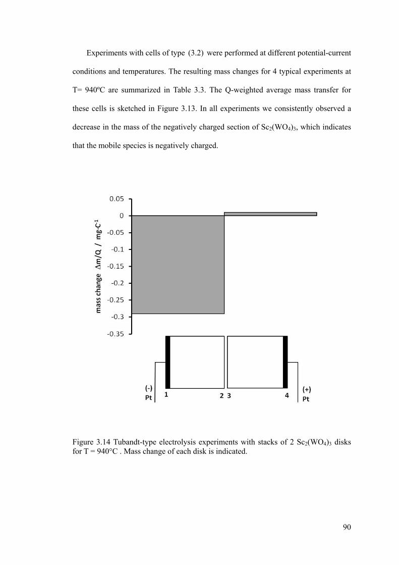
90
Experiments with cells of type (3.2) were performed at different potential-current
conditions and temperatures. The resulting mass changes for 4 typical experiments at
T= 940ºC are summarized in Table 3.3. The Q-weighted average mass transfer for
these cells is sketched in Figure 3.13. In all experiments we consistently observed a
decrease in the mass of the negatively charged section of Sc2(WO4)3, which indicates
that the mobile species is negatively charged.
Figure 3.14 Tubandt-type electrolysis experiments with stacks of 2 Sc2(WO4)3 disks for T = 940°C . Mass change of each disk is indicated.

91
Figure 3.15 Low angle XRD profile for (a): boundary (1) and (b): boundary (4) as shown in Figure 3.14. Diffraction peaks corresponding to Sc6WO12 and WO3 phases are indicated on the graphs.
12 13 14 15 16 17 18 19 20 21 22 23 24 25 260
200
400
600(a)
* Sc6WO
12
* **
Inte
nsi
ty /
a.u
.
2 theta (o)
18 19 20 21 22 23 24 25 26 27 28 29 30 310
200
400
600
800
1000
1200 (b)
* WO3
***
Inte
nsi
ty /
a.u
.
2 theta (o)

92
Since it is technically difficult to separate Pt paste electrode and the electrolyte
without destroying the electrolysis product at the interface, we performed another
Tubandt experiment with no Pt paste but contact the Pt foil electrode to the disk
surface directly. The setup and result of this experiment is shown in Figure 3.14. The
quantity of the products formed on the electrodes or in near-electrodes regions was
too low for conclusive determination by XRD or microprobe (15 Coulombs ≈
1.510−4 F), but the low angle XRD investigation of the sample surfaces suggests that
Sc6WO12 is formed for boundary (1) of Figure 3.14 (see Figure 3.15 (a)) and WO3 at
boundary (4) (Figure 3.15 (b)), which also changed its color to WO3-like.
The spotty nature of the color changes on surface 2−5 in Figure 3.13 highlights
that for most of the experiments the effective contact area between the ceramic disks
included only a small fraction of the geometric disk surface. Obvious WO3 phase can
be detected by XRD on surface 2 of Figure 3.13 in one of these experiments. (Not that
this internal tungstate transport within a single pellet will not be reflected as a mass
change partially explaining the apparent low Coulombic efficiency.) Polishing the
surface of each disk can help to improve the contact so that WO42− ions can more
easily penetrate the interface; however it has been found to be very difficult to
separate disks without breaking them after the experiment. Thus, the data obtained
may be serve as the first qualitative experimental evidence of WO42− transport in solid
Sc2(WO4)3. Despite the small amount of charges passed, the decrease of negative
mass change of (−) Sc2(WO4)3 section was matched in most experiments by an
increase of (+) Sc2(WO4)3-disk though with a Coulomb efficiency of only 30% when
assuming a transport according to Equations (3.5) and (3.6) (or an impossible
Coulomb efficiency of 200% if the mechanism follows Equations (3.3) and (3.4).
Obviously the high voltage required to achieve a measurable mass transfer also gives

93
rise to parallel charge transfer reactions that do not involve a mass transfer across the
pellets. For higher temperatures and longer electrolysis periods the interpretation
becomes more complex due to the rising influence of WO3 volatility during the
electrolysis, which contributes to a more pronounced imbalance between the mass
decrease and increase of opposite disks. These findings harmonize with our recent
detailed Tubandt−type experiments for the isostructural In2(WO4)3 [25].
3.4 Conclusions
Through the combination of X-ray data, impedance spectroscopy, Tubandt-type
DC electrolysis, molecular dynamics simulations and their bond valence analysis,
characteristics of the unusual charge transport in Sc2(WO4)3-type solid electrolytes
can be revealed. From a synopsis of our results it has to be concluded that WO42−, the
rigid unit with the lowest charge in the system, is the mobile species and that the
elementary transport steps combine features of an intersticialcy mechanism with a
unique rotation component. The proposed “rock and roll” WO42− ion transport
mechanism not only rationalizes the ionic conductivity. It is also consistent with a
variety of further hitherto controversially discussed experimental results. The
suggested ion transport may be regarded as an O2− vehicle mechanism, but it does not
involve oxide ion vacancies; therefore no dependence of polarizability on the O2
partial pressure is to be expected in polarization experiments. The reported
conductivity increase with increasing size of the trivalent cation can be rationalized as
an increase of free volume for the mobile tungstate ion. Our Tubandt-type
measurements confirm that the effective charge carrier is an anion. The rise in the
activation energy with decreasing temperature may be traced back to the more

94
effective blocking of rotations of tetrahedra that are necessary to allow the migration
step. While Sc2(WO4)3 should no longer be regarded as the prototype of a trivalent
cation conductor, it turns out that the pioneering work by Imanaka and co-workers has
led to the prototype of an as promising new class of polyanion conductors.
References
[1] J. S. O. Evans, T. A. Mary, and A. W. Sleight, J. Solid State Chem. 137 (1998) 148.
[2] T. Varga et al., Solid State Sci. 8 (2006) 289.
[3] E. B. Fantner et al., Mater. Sci. Forum. 278−2 (1998) 260.
[4] A. C. Larson, and R. B. von Dreele, Los Alamos National Laboratory Report LAUR (2000) 86.
[5] B. Toby, J. Appl. Crystallogr. 34 (2001) 210.
[6] C. Tubandt, Hamb. Exp. Physi. 12 (1932) 383.
[7] V. V. Kharton, and F. M. B. Marques, Solid State Ionics 140 (2001) 381.
[8] Cerius2, version 4.9, Accelrys Inc.: San Diego (2003).
[9] Materials Studio, version 4.2, Accelrys Inc.: San Diego (2007).
[10] A. K. Rappé et al., J. Am. Chem. Soc. 114 (1992) 10024.
[11] L. Verlet, Phys. Rev. 159 (1967) 98.
[12] S. Adams, Solid State Ionics 177 (2006) 1625.
[13] V. A. Balashov et al., Izv. Akad. Nauk SSSR, Neorg. Mater 11 (1975) 1713.
[14] A. K. Rappé, and W. A. Goddard, Journal of Physical Chemistry 95 (1991) 3358.
95
[15] N. Garg et al., Phys. Rev. B 72 (2005) 7.
[16] L. Laaksonen, J. Mol. Graph. 10 (1992) 33.
[17] D. J. Driscoll, M. S. Islam, and P. R. Slater, Solid State Ionics 176 (2005) 539.
[18] N. Imanaka et al., Chem. Mater. 10 (1998) 2006.
[19] N. H. Andersen et al., Solid State Ionics 57 (1992) 203.
[20] M. Jansen, Angewandte Chemie−International Edition in English 30 (1991) 1547.
[21] A. Lunden, Solid State Commun. 65 (1988) 1237.
[22] C. Müller et al., Phys. Rev. B 75 (2007) 014203.
[23] V. P. Gorelov, Elektrokhimiya 24 (1988) 1380 (in Russian).
[24] N. Imanaka, Y. Kobayashi, and G. Y. Adachi, Chem. Lett. 24 (1995) 433.
[25] T. Kulikova et al., Solid State Ionics 178 (2008) 1714.

96
Chapter 4
Chapter 4 Intrinsic Polyatomic Defect
Formation and Transport in Solid
Scandium Tungstate Type Oxides
4.1 Introduction
Oxides with the A2(MO4)3 type structure (where A = Sc, In, Al or rare earth
cations, while M = W or Mo) have been the matter of a debate regarding the
conduction mechanism in these oxides. In the last chapter, Sc3+ cation conduction

97
could be ruled out [1−4]. Instead, a unique “rock and roll”-type WO42− polyanion
conduction mechanism in Sc2(WO4)3 was proposed and verified [5−7]: MD
simulations suggested that the elementary migration steps of WO42−, the rigid unit
with the lowest charge in the system, combine features of an intersticialcy mechanism
with a unique rotation component to facilitate the motion of the relatively large
tungstate units. Typically, a rotation step leads to an “activated transition state” that
can stabilize by slight further reorientations of WO42− and its environment or allow for
a transport step and a further rotation step as a part of the relaxation at the target site.
For a deeper understanding of the ion migration mechanism it is obviously crucial
to gain insight into the prevailing defect formation process. Still, earlier computer
studies focusing on defect formation energies of monoatomic species in Sc2(WO4)3
could not identify a plausible defect generation process (for a detailed discussion see
Driscoll et al. [8]). All the defects considered were found to have too high formation
energies to be thermally generated in Sc2(WO4)3. In ref. [8], defects based on
polyatomic species have not been taken into account, because the WO42− polyanion
conduction mechanism had not been proposed at that time. In this study, we
complement the earlier studies by studying the formation energies of polyatomic
defects in Sc2(WO4)3 and related structures. It will be found that their formation
energies are considerably lower than those of monoatomic defects. Moreover, the
migration of the tungstate ion vacancies and interstitial tungstate ions is studied by
Molecular Dynamic simulations, to identify the prevailing ion transport mechanism.

98
4.2 Methods
4.2.1 Defect energy calculations and electron density mapping
Defect formation energies are calculated by the Mott-Littleton method [9−11] as
implemented in the GULP code [12]. In brief, the crystal structure is divided into two
spherical regions around the center of the defect. Atoms in the inner region are highly
disturbed and their positions are relaxed at atomic level, whereas the outer spherical
region is weakly affected and can be treated by a quasi-continuum method. The two
regions are enclosed by an unmodified structure model, which extents to infinity. Here,
the radius of the inner region is chosen to be 19.0 Å. To facilitate comparison, we
have chosen to use the same Buckingham-type description of the inter-atomic
interactions and the core-shell potential parameters for Sc2(WO4)3 that have been
introduced by Driscoll et al. [8].
The electron density mapping for the Sc2(WO4)3 structure is calculated by density
functional theory (DFT) quantum mechanical code using the DMol3 module of
Materials Studio software suites [13]. The calculation used the PBE [14] generalized
gradient approximation (GGA) exchange-correlation functional.
4.2.2 Polyanion migration in defected structures
A 1224 atom super cell (3a 2b 3c) was used for the simulations introducing a
single vacancy or Frenkel defect. In the latter case the initial structure with Frenkel
defect is based on a snapshot from the trajectory file of a previous work, where such a
defect formed spontaneously [5]. For the vacancy simulations, one WO42− unit was

99
deleted and one O2− anion was placed in the vacancy to balance the charge of the
whole system. To generate the Schottky defect structure, 3 WO42− and 2 Sc3+ were
deleted from the structure to keep it charge neutral. In order to keep these vacancies at
a sufficient distance from each other, a larger 9792 atom super cell (6a 4b 6c) had
to be used in this case. The different structure models were energy minimized before
the MD simulations. Simulations were performed with Materials Studio [13] using
isothermal-isochoric (NVT) restrictions and a Nosé-Hoover thermostat to control the
temperature.
The migration energies of vacancy and interstitial defects are studied by
molecular dynamics simulations using Materials Studio [13]. The vacancy defect is
created in a 1224 atom (3a × 2b × 3c ) supercell by deleting one WO42− unit, while the
interstitial defect was created by placing one extra WO42− tetrahedron in the same size
of supercell. The total charge of the system (with WO42− vacancy or interstitial defect)
is forced to be zero by an appropriate slight modification of all charges in the system.
From this starting point the charges of each ion are iteratively redetermined by the
QEq method [15]. The forcefield used in this work is a modified Universal forcefield
as described in detail in ref. [5]. All simulations are run with isothermal-isochoric
(NVT) restrictions for 500 ps using the Nosé-Hoover thermostat to control the
temperature. Time steps are chosen to be 1.0 fs.

100
4.2.3 Experimental
Stoichiometric Sc2(WO4)3 samples were prepared by repeated grinding and firing
the mixture of Sc2O3 (purity 99.99%, Grirem) and WO3 (purity 99.9%, Fluka) at
1050C using conventional solid-state techniques. Nonstoichiometric Sc2O3 − xWO3
samples were prepared by adding WO3 (when x > 3) or Sc2O3 (when x < 3) to
stoichiometric samples and repeating the sample grinding and firing twice. Impedance
properties were characterized by a Solartron SI 1260 impedance analyzer, using
sintered disks with 12mm diameter and thicknesses ranging from 1.65mm to 1.70mm.
The disks were annealed at 1050C after painting Pt paste on both sides of the surface
as ion blocking electrode (In chapter 3, sputtered Pt electrodes have been used and the
sample diameter had been 9 mm). Impedance measurements were performed from
300 to 900C with a step of 50C in the frequency range from 1 Hz to 5 MHz.
4.3 Results and discussion
4.3.1 Intrinsic defects
In order to study the formation energy of a WO42− vacancy, one W vacancy and
four O vacancies are created at the positions of a single WO4 tetrahedron. The defect
center is identified with the W atom position. Similarly, an interstitial WO42− is
created by placing one W interstitial and four O interstitials in a WO4 tetrahedral
configuration (bond length 1.7Å) with arbitrary initial orientation in the interstitial
position found in our previous work [5], as shown in Figure 4.1. This interstitial site is

101
exactly located at one empty space in the electron density map of the structure as
shown in Figure 4.2. Other empty spaces in Figure 4.2 are also found to be potential
interstitial sites. From this electron density mapping, it can also be seen that the
minimum electron density along the W−O bond (1.34 Å−3) is larger than along the
Sc−O bond (0.42 Å−3). This means W−O bond shows more covalent character
justifying why the possibility of breaking W−O bonds can be eliminated by using a
simple harmonic potential to describe their interactions.
The center of the interstitial defect is again identified with the position of W. All
interstitial sites in Sc2(WO4)3, are found to be symmetry equivalent. In the supergroup
Fmmm of the actual space group Pnca they would moreover be equivalent to the
W(2)O42− site.
The relaxed structure with one interstitial WO42− after Mott-Littleton calculations
is shown in Figure 4.3. In the relaxed structure neighboring WO42− groups are slightly
displaced from their regular positions to provide space for the introduced interstitial
WO42−.

102
Figure 4.1 Structure model of Sc2(WO4)3 projected along Z axis (a) and X axis (b). One interstitial site for WO4
2− is marked as a black sphere. W(1)O4 shown as dark and W(2)O4 shown as light gray tetrahedra, Sc gray cross.

103
Figure 4.2 Electron density map for Sc2(WO4)3 projected along Z axis (a) and X axis (b). The grey isosurfaces enclose regions with electron density > 0.42 Å−3. W shown as dark spheres, Sc as gray spheres, W-O bond as sticks.

104
Figure 4.3 Detail from the relaxed structure of Sc2(WO4)3 with one interstitial WO42−
defect (black tetrahedron) projected along Z axis (a) and X axis (b). WO42−
corresponding to one unit sell in Figure 4.1 are shown as dark gray tetrahedra, others are shown as light tetrahedra, Sc gray cross.
(a)
(b)

105
Defect formation energies for the atomic defects considered in this study are
listed in Table 4.1. The two distinct W (and hence tungstate) positions did not show
obvious differences in W or WO42− vacancy energies. The formation energies of
WO42− vacancy and WO4
2− interstitial are both smaller than the sum of the formation
energies of one W and four O defects. It is thus energetically favorable to form
“defect clusters” in the tetrahedral WO4 configuration both in the case of vacancies
and of interstitials. The same applies to the calculation of Schottky energies. Based on
the energies of 17 individual vacancies (2 VSc, 3 VW and 12 VO) a Schottky energy of
8.91 eV for Sc2(WO4)3 would be calculated following Equation (4.1). The
presumption of Equation (4.1) is to regard each vacancy as an isolated defect. This is,
however, not applicable to a structure with polyatomic defects. The WO42−
tetrahedron should be regarded as a single unit in the calculation (see Equation (4.2))
and thus the Schottky energy is only 1.97 eV.
2 4 3
12 ( ) 3 ( ) 12 ( ) [ ( ) ]
17Schottky Sc W O latticeE E V E V E V E Sc WO (4.1)
24
2 4 3
12 ( ) 3 ( ) [ ( ) ]
17Schottky Sc latticeWOE E V E V E Sc WO (4.2)
The calculated energies of possible intrinsic defects in Sc2(WO4)3 are
summarized in Table 4.2. The lowest energy, 1.23 eV, is found for WO42− Frenkel
defects, followed by the Schottky defect 1.97 eV. These two defect energies are
considerably lower than the values for other defects, indicating that the intrinsic
generation of these two types of defects will occur in the Sc2(WO4)3 structure. On the
other hand the defect energies are so high, that the experimentally observed activation
energy cannot include a significant fraction of the defect formation energy, indicating
an avalanche of transport steps caused by a single defect creation and/or an
extrinsically determined defect concentration.

106
Table 4.1 Calculated defect formation energies
Defect (eV) Sc O W(1) W(2) W(1)O42− W(2)O4
2− W(2)+4O
Vacancy 58.63 21.60 185.83 185.07 231.51 232.11 271.48
Interstitial −38.56 −11.72 −133.07 −219.22 −179.97
Frenkel (per atom) 10.03 4.94 26.00 1.23 9.15
Table 4.2 Comparison of calculated Frenkel and Schottky defects energies from Driscoll’s work and this work
Defect (eV/defect) Driscoll This work
Sc Frenkel 10.08 10.03
O Frenkel 5.33 4.94
W Frenkel n.a. 26.00
WO42− Frenkel n.a. 1.23
Schottky (Eq. 1) 9.27 8.91
Schottky (Eq. 2) n.a. 1.97
4.3.2 Migration energies
In order to investigate the polyanion conduction mechanism in scandium
tungstate, structures with different types of WO42− defects were used in molecular
dynamics simulations. The simulation in Chapter 3 using defect-free structure shows
much higher activation energy (1.8 eV) than experimental data from impedance
spectroscopic measurements (0.67 eV). The translational movement of WO42− groups
in defect-free structures is started by the self generation of a tungstate ion Frenkel
defect, thus in Sc2(WO4)3 this mechanism is energetically unfavourable at least at low
temperatures. The conduction mechanisms in Sc2(WO4)3 can be expected to be related

107
to some types of preexisting defects in the structure. Here we first investigate two
different types of intrinsically charge neutral model defects: (i) Schottky defects (2
VSc/// and 3 VWO4
●●) and (ii) a WO42− Frenkel defect, where the interstitial and
vacancy have initially a distance of ca. 12 Å. To keep the defect concentration in both
simulations comparable, the size of the simulated system was 8 times larger in the
case of the Schottky defects. As can be seen from Figure 4.4, both defect structures
give rise to higher conductivity and lower activation energy when compared to
simulations with the same forcefield for the defect-free structure. It should also be
noted that even when Sc3+ vacancies are artificially created in this simulated Schottky
defect structure, no Sc3+ diffusion is observed in our simulations.
Figure 4.4 Comparison of experimental conductivity with simulated conductivities for the two different defect models discussed in the text.
0.6 0.7 0.8 0.9 1.0 1.1 1.2 1.3 1.4 1.5 1.6-2.5
-2.0
-1.5
-1.0
-0.5
0.0
ExpermentalDefect-freeFrenkel defectSchottky defect
log
(T
/ S
·cm
-1·K
)
103 K / T

108
However, the conduction activation energy (1.23 eV) of Schottky defect structure
is still higher than experimental measure value (0.67 eV). This may be due to the fact
that since concentration of defects is too high interactions between these defects may
reduce their mobility, which would lead to a deviation of the activation energy. The
high defect concentration may have an even more serious effect in the Frenkel defect
structure. The apparent activation energy for the Frenkel defect structure is only 0.15
eV. That is because in a structure box with limited size, the vacancy and interstitial
defects are still attracting each other due to the opposite charge; therefore, in the
simulation of the Frenkel defect model, the mobile interstitial defect always tends to
move towards the vacancy defect going through the same route at the beginning of the
simulation at different temperatures and this value should not be taken as the true
activation energy for Frenkel defects. An example of a motion trace for WO42−
(produced by gOpenMol [16]) in the simulation of Frenkel defect model, which is
equivalent to the trace of the WO42− vacancy hops, is shown in Figure 4.5. Though
initially separated by ca. 12 Å, the interstitial and vacancy pair of the Frenkel defect
generally annihilates within 80 ps from the start of the simulation, The recombination
process of the interacting vacancy and interstitial defects will not accurately represent
the migration energy of the freely moving interstitial defect; therefore, further
investigations of defect model with an individual vacancy or interstitial defect have
been undertaken to provide insight into the likely ionic conduction mechanism in
Sc2(WO4)3 and structurally related compounds. The charge introduced by these
individual defects has been balanced by an equal amount of opposite uniform
background charge.

109
Figure 4.5 Trace of WO4
2− group motion over 200 ps in the 1250 K MD simulation for structure model (ii) with an artificially induced Frenkel-defect. The position of the initial interstitial is marked by ; the initial vacancy by an open circle. (Projection along z-axis)
Once the WO42− Frenkel and Sc2(WO4)3 Schottky defects are generated, the
WO42− vacancy and interstitial defects can in principle move independently. The
simulated conductivities of structures with 1 WO42− vacancy or 1 interstitial defect in
the 1224±5 atom structure model are shown in Figure 4.6 in comparison to
experimental data [7] and simulations for an initially defect free structure model [5].
The conductivity of the structure with an interstitial defect is about one order of
magnitude higher than the one with a vacancy defect, which means interstitial defects

110
have a correspondingly higher mobility than vacancies.
Figure 4.6 Comparison of experimental conductivity and simulated conductivities for Sc2(WO4)3 structure models containing one extra interstitial tungstate, tungstate vacancy, or initially no defect.
Table 4.3 Comparison of calculated and experimental energies
Type Activation Energy (eV)
Experimental 0.67
Defect free 1.8
Vacancy 0.74
Interstitial 0.68
0.5 0.6 0.7 0.8 0.9 1.0 1.1 1.2 1.3 1.4 1.5 1.6-2.5
-2.0
-1.5
-1.0
-0.5
0.0
0.5
1.0
ExpermentalDefect-freeVacancyInterstitialInterstitial in a 8 times larger cell
log
(T
/ S
·cm
-1·K
)
103 K / T
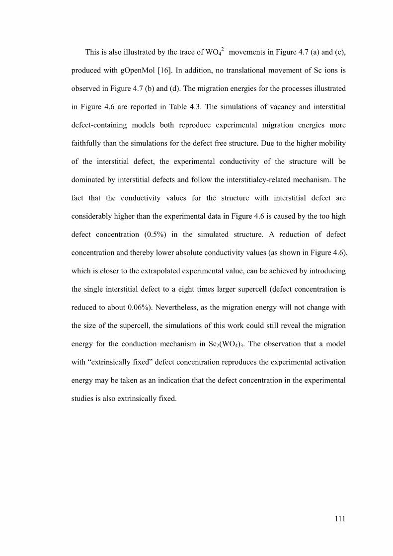
111
This is also illustrated by the trace of WO42− movements in Figure 4.7 (a) and (c),
produced with gOpenMol [16]. In addition, no translational movement of Sc ions is
observed in Figure 4.7 (b) and (d). The migration energies for the processes illustrated
in Figure 4.6 are reported in Table 4.3. The simulations of vacancy and interstitial
defect-containing models both reproduce experimental migration energies more
faithfully than the simulations for the defect free structure. Due to the higher mobility
of the interstitial defect, the experimental conductivity of the structure will be
dominated by interstitial defects and follow the interstitialcy-related mechanism. The
fact that the conductivity values for the structure with interstitial defect are
considerably higher than the experimental data in Figure 4.6 is caused by the too high
defect concentration (0.5%) in the simulated structure. A reduction of defect
concentration and thereby lower absolute conductivity values (as shown in Figure 4.6),
which is closer to the extrapolated experimental value, can be achieved by introducing
the single interstitial defect to a eight times larger supercell (defect concentration is
reduced to about 0.06%). Nevertheless, as the migration energy will not change with
the size of the supercell, the simulations of this work could still reveal the migration
energy for the conduction mechanism in Sc2(WO4)3. The observation that a model
with “extrinsically fixed” defect concentration reproduces the experimental activation
energy may be taken as an indication that the defect concentration in the experimental
studies is also extrinsically fixed.

112
Figure 4.7 Traces of the motion of (a, c) tungstate groups (represented by W atoms) and (b, d) Sc atoms for the NVT simulation of Sc2(WO4)3 structures with (a, b) vacancy defect and (c, d) interstitial defect, based on 15 snapshots over 5 ns period at T=1300K.
Molecular Dynamics simulations of the defect free Sc2(WO4)3 structure as
discussed in chapter 3 [5] yield an activation energy of 1.8 eV, which includes the
generation of one WO42− Frenkel defect and the migration of interstitial defect. In
these simulations only the interstitial ion of a generated Frenkel defect pair was
observed to move before the Frenkel defect vanishes again (by the interstitial ion
meeting a translation copy of the vacancy). Therefore, the estimated formation energy
of WO42− Frenkel defect from Molecular Dynamics simulations is 1.8 – 0.68 = 1.12
eV, similar to the value derived from Mott-Littleton calculations (1.23 eV).

113
4.3.3 Experimental characterization of nonstoichiometric samples
Impedance measurements of nonstoichiometric samples of general brutto formula
Sc2O3 − xWO3, where x = 2.9, 3.0 or 3.1 are shown in Figure 4.8. There is no distinct
difference in conductivity properties between these three samples. It seems that the
intrinsic defect concentration of Sc2(WO4)3 is not notably affected by the minor
deviation from stoichiometric ratio of Sc2O3 : WO3.
The sample with a nominal composition of x = 2.9 contains a small amount of
Sc6WO12: a Rietveld refinement yields a weight fraction of 1.4% Sc6WO12 close to
the value 1.0% to be expected if the excess Sc2O3 is completely converted into
Sc6WO12. Given the low precision of the Rietveld method for this low mass fraction
of the second phase, it may be tentatively concluded that this sample is a composite of
stoichiometric Sc2(WO4)3 and Sc6WO12. For x=3.1 the sample appears to be single
phased according to powder XRD, but as for the x= 2.9 case the observed deviation of
the lattice constants from the stoichiometric case (a minute reduction of b) is hardly
significant. Impedance data accordingly suggest that the conductivity of Sc2(WO4)3
does not change significantly with the variation of Sc2O3:WO3 ratio. Thus the actual
defect concentration may not have been enhanced by these experiments. It cannot be
excluded that the apparent minute conductivity enhancement for “x = 3.1” is
effectively caused by the electronic conductivity of small amounts of unreacted WO3.
Overall, the slight deviations in stoichiometry that may have been achieved (if at all)
are not sufficient to control the defect formation efficiently. The pronounced variation
of literature data on the absolute conductivities (and to some extent also on the
activation energy, see Chapter 3) is probably more efficiently affected by differences
in the compound synthesis and sample preparation.
Furthermore, aliovalent doping experiments (Zr4+, Ti 4+, Ca2+ and Mg2+ in Sc3+

114
site; P5+ in W6+ site) in Sc2(WO4)3 [8] are also found to be unsuccessful. Impurity
phases formed in these systems with negligible effect to the Sc2(WO4)3 lattice
constants, which confirms that these doping strategies have failed to introduce
extrinsic defects in Sc2(WO4)3. Considering the difficulties of nonstoichiometry and
aliovalent doping in Sc2(WO4)3, other doping strategy, e.g. heterointerface doping,
will be studied in the next chapter.
Figure 4.8 Comparison of experimental conductivities of nonstoichiometric samples with formula Sc2O3 − xWO3, where x = 2.9, 3.0 and 3.1. For all samples of this study the activation energies are 0.66eV±0.02eV. The deviating high temperature behaviour for the sample from the previous study [1] might be affected by the differences in the thermal history of the samples and the different nature of the electrodes.
0.7 0.8 0.9 1.0 1.1 1.2 1.3 1.4 1.5 1.6 1.7 1.8 1.9 2.0
-4.0
-3.5
-3.0
-2.5
-2.0
-1.5
-1.0
-0.5
0.0
0.5
Data in Chapter 3x=3.00x=2.90x=3.10
log
(T
/ S
·cm
-1·K
)
103 K / T

115
The sample pellets prepared in this work can only achieve about 70% of the
theoretical density. If higher pressure is used to press the powder into pellet, the pellet
will delaminate from the center. This delamination problem restricted the highest
pressure that could be used for sample preparation and thus it was not possible for us
to further increase the sample density. Our collaborator, Prof. Edwards’ group in US,
solved this problem by using a specially designed equipment to apply a pressure for
the pellet during sintering, through which the sample density could be increased to as
high as 91% of theoretical density. The SEM photographs of three samples with
different densities are shown in Figure 4.9. The sample prepared by this work, as can
be seen from Figure 4.9 (a), has only 70% density and many holes are visible. Figure
4.9 (b) and (c) show two samples prepared without and with external pressure.
Approximately 0.2 MPa pressure is applied to the sample in Figure 4.9 (c) during
sintering at 1100 oC for 24 hours. 91% of theoretical density could be achieved
compared to 74% density without external pressure. The impedance profile of high
density sample shows two semicircles, see Figure 4.10 (a), which correspond to the
bulk conduction and grain boundary conduction respectively; therefore, we can
separate these two effects from the total conductivity. The comparison of
conductivities of this work and Edwards’ work is shown in Figure 4.11. The sample
prepared with lower pressure during preparation (thus lower density) in this work
shows similar conductivity as the grain boundary conduction; whereas, the variation
of the conductivity in the sample prepared at higher pressure follows more the
behaviour of Edwards’ total conductivity curve (and hence grain boundary-dominated
conductivity at low temperatures and a transition to essentially bulk conductivity for
temperatures above 1000 K).

116
(
(

117
Figure 4.9 SEM photographs of Sc2(WO4)3 samples with different density: (a) 70% of theoretical density prepared by this work, (b) and (c) are prepared by Prof. Edwards’ group with density of 74% and 91% respectively.
Figure 4.10 Impedance spectra of two samples at 600 °C: (a) sintered under applied pressure with 91% of theoretical density, (b) sintered with no pressure with 74% of theoretical density.
(
(a)
(b)

118
Figure 4.11 Comparison of this work’s experimental conductivities of stoichiometric samples with Edwards’ work.
4.4 Conclusions
The polyatomic defect formation and migration behavior in Sc2(WO4)3 have been
studied by both computer simulations and electrochemical impedance characterization.
The following conclusions can be reached:
(1) The formation energies of intrinsic defects in Sc2(WO4)3 structure have been
simulated using the GULP code [12]. WO42− Frenkel and Sc2(WO4)3 Schottky defects
are found to have low energies, 1.23 eV and 1.97 eV respectively, which fall into the
range to be possibly self generated as intrinsic defects at elevated temperatures. It has
been shown that the formation of WO42− defect clusters is energetically favorable
compared to individual isolated W and O defects, therefore, the WO42− group as the
conduction species in Sc2(WO4)3 would be possible.
0.7 0.8 0.9 1.0 1.1 1.2 1.3 1.4 1.5 1.6 1.7 1.8 1.9-4.0
-3.5
-3.0
-2.5
-2.0
-1.5
-1.0
-0.5
0.0
0.5
Edwards' workTotalGrainGrain boundary
This workLoad=1tonLoad=5ton
log
(T
/ S
·cm
-1·K
)
103 K / T

119
(2) The migration energies of WO42− vacancy and interstitial defects are studied
by Molecular Dynamics simulations and they both reproduce the experimental data
well; however, due to the higher mobility, the WO42− interstitial defect, which follows
the interstitialcy mechanism, would be the dominant mobile species in
Sc2(WO4)3−type structures.
(3) The impedance characterization experiment shows that nonstoichiometric
doping to Sc2(WO4)3 cannot be achieved effectively. The sample density and thus
conduction behavior will be affected by the pressure used both in sample preparation
and sintering.
References
[1] N. Imanaka, Y. Kobayashi, and G. Y. Adachi, Chem. Lett. 24 (1995) 433.
[2] N. Imanaka et al., Rare Earths '98 315−3 (1999) 331.
[3] N. Imanaka et al., Chem. Mater. 10 (1998) 2006.
[4] J. Köhler, N. Imanaka, and G. Y. Adachi, J. Mater. Chem. 9 (1999) 1357.
[5] Y. K. Zhou et al., Chem. Mater. 20 (2008) 6335.
[6] Y. K. Zhou, R. P. Rao, and S. Adams, Monatsh. Chem. 140 (2009) 1017.
[7] Y. K. Zhou, S. Adams, and A. Neiman, Mater. Res. Soc. Symp. Proc. 1177E (2009) in press.
[8] D. J. Driscoll, M. S. Islam, and P. R. Slater, Solid State Ionics 176 (2005) 539.
[9] A. B. Lidiard, J. Chem. Soc., Faraday Trans. 2 85 (1989) 341.
[10] N. F. Mott, and M. J. Littleton, Trans. Faraday Soc. 34 (1938) 485.
[11] C. Richard, and A. Catlow, JCS Faraday Trans. 2 85 (1989) 335.

120
[12] J. D. Gale, JCS Faraday Trans. 93 (1997) 629.
[13] Materials Studio, version 4.2, Accelrys Inc.: San Diego (2007).
[14] J. P. Perdew, K. Burke, and M. Ernzerhof, Phys. Rev. Lett. 77 (1996) 3865.
[15] A. K. Rappé, and W. A. Goddard, Journal of Physical Chemistry 95 (1991) 3358.
[16] L. Laaksonen, J. Mol. Graph. 10 (1992) 33.

121
Chapter 5
Chapter 5 Polyanion Transport at
Nanostructured Interfaces
5.1 Introduction
Ion conductivity is the primary factor that controls the applicability of ionic
conductors. In Chapter 3 and 4, the polyatomic anion conduction in Sc2(WO4)3 type
structures has been demonstrated with further investigation of defect formation and
migration processes. However, the low value of the conductivity of these materials
restricts their potential applications. As a significant conductivity by the common

122
strategy of homogeneous (aliovalent) doping has not lead to significant conductivity
enhancements [1], the alternative approach of exploiting interface effects is explored
in this section (“heterogeneous doping”). The significant enhancement of ionic
conductivity was observed for various solid electrolyte/insulator and solid electrolyte
1 / solid electrolyte 2 heterojunctions such as LiI−Al2O3 [Liang, Maier] and has also
been demonstrated in artificial CaF2 / BaF2 nanoscale heterostructures [2-5]. There it
has been explained as the consequence of redistribution of mobile ions in the space
charge region, i.e. at the interface of CaF2 / BaF2, F− transferred from BaF2 into CaF2
and created high density of vacancy and interstitial defects on each side respectively
near the surface area. This phenomenon was further comprehensively studied by
defect chemistry modeling [6, 7], bond valence analysis [8] and Molecular Dynamic
simulations [9-12]. These studies indicate that besides the increased concentration of
mobile defects also the change of their mobility plays a relevant role. Another
mechanism to enhance ion conductivity at heterointerface was found in
Yttria-Stabilized Zirconia (YSZ) / SrTiO3 heterostructure[13-15]. Lateral O2− ionic
conductivity was found to be eight orders of magnitude higher at the interfaces than in
the bulk YSZ material. Since there is already high density of extrinsic oxygen
vacancies existing in YSZ, the conductivity cannot be enhanced so much by
heterophase doping. While the original paper attributed the effect to the highly
disordered interface structure [15], a later study [16] suggests that the elastic strain at
the interface due to the mismatch of YSZ and SrTiO3 lattices is responsible for the
enhanced charge carrier mobility.
In this chapter, the WO42−diffusion behaviour at nanoscale Sc2(WO4)3 / CaWO4
heterostructure interfaces will be investigated by Molecular Dynamics simulations.
The choice of the interface orientations in the heterostructure is guided by the

123
calculated attachment and surface energies of Sc2(WO4)3 and CaWO4 structures.
5.2 Methods
Attachment and surface energies were calculated using the Morphology module,
while Molecular Dynamics (MD) simulations were undertaken by the Forcite module,
both in the Materials Studio software suite [17]. Both types of investigations used a
modified UFF universal forcefield [18] as described in section 5.3.1. The
heterostructure was built by attaching selected surfaces of Sc2(WO4)3 and CaWO4.
The scheme for relaxing the heterostructure was shown in Figure 5.3. The
heterostructure was first geometry optimized and then fully relaxed in a NPT
simulation at 600 K for 100 ps. The last frame of the trajectory file was used as the
starting point of a 500 ps NPT simulation production run for the diffusion study.
Integration of the equation of motion has been performed with a Verlet velocity
algorithm [19] in Materials Studio. Time steps have been chosen as 1.0 fs. Coulombic
interactions have been calculated by the Ewald summation method with a cutoff of
12.5 Å and an accuracy of 0.001 kcal/mol and a short range interaction cutoff of 5.61
Å. Temperature was controlled using the Nosé-Hoover thermostat and pressure (for
the case of the NPT simulations) by the Berendsen barostat (Cell mass prefactor =
0.1).

124
5.3 Results and discussion
5.3.1 Forcefield for this simulation
The forcefield used in this chapter is based on the same revised universal
forcefield used in Chapters 3 and 4. Additional Ca – O interaction parameters are
optimized to reproduce the lattice parameters of bulk CaWO4. The optimized
forcefield used the same type of Morse potential function as Equation (3.5) with
parameters: D0(Ca−O)=7 kcal / mol, r0 (Ca−O)= 2.6 Å and y = 12. The calculated
lattice parameters (Table 5.1) and elastic constants (Table 5.2) of CaWO4 are in good
agreement with experimental data.
Table 5.1 Experimental [20] and calculated structural parameters of CaWO4 at room temperature.
Properties Experimental Calculated Relative error (%)
Volume (Å3) 319.1804 310.7077 −2.6545
Lattice a (Å) 5.2425 5.0451 −3.7654
Lattice c (Å) 11.6134 12.2071 5.1122
Table 5.2 Experimental [21] and calculated elastic constants of CaWO4 at room temperature. Elastic constants
(GPa) C11 C12 C13 C16 C33 C44 C66
Experimental 143.87 63.50 56.17 −16.36 130.18 33.61 45.07
Calculated 181.84 97.02 101.32 −32.84 238.18 67.07 58.20

125
5.3.2 Surface energy calculation
As no experimental details on Sc2(WO4)3 / CaWO4 heterointerfaces are
available, planes with low surface energies of these two compounds are studied by
computer simulations to identify suitable attaching interfaces and characterize their
respective attachment energy. Although Sc2(WO4)3 (010) [22] and CaWO4 (101) (112)
(001) [23] are experimentally found to be naturally existing cleavage surfaces, it does
not mean these surfaces have the lowest surface energies. Cleavage surfaces are more
closely related to the attachment energies. The attachment energy (Eatt) [24, 25] is
defined as the energy released when a new slab is attached to the crystal face as
presented in Equation (5.1),
att latt slabE E E (5.1)
where Elatt is the lattice energy, Eslab is the energy of the growth slab.
In contrast, surfaces energies (Esurf) is the energy difference between the slab in
the vacuum and in the crystal as in shown in Equation (5.2),
[ ( ) ( )]
lim2
bulk slabsurf M
E M E ME
S
(5.2)
where M is layer thickness of the slab, Ebulk(M) is the energy of a slab inside the
infinite bulk structure, Eslab is the energy of a slab in vacuum and S is the surface area
of the supercell. There are two surfaces of a slab; therefore S is doubled in the
denominator of Equation (5.2).
Attachment and surface energies of these two compounds are systematically
calculated. The WO4 tetrahedra are always preserved if the surface termination cuts
through them. Selected calculation results are listed in Table 5.3.

126
Table 5.3 Calculated surface energies (γ) of Sc2(WO4)3 and CaWO4. Different terminations of Sc2(WO4)3 (0 1 0) surface (as indicated in Figure 5.1) and CaWO4 (1 0 1) surface (see Figure 5.2) are compared.
Compound Surface Attachment energy (eV) Surface energy (J/m2) Sc2(WO4)3 (0 1 0)a −6.754 0.304
(0 1 0)b −22.691 0.125 (0 1 0)c −22.691 0.125 (1 0 0) −19.205 0.203 (0 0 1) −15.301 0.222 (1 2 1) −15.364 0.226
CaWO4 (1 0 1)a −12.969 0.144 (1 0 1)b −10.799 0.144 (1 0 3) −24.074 0.583 (0 0 1) −11.258 0.848 (2 1 1) −27.159 1.167 (1 1 2) −16.053 1.234 (1 0 2) −54.560 2.371
Figure 5.1 Three terminations of (0 1 0) plane in the Sc2(WO4)3 unit cell, which is shown in the projection along z axis, showing Sc as large, O as small spheres and WO4 tetrahedra.
a
b
c
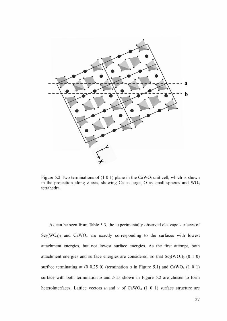
127
Figure 5.2 Two terminations of (1 0 1) plane in the CaWO4 unit cell, which is shown in the projection along z axis, showing Ca as large, O as small spheres and WO4 tetrahedra.
As can be seen from Table 5.3, the experimentally observed cleavage surfaces of
Sc2(WO4)3 and CaWO4 are exactly corresponding to the surfaces with lowest
attachment energies, but not lowest surface energies. As the first attempt, both
attachment energies and surface energies are considered, so that Sc2(WO4)3 (0 1 0)
surface terminating at (0 0.25 0) (termination a in Figure 5.1) and CaWO4 (1 0 1)
surface with both termination a and b as shown in Figure 5.2 are chosen to form
heterointerfaces. Lattice vectors u and v of CaWO4 (1 0 1) surface structure are
a
b

128
defined to be [1 0 −1] and [0 1 0] respectively. The heterointerface is built by
attaching CaWO4 (1 0 1) 6v and 2u to Sc2(WO4)3 a and c using average values for
heterostructure lattices, while the thicknesses of the CaWO4 and Sc2(WO4)3 layers
forming a sandwich structure are chosen to have similar values. The lattice constants
of the 3D periodic 2808 atoms heterolayer supercell are shown in Table 5.4. Then the
heterostructure is relaxed according to the relaxation scheme as shown in Figure 5.3
with fixed cell angles.
There are two different interfaces in this heterostructure. The “upper interface” in
Figure 5.3 uses CaWO4 (1 0 1) termination a so that a layer of WO4 groups are
exposed; in contrast, the “lower interface” adopts CaWO4 (1 0 1) termination b by a
layer of Ca ions. After relaxation, some WO4 groups at the upper interface diffuse
from the Sc2(WO4)3 phase into the top layer of the CaWO4 slab, while no such
tungstate transfer occurs at the lower interface. In order to visualize the extent of
disorder of each element at the heterointerfaces, a plot of the accumulated number of
atoms against the distance from the bottom of the structure (see the structure in Figure
5.4) is used in this work. The accumulated number of atoms at a certain distance is the
total number of that species from the bottom of the structure to that height. If the
atoms in the structure are ordered, the profile will show clean steps; on the contrary,
disordered areas are corresponding to the regions that do not have sharp steps on the
accumulated number of atoms profile. Therefore, as can be seen from Figure 5.4, the
atoms near the upper interface are less ordered than those near the lower interface.
The boundary of Sc2(WO4)3 and CaWO4 at the upper interface becomes blurred.

129
Table 5.4 Heterostructure building strategy.
CaWO4 6v 2u Layer thickness
30.272 Å 26.422 Å 26.353 Å
Sc2(WO4)3 a c Layer thickness
29.049 Å 28.786 Å 26.947 Å
Heterostructure a c b
As built 29.661 Å 27.604 Å 53.300 Å
Geometry optimized 29.320 Å 26.611 Å 52.666 Å
Relaxed at 600K 29.756 Å 26.792 Å 52.693 Å

130
Fig
ure
5.3
Illu
stra
tion
of
the
rela
xati
on s
chem
e fo
r th
e he
tero
stru
ctur
e. T
he i
niti
al s
truc
ture
(le
ft)
is f
irst
geo
met
ry
opti
miz
ed a
nd t
hen
full
y re
laxe
d in
the
NP
T s
imul
atio
ns a
t 60
0K f
or 1
00 p
s. W
ato
ms
are
show
n as
tet
rahe
dra
(Gra
y on
es o
rigi
nall
y be
long
to
CaW
O4,
whi
le d
ark
ones
bel
ong
to S
c 2(W
O4)
3.),
Sc
as g
ray
sphe
res,
Ca
as d
ark
sphe
res
in
the
stru
ctur
e.
Up
per
inte
rfac
e
Low
er in
terf
ace

131
Fig
ure
5.4
Acc
umul
ated
num
ber
of a
tom
s, s
tart
ed f
rom
the
bot
tom
of
the
show
n st
ruct
ure,
of
each
ele
men
t. W
ato
ms
are
show
n as
te
trah
edra
(G
ray
ones
ori
gina
lly
belo
ng to
CaW
O4,
whi
le d
ark
ones
bel
ong
to S
c 2(W
O4)
3.),
Sc
as g
ray
sphe
res,
Ca
as d
ark
sphe
res
in
the
stru
ctur
e
Up
per
inte
rfac
e
Low
er in
terf
ace

132
The diffusion coefficient of WO42− is also affected by the interface. A distance
dependence analysis for the diffusion coefficient of WO42− is shown in Figure 5.5.
The maximum total conductivity of WO42− is not exactly at the interface but about
one layer away from the interface in the Sc2(WO4)3 phase. This is because the
mobility of WO42− is lower in CaWO4 than in Sc2(WO4)3. Although the structure at
the interface is highly disordered, the mobility of WO42− is restricted by interaction
with CaWO4. The WO42− groups of in the Sc2(WO4)3 phase close to the interface are
significantly disordered and (at least for the upper interface) the concentration of
vacancies is enhanced. Both factors contribute to the maximum of the diffusion
coefficient in the Sc2(WO4)3 phase at a distance of about 5 Å from the interface. For
the top layer of the CaWO4 side of the interface the increased disorder may enhance
the diffusion, but the increased concentration of tungstate groups also restricts the
reorientations required for tungstate transport. The anisotropic diffusion coefficients
in x and z directions basically follow the same trend as the total diffusion coefficient;
however, the diffusion coefficient in y direction behave differently at two different
interfaces. As can be seen from Figure 5.5 (c), the “upper interface” allows more
perpendicular diffusions (y direction) than the “lower interface” does.

133
-10 -5 0 5 10 15-11.5
-11.0
-10.5
-10.0
-9.5
-9.0
-8.5
-8.0
-7.5
-7.0(a)
CaWO4
Lo
g (
D /
cm2 ·s
-1)
Sc2(WO
4)3
Distance from the interface / Å
-10 -5 0 5 10 15-11.5
-11.0
-10.5
-10.0
-9.5
-9.0
-8.5
-8.0
-7.5
-7.0(b)
CaWO4
Lo
g (
D /
cm2 ·s
-1)
Sc2(WO
4)3
Distance from the interface / Å
-10 -5 0 5 10 15-11.5
-11.0
-10.5
-10.0
-9.5
-9.0
-8.5
-8.0
-7.5
-7.0(c)
CaWO4
Lo
g (
D /
cm2 ·s
-1)
Sc2(WO
4)3
Distance from the interface / Å

134
Figure 5.5 Variation of the WO4
2− diffusion coefficient against the distance from the interface. (a) is the total diffusion coefficient; while (b), (c) and (d) are anisotropic diffusion coefficients in x, y and z directions respectively. Squares correspond to the “upper interface”, while triangles indicate the “lower interface”. The vertical line indicates the center of the interface, while the horizontal dashed line represents the experimental bulk diffusion coefficient at 600K.
The conductivity of WO42− groups which belong to Sc2(WO4)3 in the
heterostructure after relaxation is estimated by Nernst-Einstein equation (which
implicitly assumes that the tungstate ions move independently; which is a
simplification of the real situation but should bias all displayed values by roughly the
same amount). Compared to experimental conductivity and other structures, the
conductivity is obviously enhanced by heterointerface; in addition, the activation
energy is also drastically reduced to roughly 0.24 eV in comparison with bulk values
for interstitial (0.68 eV) and vacancy (0.74 eV) mechanisms. Despite the pronounced
scatter of these values, this implies that the increased mobility of the tungstate ions in
the less densely packed disordered interface area is a major factor contributing to the
-10 -5 0 5 10 15-11.5
-11.0
-10.5
-10.0
-9.5
-9.0
-8.5
-8.0
-7.5
-7.0(d)
CaWO4
Lo
g (
D /
cm2 ·s
-1)
Sc2(WO
4)3
Distance from the interface / Å

135
enhanced conductivity.
Figure 5.6 Comparison of experimental conductivity and simulated conductivities for Sc2(WO4)3 structure models containing one extra interstitial tungstate, tungstate vacancy, initially no defect and Sc2(WO4)3 at heterointerface.
The traces of the moving WO42− groups in the heterostructure are visualized using
the program gOpenMol [26]. As can be seen from Figure 5.7, the WO42− groups at
about 5 Å from the interface in the Sc2(WO4)3 phase have longer diffusion traces than
those exactly at the interface, which is consistent with the analysis of diffusion
coefficients.
0.5 0.6 0.7 0.8 0.9 1.0 1.1 1.2 1.3 1.4 1.5 1.6 1.7-2.5
-2.0
-1.5
-1.0
-0.5
0.0
0.5
1.0
ExpermentalDefect-freeVacancyinterstitialInterface
log
(T
/ S
·cm
-1·K
)
103 K / T

136
5.4 Conclusions
Figure 5.7 The trace of the motion of W atoms for the NPT simulation of Sc2(WO4)3 at T=600K, based on 20 snapshots over 500 ps simulation time.
Lower interface
CaWO4
Upper interface
Sc2(WO4)3
Sc2(WO4)3

137
Through the Molecular Dynamics studies of the Sc2(WO4)3 / CaWO4 nanoscale
heterostructure, we found that the conductivity of polyatomic WO42− anions can be
enhanced by introducing heterointerfaces. The structure at the interface becomes
disordered by losing the clearly layered arrangement. The maximum conductivity of
WO42− shows up on the Sc2(WO4)3 side at 5 Å from the interface. This maximum
does also occur at interfaces where no redistribution of tungstate groups between the
phases is observed. Thus it may be concluded that in this case the variation of the
charge carrier mobility (due to the combined effects of the disordered structure and
the increased free volume especially on the Sc2(WO4)3 side of the interface) is more
relevant than the variation of the defect concentration.
References
[1] D. J. Driscoll, M. S. Islam, and P. R. Slater, Solid State Ionics 176 (2005) 539.
[2] N. Sata et al., Nature 408 (2000) 946.
[3] N. Y. Jin-Phillipp et al., J. Chem. Phys. 120 (2004) 2375.
[4] X. X. Guo et al., Appl. Phys. Lett. 91 (2007).
[5] X. X. Guo et al., J. Appl. Phys. 105 (2009) 5.
[6] X. X. Guo et al., Phys. Rev. B 76 (2007) 7.
[7] X. X. Guo, and J. Maier, Adv. Funct. Mater. 19 (2009) 96.
[8] S. Adams, and E. S. Tan, Solid State Ionics 179 (2008) 33.
[9] D. C. Sayle et al., Chem. Commun. (2003) 1804.
[10] K. Nomura, and M. Kobayashi, in 9th Euroconference on IonicsIxia, Greece, (2002), pp. 64.

138
[11] K. Nomura, and M. Kobayashi, Ionics 14 (2008) 131.
[12] D. Zahn et al., Journal of Physical Chemistry C 113 (2009) 1315.
[13] X. Guo, Science 324 (2009).
[14] J. Garcia-Barriocanal et al., Science 324 (2009).
[15] J. Garcia-Barriocanal et al., Science 321 (2008) 676.
[16] N. Schichtel et al., Phys. Chem. Chem. Phys. 11 (2009) 3043.
[17] Materials Studio, version 4.2, Accelrys Inc.: San Diego (2007).
[18] A. K. Rappé et al., J. Am. Chem. Soc. 114 (1992) 10024.
[19] L. Verlet, Phys. Rev. 159 (1967) 98.
[20] J. D. Gale, Philos. Mag. B 73 (1996) 3.
[21] M. Gluyas, F. D. Hughes, and B. W. James, J. Phys. D. 6 (1973) 2025.
[22] K. Nassau, H. J. Levinstein, and G. M. Loiacono, J. Phys. Chem. Solids 26 (1965) 1805.
[23] C. Palache, H. Berman, and C. Frondel, Dana's System of Minearology Vol. 2, 7th edn. Ney York: Wiley, 1951, pp. 1073.
[24] DOCHERTY R et al., J. Phys. D. Appl. Phys. 24 (1991) 89.
[25] Z. Berkovitch-Yellin, J. Am. Chem. Soc. 107 (1985) 8239.
[26] L. Laaksonen, J. Mol. Graph. 10 (1992) 33.

139
Chapter 6
Chapter 6 Conclusion and Future
Work
6.1 Conclusion
The overall objective of this research was to explore the conduction mechanism
in Sc2(WO4)3 and related oxides. A clue to the local mobility of the WO42− group
turned out to be the rare negative thermal expansion (NTE). In this work, it is
confirmed that the overall thermal expansion remained negative throughout the
temperature range of our investigations up to 1300K. Since the W−O bond is more

140
covalent than Sc−O, it is to be expected that WO4 will be a more rigid unit than ScO6.
In line with this expectation our Rietveld refinements yielded an apparent reduction of
W−O bond lengths (as a sign of correlated large amplitude rocking motion), but not of
the Sc−O bond length at elevated temperatures. The validity of the modified universal
forcefield used in this work can be verified by reproducing NTE when T ≤ 500K and
reproducing the orthorhombic to monoclinic phase transition in Sc2(WO4)3 under
compression. Although the phase transition pressure is found 0.55 GPa higher than the
experimental one, the lattice compressibility in the simulation of both phases are
consistent with the experimental trend.
From a synopsis of these results we tentatively concluded that WO42− is the rigid
unit with the lowest charge in the system and its pronounced rocking motion might be
a sign of a potential WO42− mobility. Through the combination of X-ray data,
impedance spectroscopy, Tubandt-type DC electrolysis, molecular dynamics
simulations and their bond valence analysis we could then establish a model for the
peculiar charge transport mechanism in Sc2(WO4)3−type solid electrolytes:
• Tubandt-type measurements demonstrated that the effective charge carrier is
an anion.
• Molecular dynamics simulations and a bond valence pathway analysis
accordingly found pathways for the motion of tungstate groups, but not for Sc3+.
• The elementary transport steps combined features of an intersticialcy
mechanism with a “rock and roll” component.
• The proposed “rock and roll” WO42− ion transport mechanism is also
consistent with the experimental results in this work and in the literature.
Our molecular dynamics (MD) simulations that started from a defect-free
Sc2(WO4)3 structure require a rare high energy defect creation process, and thereby

141
lead to an activation energy of the MD simulated ionic conductivity that is
considerably higher than the experimental value. The formation energies of intrinsic
defects in Sc2(WO4)3 structure were simulated by the Mott-Littleton approach. WO42−
Frenkel and Sc2(WO4)3 Schottky defects were found to have low energies, 1.23 eV
and 1.97 eV respectively, which fell into the range to be possibly self generated as
intrinsic defects at elevated temperatures. It was shown that the formation of WO42−
defect clusters was energetically favorable compared to individual isolated W and O
defects; therefore, the WO42− group as the conduction species in Sc2(WO4)3 would be
possible. In order to find out the migration energy of the defects, we performed MD
simulations on scandium tungstate structures in structure models with built-in
tungstate vacancies and interstitial defects. Compared to our previous simulations on
defect-free Sc2(WO4)3 structure (EA = 1.80 eV), the diffusion activation energy
obtained from artificially induced defect structures (0.68 eV for interstitial and 0.74
eV for vacancy) is lower and closer to the experimental values (0.67 eV), which
suggests that the experimentally observed activation energy represents the migration
energy of tungstate defects, while the formation of intrinsic defects is found only for T
≥ 1300 K. Due to the higher mobility, the WO42− interstitial defect, which follows the
interstitialcy mechanism, would be the dominant mobile species in Sc2(WO4)3-type
structures.
Thus, we found that Sc2(WO4)3 is indeed a prototype of a new class of ion
conducting solids, but that the mobile charge carriers are tungstate polyatomic anions,
not trivalent cations. The proposed mechanism might be regarded as an O2− vehicle
mechanism, but it does not involve oxide ion vacancies or interstitials; therefore, no
dependence of the O2 partial pressure is to be expected in polarization experiments.
Further investigation of the WO42− diffusion behavior at Sc2(WO4)3/CaWO4

142
heterostructure interfaces were undertaken by Molecular Dynamics simulations.
Structures of both materials became disordered near the interface. WO42− conductivity
was significantly enhanced near the interface; however the maximum conductivity did
not show up exactly at the interface but located at about 5 Å away from the interface
on the Sc2(WO4)3 side.
6.2 Future directions
It should be pointed out that mainly Sc2(WO4)3 as the prototype of the structure
family was studied in this work. The conduction mechanism of further isostructural or
structurally related oxides is also expected to be investigated in the future. It may be
expected that more examples of a polyatomic anion transport mechanism have been
overlooked so far. A limitation for the application of Sc2(WO4)3 type oxides is that
their conductivity is relatively low compared to other technically used solid
electrolytes. To enhance the conductivity, several methods are proposed as follows for
future studies:
• Use nonstoichiometric and aliovalent doping to induce more WO42− defects
in the structure. Although it has been shown that aliovalent doping such as Ca2+ and
Zr4+ in Sc3+ site of Sc2(WO4)3 is energetically unfavorable [1], more ions and
synthetic methods are expected to be studied.
• Exploit interface effects with other WO42− conductors, because WO4
2− groups
will diffuse across the interface and introduce more defects on both sides as
demonstrated in this work.
• Produce nano-particles by ball milling to introduce more grain boundaries in
the material to exploit the enhanced defect concentration in the vicinity of surfaces

143
and interfaces of nanostructured materials.
The application of related “trivalent cation” conductors has been proposed by
Imanaka and coworkers in CO2 gas sensors; however the “trivalent cation” conductor
in this application is not Sc2(WO4)3 type oxides but (Al0.2Zr0.8)20/19Nb(PO4)3 [2] which
adopts the NASICON structure. The setup of this sensor is sketched in Figure 6.1. It
was claimed that the Al3+ conduction plays a role in this cell; however, this is
questionable because NASICON is also a good Li+ conductor. If Al3+ cannot – as
postulated – act as the charge carrier in (Al0.2Zr0.8)20/19Nb(PO4)3, this sensor will still
work but should be explained as based on Li+ and an O2– conductor.
Figure 6.1 Cross−sectional view of the CO2 sensor cell. Reproduced from Ref [2].

144
The development of devices utilizing the polyanion conductivity of the scandium
tungstate type oxides is not experimentally studied in this thesis; however, two
possible applications of WO42− solid conductors as WO4
2− concentration sensor and
WO3 sensor are proposed here (cf. Figure 6.2 and Figure 6.3). The difference of
WO42− concentrations between a reference electrode and a measuring electrode
according to Equation (6.1) will cause a voltage
2
42
4
( )ln[ ]
'( )
c WORTU
nF c WO
, (6.1)
where R is the gas constant, T is temperature, n is the charge number of the charge
carrier (here n=2 for WO42−), F is the Faraday constant, c(WO4
2−) is the concentration
of WO42− to be measured. c’(WO4
2−) is the reference concentration of WO42−. The cell
voltage would change with the concentration of WO42− at the measuring side. The cell
in Figure 6.2 can be used to measure WO42− ion concentration in high temperature
liquids, solutions or melts using low melting point tungstate melt, e.g. Na2WO4
(melting point 698°C), as reference; while Figure 6.3 is a sensor for WO3 vapor
partial pressure in air or other oxygen containing gas mixtures with known oxygen
partial pressure. Porous platinum layer serves as a catalyst for the reaction as shown
in Equation (6.2)
23 2 4
12
2
PtWO O e WO . (6.2)
The concentration of WO42− on the Pt electrode will depend on the partial
pressure of WO3 vapor.

145
References
[1] D. J. Driscoll, M. S. Islam, and P. R. Slater, Solid State Ionics 176 (2005) 539.
[2] S. Tamura et al., Sens. Actuators B Chem. 108 (2005) 359.
Figure 6.2 Design of a WO42− concentration sensor based on WO4
2− solid electrolytes.
Figure 6.3 Design of a WO3 gas sensor based on WO42− solid electrolytes.
Cell Voltage
Pt electrode Low temperature melt with fixed WO4
2− ion concentra- tion as reference
Sc2(WO4)3
Melt with unknown tungstate concentration
Cell Voltage Sc2(WO4)3
Gas to be analyzed Porous Pt layer serving both as electrode and catalyst
Reference electrode

146
Appendix
Table A.1 Atomic fraction coordinates of Sc2(WO4)3 at 11 to 1300K.
Name X Y Z Uiso 11K
Sc1 0.46751(34) 0.37951(25) 0.2504(4) 0.0099(11) W1 0.250000 0.000000 0.47376(14) 0.00915(26) W2 0.11800(10) 0.35550(8) 0.39566(11) 0.00915(26) O1 0.0997(11) 0.1406(9) 0.0783(11) 0.0154(16) O2 0.1303(13) 0.0620(7) 0.3630(11) 0.0154(16) O3 0.0070(12) 0.2633(9) 0.3166(10) 0.0154(16) O4 0.3350(11) 0.4032(7) 0.0770(11) 0.0154(16) O5 0.0693(10) 0.4734(8) 0.3204(11) 0.0154(16) O6 0.2983(12) 0.3318(8) 0.3583(11) 0.0154(16)
50K
Sc1 0.46743(34) 0.37940(24) 0.2501(4) 0.0076(11) W1 0.250000 0.000000 0.47377(14) 0.00828(25) W2 0.11788(10) 0.35549(8) 0.39576(11) 0.00828(25) O1 0.0979(11) 0.1411(8) 0.0801(11) 0.0146(16) O2 0.1302(13) 0.0624(7) 0.3651(11) 0.0146(16) O3 0.0070(11) 0.2636(9) 0.3173(10) 0.0146(16) O4 0.3351(11) 0.4021(7) 0.0779(11) 0.0146(16) O5 0.0685(10) 0.4737(8) 0.3212(11) 0.0146(16) O6 0.2985(11) 0.3331(8) 0.3585(10) 0.0146(16)

147
100K
Sc1 0.46711(35) 0.37979(25) 0.2499(4) 0.0067(11) W1 0.250000 0.000000 0.47381(15) 0.00802(26) W2 0.11794(10) 0.35566(8) 0.39529(11) 0.00802(26) O1 0.1014(12) 0.1384(9) 0.0803(12) 0.0173(16) O2 0.1257(14) 0.0620(8) 0.3637(12) 0.0173(16) O3 0.0023(12) 0.2630(9) 0.3167(11) 0.0173(16) O4 0.3356(11) 0.3997(8) 0.0756(11) 0.0173(16) O5 0.0667(10) 0.4765(9) 0.3193(12) 0.0173(16) O6 0.2988(12) 0.3328(8) 0.3553(11) 0.0173(16)
150K
Sc1 0.46777(22) 0.37931(16) 0.24986(27) 0.0081(7) W1 0.250000 0.000000 0.47351(9) 0.00850(17) W2 0.11794(6) 0.35551(5) 0.39536(7) 0.00850(17) O1 0.1006(7) 0.1401(6) 0.0791(7) 0.0175(10) O2 0.1321(8) 0.0627(5) 0.3624(7) 0.0175(10) O3 0.0035(7) 0.2623(6) 0.3161(7) 0.0175(10) O4 0.3351(7) 0.3998(5) 0.0760(7) 0.0175(10) O5 0.0670(6) 0.4736(5) 0.3207(7) 0.0175(10) O6 0.2976(7) 0.3320(5) 0.3551(7) 0.0175(10)
200K
Sc1 0.46871(25) 0.37973(18) 0.24990(31) 0.00874 W1 0.250000 0.000000 0.47366(10) 0.00822 W2 0.11774(7) 0.35565(6) 0.39513(8) 0.00822 O1 0.1064(9) 0.1399(6) 0.0826(9) 0.0275(14) O2 0.1344(10) 0.0643(6) 0.3614(9) 0.0275(14) O3 0.0014(9) 0.2621(7) 0.3144(8) 0.0275(14) O4 0.3387(8) 0.3968(5) 0.0734(8) 0.0275(14) O5 0.0643(7) 0.4744(6) 0.3184(9) 0.0275(14) O6 0.3015(8) 0.3305(6) 0.3534(8) 0.02096
250K
Sc1 0.46876(22) 0.37982(16) 0.25000(27) 0.0086(7) W1 0.250000 0.000000 0.47325(9) 0.01046(17) W2 0.11714(7) 0.35552(5) 0.39481(7) 0.01046(17) O1 0.0996(7) 0.1408(6) 0.0804(8) 0.0236(11) O2 0.1358(8) 0.0661(5) 0.3633(8) 0.0236(11) O3 0.0051(8) 0.2623(6) 0.3166(7) 0.0236(11) O4 0.3356(7) 0.4014(5) 0.0737(7) 0.0236(11) O5 0.0652(7) 0.4744(6) 0.3205(7) 0.0236(11)

148
O6 0.3001(8) 0.3308(5) 0.3560(7) 0.0236(11)
300K Sc1 0.46741(31) 0.38092(21) 0.2489(4) 0.0149(10) W1 0.250000 0.000000 0.47322(13) 0.01428(23) W2 0.11649(9) 0.35592(7) 0.39449(10) 0.01428(23) O1 0.0908(9) 0.1366(7) 0.0768(10) 0.0216(14) O2 0.1352(11) 0.0655(6) 0.3660(10) 0.0216(14) O3 0.0098(10) 0.2640(8) 0.3186(9) 0.0216(14) O4 0.3332(10) 0.4058(6) 0.0804(10) 0.0216(14) O5 0.0684(9) 0.4750(7) 0.3251(10) 0.0216(14) O6 0.2970(10) 0.3395(7) 0.3544(9) 0.0216(14)
350K
Sc1 0.46750(32) 0.38094(22) 0.2484(4) 0.0169(10) W1 0.250000 0.000000 0.47288(13) 0.01551(24) W2 0.11609(9) 0.35601(7) 0.39406(10) 0.01551(24) O1 0.0903(10) 0.1358(7) 0.0760(10) 0.0258(14) O2 0.1365(11) 0.0673(7) 0.3680(11) 0.0258(14) O3 0.0091(11) 0.2633(8) 0.3195(10) 0.0258(14) O4 0.3326(10) 0.4070(7) 0.0782(10) 0.0258(14) O5 0.0682(9) 0.4751(7) 0.3240(10) 0.0258(14) O6 0.2975(11) 0.3401(7) 0.3536(10) 0.0258(14)
400K
Sc1 0.46764(32) 0.38098(22) 0.2488(4) 0.0185(10) W1 0.250000 0.000000 0.47255(13) 0.01708(24) W2 0.11562(9) 0.35615(7) 0.39366(10) 0.01708(24) O1 0.0906(10) 0.1350(7) 0.0751(10) 0.0290(14) O2 0.1379(11) 0.0677(7) 0.3676(11) 0.0290(14) O3 0.0076(11) 0.2641(8) 0.3189(10) 0.0290(14) O4 0.3336(10) 0.4069(7) 0.0789(10) 0.0290(14) O5 0.0662(9) 0.4764(8) 0.3243(10) 0.0290(14) O6 0.2940(11) 0.3404(7) 0.3523(10) 0.0290(14)
450K
Sc1 0.46788(33) 0.38135(22) 0.2485(4) 0.0187(11) W1 0.250000 0.000000 0.47234(14) 0.01873(25) W2 0.11519(10) 0.35624(7) 0.39323(10) 0.01873(25) O1 0.0922(10) 0.1343(8) 0.0743(11) 0.0318(15) O2 0.1403(11) 0.0693(7) 0.3676(11) 0.0318(15) O3 0.0090(11) 0.2634(8) 0.3198(10) 0.0318(15) O4 0.3327(10) 0.4058(7) 0.0778(10) 0.0318(15)
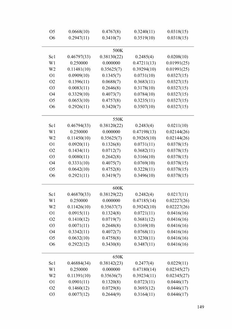
149
O5 0.0668(10) 0.4767(8) 0.3240(11) 0.0318(15) O6 0.2947(11) 0.3410(7) 0.3519(10) 0.0318(15)
500K
Sc1 0.46797(33) 0.38130(22) 0.2485(4) 0.0208(10) W1 0.250000 0.000000 0.47211(13) 0.01991(25) W2 0.11481(10) 0.35625(7) 0.39294(10) 0.01991(25) O1 0.0909(10) 0.1345(7) 0.0731(10) 0.0327(15) O2 0.1396(11) 0.0688(7) 0.3683(11) 0.0327(15) O3 0.0083(11) 0.2646(8) 0.3178(10) 0.0327(15) O4 0.3329(10) 0.4073(7) 0.0784(10) 0.0327(15) O5 0.0653(10) 0.4757(8) 0.3235(11) 0.0327(15) O6 0.2926(11) 0.3420(7) 0.3507(10) 0.0327(15)
550K
Sc1 0.46794(33) 0.38120(22) 0.2483(4) 0.0211(10) W1 0.250000 0.000000 0.47198(13) 0.02144(26) W2 0.11450(10) 0.35625(7) 0.39265(10) 0.02144(26) O1 0.0920(11) 0.1326(8) 0.0731(11) 0.0378(15) O2 0.1434(11) 0.0712(7) 0.3682(11) 0.0378(15) O3 0.0080(11) 0.2642(8) 0.3166(10) 0.0378(15) O4 0.3331(10) 0.4075(7) 0.0769(10) 0.0378(15) O5 0.0642(10) 0.4752(8) 0.3228(11) 0.0378(15) O6 0.2921(11) 0.3419(7) 0.3496(10) 0.0378(15)
600K
Sc1 0.46870(33) 0.38129(22) 0.2482(4) 0.0217(11) W1 0.250000 0.000000 0.47185(14) 0.02227(26) W2 0.11426(10) 0.35637(7) 0.39242(10) 0.02227(26) O1 0.0915(11) 0.1324(8) 0.0721(11) 0.0416(16) O2 0.1410(12) 0.0719(7) 0.3681(12) 0.0416(16) O3 0.0071(11) 0.2648(8) 0.3169(10) 0.0416(16) O4 0.3342(11) 0.4072(7) 0.0768(11) 0.0416(16) O5 0.0632(10) 0.4758(8) 0.3230(11) 0.0416(16) O6 0.2922(12) 0.3430(8) 0.3487(11) 0.0416(16)
650K
Sc1 0.46884(34) 0.38142(23) 0.2477(4) 0.0229(11) W1 0.250000 0.000000 0.47180(14) 0.02345(27) W2 0.11391(10) 0.35636(7) 0.39234(11) 0.02345(27) O1 0.0901(11) 0.1320(8) 0.0723(11) 0.0446(17) O2 0.1460(12) 0.0729(8) 0.3693(12) 0.0446(17) O3 0.0077(12) 0.2644(9) 0.3164(11) 0.0446(17)

150
O4 0.3341(11) 0.4065(7) 0.0767(11) 0.0446(17) O5 0.0632(11) 0.4759(8) 0.3239(12) 0.0446(17) O6 0.2918(12) 0.3439(8) 0.3477(11) 0.0446(17)
700K
Sc1 0.46887(34) 0.38131(23) 0.2477(4) 0.0231(11) W1 0.250000 0.000000 0.47180(14) 0.02496(28) W2 0.11358(10) 0.35647(7) 0.39203(11) 0.02496(28) O1 0.0905(11) 0.1314(8) 0.0714(12) 0.0491(17) O2 0.1476(12) 0.0730(8) 0.3703(12) 0.0491(17) O3 0.0055(12) 0.2640(9) 0.3175(11) 0.0491(17) O4 0.3345(11) 0.4065(8) 0.0761(11) 0.0491(17) O5 0.0618(11) 0.4766(9) 0.3239(12) 0.0491(17) O6 0.2911(12) 0.3451(8) 0.3480(11) 0.0491(17)
750K
Sc1 0.4698(4) 0.38118(24) 0.2478(4) 0.0249(11) W1 0.250000 0.000000 0.47167(14) 0.02599(29) W2 0.11342(11) 0.35649(7) 0.39182(11) 0.02599(29) O1 0.0904(12) 0.1300(8) 0.0703(12) 0.0530(17) O2 0.1481(12) 0.0733(8) 0.3697(13) 0.0530(17) O3 0.0066(12) 0.2646(9) 0.3164(11) 0.0530(17) O4 0.3356(12) 0.4061(8) 0.0763(12) 0.0530(17) O5 0.0618(11) 0.4759(9) 0.3240(12) 0.0530(17) O6 0.2928(13) 0.3462(8) 0.3459(12) 0.0530(17)
800K
Sc1 0.4700(4) 0.38130(24) 0.2478(4) 0.0256(12) W1 0.250000 0.000000 0.47159(15) 0.02612(33) W2 0.11317(11) 0.35639(8) 0.39151(11) 0.02612(33) O1 0.0905(12) 0.1288(9) 0.0689(12) 0.0551(18) O2 0.1501(12) 0.0746(8) 0.3718(13) 0.0551(18) O3 0.0058(12) 0.2637(9) 0.3152(12) 0.0551(18) O4 0.3361(12) 0.4067(8) 0.0758(12) 0.0551(18) O5 0.0603(11) 0.4752(9) 0.3224(13) 0.0551(18) O6 0.2918(13) 0.3461(9) 0.3435(12) 0.0551(18)
850K
Sc1 0.4696(4) 0.38149(25) 0.2474(5) 0.0252(12) W1 0.250000 0.000000 0.47144(15) 0.02750(31) W2 0.11304(11) 0.35645(8) 0.39126(11) 0.02750(31) O1 0.0911(13) 0.1280(9) 0.0681(13) 0.0599(19) O2 0.1515(13) 0.0749(8) 0.3720(14) 0.0599(19)

151
O3 0.0068(13) 0.2648(10) 0.3148(12) 0.0599(19) O4 0.3345(12) 0.4054(8) 0.0756(12) 0.0599(19) O5 0.0582(12) 0.4762(9) 0.3227(13) 0.0599(19) O6 0.2911(13) 0.3473(9) 0.3433(13) 0.0599(19)
900K
Sc1 0.4703(4) 0.38180(25) 0.2469(5) 0.0262(12) W1 0.250000 0.000000 0.47133(15) 0.02815(31) W2 0.11298(11) 0.35645(8) 0.39118(12) 0.02815(31) O1 0.0918(13) 0.1270(9) 0.0682(13) 0.0622(19) O2 0.1520(13) 0.0756(9) 0.3722(14) 0.0622(19) O3 0.0047(13) 0.2646(10) 0.3155(12) 0.0622(19) O4 0.3351(13) 0.4052(8) 0.0732(13) 0.0622(19) O5 0.0592(12) 0.4749(10) 0.3215(13) 0.0622(19) O6 0.2919(14) 0.3479(9) 0.3419(13) 0.0622(19)
950K
Sc1 0.4707(4) 0.38197(25) 0.2468(5) 0.0275(12) W1 0.250000 0.000000 0.47137(16) 0.02924(32) W2 0.11289(12) 0.35635(8) 0.39097(12) 0.02924(32) O1 0.0907(13) 0.1263(9) 0.0666(13) 0.0658(20) O2 0.1539(13) 0.0745(9) 0.3722(14) 0.0658(20) O3 0.0050(13) 0.2656(10) 0.3140(12) 0.0658(20) O4 0.3345(13) 0.4058(9) 0.0737(13) 0.0658(20) O5 0.0569(12) 0.4735(10) 0.3211(13) 0.0658(20) O6 0.2921(14) 0.3474(9) 0.3398(13) 0.0658(20)
1000K
Sc1 0.4704(4) 0.38190(26) 0.2472(5) 0.0267(12) W1 0.250000 0.000000 0.47122(16) 0.02996(33) W2 0.11275(12) 0.35638(8) 0.39088(12) 0.02996(33) O1 0.0913(13) 0.1269(9) 0.0659(14) 0.0681(20) O2 0.1535(13) 0.0749(9) 0.3736(15) 0.0681(20) O3 0.0030(13) 0.2649(10) 0.3139(13) 0.0681(20) O4 0.3353(13) 0.4050(9) 0.0756(13) 0.0681(20) O5 0.0548(12) 0.4738(10) 0.3205(14) 0.0681(20) O6 0.2897(14) 0.3478(10) 0.3398(14) 0.0681(20)
1050K
Sc1 0.4708(4) 0.38198(26) 0.2477(5) 0.0290(12) W1 0.250000 0.000000 0.47111(16) 0.03109(34) W2 0.11256(12) 0.35641(8) 0.39095(12) 0.03109(34) O1 0.0929(14) 0.1264(10) 0.0668(14) 0.0721(21)

152
O2 0.1523(14) 0.0753(9) 0.3718(15) 0.0721(21) O3 0.0053(13) 0.2655(10) 0.3138(13) 0.0721(21) O4 0.3353(14) 0.4061(9) 0.0759(14) 0.0721(21) O5 0.0515(13) 0.4729(10) 0.3190(14) 0.0721(21) O6 0.2888(15) 0.3484(10) 0.3385(14) 0.0721(21)
1100K
Sc1 0.4708(4) 0.38216(26) 0.2472(5) 0.0285(13) W1 0.250000 0.000000 0.47102(17) 0.03266(35) W2 0.11250(12) 0.35645(9) 0.39070(12) 0.03266(35) O1 0.0935(14) 0.1276(10) 0.0672(14) 0.0751(22) O2 0.1551(14) 0.0781(9) 0.3743(15) 0.0751(22) O3 0.0051(14) 0.2646(11) 0.3129(13) 0.0751(22) O4 0.3340(14) 0.4069(9) 0.0740(14) 0.0751(22) O5 0.0518(13) 0.4723(10) 0.3181(14) 0.0751(22) O6 0.2899(15) 0.3487(10) 0.3402(14) 0.0751(22)
1150K
Sc1 0.4712(4) 0.38253(26) 0.2469(5) 0.0284(12) W1 0.250000 0.000000 0.47091(17) 0.0335(4) W2 0.11236(12) 0.35634(9) 0.39043(12) 0.0335(4) O1 0.0937(14) 0.1277(10) 0.0671(14) 0.0776(22) O2 0.1529(14) 0.0779(9) 0.3756(15) 0.0776(22) O3 0.0034(14) 0.2635(11) 0.3131(13) 0.0776(22) O4 0.3351(14) 0.4063(9) 0.0740(14) 0.0776(22) O5 0.0512(13) 0.4734(10) 0.3212(14) 0.0776(22) O6 0.2921(15) 0.3481(10) 0.3393(14) 0.0776(22)
1200K
Sc1 0.4709(4) 0.38211(27) 0.2462(5) 0.0284(13) W1 0.250000 0.000000 0.47095(17) 0.0344(4) W2 0.11232(13) 0.35633(9) 0.39033(13) 0.0344(4) O1 0.0943(14) 0.1283(10) 0.0664(15) 0.0797(22) O2 0.1536(14) 0.0768(9) 0.3720(16) 0.0797(22) O3 0.0026(14) 0.2641(11) 0.3141(14) 0.0797(22) O4 0.3377(14) 0.4050(9) 0.0737(14) 0.0797(22) O5 0.0520(13) 0.4731(11) 0.3215(14) 0.0797(22) O6 0.2928(15) 0.3479(10) 0.3417(15) 0.0797(22)
1250K
Sc1 0.4712(4) 0.38197(27) 0.2463(5) 0.0288(13) W1 0.250000 0.000000 0.47120(18) 0.0349(4) W2 0.11206(13) 0.35626(9) 0.38998(13) 0.0349(4)

153
O1 0.0960(15) 0.1287(10) 0.0682(15) 0.0770(23) O2 0.1541(14) 0.0757(10) 0.3724(16) 0.0770(23) O3 0.0038(14) 0.2652(11) 0.3156(14) 0.0770(23) O4 0.3365(14) 0.4049(9) 0.0729(14) 0.0770(23) O5 0.0541(14) 0.4732(11) 0.3220(15) 0.0770(23) O6 0.2889(16) 0.3473(11) 0.3414(15) 0.0770(23)
1300K
Sc1 0.4722(5) 0.38263(29) 0.2475(6) 0.0272(14) W1 0.250000 0.000000 0.47083(19) 0.0345(4) W2 0.11202(14) 0.35630(10) 0.39020(14) 0.0345(4) O1 0.0981(16) 0.1274(11) 0.0673(16) 0.0831(24) O2 0.1540(15) 0.0776(10) 0.3750(18) 0.0831(24) O3 0.0035(15) 0.2666(12) 0.3100(15) 0.0831(24) O4 0.3367(16) 0.4050(10) 0.0733(16) 0.0831(24) O5 0.0511(14) 0.4717(11) 0.3159(16) 0.0831(24) O6 0.2944(17) 0.3456(11) 0.3424(16) 0.0831(24)

154
Figure A.1 Refinement of Sc2(WO4)3 structure at (a) 800K with final Rwp=6.03% and (b) 1300K with final Rwp=6.06%. Observed (×), calculated (line), and Observed − calculated (lower line). The insets show the details of the refinement result in the 2 theta range from 18° to 31°.
(a)
(b)
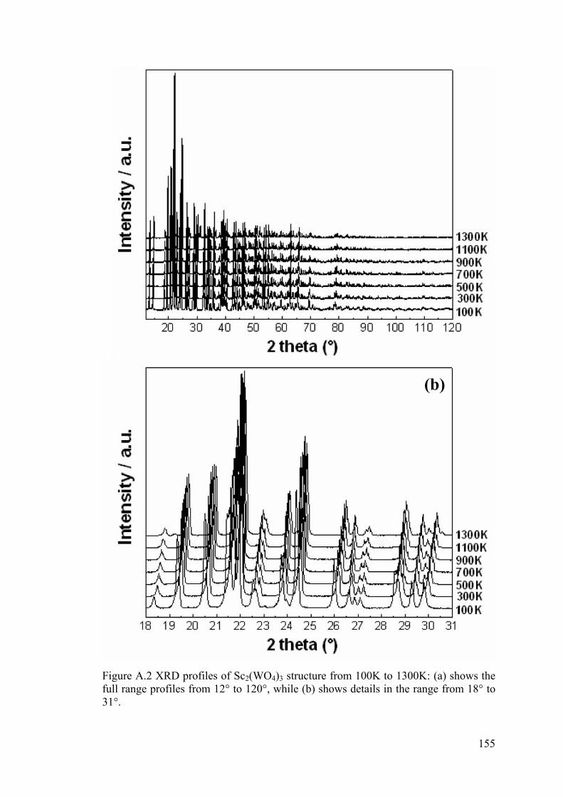
155
Figure A.2 XRD profiles of Sc2(WO4)3 structure from 100K to 1300K: (a) shows the full range profiles from 12° to 120°, while (b) shows details in the range from 18° to 31°.
(b)
(a)


