Download - Phosphorus index project overview collick
Phosphorus Index Project Overview: Refining and Harmonizing Phosphorus Indices in the Chesapeake Bay Region to Improve Critical Source
Area Identification and to Address Nutrient Management Priorities
Presented by Amy S. CollickAgriculture, Food, and Resource SciencesUniversity of Maryland Eastern Shore (UMES)
CollaboratorsUniversity of Maryland Eastern Shore
A. Allen, A. CollickPasture Systems and Watershed Management Research Unit, USDA‐ARS
P. Kleinman, T. Veith, R. Bryant, T. Buda, J. Liu, M. AminPennsylvania State University
D. Beegle, J. WeldVirginia Tech
Z. Easton, D. Fuka, M. ReiterCornell University
Q. Ketterings, K. Czymmek, S. Cela, S. CrittendenUniversity of Delaware
A. Shober, K. Clark, S. TingleWest Virginia University
T. BasdenUniversity of Kentucky
J. McGrath
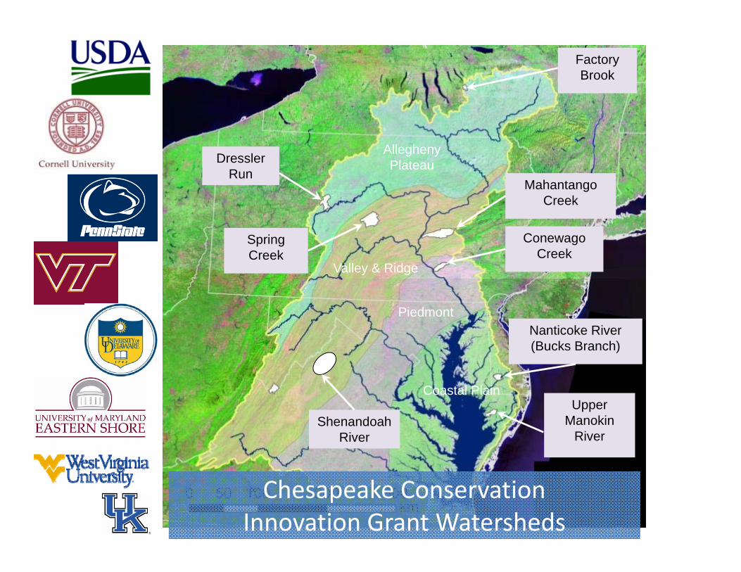
Spring Creek
MahantangoCreek
ConewagoCreek
Allegheny PlateauDressler
Run
Nanticoke River(Bucks Branch)
Upper Manokin
River
Factory Brook
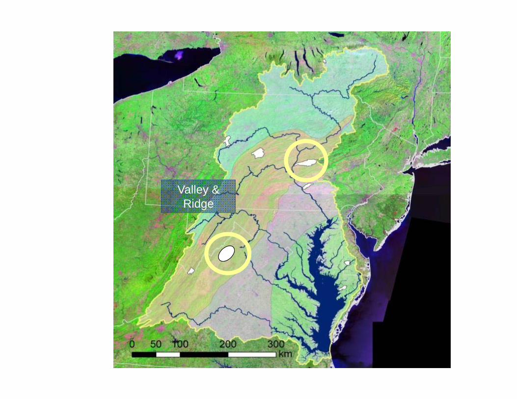
Valley & Ridge
Piedmont
Coastal Plain
Shenandoah River
Chesapeake Conservation Innovation Grant Watersheds
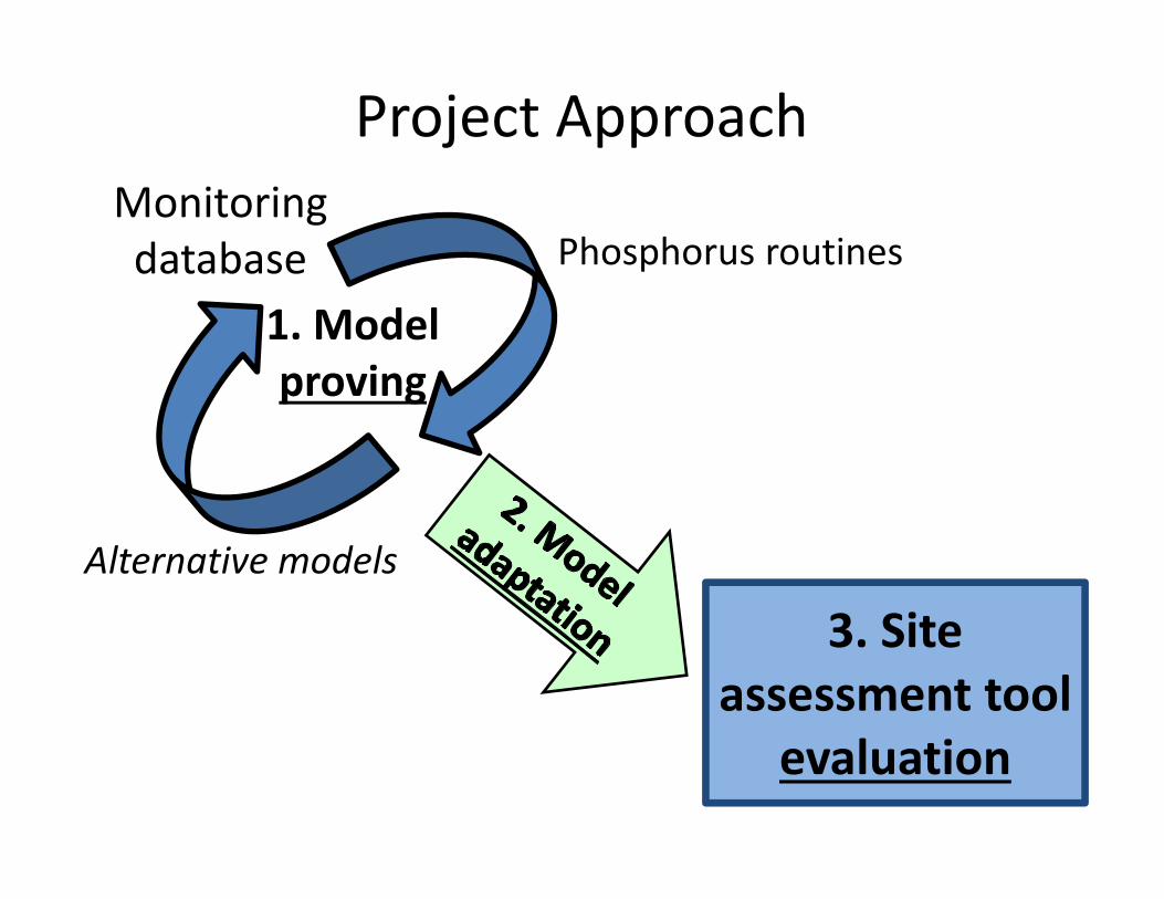
1. Model proving
Monitoring database
3. Site assessment tool
evaluation
Project Approach
Phosphorus routines
Alternative models

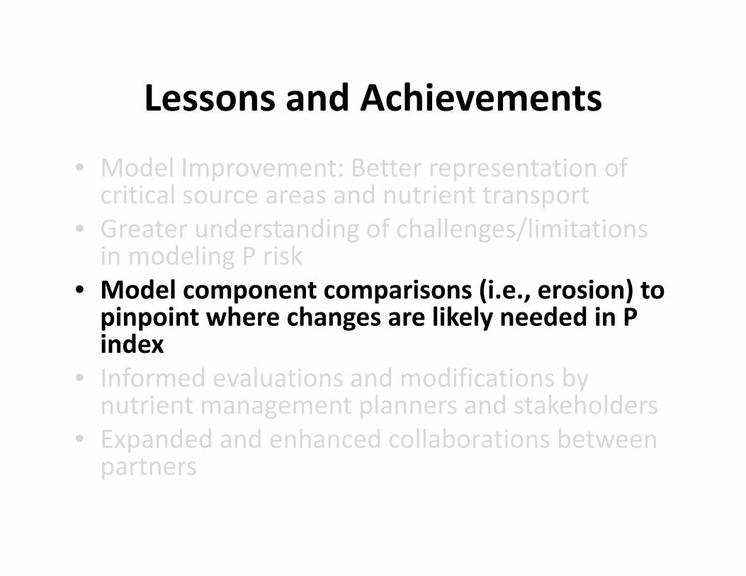
Lessons and Achievements
• Model Improvement: Better representation of critical source areas and nutrient transport
• Greater understanding of challenges/limitations in modeling P risk
• Model component comparisons (i.e., erosion) to pinpoint where changes are likely needed in P index
• Informed evaluations and modifications by nutrient management planners and stakeholders
• Expanded and enhanced collaborations between partners
Valley & Ridge

This is what we must represent
177
144 44
1
<1
Soil P – mg kg-1
Runoff – litersP loss – kg P ha-1 yr-1
92
Buda et al. JEQ, 2009
Lowest field is now a CREP buffer that
continues to yield largest P loads
4620
DPDPDP
8
DPDPDP78

Hydrologic Routine Testing – Mahantango Creek
• Similar outlet discharge hydrographs
• Better spatial distribution of runoff with TopoSWAT
• Improved identification of nutrient sources with TopoSWAT
Standard SWAT
WE38 outletTopoSWAT
Collick et al., 2014
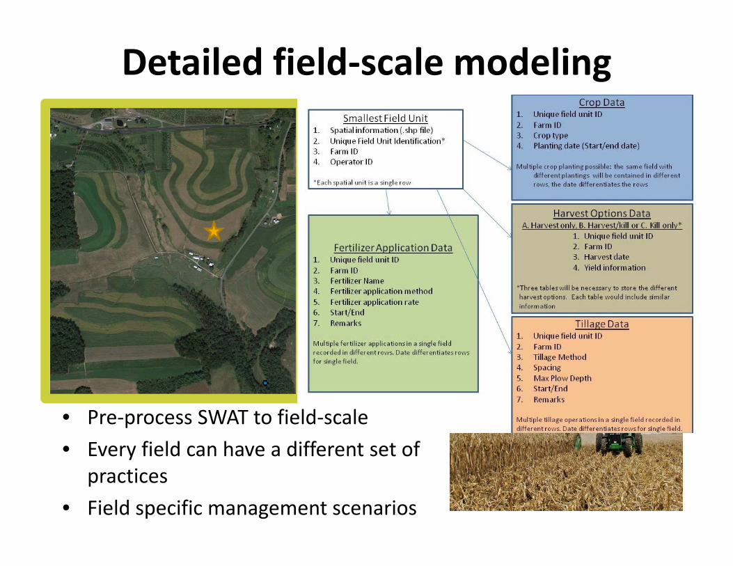
Detailed field‐scale modeling
https://i.ytimg.com/vi/wx0SJM7FeEc/mqdefault.jpg
http://www.extension.org/sites/default/files/w/4/4a/Spreading_manure.jpg
• Pre‐process SWAT to field‐scale• Every field can have a different set of
practices• Field specific management scenarios
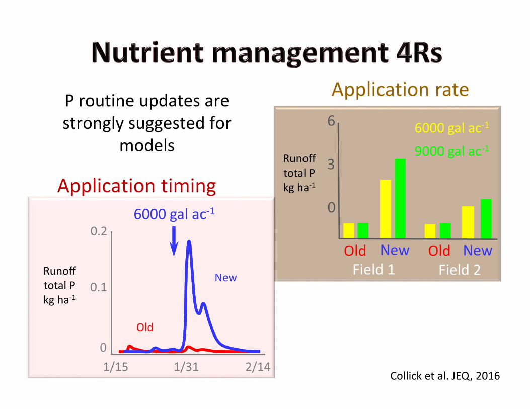
Application rate
Collick et al. JEQ, 2016
6000 gal ac‐1
9000 gal ac‐1
NewOld NewOld
6
3
0
Runoff total Pkg ha‐1
New
Old
Runoff total Pkg ha‐1
1/15 1/31 2/14
0.1
0
0.26000 gal ac‐1
Field 1 Field 2
P routine updates are strongly suggested for
models
Application timing

0.00
0.25
0.50
0.75
1.00
1/1/2010 2/20/2010 4/11/2010
0.0
1.0
2.0
3.0
4.0
1/1/2010 2/20/2010 4/11/2010
01020304050
MeasuredOldNew
No manure applied
Poultry litter applied, January (2 tons ac‐1)
Runo
ff P, m
g L‐1
Rainfall, mm
Runo
ff P, m
g L‐1
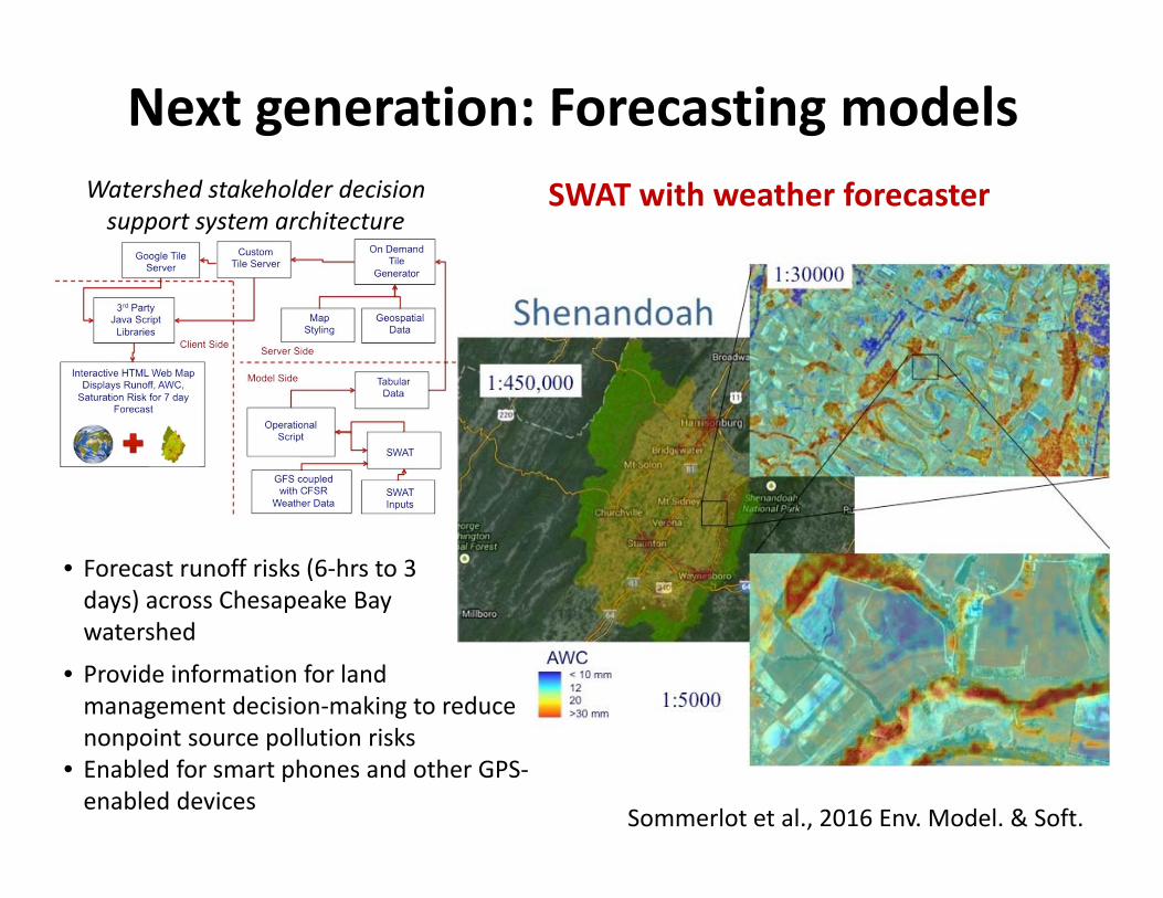
Next generation: Forecasting modelsSWAT with weather forecasterWatershed stakeholder decision
support system architecture
• Forecast runoff risks (6‐hrs to 3 days) across Chesapeake Bay watershed
• Provide information for land management decision‐making to reduce nonpoint source pollution risks
• Enabled for smart phones and other GPS‐enabled devices
Sommerlot et al., 2016 Env. Model. & Soft.
Our Solution
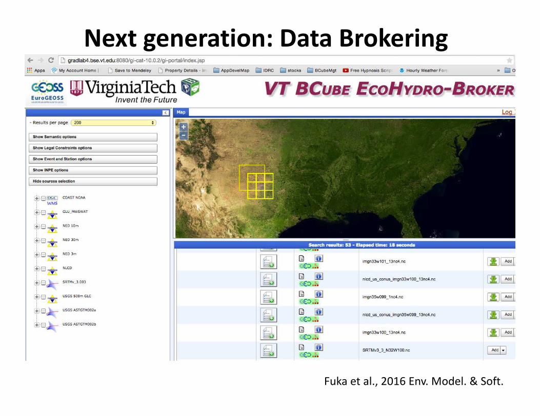
• Standardize data access and base datasets using a Broker
Next generation: Data Brokering
Fuka et al., 2016 Env. Model. & Soft.

Data Brokering in ArcSWAT

Lessons and Achievements
• Model Improvement: Better representation of critical source areas and nutrient transport
• Greater understanding of challenges/limitations in modeling P risk
• Model component comparisons (i.e., erosion) to pinpoint where changes are likely needed in P index
• Informed evaluations and modifications by nutrient management planners and stakeholders
• Expanded and enhanced collaborations between partners
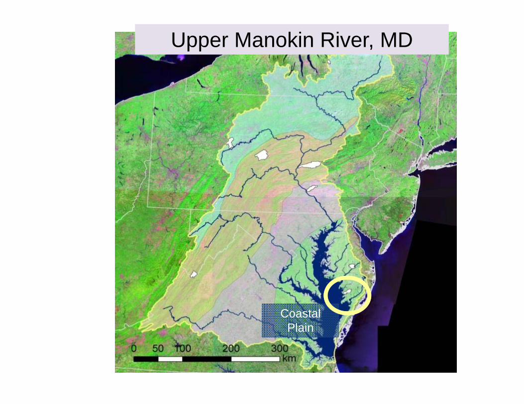
Upper Manokin River, MD
Coastal Plain
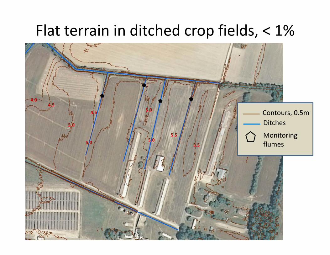
Flat terrain in ditched crop fields, < 1%
4.5
5.0 5.0
5.0
5.5
4.0 4.5
5.0
5.5
Ditches
Monitoring flumes
Contours, 0.5m
0 40 80 120 160 20020Meters
0 40 80 120 160 20020Meters
0 40 80 120 160 20020Meters
0 40 80 120 160 20020Meters
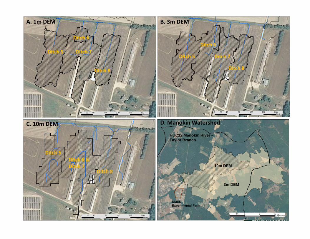
Figure : The delineations of the four ditches on the 1m LiDAR (A), 3m NED DEM (B) and 10m NED DEM (C). Only three drainage areas are apparent from the 10m DEM.
A. 1m DEM B. 3m DEM
C. 10m DEM
0 1 2 30.5Kilometers
'4
0 1 2 30.5Kilometers
HUC12 Manokin River –Taylor Branch
10m DEM
3m DEM
UMES Experimental Farm
D. Manokin Watershed
Ditch 5 Ditch 7
Ditch 6
Ditch 8
Ditch 5 Ditch 7
Ditch 6
Ditch 8
Ditch 5Ditch 6 & Ditch 7
Ditch 8
19
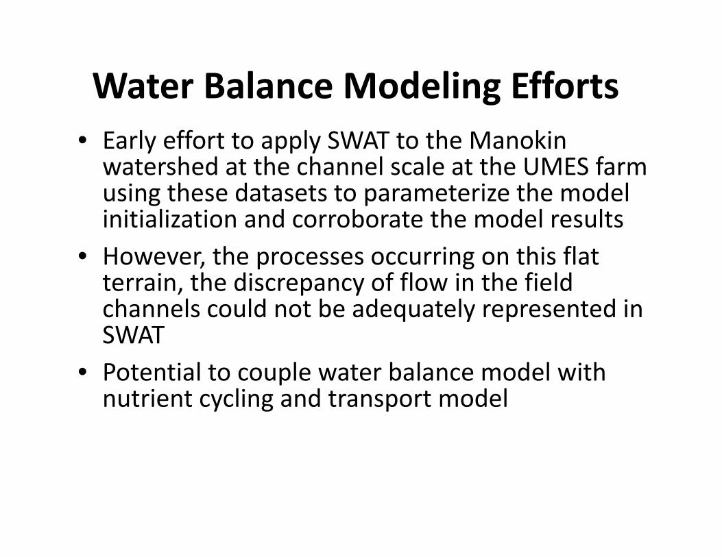
Water Balance Modeling Efforts• Early effort to apply SWAT to the Manokinwatershed at the channel scale at the UMES farm using these datasets to parameterize the model initialization and corroborate the model results
• However, the processes occurring on this flat terrain, the discrepancy of flow in the field channels could not be adequately represented in SWAT
• Potential to couple water balance model with nutrient cycling and transport model
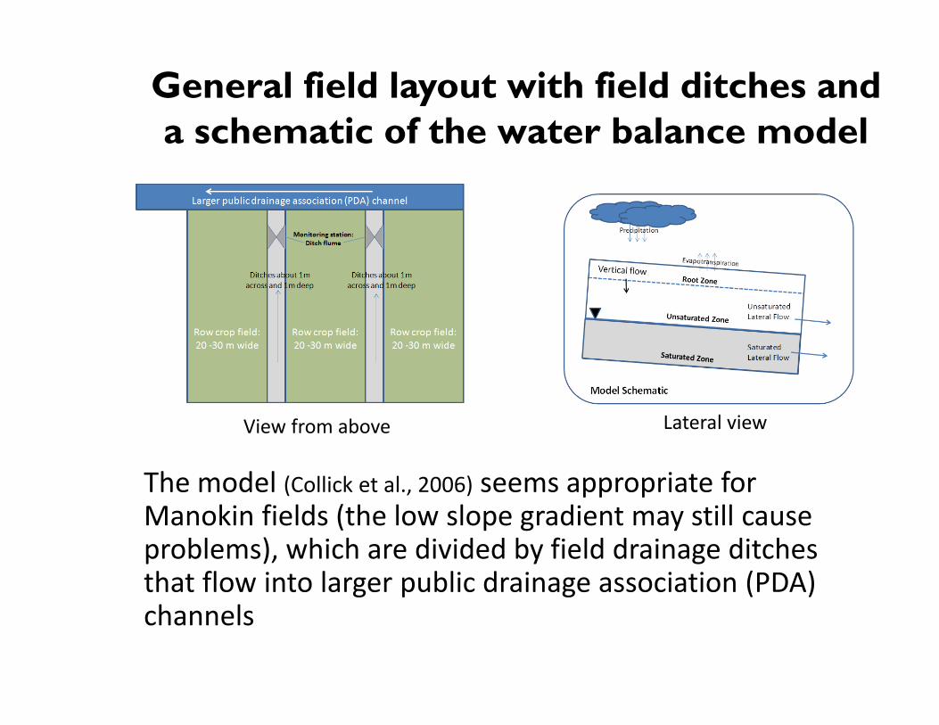
General field layout with field ditches and a schematic of the water balance model
View from above Lateral view
The model (Collick et al., 2006) seems appropriate for Manokin fields (the low slope gradient may still cause problems), which are divided by field drainage ditches that flow into larger public drainage association (PDA) channels
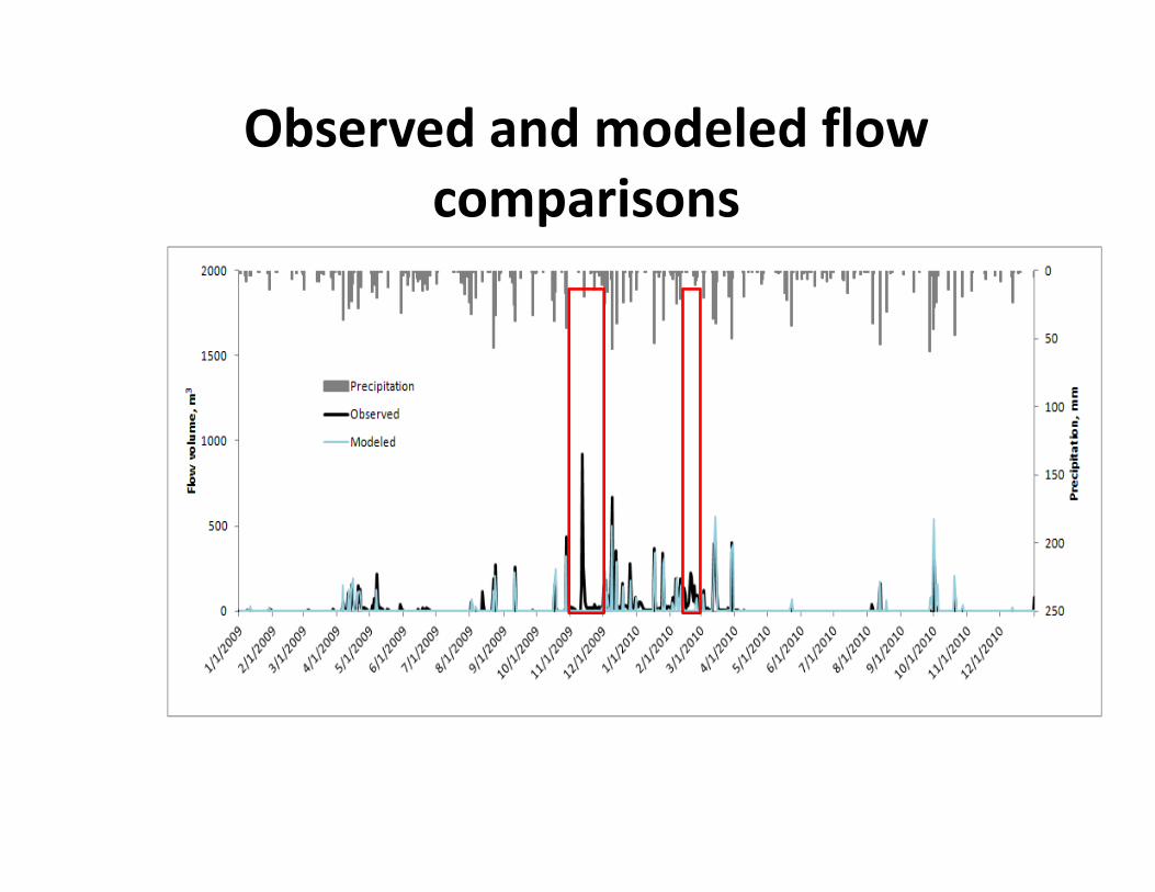
Observed and modeled flow comparisons
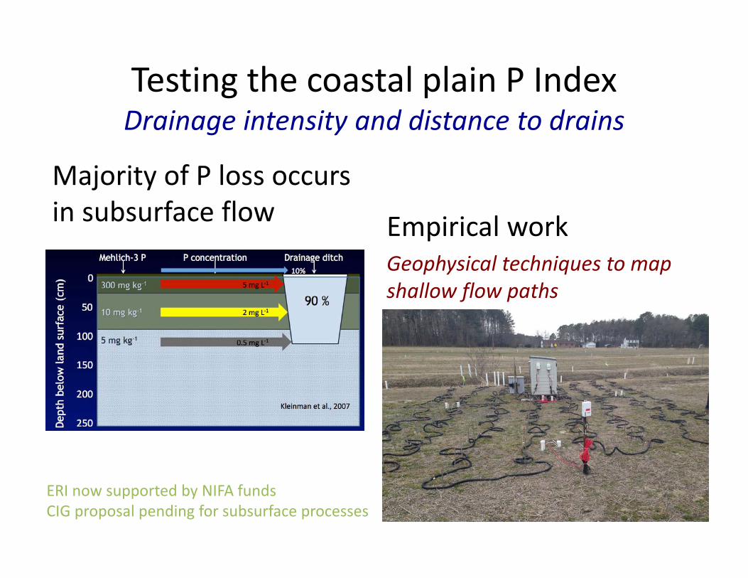
Testing the coastal plain P IndexDrainage intensity and distance to drains
Majority of P loss occurs in subsurface flow Empirical work
Geophysical techniques to map shallow flow paths
ERI now supported by NIFA fundsCIG proposal pending for subsurface processes

Factory Brook, NY
Allegheny Plateau
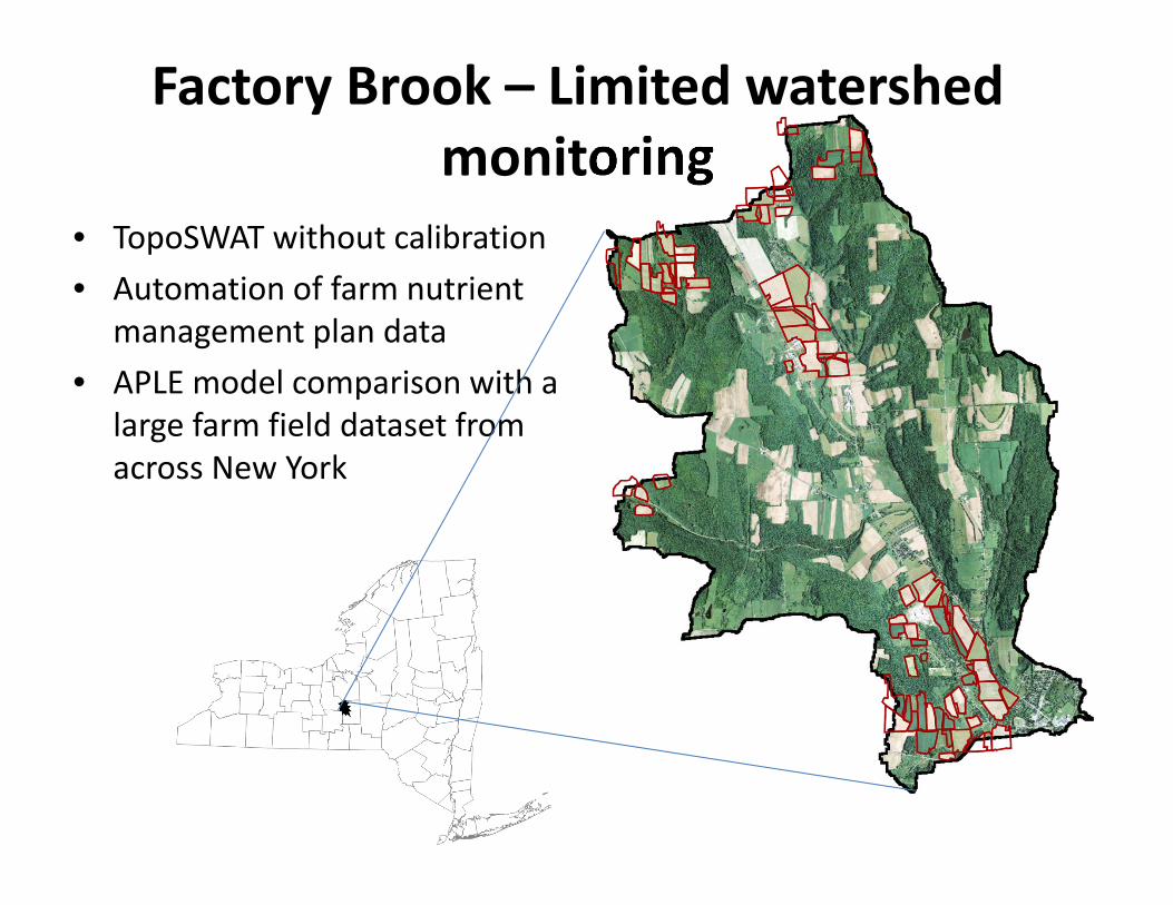
Factory Brook – Limited watershed monitoring
• TopoSWAT without calibration• Automation of farm nutrient
management plan data• APLE model comparison with a
large farm field dataset from across New York
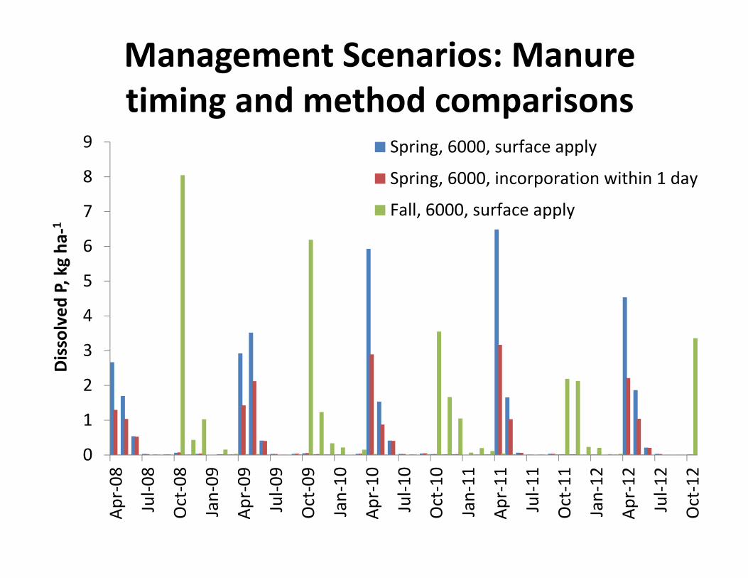
Management Scenarios: Manure timing and method comparisons
0
1
2
3
4
5
6
7
8
9Ap
r‐08
Jul‐0
8
Oct‐08
Jan‐09
Apr‐09
Jul‐0
9
Oct‐09
Jan‐10
Apr‐10
Jul‐1
0
Oct‐10
Jan‐11
Apr‐11
Jul‐1
1
Oct‐11
Jan‐12
Apr‐12
Jul‐1
2
Oct‐12
Dissolved
P, kg ha
‐1
Spring, 6000, surface apply
Spring, 6000, incorporation within 1 day
Fall, 6000, surface apply

Dissolved P loss
Particulate P loss
% %Comparison of application method, same amount of P applied
Spring, 6000, surface apply 100 100Spring, 6000, incorporation within 1 day 66 95Spring, 6000, injection 31 85Comparison of surface versus incorporation and injection, same N supply
Spring, 15500, surface apply 100 100Spring, 6000, incorporation within 1 day 23 52Spring, 6000, injection 11 47Comparison for cover crop use
Fall, 6000, surface apply 100 100Fall, 6000, surface apply + cover crop 110 81
Relative differences between methods to be compared to P index coefficients
Ketterings et al., 2016 in review, JEQ
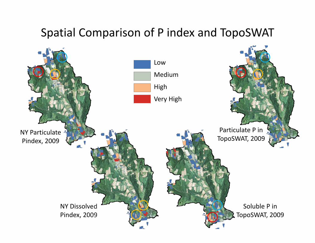
Spatial Comparison of P index and TopoSWAT
NY Dissolved Pindex, 2009
NY Particulate Pindex, 2009
Low
Medium
High
Very High
Soluble P in TopoSWAT, 2009
Particulate P in TopoSWAT, 2009
Lessons and Achievements
• Model Improvement: Better representation of critical source areas and nutrient transport
• Greater understanding of challenges/limitations in modeling P risk
• Model component comparisons (i.e., erosion) to pinpoint where changes are likely needed in P index
• Informed evaluations and modifications by nutrient management planners and stakeholders
• Expanded and enhanced collaborations between partners
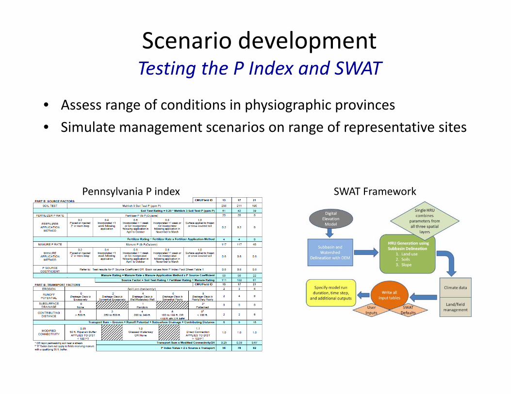
Scenario developmentTesting the P Index and SWAT
• Assess range of conditions in physiographic provinces• Simulate management scenarios on range of representative sites
SWAT FrameworkPennsylvania P index
.
. . .. . ....
. .
. . .. . ....
. .
. . .. . ....
. .
. . ... ... ..
..
...
. . .. . ....
. .
. . .. . ....
. .
. . .. . ....
. .
. . ... ... ..
..
...
. . .. . ....
. .
. . .. . ....
. .
. . .. . ....
. .
. . ... ... ..
..
..
.
. . .. . ....
. .
. . .. . ....
. .
. . .. . ....
. .
. . ... ... ..
..
..
.
. . .. . ....
. .
. . .. . ....
. .
. . .. . ....
. .
. . ... ... ..
..
...
. . .. . ....
. .
. . .. . ....
. .
. . .. . ....
. .
. . ... ... ..
..
...
. . .. . ....
. .
. . .. . ....
. .
. . .. . ....
. .
. . ... ... ..
..
..
.
. . .. . ....
. .
. . .. . ....
. .
. . .. . ....
. .
. . ... ... ..
..
..
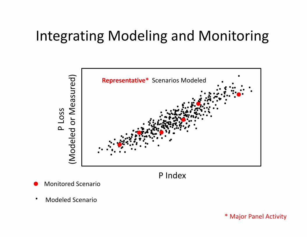
P Loss
(Mod
eled
or M
easured) Representative* Scenarios Modeled
Monitored Scenario
. Modeled Scenario
Integrating Modeling and Monitoring
* Major Panel Activity
P Index
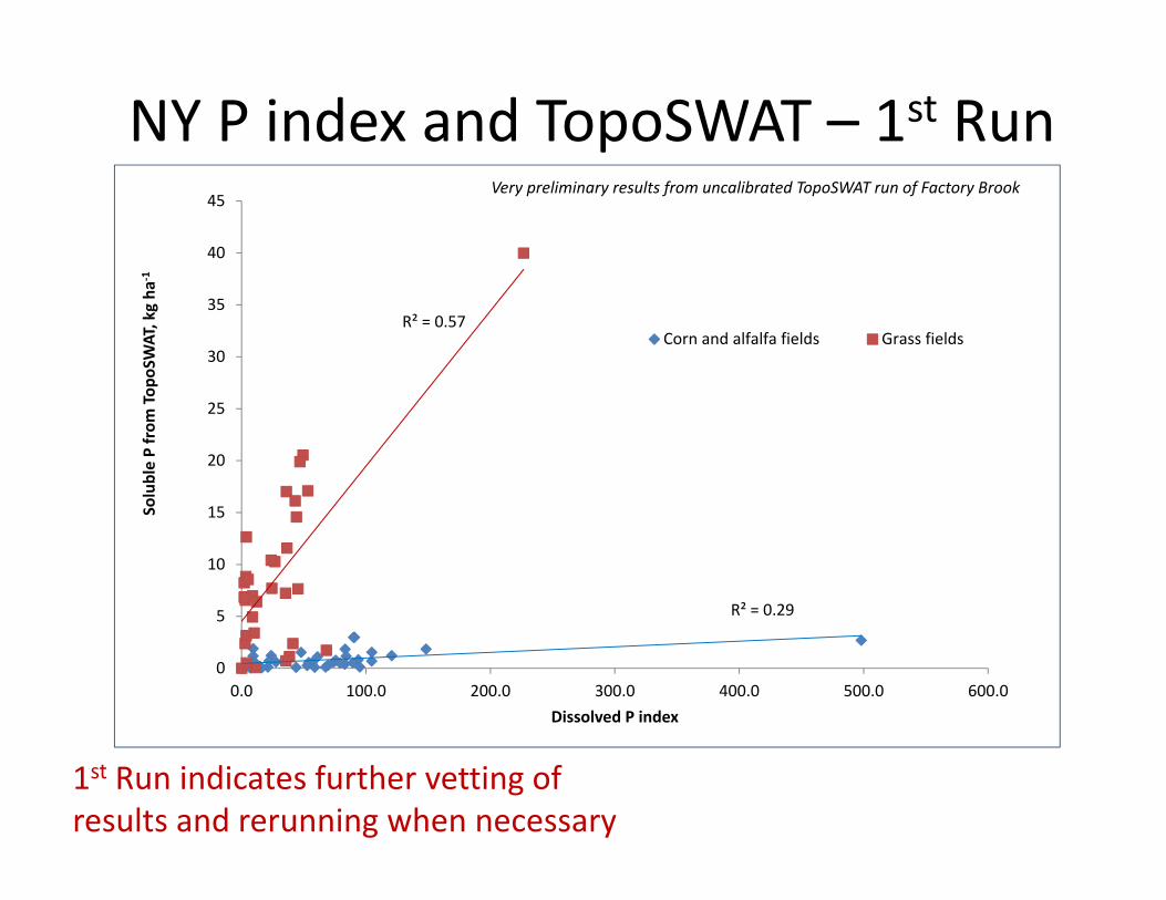
NY P index and TopoSWAT – 1st Run
R² = 0.29
R² = 0.57
0
5
10
15
20
25
30
35
40
45
0.0 100.0 200.0 300.0 400.0 500.0 600.0
Soluble P from
Top
oSWAT, kg ha
‐1
Dissolved P index
Corn and alfalfa fields Grass fields
Very preliminary results from uncalibrated TopoSWAT run of Factory Brook
1st Run indicates further vetting of results and rerunning when necessary
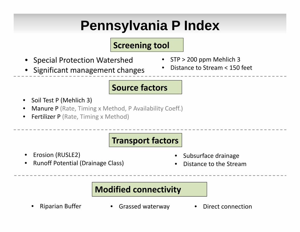
Pennsylvania P IndexScreening tool
• Special Protection Watershed• Significant management changes
• STP > 200 ppm Mehlich 3• Distance to Stream < 150 feet
Source factors• Soil Test P (Mehlich 3)• Manure P (Rate, Timing x Method, P Availability Coeff.)• Fertilizer P (Rate, Timing x Method)
Transport factors• Erosion (RUSLE2)• Runoff Potential (Drainage Class)
• Subsurface drainage• Distance to the Stream
Modified connectivity
• Riparian Buffer • Grassed waterway • Direct connection

SSURGO variables
SlopeDrainage classesSoil texture classDistance from
streamKsat
AWCTI classOM
USLE KMUKey

Developing reasonable scenariosWhat important conditions are missing in
our watersheds?Field management
Soils
Field delineation
Landuse
Topography
Watershed
Soil texture at variable distance
from stream

SSURGO data -- clay
% Clay

Lessons and Achievements
• Model Improvement: Better representation of critical source areas and nutrient transport
• Greater understanding of challenges/limitations in modeling P risk
• Model component comparisons (i.e., erosion) to pinpoint where changes are likely needed in P index
• Informed evaluations and modifications by nutrient management planners and stakeholders
• Expanded and enhanced collaborations between partners

Allegheny PlateauNew York and Pennsylvania
Ridge and Valley/PiedmontPennsylvania and West Virginia Coastal Plain
Delaware
Assess opinions regarding…– Current P Index factors (importance and reliability)– P Index modifications (boundaries and screening tool)
Evaluation and Revision of Phosphorus IndicesQuestionnaire for Nutrient Management Experts
Ketterings et al., 2016 in press, JSWCS

Lessons and Achievements
• Model Improvement: Better representation of critical source areas and nutrient transport
• Greater understanding of challenges/limitations in modeling P risk
• Model component comparisons (i.e., erosion) to pinpoint where changes are likely needed in P index
• Informed evaluations and modifications by nutrient management planners and stakeholders
• Expanded and enhanced collaborations between partners

Thank you! Questions??Amy S. Collick [email protected]


