
TECHNICAL UNIVERSITY OF CRETE
SCHOOL OF MINERAL RESOURCES ENGINEERING
PETROLEUM ENGINEERING MASTER COURSE
Master Thesis
“PERFORMANCE COMPARISON BETWEEN VARIOUS COMMERCIAL
SIMULATORS”
Author:
Aleksandar Mirkovic
Supervisor: Prof. Nikolaos Varotsis
Examination Committee:
Prof. Nikolaos Varotsis
Prof. Vassilis Gaganis
Prof. Nikolaos Pasadakis
Chania, 2018

A thesis submitted in fulfillment of the requirements for the
Master degree of Petroleum Engineering in the
School of Mineral Resources Engineering
Technical University of Crete
The MSc Program in Petroleum Engineering of the
Technical University of Crete, was attended and completed
by Mr. Aleksandar Mirkovic, due to the Hellenic Petroleum Group Scholarship award.

iv
Table of Contents
Table of Contents ........................................................................................................................... iv
List of Figures ................................................................................................................................ vi
List of Tables ................................................................................................................................. vi
Acknowledgements ...................................................................................................................... viii
Abstract .......................................................................................................................................... ix
1. The Function and Scope of Reservoir simulation ................................................................... 1
1.1 Introduction ...................................................................................................................... 1
1.2 Modeling approaches ....................................................................................................... 1
1.2.1 Analogical methods .................................................................................................. 1
1.2.2 Experimental methods .............................................................................................. 2
1.2.3 Mathematical methods .............................................................................................. 2
1.3 Application of Reservoir Simulation................................................................................ 4
1.4 Reservoir simulators classification................................................................................... 6
2. Model building ........................................................................................................................ 7
2.1 Geological model ............................................................................................................. 7
2.2 Flow models ..................................................................................................................... 9
2.3 Well models.................................................................................................................... 13
3. Numerical methods in reservoir simulation .......................................................................... 15
3.1 Review of finite difference ............................................................................................. 15
3.2 Application of finite difference on flow equation .......................................................... 17
3.2.1 Explicit finite difference approximation of the linear pressure equation ............... 17
3.2.2 Implicit finite difference approximation of the linear pressure equation ............... 19
3.2.3 IMPES (Implicit pressure explicit saturation) strategy ........................................... 21
4. Newton’s method .................................................................................................................. 22
5. Project strategy...................................................................................................................... 25
6. Models and results ................................................................................................................ 26
6.1 Reservoir description and fluid properties ..................................................................... 26

v
6.2 Validating models .......................................................................................................... 29
6.2.1 1D Single well model.............................................................................................. 29
6.2.2 1D Two wells model ............................................................................................... 30
6.3 Convergence study ......................................................................................................... 33
6.3.1 Eclipse convergence study ...................................................................................... 34
6.3.2 tNavigator convergence study................................................................................. 37
6.3.3 Comparison of converged models results .................................................................... 39
6.4 Runtimes comparison ..................................................................................................... 42
7. SPE 9 Model ......................................................................................................................... 45
8. Conclusion ............................................................................................................................ 50
9. Bibliography ......................................................................................................................... 51

vi
List of Figures
Figure 1.1 General form of MB equation ....................................................................................... 3
Figure 1.2 Grid illustration ............................................................................................................. 5
Figure 2.1 Grid example ................................................................................................................. 8
Figure 3.1 Finite difference illustration ........................................................................................ 15
Figure 3.2 Illustration of Pressure propagation in 1D ................................................................... 17
Figure 3.3 Illustration of explicit finite difference algorithm ....................................................... 19
Figure 4.1 Illustration of Newton method..................................................................................... 23
Figure 6.1 1D Single well model .................................................................................................. 29
Figure 6.2 Single well model reservoir pressure comparison ....................................................... 29
Figure 6.3 Single well model oil production rate comparison ...................................................... 30
Figure 6.4 Single well model cumulative oil production comparison .......................................... 30
Figure 6.5 1D Two well model ..................................................................................................... 31
Figure 6.6 1D Two well model oil production rate comparison ................................................... 31
Figure 6.7 1D Two well model water production rate comparison .............................................. 32
Figure 6.8 1D Two well model cumulative oil production comparison ....................................... 32
Figure 6.9 1D Two well model average reservoir pressure comparison ...................................... 32
Figure 6.10 Convergence study model ......................................................................................... 34
Figure 6.11 Oil production rate in Eclipse convergence study runs ............................................. 35
Figure 6.12 Water production rate in Eclipse convergence study runs ........................................ 35
Figure 6.13 Cumulative oil produced in Eclipse convergence study runs .................................... 36
Figure 6.14 Average reservoir pressure in Eclipse convergence study runs ................................ 36
Figure 6.15 Oil production rate in tNavigator convergence study runs ........................................ 37
Figure 6.16 Water production rate in tNavigator convergence study runs ................................... 38
Figure 6.17 Cumulative oil produced in tNavigator convergence study runs .............................. 38
Figure 6.18 Average reservoir pressure in tNavigator convergence study runs ........................... 39
Figure 6.19 Oil production rate comparison ................................................................................. 40
Figure 6.20 Water production rate comparison ............................................................................ 40
Figure 6.21 Cumulative oil produced comparison ........................................................................ 41
Figure 6.22 Average reservoir pressure comparison .................................................................... 41
Figure 6.23 Runtimes comparison ................................................................................................ 43
Figure 6.24 Time steps comparison .............................................................................................. 43
Figure 7.1 Model in 3D view (SPE 9) .......................................................................................... 45
Figure 7.3 Relative permeability (SPE 9) ..................................................................................... 46

vii
Figure 7.4 Capillary pressure (SPE 9) .......................................................................................... 46
Figure 7.5 Field oil production rate (SPE 9) ................................................................................. 48
Figure 7.6 Average reservoir pressure (SPE 9) ............................................................................ 48
List of Tables
Table 6.1 Reservoir Description ................................................................................................... 26
Table 6.2 PVDO............................................................................................................................ 27
Table 6.3 PVTW ........................................................................................................................... 27
Table 6.4 Densities........................................................................................................................ 27
Table 6.5 Relative permeability values ......................................................................................... 28
Table 6.6 Relative permeability curves ........................................................................................ 28
Table 6.7 Number of cells per model............................................................................................ 34
Table 6.8 Grid number of cells per model .................................................................................... 42
Table 6.9 Observed runtimes ........................................................................................................ 42
Table 7.1 Time steps (SPE 9) ....................................................................................................... 49

viii
Acknowledgements
I would like to express my sincere gratitude to my supervisor and members of committee for
their guidance and the scientific comments during this thesis.
Forever thankful to my family for all the support during this journey, we did it together.

ix
Abstract
This diploma thesis project will focus on the comparison of two black-oil simulation software.
The simulators under study are the widely known Eclipse 100 and the relatively new tNavigator
ones.
All commercial simulators available in the market are supposed to solve the same differential
equation problem using the same approach (finite volumes). However, the performance of them
might exhibit significant differences even treating exactly the same simulation problem. Those
differences might concern the computing time and/or the obtained results.
In this work we started with simple Cartesian reservoir models and compared their performance
against the simulators under study. Since the starting models were of low complexity and the
background formulation of both simulators was supposed to be the same the results in terms of
run time and simulators predictions should match. By verifying that it was shown that conditions
for fair comparison were established and the next comparison step was performed with models of
higher complexity. This allowed those fine differences in simulators to impact the prediction
outcome, as well as runtime of simulation. As the general comparison strategy of increasing the
model complexity is suitable for executing convergence study, this was done along the way. So,
became able to evaluate how these two simulators are dealing with error introduced by spatial
and temporal discretization as a part of numerical approximation of flow governing equations.
The output data consisting of key parameters (oil/water production rate, average reservoir
pressure and cumulative productions) for the respective model were compared along with CPU
runtimes.
By finalizing this study, a more solid judgement on performance of these two simulators on the
field of black-oil simulations has been built.

1.The Function and Scope of Reservoir simulation
1
1. The Function and Scope of Reservoir simulation
1.1 Introduction
The need for reservoir simulation rises from the necessity of having more accurate ways of
predicting reservoir performance under different operating conditions. Since the fact that all
petroleum engineering calculations are based on data which carries significant risk regarding
accuracy, which is usually magnified by engineering assumptions commonly needed for solving
specific problem. This is why, high accuracy risk associated with hydrocarbon recovery project
has to be associated and minimized. Factors contributing this risk include complexity of reservoir
heterogeneity, anisotropic rock properties, regional variations of fluid properties, complexity of
recovery mechanisms and limitations of predictive methods it selves.
The basic function of reservoir simulation is to predict future behavior of reservoir and
consequences of various reservoir management scenarios.
1.2 Modeling approaches
Common methods of forecasting reservoir performance generally can be divided into three
categories: analogical methods, experimental methods, and mathematical methods. Analogical
methods use properties of mature reservoirs that are either geographically or petrophysically
similar to the target reservoir to attempt to predict reservoir performance of a target reservoir.
Experimental methods measure physical properties in laboratory models and scale these results
to entire reservoir. Mathematical methods use equations which are formulating fluid flow in
porous media to predict reservoir performance. (Ertekin, 2001)
1.2.1 Analogical methods
In the early stages of field development, such as before drilling phase when there is very limited
or no available reservoir data, analogical methods are commonly used in order to predict
reservoir performance and perform economic analysis. In this method reservoirs in the same
geological basin with similar petrophysical properties are used to predict performance of target
reservoir. These methods can be used to estimate recovery factors, production rates, decline
1.The Function and Scope of Reservoir simulation
2
rates, drive mechanisms etc. Reliable results can be achieved when two similar reservoirs are
compared and similar development strategies are used. (Ertekin, 2001)
1.2.2 Experimental methods
Experimental methods are playing key role in understanding petroleum reservoirs. Compared to
analogical methods they are more often used and mainly in form of corefloods, sandpacks and
slim tube tests. Definitely the most commonly used method is coreflood experiment which is
generally run on linear cores (reservoir rock sample). The main aim of this experiment is to
determine reservoir properties such as porosity and permeability, establishing recovery
mechanism and EOR methods testing. (Ertekin, 2001)
1.2.3 Mathematical methods
Mathematical methods are nowadays most commonly used methods. This category includes:
material balance method, decline curve analysis, analytical (well test), statistical and reservoir
simulation method. Generally majority of these methods can be performed by hand calculation or
simple applications of graphical procedures, yet many software packages are available for
performing these tasks.
Material balance method or widely called tank model is a mathematical representation of
reservoir. Basic principle of this method is mass conservation principle, the mass in the reservoir
after production interval (pressure drop Dp) is equal to the mass initially in reservoir minus mass
produced during production interval plus the mass added to reservoir (injection of fluid or fluid
influx). The simplest way to visualize material balance is that if the measured surface volume of
oil, gas and water were returned to a reservoir at the reduced pressure, it must fit exactly into the
volume of the total fluid expansion plus the fluid influx. There are many forms of material
balance equations which are all derived from a single generalized form (Figure 1.1 General form
of MB equation).
The material balance equation and its many different forms have many uses including:
▪ Confirming the producing mechanism
▪ Estimating the fluid in place
▪ Estimating gas cap sizes
▪ Estimating water influx volumes

1.The Function and Scope of Reservoir simulation
3
▪ Identifying water influx model parameters
▪ Estimating producing indices
However material balance method is highly dependent on input data accuracy and meeting the
underlying assumptions. The material balance equation does not take in to account spatial
variations of rock and fluid properties, thermodynamics of fluid flow in porous media, well
positions and is very sensitive to inaccuracies in measured reservoir pressure. Beside of these,
significant drawback of this method is necessity of pressure drop, which very often could be
prevented by natural water influx or pressure maintenance methods.
Figure 1.1 General form of MB equation
Where:
▪ Gfgi, Nfoi, and W are the initial free gas, oil, and water in place, respectively
▪ Gp, Np, and Wp are the cumulative produced gas, oil, and water, respectively
▪ GI and WI are the cumulative injected gas and water respectively
▪ Eg, Eo, Ew, and Ef are the gas, oil, water, and rock (formation) expansivities
Analytical methods are based on exact solution of theoretically derived models. These models
usually fully represent physical description of process, but very often results in very complex
equations. Which in order to be solved analytically, simplifying assumptions have to be applied.
Although these assumptions are applied in order to mathematically solve these equations,
physics of the problem is preserved. Analytical methods are commonly used to determine effect
of various parameters on reservoir performance.
Statistical methods are using empirical correlations which are statistically derived from historical
data of past performances of numerous reservoirs in order to predict future performance of
others. Correlations are usually derived from mature reservoirs, and used in nearby new
reservoirs. There is wide choice of correlations available in the literature for almost all
1.The Function and Scope of Reservoir simulation
4
parameters regarding reservoir and fluid properties. Since this method is based on utilization of
regression on specific data set. The properties of reservoir under study should be in range of
initial regression data set, in order to avoid significant forecasting inaccuracies. Forecasting
errors with these techniques are often in range of 20 to 40%.
Reservoir simulation method, the usage of this method as a predictive tool nowadays is standard
in petroleum industry. Widespread acceptance of this method can be attributed to significant
improvement of computers, mainly regarding processing power and increased memory.
Equations which are describing fluid flow in porous media are highly nonlinear, because of that
analytical methods cannot be used and solutions must be obtained with numerical methods.
Numerical methods (approximate methods) in contrast to analytical give the values of pressure
and saturations only at discrete points in the reservoir. Discretization is the process of converting
partial differential equations in algebraic ones. Overall analytical method provides exact solution
of specific (simple) problem, where numerical method gives approximation of exact solution for
(complex) problem. The discretization process results in system of nonlinear algebraic equations.
Which in order to be solved has to be linearized. Once the equations are linearized one of linear
equations solving techniques can be used. Generally there are two categories of these methods:
direct and iterative methods.
The direct methods are mainly based on Gaussian elimination, and exact solution is obtained
after specific number of mathematical operations.
In iterative methods an initial estimate of solution is successively improved until it is reasonably
close to the exact solution. The number of mathematical operations is not fixed and it hardly
depends on initial estimate, and allowed tolerance (deviation from exact solution).
1.3 Application of Reservoir Simulation
Reservoir simulation is widely used tool for making decisions on the development of new fields,
the location of infill wells, and the implementation of enhanced recovery projects. And is
generally performed in following steps:
1. Defining objectives of the study. This is done in respect to available data and production
history. Defining objectives means setting goals of study, making strategy and defining
ranges of expected physically sound outcomes.
1.The Function and Scope of Reservoir simulation
5
2. Collecting and validating reservoir data. After objective of the study is defined, the next
step is reservoir data collecting. It is important that data is validated, and that it satisfies
specific needs for building a model. Incorporating additional not necessary data may lead
to overload in terms of longer CPU run time or issues with model convergence.
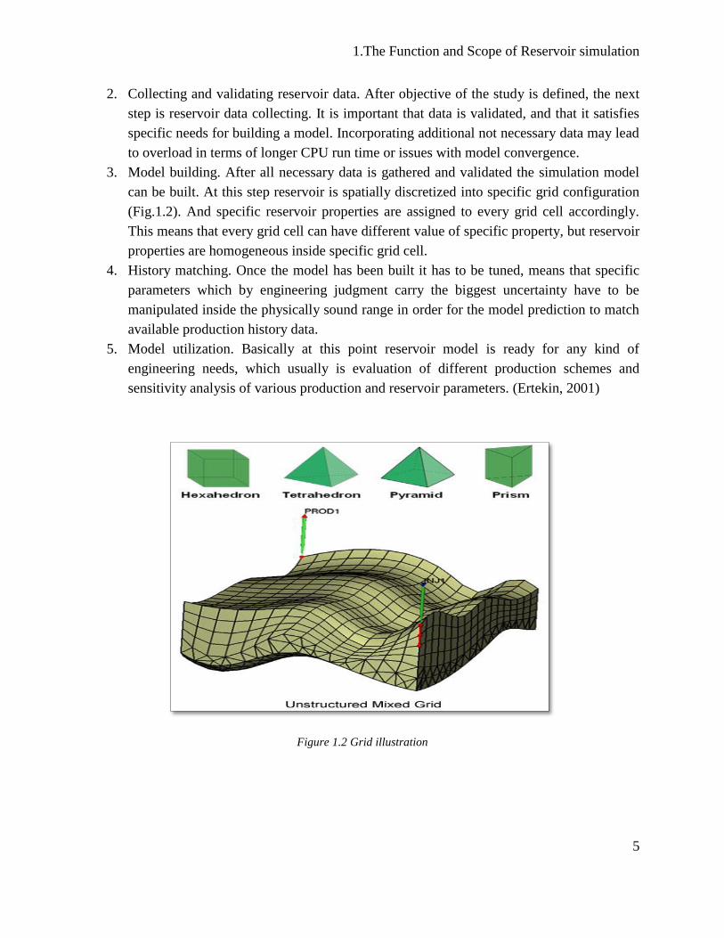
3. Model building. After all necessary data is gathered and validated the simulation model
can be built. At this step reservoir is spatially discretized into specific grid configuration
(Fig.1.2). And specific reservoir properties are assigned to every grid cell accordingly.
This means that every grid cell can have different value of specific property, but reservoir
properties are homogeneous inside specific grid cell.
4. History matching. Once the model has been built it has to be tuned, means that specific
parameters which by engineering judgment carry the biggest uncertainty have to be
manipulated inside the physically sound range in order for the model prediction to match
available production history data.
5. Model utilization. Basically at this point reservoir model is ready for any kind of
engineering needs, which usually is evaluation of different production schemes and
sensitivity analysis of various production and reservoir parameters. (Ertekin, 2001)
Figure 1.2 Grid illustration

1.The Function and Scope of Reservoir simulation
6
1.4 Reservoir simulators classification
The most common way of classifying reservoir simulators is based on type of reservoir and the
fluid simulated, as well as on recovery processes occurring in the subject reservoir. Reservoir
simulators can also be classified according to the coordinate system used and the number of
phases.
Classification based on reservoir and fluid type generally includes black-oil and compositional
reservoir simulators. Black oil simulators are used in situations where recovery processes are
insensitive to compositional changes in the reservoir fluid. Compositional simulators are used
when recovery processes are sensitive to compositional changes in the reservoir fluid. This
usually includes depletion of volatile-oil and gas-condensate reservoirs.
Classifications based on recovery processes include conventional-recovery, chemical-flood,
thermal-recovery and miscible-displacement simulators. Basically the natural drive recovery
mechanisms (gas cap drive, water drive, solution-gas drive and gravity drainage) can all be
modelled with black oil simulator. As well as secondary recovery mechanisms such as water or
gas injection, as long as mass transfer effect is negligible. When it comes to more complex
depletion mechanisms such as polymer or surfactant floods, there is a need for more advanced
simulators such as chemical-flooding simulators or thermal-simulators. These simulators use
energy-balance equation in addition to mass-balance equation. (Ertekin, 2001)
2.Model building
7
2. Model building
This project has been done by utilization of black-oil reservoir simulators. Therefore emphasis
was put on black-oil model configuration while other types of reservoir simulators will be briefly
mentioned.
Hydrocarbon resources are found within sedimentary rocks that have specific petrophysical
characteristics and as such are able to accommodate and transmit fluid. The fluid flow in porous
media actually occurs on a micrometer scale in the void space between the rock grains. While the
rock zones which carry hydrocarbons are often more than few meters thick and extend several
kilometers in the lateral directions. That explains why those rock formations are usually highly
heterogeneous in all directions, and what makes a flow in subsurface reservoirs a true mutliscale
problem. Therefore predicting reservoir performance has a large degree of uncertainty attached,
and usually one of main objectives of reservoir simulation is quantification of this uncertainty.
Reservoir simulation is the means by which, one uses a numerical model of the geological and
petrophysical characteristics of a hydrocarbon reservoir to analyze and predict fluid behavior in
the reservoir over time. In the general form, a reservoir model consists of:
1) Geological model in the form of a volumetric grid with cell/face properties that describes
the given porous rock formation
2) Flow model that describes fluid flow in porous media, usually given as a set of partial
differential equations
3) Well model that describes the fluid inflow into wellbore, fluid flow within the wellbore
and surface facilities.
2.1 Geological model
Description of a reservoir and its petrophysical parameters is usually done through a complex
workflow that involves processing data from knowledge of the geologic history of the
surrounding basin, seismic and electromagnetic surveys, study of geological analogues (bedrock
surface exposures), to rock samples extracted from exploration and production wells. All this
data presents input to the reservoir simulation in the form of volumetric grid. Each grid cell
provides petrophysical properties that are needed as input to the simulation model, primarily
2.Model building
8
porosity and permeability. Two petrophysic (Pengbo Lu, 2011) (Dake, 2013) (Reservoir
Engineering, 2013) (Ewing, 1983) (Chen, 2001)al properties which are fundamental for all
models. The rock porosity (Ф) is a dimensionless quantity that denotes the void volume fraction
of the medium available to be occupied by fluids. The permeability (K), is a measure of the
rock’s ability to transmit a single fluid under certain conditions.
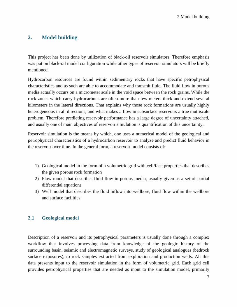
The industry standard is to use so-called stratigraphic grids that are designed to reflect that
reservoirs are usually formed through deposition of sediments and consist of stacks of
sedimentary beds with different solid particles and varying sizes that extend in the lateral
direction. Because of differences in deposition and compaction, the thickness and inclination of
each bed will vary in the lateral directions. For the purpose of reservoir simulation, fractures can
be considered as cracks or breakage in the rock, across which the layers in the rock have not
been displaced. Faults are fractures with displacement.
The most used format, so-called corner-pint grids, consists of a set of hexahedral cells that align
so that the cells can be numbered using logical I,J,K index. Each cell has eight logical corner
points. One or more corner-points may coincide, and cells that are logical neighbors don’t need
to have matching faces, which gives rise to unstructured connections. Stratigraphic grids will
usually have geometries that deviate far from regular hexahedra, which pose challenges for both
discretization methods and nonlinear solvers.
Figure 2.1 Grid example

2.Model building
9
2.2 Flow models
Second part of reservoir model is mathematical model that describes fluid flow. Respecting the
scope of this thesis project we will describe the most common models for isothermal flow.
Single-phase flow. The flow of a single fluid with density ρ through a porous medium is
described using the fundamental property of mass conservation.
(2.1)
Here, vector υ is the velocity and q denote a fluid source/sink term used to model wells. Velocity
is related to the fluid pressure p through and empirical relation named after French engineer
Henri Darcy:
(2.2)
Where K is permeability, µ fluid viscosity and g the gravity vector.
Two-phase flow. The pore space in reservoir is generally occupied by both hydrocarbons and
water. Water if often injected in reservoir as part of improved recovery strategy. If the fluids in
reservoir are immiscible and separated by a sharp interface, they are referred to as phases. A two-
phase system is commonly divided into a wetting and a non-wetting phase, given by the contact
angle between the solid surface and the fluid interface on the microscale. On the microscale, the
fluids are assumed to be present at the same location, and the volume fraction occupied by each
phase is called the saturation of that phase. Therefore, saturation for two-phase system of the
wetting and non-wetting phase sums to unity, So+Sw=1.
During the displacement, the ability of one phase to move is affected by the interaction with the
other phase at the pore scale. This effect is represented by the relative permeability Krα (α
=ω,n), which is a dimensionless scaling factor that depends on the saturation and modifies the
absolute permeability of wetting (ω) and non-wetting (n) phase to account for the rock’s reduced
ability to transmit each fluid in the presence of the other.
2.Model building
10
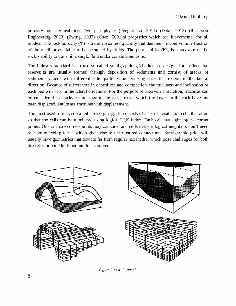
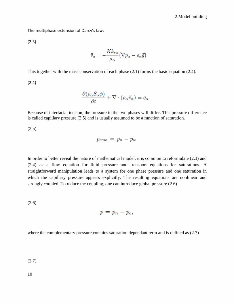
The multiphase extension of Darcy’s law: (2.3)
This together with the mass conservation of each phase (2.1) forms the basic equation (2.4).
(2.4)
Because of interfacial tension, the pressure in the two phases will differ. This pressure difference
is called capillary pressure (2.5) and is usually assumed to be a function of saturation.
(2.5)
In order to better reveal the nature of mathematical model, it is common to reformulate (2.3) and
(2.4) as a flow equation for fluid pressure and transport equations for saturations. A
straightforward manipulation leads to a system for one phase pressure and one saturation in
which the capillary pressure appears explicitly. The resulting equations are nonlinear and
strongly coupled. To reduce the coupling, one can introduce global pressure (2.6)
(2.6)
where the complementary pressure contains saturation dependant term and is defined as (2.7)
(2.7)

2.Model building
11
The dimensionless fractional-flow function (2.8) measures the fraction of the total flow that
contains the wetting phase and is defined from the phase mobilities (2.9).
(2.8)
(2.9)
In the incompressible and immiscible case, (2.3) and (2.4) can now be written as so called
fractional form which consists of an elliptic pressure equation (2.10)
(2.10)
for the pressure and the total velocity and a parabolic saturation equation (2.11) for the saturation
Sω of the wetting phase.
(2.11)
The capillary pressure can often be neglected in which case (2.11) becomes hyperbolic.
2.Model building
12
To solve the system (2.10) and (2.11) numerically, it is common to use sequential solution
procedure. First (2.10) is solved to determine the pressure and velocity, which are then held fixed
while advancing the saturation at time step dt, and so on.
The black-oil model is the most common used model within reservoir simulation. The model
uses a simple PVT description in which the hydrocarbon chemical species are lumped together to
form two components at surface conditions, a heavy hydrocarbon component called “oil” and
light hydrocarbon component called “gas”, for which the chemical composition remains constant
for all times. At reservoir conditions, the gas component may be partially or completely
dissolved in the oil phase, forming one or two phases (liquid and vapour) that do not dissolve in
the water phase. In more general models hydrocarbons are allowed to be dissolved in water
phase, and the water component may be dissolved in two hydrocarbon phases.
The black-oil model is often formulated as conservation of volumes at standard conditions, by
introducing formation volume factors (2.12), (Vα and Vαs are volumes occupied by a bulk of
component α at reservoir and surface conditions). That result in equations (2.13) and (2.14).
(2.12)
(2.13)
(2.14)
2.Model building
13
Commercial simulators typically use a fully implicit discretization to solve the nonlinear system
(2.13), (2.14). However, there are also several sequential methods that vary in the choice of
primary unknowns and the manipulations, linearization, temporal and spatial discretization, and
the order in which these operations are applied to derive a set of discrete equations. (Chen, 2001)
2.3 Well models
Simply speaking the well is open hole (conduit) through which fluid can flow in and out of the
reservoir. Modern wells are usually cemented and then perforated along specific intervals.
Generally there are two types of wells. Production wells, that are designed to extract
hydrocarbons and injection wells that are designed for injection of fluid under pressure into
reservoir (usually water or gas). The production/injection of fluids is controlled through surface
facilities, but wells may also contain advanced down-hole control devices.
The main objective of well models is to accurately represent the inflow from reservoir in the
wellbore and provide equations that can be used to compute injection or production rates when
the flowing bottom hole pressure is known, or compute the pressure for a given well rate. When
the equations presented in previous chapter are discretized using a volumetric grid, the wellbore
pressure will be significantly different from the average pressure in the perforated grid block.
The diameter of the wellbore is small compared to the size of the block, which implies that large
pressure gradients appear in a small region inside the perforated blocks. Modelling injection and
production of fluids using point sources gives singularities in the flow field and is seldom used in
practice. Instead, one uses an analytical or semi-analytical solution of the form (2.15) to relate
the wellbore pressure Pwb to the numerically computed pressure Pb inside the perforated blocks.
(2.15)

2.Model building
14
Here, the well index WI accounts for the geometric characteristics of the well and the properties
of the surrounding rock.
The first and still the most used model was developed by Peaceman (2.16). Assuming steady
state radial flow and a 7-point finite difference discretization, the well index for an isotropic
medium with permeability K represented on Cartesian grid represented by (2.16).
(2.16)
(2.17)
Here, rw is the radius of the well and ro is the effective block radius at which the steady-state
flowing pressure equals the numerically computed block pressure. The Peaceman model has later
been extended to multiphase flows, anisotropic media, horizontal wells, non-square grids, and
other discretization schemes, as well as to incorporate gravity effects, changes in near-well
permeability (skin), and non-Darcy effect. More advanced models describe the flow inside the
wellbore and how this flow is coupled with surface controls and processing facilities.
3.Numerical methods in reservoir simulation
15
3. Numerical methods in reservoir simulation
The multi-phase flow equations for real systems are so complex that it is not possible to solve
them analytically. In practice these equations can only be solved numerically. The most
commonly applied numerical methods are based on finite difference approximations of the flow
equations. In this chapter we will briefly review these methods.
3.1 Review of finite difference
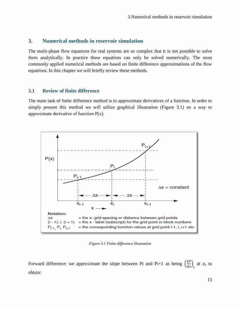
The main task of finite difference method is to approximate derivatives of a function. In order to
simply present this method we will utilize graphical illustration (Figure 3.1) on a way to
approximate derivative of function P(x).
Figure 3.1 Finite difference illustration
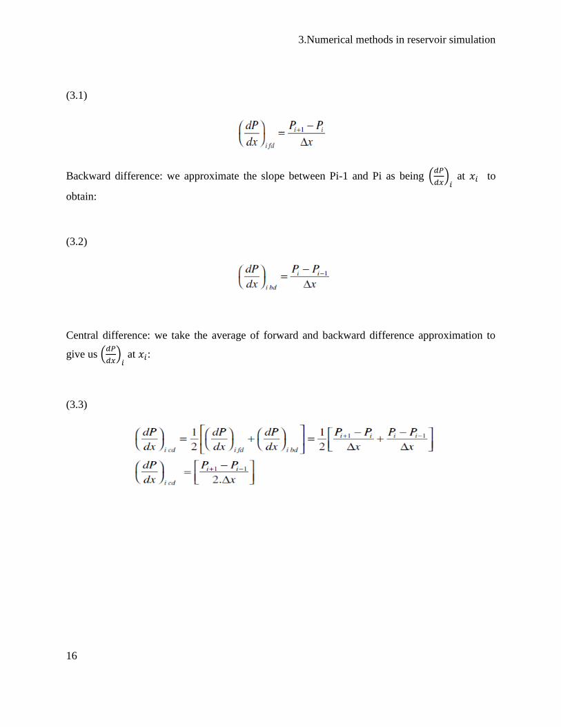
Forward difference: we approximate the slope between Pi and Pi+1 as being (𝑑𝑃
𝑑𝑥)
𝑖 at 𝑥𝑖 to
obtain:
3.Numerical methods in reservoir simulation
16
(3.1)
Backward difference: we approximate the slope between Pi-1 and Pi as being (𝑑𝑃
𝑑𝑥)
𝑖 at 𝑥𝑖 to
obtain:
(3.2)
Central difference: we take the average of forward and backward difference approximation to
give us (𝑑𝑃
𝑑𝑥)
𝑖 at 𝑥𝑖:
(3.3)
3.Numerical methods in reservoir simulation
17
3.2 Application of finite difference on flow equation
Due to the overall complexity of problem, in this chapter we will focus on explaining general
principle of PDE’s discretization on linear pressure equation in its simplest form, but satisfactory
for demonstration purpose.
3.2.1 Explicit finite difference approximation of the linear pressure equation
The flow equations are actually partial differential equations (PDE’s), with the unknowns, P(x,t)
and S(x,t), dependent on both space and time. As previously said, for this purpose we will utilize
simplified pressure equations (3.1), which is linear and has known analytical solutions for
various boundary conditions. However, this will be neglected and we will apply numerical
methods as an example of how to use finite differences to solve PDE’s numerically. As even
further simplification of this problem, we will assume term of hydraulic diffusivity (𝑘
𝑐µФ)
constant. This will result with equation (3.2).
(3.1)
(3.2)
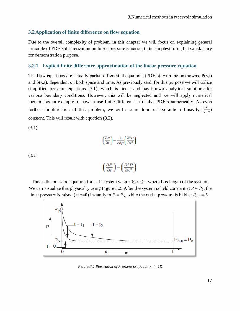
This is the pressure equation for a 1D system where 0≤ x ≤ L where L is length of the system.
We can visualize this physically using Figure 3.2. After the system is held constant at P = 𝑃0, the
inlet pressure is raised (at x=0) instantly to P = 𝑃𝑖𝑛 while the outlet pressure is held at 𝑃𝑜𝑢𝑡=𝑃0.
Figure 3.2 Illustration of Pressure propagation in 1D
3.Numerical methods in reservoir simulation
18
These pressures, 𝑃𝑖𝑛 and 𝑃𝑜𝑢𝑡 represent the constant pressure boundary conditions. This problem
is approached using finite difference as follows:
• discretize the x-direction by dividing into numerical grid of size ∆x;
• choose a time step, ∆t;
• use the following notation
n, time level
i, grid block label
𝑃𝑖𝑛, current (known) P at time level
𝑃𝑖𝑛+1, new (unknown) P at time level
• fix the boundary conditions
𝑃1= 𝑃𝑖𝑛 and 𝑃𝑜𝑢𝑡=𝑃0 which are fixed for all t.
• Apply finite difference for equation (3.2) using the above notation to obtain:
(3.3)
and
(3.4)
Equating the numerical finite difference approximations of each of the above derivatives as
required by the original PDE, equation (3.2) gives:
(3.5)
which by some simple manipulation can be expressed explicitly for 𝑃𝑖𝑛+1, the only unknown in
the above equation:
3.Numerical methods in reservoir simulation
19
(3.6)
Equation (3.6) provides algorithm for propagating solution of PDE equation (3.2), forward in
time from the given set of initial conditions.
The assumption that we made in order to obtain equation (3.4) was that the spatial derivative was
taken at the n (known) time level. This allowed us to develop explicit formula for 𝑃𝑖𝑛+1. This
method is therefore known as explicit finite difference method.
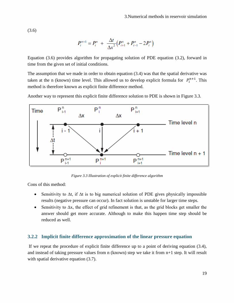
Another way to represent this explicit finite difference solution to PDE is shown in Figure 3.3.
Figure 3.3 Illustration of explicit finite difference algorithm
Cons of this method:
• Sensitivity to ∆t, if ∆t is to big numerical solution of PDE gives physically impossible
results (negative pressure can occur). In fact solution is unstable for larger time steps.
• Sensitivity to ∆x, the effect of grid refinement is that, as the grid blocks get smaller the
answer should get more accurate. Although to make this happen time step should be
reduced as well.
3.2.2 Implicit finite difference approximation of the linear pressure equation
If we repeat the procedure of explicit finite difference up to a point of deriving equation (3.4),
and instead of taking pressure values from n (known) step we take it from n+1 step. It will result
with spatial derivative equation (3.7).

3.Numerical methods in reservoir simulation
20
(3.7)
While the time derivative stays the same as (3.3).
As previously we can now equate (3.3) and (3.7) equation to obtain:
(3.8)
If we try and manipulate equation (3.8) in similar way as (3.5), we will easily realize that this
won’t be possible, because it appears that now we have three unknowns 𝑃𝑖−1𝑛+1 ,𝑃𝑖
𝑛+1 and𝑃𝑖+1𝑛+1.
Therefore, in order to solve this we have to rearrange equation (3.8) in following fashion:
(3.9)
.
Where all the unknowns are on the left-hand side and term on right hand side is known, since it
is from the n (known) time level. This expression gives us possibility to rewrite this equation as
follows:
(3.10)
.
Where:
𝑎𝑖−1= 1,
𝑎𝑖 = (2 +∆𝑥2
∆𝑡),
𝑎𝑖+1= 1 and 𝑏𝑖= −(∆𝑥2
∆𝑡) are all constants.
3.Numerical methods in reservoir simulation
21
The 𝑎𝑖 do not change throughout the calculation but the quantity 𝑏𝑖 is updated at each time step
as newly calculated 𝑃𝑛+1 is set as 𝑃𝑛. Solving this problem will always result in a system of
equation which for example of 20 grid points will give 18 equations, which combined with
boundary conditions can be solved. And it generally yields a sparse, tridiagonal matrix.
3.2.3 IMPES (Implicit pressure explicit saturation) strategy
The idea behind IMPES formulation lies somewhere between implicit and explicit formulation,
after we discretize the flow equations explicitly, we take constituents from next time step. In the
IMPES method we use time-lagged values of the saturation (from the known/previous step), the
pressure equation is linearized and can be solved implicitly for the pressure. After the latest
pressure value is obtained, we can solve for saturation explicitly, and repeat the process. That
makes IMPES an iterative process, which needs to be repeated until it converges. However,
IMPES has limitations in terms of time step size. If ∆t is to large, IMPES method may become
unstable and give unphysical results.
4.Newton’s method
22
4. Newton’s method
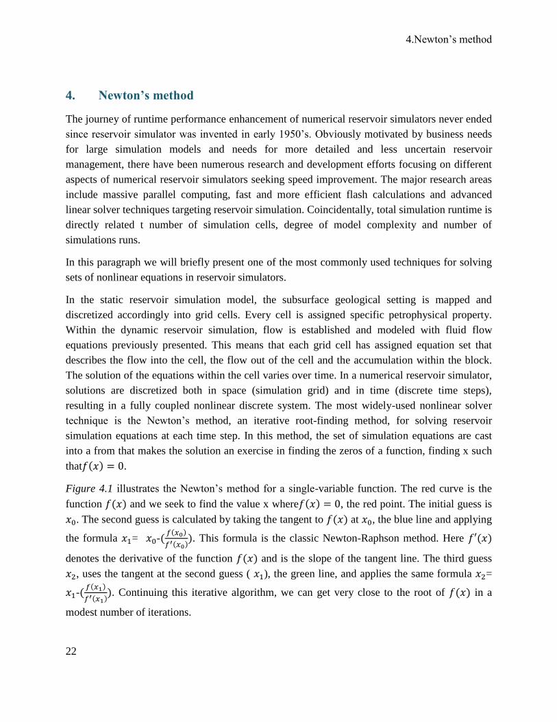
The journey of runtime performance enhancement of numerical reservoir simulators never ended
since reservoir simulator was invented in early 1950’s. Obviously motivated by business needs
for large simulation models and needs for more detailed and less uncertain reservoir
management, there have been numerous research and development efforts focusing on different
aspects of numerical reservoir simulators seeking speed improvement. The major research areas
include massive parallel computing, fast and more efficient flash calculations and advanced
linear solver techniques targeting reservoir simulation. Coincidentally, total simulation runtime is
directly related t number of simulation cells, degree of model complexity and number of
simulations runs.
In this paragraph we will briefly present one of the most commonly used techniques for solving
sets of nonlinear equations in reservoir simulators.
In the static reservoir simulation model, the subsurface geological setting is mapped and
discretized accordingly into grid cells. Every cell is assigned specific petrophysical property.
Within the dynamic reservoir simulation, flow is established and modeled with fluid flow
equations previously presented. This means that each grid cell has assigned equation set that
describes the flow into the cell, the flow out of the cell and the accumulation within the block.
The solution of the equations within the cell varies over time. In a numerical reservoir simulator,
solutions are discretized both in space (simulation grid) and in time (discrete time steps),
resulting in a fully coupled nonlinear discrete system. The most widely-used nonlinear solver
technique is the Newton’s method, an iterative root-finding method, for solving reservoir
simulation equations at each time step. In this method, the set of simulation equations are cast
into a from that makes the solution an exercise in finding the zeros of a function, finding x such
that𝑓(𝑥) = 0.
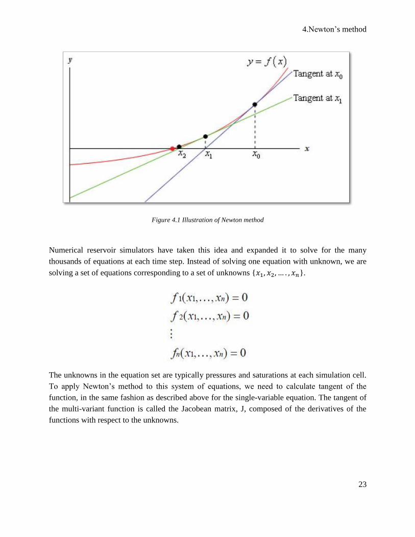
Figure 4.1 illustrates the Newton’s method for a single-variable function. The red curve is the
function 𝑓(𝑥) and we seek to find the value x where𝑓(𝑥) = 0, the red point. The initial guess is
𝑥0. The second guess is calculated by taking the tangent to 𝑓(𝑥) at 𝑥0, the blue line and applying
the formula 𝑥1= 𝑥0-(𝑓(𝑥0)
𝑓′(𝑥0)). This formula is the classic Newton-Raphson method. Here 𝑓′(𝑥)
denotes the derivative of the function 𝑓(𝑥) and is the slope of the tangent line. The third guess
𝑥2, uses the tangent at the second guess ( 𝑥1), the green line, and applies the same formula 𝑥2=
𝑥1-(𝑓(𝑥1)
𝑓′(𝑥1)). Continuing this iterative algorithm, we can get very close to the root of 𝑓(𝑥) in a
modest number of iterations.
4.Newton’s method
23
Figure 4.1 Illustration of Newton method
Numerical reservoir simulators have taken this idea and expanded it to solve for the many
thousands of equations at each time step. Instead of solving one equation with unknown, we are
solving a set of equations corresponding to a set of unknowns {𝑥1, 𝑥2, … . , 𝑥𝑛}.
The unknowns in the equation set are typically pressures and saturations at each simulation cell.
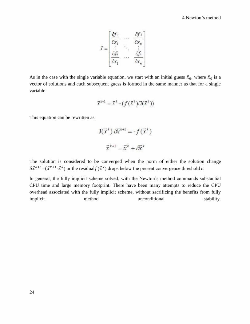
To apply Newton’s method to this system of equations, we need to calculate tangent of the
function, in the same fashion as described above for the single-variable equation. The tangent of
the multi-variant function is called the Jacobean matrix, J, composed of the derivatives of the
functions with respect to the unknowns.
4.Newton’s method
24
As in the case with the single variable equation, we start with an initial guess �⃗�0, where �⃗�0 is a
vector of solutions and each subsequent guess is formed in the same manner as that for a single
variable.
This equation can be rewritten as
The solution is considered to be converged when the norm of either the solution change
𝛿�⃗�𝑘+1=(�⃗�𝑘+1-�⃗�𝑘) or the residual𝑓(�⃗�𝑘) drops below the present convergence threshold ε.
In general, the fully implicit scheme solved, with the Newton’s method commands substantial
CPU time and large memory footprint. There have been many attempts to reduce the CPU
overhead associated with the fully implicit scheme, without sacrificing the benefits from fully
implicit method unconditional stability.

5.Project strategy
25
5. Project strategy
Usage of same personal computer for all comparative runs was a fundamental condition. Main
PC information are listed below:
Processor: Intel® Core™i7-7700HQ CPU @ 2.8GHz
RAM memory:16 GB
System: 64-bit Operating System, x64-based processor.
Primary goal was to ensure fair comparison environment, which was fulfilled by creating simple
Cartesian models (oil-water, low number of grid cells, uniform porosity and permeability
reservoir and single production well operating) in which depletion was driven by natural drive
mechanisms. Aim of this simulation runs was to obtain same output results due to low
complexity of model which is not allowing to any possible fine differences in simulator to take
place. Based on the fact that overall configuration of simulators is developed on same principles
with possibly only minor differences. If matching of output results from both simulators is
obtained, that was taken as a sign of fair comparison environment.
After ensuring that primary goal is achieved, the further strategy was to continue increasing
complexity of model. That was executed mainly by increasing number of grid blocks, and
introducing models with more complex recovery mechanisms such as waterflooding. During
whole study due to simplification and consistency reasons reservoir description including
geometry, petrophysical properties and fluid properties will remain same in all models beside of
SPE 9 Model. By increasing complexity of models, we expected those possible fine differences
in simulators to take place and express in a way of different simulation output. Emphasis was on
oil production rates, water production rate, average reservoir pressure and cumulative
production. As well at this point, we expected to observe noticeable CPU run time differences
due to higher complexity of models, which allowed efficiency of simulator solvers to affect run
time of simulations. According to this, briefly said we were increasing complexity of models,
while monitoring the simulation output and CPU run time of simulators. Following this work, we
performed brief model convergence (minimization of numerical error) study in both simulators
since the strategy of increasing model complexity by increasing number of cells is suitable for
this study.
While running the simulations we were continuously monitoring the previously mentioned
parameters, in order to ensure that all results were physically sound or in range of expected
values if fictive values of any of parameters were used in model itself, and that there are no
severe differences which may be caused by input model errors.

6.Models and results
26
After results were generated, the comparison plots of chosen output parameters were built for
every specific model in order to visualize eventual differences and CPU run times were
compared. Based on this we concluded with evaluation of chosen reservoir simulators.
6. Models and results
6.1 Reservoir description and fluid properties
In this chapter we will present reservoir description and fluid properties which will remain
constant through all models used in this study.
Geometrical and petrophysical description is provided in Table 6.1. As it can be seen reservoir is
dominantly extending in horizontal (X) direction with significantly thinner width (Y) and vertical
extent (Z). Permeability distribution is homogeneous in given directions. PVT properties of oil
are presented in Table 6.2, please note that gas density is provided in order to meet minimum
required data for input model despite of the fact that gas phase is not defined as existing phase.
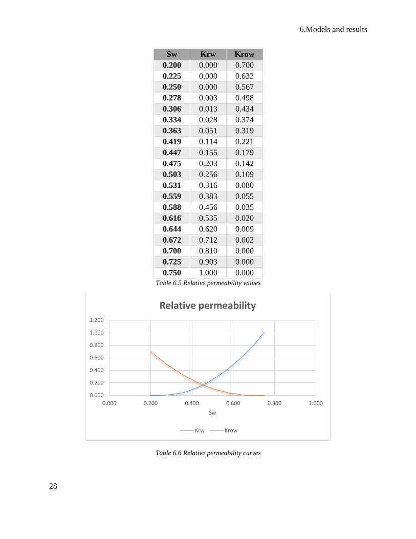
Oil could be characterized as light to medium heavy oil (Table 6.4 ). In order to acquire relative
permeability values Corey correlation model was built in CMG Simulation Builder (Table 6.5).
Reservoir description
Direction Dimension [ft]
X 4500
Y 150
Z 150
Depth [ft] 8000
Petrophysical properties
Porosity % 20
Direction Permeability [md]
X 200
Y 150
Z 50
Table 6.1 Reservoir Description

6.Models and results
27
Pressure [psi] Bo µ [cP]
2034 1.339 0.668869
2258 1.335 0.7
2515 1.33 0.75
2765 1.326 0.81
3015 1.322 0.86
3265 1.318 0.91
3515 1.314 1
3765 1.31 1.19
4015 1.307 1.197
4515 1.3 1.25
5015 1.294 1.3
Table 6.2 PVDO
PVTW
Pressure [psi] Bw Compressibility [1/psi] µ [cP]
4500 1.02 3.00E-06 0.8
Table 6.3 PVTW
Density [lbs/cft]
Oil 49
Water 63
Gas 0.01
Table 6.4 Densities
6.Models and results
28
Sw Krw Krow
0.200 0.000 0.700
0.225 0.000 0.632
0.250 0.000 0.567
0.278 0.003 0.498
0.306 0.013 0.434
0.334 0.028 0.374
0.363 0.051 0.319
0.419 0.114 0.221
0.447 0.155 0.179
0.475 0.203 0.142
0.503 0.256 0.109
0.531 0.316 0.080
0.559 0.383 0.055
0.588 0.456 0.035
0.616 0.535 0.020
0.644 0.620 0.009
0.672 0.712 0.002
0.700 0.810 0.000
0.725 0.903 0.000
0.750 1.000 0.000
Table 6.5 Relative permeability values
Table 6.6 Relative permeability curves
0.000
0.200
0.400
0.600
0.800
1.000
1.200
0.000 0.200 0.400 0.600 0.800 1.000
Sw
Relative permeability
Krw Krow

6.Models and results
29
6.2 Validating models
In this study we started with a simple 1D Cartesian model, in order to establish fair comparison
results by matching simulation output results. For this purpose we utilized two models with equal
number of grid cells (10) and same reservoir description (Table 6.1 Reservoir Description).The
difference in these two models is the depletion mechanism. In which, Model 1 has a single
production well and the depletion is driven by natural drive mechanisms, while Model 2 has one
production well and one injection well and as so the depletion is water driven.
6.2.1 1D Single well model
Number of grid cells 10x1x1. Well location 1, 1, 1 (Figure 6.2). Initial reservoir pressure 4500
psi. Well will be operating with constant bottomhole pressure (BHP) of 2000 psi.
Figure 6.1 1D Single well model
Figure 6.2 Single well model reservoir pressure comparison
0
1000
2000
3000
4000
5000
0 200 400 600 800 1000
Pre
ssu
re (
psi
a)
DAYS
Reservoir average pressure
tNavigator Eclipse

6.Models and results
30
Figure 6.3 Single well model oil production rate comparison
Figure 6.4 Single well model cumulative oil production comparison
As it can be seen from the obtained results, the peak of production rate was reached quickly and
it was followed with a rapid decay of production rate and finally the end of production. This can
be easily explained by the fact that depletion is done by limited natural drive (compaction drive).
The results from both of the simulators are perfectly matching.
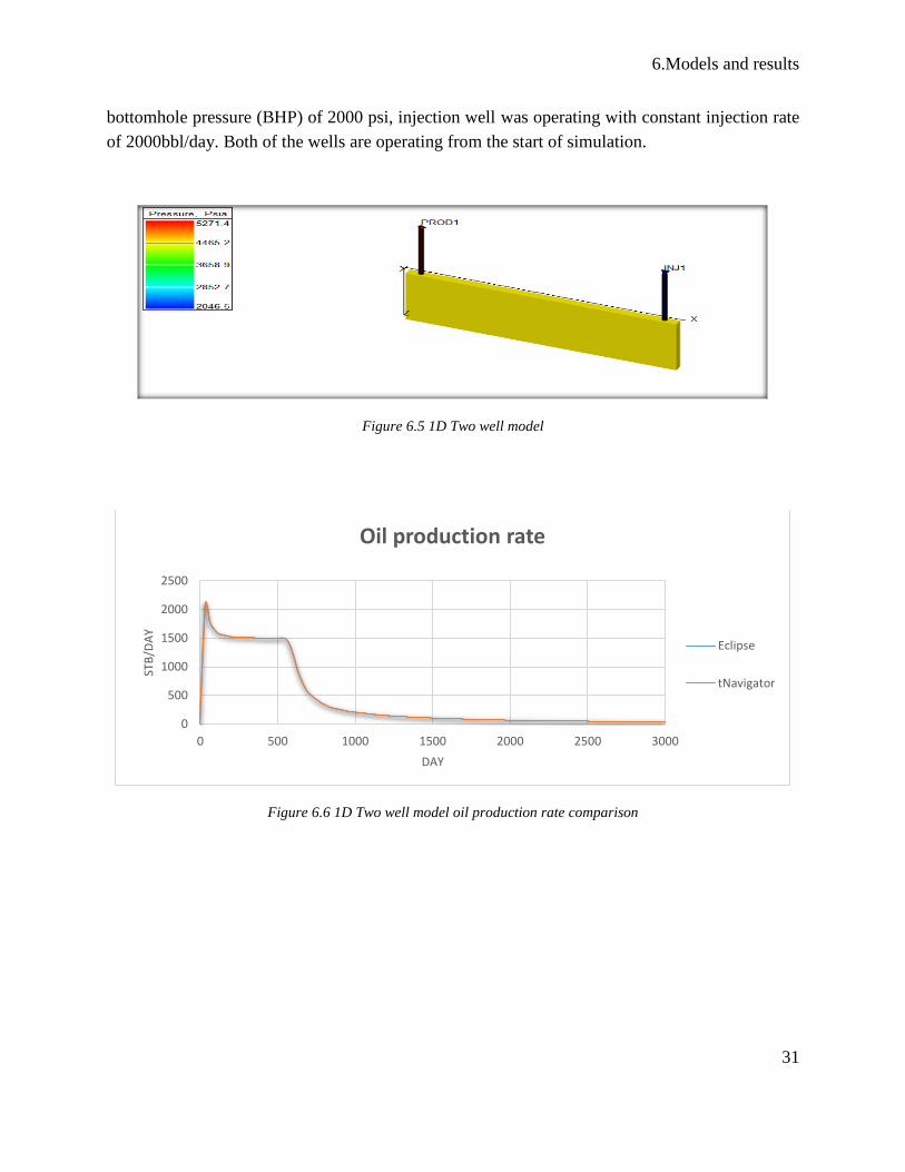
6.2.2 1D Two wells model
Number of grid cells 10x1x1. Production well location (1, 1, 1), injection well location (10, 1, 1).
(Figure 6.5). Initial reservoir pressure 4500 psi. Production well was operating with constant
0
500
1000
1500
0 200 400 600 800 1000
STB
/DA
Y
DAYS
Oil production rate
Eclipse
tNavigator
0
20000
40000
60000
80000
100000
120000
0 200 400 600 800 1000
STB
DAYS
Cumulative oil produced
Eclipse
tNavigator
6.Models and results
31
bottomhole pressure (BHP) of 2000 psi, injection well was operating with constant injection rate
of 2000bbl/day. Both of the wells are operating from the start of simulation.
Figure 6.5 1D Two well model
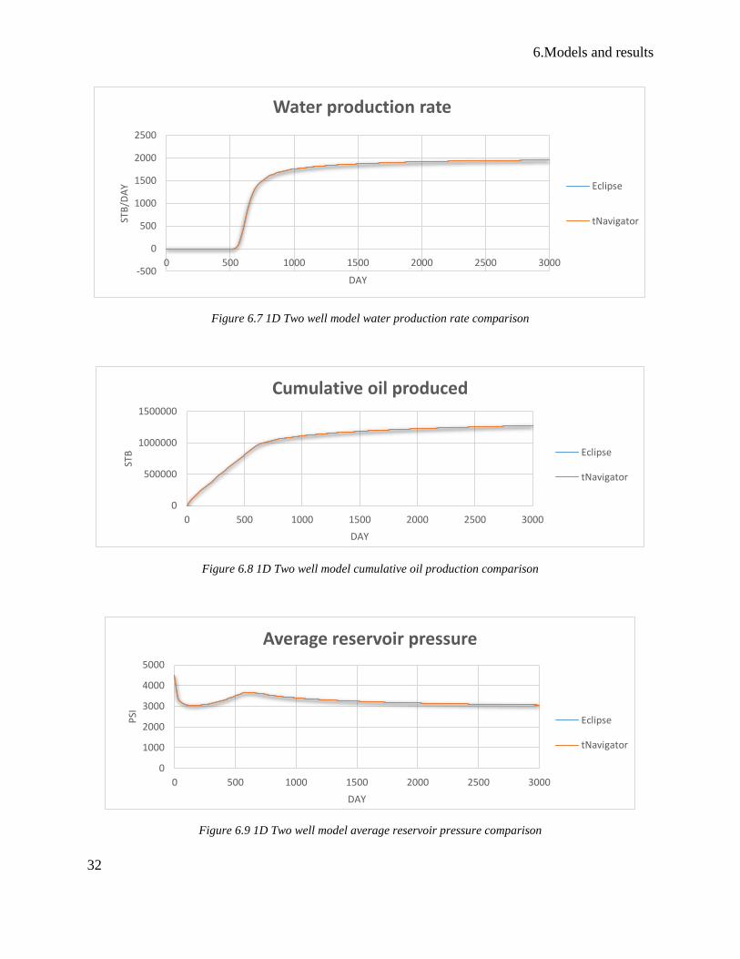
Figure 6.6 1D Two well model oil production rate comparison
0
500
1000
1500
2000
2500
0 500 1000 1500 2000 2500 3000
STB
/DA
Y
DAY
Oil production rate
Eclipse
tNavigator
6.Models and results
32
Figure 6.7 1D Two well model water production rate comparison
Figure 6.8 1D Two well model cumulative oil production comparison
Figure 6.9 1D Two well model average reservoir pressure comparison
-500
0
500
1000
1500
2000
2500
0 500 1000 1500 2000 2500 3000
STB
/DA
Y
DAY
Water production rate
Eclipse
tNavigator
0
500000
1000000
1500000
0 500 1000 1500 2000 2500 3000
STB
DAY
Cumulative oil produced
Eclipse
tNavigator
0
1000
2000
3000
4000
5000
0 500 1000 1500 2000 2500 3000
PSI
DAY
Average reservoir pressure
Eclipse
tNavigator
6.Models and results
33
As we can see from obtained results, we have peak of production rate quickly after the start of
production which is caused by natural drive mechanism and that is followed with rapid decay of
production rate until the waterflooding regime takes place. After that we can observe formation
of production plateau. Production plateau extends to the moment of water breakthrough, which
causes production well water cut to start growing., and further decay of oil production rate until
the moment when only flowing phase is water. All of that is as well depicted on average
reservoir pressure. We can see that perfect match of output results is achieved in both simulators
that we will take as a final evaluation of fairness in this comparison study and as approval to
continue with more complex models.
6.3 Convergence study
In this phase we were dealing with numerical dispersion introduced by spatial discretization, and
observed how these two simulators deal with similar problem. In this phase we started
monitoring CPU runtime of simulations, since complexity of models was gradually increasing as
a part of convergence study procedure. This procedure includes a multiple simulation runs,
where only variable will be number of grid cells. General principle is to start from low number of
grid cells and keep gradually increasing this variable, while the output results of simulation will
be approaching exact solution by every next update. During this study the only constrain was
runtime of simulation, which should stay in tolerable range (often decided by user). Practically it
is a balance between acceptable numerical error and satisfactory runtime duration. This study
provided as with suitable environment for CPU runtime comparison, because as previously
explained we had gradual growth of grid cells and model complexity.
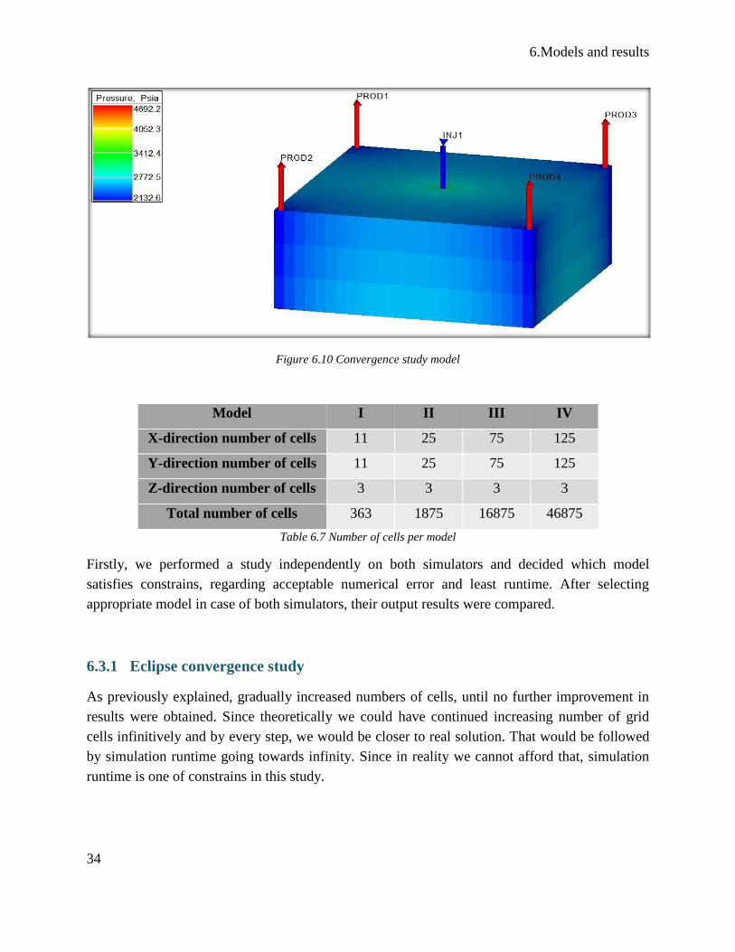
Model was built with previously presented reservoir and fluid properties (Chapter 6.1), with a
difference in reservoir dimensions (4500x4500x300 [ft]), OWC depth of 8350 [ft] and
waterflooding depletion mechanism. Including the 4 production wells which were always located
in the grid corners and 1 injection well located in the center of grid. Production wells were
producing with constant bottomhole pressure (2000 psi), while injection well was rate controlled
(50000 bbl/day). Injection rate has been given fictive value in order to keep average reservoir
pressure higher than production wells BHPs for whole period of simulation and avoid shutdown
of production wells.
Chosen grid dimensions will be presented in Table 6.7.
6.Models and results
34
Figure 6.10 Convergence study model
Model I II III IV
X-direction number of cells 11 25 75 125
Y-direction number of cells 11 25 75 125
Z-direction number of cells 3 3 3 3
Total number of cells 363 1875 16875 46875
Table 6.7 Number of cells per model
Firstly, we performed a study independently on both simulators and decided which model
satisfies constrains, regarding acceptable numerical error and least runtime. After selecting
appropriate model in case of both simulators, their output results were compared.
6.3.1 Eclipse convergence study
As previously explained, gradually increased numbers of cells, until no further improvement in
results were obtained. Since theoretically we could have continued increasing number of grid
cells infinitively and by every step, we would be closer to real solution. That would be followed
by simulation runtime going towards infinity. Since in reality we cannot afford that, simulation
runtime is one of constrains in this study.

6.Models and results
35
Figure 6.11 Oil production rate in Eclipse convergence study runs
Figure 6.12 Water production rate in Eclipse convergence study runs
0
20000
40000
60000
80000
100000
120000
140000
160000
180000
200000
0 1000 2000 3000 4000 5000 6000
STB
/DA
Y
DAY
Oil production rate (Eclipse)
11x11x3 25x25x3 75x75x3 125x125x3
0
10000
20000
30000
40000
50000
60000
0 1000 2000 3000 4000 5000 6000
STB
/DA
Y
DAY
Water production rate (Eclipse)
11x11x3 25x25x3 75x75x3 125x125x3

6.Models and results
36
Figure 6.13 Cumulative oil produced in Eclipse convergence study runs
Figure 6.14 Average reservoir pressure in Eclipse convergence study runs
0
10000
20000
30000
40000
50000
60000
70000
80000
90000
0 1000 2000 3000 4000 5000 6000
STB
DAY
Cumulative oil produced (Eclipse)
11x11x3 25x25x3 75x75x3 125x125x3
0
500
1000
1500
2000
2500
3000
3500
4000
4500
5000
0 1000 2000 3000 4000 5000 6000
Psi
a
DAY
Average reservoir pressure (Eclipse)
11x11x3 25x25x3 75x75x3 125x125x3

6.Models and results
37
By observing the obtained results, only slight improvement was achieved by increasing the
number of cells further than 75x75x3. But due to relatively short runtime of the larger
125x125x3 Model we will conclude that 125x125x3 Model converged, and take it as base model
in future comparison.
6.3.2 tNavigator convergence study
Procedure was done in the same manner as for Eclipse simulator.
Figure 6.15 Oil production rate in tNavigator convergence study runs
0
20000
40000
60000
80000
100000
120000
0 1000 2000 3000 4000 5000 6000
STB
/DA
Y
DAY
Oil production rate (tNavigator)
11x11x3 25x25x3 75x75x3 125x125x3
6.Models and results
38
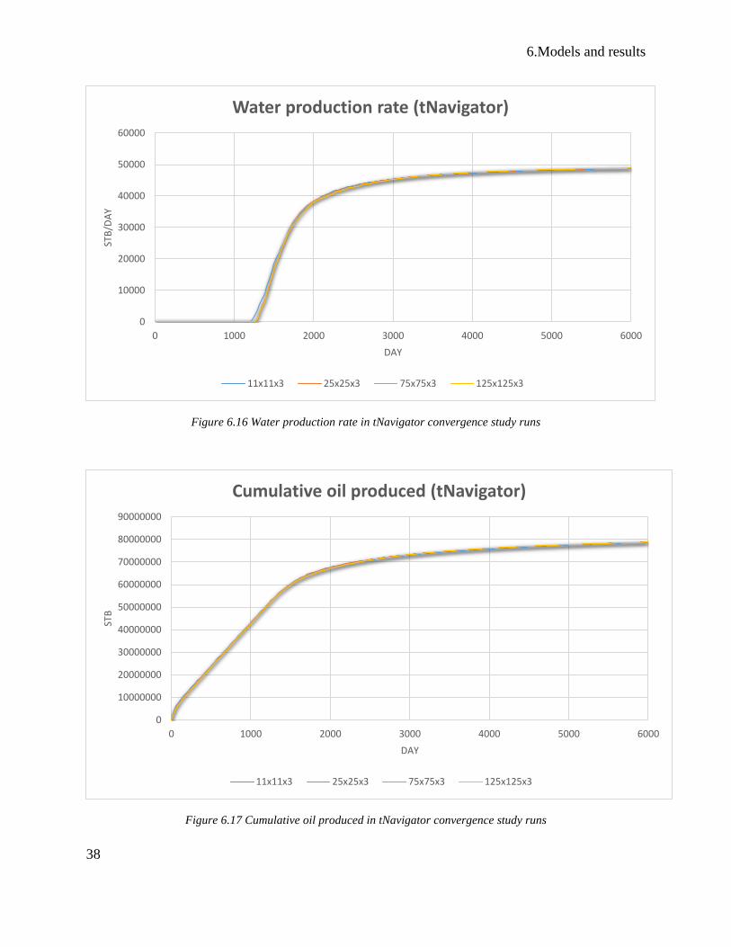
Figure 6.16 Water production rate in tNavigator convergence study runs
Figure 6.17 Cumulative oil produced in tNavigator convergence study runs
0
10000
20000
30000
40000
50000
60000
0 1000 2000 3000 4000 5000 6000
STB
/DA
Y
DAY
Water production rate (tNavigator)
11x11x3 25x25x3 75x75x3 125x125x3
0
10000000
20000000
30000000
40000000
50000000
60000000
70000000
80000000
90000000
0 1000 2000 3000 4000 5000 6000
STB
DAY
Cumulative oil produced (tNavigator)
11x11x3 25x25x3 75x75x3 125x125x3
6.Models and results
39
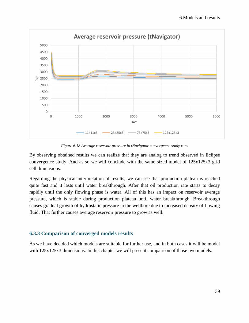
Figure 6.18 Average reservoir pressure in tNavigator convergence study runs
By observing obtained results we can realize that they are analog to trend observed in Eclipse
convergence study. And as so we will conclude with the same sized model of 125x125x3 grid
cell dimensions.
Regarding the physical interpretation of results, we can see that production plateau is reached
quite fast and it lasts until water breakthrough. After that oil production rate starts to decay
rapidly until the only flowing phase is water. All of this has an impact on reservoir average
pressure, which is stable during production plateau until water breakthrough. Breakthrough
causes gradual growth of hydrostatic pressure in the wellbore due to increased density of flowing
fluid. That further causes average reservoir pressure to grow as well.
6.3.3 Comparison of converged models results
As we have decided which models are suitable for further use, and in both cases it will be model
with 125x125x3 dimensions. In this chapter we will present comparison of those two models.
0
500
1000
1500
2000
2500
3000
3500
4000
4500
5000
0 1000 2000 3000 4000 5000 6000
Psi
a
DAY
Average reservoir pressure (tNavigator)
11x11x3 25x25x3 75x75x3 125x125x3
6.Models and results
40
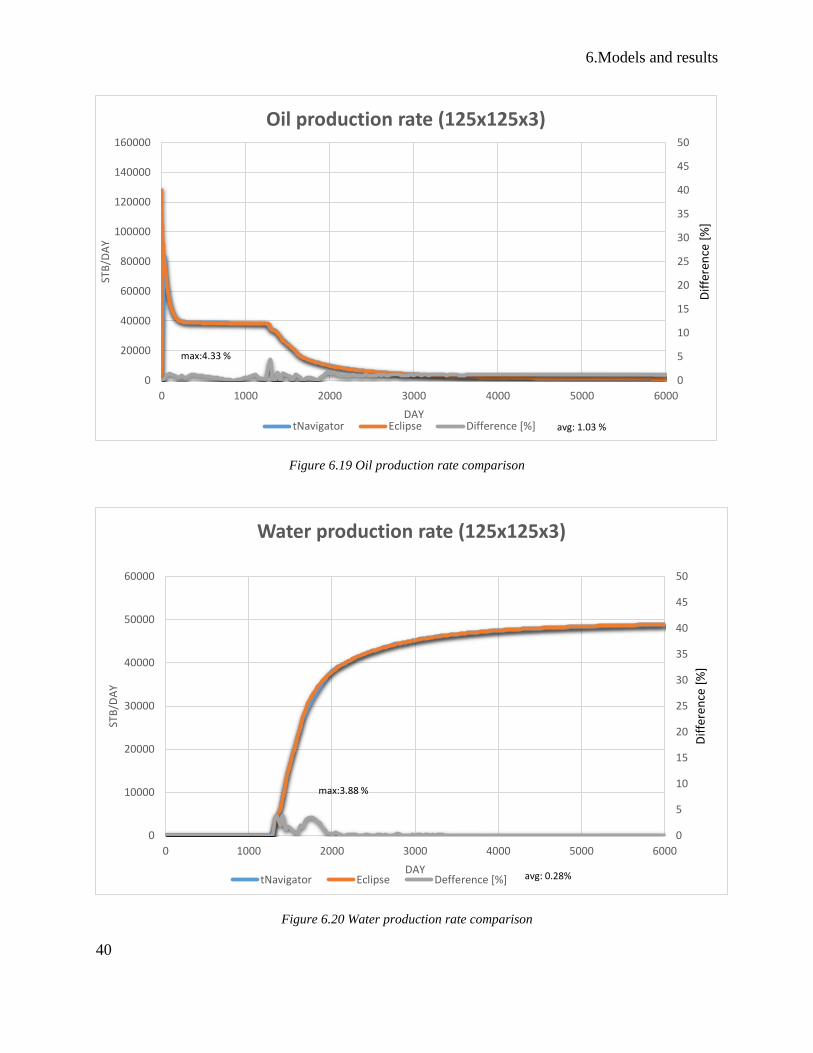
Figure 6.19 Oil production rate comparison
Figure 6.20 Water production rate comparison
0
5
10
15
20
25
30
35
40
45
50
0
20000
40000
60000
80000
100000
120000
140000
160000
0 1000 2000 3000 4000 5000 6000
Dif
fere
nce
[%
]
STB
/DA
Y
DAY
Oil production rate (125x125x3)
tNavigator Eclipse Difference [%]
max:4.33 %
avg: 1.03 %
0
5
10
15
20
25
30
35
40
45
50
0
10000
20000
30000
40000
50000
60000
0 1000 2000 3000 4000 5000 6000
Dif
fere
nce
[%
]
STB
/DA
Y
DAY
Water production rate (125x125x3)
tNavigator Eclipse Defference [%]
max:3.88 %
avg: 0.28%

6.Models and results
41
Figure 6.21 Cumulative oil produced comparison
Figure 6.22 Average reservoir pressure comparison
As we can see from presented figures, results from both simulators are matching. With minor
differences in output results ranging from 0 to 4.33% as the maximum value observed in oil
production rate results (Figure 6.19) due to respective time step. The average difference takes the
0
5
10
15
20
25
30
35
40
45
50
0
10000000
20000000
30000000
40000000
50000000
60000000
70000000
80000000
90000000
0 1000 2000 3000 4000 5000 6000
Dif
fere
nce
[%
]
STB
DAY
Cumulative oil produced (125x125x3)
tNavigator Eclipse Difference [%]
max: 0.74 %
avg: 0.11 %
0
5
10
15
20
25
30
35
40
0
500
1000
1500
2000
2500
3000
3500
4000
4500
5000
0 1000 2000 3000 4000 5000 6000
Dif
fere
nce
[%
]
Psi
a
DAY
Average reservoir pressure (125x125x3)
tNavigator Eclipse Difference [%]
max: 0.96 %
avg: 0.17 %
6.Models and results
42
maximum value of 1.03 % as well observed in oil production rate results, while lower average
differences are observed on the rest of results. These differences are mainly coming from
initialization steps or caused with sudden events such as water breakthrough.
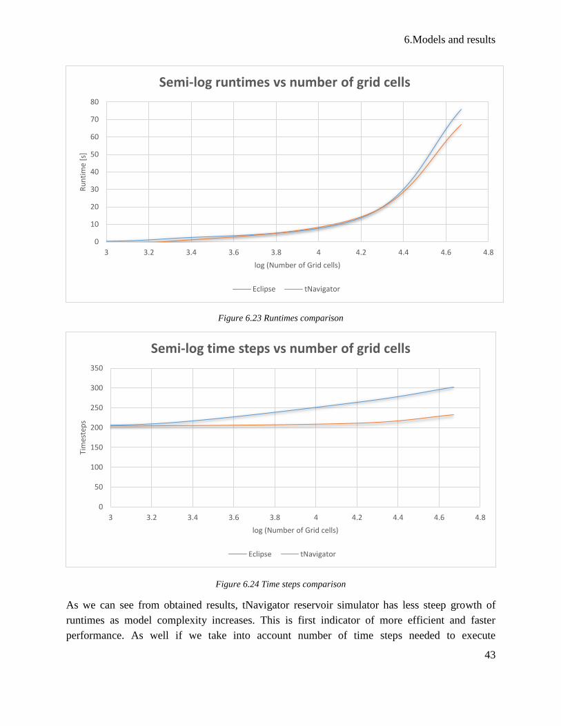
6.4 Runtimes comparison
Earlier in this study we have secured fair comparison environment, by matching the output of
both simulators on case of simple models. For which we believe the simulators should provide
same output due to low complexity of models. As well one more important condition was that all
runs were performed on same hardware, while all the background processes were terminated.
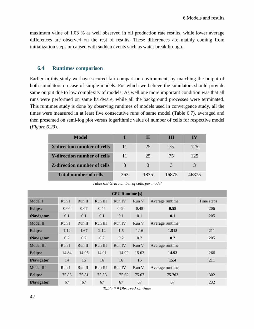
This runtimes study is done by observing runtimes of models used in convergence study, all the
times were measured in at least five consecutive runs of same model (Table 6.7), averaged and
then presented on semi-log plot versus logarithmic value of number of cells for respective model
(Figure 6.23).
Model I II III IV
X-direction number of cells 11 25 75 125
Y-direction number of cells 11 25 75 125
Z-direction number of cells 3 3 3 3
Total number of cells 363 1875 16875 46875
Table 6.8 Grid number of cells per model
CPU Runtime [s]
Model I Run I Run II Run III Run IV Run V Average runtime Time steps
Eclipse 0.66 0.67 0.45 0.64 0.48 0.58 206
tNavigator 0.1 0.1 0.1 0.1 0.1 0.1 205
Model II Run I Run II Run III Run IV Run V Average runtime
Eclipse 1.12 1.67 2.14 1.5 1.16 1.518 211
tNavigator 0.2 0.2 0.2 0.2 0.2 0.2 205
Model III Run I Run II Run III Run IV Run V Average runtime
Eclipse 14.84 14.95 14.91 14.92 15.03 14.93 266
tNavigator 14 15 16 16 16 15.4 211
Model III Run I Run II Run III Run IV Run V Average runtime
Eclipse 75.83 75.81 75.58 75.62 75.67 75.702 302
tNavigator 67 67 67 67 67 67 232
Table 6.9 Observed runtimes
6.Models and results
43
Figure 6.23 Runtimes comparison
Figure 6.24 Time steps comparison
As we can see from obtained results, tNavigator reservoir simulator has less steep growth of
runtimes as model complexity increases. This is first indicator of more efficient and faster
performance. As well if we take into account number of time steps needed to execute
0
10
20
30
40
50
60
70
80
3 3.2 3.4 3.6 3.8 4 4.2 4.4 4.6 4.8
Ru
nti
me
[s]
log (Number of Grid cells)
Semi-log runtimes vs number of grid cells
Eclipse tNavigator
0
50
100
150
200
250
300
350
3 3.2 3.4 3.6 3.8 4 4.2 4.4 4.6 4.8
Tim
este
ps
log (Number of Grid cells)
Semi-log time steps vs number of grid cells
Eclipse tNavigator

6.Models and results
44
calculations, we can see that Eclipse reservoir simulator needs significantly more time steps.
That can be taken as second indicator of efficiency, due to fact that simulator when unable to
converge it is forced to reduce the time step size (increase number of time steps). And that
directly affects the runtime of simulation.
7.SPE 9 Model
45
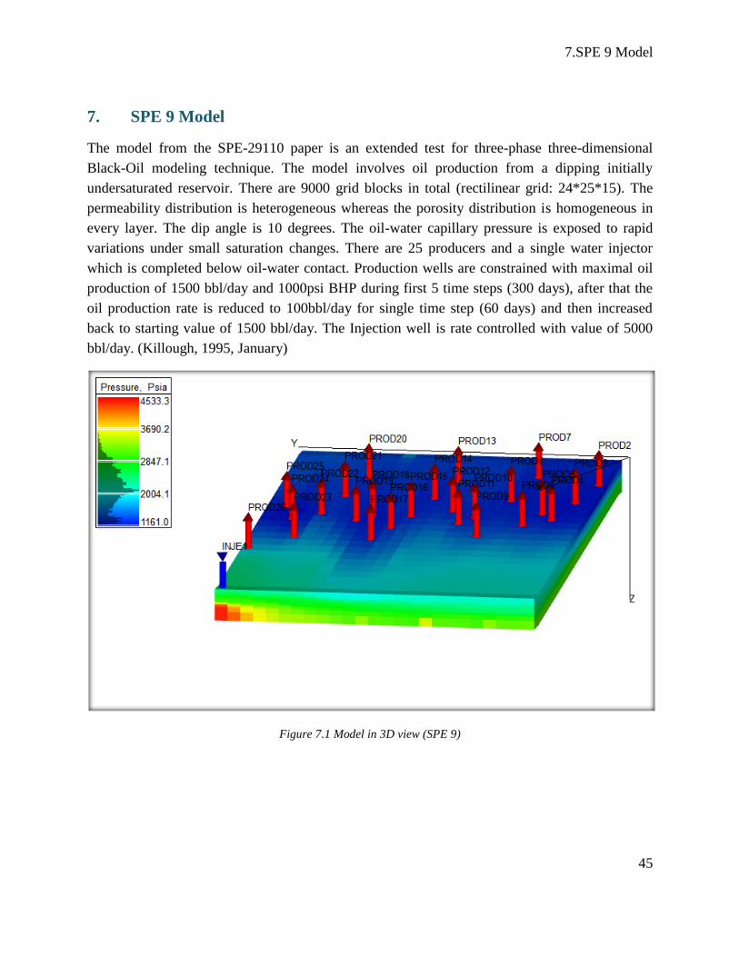
7. SPE 9 Model
The model from the SPE-29110 paper is an extended test for three-phase three-dimensional
Black-Oil modeling technique. The model involves oil production from a dipping initially
undersaturated reservoir. There are 9000 grid blocks in total (rectilinear grid: 24*25*15). The
permeability distribution is heterogeneous whereas the porosity distribution is homogeneous in
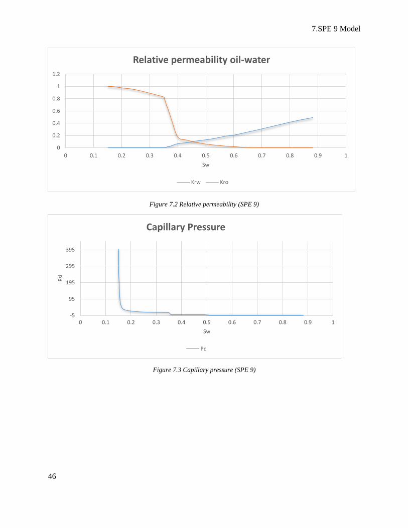
every layer. The dip angle is 10 degrees. The oil-water capillary pressure is exposed to rapid
variations under small saturation changes. There are 25 producers and a single water injector
which is completed below oil-water contact. Production wells are constrained with maximal oil
production of 1500 bbl/day and 1000psi BHP during first 5 time steps (300 days), after that the
oil production rate is reduced to 100bbl/day for single time step (60 days) and then increased
back to starting value of 1500 bbl/day. The Injection well is rate controlled with value of 5000
bbl/day. (Killough, 1995, January)
Figure 7.1 Model in 3D view (SPE 9)
7.SPE 9 Model
46
Figure 7.2 Relative permeability (SPE 9)
Figure 7.3 Capillary pressure (SPE 9)
0
0.2
0.4
0.6
0.8
1
1.2
0 0.1 0.2 0.3 0.4 0.5 0.6 0.7 0.8 0.9 1
Sw
Relative permeability oil-water
Krw Kro
-5
95
195
295
395
0 0.1 0.2 0.3 0.4 0.5 0.6 0.7 0.8 0.9 1
Psi
Sw
Capillary Pressure
Pc

7.SPE 9 Model
47
Pressure FVF,
rb/stb GOR,
Mscf/stb Viscosity,
cP
14.7 1 0 1.2
400 1.01 0.165 1.17
800 1.02 0.335 1.14
1200 1.03 0.5 1.11
1600 1.05 0.665 1.08
2000 1.06 0.828 1.06
2400 1.07 0.985 1.03
2800 1.08 1.13 1
3200 1.09 1.27 0.98
3600 1.11 1.39 0.95
4000 1.12 1.5 0.94
5000 1.11 1.5 0.94 Table 7.1 PVTO (SPE 9)
Oil, lbm/ft3
Water, lbm/ft3
Gas, lbm/ft3
44.98 63.01 0.0702
Table 7.2 Densities (SPE 9)
SPE 9 model will be used as final comparison between these two simulators. The emphasis will
be in oil production rate and reservoir average pressure.

7.SPE 9 Model
48
Figure 7.4 Field oil production rate (SPE 9)
Figure 7.5 Average reservoir pressure (SPE 9)
0
5
10
15
20
25
30
35
40
45
50
0
5000
10000
15000
20000
25000
30000
35000
40000
45000
50000
0 100 200 300 400 500 600 700 800 900
STB
/DA
Y
DAY
Field oil production rate
Eclipse tNavigator Difference [%] avg: 1.51 %
max: 4.25 %
0
5
10
15
20
25
30
35
40
45
50
0
500
1000
1500
2000
2500
3000
3500
4000
4500
5000
0 100 200 300 400 500 600 700 800 900
Psi
a
DAY
Average reservoir pressure
Eclipse tNavigator Difference [%] avg: 0.14 %
max: 0.29 %
7.SPE 9 Model
49
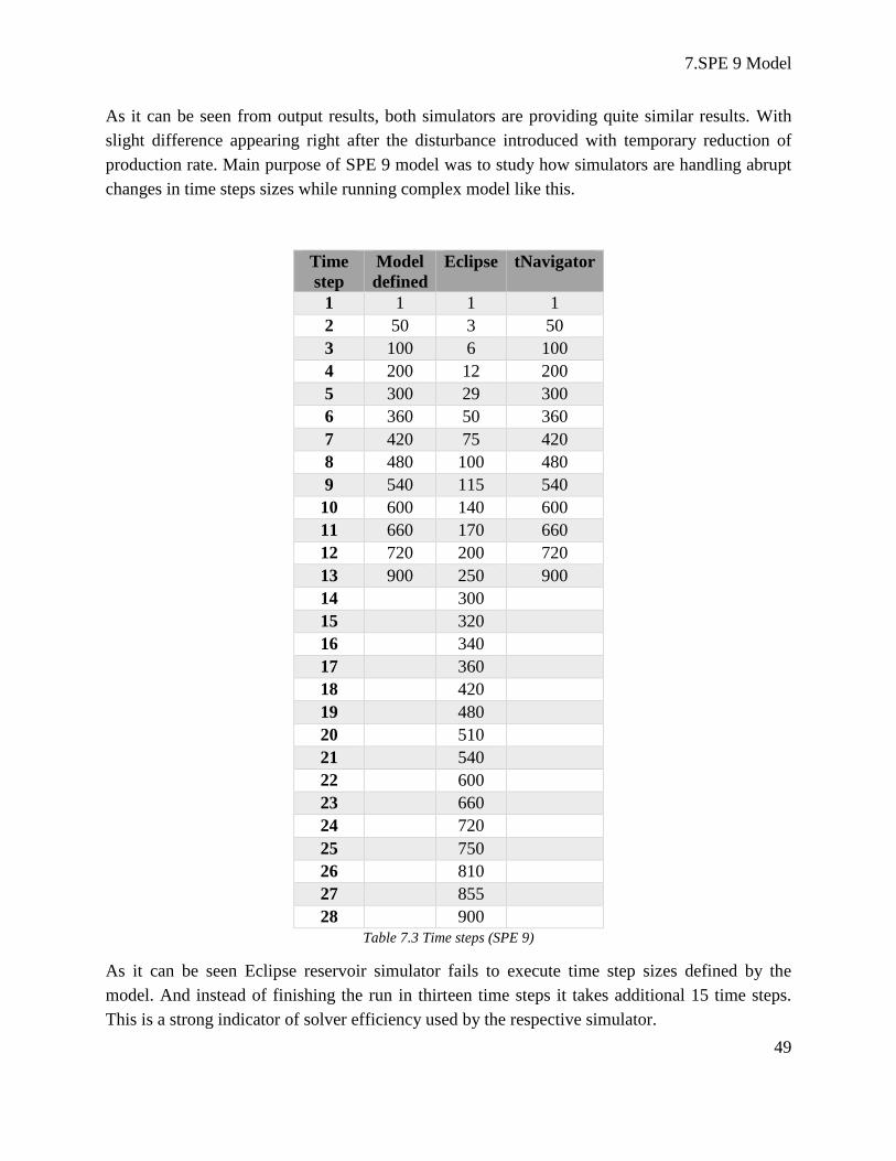
As it can be seen from output results, both simulators are providing quite similar results. With
slight difference appearing right after the disturbance introduced with temporary reduction of
production rate. Main purpose of SPE 9 model was to study how simulators are handling abrupt
changes in time steps sizes while running complex model like this.
Time
step
Model
defined
Eclipse tNavigator
1 1 1 1
2 50 3 50
3 100 6 100
4 200 12 200
5 300 29 300
6 360 50 360
7 420 75 420
8 480 100 480
9 540 115 540
10 600 140 600
11 660 170 660
12 720 200 720
13 900 250 900
14
300
15
320
16
340
17
360
18
420
19
480
20
510
21
540
22
600
23
660
24
720
25
750
26
810
27
855
28
900
Table 7.3 Time steps (SPE 9)
As it can be seen Eclipse reservoir simulator fails to execute time step sizes defined by the
model. And instead of finishing the run in thirteen time steps it takes additional 15 time steps.
This is a strong indicator of solver efficiency used by the respective simulator.

8.Conclusion
50
8. Conclusion
Under this study we have executed all the steps explained in strategy section. From establishing
fair comparison environment by matching results of simple models, to running convergence
study by increasing complexity of models and monitoring respective runtimes. As a final
comparison we had SPE 9 model.
By taking into account all observed results, we could say that both simulators are providing quite
similar output results (variations of max 5% were observed). Regarding runtime of simulations,
we have observed quite similar runtimes for low complexity models, while for more complex
models we start to notice mismatch in runtimes. And if trends of runtimes observed extend in the
same fashion, we can make a conclusion that tNavigator is faster and deals better with models of
higher complexity.
As well in the final study of SPE 9 model runs, we could see that tNavigator manages to deal
with demanding time steps, while Eclipse fails to do so and is forced to break time steps. That
results in higher CPU runtimes. If we take this as an indicator of solver efficiency and capability
to converge even with larger time steps, then we could definitely say that tNavigator simulator is
more efficient.
Regarding the work itself in both of these simulators, my personal impression is that tNavigator
is quite user-friendly compared to Eclipse, and provides very useful feature to monitor your
calculations real time during every time step. It’s strength lays in parallel computing and full
utilization of computer hardware, that practically means that the better computer we use more
efficient it becomes compared to old industry standard software such as Eclipse.

9.Bibliography
51
9. Bibliography
[1] Chen, Z. (2001). Formulations and Numerical Methods of the Black Oil Model in Porous
Media. SIAM Journal on Numerical Analysis, 489-514.
[2] Dake, L. P. (2013). The practice of reservoir engineering.
[3] Ertekin, T. A.-K. (2001). Basic applied reservoir simulation.
[4] Ewing, R. E. (1983). The mathematics of reservoir simulation. Society for Industrial and
Applied Mathematics.
[5] Killough, J. E. (1995, January). Ninth SPE comparative solution project: a reexamination
of black-oil simulation. SPE Reservoir Simulation Symposium.
[6] Pengbo Lu, B. B. (2011). An Adaptive Newton's Method for Reservoir Simulation. SPE
Reservoir Simulation Symposium.
[7] Reservoir Engineering. (2013). Heriot Watt University .
[8] Schlumberger. (2010). ECLIPSE (ECLIPSE* reservoir simulation software Version
2010.1) Reference Manual.


