SYSTEM RELIABILITY ANALYSIS FOR HVDC POWER TRANSMISSION
PAOLA ANDREA GONZALEZ RUEDA
UNIVERSIDAD DE LOS ANDES FACULTY OF ENGINEERING ELECTRIC AND ELECTRONIC
SANTAFE DE BOGOTÁ D.C. 2012

SYSTEM RELIABILITY ANALYSIS FOR HVDC POWER TRANSMISSION
PAOLA ANDREA GONZALEZ RUEDA
THESIS TO OBTAIN THE TITLE OF MASTER IN ENGINEERING AREA: ELECTRICAL ENGINEERING
ASESOR Ing. PHD MARIO ALBERTO RÍOS MESIAS
UNIVERSIDAD DE LOS ANDES
FACULTY OF ENGINEERING ELECTRIC AND ELECTRONIC SANTAFE DE BOGOTÁ D.C.
2012

1
TABLE OF CONTENTS
Figure List ............................................................................................................... 3
Table List................................................................................................................. 4
I. INTRODUCTION ................................................................................................. 4
II. OBJECTIVES...................................................................................................... 5
2.1. General Objective....................................................................................... 5
2.2. Specific Objectives ................................................................................... 5
III. PROBLEM DEFINTION ..................................................................................... 6
IV. THEORETICAL FRAMEWORK ........................................................................ 7
4.1. High Voltage Direct Current Transmission (HVDC) .................................. 7
4.1.1 Classification of HVDC ..................................................................... 10
4.1.2 Components of HVDC Transmission Systems ................................. 11
4.2 Systems Reliability ................................................................................... 11
4.2.1 Reliability in reparable systems ........................................................ 12
4.2.2 Group Reliability of reparable systems ............................................. 12
4.2.3 Monte Carlo Simulation .................................................................... 13
V. IMPLEMENTED METHODOLOGY.................................................................. 16
5.1 Routine Parameters .................................................................................. 16
5.2 Input Variables .......................................................................................... 16
5.3 Structure of the routine .............................................................................. 17
5.3.1 Calculation of the HVDC reliability parameters ................................ 18
5.3.2 Routine to generate the base case .................................................. 22
5.3.3 Routine to obtain the system reliability index ................................... 24
VI. TEST OF THE SIMULATION ROUTINE ........................................................ 29
6.1 IEEE RTS-96 two areas system ............................................................... 31
6.2 Results of the IEEE RTS 96-1 without HVDC ........................................... 33
6.3 Results of the IEEE RTS 96-1 with HVDC ................................................ 35
VII. CONCLUSIONS ............................................................................................. 39
REFERENCE ........................................................................................................ 40
ANNEX A: Programs for reliability analysis .......................................................... 41

2
FIGURE LIST
Figure 1: Monopole HVDC link ................................................................................ 7
Figure 2: Bipolar HVDC link ..................................................................................... 8
Figure 3: Homopole HVDC link ............................................................................... 8
Figure 4: Structure of the HVDC link ....................................................................... 9
Figure 5: Markov process of two states ................................................................. 11
Figure 6: Configuration in Series ........................................................................... 13
Figure 7: Configuration of two elements in parallel ............................................... 13
Figure 8: Simulation of System’s Contingences .................................................... 14
Figure 9: Main Structure of the program ................................................................ 17
Figure 10: Electric HVDC configuration of the Momopole case ............................ 18
Figure 11: Reliability diagram HVDC system ........................................................ 19
Figure 12: Reliability diagram by groups ............................................................... 20
Figure 13: Reliability diagram of three states ........................................................ 20
Figure 14: Unification to one state ......................................................................... 22
Figure 15: Algorithm of the case base ................................................................... 23
Figure 16: Percentages of load for the study case ................................................ 24
Figure 17: Algorithm to the main routine ................................................................ 25
Figure 18: Schematic for the FAULT of one .......................................................... 26
Figure 19: IEEE RTS-96 two areas systems ......................................................... 32
Figure 20: ENS estimator in during the time .......................................................... 33
Figure 21: ENS to Area 1 ....................................................................................... 34
Figure 22: ENS to Area 2 ....................................................................................... 34
Figure 23: ENS of the system ................................................................................ 35
Figure 24: Cost of not supply energy ..................................................................... 35
Figure 25: ENS estimator in during the time .......................................................... 35
Figure 26: ENS of Area 1 ....................................................................................... 36
Figure 27: ENS of Area 2 ....................................................................................... 36
Figure 28: ENS of the System ............................................................................... 36
Figure 29: CENS of the system ............................................................................. 36

3
TABLE LIST
Table I: Reliability parameters of elements of the HVDC link .............................. 19
Table II: Reliability parameters of HVDC Link ...................................................... 22
Table III: Cost of not Supply Energy .................................................................... 27
Table IV: Costs Generator units for the system IEE RTS 96 nodes .................... 29
Table V: User Distribution on nodes PQ for the IEEE RTS 96 two areas ........... 31
Table VI: Parameters for HVDC link .................................................................... 32
Table VII: Computation time and size of the structure ......................................... 33
Table VIII: Results of the simulation for the IEEE-System without HVCD link .... 34
Table IX: Results of the simulation for the IEEE-System with HVCD link ........... 37
4
I. INTRODUCTION
HVDC links have being becoming important for the development of large power
system. For example in China the study on HVDC systems is speeded up by the
project of “power transmission from West to East China” and the economic
system integration. The main reason for the use of these types of links are an
economic alternative scheme for long power transmission and a practical solution
when HVAC systems with is not possible. And another reason to implement
HVDC links is a suitable solution for interconnecting HVAC systems with different
frequencies and control policies, particularly between large isolated HVAC
systems.
Others reasons are that they could provide a better reliability in a high voltage
transmission system. Further this lines works with power control allowing make
load shedding by areas in a case that a contingency is presented in any line in
the zone.
The probabilistic technique is used to analyze the reliability in HVAC systems. In
this document I am going to explain the methodology implement that consist in a
probabilistic technique which is going to simulate the system fault modes with
and without HVDC link between areas.
The main propose of this document is study the reliability of a systems with and
without HVDC link. The developed models and computational techniques based
on the Markov model and reliability diagram which recognized the systems
general configuration and simulate the corresponding operational practice and
the characteristic more efficient and realistically.

5
II. OBJECTIVES
2.1 General Objective
Perform reliability analysis for a power system that employs a HVDC line
interconnecting two areas.
2.2 Specific Objectives
• Determine the rate of repair and failure for a HVDC line, from all independent
rates of the elements that form the HVDC system.
• Perform routine using MATLAB programming and platform PSAT, allowing
calculation of reliability indices of a system with and without an HVDC line.
Given the operating characteristics as economic dispatch, chargeability
system, the costs of not providing the service and the impact of failures
(failure rates and repair both).

6
III. PROBLEM DEFINTION
Nowadays in the world is increasing the implementation of the High Voltage
Direct Current lines (HVDC) like a solution for large capacity transmission over
long distances at high voltage between two asynchronous networks, and different
control policies. It has been the need to make reliability analysis to HVDC
systems; taking in account the operating as economic dispatch, system’s
chargeability, the costs of not providing the service and the system contingencies
as DC, AD line failure and generators.
The other problem is finding the reliability parameters for the HVDC link which
has the problem that has many parts with different rates. The dimension is often
large a difficult to make a consist model.

7
IV. THEORETICAL FRAMEWORK
4.1 High Voltage Direct Current Transmission (HVDC)
The High Voltage Direct Current Transmission HVDC back-to-back has been
used since 1950 to transmitted energy over long distance, to connect two
networks where an AC ties would not be feasible because of system stability
problems or a difference nominal frequencies, and underwater cables for high
capacitance of the cables.
The HVDC links have the ability to rapidly control the transmitted power. For that
reason they have a huge impact on AC stability, a proper design of the HVDC
controls is essential to ensure satisfactory performance of the overall ac/dc
systems.
4.1.1 Classification of HVDC
HVDC links can be classified into the following categories:
• Monopole links: The basic configuration of a monopole link is shown in
Figure 1. This use one conductor, it is usually of negative polarity and the
return is provided by ground or water. In the cases where the earth resistivity I
too high or possible interference with the environment is necessary to use a
metallic return. [1]
Figure 1: Monopole HVDC link
• Bipolar link: This link has the configuration shown in Figure 2. It has two
conductors; one positive and the other one negative. Each terminal has two

8
converters of equal rate voltage connected in series on DC side. The
connection between the converters is grounded. As a rule, the currents in the
two poles are equals in the case that there is no connection to earth. The two
poles could operate independently. In the case that one pole is isolated due to
a fault on its cable, the other pole could work with the ground and thus
transport the half the rate load or more by using the overload capabilities of
its converters and line. Additionally if is a lighting the bipolar link is
considered to be equivalent to a double circuit in AC transmission line. [1]
Figure 2: Bipolar HVDC link
• Homopole link: This link has the configuration shown in Figure 3 this one
has two or more conductors, all having the same polarity. Usually a
negative polarity is used because it causes les radio interference do to
corona. The return path for this type of system is through ground. In the
case that an fault occurs in one of the conductors, the entire converter is
available to supply the remaining conductors which, have some overload
capability, can carry the whole power.[1]
Figure 3: Homopole HVDC link

9
4.1.2 Components of HVDC Transmission Systems
The main components associated with an HVDC system is shown in the Figure 4
using a monopole system as an example. The components for the configuration
are essentially the same as those illustrate in the Figure 4.[1]
Figure 4: Structure of the HVDC link
• Converters: They make possible AC/DC and DC/AC conversion, and they
consist of two poles; each contains two bridges in series. The valve bridges
consist of high voltage thyristor connected in a 6-pulse or 12-pulse
arrangement. The transformers connected to the converters provided
ungrounded three-phase voltage source of appropriate level to the valve
bride. With transformer ungrounded, the DC system has the ability to
establish its own reference to the ground, by grounding the positive or
negative end of the valve.[1]
• Smoothing Reactor: These are reactors which have inductances of 1.0 H
connected in series with each pole of each converter station. They are used
to decrease harmonic voltages and currents in the DC line; limit the crest
current in the rectifier during short-circuit on the line; prevent commutation
fault in inverters and current from being discontinuous at light load.[1]
• Harmonic Filters: These helps to filter the harmonics which are generated
by the converters. Because the harmonics may cause overheating of
capacitors and nearby generators, and interference with telecommunications
systems. [1]

10
• Reactive Power Supplies: Under steady-state conditions, the reactive
power consumed by the line is about 50% of active power transferred. Under
transient conditions, the consumption of reactive power may be increased.
For that reason the reactive power supplies are used close to the converter
stations. In the case where the AC systems are strong they are usually used
as in the form of shunt capacitors. [1]
• DC Line: The DC line could be overhead lines or cables. The one difference
with the AC lines is the number of conductors and spacing.[1]
• AC circuits breakers: These are used to clear the faults in the AC side and
to take out the DC link. They are not used to clear faults on the DC side
because is more effectible the converter control.[1]
4.2 SYSTEMS RELIABILITY
The reliability is the probability of an element or system has an adequate
performance for a period of time considering the establish conditions of
operation. This means that the system must have the ability to supply the full
users’ demand to static or dynamic conditions.
The reliability in power systems could be resumed by different types of index,
which depend of the system which is going to be analyzed. In our case that is a
generation topology; is going to be used the next type of index:
• Loss of Load Expected Value (LOLE): is the expected time (days, hours)
in a define period of time (years, months) in which the load excess the
available generation.
=
(1)
N: Number of the load’s levels by days intervals
: Duration of the load’s level j
: Magnitude of the load’s level j

11
: Load for the interval of time
• Loss of Load Probability (LOLP): is the probability of the available
generation is not capable of supply de demand in a define period of time.
• Expected Value of Energy no Supply (ENS): Is the expected value of
energy in a year which is not given because of exists or failures of
generators or lines.
• Expected Value of Energy no Supply Cost (CENS): is the cost
associated with the energy no supply, this cost depends of the type of user
which is disconnect or the supply is less.
4.2.1 Reliability in reparable systems
This is a stochastic process which is form by cycles of operation-reparation-
operation that could me modeling by different states and probabilities between
states. This is known as Markov process.
For a Markov systems of two states given by the
Figure 5 in which is taken in account exponential probability distributions to stay in
each state: F(t) to the state operates and G(t) to the state No Operates.
Figure 5: Markov process of two states
The functions are defined by these equations:
= − (2) = − (3)
Operates
No Operates
λ µ
12
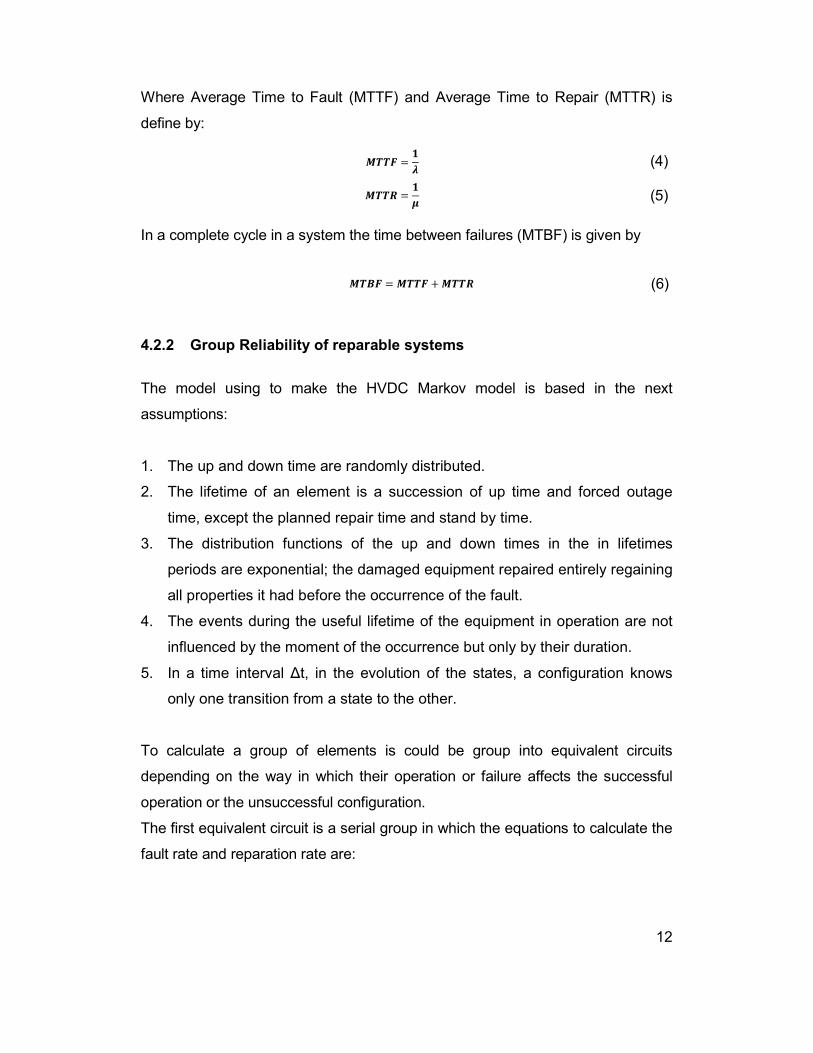
Where Average Time to Fault (MTTF) and Average Time to Repair (MTTR) is
define by:
= (4)
= (5)
In a complete cycle in a system the time between failures (MTBF) is given by
! = + (6)
4.2.2 Group Reliability of reparable systems
The model using to make the HVDC Markov model is based in the next
assumptions:
1. The up and down time are randomly distributed.
2. The lifetime of an element is a succession of up time and forced outage
time, except the planned repair time and stand by time.
3. The distribution functions of the up and down times in the in lifetimes
periods are exponential; the damaged equipment repaired entirely regaining
all properties it had before the occurrence of the fault.
4. The events during the useful lifetime of the equipment in operation are not
influenced by the moment of the occurrence but only by their duration.
5. In a time interval ∆t, in the evolution of the states, a configuration knows
only one transition from a state to the other.
To calculate a group of elements is could be group into equivalent circuits
depending on the way in which their operation or failure affects the successful
operation or the unsuccessful configuration.
The first equivalent circuit is a serial group in which the equations to calculate the
fault rate and reparation rate are:

13
Figure 6: Configuration in Series
=#
# (7)
= $∑ ###
(8)
The second equivalent circuit is two elements in parallels in which the equations
to calculate the fault rate and reparation rate are:
Figure 7: Configuration of two elements in parallel
(9)
= + & (10)
4.2.3 Monte Carlo simulation
This simulation that is used to imitated a time operation of a process or system
which has behavior of Markov model. There are two types of analysis the analytic
or probabilistic.
The analytic method represents the system like a mathematical problem and
calculates the reliability index of any system through the calculated equations.
The probabilistic method consists in a series of random simulations in which
results are the approximation of the reliability index.
The base of this methodology is the generation of random numbers with uniform
distribution between 0 and 1 with the properties of uniformity and independence.
The method used is the inverse transformation. This technique could be
generated an exponential, Weibull or Gumbel distribution the upside is that is
1 2 n
1
2

14
easy to generate a program and the down side is not always computational
efficient.
For a random variable X with a uniform probability distribution FX(x), which is not
decreasing, there is possible to define an inverse function for any number
between 0 and 1.
' = () (11)
In this case is used an exponential function:
*(+ = ,-./0 + 2 0
0+ 4 0 (12)
(+ = 1 − ./0 (13)
Replacing FX(x) for U (random number U (0, 1)) clear X is obtain with exponential
distribution:
' = 6− 1-7) (14)
Where in this case α could be replace with λ that is the fault rate or µ the repair
rate.
Using the equation (14) a departure point you could generate random failures y
reparation times of a system in made by sequential simulation which consists in
created random numbers to each system elements y evaluate the results.
Figure 8: Simulation of System’s Contingences

15
For a define period time t1 to t2 is generate random and independent numbers to
the faults y repairs times for each one of the elements they could have the same
state if is the case for fault state it’s called simultaneous contingencies. From the
end simulation is calculated the reliability index of a contingency during define
period time.
The simulation could be made in to difference ways the first one is determinate
the number of realizations that are necessary to take to an end or calculate a
stop standard to the simulation.
8 = 9:√ (15)
Where:
σ: is the standard deviation of the of the random variable
µ: Correspond media value of the random variable
n: is the number of realizations made
To establish a value of convergence 8 to a system is necessary to run a couple
of simulations and with the result is calculated the values of the coefficient which
allow obtain the closes to the real value in a simulation time.
16
V. IMPLEMENTED METHODOLOGY
The implement methodology consist in two parts the first part is calculated the
fault and repair rate and second part is implement a Monte Carlo simulation
using MATLAB 7.1.0 where in each simulation correspond a year (8760 hours).
Where the system with contingencies are evaluated using the analysis tool of
PSAT. For each scenery is taken the necessary actions by area by changing the
decrease load. With the information of the loss of generation and load; the
program will proceed to calculate the reliability index ENS for each realization and
using the cost of not supply y how is configured the load in each nodes to
calculate the cost of not supply energy (CENS).
Because is necessary to calculate the reliability with not HVDC link the
methodology is the same with the difference of not calculating the HVDC
reliability parameters.
5.1 Routine Parameters
The routine has the next parameters:
• The program is a Monte Carlo sequential simulation which takes in
account the conditions of load and generation for a given hour.
• The program must have a convergence criterion to allow have a result to
the simulation.
• The simulation has for result de reliability index of the system ENS Y
CENS by area and total.
5.2 Input Variables
To elaborate the routine is needed the next information:
• The system information (nodes, generators, lines, transformers, generators’
cost, loads)
• Annual curve of load.

17
• The fault rate (λ) and repair time (µ) for the lines, transformers and
generators.
• The fault rate (λ) and repair time (µ) for each part for the HVDC line to
calculate for the total MTTF and MTTR to the line.
• The maximum apparent power to the lines and transformer y the short time
(15 to 30 minutes).
• The distribution of the type of loads (Industrial I and II, residential or
commercial).
5.3 Structure of the routine
Having the input parameters of the system is defined the three main parts of the
routine; the structure is shown in the Figure 9 which presents the black box of
inputs and exits of the all program.
Figure 9: Main Structure of the program
The total routine is former by one calculation and two main codes, the calculation
is to obtain the total fault and reparation rate to HVDC link from the individuals’
parameters of the elements of the stations of the High Voltage Direct. The first
routine is for modify the generation to supply the load change for each hour of the
year. The second routine how is shown in the Figure 9 is the Monte Carlo routine
which is used calculated the reliability index.

18
5.3.1 Calculation of the HVDC reliability parameters
The technique to determinate the reliability of the HVDC station is created
Markov model of three states based in to the electrical model in the Figure 10.
The block diagram recognizes the system as a general configuration and
simulates the corresponding operational practice.
Figure 10: Electric HVDC configuration of the Momopole case
The block diagram reflects the relations between the subsystems are
constructed. The reliability diagram is constructed using the following rules:
1. The subsystems must be arranged in series when one fault causes when
one fault causes others to be unusable.
2. Subsystems must be arranged in parallel when their fault has no effect on
the availability of others.
3. The overall capacity of subsystems in series in the minimum capacity of
the subsystem.
4. The overall capacity of subsystems in parallel is the sum total capacity of
the subsystems.
The total reliability diagram of the HVDC link is given by the individual reliability
(Figure 11 and Table I).[6]

19
Figure 11: Reliability diagram HVDC system
Table I: Reliability parameters of elements of the HVDC link
COMPONET FALIURE RATE REPARTION RATE
AC Filter 0.775 6
Capacitor 0.002 12
Transformer (3ϕ) 0.023 1140
DC cable 0.0032 792
Valves Group 0.302 6.2
Aux. Power Supply 1 8
Breaker 0.163 94.4
Smoot reactor 0.03 2400
DC Filter 0.775 6
With the rules given previously and the diagram present in the Figure 11, is used
the equations to make groups of the series elements and the parallel elements:
The equations to the series elements are:
<= =<>?
> (16)
:= = <=∑ <>:>?>
(17)
The equations to the parallel elements are:
<= = <<@: + :@::@ + <:@ + <@: (18)
:= = : + :@ (19)
The reliability diagram is defined the following way:

20
Figure 12: Reliability diagram by groups
Where the groups are defined in this form:
1) The AC Group 1 and 2: Are the AC filter parallel whit the Capacitor
2) The Bridget Subsystems 1, 2, 3 and 4: Are the circuit breaker, the
transformer, the rectifier or the investor in series configuration
3) Line Subsystem: Is the Auxiliary supply, reactors, DC Filters, DC link.
One the main advantages which have an HVDC link is the ability to transfer the
half of the power. In the monopole case is present that line works in 50 % of the
capacity when a contingence is one of the elements of the Valve Subsystems but
only in only group. If the case that two elements of different Valves Subsystems
the HVDC module will not be able to work.
Figure 13: Reliability diagram of three states
To reduce the block diagram of the Figure 12 to the three states I analyzed the
possible combinations to be able to find a patron. The possible combinations are:

21
1. Working in 100%: AC Groups 1 and 2, the Valves Groups 1 to 4 and DC
Line group are working.
2. Working in 50%: There are four options could be defined
a. AC Subsystems 1 and 2, DC Line Subsystem, the valve subsystems 2,
3, and 4 are working and the valve subsystem 1 not working.
b. AC Subsystems 1 and 2, DC Line Subsystem, the valve subsystems 1,
3, and 4 are working and the valve subsystem 2 not working.
c. AC Subsystems 1 and 2, DC Line Subsystem, the valve subsystems 1,
2, and 4 are working and the valve subsystem 3 not working.
d. AC Subsystems 1 and 2, DC Line Subsystem, the valve subsystems 1,
2, and 3 are working and the valve subsystem 4 not working.
3. Working in 100%: This state is arrived when one of these combinations of
elements is not working.
a. AC Subsystems 1 or 2 not working.
b. DC Line Subsystems not working.
c. The valve Subsystems 1 and 2 not working
d. The valve Subsystems 3 and 4 not working
With the information given be in one state is possible to combined the states
because the rate change of those states goes to the same states. For that reason
the states 2a, 2b, 2c, 2d could be unified in only one state. With se sum of the all
fault rates to go 50% HVDC working and to go back to the state 100% working
from 50% work state is only required used one reparation rate because is equal
for all the valve group.
The same case happens when the systems goes from the state of 50% working
to the state of the HVDC doesn’t works. Whit the different of that the fault rate to
go to 0% is equal to the sum of the 3 rest fault rates of the valves subsystems
and is the same that the case before to defined reparation rate.

22
Figure 14: Unification to one state
To define the fault and repair rate to go from the state 100% works to 0% works I
calculated the parallel between the valve subsystems 1 and 2 and the same to
the valve subsystems 3 and 4.Then all the subsystems in series having the next
results:
Table II: Reliability parameters of HVDC Link
STATE FAULT RATE REPARATION RATE
100% Working 6.0364 (λ1) 26.00 (µ3)
50% Working 0.0747 (λ2) 54.97 (µ2)
Not working 0.0007 (λ3) 1.0243 (µ1)
5.3.2 Routine to generate the base case
The routine to generate the base case is shown in the Figure 15. This routine has
incited the annual percentage of load to hour having in account the season of the
year and the systems sin which is going to be calculated.
Valve Sub 1
Valve Sub 2
Valve Sub 3
Valve Sub 4
50% HVDC
WORKING
<AB
A

23
Figure 15: Algorithm of the case base
The routine began with the preload of the annual load percentages to the case
system Figure 16. The next step is calculate the new load by multiplied the
percentage of load to the nodes type PQ, next sum the values of active power of
the nodes PQ to obtain the maximum value of load. From each value of
maximum load for each hour is made the order merit dispatch using a quadratic
function cost to determinate the costs of Turing on the generators connected at
the nodes PV. Then is organized the costs by the minor to mayor value so it can
be dispatch to the maximum value until is reach the maximum value of load for
each hour.

24
Figure 16: Percentages of load for the study case
With the dispatch vector for each hour the system is modified with the respective
changes in the load, Supply and nodes PQ. Then is make the power flow and the
voltages results are evaluate to verified there are not violations in all nodes and
that the generators works in the power limits. For the reason that is used to make
the dispatch the merit order and sometimes is not enough the generators on to
supply the load for each hour so the next generator in the list or merit order is
dispatch and the system is evaluated this process is made until there are not any
violations. The dispatch is saved in a matrix for each hour.
5.3.3 Routine to obtain the system reliability index
The routine to calculate the system reliability index is shown in Figure 17. This
routine has preload the merit order dispatch, the fault and repair rates for the
lines, generators and HVDC Link, and the load distributions in the nodes PQ.

25
Figure 17: Algorithm to the main routine
The routine begins to preload the order of merit dispatch, the fault and repair
rates for generators, lines, transformers and HVDC link, the distribution of the
loads in the nodes PQ.
The first step is generating random numbers between 0 to 1 types normal. Using
equation (14) is calculated the failure time. If one of these times is less than 8760

26
is determinate the elements which fails and it is generates the corresponding
value for the time reparation using the same equation (14).
When is determinate every contingencies for the year, they are organized in
falling order according with the failure time and the repair time. This order helps
to find hours which multiples contingencies.
Once it has the vector of the failures times for the realization is made “for” cycle
where is pass every hour of the vector. The cycle consist in the calculate the
base case for each failure hour and the power flow taking in account the
contingencies so it can be obtain the system state. In the results of the power
flow is made four types of evaluations:
1. It’s evaluated the convergence of the power flow. If is the case that the
system does not converge the counter of not convergence is
incremented and the ENS is calculated by the sum of the all the active
power of the nodes PQ.
2. It’s evaluated if any of the connection between areas links is not working
if is the case is apply the automatic shedding. In the Area 1 the
generation and the area 2 loads depending on how much is different
between the load and the generation.
Figure 18: Schematic for the FAULT of one Or more interconnection area link
3. It’s evaluated if there are loss of generation of the system having in
account the available generators, the conditions on the nodes PV and
Slack. If the power in the PV node is less than the generation available,
so is reduced the power in the proportional form. The shedding is made
AC link
HVDC link Area 1 Area 2
Loss Generation
AC link
Loss of load
27
in the nodes slack and in the nodes closed to the slack node and in the
area where is present the contingence.
4. It’s evaluated if there are overload in the lines, if one or more lines
presents overloads, is apply and operator action that could be in 10 to
100 MW in one in the nodes closed to the overload line.
From the evaluations of overload, Inter-area links fault and the loss of
generators is obtain the magnitude of power reduced by node in the systems
and sum of all them is the amount of energy not supply by area and total.
When is evaluated every failure hours in the realization is obtain the vector
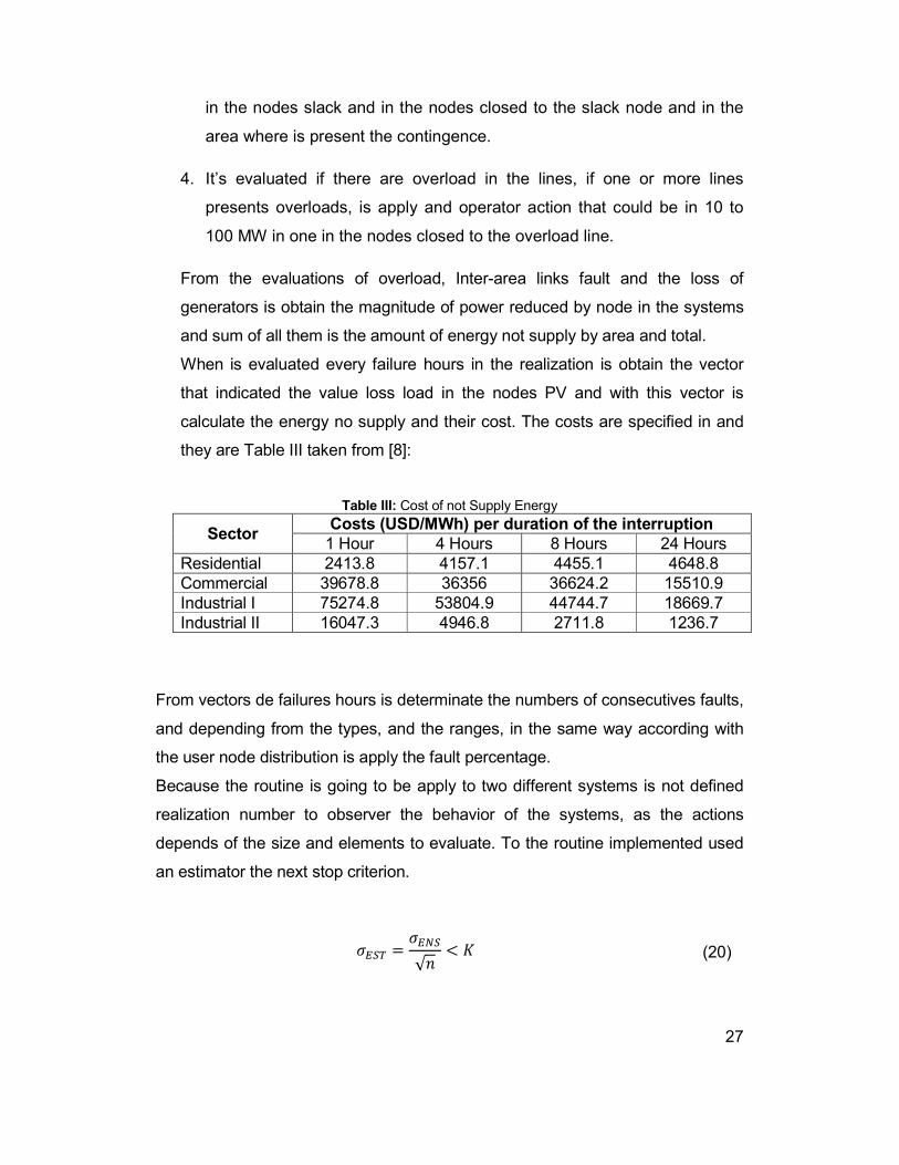
that indicated the value loss load in the nodes PV and with this vector is
calculate the energy no supply and their cost. The costs are specified in and
they are Table III taken from [8]:
Table III: Cost of not Supply Energy
Sector Costs (USD/MWh) per duration of the interruption
1 Hour 4 Hours 8 Hours 24 Hours
Residential 2413.8 4157.1 4455.1 4648.8
Commercial 39678.8 36356 36624.2 15510.9
Industrial I 75274.8 53804.9 44744.7 18669.7
Industrial II 16047.3 4946.8 2711.8 1236.7
From vectors de failures hours is determinate the numbers of consecutives faults,
and depending from the types, and the ranges, in the same way according with
the user node distribution is apply the fault percentage.
Because the routine is going to be apply to two different systems is not defined
realization number to observer the behavior of the systems, as the actions
depends of the size and elements to evaluate. To the routine implemented used
an estimator the next stop criterion.
9CDE = 9CD√ 4 F (20)

28
The estimator is standard deviation from the data of the ENS’s vectors divided
the square root of the number on the realizations. For to the simulation’s cycle
the value must be less to the 2.5 MWh.

29
VI. TEST OF THE SIMULATION ROUTINE
The routine was written for the system IEEE RTS of two areas (48 nodes). The
simulations were made in computer processing unit INTEL i5. The operative
system is Windows 7; the MATLAB and PSAT version was 7.1 and 4.2.1.
The connection data and the fault and repair rates from transformers, lines and
generators were taken from [] and edited in the archive .m so it can be modified.
In the same way in the article was given the relative percentages of the load
curve daily, weekly and hourly for every season of the year.
The costs of the generation unit are from the PSAT example of RTS 24 nodes.
These costs by generator are defined in the system use a quadratic cost function.
GH = IJ@H@ + IJH + IJK (21)
In the Table IV is present de values of a, b and c for each generator unit for the
48 nodes.
Table IV: Costs Generator units for the system IEE RTS 96 nodes
Node Generator
Unit
Type Generator
Unit
Pmax [MW]
L$ [US/H]
L [US/MWh]
L& [US/MW.MWh]
1
U20 Oil/CT 20 1,72 24,8415 0,36505
U20 Oil/CT 20 1,72 24,8415 0,36505
U76 Coal/Steam 76 3,5 10,2386 0,038406
U76 Coal/Steam 76 3,5 10,2386 0,038406
2
U20 Oil/CT 20 1,72 24,8415 0,36505
U20 Oil/CT 20 1,72 24,8415 0,36505
U76 Coal/Steam 76 3,5 10,2386 0,038406
U76 Coal/Steam 76 3,5 10,2386 0,038406
7
U100 Oil/Steam 100 17,9744 0,027485 0
U100 Oil/Steam 100 17,9744 0,027485 0
U100 Oil/Steam 100 17,9744 0,027485 0
13 U197 Oil/Steam 197 0,58 18,47 0,010111
U197 Oil/Steam 197 0,58 18,47 0,010111

30
U197 Oil/Steam 197 0,58 18,47 0,010111
15
U12 Oil/Steam 12 1,09 9,5369 0,005588
U12 Oil/Steam 12 1,09 9,5369 0,005588
U12 Oil/Steam 12 1,09 9,5369 0,005588
U12 Oil/Steam 12 1,09 9,5369 0,005588
U12 Oil/Steam 12 1,09 9,5369 0,005588
U155 Coal/Steam 155 1,11 21,2267 0,379374
16 U155 Coal/Steam 155 1,11 21,2267 0,379374
18 U400 Nuclear 400 5,76 5,2301 6,70E-07
21 U400 Nuclear 400 5,76 5,2301 6,70E-07
22
U50 Hydro 50 0,000067 52.301 5,67
U50 Hydro 50 0,000067 52.301 5,67
U50 Hydro 50 0,000067 52.301 5,67
U50 Hydro 50 0,000067 52.301 5,67
U50 Hydro 50 0,000067 52.301 5,67
U50 Hydro 50 0,000067 52.301 5,67
23
U155 Coal/Steam 155 1,11 21,2267 0,379374
U155 Coal/Steam 155 1,11 21,2267 0,379374
U350 Coal/Steam 350 1,64 9,5856 0,003154
25
U20 Oil/CT 20 1,72 24,8415 0,36505
U20 Oil/CT 20 1,72 24,8415 0,36505
U76 Coal/Steam 76 3,5 10,2386 0,038406
U76 Coal/Steam 76 3,5 10,2386 0,038406
26
U20 Oil/CT 20 1,72 24,8415 0,36505
U20 Oil/CT 20 1,72 24,8415 0,36505
U76 Coal/Steam 76 3,5 10,2386 0,038406
U76 Coal/Steam 76 3,5 10,2386 0,038406
31
U100 Oil/Steam 100 17,9744 0,027485 0
U100 Oil/Steam 100 17,9744 0,027485 0
U100 Oil/Steam 100 17,9744 0,027485 0
37
U197 Oil/Steam 197 0,58 18,47 0,010111
U197 Oil/Steam 197 0,58 18,47 0,010111
U197 Oil/Steam 197 0,58 18,47 0,010111
39
U12 Oil/Steam 12 1,09 9,5369 0,005588
U12 Oil/Steam 12 1,09 9,5369 0,005588
U12 Oil/Steam 12 1,09 9,5369 0,005588
U12 Oil/Steam 12 1,09 9,5369 0,005588
U12 Oil/Steam 12 1,09 9,5369 0,005588
U155 Coal/Steam 155 1,11 21,2267 0,379374
40 U155 Coal/Steam 155 1,11 21,2267 0,379374
42 U400 Nuclear 400 5,76 5,2301 6,70E-07
45 U400 Nuclear 400 5,76 5,2301 6,70E-07
46 U50 Hydro 50 0,000067 52.301 5,67
31
U50 Hydro 50 0,000067 52.301 5,67
U50 Hydro 50 0,000067 52.301 5,67
U50 Hydro 50 0,000067 52.301 5,67
U50 Hydro 50 0,000067 52.301 5,67
U50 Hydro 50 0,000067 52.301 5,67
47
U155 Coal/Steam 155 1,11 21,2267 0,379374
U155 Coal/Steam 155 1,11 21,2267 0,379374
U350 Coal/Steam 350 1,64 9,5856 0,003154
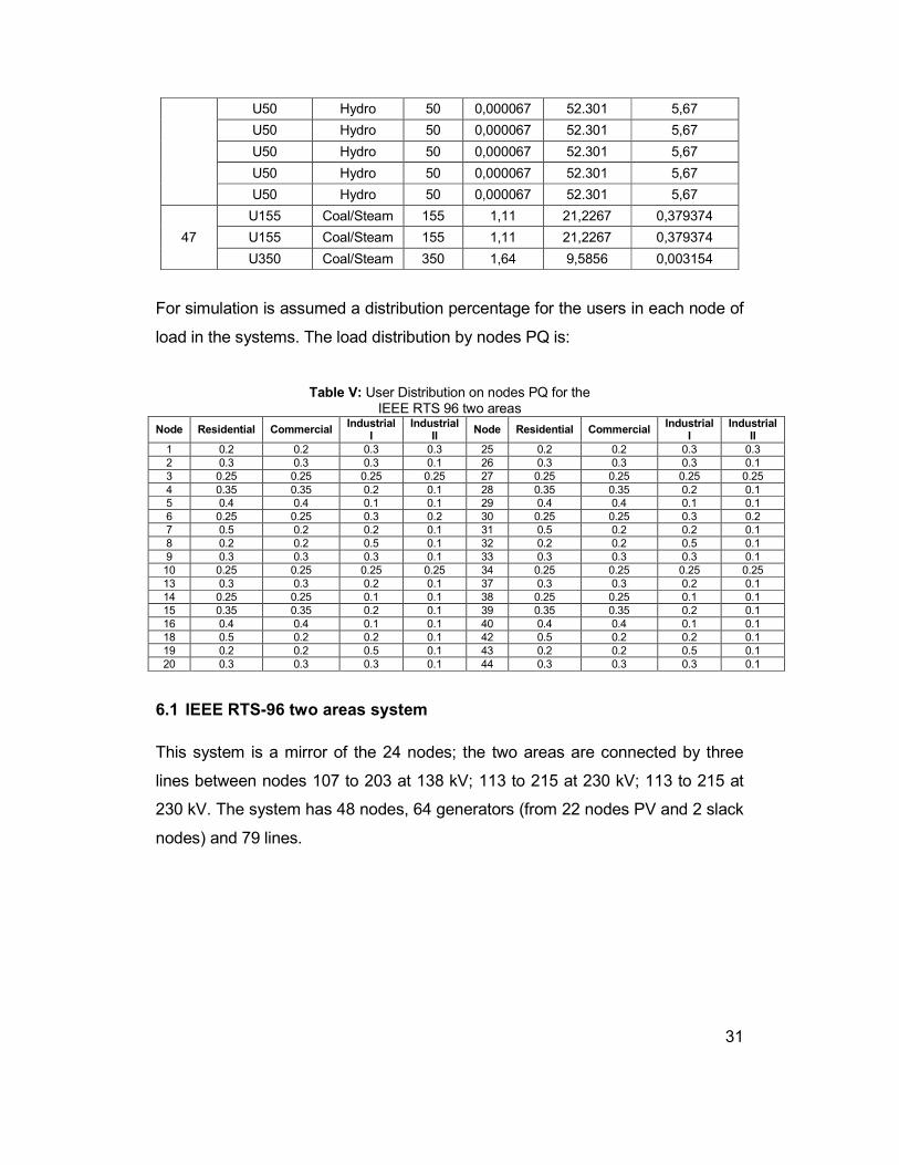
For simulation is assumed a distribution percentage for the users in each node of
load in the systems. The load distribution by nodes PQ is:
Table V: User Distribution on nodes PQ for the IEEE RTS 96 two areas
Node Residential Commercial Industrial
I Industrial
II Node Residential Commercial
Industrial I
Industrial II
1 0.2 0.2 0.3 0.3 25 0.2 0.2 0.3 0.3
2 0.3 0.3 0.3 0.1 26 0.3 0.3 0.3 0.1
3 0.25 0.25 0.25 0.25 27 0.25 0.25 0.25 0.25
4 0.35 0.35 0.2 0.1 28 0.35 0.35 0.2 0.1
5 0.4 0.4 0.1 0.1 29 0.4 0.4 0.1 0.1
6 0.25 0.25 0.3 0.2 30 0.25 0.25 0.3 0.2
7 0.5 0.2 0.2 0.1 31 0.5 0.2 0.2 0.1
8 0.2 0.2 0.5 0.1 32 0.2 0.2 0.5 0.1
9 0.3 0.3 0.3 0.1 33 0.3 0.3 0.3 0.1
10 0.25 0.25 0.25 0.25 34 0.25 0.25 0.25 0.25
13 0.3 0.3 0.2 0.1 37 0.3 0.3 0.2 0.1
14 0.25 0.25 0.1 0.1 38 0.25 0.25 0.1 0.1
15 0.35 0.35 0.2 0.1 39 0.35 0.35 0.2 0.1
16 0.4 0.4 0.1 0.1 40 0.4 0.4 0.1 0.1
18 0.5 0.2 0.2 0.1 42 0.5 0.2 0.2 0.1
19 0.2 0.2 0.5 0.1 43 0.2 0.2 0.5 0.1
20 0.3 0.3 0.3 0.1 44 0.3 0.3 0.3 0.1
6.1 IEEE RTS-96 two areas system
This system is a mirror of the 24 nodes; the two areas are connected by three
lines between nodes 107 to 203 at 138 kV; 113 to 215 at 230 kV; 113 to 215 at
230 kV. The system has 48 nodes, 64 generators (from 22 nodes PV and 2 slack
nodes) and 79 lines.

32
Figure 19: IEEE RTS-96 two areas systems
For the simulation of HVDC is used the next parameters for the link which is
connected from nodes 113 to 205, the line used has a longitude of 1200km
connecting Canada Windors Quebec to United States Franklin New Hampshire:
[7]
Table VI: Parameters for HVDC link
Parameter Value
Control mode Power
DC line resistance (Ω) 5
Power Demand (MW) 100
Scheduled DC Voltage (kV) 500
Compounding resistance (Ω) 5
Margin in per unit desired DC power 0.1
Number of bridges in series 4
Nominal maximum firing angle 15
Minimum steady state firing angle 16
Commutating transformer resistance/bridge Rectifier (Ω) 0.0180
Commutating transformer resistance/bridge Inverter (Ω) 0.0103
Primary base AC voltage (kV) 230
Transformer ratio 0.46
Tap setting Rectifier 1.15452
Tap setting Inverter 0.97987

33
The simulations of the next have next times and size:
Table VII: Computation time and size of the structure
IEEE RTS 96-1 IEE RTS96-1 HVDC
computation time [Hours] 27.9 34.45
size of the structure [MB] 20.3 22.0
6.2 Results of the IEEE RTS 96-1 without HVDC
To IEEE RTS 96-1 without HVDC link it was made two tests the first test the
first was to determined convergence values, for this was made 2000 iterations
to ensure the minimum value of convergence.
Figure 20: ENS estimator in during the time
I could be observed that the estimator began to converge around to 1000 Min
and the value is 3.343 MW-H with a sensibility of 0.798 MW-H. Also it could be
observed that for this case the system has high number at the first past of the
simulation then it has a fast fall down. This system presents 116 contingencies
and 9 no convergences. The results by area for ENS are:

34
Figure 21: ENS to Area 1 Figure 22: ENS to Area 2
It is observer that the maximum values in the simulations are they are not
convergence in the system and it has to retire the entire load also it is observer
that sometimes is shedding load in only one area or both areas. The resume
table where the results are:
Table VIII: Results of the simulation for the IEEE-System without HVCD link
Index AREA1 AREA 2 system
Expected value ENS [MW-h/year] 7,643 5,350 22,929
Standard deviation ENS [MW-h/year]
0,235206 0,09761 0,137629
Expected value CENS [Mill USD/year]
9,70999985
Standard deviation CENS [Mill USD/year]
3,44871142
Epoch of the routine 2000
Compute time of the routine [H] 24
Expected value by epoch [min] 1.234
Percentage of not convergence 0.01246
LOLE 5.251
The energy no supply (ENS) and the Cost of no Supply Energy are:
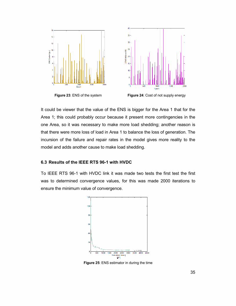
35
Figure 23: ENS of the system Figure 24: Cost of not supply energy
It could be viewer that the value of the ENS is bigger for the Area 1 that for the
Area 1; this could probably occur because it present more contingencies in the
one Area, so it was necessary to make more load shedding; another reason is
that there were more loss of load in Area 1 to balance the loss of generation. The
incursion of the failure and repair rates in the model gives more reality to the
model and adds another cause to make load shedding.
6.3 Results of the IEEE RTS 96-1 with HVDC
To IEEE RTS 96-1 with HVDC link it was made two tests the first test the first
was to determined convergence values, for this was made 2000 iterations to
ensure the minimum value of convergence.
Figure 25: ENS estimator in during the time

36
I could be observed that the estimator began to converge around to 100 Min and
the value is 3.343 MW-H with a sensibility of 0.798 MW-H. This system presents
116 contingencies and 9 no convergences. The results by area for ENS are:
Figure 26: ENS of Area 1 Figure 27: ENS of Area 2
It is observer that the maximum values in the simulations are they are not
convergence in the system and it has to retire the entire load also it is observer
that sometimes is shedding load in only one area or both areas. Next is present
the total Energy not supply in the system with the cost.
Figure 28: ENS of the System Figure 29: CENS of the system
Is observer that the cost of not supply energy is less than the case without
HVDC. The reason is that the areas are less that the areas behave lite two
independent systems, so the load shedding is less and they can operate. For the
case where the HVDC link failure the systems would loss generation in the Area
1 and load in the Area 2, because the other two lines which interconnect the
areas cannot support the power that demand the area 2. The results are:
37
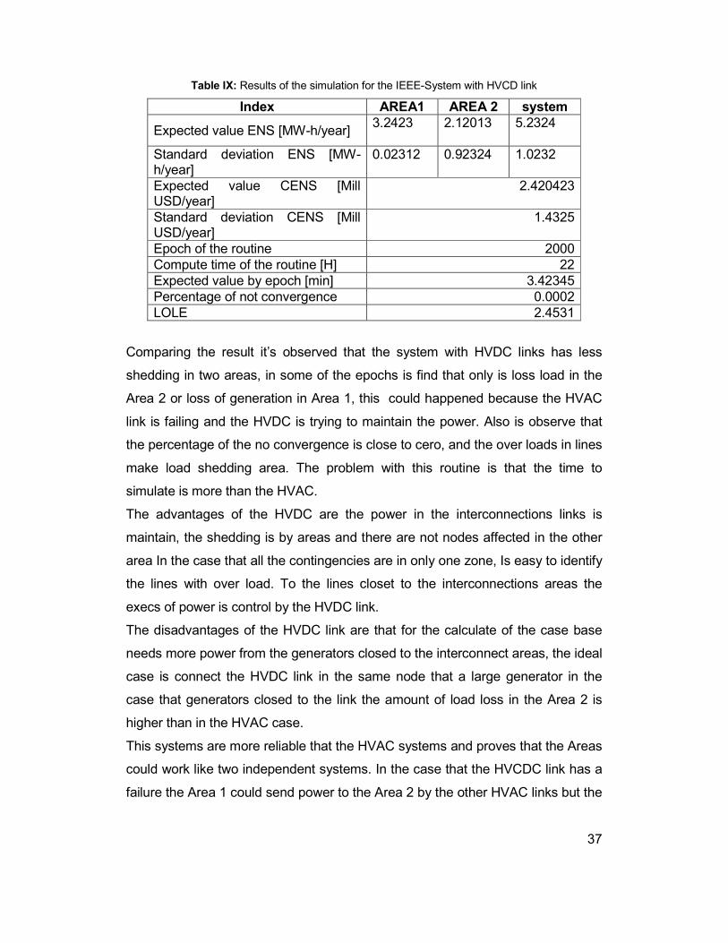
Table IX: Results of the simulation for the IEEE-System with HVCD link
Index AREA1 AREA 2 system
Expected value ENS [MW-h/year] 3.2423
2.12013 5.2324
Standard deviation ENS [MW-h/year]
0.02312 0.92324 1.0232
Expected value CENS [Mill USD/year]
2.420423
Standard deviation CENS [Mill USD/year]
1.4325
Epoch of the routine 2000
Compute time of the routine [H] 22
Expected value by epoch [min] 3.42345
Percentage of not convergence 0.0002
LOLE 2.4531
Comparing the result it’s observed that the system with HVDC links has less
shedding in two areas, in some of the epochs is find that only is loss load in the
Area 2 or loss of generation in Area 1, this could happened because the HVAC
link is failing and the HVDC is trying to maintain the power. Also is observe that
the percentage of the no convergence is close to cero, and the over loads in lines
make load shedding area. The problem with this routine is that the time to
simulate is more than the HVAC.
The advantages of the HVDC are the power in the interconnections links is
maintain, the shedding is by areas and there are not nodes affected in the other
area In the case that all the contingencies are in only one zone, Is easy to identify
the lines with over load. To the lines closet to the interconnections areas the
execs of power is control by the HVDC link.
The disadvantages of the HVDC link are that for the calculate of the case base
needs more power from the generators closed to the interconnect areas, the ideal
case is connect the HVDC link in the same node that a large generator in the
case that generators closed to the link the amount of load loss in the Area 2 is
higher than in the HVAC case.
This systems are more reliable that the HVAC systems and proves that the Areas
could work like two independent systems. In the case that the HVCDC link has a
failure the Area 1 could send power to the Area 2 by the other HVAC links but the

38
cost is higher. In the case that the HVAC links fails the HVDC could provide the
complete amount of power to the other Area.

39
VII. CONCLUSIONS
1. The sequential Monte Carlo simulation is a dynamic way to observe the
behavior of the system to understand what’s happened when is present a
fault in any element of the systems.
2. The methodology of load shedding implemented gives a good vision of
the reality of the power systems with HVDC links, and permits to deduce
that the HVDC link could make two systems work in an independent
form.
3. The problem to the put all the elements of the HVDC link in one block is
resolved using the Markov model. Because it gives a good approach of
the real function of HVDC link.

40
REFERENCES
[1] P. Kundur “Power Systems Stability and Control”, McGraw Hill 1993. [2] Q. Guo, J. Zhao “Faults Predictions and Analysis on Reliability of the ±660kV
Ningdong HVDC Power Transmission System”, Electric Utility Deregulation and Restructuring and Power Technologies (DRPT), 2011 4th International Conference, IPEC 2005, Vol 2, pp 734-739, 2005.
[3] C. Weihua, J. Quanyuan, C. Yijia; Risk based vulnerability assessment for HVDC transmission system; Power Engineering Conference, Vol. 2, pp 734 – 739, 2005.
[4] Aik, D.L.H.; Andersson, G.; “Power stability analysis of multi-infeed HVDC systems”; IEEE Transactions on Power Delivery; Vol 13; pp 923 – 931, 1998.
[5] Basu, K. P; Stability enhancement of power system by controlling HVDC power flow through the same AC transmission line; IEEE Symposium on Industrial Electronics & Applications, 2009. ISIEA 2009. Vol 2; Pag 663 – 668, 2009
[6] E.N. Dialynas, N.G. Koskolos; Reliability modeling and evaluation of HVDC power transmission systems; IEEE Transactions on Power Delivery, Vol. 9, pp 872-870, 1994.
[7] The IEEE Reliability Test System 1996: Application of Probability Methods Subcommittee A report prepared by the Reliability Test System Task Force of the; IEEE Transactions on Power Systems, Vol. 14, NO. 3, August 1999 pp 1010-1020
[8] CERON D AGUILAR G, BOHORQUEZ G. Examen Final Analisis Sistemas de Potencia, Universidad de los Andes
[9] R Billinton and D.S. Ahluwalia, "Incorporation of a DC Link in a Composite System Adequacy Assessment - Composite System Analysis', IEE Roc. C, Vol. 139, No. 3, May 1992.
[10] R Billinton, P.K. Vohra and Sudhir Kumar, 'Effect of Station Originated Outages in a Composite System Adequacy Evaluation of the IEEE Reliability Test System', IEEE PAS, Vol-104, No. 10, Oct. 1985, pp 2644-2656.
[11] B. Poretta, D.L Kiguel, G.A. Hamoud and E.G. Neudorf, 'A Comprehensive Approach for Adequacyand Security Evaluation of Bulk Power Systems", EEETrans. on Power Systems, PWRS, May 1991, pp 433-441.

41
Annex A: Programs for HVAC reliability analysis
BASEAC: Routine which calculates the matrices of the PV, PQ, Supply, SW to
each hour of the year (8760) have has enter the economical dispatch the percent
curve load and the base case.
%Clear all the values clc clear all; Tiempo_0=cputime; %Begin PSAT closepsat; initpsat; clpsat.readfile = 0; clpsat.mesg=0; %Clear the messages of the PSAT %Turn off the warnings warning off MATLAB:divideByZero; warning off MATLAB:nearlySingularMatrixUMFPACK; warning off MATLAB:dispatcher:InexactCaseMatch; Settings.freq=60; [PCYR]=CYR'; %Load the load curve pcarga=CYR'; eval('Info_Gen1'); %Load the generation information runpsat('d_048AC1.m','data') %Load the initial case runpsat ('pf') %run PSAT DAEbase=DAE; Snapshotbase=Snapshot; L_act_in=PQ.con(:,4); %Define the intial Active Power L_react_in=PQ.con(:,5); %Define the intial Reactive Power %Define the temporal variables. PV1=PV.con; Bus1=Bus.con; PQ1=PQ.con; SW1=SW.con; HVDC1=Hvdc.con; Line1=Line.con; Shunt1=Shunt.con; for i=1:8760 pgargah=PCYR(i); PQ1(:,4)=PCYR(i)*L_act_in; PQ1(:,5)=PCYR(i)*L_react_in;

42
%Calculate the Merir order dispatch [TMVDES]=Despacho2(Supply1,PQ1,pgargah); %Calculates the disponible Dispatch and the values of active power the %nodes PV [Supplyt, Gen1, GenSW1, Despacho_Disponible]=source(TMVDES, ... Supply1, Gen, UGEN, UGenSW, GenSW); Supply1=Supplyt; Gen=Gen1; GenSW=GenSW1; GF=find(TMVDES(:,2)==0); %Gives the values of Active Power in the nodes PV SW [PV2,SW2]=NODOSPV1(PV1,SW1,Gen1,GenSW1); PV.store(:,4)=PV2(:,4); PQ.store(:,[4 5])=PQ1(:,[4 5]); SW.store(:,10)=SW2(:,10); %Save the values of in .m archive Guardar2AC(Bus1,Line1,Shunt1,SW.con,PV.con,PQ.con); %Run Past runpsat('CASO48_AC','pf'); PV3=PV.con; %Calculate the Voltages in the node V_temp=DAE.y(1+Bus.n:2*Bus.n); %Verifed the voltage limites [FLAG_V]=v_cond(V_temp); BC=0; IPV(:,i)=PV.con(:,4); IPQA(:,i)=PQ.con(:,4); IPQR(:,i)=PQ.con(:,5); ISW(:,i)=SW.con(:,10); if FLAG_V==1 BC=BC+1; while BC>0 TMVDES(GF(BC),2)=Supply(GF(BC),4); [Supplyt,Gen1,GenSW1,Despacho_Disponible]=source(TMVDES,... Supply1, Gen, UGEN, UGenSW, GenSW); Supply1=Supplyt; %Gives the values of Active Power in the nodes PV SW [PV2,SW2]=NODOSPV1(PV1,SW1,Gen1,GenSW1); PV.store(:,4)=PV2(:,4); PQ.store(:,[4 5])=PQ1(:,[4 5]); SW.store(:,10)=SW2(:,10); %Save the values of in .m archive Guardar2AC(Bus1,Line1,Shunt1,SW.con,PV.con,PQ.con); %Run Past runpsat('CASO48_AC','pf');

43
%Calculate the Voltages in the node V_temp=DAE.y(1+Bus.n:2*Bus.n); %Verifed the voltage limites [FLAG_V]=v_cond(V_temp); if FLAG_V==1 BC=BC+1; elseif FLAG_V==0 BC=0; IPV(:,i)=PV.con(:,4); IPQA(:,i)=PQ.con(:,4); IPQR(:,i)=PQ.con(:,5); ISW(:,i)=SW.con(:,10); break end end end end %Save the values for those nodes in a matriz for each hour of dats GuardarBaseAC(IPV,IPQA,IPQR,ISW); runpsat('d_048AC1.m','data') runpsat ('pf') closepsat; Tiempo_1=cputime-Tiempo_0;
BASEDC: Routine which calculates the matrices of the PV, PQ, Supply, SW to
each hour of the year (8760) have has enter the economical dispatch the percent
curve load and the base case.
%Clear all the values clc clear all; Tiempo_0=cputime; %Begin PSAT closepsat; initpsat; clpsat.readfile = 0; clpsat.mesg=0; %Clear the messages of the PSAT %Turn off the warnings warning off MATLAB:divideByZero; warning off MATLAB:nearlySingularMatrixUMFPACK; warning off MATLAB:dispatcher:InexactCaseMatch; Settings.freq=60; [PCYR]=CYR'; %Load the load curve pcarga=CYR'; eval('Info_Gen1'); %Load the generation information runpsat('d_048DC1.m','data') %Load the initial case

44
runpsat ('pf') %run PSAT DAEbase=DAE; Snapshotbase=Snapshot; L_act_in=PQ.con(:,4); %Define the intial Active Power L_react_in=PQ.con(:,5); %Define the intial Reactive Power %Define the temporal variables. PV1=PV.con; Bus1=Bus.con; PQ1=PQ.con; SW1=SW.con; HVDC1=Hvdc.con; Line1=Line.con; Shunt1=Shunt.con; pcarga=CYR'; for i=1:8760 pgargah=PCYR(i); PQ1(:,4)=PCYR(i)*L_act_in; PQ1(:,5)=PCYR(i)*L_react_in; [TMVDES]=Despacho2(Supply1,PQ1,pgargah); [Supplyt, Gen1, GenSW1, Despacho_Disponible]=source(TMVDES, Supply1,... Gen, UGEN, UGenSW, GenSW); Supply1=Supplyt; Gen=Gen1; GenSW=GenSW1; GF=find(TMVDES(:,2)==0); [PV2,SW2]=NODOSPV1(PV1,SW1,Gen1,GenSW1); PV.store(:,4)=PV2(:,4); PQ.store(:,[4 5])=PQ1(:,[4 5]); SW.store(:,10)=SW2(:,10); Guardar2DC(Bus1,Line1,Shunt1,SW.con,PV.con,PQ.con,HVDC1); runpsat('CASO48_DC','pf'); PV3=PV.con; V_temp=DAE.y(1+Bus.n:2*Bus.n); [FLAG_V]=v_cond(V_temp); BC=0; IPV(:,i)=PV.con(:,4); IPQA(:,i)=PQ.con(:,4); IPQR(:,i)=PQ.con(:,5); ISW(:,i)=SW.con(:,10);
if FLAG_V==1 BC=BC+1; while BC>0 TMVDES(GF(BC),2)=Supply(GF(BC),4); [Supplyt,Gen1,GenSW1,Despacho_Disponible] =source(TMVDES,... Supply1, Gen, UGEN, UGenSW, GenSW); Supply1=Supplyt;

45
%Gives the values of Active Power in the nodes PV SW [PV2,SW2]=NODOSPV1(PV1,SW1,Gen1,GenSW1); PV.store(:,4)=PV2(:,4); PQ.store(:,[4 5])=PQ1(:,[4 5]); SW.store(:,10)=SW2(:,10); %Save the values of in .m archive Guardar2DC(Bus1,Line1,Shunt1,SW.con,PV.con,PQ.con,HVDC.con); %Run Past runpsat('CASO48_DC','pf'); %Calculate the Voltages in the node V_temp=DAE.y(1+Bus.n:2*Bus.n); %Verifed the voltage limites [FLAG_V]=v_cond(V_temp); if FLAG_V==1 BC=BC+1; elseif FLAG_V==0 BC=0; IPV(:,i)=PV.con(:,4); IPQA(:,i)=PQ.con(:,4); IPQR(:,i)=PQ.con(:,5); ISW(:,i)=SW.con(:,10); break end end end end
GuardarBase(IPV,IPQA,IPQR,ISW); runpsat('d_048DC1.m','data') runpsat ('pf') closepsat; Tiempo_1=cputime-Tiempo_0;
carga_hora: Routine which calculates the percentages of load of an specific hour function [PCO]= Carga_Hora(Hora) %Variable PCM=1; %Carga maxima del sistema PCO=0; %Carga en la hora especificada [PCS PCD PCHI PCHV PCHO]= CargasRTS96; %carga de los datos de cargabilidad del sistema if (Hora> 8736) Hora= Hora+24-8760;

46
end Dia=fix(Hora/24); %Da un dia del año 1-365 Hr=rem(Hora,24); % Localiza la hora del dia 1-23 if Hr==0 %Definir la Hora 24 Hr=24; Dia=Dia-1; end Semana=fix(Dia/7)+1; if (Semana~=1) Dia=rem(Dia,7); %localiza el dia de la semana 0-6 end Dia=Dia+1;%Correccion de dia 1 a 7 if 1<=Semana<=9 if Dia<6 PCO=PCM*PCS(Semana,2)*PCD(Dia,2)*PCHI(Hr,2); end if 6<=Dia<=7 PCO=PCM*PCS(Semana,2)*PCD(Dia,2)*PCHI(Hr,3); end end if 10<=Semana<=22 if Dia<6 PCO=PCM*PCS(Semana,2)*PCD(Dia,2)*PCHO(Hr,2); end if 6<=Dia<=7 PCO=PCM*PCS(Semana,2)*PCD(Dia,2)*PCHO(Hr,3); end end if 23<=Semana<=35 if Dia<6 PCO=PCM*PCS(Semana,2)*PCD(Dia,2)*PCHV(Hr,2); end if 6<=Dia<=7 PCO=PCM*PCS(Semana,2)*PCD(Dia,2)*PCHV(Hr,3); end end if 36<=Semana<=48 if Dia<6 PCO=PCM*PCS(Semana,2)*PCD(Dia,2)*PCHO(Hr,2); end if 6<=Dia<=7 PCO=PCM*PCS(Semana,2)*PCD(Dia,2)*PCHO(Hr,3); end end

47
if 49<=Semana<=52 if Dia<6 PCO=PCM*PCS(Semana,2)*PCD(Dia,2)*PCHI(Hr,2); end if 6<=Dia<=7 PCO=PCM*PCS(Semana,2)*PCD(Dia,2)*PCHI(Hr,3); end end end
carga_anual: Calculates the percentage of maximum load by hour to the system
function [C_YR]=carga_anual %variables i=1; %contador de hora C_YR=[]; %Vector de porcentaje de carga anual for i = 1:8760 C_YR(i)=carga_hora(i); end
DESPACHO: Routine which calculate the merit order dispatch for each hour of
the year having from entering the percent curve load and the matrix of Supply
(Information of the cost, maximum and minimum power of the generators).
function [TMVDES]=Despacho2(Supply,PQ,pgargah) C_MAX=0; %Maximun Load Load=[]; GEN=Supply; for i=1:1:length(PQ) C_MAX=C_MAX+sqrt(PQ(i,4)^2+PQ(i,5)^2); end Load=pgargah*C_MAX; Temp=length(GEN(:,1)); %Calculates the cost of generators for i=1:1:Temp COSTOS(i,1)=GEN(i,7)+GEN(i,8)*(GEN(i,4)*100)+... GEN(i,9)*((GEN(i,4)*100)^2); COSTOS(i,2)=GEN(i,1); COSTOS(i,3)=GEN(i,4); COSTOS(i,4)=GEN(i,5);

48
end %arrange the dispatch acording to the costo ACOSTOS=sortrows(COSTOS,[1 2 3 4]); %creates the economic dispatch C_Despacho=Load; for j=1:1:Temp if C_Despacho>ACOSTOS(j,3) C_Despacho=C_Despacho-ACOSTOS(j,3); MVDES(j,1)=ACOSTOS(j,3); GENDES(j,1)=ACOSTOS(j,2); end if ACOSTOS(j,4)<C_Despacho<=ACOSTOS(j,3) C_Despacho=C_Despacho-ACOSTOS(j,4); MVDES(j,1)=C_Despacho; GENDES(j,1)=ACOSTOS(j,2); end if C_Despacho<=0 C_Despacho=0; MVDES(j,1)=ACOSTOS(j,4); GENDES(j,1)=ACOSTOS(j,2); end end G(:,1)=GENDES; G(:,2)=MVDES; TMVDES=sortrows(G,[1 2]); end
Source: Routine to calculate the available source power by nodes PV, and the
dispatch to the fail Hour
function [Gen1, GenSW1, Despacho_Disponible]=source(TMVDES,Gen,... UGEN,UGenSW,GenSW) Despacho_Disponible=Gen; Gen1=Gen; % Dispatch for Nodes PV for i=1:1:length(Gen(:,1)) [L1 M1]=find(Gen(i,1)==TMVDES(:,1)); [L2 M2]=find(UGEN(i,:)>-1); if M2>0 for j=1:1:length(L1) Gen1(i,(M2(j)+1))=TMVDES(L1(j),2); end end end % Dispatch for Nodes SW for i=1:1:length(GenSW(:,1))

49
[LS1 MS1]=find(GenSW(i,1)==TMVDES(:,1)); [LS2 MS2]=find(UGenSW(i,:)>-1); if M2>0 for j=1:1:length(L1) GenSW1(i,(MS2(j)+1))=TMVDES(LS1(j),2); end end end % Dispatch for Aviable Dispacht for i=1:1:length(Despacho_Disponible(:,1)) [LD1 MD1]=find(Despacho_Disponible(i,1)==TMVDES(:,1)); [LD2 MD2]=find(UGEN(i,:)>-1); if M2>0 for j=1:1:length(LD1) Despacho_Disponible(i,(MD2(j)+1))=TMVDES(LD1(j),2); end end end end
NODOSPV: Function that calculates the total power in the nodes PV and PQ for
the hour.
function [PV2,SW2]=NODOSPV1(PV,SW,Gen1,GenSW1) PV2=PV; SW2=SW; for i=1:1:length(PV(:,1)) PV2(i,4)=sum(Gen1(i,2:length(Gen1(1,:)))); end for i=1:1:length(GenSW1(:,1)) SW2(i,10)=sum(GenSW1(i,2:length(GenSW1(1,:)))); end end
GUARDAR2AC: Routine that creates an archive .m Caso48_AC to run the
power flow.
function Guardar2AC(Bus,Line,Shunt,SW,PV,PQ) fid=fopen('CASO48_AC.m','wt+'); %% Bus.con fprintf(fid,'%s','Bus.con=[.....'); fprintf(fid,'%c\n',' '); for i=1:length(Bus(:,1)) for j=1:length(Bus(1,:)) fprintf(fid,'%d\t',Bus(i,j));

50
end fprintf(fid,'%c',';'); fprintf(fid,'%c \n',' '); end fprintf(fid,'%s','];'); fprintf(fid,'%c \n',' '); fprintf(fid,'%c \n',' '); %% Line.con fprintf(fid,'%s','Line.con=[.....'); fprintf(fid,'%c\n',' '); for i=1:length(Line(:,1)) for j=1:length(Line(1,:)) fprintf(fid,'%d\t',Line(i,j)); end fprintf(fid,'%c',';'); fprintf(fid,'%c \n',' '); end fprintf(fid,'%s','];'); fprintf(fid,'%c \n',' '); fprintf(fid,'%c \n',' '); %% Shunt.con fprintf(fid,'%s','Shunt.con=[.....'); fprintf(fid,'%c\n',' '); for i=1:length(Shunt(:,1)) for j=1:length(Shunt(1,:)) fprintf(fid,'%d\t',Shunt(i,j)); end fprintf(fid,'%c',';'); fprintf(fid,'%c \n',' '); end fprintf(fid,'%s','];'); fprintf(fid,'%c \n',' '); fprintf(fid,'%c \n',' '); %% SW.con fprintf(fid,'%s','SW.con=[.....'); fprintf(fid,'%c\n',' '); for i=1:2 for j=1:length(SW(1,:)) fprintf(fid,'%d\t',SW(i,j)); end fprintf(fid,'%c',';'); fprintf(fid,'%c \n',' '); end fprintf(fid,'%s','];'); fprintf(fid,'%c \n',' '); fprintf(fid,'%c \n',' '); %% PV fprintf(fid,'%s','PV.con=[.....'); fprintf(fid,'%c\n',' ');

51
for i=1:length(PV(:,1)) for j=1:length(PV(1,:)) fprintf(fid,'%d\t',PV(i,j)); end fprintf(fid,'%c',';'); fprintf(fid,'%c \n',' '); end fprintf(fid,'%s','];'); fprintf(fid,'%c \n',' '); fprintf(fid,'%c \n',' '); %% PQ fprintf(fid,'%s','PQ.con=[.....'); fprintf(fid,'%c\n',' '); for i=1:length(PQ(:,1)) for j=1:length(PQ(1,:)) fprintf(fid,'%d\t',PQ(i,j)); end fprintf(fid,'%c',';'); fprintf(fid,'%c \n',' '); end fprintf(fid,'%s','];'); fprintf(fid,'%c \n',' '); fprintf(fid,'%c \n',' '); %% fclose(fid); end
GUARDAR2DC: Routine that creates an archive .m Caso48_DC to run the
power flow.
function Guardar2DC(Bus,Line,Shunt,SW,PV,PQ,HVDC) fid=fopen('CASO48_DC.m','wt+');
%% Bus.con fprintf(fid,'%s','Bus.con=[.....'); fprintf(fid,'%c\n',' '); for i=1:length(Bus(:,1)) for j=1:length(Bus(1,:)) fprintf(fid,'%d\t',Bus(i,j)); end fprintf(fid,'%c',';'); fprintf(fid,'%c \n',' '); end fprintf(fid,'%s','];'); fprintf(fid,'%c \n',' '); fprintf(fid,'%c \n',' ');

52
%% Line.con fprintf(fid,'%s','Line.con=[.....'); fprintf(fid,'%c\n',' '); for i=1:length(Line(:,1)) for j=1:length(Line(1,:)) fprintf(fid,'%d\t',Line(i,j)); end fprintf(fid,'%c',';'); fprintf(fid,'%c \n',' '); end fprintf(fid,'%s','];'); fprintf(fid,'%c \n',' '); fprintf(fid,'%c \n',' '); %% HVDC.con fprintf(fid,'%s','Hvdc.con=[.....'); fprintf(fid,'%c\n',' '); for i=1:length(HVDC(:,1)) for j=1:length(HVDC(1,:)) fprintf(fid,'%d\t',HVDC(i,j)); end fprintf(fid,'%c',';'); fprintf(fid,'%c \n',' '); end fprintf(fid,'%s','];'); fprintf(fid,'%c \n',' '); fprintf(fid,'%c \n',' '); %% Shunt.con fprintf(fid,'%s','Shunt.con=[.....'); fprintf(fid,'%c\n',' '); for i=1:length(Shunt(:,1)) for j=1:length(Shunt(1,:)) fprintf(fid,'%d\t',Shunt(i,j)); end fprintf(fid,'%c',';'); fprintf(fid,'%c \n',' '); end fprintf(fid,'%s','];'); fprintf(fid,'%c \n',' '); fprintf(fid,'%c \n',' '); %% SW.con fprintf(fid,'%s','SW.con=[.....'); fprintf(fid,'%c\n',' '); for i=1:2 for j=1:length(SW(1,:)) fprintf(fid,'%d\t',SW(i,j)); end fprintf(fid,'%c',';'); fprintf(fid,'%c \n',' '); end fprintf(fid,'%s','];'); fprintf(fid,'%c \n',' '); fprintf(fid,'%c \n',' ');

53
%% PV fprintf(fid,'%s','PV.con=[.....'); fprintf(fid,'%c\n',' '); for i=1:length(PV(:,1)) for j=1:length(PV(1,:)) fprintf(fid,'%d\t',PV(i,j)); end fprintf(fid,'%c',';'); fprintf(fid,'%c \n',' '); end fprintf(fid,'%s','];'); fprintf(fid,'%c \n',' '); fprintf(fid,'%c \n',' '); %% PQ fprintf(fid,'%s','PQ.con=[.....'); fprintf(fid,'%c\n',' '); for i=1:length(PQ(:,1)) for j=1:length(PQ(1,:)) fprintf(fid,'%d\t',PQ(i,j)); end fprintf(fid,'%c',';'); fprintf(fid,'%c \n',' '); end fprintf(fid,'%s','];'); fprintf(fid,'%c \n',' '); fprintf(fid,'%c \n',' '); %% fclose(fid); end
GUARDARBASEAC: Routine that creates an archive .m InfoBaseAC with the
active and reactive power for hour, the power for the matrices PV and SW
function GuardarBaseAC(IPV,IPQA,IPQR,ISW) fid=fopen('InfobaseAC.m','wt+'); %% IPV fprintf(fid,'%s','IPV=[.....'); fprintf(fid,'%c\n',' '); for i=1:length(IPV(:,1)) for j=1:length(IPV(1,:)) fprintf(fid,'%d\t',IPV(i,j)); end fprintf(fid,'%c',';'); fprintf(fid,'%c \n',' ');

54
end fprintf(fid,'%s','];'); fprintf(fid,'%c \n',' '); fprintf(fid,'%c \n',' '); %% IPQA fprintf(fid,'%s','IPQA=[.....'); fprintf(fid,'%c\n',' '); for i=1:length(IPQA(:,1)) for j=1:length(IPQA(1,:)) fprintf(fid,'%d\t',IPQA(i,j)); end fprintf(fid,'%c',';'); fprintf(fid,'%c \n',' '); end fprintf(fid,'%s','];'); fprintf(fid,'%c \n',' '); fprintf(fid,'%c \n',' '); %% IPQR fprintf(fid,'%s','IPQR=[.....'); fprintf(fid,'%c\n',' '); for i=1:length(IPQR(:,1)) for j=1:length(IPQR(1,:)) fprintf(fid,'%d\t',IPQR(i,j)); end fprintf(fid,'%c',';'); fprintf(fid,'%c \n',' '); end fprintf(fid,'%s','];'); fprintf(fid,'%c \n',' '); fprintf(fid,'%c \n',' '); %% ISW fprintf(fid,'%s','ISW=[.....'); fprintf(fid,'%c\n',' '); for i=1:length(ISW(:,1)) for j=1:length(ISW(1,:)) fprintf(fid,'%d\t',ISW(i,j)); end fprintf(fid,'%c',';'); fprintf(fid,'%c \n',' '); end fprintf(fid,'%s','];'); fprintf(fid,'%c \n',' '); fprintf(fid,'%c \n',' '); fclose(fid); end

55
GUARDARBASEDC: Routine that creates an archive .m InfoBaseAC with the
active and reactive power for hour, the power for the matrices PV and SW
function GuardarBaseDC(IPV,IPQA,IPQR,ISW) fid=fopen('InfobaseDC.m','wt+'); %% IPV fprintf(fid,'%s','IPV=[.....'); fprintf(fid,'%c\n',' '); for i=1:length(IPV(:,1)) for j=1:length(IPV(1,:)) fprintf(fid,'%d\t',IPV(i,j)); end fprintf(fid,'%c',';'); fprintf(fid,'%c \n',' '); end fprintf(fid,'%s','];'); fprintf(fid,'%c \n',' '); fprintf(fid,'%c \n',' '); %% IPQA fprintf(fid,'%s','IPQA=[.....'); fprintf(fid,'%c\n',' '); for i=1:length(IPQA(:,1)) for j=1:length(IPQA(1,:)) fprintf(fid,'%d\t',IPQA(i,j)); end fprintf(fid,'%c',';'); fprintf(fid,'%c \n',' '); end fprintf(fid,'%s','];'); fprintf(fid,'%c \n',' '); fprintf(fid,'%c \n',' '); %% IPQR fprintf(fid,'%s','IPQR=[.....'); fprintf(fid,'%c\n',' '); for i=1:length(IPQR(:,1)) for j=1:length(IPQR(1,:)) fprintf(fid,'%d\t',IPQR(i,j)); end fprintf(fid,'%c',';'); fprintf(fid,'%c \n',' '); end fprintf(fid,'%s','];'); fprintf(fid,'%c \n',' '); fprintf(fid,'%c \n',' '); %% ISW fprintf(fid,'%s','ISW=[.....');

56
fprintf(fid,'%c\n',' '); for i=1:length(ISW(:,1)) for j=1:length(ISW(1,:)) fprintf(fid,'%d\t',ISW(i,j)); end fprintf(fid,'%c',';'); fprintf(fid,'%c \n',' '); end fprintf(fid,'%s','];'); fprintf(fid,'%c \n',' '); fprintf(fid,'%c \n',' '); fclose(fid); end
MONTE_CARLO_AC: Routine which calculates the systems reliability index
(ENS y CENS).
%Clear all the values clc clear all; Tiempo_0=cputime; %Begin PSAT closepsat; initpsat; clpsat.readfile = 0; clpsat.mesg=0; %Clear the messages of the PSAT %Turn off the warnings warning off MATLAB:divideByZero; warning off MATLAB:nearlySingularMatrixUMFPACK; warning off MATLAB:dispatcher:InexactCaseMatch; Settings.freq=60; DESLASTRE=[]; Potencia=[]; Nnoconverge=0; %Counter of not convergence Deslastre=0; %Counter of shedding A1=0; Fallas_Linea=[]; Fallas_Generadores=[]; FL=0; %Counter of Lines Faliures FG=0; %Counter of Generator Faliures [distc]=dist_carga48; %Load the load distribution [PCYR]=CYR'; %Load the Load curve pcarga=CYR'; [AREASDC]=AreasDC; %Load the Areas of the sytem eval('Info_Gen'); %Load the Iformation of the Generators eval('InfobaseAC'); %Load the Dispatch for the nodes PV, SW and the

57
%Active and reactive power for nodes PQ for each %hour (8760) %Definition of the inital variables U1=[]; U2=[]; N=0; HF=[]; HR=[]; STENS=0; ESTIM=1E6; Estado=[]; K=2.5; %Limit of the stimator runpsat('d_048DC1.m','data') %Load the initial case runpsat ('pf') %run PSAT DAEbase=DAE; Snapshotbase=Snapshot; L_act_in=PQ.con(:,4); %Define the intial Active Power L_react_in=PQ.con(:,5); %Define the intial Reactive Powe %Define the temporal variables. PV1=PV.con; Bus1=Bus.con; PQ1=PQ.con; SW1=SW.con; Line1=Line.con; Shunt1=Shunt.con; %Define the areas to the Nodes PV, PQ, SW and Lines [PV_AREA, PQ_AREA, Line_AREA, SW_AREA]=Area(AREASDC,PV1,PQ1,Line1,SW1); %Load the faliure parameters [PARAM_LINEAS PARAM_GENERADORES PARAM_HVDC]= FallasRTS48DC2; MTTF_LINEAS=PARAM_LINEAS(:,3); % Faliure rates Lines MTTR_LINEAS=PARAM_LINEAS(:,4); % Repair rates Lines MTTF_GENERADORES=PARAM_GENERADORES(:,2); % Faliure rates Geneator MTTR_GENERADORES=PARAM_GENERADORES(:,3); % Repair rates Geneator MTTF=[MTTF_LINEAS; MTTF_GENERADORES]; MTTR=[MTTR_LINEAS; MTTR_GENERADORES]; N=length(MTTF); N1=length(MTTF_LINEAS); N2=length(MTTF_GENERADORES); %Initilacion Variables YR=1;

58
R=0; ND=0; NTOT=0; A1=0; PQ2=PQ1; L_act_in=PQ.con(:,4); L_react_in=PQ.con(:,5); for YR=1:1:2000 EFALLA=[]; %Faliure elements RFALLA=[]; %Repair elements TFALLA=[]; %Faliure times HFALLA=[]; %Matriz which organize the faliures times F=0; %Counter of the faliure by the realization CF=0; AENS=zeros(1,34)'; AENSA=zeros(1,34)'; AENSB=zeros(1,34)'; AENST=zeros(1,34)'; ENSA=zeros(1,34)'; ENSB=zeros(1,34)'; ENST=zeros(1,34)'; U1=rand(N,1); %Generates random numbers for each elements U2=rand(N,1); %Generates random numbers for each elements HF=-MTTF.*log(U1); %Calculates the failure Hours for each element HF=round(HF); %Round the failure hours FlagLineT=0; %Flag indicates faliure in the lines that interconnect %the areas FlagLine=0; %Flag indicates faliure in a line Flag_Gen=0; %Flag indicates faliure in the generators Flag_HVDC1=0; %Flag indicates faliure in the HVDC link Falg_HVDC2=0; %Flag indicates faliure 0f 50% in the HVDC link %Routine of identification of the failures in the year in the system %determinate the repair time for each one and the reevaluation of the %contingency during the year for R=1:N if HF(R) < 8760 DF=0; %Indicator of end of the contingency evaluation %in the year F=F+1; RFALLA(F,1)=round(-MTTR(R)*log(U2(R))); EFALLA(F,1)=R; TFALLA(F,1)=HF(R); while DF==0

59
%Is generate another random number if the contingency it does not present again in the year NHF=round(-MTTF(R)*log(rand)); if NHF<8760 && NHF>TFALLA(F,1)+RFALLA(F,1) F=F+1; RFALLA(F,1)=round(-MTTR(R)*log(rand)); EFALLA(F,1)=R; TFALLA(F,1)=NHF; else DF=1; %It is indicate the end of the cylce end end end end %routine which determinates the vector of the contingencies hours %for the systems for each realization for i=1:F HF=1; for k=TFALLA(i):TFALLA(i)+RFALLA(i) if k > 8760 break else HFALLA(i,HF)=k; HF=HF+1; end end end [iif,iic,s] = find(HFALLA); [s,c]=sort(s); NS=length(s); t2=1; t=1; s2=[]; %Routine which determinates the hours vector of the system with the %respective contingency while t<=NS NC=2; if t==NS s2(t2,1)=s(t); s2(t2,NC)=EFALLA(iif(c(t))); break end if s(t+1)==s(t) s2(t2,1)=s(t); ER=find(s==s(t)); for i=1:length(ER) s2(t2,NC)=EFALLA(iif(c(ER(i)))); NC=NC+1; end t=t+length(ER); else

60
s2(t2,1)=s(t); s2(t2,NC)=EFALLA(iif(c(t))); t=t+1; end t2=t2+1; end NTOT=NTOT+length(s2(:,1)); for i=1:length(s2(:,1)) EF=find(s2(i,:)); %Load the information of the base case for the failure hour PV.store(:,4)=IPV(:,HORA_FALLA); PQ.store(:,4)=IPQA(:,HORA_FALLA); PQ.store(:,5)=IPQR(:,HORA_FALLA); SW.store(:,10)=ISW(:,HORA_FALLA); Despacho_Disponible=IPV(:,HORA_FALLA); %Save the initial information Guardar2AC(Bus1,Line1,Shunt1,SW.con,PV.con,PQ.con); %Run Power Flow for the Case Base runpsat('CASO48_AC','pf'); DAE1=DAE; Snapshot1=Snapshot; %calculates the initial Flow in the lines [PIJ1 PJI1 QIJ1 QJI1]=FM_FLOWS; %Define the initial temp variables PV3=PV.con; PQ3=PQ.con; LineF=Line.con; SupplyF=Supply1; FallasL=[]; for j=1:length(EF)-1 FR=s2(i,j+1); if FR<=N1 LineF(s2(i,j+1),16)=0; FL=FL+1; FlagLine=1; FallasL(c,1)=LineF(s2(i,j+1),1); FallasL(c,2)=LineF(s2(i,j+1),2); FallasL(c,3)=Line_AREA(s2(i,j+1),3); FallasL(c,4)=Line_AREA(s2(i,j+1),4); FallasL(c,5)=0; elseif N1<FR<=(N1+N2) GR=s2(i,j+1)-N1; SupplyF(GR,20)=0; FG=FG+1; Flag_Gen=1; end

61
%modified the information of PV, SW nodes taking in account the %contingencies [GenF, GenSW1F]=PV_FALLA(SupplyF, Gen, UGEN, UGenSW, GenSW); %Calculate the available generation for nodes PV for k=1:length(GenF(:,1)) Gen_disp(k,1)=sum(GenF(k,2:length(GenF(1,:)))); end %Calculate the available generation for nodes SW for l=1:1:length(GenSW(:,1)) Gen_disSW(l,1)=sum(GenSW1F(l,2:length(GenSW1F(1,:)))); end %Calculates de dispatch for m=1:1:length(Despacho_Disponible(:,1)) if Gen_disp(m) >= sum(Despacho_Disponible(m,2:... length(Despacho_Disponible(1,:)))); Nuevo_desp(m)=sum(Despacho_Disponible(m,2:.... length(Despacho_Disponible(1,:)))); end if Gen_disp < sum(Despacho_Disponible(m,2:... length(Despacho_Disponible(1,:)))); Nuevo_desp(m)=Gen_disp(m); FlagLine=1; Cont_G(f,1)=Gen(m,1); Cont_G(f,2)=PV_AREA(m,2); f=f+1; end end for m=1:1:length(GenSW1F(:,1)) if Gen_disSW(m) >= sum(GenSW1F(m,2:length(GenSW1F(1,:)))); Nuevo_despSW(m)=sum(GenSW1F(m,2:length(GenSW1F(1,:)))); end if Gen_disSW(m) < sum(GenSW1F(m,2:length(GenSW1F(1,:)))); Nuevo_despSW(m)=Gen_disSW(m); FlagLine=1; Cont_GW(s,1)=GenSW1(m,1); Cont_GW(s,2)=SW_AREA(m,1); s=s+1; end end PVF=PV1; SWF=SW1; for l=1:length(LineF(:,1)) if Line_AREA(l,3)==1 && Line_AREA(l,4)==2 && LineF(l,16)==0 FlagLineT=1; end
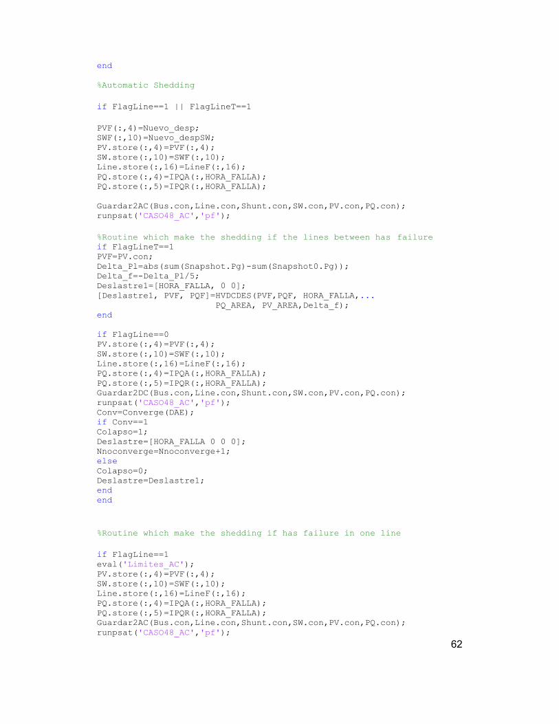
62
end %Automatic Shedding if FlagLine==1 || FlagLineT==1 PVF(:,4)=Nuevo_desp; SWF(:,10)=Nuevo_despSW; PV.store(:,4)=PVF(:,4); SW.store(:,10)=SWF(:,10); Line.store(:,16)=LineF(:,16); PQ.store(:,4)=IPQA(:,HORA_FALLA); PQ.store(:,5)=IPQR(:,HORA_FALLA); Guardar2AC(Bus.con,Line.con,Shunt.con,SW.con,PV.con,PQ.con); runpsat('CASO48_AC','pf'); %Routine which make the shedding if the lines between has failure if FlagLineT==1 PVF=PV.con; Delta_Pl=abs(sum(Snapshot.Pg)-sum(Snapshot0.Pg)); Delta_f=-Delta_Pl/5; Deslastre1=[HORA_FALLA, 0 0]; [Deslastre1, PVF, PQF]=HVDCDES(PVF,PQF, HORA_FALLA,... PQ_AREA, PV_AREA,Delta_f); end if FlagLine==0 PV.store(:,4)=PVF(:,4); SW.store(:,10)=SWF(:,10); Line.store(:,16)=LineF(:,16); PQ.store(:,4)=IPQA(:,HORA_FALLA); PQ.store(:,5)=IPQR(:,HORA_FALLA); Guardar2DC(Bus.con,Line.con,Shunt.con,SW.con,PV.con,PQ.con); runpsat('CASO48_AC','pf'); Conv=Converge(DAE); if Conv==1 Colapso=1; Deslastre=[HORA_FALLA 0 0 0]; Nnoconverge=Nnoconverge+1; else Colapso=0; Deslastre=Deslastre1; end end %Routine which make the shedding if has failure in one line if FlagLine==1 eval('Limites_AC'); PV.store(:,4)=PVF(:,4); SW.store(:,10)=SWF(:,10); Line.store(:,16)=LineF(:,16); PQ.store(:,4)=IPQA(:,HORA_FALLA); PQ.store(:,5)=IPQR(:,HORA_FALLA); Guardar2AC(Bus.con,Line.con,Shunt.con,SW.con,PV.con,PQ.con); runpsat('CASO48_AC','pf');
63
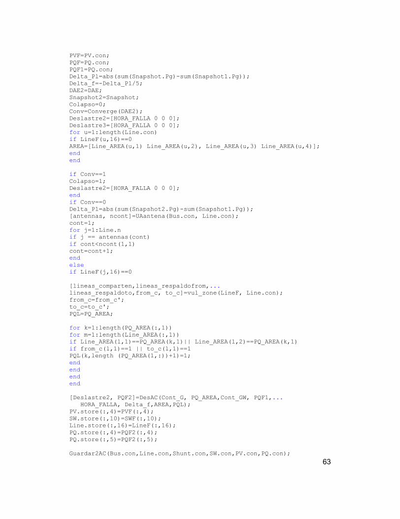
PVF=PV.con; PQF=PQ.con; PQF1=PQ.con; Delta_Pl=abs(sum(Snapshot.Pg)-sum(Snapshot1.Pg)); Delta_f=-Delta_Pl/5; DAE2=DAE; Snapshot2=Snapshot; Colapso=0; Conv=Converge(DAE2); Deslastre2=[HORA_FALLA 0 0 0]; Deslastre3=[HORA_FALLA 0 0 0]; for u=1:length(Line.con) if LineF(u,16)==0 AREA=[Line_AREA(u,1) Line_AREA(u,2), Line_AREA(u,3) Line_AREA(u,4)]; end end if Conv==1 Colapso=1; Deslastre2=[HORA_FALLA 0 0 0]; end if Conv==0 Delta_Pl=abs(sum(Snapshot2.Pg)-sum(Snapshot1.Pg)); [antennas, ncont]=UAantena(Bus.con, Line.con); cont=1; for j=1:Line.n if j == antennas(cont) if cont<ncont(1,1) cont=cont+1; end else if LineF(j,16)==0 [lineas_comparten,lineas_respaldofrom,... lineas_respaldoto,from_c, to_c]=vul_zone(LineF, Line.con); from_c=from_c'; to_c=to_c'; PQL=PQ_AREA; for k=1:length(PQ_AREA(:,1)) for m=1:length(Line_AREA(:,1)) if Line_AREA(l,1)==PQ_AREA(k,1)|| Line_AREA(l,2)==PQ_AREA(k,1) if from_c(l,1)==1 || to_c(l,1)==1 PQL(k,length (PQ_AREA(1,:))+1)=1; end end end end [Deslastre2, PQF2]=DesAC(Cont_G, PQ_AREA,Cont_GW, PQF1,... HORA_FALLA, Delta_f,AREA,PQL); PV.store(:,4)=PVF(:,4); SW.store(:,10)=SWF(:,10); Line.store(:,16)=LineF(:,16); PQ.store(:,4)=PQF2(:,4); PQ.store(:,5)=PQF2(:,5); Guardar2AC(Bus.con,Line.con,Shunt.con,SW.con,PV.con,PQ.con);

64
runpsat('CASO48_AC','pf'); PVF2=PV.con; PQF2=PQ.con; Conv=Converge(DAE); if Conv==1 Colapso=1; Deslastre2=[HORA_FALLA 0 0 0]; end end end end end
PV.store(:,4)=PVF(:,4); SW.store(:,10)=SWF(:,10); Line.store(:,16)=LineF(:,16); PQ.store(:,4)=PQF1(:,4); PQ.store(:,5)=PQF1(:,5); Guardar2AC(Bus.con,Line.con,Shunt.con,SW.con,PV.con,PQ.con); runpsat('CASO48_AC','pf'); PVF2=PV.con; PQF2=PQ.con; Potencia=[HORA_FALLA sum(Snapshot.Pg) sum(Snapshot.Pl)]; %Evaluates the overload in the lines LIMITE_B= Limi_AC*2; LIMITE_A= 1.4*LIMITE_B; if Conv==1 Colapso=1; Deslastre2=[HORA_FALLA 0 0 0]; end if Conv==0; [PIJ PJI QIJ QJI]=FM_FLOWS; s12=PIJ.*PIJ+QIJ.*QIJ; S11=sqrt(s12); s12=PJI.*PJI+QJI.*QJI; S22=sqrt(s12); for g=1:1:length(LineF(:,1)) S13(g,1)=S11(g,1); S23(g,1)=S22(g,1); end SMAX=max(S13,S23); sobrecargasA=sum(SMAX>=LIMITE_A); sobrecargasB=sum(SMAX>=LIMITE_B); if sobrecargasB==0 Colapso=0; Deslastre=Deslastre2; else if sobrecargasA>0 for j=1:Line.n if j == antennas(cont) if cont<ncont(1,1) cont=cont+1; end
else

65
if sobrecargasA>0 [lineas_comparten, lineas_respaldofrom, lineas_respaldoto,... from_c,to_c]=vul_zone(LineF,Line.con); from_c=from_c'; to_c=to_c'; PQL=PQ_AREA;
for k=1:length(PQ_AREA(:,1)) for m=1:length(Line_AREA(:,1)) if Line_AREA(l,1)==PQ_AREA(k,1) ||Line_AREA(l,2)==PQ_AREA(k,1) if from_c(l,1)==1 || to_c(l,1)==1 PQL(k,length(PQ_AREA(1,:))+1)=1; end end end end [Deslastre3,PQF2]=DesAC(Cont_G, PQ_AREA,Cont_GW, PQF, HORA_FALLA,... Delta_f,AREA,PQL); end end end end end if 0<sobrecargasB<sobrecargasA [Deslastre2,PQF2]=Sobrecarga2AC(LineF,SMAX,PQ_AREA,PQF, HORA_FALLA); end end end TempoA=0; TempoB=0; PV.store(:,4)=PVF(:,4); SW.store(:,10)=SWF(:,10); Line.store(:,16)=LineF(:,16); PQ.store(:,4)=PQF2(:,4); PQ.store(:,5)=PQF2(:,5); Guardar2AC(Bus.con,Line.con,Shunt.con,SW.con,PV.con,PQ.con);
runpsat('CASO48_AC','pf'); Conv=Converge(DAE); TempoC(:,1)=PQ1(:,1); TempoC(:,2)=PQ1(:,4)-PQ.con(:,4); TempoC(:,3)=PQ_AREA(:,2); if Colapso==1 for j=1:1:length(PQ_AREA(:,1)) if PQ_AREA(j,2)==1 TempoA=TempoA+PQ.con(j,4); End Nnoconverge= Nnoconverge+1; if PQ_AREA(j,2)==2 TempoB=TempoB+PQ.con(j,4); end end ENSA(HORA_FALLA,YR)=TempoA;

66
ENSB(HORA_FALLA,YR)=TempoB; ENST(HORA_FALLA,YR)=TempoA+TempoA; AENS2=PQ1-PQ.con; end if Colapso==0 if Deslastre1(4) > 0 || Deslastre2(4) > 0 ENSA(HORA_FALLA,YR)=Deslastre1(2)+Deslastre2(2); ENSB(HORA_FALLA,YR)=Deslastre1(3)+Deslastre2(3); ENST(HORA_FALLA,YR)=Deslastre1(4)+Deslastre2(4); AENS=AENS+abs(TempoC(:,2)); AENS2=abs(TempoC(:,2)); Deslastre= Deslastre+1; %Calculates the cost of ENS [CENST2(HORA_FALLA,YR),ENST2(HORA_FALLA,YR)]=ccens(AENS2,... ENST(HORA_FALLA,YR),distc); for k=1:length(PQ_AREA) if PQ_AREA(k,2)==1 AENSA(k)=AENS(k); end if PQ_AREA(k,2)==2 AENSB(k,YR)=AENS(k); end end else ENSA(HORA_FALLA,YR)=0; ENSB(HORA_FALLA,YR)=0; ENST(HORA_FALLA,YR)=0; end end end end end ENSA1(YR)=sum(sum(AENSA)); ENSB1(YR)=sum(sum(AENSB)); [CENST(YR),ENST1(YR)]=ccens(AENS,ENST,distc); CENST(YR)=CENST(YR)/1e6;%Se presenta el CENS en Millones de USD %Estimador (Criterio de parada) if ENST1(YR)~=0 A1=A1+1; ENSE(A1)=ENST1(YR); EST(YR)=std(ENSE)/sqrt(A1); EST2(YR)=std(ENST1)/sqrt(YR); end T(YR)=cputime-Tiempo_0; end Tiempo_1=cputime; TiempoF=Tiempo_1-Tiempo_0;
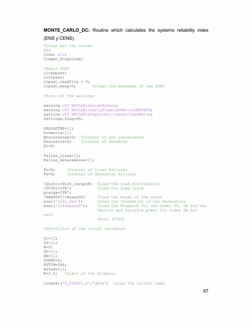
67
MONTE_CARLO_DC: Routine which calculates the systems reliability index
(ENS y CENS).
%Clear all the values clc clear all; Tiempo_0=cputime; %Begin PSAT closepsat; initpsat; clpsat.readfile = 0; clpsat.mesg=0; %Clear the messages of the PSAT %Turn off the warnings warning off MATLAB:divideByZero; warning off MATLAB:nearlySingularMatrixUMFPACK; warning off MATLAB:dispatcher:InexactCaseMatch; Settings.freq=60; DESLASTRE=[]; Potencia=[]; Nnoconverge=0; %Counter of not convergence Deslastre=0; %Counter of shedding A1=0; Fallas_Linea=[]; Fallas_Generadores=[]; FL=0; %Counter of Lines Faliures FG=0; %Counter of Generator Faliures [distc]=dist_carga48; %Load the load distribution [PCYR]=CYR'; %Load the Load curve pcarga=CYR'; [AREASDC]=AreasDC; %Load the Areas of the sytem eval('Info_Gen'); %Load the Iformation of the Generators eval('InfobaseDC'); %Load the Dispatch for the nodes PV, SW and the %Active and reactive power for nodes PQ for each %hour (8760) %Definition of the inital variables U1=[]; U2=[]; N=0; HF=[]; HR=[]; STENS=0; ESTIM=1E6; Estado=[]; K=2.5; %Limit of the stimator runpsat('d_048DC1.m','data') %Load the initial case

68
runpsat ('pf') %run PSAT DAEbase=DAE; Snapshotbase=Snapshot; L_act_in=PQ.con(:,4); %Define the intial Active Power L_react_in=PQ.con(:,5); %Define the intial Reactive Powe eval('Info_Gen'); U1=[]; U2=[]; N=0; HF=[]; HR=[]; STENS=0; AENS=zeros(1,34)'; AENSA=zeros(1,34)'; AENSB=zeros(1,34)'; AENST=zeros(1,34)'; ENSA=zeros(1,34)'; ENSB=zeros(1,34)'; ESTIM=1E6; Estado=[]; ENST=zeros(1,34)'; K=2.5; runpsat('d_048DC1.m','data') runpsat ('pf') DAEbase=DAE; Snapshotbase=Snapshot; %Define the temporal variables. PV1=PV.con; Bus1=Bus.con; PQ1=PQ.con; SW1=SW.con; HVDC1=Hvdc.con; Line1=Line.con; Shunt1=Shunt.con; %Define the areas to the Nodes PV, PQ, SW and Lines [PV_AREA, PQ_AREA, Line_AREA, SW_AREA]=Area(AREASDC,PV1,PQ1,Line1,SW1); %Save the constants that modified the power tranference in the link K1=Hvdc.con(13); K2=Hvdc.con(14); %Load the faliure parameters [PARAM_LINEAS PARAM_GENERADORES PARAM_HVDC]= FallasRTS48DC2; MTTF_LINEAS=PARAM_LINEAS(:,3); % Faliure rates Lines MTTR_LINEAS=PARAM_LINEAS(:,4); % Repair rates Lines

69
MTTF_GENERADORES=PARAM_GENERADORES(:,2); % Faliure rates Geneator MTTR_GENERADORES=PARAM_GENERADORES(:,3); % Repair rates Geneator MTTF_HVDC=PARAM_HVDC(:,3); %Faliure rates HVDC MTTR_HVDC=PARAM_HVDC(:,4); %Repair rates HVDC MTTF=[MTTF_LINEAS; MTTF_GENERADORES; MTTF_HVDC]; MTTR=[MTTR_LINEAS; MTTR_GENERADORES; MTTR_HVDC]; N=length(MTTF); N1=length(MTTF_LINEAS); N2=length(MTTF_GENERADORES); N3=length(MTTF_HVDC(:,1)); %Initilacion Variables YR=1; R=0; ND=0; NTOT=0; A1=0; PQ2=PQ1; L_act_in=PQ.con(:,4); L_react_in=PQ.con(:,5); PQ2=PQ1; eval('InfobaseDC') for YR=1:1:2000 EFALLA=[]; %Faliure elements RFALLA=[]; %Repair elements TFALLA=[]; %Faliure times HFALLA=[]; %Matriz which organize the faliures times F=0; %Counter of the faliure by the realization CF=0; AENS=zeros(1,34)'; AENSA=zeros(1,34)'; AENSB=zeros(1,34)'; AENST=zeros(1,34)'; ENSA=zeros(1,34)'; ENSB=zeros(1,34)'; ENST=zeros(1,34)'; U1=rand(N,1); %Generates random numbers for each elements U2=rand(N,1); %Generates random numbers for each elements HF=-MTTF.*log(U1); %Calculates the failure Hours for each element HF=round(HF); %Round the failure hours %Routine of identification of the failures in the year in the system %determinate the repair time for each one and the reevaluation of the %contingency during the year for R=1:N

70
if HF(R) < 8760 DF=0; %Indicator of end of the contingency evaluation %in the year F=F+1; RFALLA(F,1)=round(-MTTR(R)*log(U2(R))); EFALLA(F,1)=R; TFALLA(F,1)=HF(R); while DF==0 %Is generate another random number if the contingency %it does not present again in the year NHF=round(-MTTF(R)*log(rand)); if NHF<8760 && NHF>TFALLA(F,1)+RFALLA(F,1) F=F+1; RFALLA(F,1)=round(-MTTR(R)*log(rand)); EFALLA(F,1)=R; TFALLA(F,1)=NHF; else DF=1; %It is indicate the end of the cylce end end end end %routine which determinates the vector of the contingencies hours %for the systems for each realization for i=1:F HF=1; for k=TFALLA(i):TFALLA(i)+RFALLA(i) if k > 8760 break else HFALLA(i,HF)=k; HF=HF+1; end end end [iif,iic,s] = find(HFALLA); [s,c]=sort(s); NS=length(s); t2=1; t=1; s2=[]; %Routine which determinates the hours vector of the system with the %respective contingency while t<=NS NC=2; if t==NS s2(t2,1)=s(t); s2(t2,NC)=EFALLA(iif(c(t))); break end if s(t+1)==s(t) s2(t2,1)=s(t); ER=find(s==s(t));

71
for i=1:length(ER) s2(t2,NC)=EFALLA(iif(c(ER(i)))); NC=NC+1; end t=t+length(ER); else s2(t2,1)=s(t); s2(t2,NC)=EFALLA(iif(c(t))); t=t+1; end t2=t2+1; end NTOT=NTOT+length(s2(:,1)); for i=1:length(s2(:,1)) HORA_FALLA=s2(i,1); EF=find(s2(i,:)); FlagLineT=0; %Flag indicates faliure in the lines that interconnect %the areas FlagLine=0; %Flag indicates faliure in a line Flag_Gen=0; %Flag indicates faliure in the generators Flag_HVDC1=0; %Flag indicates faliure in the HVDC link Falg_HVDC2=0; %Flag indicates faliure 0f 50% in the HVDC link %Load the information of the base case for the failure hour PV.store(:,4)=IPV(:,HORA_FALLA); PQ.store(:,4)=IPQA(:,HORA_FALLA); PQ.store(:,5)=IPQR(:,HORA_FALLA); SW.store(:,10)=ISW(:,HORA_FALLA); Despacho_Disponible=IPV(:,HORA_FALLA); %Save the initial information Guardar2DC(Bus1,Line1,Shunt1,SW.con,PV.con,PQ.con,HVDC1); %Run Power Flow for the Case Base runpsat('CASO48_DC','pf'); DAE1=DAE; Snapshot1=Snapshot; %calculates the initial Flow in the lines [PIJ1 PJI1 QIJ1 QJI1]=FM_FLOWS; %Define the initial temp variables PV3=PV.con; PQ3=PQ.con; LineF=Line.con; SupplyF=Supply1; HVDCF=HVDC1; FallasL=[]; Cont_GW=[0 0 0]; Cont_G=[0 0 0]; for j=1:length(EF)-1 FR=s2(i,j+1); if FR<=N1 LineF(s2(i,j+1),16)=0; FL=FL+1; FlagLine=1;

72
FallasL(c,1)=LineF(s2(i,j+1),1); FallasL(c,2)=LineF(s2(i,j+1),2); FallasL(c,3)=Line_AREA(s2(i,j+1),3); FallasL(c,4)=Line_AREA(s2(i,j+1),4); FallasL(c,5)=0; elseif N1<FR<=(N1+N2) GR=s2(i,j+1)-N1; SupplyF(GR,20)=0; FG=FG+1; Flag_Gen=1; elseif (N1+N2)<FR<=N HVR=s2(i,j+1)-N1-N2; if HVR==1 HVDCF(1,29)=0; Flag_HVDC1=1; Flag_HVDC2=0; elseif HVR==2 HVDCF(1,29)=1; HVDCF(1,13)=K1/2; HVDCF(1,13)=K2/2; Flag_HVDC2=1; Flag_HVDC1=0; elseif HVR==3 HVDC1(1,29)=1; HVDC1(1,13)=K1/2; HVDC1(1,14)=K2/2; Hvdc.store(:,[13 14 29])=HVDC1(:,[13 14 29]); PV.store(:,4)=PV3(:,4); PQ.store(:,[4 5])=PQ3(:,[4 5]); Guardar2DC(Bus.con,Line.con,Shunt.con,SW.con,PV.con,PQ.con,Hvdc.con); runpsat('CASO48_DC','pf'); DAE1=DAE; Snapshot1=Snapshot; HVDCF(1,29)=0; Flag_HVDC2=1; Flag_HVDC1=1; end end end %modified the information of PV, SW nodes taking in account the %contingencies [GenF, GenSW1F]=PV_FALLA(SupplyF, Gen, UGEN, UGenSW, GenSW); %Calculates de dispatch for m=1:1:length(Despacho_Disponible(:,1)) if Gen_disp(m) >= sum(Despacho_Disponible(m,2:... length(Despacho_Disponible(1,:)))); Nuevo_desp(m)=sum(Despacho_Disponible(m,2:.... length(Despacho_Disponible(1,:)))); end if Gen_disp < sum(Despacho_Disponible(m,2:... length(Despacho_Disponible(1,:))));

73
Nuevo_desp(m)=Gen_disp(m); FlagLine=1; Cont_G(f,1)=Gen(m,1); Cont_G(f,2)=PV_AREA(m,2); f=f+1; end end for m=1:1:length(GenSW1F(:,1)) if Gen_disSW(m) >= sum(GenSW1F(m,2:length(GenSW1F(1,:)))); Nuevo_despSW(m)=sum(GenSW1F(m,2:length(GenSW1F(1,:)))); end if Gen_disSW(m) < sum(GenSW1F(m,2:length(GenSW1F(1,:)))); Nuevo_despSW(m)=Gen_disSW(m); FlagLine=1; Cont_GW(s,1)=GenSW1(m,1); Cont_GW(s,2)=SW_AREA(m,1); s=s+1; end end PVF=PV1; SWF=SW1;
for l=1:length(LineF(:,1)) if Line_AREA(l,3)==1 && Line_AREA(l,4)==2 && LineF(l,16)==0 FlagLineT=1; end end %Automatic Shedding if FlagLine==1 || Flag_HVDC1==1 || FlagLineT==1 PVF(:,4)=Nuevo_desp; SWF(:,10)=Nuevo_despSW; PV.store(:,4)=PVF(:,4); SW.store(:,10)=SWF(:,10); Line.store(:,16)=LineF(:,16); PQ.store(:,4)=IPQA(:,HORA_FALLA); PQ.store(:,5)=IPQR(:,HORA_FALLA); Hvdc.store(:,29)=HVDCF(:,29); Guardar2DC(Bus.con,Line.con,Shunt.con,SW.con,PV.con,PQ.con,Hvdc.con); runpsat('CASO48_DC','pf'); %Routine which make the shedding if the lines between has %failure if Flag_HVDC1==1 || FlagLineT==1 [AREASDC]=AreasDC; PVF=PV.con; Delta_Pl=abs(sum(Snapshot.Pg)-sum(Snapshot0.Pg)); Delta_f=-Delta_Pl/5; Deslastre1=[HORA_FALLA, 0 0]; [Deslastre1,PVF,PQF]=HVDCDES(PVF,PQF,HORA_FALLA,PQ_AREA,PV_AREA,Delta_f); end

74
if FlagLine==0 PV.store(:,4)=PVF(:,4); SW.store(:,10)=SWF(:,10); Line.store(:,16)=LineF(:,16); PQ.store(:,4)=IPQA(:,HORA_FALLA); PQ.store(:,5)=IPQR(:,HORA_FALLA); Hvdc.store(:,29)=HVDCF(:,29); Guardar2DC(Bus.con,Line.con,Shunt.con,SW.con,PV.con,PQ.con,Hvdc.con); runpsat('CASO48_DC','pf'); Conv=Converge(DAE); if Conv==1 Colapso=1; Deslastre1=[HORA_FALLA 0 0 0]; else Colapso=0; Deslastre=Deslastre1; end end
%Routine which make the shedding if has failure in one line if FlagLine==1 eval('Limites_DC'); PV.store(:,4)=PVF(:,4); SW.store(:,10)=SWF(:,10); Line.store(:,16)=LineF(:,16); PQ.store(:,4)=IPQA(:,HORA_FALLA); PQ.store(:,5)=IPQR(:,HORA_FALLA); Hvdc.store(:,29)=HVDCF(:,29); Guardar2DC(Bus.con,Line.con,Shunt.con,SW.con,PV.con,PQ.con,Hvdc.con); runpsat('CASO48_DC','pf'); if LineF(u,16)==0 AREA=[Line_AREA(u,1) Line_AREA(u,2), Line_AREA(u,3) Line_AREA(u,4)]; end end if Conv==1 Colapso=1; Deslastre2=[HORA_FALLA 0 0 0]; end if Conv==0 Delta_Pl=abs(sum(Snapshot2.Pg)-sum(Snapshot1.Pg)); [antennas, ncont]=UAantena(Bus.con, Line.con); cont=1; for j=1:Line.n if j == antennas(cont) if cont<ncont(1,1) cont=cont+1; end else if LineF(j,16)==0 [lineas_comparten,lineas_respaldofrom,... lineas_respaldoto,from_c, to_c]=vul_zone(LineF, Line.con); from_c=from_c'; to_c=to_c'; PQL=PQ_AREA;

75
for k=1:length(PQ_AREA(:,1)) for m=1:length(Line_AREA(:,1)) if Line_AREA(l,1)==PQ_AREA(k,1)|| Line_AREA(l,2)==PQ_AREA(k,1) if from_c(l,1)==1 || to_c(l,1)==1 PQL(k,length (PQ_AREA(1,:))+1)=1; end end end end [Deslastre2, PQF2]=DesAC(Cont_G, PQ_AREA,Cont_GW, PQF1,... HORA_FALLA, Delta_f,AREA,PQL); PV.store(:,4)=PVF(:,4); SW.store(:,10)=SWF(:,10); Line.store(:,16)=LineF(:,16); PQ.store(:,4)=PQF2(:,4); PQ.store(:,5)=PQF2(:,5); Guardar2DC(Bus.con,Line.con,Shunt.con,SW.con,PV.con,PQ.con,Hvdc.con); runpsat('CASO48_DC','pf'); PVF2=PV.con; PQF2=PQ.con; Conv=Converge(DAE); if Conv==1 Colapso=1; Deslastre2=[HORA_FALLA 0 0 0]; end end end end end
PV.store(:,4)=PVF(:,4); SW.store(:,10)=SWF(:,10); Line.store(:,16)=LineF(:,16); PQ.store(:,4)=PQF1(:,4); PQ.store(:,5)=PQF1(:,5); Guardar2DC(Bus.con,Line.con,Shunt.con,SW.con,PV.con,PQ.con,Hvdc.con); runpsat('CASO48_DC','pf'); PVF2=PV.con; PQF2=PQ.con; Potencia=[HORA_FALLA sum(Snapshot.Pg) sum(Snapshot.Pl)]; %Evaluates the overload in the lines LIMITE_B= Lim_DC*2; LIMITE_A= 1.4*LIMITE_B; if Conv==1 Colapso=1; Deslastre2=[HORA_FALLA 0 0 0]; end if Conv==0; [PIJ PJI QIJ QJI]=FM_FLOWS; s12=PIJ.*PIJ+QIJ.*QIJ; S11=sqrt(s12); s12=PJI.*PJI+QJI.*QJI;

76
S22=sqrt(s12); for g=1:1:length(LineF(:,1)) S13(g,1)=S11(g,1); S23(g,1)=S22(g,1); end SMAX=max(S13,S23); sobrecargasA=sum(SMAX>=LIMITE_A); sobrecargasB=sum(SMAX>=LIMITE_B); if sobrecargasB==0 Colapso=0; Deslastre=Deslastre2; else if sobrecargasA>0 for j=1:Line.n if j == antennas(cont) if cont<ncont(1,1) cont=cont+1; end
else if sobrecargasA>0 [lineas_comparten, lineas_respaldofrom, lineas_respaldoto,... from_c,to_c]=vul_zone(LineF,Line.con); from_c=from_c'; to_c=to_c'; PQL=PQ_AREA;
for k=1:length(PQ_AREA(:,1)) for m=1:length(Line_AREA(:,1)) if Line_AREA(l,1)==PQ_AREA(k,1) ||Line_AREA(l,2)==PQ_AREA(k,1) if from_c(l,1)==1 || to_c(l,1)==1 PQL(k,length(PQ_AREA(1,:))+1)=1; end end end end [Deslastre3,PQF2]=DesAC(Cont_G, PQ_AREA,Cont_GW, PQF, HORA_FALLA,... Delta_f,AREA,PQL); end end end end end if 0<sobrecargasB<sobrecargasA [Deslastre2,PQF2]=Sobrecarga2AC(LineF,SMAX,PQ_AREA,PQF, HORA_FALLA); end end end TempoA=0; TempoB=0; PV.store(:,4)=PVF(:,4); SW.store(:,10)=SWF(:,10); Line.store(:,16)=LineF(:,16); PQ.store(:,4)=PQF2(:,4); PQ.store(:,5)=PQF2(:,5);

77
Guardar2DC(Bus.con,Line.con,Shunt.con,SW.con,PV.con,PQ.con,Hvdc.con);
runpsat('CASO48_DC','pf'); Conv=Converge(DAE); TempoC(:,1)=PQ1(:,1); TempoC(:,2)=PQ1(:,4)-PQ.con(:,4); TempoC(:,3)=PQ_AREA(:,2); if Colapso==1 for j=1:1:length(PQ_AREA(:,1)) if PQ_AREA(j,2)==1 TempoA=TempoA+PQ.con(j,4); End Nnoconverge= Nnoconverge+1; if PQ_AREA(j,2)==2 TempoB=TempoB+PQ.con(j,4); end end ENSA(HORA_FALLA,YR)=TempoA; ENSB(HORA_FALLA,YR)=TempoB; ENST(HORA_FALLA,YR)=TempoA+TempoA; AENS2=PQ1-PQ.con; end if Colapso==0 if Deslastre1(4) > 0 || Deslastre2(4) > 0 ENSA(HORA_FALLA,YR)=Deslastre1(2)+Deslastre2(2); ENSB(HORA_FALLA,YR)=Deslastre1(3)+Deslastre2(3); ENST(HORA_FALLA,YR)=Deslastre1(4)+Deslastre2(4); AENS=AENS+abs(TempoC(:,2)); AENS2=abs(TempoC(:,2)); Deslastre= Deslastre+1; %Calculates the cost of ENS [CENST2(HORA_FALLA,YR),ENST2(HORA_FALLA,YR)]=ccens(AENS2,... ENST(HORA_FALLA,YR),distc); for k=1:length(PQ_AREA) if PQ_AREA(k,2)==1 AENSA(k)=AENS(k); end if PQ_AREA(k,2)==2 AENSB(k,YR)=AENS(k); end end else ENSA(HORA_FALLA,YR)=0; ENSB(HORA_FALLA,YR)=0; ENST(HORA_FALLA,YR)=0; end end end end end
78
ENSA1(YR)=sum(sum(AENSA)); ENSB1(YR)=sum(sum(AENSB)); [CENST(YR),ENST1(YR)]=ccens(AENS,ENST,distc); CENST(YR)=CENST(YR)/1e6;%Se presenta el CENS en Millones de USD %Estimador (Criterio de parada) if ENST1(YR)~=0 A1=A1+1; ENSE(A1)=ENST1(YR); EST(YR)=std(ENSE)/sqrt(A1); EST2(YR)=std(ENST1)/sqrt(YR); end T(YR)=cputime-Tiempo_0; end Tiempo_1=cputime; TiempoF=Tiempo_1-Tiempo_0;
Area: Routine that assigns the area to nodes PQ, PV and the lines.
function [PV_AREA,PQ_AREA,Line_AREA,SW_AREA]=Area(AREASDC,PV1,PQ1, Line1,SW1) for i=1:1:length(PV1(:,1)) for j=1:1:length(AREASDC(:,1)) if PV1(i,1)==AREASDC(j,1); PV_AREA(i,1)=PV1(i,1); PV_AREA(i,2)=AREASDC(j,2); end end end for i=1:1:length(PQ1(:,1)) for j=1:1:length(AREASDC(:,1)) if PQ1(i,1)==AREASDC(j,1); PQ_AREA(i,1)=PQ1(i,1); PQ_AREA(i,2)=AREASDC(j,2); end end end for i=1:1:length(Line1(:,1)) for j=1:1:length(AREASDC(:,1)) if Line1(i,1)==AREASDC(j,1); Line_AREA(i,1)=Line1(i,1); Line_AREA(i,3)=AREASDC(j,2); end end end for i=1:1:length(Line1(:,1)) for j=1:1:length(AREASDC(:,1)) if Line1(i,2)==AREASDC(j,1); Line_AREA(i,2)=Line1(i,2); Line_AREA(i,4)=AREASDC(j,2);

79
end end end for i=1:1:length(SW1(:,1)) for j=1:1:length(AREASDC(:,1)) if SW1(i,1)==AREASDC(j,1); SW_AREA(i,1)=SW1(i,2); SW_AREA(i,4)=AREASDC(j,2); end end end end
DESHVDC: Routine which make the shedding in Area 2 and loss generation in
Area 1.
function [Deslastre, PVF, PQF]=HVDCDES(PVF,PQF, HORA_FALLA, PQ_AREA, PV_AREA,Delta_f) Des=[HORA_FALLA 0 0 0]; Deslastre=[HORA_FALLA 0 0 0]; if Delta_f <= 0 if (Delta_f <= 0)&&(Delta_f > -0.2) C_Des=0.005; P_Des=0.005; for i=1:length(PV_AREA(:,1)) if (PV_AREA(i,2)==1) if PVF(i,4)<P_Des Des(2)=Des(2)+PQF(i,4); PVF(i,4)=0; end if PVF(i,4)>=P_Des Des(2)=Des(2)+P_Des; PVF(i,4)=PVF(i,4)-P_Des; end end end for i=1:length(PQ_AREA(:,1)) if (PQ_AREA(i,2)==2) if PQF(i,4)<C_Des Des(3)=Des(3)+PQF(i,4); PQF(i,5)=0; PQF(i,4)=0; end if PQF(i,4)>=C_Des Des(3)=Des(3)+C_Des; theta=atan(PQF(i,5)/PQF(i,4)); PQF(i,4)=PQF(i,4)-C_Des; PQF(i,5)=PQF(i,4)*tan(theta); end end end

80
end if (Delta_f <= -0.2)&&(Delta_f > -0.4) C_Des=0.01; P_Des=0.01; for i=1:length(PV_AREA(:,1)) if (PV_AREA(i,2)==1) if PVF(i,4)<P_Des Des(2)=Des(2)+PQF(i,4); PVF(i,4)=0; end if PVF(i,4)>=P_Des Des(2)=Des(2)+P_Des; PVF(i,4)=PVF(i,4)-P_Des; end end end for i=1:length(PQ_AREA(:,1)) if (PQ_AREA(i,2)==2) if PQF(i,4)<C_Des Des(3)=Des(3)+PQF(i,4); PQF(i,5)=0; PQF(i,4)=0; end if PQF(i,4)>=C_Des Des(3)=Des(3)+C_Des; theta=atan(PQF(i,5)/PQF(i,4)); PQF(i,4)=PQF(i,4)-C_Des; PQF(i,5)=PQF(i,4)*tan(theta); end end end end if (Delta_f <= -0.4)&&(Delta_f > -0.6) C_Des=0.015; P_Des=0.015; for i=1:length(PV_AREA(:,1)) if (PV_AREA(i,2)==1) if PVF(i,4)<P_Des Des(2)=Des(2)+PQF(i,4); PVF(i,4)=0; end if PVF(i,4)>=P_Des Des(2)=Des(2)+P_Des; PVF(i,4)=PVF(i,4)-P_Des; end end end for i=1:length(PQ_AREA(:,1)) if (PQ_AREA(i,2)==2) if PQF(i,4)<C_Des Des(3)=Des(3)+PQF(i,4); PQF(i,5)=0; PQF(i,4)=0; end if PQF(i,4)>=C_Des Des(3)=Des(3)+C_Des; theta=atan(PQF(i,5)/PQF(i,4)); PQF(i,4)=PQF(i,4)-C_Des; PQF(i,5)=PQF(i,4)*tan(theta);

81
end end end end if (Delta_f <= -0.6)&&(Delta_f > -0.8) C_Des=0.020; P_Des=0.020; for i=1:length(PV_AREA(:,1)) if (PV_AREA(i,2)==1) if PVF(i,4)<P_Des Des(2)=Des(2)+PQF(i,4); PVF(i,4)=0; end if PVF(i,4)>=P_Des Des(2)=Des(2)+P_Des; PVF(i,4)=PVF(i,4)-P_Des; end end end for i=1:length(PQ_AREA(:,1)) if (PQ_AREA(i,2)==2) if PQF(i,4)<C_Des Des(3)=Des(3)+PQF(i,4); PQF(i,5)=0; PQF(i,4)=0; end if PQF(i,4)>=C_Des Des(3)=Des(3)+C_Des; theta=atan(PQF(i,5)/PQF(i,4)); PQF(i,4)=PQF(i,4)-C_Des; PQF(i,5)=PQF(i,4)*tan(theta); end end end end if (Delta_f <= -0.8)&&(Delta_f > -1.0) C_Des=0.025; P_Des=0.025; for i=1:length(PV_AREA(:,1)) if (PV_AREA(i,2)==1) if PVF(i,4)<P_Des Des(2)=Des(2)+PQF(i,4); PVF(i,4)=0; end if PVF(i,4)>=P_Des Des(2)=Des(2)+P_Des; PVF(i,4)=PVF(i,4)-P_Des; end end end for i=1:length(PQ_AREA(:,1)) if (PQ_AREA(i,2)==2) if PQF(i,4)<C_Des Des(3)=Des(3)+PQF(i,4); PQF(i,5)=0; PQF(i,4)=0; end if PQF(i,4)>=C_Des Des(3)=Des(3)+C_Des;
82
theta=atan(PQF(i,5)/PQF(i,4)); PQF(i,4)=PQF(i,4)-C_Des; PQF(i,5)=PQF(i,4)*tan(theta); end end end end if (Delta_f <= -1.0)&&(Delta_f > -1.2) C_Des=0.03; P_Des=0.03; for i=1:length(PV_AREA(:,1)) if (PV_AREA(i,2)==1) if PVF(i,4)<P_Des Des(2)=Des(2)+PQF(i,4); PVF(i,4)=0; end if PVF(i,4)>=P_Des Des(2)=Des(2)+P_Des; PVF(i,4)=PVF(i,4)-P_Des; end end end for i=1:length(PQ_AREA(:,1)) if (PQ_AREA(i,2)==2) if PQF(i,4)<C_Des Des(3)=Des(3)+PQF(i,4); PQF(i,5)=0; PQF(i,4)=0; end if PQF(i,4)>=C_Des Des(3)=Des(3)+C_Des; theta=atan(PQF(i,5)/PQF(i,4)); PQF(i,4)=PQF(i,4)-C_Des; PQF(i,5)=PQF(i,4)*tan(theta); end end end end if (Delta_f <= -1.2)&&(Delta_f > -1.4) C_Des=0.035; P_Des=0.035; for i=1:length(PV_AREA(:,1)) if (PV_AREA(i,2)==1) if PVF(i,4)<P_Des Des(2)=Des(2)+PQF(i,4); PVF(i,4)=0; end if PVF(i,4)>=P_Des Des(2)=Des(2)+P_Des; PVF(i,4)=PVF(i,4)-P_Des; end end end for i=1:length(PQ_AREA(:,1)) if (PQ_AREA(i,2)==2) if PQF(i,4)<C_Des Des(3)=Des(3)+PQF(i,4); PQF(i,5)=0; PQF(i,4)=0;

83
end if PQF(i,4)>=C_Des Des(3)=Des(3)+C_Des; theta=atan(PQF(i,5)/PQF(i,4)); PQF(i,4)=PQF(i,4)-C_Des; PQF(i,5)=PQF(i,4)*tan(theta); end end end end if (Delta_f <= -1.4)&&(Delta_f > -1.6) C_Des=0.04; P_Des=0.04; for i=1:length(PV_AREA(:,1)) if (PV_AREA(i,2)==1) if PVF(i,4)<P_Des Des(2)=Des(2)+PQF(i,4); PVF(i,4)=0; end if PVF(i,4)>=P_Des Des(2)=Des(2)+P_Des; PVF(i,4)=PVF(i,4)-P_Des; end end end for i=1:length(PQ_AREA(:,1)) if (PQ_AREA(i,2)==2) if PQF(i,4)<C_Des Des(3)=Des(3)+PQF(i,4); PQF(i,5)=0; PQF(i,4)=0; end if PQF(i,4)>=C_Des Des(3)=Des(3)+C_Des; theta=atan(PQF(i,5)/PQF(i,4)); PQF(i,4)=PQF(i,4)-C_Des; PQF(i,5)=PQF(i,4)*tan(theta); end end end end if (Delta_f <= -1.6)&&(Delta_f > -1.8) C_Des=0.045; P_Des=0.045; for i=1:length(PV_AREA(:,1)) if (PV_AREA(i,2)==1) if PVF(i,4)<P_Des Des(2)=Des(2)+PQF(i,4); PVF(i,4)=0; end if PVF(i,4)>=P_Des Des(2)=Des(2)+P_Des; PVF(i,4)=PVF(i,4)-P_Des; end end end for i=1:length(PQ_AREA(:,1)) if (PQ_AREA(i,2)==2) if PQF(i,4)<C_Des

84
Des(3)=Des(3)+PQF(i,4); PQF(i,5)=0; PQF(i,4)=0; end if PQF(i,4)>=C_Des Des(3)=Des(3)+C_Des; theta=atan(PQF(i,5)/PQF(i,4)); PQF(i,4)=PQF(i,4)-C_Des; PQF(i,5)=PQF(i,4)*tan(theta); end end end end if (Delta_f <= -1.8)&&(Delta_f > -2) C_Des=0.050; P_Des=0.050; for i=1:length(PV_AREA(:,1)) if (PV_AREA(i,2)==1) if PVF(i,4)<P_Des Des(2)=Des(2)+PQF(i,4); PVF(i,4)=0; end if PVF(i,4)>=P_Des Des(2)=Des(2)+P_Des; PVF(i,4)=PVF(i,4)-P_Des; end end end for i=1:length(PQ_AREA(:,1)) if (PQ_AREA(i,2)==2) if PQF(i,4)<C_Des Des(3)=Des(3)+PQF(i,4); PQF(i,5)=0; PQF(i,4)=0; end if PQF(i,4)>=C_Des Des(3)=Des(3)+C_Des; theta=atan(PQF(i,5)/PQF(i,4)); PQF(i,4)=PQF(i,4)-C_Des; PQF(i,5)=PQF(i,4)*tan(theta); end end end end if (Delta_f <= -2) C_Des=0.055; P_Des=0.055; for i=1:length(PV_AREA(:,1)) if (PV_AREA(i,2)==1) if PVF(i,4)<P_Des Des(2)=Des(2)+PQF(i,4); PVF(i,4)=0; end if PVF(i,4)>=P_Des Des(2)=Des(2)+P_Des; PVF(i,4)=PVF(i,4)-P_Des; end end end

85
for i=1:length(PQ_AREA(:,1)) if (PQ_AREA(i,2)==2) if PQF(i,4)<C_Des Des(3)=Des(3)+PQF(i,4); PQF(i,5)=0; PQF(i,4)=0; end if PQF(i,4)>=C_Des Des(3)=Des(3)+C_Des; theta=atan(PQF(i,5)/PQF(i,4)); PQF(i,4)=PQF(i,4)-C_Des; PQF(i,5)=PQF(i,4)*tan(theta); end end end end Deslastre=[HORA_FALLA Des(2) Des(3) (Des(2)+Des(3))]; end
CONVERGE: Routine which determinates if the system does not converge.
function [conv]=Converge(DAE) err_max = norm(DAE.g,inf); if err_max>1.0000e-003 conv=1; else conv=0; end
DESAC: Routine which calculate the automatic shedding in case that the supply
is less than the load.
function [Deslastre2, PQF2]=DesAC(Cont_G,PQ_AREA,Cont_GW, PQF, HORA_FALLA, Delta_f,AREA,PQL) PQF2=PQF; Hora_Falla=HORA_FALLA; Des=[Hora_Falla 0 0 0]; Deslastre2=[Hora_Falla 0 0 0]; Colapso=0; Area=[0 0]; D1=0; D2=0; m=0; Area1=sum(sum(ismember(AREA(:,2),1)))+sum(ismember(Cont_G(:,2),1))+sum(ismember(Cont_GW(:,2),1)); Area2=sum(sum(ismember(AREA(:,2),2)))+sum(ismember(Cont_G(:,2),2))+sum(ismember(Cont_GW(:,2),1)); if (Area1>=Area2); D1=1;

86
end if (Area2>=Area1) D2=2; end if Delta_f <= 0 if (Delta_f <= 0)&&(Delta_f > -0.2) C_Des=0.095; if D1==1 for m=1:34 if (PQ_AREA(m,2)==1) && PQL(m,length(PQ_AREA(1,:))+1)==1 && m<=34 if PQF2(m,4)<C_Des Des(2)=Des(2)+PQF2(m,4); PQF2(m,4)=0; PQF2(m,5)=0; end if PQF(m,4)>=C_Des theta=atan(PQF(m,5)/PQF(m,4)); PQF2(m,4)=PQF2(m,4)-C_Des; PQF2(m,5)=tan(theta)*PQF2(m,4); Des(2)=Des(2)+C_Des; end end end end if D2==2 for m=1:34 if (PQ_AREA(m,2)==2) && PQL(m,length(PQ_AREA(1,:))+1)==1 && m<=34 if PQF2(m,4)<C_Des Des(3)=Des(3)+PQF2(m,4); PQF2(m,5)=0; PQF2(m,4)=0; end if PQF2(m,4)>=C_Des Des(3)=Des(3)+C_Des; theta=atan(PQF2(m,5)/PQF2(m,4)); PQF2(m,4)=PQF2(m,4)-C_Des; PQF2(m,5)=PQF2(m,4)*tan(theta); end end end end end if (Delta_f <= -0.2)&&(Delta_f > -0.4) C_Des=0.01; if D1==1 for m=1:34 if (PQ_AREA(m,2)==1) && PQL(m,length(PQ_AREA(1,:))+1)==1 && m<=34 if PQF2(m,4)<C_Des Des(2)=Des(2)+PQF2(m,4); PQF2(m,4)=0; PQF2(m,5)=0; end if PQF2(m,4)>=C_Des
87
theta=atan(PQF(m,5)/PQF(m,4)); PQF2(m,4)=PQF2(m,4)-C_Des; PQF2(m,5)=tan(theta)*PQF2(m,4); Des(2)=Des(2)+C_Des; end end end end if D2==2 for m=1:34 if (PQ_AREA(m,2)==2) && PQL(m,length(PQ_AREA(1,:))+1)==1 && m<=34 if PQF2(m,4)<C_Des Des(3)=Des(3)+PQF2(m,4); PQF2(m,5)=0; PQF2(m,4)=0; end if PQF2(m,4)>=C_Des Des(3)=Des(3)+C_Des; theta=atan(PQF2(m,5)/PQF2(m,4)); PQF2(m,4)=PQF2(m,4)-C_Des; PQF2(m,5)=PQF2(m,4)*tan(theta); end end end end end if (Delta_f <= -0.4)&&(Delta_f > -0.6) C_Des=0.015; if D1==1 for m=1:34 if (PQ_AREA(m,2)==1) && PQL(m,length(PQ_AREA(1,:))+1)==1 && m<=34 if PQF2(m,4)<C_Des Des(2)=Des(2)+PQF2(m,4); PQF2(m,4)=0; PQF2(m,5)=0; end if PQF2(m,4)>=C_Des theta=atan(PQF(m,5)/PQF(m,4)); PQF2(m,4)=PQF2(m,4)-C_Des; PQF2(m,5)=tan(theta)*PQF2(m,4); Des(2)=Des(2)+C_Des; end end end end if D2==2 for m=1:34 if (PQ_AREA(m,2)==2) && PQL(m,length(PQ_AREA(1,:))+1)==1 && m<=34 if PQF2(m,4)<C_Des Des(3)=Des(3)+PQF2(m,4); PQF2(m,5)=0; PQF2(m,4)=0; end if PQF2(m,4)>=C_Des Des(3)=Des(3)+C_Des; theta=atan(PQF2(m,5)/PQF2(m,4));
88
PQF2(m,4)=PQF2(m,4)-C_Des; PQF2(m,5)=PQF2(m,4)*tan(theta); end end end end end if (Delta_f <= -0.6)&&(Delta_f > -0.8) C_Des=0.020; if D1==1 for m=1:34 if (PQ_AREA(m,2)==1) && PQL(m,length(PQ_AREA(1,:))+1)==1 && m<=34 if PQF2(m,4)<C_Des Des(2)=Des(2)+PQF2(m,4); PQF2(m,4)=0; PQF2(m,5)=0; end if PQF2(m,4)>=C_Des theta=atan(PQF(m,5)/PQF(m,4)); PQF2(m,4)=PQF2(m,4)-C_Des; PQF2(m,5)=tan(theta)*PQF2(m,4); Des(2)=Des(2)+C_Des; end end end end if D2==2 for m=1:34 if (PQ_AREA(m,2)==2) && PQL(m,length(PQ_AREA(1,:))+1)==1 && m<=34 if PQF2(m,4)<C_Des Des(3)=Des(3)+PQF2(m,4); PQF2(m,5)=0; PQF2(m,4)=0; end if PQF2(m,4)>=C_Des Des(3)=Des(3)+C_Des; theta=atan(PQF2(m,5)/PQF2(m,4)); PQF2(m,4)=PQF2(m,4)-C_Des; PQF2(m,5)=PQF2(m,4)*tan(theta); end end end end end if (Delta_f <= -0.8)&&(Delta_f > -1.0) C_Des=0.025; if D1==1 for m=1:34 if (PQ_AREA(m,2)==1) && PQL(m,length(PQ_AREA(1,:))+1)==1 && m<=34 if PQF2(m,4)<C_Des Des(2)=Des(2)+PQF2(m,4); PQF2(m,4)=0; PQF2(m,5)=0; end if PQF2(m,4)>=C_Des theta=atan(PQF(m,5)/PQF(m,4));

89
PQF2(m,4)=PQF2(m,4)-C_Des; PQF2(m,5)=tan(theta)*PQF2(m,4); Des(2)=Des(2)+C_Des; end end end end if D2==2 for m=1:34 if (PQ_AREA(m,2)==2) && PQL(m,length(PQ_AREA(1,:))+1)==1 && m<=34 if PQF2(m,4)<C_Des Des(3)=Des(3)+PQF2(m,4); PQF2(m,5)=0; PQF2(m,4)=0; end if PQF2(m,4)>=C_Des Des(3)=Des(3)+C_Des; theta=atan(PQF2(m,5)/PQF2(m,4)); PQF2(m,4)=PQF2(m,4)-C_Des; PQF2(m,5)=PQF2(m,4)*tan(theta); end end end end end if (Delta_f <= -1.0)&&(Delta_f > -1.2) C_Des=0.03; if D1==1 for m=1:34 if (PQ_AREA(m,2)==1) && PQL(m,length(PQ_AREA(1,:))+1)==1 && m<=34 if PQF2(m,4)<C_Des Des(2)=Des(2)+PQF2(m,4); PQF2(m,4)=0; PQF2(m,5)=0; end if PQF2(m,4)>=C_Des theta=atan(PQF(m,5)/PQF(m,4)); PQF2(m,4)=PQF2(m,4)-C_Des; PQF2(m,5)=tan(theta)*PQF2(m,4); Des(2)=Des(2)+C_Des; end end end end if D2==2 for m=1:34 if (PQ_AREA(m,2)==2) && PQL(m,length(PQ_AREA(1,:))+1)==1 && m<=34 if PQF2(m,4)<C_Des Des(3)=Des(3)+PQF2(m,4); PQF2(m,5)=0; PQF2(m,4)=0; end if PQF2(m,4)>=C_Des Des(3)=Des(3)+C_Des; theta=atan(PQF2(m,5)/PQF2(m,4)); PQF2(m,4)=PQF2(m,4)-C_Des;

90
PQF2(m,5)=PQF2(m,4)*tan(theta); end end end end end if (Delta_f <= -1.2)&&(Delta_f > -1.4) C_Des=0.035; if D1==1 for m=1:34 if (PQ_AREA(m,2)==1) && PQL(m,length(PQ_AREA(1,:))+1)==1 && m<=34 if PQF2(m,4)<C_Des Des(2)=Des(2)+PQF2(m,4); PQF2(m,4)=0; PQF2(m,5)=0; end if PQF2(m,4)>=C_Des theta=atan(PQF(m,5)/PQF(m,4)); PQF2(m,4)=PQF2(m,4)-C_Des; PQF2(m,5)=tan(theta)*PQF2(m,4); Des(2)=Des(2)+C_Des; end end end end if D2==2 for m=1:34 if (PQ_AREA(m,2)==2) && PQL(m,length(PQ_AREA(1,:))+1)==1 && m<=34 if PQF2(m,4)<C_Des Des(3)=Des(3)+PQF2(m,4); PQF2(m,5)=0; PQF2(m,4)=0; end if PQF2(m,4)>=C_Des Des(3)=Des(3)+C_Des; theta=atan(PQF2(m,5)/PQF2(m,4)); PQF2(m,4)=PQF2(m,4)-C_Des; PQF2(m,5)=PQF2(m,4)*tan(theta); end end end end end if (Delta_f <= -1.4)&&(Delta_f > -1.6) C_Des=0.04; if D1==1 for m=1:34 if (PQ_AREA(m,2)==1) && PQL(m,length(PQ_AREA(1,:))+1)==1 && m<=34 if PQF2(m,4)<C_Des Des(2)=Des(2)+PQF2(m,4); PQF2(m,4)=0; PQF2(m,5)=0; end if PQF2(m,4)>=C_Des Des(2)=Des(2)+C_Des; theta=atan(PQF(m,5)/PQF(m,4));

91
PQF2(m,4)=PQF2(m,4)-C_Des; PQF2(m,5)=tan(theta)*PQF2(m,4); end end end end if D2==2 for m=1:34 if (PQ_AREA(m,2)==2) && PQL(m,length(PQ_AREA(1,:))+1)==1 && m<=34 if PQF2(m,4)<C_Des Des(3)=Des(3)+PQF2(m,4); PQF2(m,5)=0; PQF2(m,4)=0; end if PQF2(m,4)>=C_Des Des(3)=Des(3)+C_Des; theta=atan(PQF2(m,5)/PQF2(m,4)); PQF2(m,4)=PQF2(m,4)-C_Des; PQF2(m,5)=PQF2(m,4)*tan(theta); end end end end end if (Delta_f <= -1.6)&&(Delta_f > -1.8) C_Des=0.045; if D1==1 for m=1:34 if (PQ_AREA(m,2)==1) && PQL(m,length(PQ_AREA(1,:))+1)==1 && m<=34 if PQF2(m,4)<C_Des Des(2)=Des(2)+PQF2(m,4); PQF2(m,4)=0; PQF2(m,5)=0; end if PQF2(m,4)>=C_Des theta=atan(PQF(m,5)/PQF(m,4)); PQF2(m,4)=PQF2(m,4)-C_Des; PQF2(m,5)=tan(theta)*PQF2(m,4); PQF2(m,4)=PQF2(m,4)-C_Des; end end end end if D2==2 for m=1:34 if (PQ_AREA(m,2)==2) && PQL(m,length(PQ_AREA(1,:))+1)==1 && m<=34 if PQF2(m,4)<C_Des Des(3)=Des(3)+PQF2(m,4); PQF2(m,5)=0; PQF2(m,4)=0; end if PQF2(m,4)>=C_Des Des(3)=Des(3)+C_Des; theta=atan(PQF2(m,5)/PQF2(m,4)); PQF2(m,4)=PQF2(m,4)-C_Des; PQF2(m,5)=PQF2(m,4)*tan(theta);

92
end end end end end if (Delta_f <= -1.8)&&(Delta_f > -2) C_Des=0.050; if D1==1 for m=1:34 if (PQ_AREA(m,2)==1) && PQL(m,length(PQ_AREA(1,:))+1)==1 && m<=34 if PQF2(m,4)<C_Des Des(2)=Des(2)+PQF2(m,4); PQF2(m,4)=0; PQF2(m,5)=0; end if PQF2(m,4)>=C_Des theta=atan(PQF(m,5)/PQF(m,4)); PQF2(m,4)=PQF2(m,4)-C_Des; PQF2(m,5)=tan(theta)*PQF2(m,4); Des(2)=Des(2)+C_Des; end end end end if D2==2 for m=1:34 if (PQ_AREA(m,2)==2) && PQL(m,length(PQ_AREA(1,:))+1)==1 && m<=34 if PQF2(m,4)<C_Des Des(3)=Des(3)+PQF2(m,4); PQF2(m,5)=0; PQF2(m,4)=0; end if PQF2(m,4)>=C_Des Des(3)=Des(3)+C_Des; theta=atan(PQF2(m,5)/PQF2(m,4)); PQF2(m,4)=PQF2(m,4)-C_Des; PQF2(m,5)=PQF2(m,4)*tan(theta); end end end end end if (Delta_f <= -2) C_Des=0.055; if D1==1 for m=1:34 if (PQ_AREA(m,2)==1) && PQL(m,length(PQ_AREA(1,:))+1)==1 && m<=34 if PQF2(m,4)<C_Des Des(2)=Des(2)+PQF2(m,4); PQF2(m,4)=0; PQF2(m,5)=0; end if PQF2(m,4)>=C_Des theta=atan(PQF(m,5)/PQF(m,4)); PQF2(m,4)=PQF2(m,4)-C_Des; PQF2(m,5)=tan(theta)*PQF2(m,4);

93
Des(2)=Des(2)+C_Des; end end end end if D2==2 for m=1:34 if (PQ_AREA(m,2)==2) && PQL(m,length(PQ_AREA(1,:))+1)==1 && m<=34 if PQF2(m,4)<C_Des Des(3)=Des(3)+PQF2(m,4); PQF2(m,5)=0; PQF2(m,4)=0; end if PQF2(m,4)>=C_Des Des(3)=Des(3)+C_Des; theta=atan(PQF2(m,5)/PQF2(m,4)); PQF2(m,4)=PQF2(m,4)-C_Des; PQF2(m,5)=PQF2(m,4)*tan(theta); end end end end end Deslastre2=[Hora_Falla Des(2) Des(3) (Des(2)+Des(3))]; end
Sobrecarga2AC: Routine which calculate shedding in case that exist overload. function [Deslastre, PQF]=Sobrecarga2AC(LineF, SMAX,PQ_AREA,PQF, HORA_FALLA) eval('Limites_AC') LIMITE_B= Limi_AC*2; LIMITE_A= 1.4*LIMITE_B; Des=[HORA_FALLA 0 0 0]; for k=1:length(LineF) if SMAX(k)>(LIMITE_B(k)) Prob_accion(k)=1+(1/(LIMITE_B(k))-(LIMITE_A(k))); else Prob_accion(k)=1; end end Prob_total=min(Prob_accion); accion_operador=rand; if Prob_total>accion_operador C_Des=Prob_accion; for i=1:length(PQ_AREA) for k=1:2 if PQ_AREA(i,2)==k if PQF(i,4)>=C_Des Des(k)=Des(k)+C_Des; PQF(i,4)=PQF(i,4)-C_Des;

94
PQF(i,5)=PQF(i,5)-(C_Des/4); end if PQF(i,4)<C_Des k=k+1; end end end end end Deslastre=[HORA_FALLA Des(2) Des(3) (Des(2)+Des(3))]; end
Sobrecarga2DC: Routine which calculate shedding in case that exist overload.
function [Deslastre, PQF]=Sobrecarga2DC(LineF, SMAX,PQ_AREA,PQF, HORA_FALLA) eval('Limites_DC') LIMITE_B= Lim_DC*2; LIMITE_A= 1.4*LIMITE_B; Des=[HORA_FALLA 0 0 0]; for k=1:length(LineF) if SMAX(k)>(LIMITE_B(k)) Prob_accion(k)=1+(1/(LIMITE_B(k))-(LIMITE_A(k))); else Prob_accion(k)=1; end end Prob_total=min(Prob_accion); accion_operador=rand; if Prob_total>accion_operador C_Des=Prob_accion; for i=1:length(PQ_AREA) for k=1:2 if PQ_AREA(i,2)==k if PQF(i,4)>=C_Des Des(k)=Des(k)+C_Des; PQF(i,4)=PQF(i,4)-C_Des; PQF(i,5)=PQF(i,5)-(C_Des/4); end if PQF(i,4)<C_Des k=k+1; end end end end end Deslastre=[HORA_FALLA Des(2) Des(3) (Des(2)+Des(3))]; end
CCENS: Routine which calculate the cost of not supply energy
function [CENS,ENS]=ccens(AENS,ENS,distc)

95
i=1; c=[]; %Vector de costos por nodo para cada posición de hora de contingencia %Costos de ENS por horas y tipo de usuario (USD/MWh) % 1Hr 4Hrs 8Hrs 24Hrs VOLL=[2413.8 4157.1 4455.1 4648.8; %Residencial 39678.7 36356 36624.2 15510.9; %Comercial 75274.8 53803.9 44744.7 18669.7; %Idustrial 16047.3 4946.8 2711.8 1236.7]; %Large User %Ciclo que asigna a cada uno de los vectores de ENS su costo respectivo de %acuerdo a la distribución de usuarios por nodo del sistema (distc). V_DES=find(ENS>0); VDES2=V_DES; VDES2(:,2)=1; for i=2:length(V_DES) if V_DES(i-1)+1==V_DES(i) VDES2(i,2)=1; else VDES2(i,2)=0; end end cont=sum(VDES2(:,2)); if cont>=1 && cont<4 c=AENS.*(distc(:,1)*VOLL(1,1)+... %Residencial distc(:,2)*VOLL(2,1)+... %Comercial distc(:,3)*VOLL(3,1)+... %Industrial distc(:,4)*VOLL(4,1)); %Large User elseif cont>=4 && cont<8 c=AENS.*(distc(:,1)*VOLL(1,2)+... %Residencial distc(:,2)*VOLL(2,2)+... %Comercial distc(:,3)*VOLL(3,2)+... %Industrial distc(:,4)*VOLL(4,2)); %Large User elseif cont>=8 && cont<24 c=AENS.*(distc(:,1)*VOLL(1,3)+... %Residencial distc(:,2)*VOLL(2,3)+... %Comercial distc(:,3)*VOLL(3,3)+... %Industrial distc(:,4)*VOLL(4,3)); %Large User elseif cont>=24 c=AENS.*(distc(:,1)*VOLL(1,4)+... %Residencial distc(:,2)*VOLL(2,4)+... %Comercial distc(:,3)*VOLL(3,4)+... %Industrial distc(:,4)*VOLL(4,4)); %Large User end %Calculo de CENS Y ENS de los vectores obtenidos para la realización CENS=sum(c); ENS=sum(sum(AENS)); end

96