Journal of Machine Learning Research 1 (2000) 1-48 Submitted 4/00; Published 10/00
Spectral Learning of Latent-Variable PCFGs: Algorithmsand Sample Complexity
Shay B. Cohen [email protected] of InformaticsUniversity of Edinburgh
Karl Stratos [email protected] of Computer ScienceColumbia University
Michael Collins [email protected] of Computer ScienceColumbia University
Dean P. Foster [email protected]! Labs, New York
Lyle Ungar [email protected]
Department of Computer and Information Science
University of Pennsylvania
Editor:
Abstract
We introduce a spectral learning algorithm for latent-variable PCFGs (Matsuzaki et al.,2005; Petrov et al., 2006). Under a separability (singular value) condition, we prove thatthe method provides statistically consistent parameter estimates. Our result rests on threetheorems: the first gives a tensor form of the inside-outside algorithm for PCFGs; thesecond shows that the required tensors can be estimated directly from training exampleswhere hidden-variable values are missing; the third gives a PAC-style convergence boundfor the estimation method.
Keywords: latent-variable PCFGs, spectral learning algorithms
1. Introduction
Statistical models with hidden or latent variables are of great importance in natural languageprocessing, speech, and many other fields. The EM algorithm is a remarkably successfulmethod for parameter estimation within these models: it is simple, it is often relativelyefficient, and it has well understood formal properties. It does, however, have a majorlimitation: it has no guarantee of finding the global optimum of the likelihood function.From a theoretical perspective, this means that the EM algorithm is not guaranteed to givestatistically consistent parameter estimates. From a practical perspective, problems withlocal optima can be difficult to deal with.
Recent work has introduced a polynomial-time learning algorithm for an important caseof hidden-variable models: hidden Markov models (Hsu et al., 2009). This algorithm uses
c©2000 S. B. Cohen, K. Stratos, M. Collins, D. Foster and L. Ungar.
S. B. Cohen, K. Stratos, M. Collins, D. Foster and L. Ungar
a spectral method: that is, an algorithm based on eigenvector decompositions of linearsystems, in particular singular value decomposition (SVD). In the general case, learning ofHMMs is intractable (e.g., see Terwijn, 2002). The spectral method finesses the problem ofintractibility by assuming separability conditions. More precisely, the algorithm of Hsu et al.(2009) has a sample complexity that is polynomial in 1σ, where σ is the minimum singularvalue of an underlying decomposition. The HMM learning algorithm is not susceptible toproblems with local maxima.
In this paper we derive a spectral algorithm for learning of latent-variable PCFGs (L-PCFGs) (Petrov et al., 2006; Matsuzaki et al., 2005). L-PCFGs have been shown to bea very effective model for natural language parsing. Under a condition on singular valuesin the underlying model, our algorithm provides consistent parameter estimates; this is incontrast with previous work, which has used the EM algorithm for parameter estimation,with the usual problems of local optima.
The parameter estimation algorithm (see Figure 7) is simple and efficient. The first stepis to take an SVD of the training examples, followed by a projection of the training examplesdown to a low-dimensional space. In a second step, empirical averages are calculated onthe training examples, followed by standard matrix operations. On test examples, tensor-based variants of the inside-outside algorithm (Figures 4 and 5) can be used to calculateprobabilities and marginals of interest.
Our method depends on the following results:
• Tensor form of the inside-outside algorithm. Section 6.1 shows that the inside-outsidealgorithm for L-PCFGs can be written using tensors and tensor products. Theorem 3gives conditions under which the tensor form calculates inside and outside termscorrectly.
• Observable representations. Section 7.2 shows that under a singular-value condition,there is an observable form for the tensors required by the inside-outside algorithm.By an observable form, we follow the terminology of Hsu et al. (2009) in referring toquantities that can be estimated directly from data where values for latent variablesare unobserved. Theorem 6 shows that tensors derived from the observable formsatisfy the conditions of Theorem 3.
• Estimating the model. Section 8 gives an algorithm for estimating parameters of theobservable representation from training data. Theorem 8 gives a sample complexityresult, showing that the estimates converge to the true distribution at a rate of 1
?M
where M is the number of training examples.
The algorithm is strikingly different from the EM algorithm for L-PCFGs, both in itsbasic form, and in its consistency guarantees. The techniques developed in this paper arequite general, and should be relevant to the development of spectral methods for estimationin other models in NLP, for example alignment models for translation, synchronous PCFGs,and so on. The tensor form of the inside-outside algorithm gives a new view of basiccalculations in PCFGs, and may itself lead to new models.
In this paper we derive the basic algorithm, and the theory underlying the algorithm.In a companion paper (Cohen et al., 2013), we describe experiments using the algorithm to
2
Spectral Learning of L-PCFGs: Algorithms and Sample Complexity
learn an L-PCFG for natural language parsing. In these experiments the spectral algorithmgives models that are as accurate as the EM algorithm for learning in L-PCFGs. It issignificantly more efficient than the EM algorithm on this problem (9h52m of training timevs. 187h12m), because after an SVD operation it requires a single pass over the data,whereas EM requires around 20-30 passes before converging to a good solution.
2. Related Work
The most common approach for learning of models with latent variables is the expectation-maximization (EM) algorithm (Dempster et al., 1977). Under mild conditions, the EMalgorithm is guaranteed to converge to a local maximum of the log-likelihood function. Thisis, however, a relatively weak guarantee; there are in general no guarantees of consistencyfor the EM algorithm, and no guarantees of sample complexity, for example within the PACframework (Valiant, 1984). This has led a number of researchers to consider alternatives tothe EM algorithm, which do have PAC-style guarantees.
One focus of this work has been on the problem of learning Gaussian mixture models.In early work, Dasgupta (1999) showed that under separation conditions for the underlyingGaussians, an algorithm with PAC guarantees can be derived. For more recent work in thisarea, see for example Vempala and Wang (2004), and Moitra and Valiant (2010). Thesealgorithms avoid the issues of local maxima posed by the EM algorithm.
Another focus has been on spectral learning algorithms for hidden Markov models(HMMs) and related models. This work forms the basis for the L-PCFG learning algo-rithms described in this paper. This line of work started with the work of Hsu et al. (2009),who developed a spectral learning algorithm for HMMs which recovers an HMM’s param-eters, up to a linear transformation, using singular value decomposition and other simplematrix operations. The algorithm builds on the idea of observable operator models forHMMs due to Jaeger (2000). Following the work of Hsu et al. (2009), spectral learningalgorithms have been derived for a number of other models, including finite state transduc-ers (Balle et al., 2011); split-head automaton grammars (Luque et al., 2012); reduced rankHMMs in linear dynamical systems (Siddiqi et al., 2010); kernel-based methods for HMMs(Song et al., 2010); and tree graphical models (Parikh et al., 2011; Song et al., 2011). Thereare also spectral learning algorithms for learning PCFGs in the unsupervised setting (Baillyet al., 2013).
Foster et al. (2012) describe an alternative algorithm to that of Hsu et al. (2009) forlearning of HMMs, which makes use of tensors. Our work also makes use of tensors, andis closely related to the work of Foster et al. (2012); it is also related to the tensor-basedapproaches for learning of tree graphical models described by Parikh et al. (2011) and Songet al. (2011). In related work, Dhillon et al. (2012) describe a tensor-based method fordependency parsing.
Bailly et al. (2010) describe a learning algorithm for weighted (probabilistic) tree au-tomata that is closely related to our own work. Our approach leverages functions φ andψ that map inside and outside trees respectively to feature vectors (see section 7.2): forexample, φptq might track the context-free rule at the root of the inside tree t, or featurescorresponding to larger tree fragments. Cohen et al. (2013) give definitions of φ and ψused in parsing experiments with L-PCFGs. In the special case where φ and ψ are identity
3
S. B. Cohen, K. Stratos, M. Collins, D. Foster and L. Ungar
functions, specifying the entire inside or outside tree, the learning algorithm of Bailly et al.(2010) is the same as our algorithm. However, our work differs from that of Bailly et al.(2010) in several important respects. The generalization to allow arbitrary functions φ andψ is important for the success of the learning algorithm, in both a practical and theoreticalsense. The inside-outside algorithm, derived in Figure 5, is not presented by Bailly et al.(2010), and is critical in deriving marginals used in parsing. Perhaps most importantly, theanalysis of sample complexity, given in theorem 8 of this paper, is much tighter than thesample complexity bound given by Bailly et al. (2010). The sample complexity bound intheorem 4 of Bailly et al. (2010) suggests that the number of samples required to obtain|pptq ´ pptq| ď ε for some tree t of size N , and for some value ε, is exponential in N . Incontrast, we show that the number of samples required to obtain
ř
t |pptq ´ pptq| ď ε wherethe sum is over all trees of size N is polynomial in N . Thus our bound is an improvementin a couple of ways: first, it applies to a sum over all trees of size N , a set of exponentialsize; second, it is polynomial in N .
Spectral algorithms are inspired by the method of moments, and there are latent-variablelearning algorithms that use the method of moments, without necessarily resorting to spec-tral decompositions. Most relevant to this paper is the work in Cohen and Collins (2014)for estimating L-PCFGs, inspired by the work by Arora et al. (2013).
3. Notation
Given a matrix A or a vector v, we write AJ or vJ for the associated transpose. For anyinteger n ě 1, we use rns to denote the set t1, 2, . . . nu.
We use Rmˆ1 to denote the space of m-dimensional column vectors, and R1ˆm to denotethe space of m-dimensional row vectors. We use Rm to denote the space of m-dimensionalvectors, where the vector in question can be either a row or column vector. For any row orcolumn vector y P Rm, we use diagpyq to refer to the pmˆmq matrix with diagonal elementsequal to yh for h “ 1 . . .m, and off-diagonal elements equal to 0. For any statement Γ, weuse vΓw to refer to the indicator function that is 1 if Γ is true, and 0 if Γ is false. For arandom variable X, we use ErXs to denote its expected value.
We will make use of tensors of rank 3:
Definition 1 A tensor C P Rpmˆmˆmq is a set of m3 parameters Ci,j,k for i, j, k P rms.Given a tensor C, and vectors y1 P Rm and y2 P Rm, we define Cpy1, y2q to be the m-dimensional row vector with components
rCpy1, y2qsi “ÿ
jPrms,kPrms
Ci,j,ky1j y
2k
Hence C can be interpreted as a function C : Rm ˆ Rm Ñ R1ˆm that maps vectors y1 andy2 to a row vector Cpy1, y2q P R1ˆm.
In addition, we define the tensor Cp1,2q P Rpmˆmˆmq for any tensor C P Rpmˆmˆmq tobe the function Cp1,2q : Rm ˆ Rm Ñ Rmˆ1 defined as
rCp1,2qpy1, y2qsk “
ÿ
iPrms,jPrms
Ci,j,ky1i y
2j
4
Spectral Learning of L-PCFGs: Algorithms and Sample Complexity
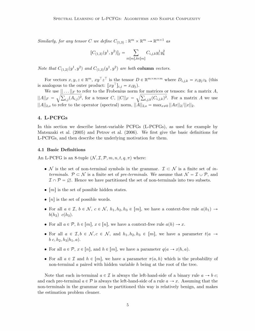
Similarly, for any tensor C we define Cp1,3q : Rm ˆ Rm Ñ Rmˆ1 as
rCp1,3qpy1, y2qsj “
ÿ
iPrms,kPrms
Ci,j,ky1i y
2k
Note that Cp1,2qpy1, y2q and Cp1,3qpy
1, y2q are both column vectors.
For vectors x, y, z P Rm, xyJzJ is the tensor D P Rmˆmˆm where Di,j,k “ xiyjzk (thisis analogous to the outer product: rxyJsi,j “ xiyj).
We use || . . . ||F to refer to the Frobenius norm for matrices or tensors: for a matrix A,
||A||F “b
ř
i,jpAi,jq2, for a tensor C, ||C||F “
b
ř
i,j,kpCi,j,kq2. For a matrix A we use
||A||2,o to refer to the operator (spectral) norm, ||A||2,o “ maxx‰0 ||Ax||2||x||2.
4. L-PCFGs
In this section we describe latent-variable PCFGs (L-PCFGs), as used for example byMatsuzaki et al. (2005) and Petrov et al. (2006). We first give the basic definitions forL-PCFGs, and then describe the underlying motivation for them.
4.1 Basic Definitions
An L-PCFG is an 8-tuple pN , I,P,m, n, t, q, πq where:
• N is the set of non-terminal symbols in the grammar. I Ă N is a finite set of in-terminals. P Ă N is a finite set of pre-terminals. We assume that N “ I Y P, andI X P “ H. Hence we have partitioned the set of non-terminals into two subsets.
• rms is the set of possible hidden states.
• rns is the set of possible words.
• For all a P I, b P N , c P N , h1, h2, h3 P rms, we have a context-free rule aph1q Ñ
bph2q cph3q.
• For all a P P, h P rms, x P rns, we have a context-free rule aphq Ñ x.
• For all a P I, b P N , c P N , and h1, h2, h3 P rms, we have a parameter tpa Ñb c, h2, h3|h1, aq.
• For all a P P, x P rns, and h P rms, we have a parameter qpaÑ x|h, aq.
• For all a P I and h P rms, we have a parameter πpa, hq which is the probability ofnon-terminal a paired with hidden variable h being at the root of the tree.
Note that each in-terminal a P I is always the left-hand-side of a binary rule a Ñ b c;and each pre-terminal a P P is always the left-hand-side of a rule aÑ x. Assuming that thenon-terminals in the grammar can be partitioned this way is relatively benign, and makesthe estimation problem cleaner.
5
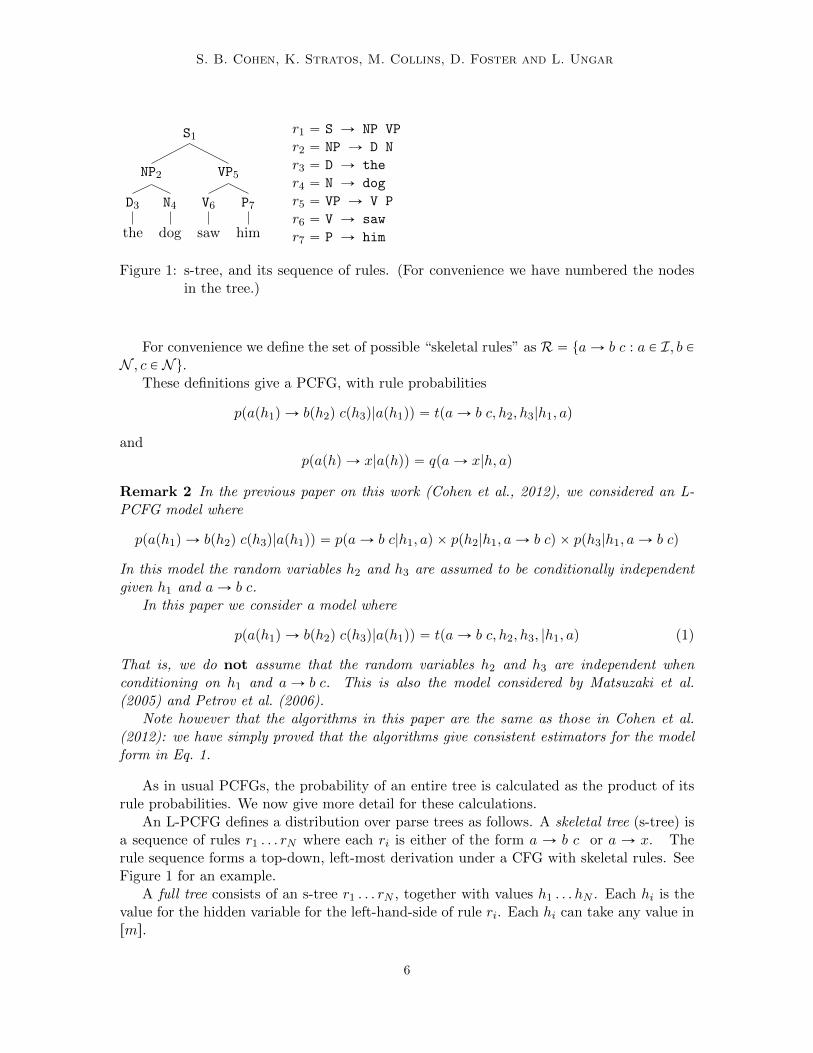
S. B. Cohen, K. Stratos, M. Collins, D. Foster and L. Ungar
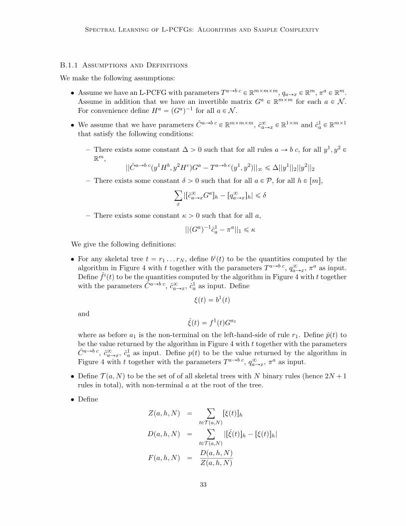
S1
NP2
D3
the
N4
dog
VP5
V6
saw
P7
him
r1 “ S Ñ NP VP
r2 “ NP Ñ D N
r3 “ D Ñ the
r4 “ N Ñ dog
r5 “ VP Ñ V P
r6 “ V Ñ saw
r7 “ P Ñ him
Figure 1: s-tree, and its sequence of rules. (For convenience we have numbered the nodesin the tree.)
For convenience we define the set of possible “skeletal rules” as R “ taÑ b c : a P I, b PN , c P N u.
These definitions give a PCFG, with rule probabilities
ppaph1q Ñ bph2q cph3q|aph1qq “ tpaÑ b c, h2, h3|h1, aq
andppaphq Ñ x|aphqq “ qpaÑ x|h, aq
Remark 2 In the previous paper on this work (Cohen et al., 2012), we considered an L-PCFG model where
ppaph1q Ñ bph2q cph3q|aph1qq “ ppaÑ b c|h1, aq ˆ pph2|h1, aÑ b cq ˆ pph3|h1, aÑ b cq
In this model the random variables h2 and h3 are assumed to be conditionally independentgiven h1 and aÑ b c.
In this paper we consider a model where
ppaph1q Ñ bph2q cph3q|aph1qq “ tpaÑ b c, h2, h3, |h1, aq (1)
That is, we do not assume that the random variables h2 and h3 are independent whenconditioning on h1 and aÑ b c. This is also the model considered by Matsuzaki et al.(2005) and Petrov et al. (2006).
Note however that the algorithms in this paper are the same as those in Cohen et al.(2012): we have simply proved that the algorithms give consistent estimators for the modelform in Eq. 1.
As in usual PCFGs, the probability of an entire tree is calculated as the product of itsrule probabilities. We now give more detail for these calculations.
An L-PCFG defines a distribution over parse trees as follows. A skeletal tree (s-tree) isa sequence of rules r1 . . . rN where each ri is either of the form a Ñ b c or a Ñ x. Therule sequence forms a top-down, left-most derivation under a CFG with skeletal rules. SeeFigure 1 for an example.
A full tree consists of an s-tree r1 . . . rN , together with values h1 . . . hN . Each hi is thevalue for the hidden variable for the left-hand-side of rule ri. Each hi can take any value inrms.
6
Spectral Learning of L-PCFGs: Algorithms and Sample Complexity
Define ai to be the non-terminal on the left-hand-side of rule ri. For any i P rN s such
that ai P I (i.e., ai is an in-terminal, and rule ri is of the form aÑ b c) define hp2qi to be the
hidden variable value associated with the left child of the rule ri, and hp3qi to be the hidden
variable value associated with the right child. The probability mass function (PMF) overfull trees is then
ppr1 . . . rN , h1 . . . hN q “ πpa1, h1q ˆź
i:aiPItpri, h
p2qi , h
p3qi |hi, aiq ˆ
ź
i:aiPPqpri|hi, aiq (2)
The PMF over s-trees is ppr1 . . . rN q “ř
h1...hNppr1 . . . rN , h1 . . . hN q.
In the remainder of this paper, we make use of a matrix form of parameters of anL-PCFG, as follows:
• For each aÑ b c P R, we define T aÑb c P Rmˆmˆm to be the tensor with values
T aÑb ch1,h2,h3 “ tpaÑ b c, h2, h3|a, h1q
• For each a P P, x P rns, we define qaÑx P R1ˆm to be the row vector with values
rqaÑxsh “ qpaÑ x|h, aq
for h “ 1, 2, . . .m.
‚ For each a P I, we define the column vector πa P Rmˆ1 where rπash “ πpa, hq.
4.2 Application of L-PCFGs to Natural Language Parsing
L-PCFGs have been shown to be a very useful model for natural language parsing (Mat-suzaki et al., 2005; Petrov et al., 2006). In this section we describe the basic approach.
We assume a training set consisting of sentences paired with parse trees, which aresimilar to the skeletal tree shown in Figure 1. A naive approach to parsing would simplyread off a PCFG from the training set: the resulting grammar would have rules such as
S Ñ NP VP
NP Ñ D N
VP Ñ V NP
D Ñ the
N Ñ dog
and so on. Given a test sentence, the most likely parse under the PCFG can be found usingdynamic programming algorithms.
Unfortunately, simple “vanilla” PCFGs induced from treebanks such as the Penn tree-bank (Marcus et al., 1993) typically give very poor parsing performance. A critical issueis that the set of non-terminals in the resulting grammar (S, NP, VP, PP, D, N, etc.) isoften quite small. The resulting PCFG therefore makes very strong independence assump-tions, failing to capture important statistical properties of parse trees.
In response to this issue, a number of PCFG-based models have been developed whichmake use of grammars with refined non-terminals. For example, in lexicalized models
7
S. B. Cohen, K. Stratos, M. Collins, D. Foster and L. Ungar
(Collins, 1997; Charniak, 1997), non-terminals such as S are replaced with non-terminalssuch as S-sleeps: the non-terminals track some lexical item (in this case sleeps), in additionto the syntactic category. For example, the parse tree in Figure 1 would include rules
S-saw Ñ NP-dog VP-saw
NP-dog Ñ D-the N-dog
VP-saw Ñ V-saw P-him
D-the Ñ the
N-dog Ñ dog
V-saw Ñ saw
P-him Ñ him
In this case the number of non-terminals in the grammar increases dramatically, butwith appropriate smoothing of parameter estimates lexicalized models perform at muchhigher accuracy than vanilla PCFGs.
As another example, Johnson (1998) describes an approach where non-terminals arerefined to also include the non-terminal one level up in the tree; for example rules such as
S Ñ NP VP
are replaced by rules such as
S-ROOT Ñ NP-S VP-S
Here NP-S corresponds to an NP non-terminal whose parent is S; VP-S corresponds to a VP
whose parent is S; S-ROOT corresponds to an S which is at the root of the tree. This simplemodification leads to significant improvements over a vanilla PCFG.
Klein and Manning (2003) develop this approach further, introducing annotations cor-responding to parents and siblings in the tree, together with other information, resultingin a parser whose performance is just below the lexicalized models of Collins (1997) andCharniak (1997).
The approaches of Collins (1997), Charniak (1997), Johnson (1998), and Klein andManning (2003) all use hand-constructed rules to enrich the set of non-terminals in thePCFG. A natural question is whether refinements to non-terminals can be learned auto-matically. Matsuzaki et al. (2005) and Petrov et al. (2006) addressed this question throughthe use of L-PCFGs in conjunction with the EM algorithm. The basic idea is to allow eachnon-terminal in the grammar to have m possible latent values. For example, with m “ 8we would replace the non-terminal S with non-terminals S-1, S-2, . . ., S-8, and we wouldreplace rules such as
S Ñ NP VP
with rules such as
S-4 Ñ NP-3 VP-2
The latent values are of course unobserved in the training data (the treebank), but they canbe treated as latent variables in a PCFG-based model, and the parameters of the model can
8
Spectral Learning of L-PCFGs: Algorithms and Sample Complexity
be estimated using the EM algorithm. More specifically, given training examples consisting
of skeletal trees of the form tpiq “ prpiq1 , r
piq2 , . . . , r
piqNiq, for i “ 1 . . .M , where Ni is the number
of rules in the i’th tree, the log-likelihood of the training data is
Mÿ
i“1
log pprpiq1 . . . r
piqNiq “
Mÿ
i“1
logÿ
h1...hNi
pprpiq1 . . . r
piqNi, h1 . . . hNiq
where pprpiq1 . . . r
piqNi, h1 . . . hNiq is as defined in Eq. 2. The EM algorithm is guaranteed to
converge to a local maximum of the log-likelihood function. Once the parameters of theL-PCFG have been estimated, the algorithm of Goodman (1996) can be used to parse test-data sentences using the L-PCFG: see Section 4.3 for more details. Matsuzaki et al. (2005)and Petrov et al. (2006) show very good performance for these methods.
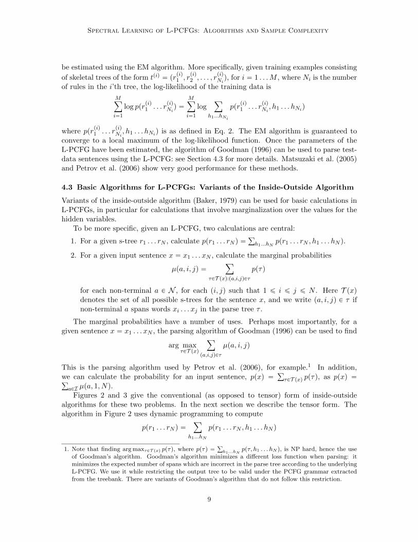
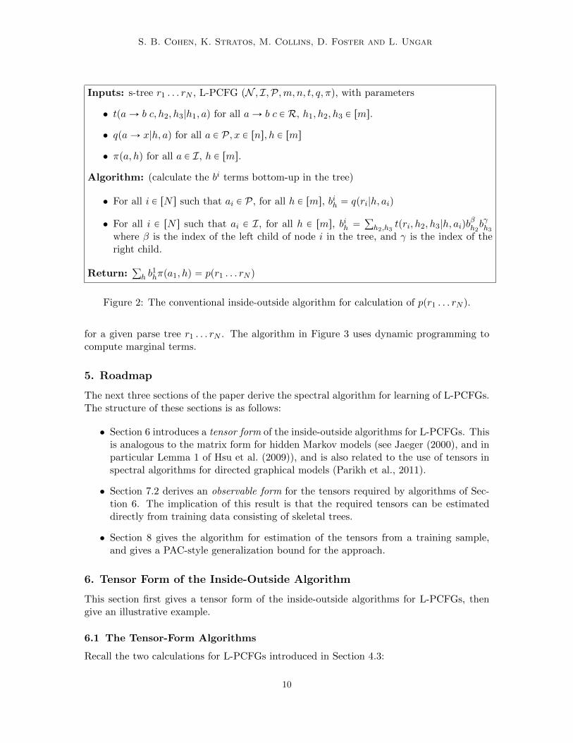
4.3 Basic Algorithms for L-PCFGs: Variants of the Inside-Outside Algorithm
Variants of the inside-outside algorithm (Baker, 1979) can be used for basic calculations inL-PCFGs, in particular for calculations that involve marginalization over the values for thehidden variables.
To be more specific, given an L-PCFG, two calculations are central:
1. For a given s-tree r1 . . . rN , calculate ppr1 . . . rN q “ř
h1...hNppr1 . . . rN , h1 . . . hN q.
2. For a given input sentence x “ x1 . . . xN , calculate the marginal probabilities
µpa, i, jq “ÿ
τPT pxq:pa,i,jqPτppτq
for each non-terminal a P N , for each pi, jq such that 1 ď i ď j ď N . Here T pxqdenotes the set of all possible s-trees for the sentence x, and we write pa, i, jq P τ ifnon-terminal a spans words xi . . . xj in the parse tree τ .
The marginal probabilities have a number of uses. Perhaps most importantly, for agiven sentence x “ x1 . . . xN , the parsing algorithm of Goodman (1996) can be used to find
arg maxτPT pxq
ÿ
pa,i,jqPτ
µpa, i, jq
This is the parsing algorithm used by Petrov et al. (2006), for example.1 In addition,we can calculate the probability for an input sentence, ppxq “
ř
τPT pxq ppτq, as ppxq “ř
aPI µpa, 1, Nq.Figures 2 and 3 give the conventional (as opposed to tensor) form of inside-outside
algorithms for these two problems. In the next section we describe the tensor form. Thealgorithm in Figure 2 uses dynamic programming to compute
ppr1 . . . rN q “ÿ
h1...hN
ppr1 . . . rN , h1 . . . hN q
1. Note that finding arg maxτPT pxq ppτq, where ppτq “ř
h1...hNppτ, h1 . . . hN q, is NP hard, hence the use
of Goodman’s algorithm. Goodman’s algorithm minimizes a different loss function when parsing: itminimizes the expected number of spans which are incorrect in the parse tree according to the underlyingL-PCFG. We use it while restricting the output tree to be valid under the PCFG grammar extractedfrom the treebank. There are variants of Goodman’s algorithm that do not follow this restriction.
9
S. B. Cohen, K. Stratos, M. Collins, D. Foster and L. Ungar
Inputs: s-tree r1 . . . rN , L-PCFG pN , I,P,m, n, t, q, πq, with parameters
• tpaÑ b c, h2, h3|h1, aq for all aÑ b c P R, h1, h2, h3 P rms.
• qpaÑ x|h, aq for all a P P, x P rns, h P rms
• πpa, hq for all a P I, h P rms.
Algorithm: (calculate the bi terms bottom-up in the tree)
• For all i P rN s such that ai P P, for all h P rms, bih “ qpri|h, aiq
• For all i P rN s such that ai P I, for all h P rms, bih “ř
h2,h3tpri, h2, h3|h, aiqb
βh2bγh3
where β is the index of the left child of node i in the tree, and γ is the index of theright child.
Return:ř
h b1hπpa1, hq “ ppr1 . . . rN q
Figure 2: The conventional inside-outside algorithm for calculation of ppr1 . . . rN q.
for a given parse tree r1 . . . rN . The algorithm in Figure 3 uses dynamic programming tocompute marginal terms.
5. Roadmap
The next three sections of the paper derive the spectral algorithm for learning of L-PCFGs.The structure of these sections is as follows:
• Section 6 introduces a tensor form of the inside-outside algorithms for L-PCFGs. Thisis analogous to the matrix form for hidden Markov models (see Jaeger (2000), and inparticular Lemma 1 of Hsu et al. (2009)), and is also related to the use of tensors inspectral algorithms for directed graphical models (Parikh et al., 2011).
• Section 7.2 derives an observable form for the tensors required by algorithms of Sec-tion 6. The implication of this result is that the required tensors can be estimateddirectly from training data consisting of skeletal trees.
• Section 8 gives the algorithm for estimation of the tensors from a training sample,and gives a PAC-style generalization bound for the approach.
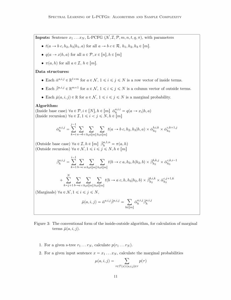
6. Tensor Form of the Inside-Outside Algorithm
This section first gives a tensor form of the inside-outside algorithms for L-PCFGs, thengive an illustrative example.
6.1 The Tensor-Form Algorithms
Recall the two calculations for L-PCFGs introduced in Section 4.3:
10
Spectral Learning of L-PCFGs: Algorithms and Sample Complexity
Inputs: Sentence x1 . . . xN , L-PCFG pN , I,P,m, n, t, q, πq, with parameters
• tpaÑ b c, h2, h3|h1, aq for all aÑ b c P R, h1, h2, h3 P rms.
• qpaÑ x|h, aq for all a P P, x P rns, h P rms
• πpa, hq for all a P I, h P rms.
Data structures:
• Each αa,i,j P R1ˆm for a P N , 1 ď i ď j ď N is a row vector of inside terms.
• Each βa,i,j P Rmˆ1 for a P N , 1 ď i ď j ď N is a column vector of outside terms.
• Each µpa, i, jq P R for a P N , 1 ď i ď j ď N is a marginal probability.
Algorithm:(Inside base case) @a P P, i P rN s, h P rms αa,i,ih “ qpaÑ xi|h, aq(Inside recursion) @a P I, 1 ď i ă j ď N,h P rms
αa,i,jh “
j´1ÿ
k“i
ÿ
aÑb c
ÿ
h2Prms
ÿ
h3Prms
tpaÑ b c, h2, h3|h, aq ˆ αb,i,kh2
ˆ αc,k`1,jh3
(Outside base case) @a P I, h P rms βa,1,nh “ πpa, hq(Outside recursion) @a P N , 1 ď i ď j ď N,h P rms
βa,i,jh “
i´1ÿ
k“1
ÿ
bÑc a
ÿ
h2Prms
ÿ
h3Prms
tpbÑ c a, h3, h|h2, bq ˆ βb,k,jh2
ˆ αc,k,i´1h3
`
Nÿ
k“j`1
ÿ
bÑa c
ÿ
h2Prms
ÿ
h3Prms
tpbÑ a c, h, h3|h2, bq ˆ βb,i,kh2
ˆ αc,j`1,kh3
(Marginals) @a P N , 1 ď i ď j ď N,
µpa, i, jq “ αa,i,j βa,i,j “ÿ
hPrms
αa,i,jh βa,i,jh
Figure 3: The conventional form of the inside-outside algorithm, for calculation of marginalterms µpa, i, jq.
1. For a given s-tree r1 . . . rN , calculate ppr1 . . . rN q.
2. For a given input sentence x “ x1 . . . xN , calculate the marginal probabilities
µpa, i, jq “ÿ
τPT pxq:pa,i,jqPτppτq
11
S. B. Cohen, K. Stratos, M. Collins, D. Foster and L. Ungar
Inputs: s-tree r1 . . . rN , L-PCFG pN , I,P,m, nq, parameters
• CaÑb c P Rpmˆmˆmq for all aÑ b c P R
• c8aÑx P Rp1ˆmq for all a P P, x P rns
• c1a P Rpmˆ1q for all a P I.
Algorithm: (calculate the f i terms bottom-up in the tree)
• For all i P rN s such that ai P P, f i “ c8ri
• For all i P rN s such that ai P I, f i “ Cripfβ, fγq where β is the index of the left childof node i in the tree, and γ is the index of the right child.
Return: f1c1a1 “ ppr1 . . . rN q
Figure 4: The tensor form for calculation of ppr1 . . . rN q.
for each non-terminal a P N , for each pi, jq such that 1 ď i ď j ď N , where T pxqdenotes the set of all possible s-trees for the sentence x, and we write pa, i, jq P τ ifnon-terminal a spans words xi . . . xj in the parse tree τ .
The tensor form of the inside-outside algorithms for these two problems are shown inFigures 4 and 5. Each algorithm takes the following inputs:
1. A tensor CaÑb c P Rpmˆmˆmq for each rule aÑ b c.
2. A vector c8aÑx P Rp1ˆmq for each rule aÑ x.
3. A vector c1a P Rpmˆ1q for each a P I.
The following theorem gives conditions under which the algorithms are correct:
Theorem 3 Assume that we have an L-PCFG with parameters qaÑx, T aÑb c, πa, and thatthere exist matrices Ga P Rpmˆmq for all a P N such that each Ga is invertible, and suchthat:
1. For all rules aÑ b c, CaÑb cpy1, y2q “`
T aÑb cpy1Gb, y2Gcq˘
pGaq´1
2. For all rules aÑ x, c8aÑx “ qaÑxpGaq´1
3. For all a P I, c1a “ Gaπa
Then: 1) The algorithm in Figure 4 correctly computes ppr1 . . . rN q under the L-PCFG. 2)The algorithm in Figure 5 correctly computes the marginals µpa, i, jq under the L-PCFG.
Proof: see Section A.1. The next section (Section 6.2) gives an example that illustratesthe basic intuition behind the proof.
12
Spectral Learning of L-PCFGs: Algorithms and Sample Complexity
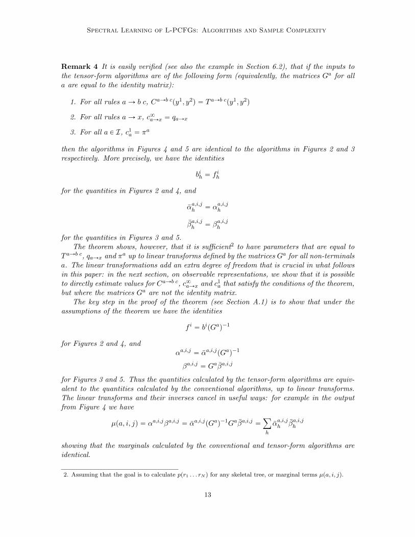
Remark 4 It is easily verified (see also the example in Section 6.2), that if the inputs tothe tensor-form algorithms are of the following form (equivalently, the matrices Ga for alla are equal to the identity matrix):
1. For all rules aÑ b c, CaÑb cpy1, y2q “ T aÑb cpy1, y2q
2. For all rules aÑ x, c8aÑx “ qaÑx
3. For all a P I, c1a “ πa
then the algorithms in Figures 4 and 5 are identical to the algorithms in Figures 2 and 3respectively. More precisely, we have the identities
bih “ f ih
for the quantities in Figures 2 and 4, and
αa,i,jh “ αa,i,jh
βa,i,jh “ βa,i,jh
for the quantities in Figures 3 and 5.The theorem shows, however, that it is sufficient2 to have parameters that are equal to
T aÑb c, qaÑx and πa up to linear transforms defined by the matrices Ga for all non-terminalsa. The linear transformations add an extra degree of freedom that is crucial in what followsin this paper: in the next section, on observable representations, we show that it is possibleto directly estimate values for CaÑb c, c8aÑx and c1
a that satisfy the conditions of the theorem,but where the matrices Ga are not the identity matrix.
The key step in the proof of the theorem (see Section A.1) is to show that under theassumptions of the theorem we have the identities
f i “ bipGaq´1
for Figures 2 and 4, andαa,i,j “ αa,i,jpGaq´1
βa,i,j “ Gaβa,i,j
for Figures 3 and 5. Thus the quantities calculated by the tensor-form algorithms are equiv-alent to the quantities calculated by the conventional algorithms, up to linear transforms.The linear transforms and their inverses cancel in useful ways: for example in the outputfrom Figure 4 we have
µpa, i, jq “ αa,i,jβa,i,j “ αa,i,jpGaq´1Gaβa,i,j “ÿ
h
αa,i,jh βa,i,jh
showing that the marginals calculated by the conventional and tensor-form algorithms areidentical.
2. Assuming that the goal is to calculate ppr1 . . . rN q for any skeletal tree, or marginal terms µpa, i, jq.
13
S. B. Cohen, K. Stratos, M. Collins, D. Foster and L. Ungar
Inputs: Sentence x1 . . . xN , L-PCFG pN , I,P,m, nq, parameters CaÑb c P Rpmˆmˆmq forall aÑ b c P R, c8aÑx P Rp1ˆmq for all a P P, x P rns, c1
a P Rpmˆ1q for all a P I.Data structures:
• Each αa,i,j P R1ˆm for a P N , 1 ď i ď j ď N is a row vector of inside terms.
• Each βa,i,j P Rmˆ1 for a P N , 1 ď i ď j ď N is a column vector of outside terms.
• Each µpa, i, jq P R for a P N , 1 ď i ď j ď N is a marginal probability.
Algorithm:(Inside base case) @a P P, i P rN s, αa,i,i “ c8aÑxi(Inside recursion) @a P I, 1 ď i ă j ď N,
αa,i,j “
j´1ÿ
k“i
ÿ
aÑb c
CaÑb cpαb,i,k, αc,k`1,jq
(Outside base case) @a P I, βa,1,n “ c1a
(Outside recursion) @a P N , 1 ď i ď j ď N,
βa,i,j “i´1ÿ
k“1
ÿ
bÑc a
CbÑc ap1,2q pβb,k,j , αc,k,i´1q
`
Nÿ
k“j`1
ÿ
bÑa c
CbÑa cp1,3q pβb,i,k, αc,j`1,kq
(Marginals) @a P N , 1 ď i ď j ď N,
µpa, i, jq “ αa,i,jβa,i,j “ÿ
hPrms
αa,i,jh βa,i,jh
Figure 5: The tensor form of the inside-outside algorithm, for calculation of marginal termsµpa, i, jq.
6.2 An Example
In the remainder of this section we give an example that illustrates how the algorithm inFigure 4 is correct, and gives the basic intuition behind the proof in Section A.1. While weconcentrate on the algorithm in Figure 4, the intuition behind the algorithm in Figure 5 isvery similar.
Consider the skeletal tree in Figure 6. We will demonstrate how the algorithm inFigure 4, under the assumptions in the theorem, correctly calculates the probability ofthis tree. In brief, the argument involves the following steps:
14
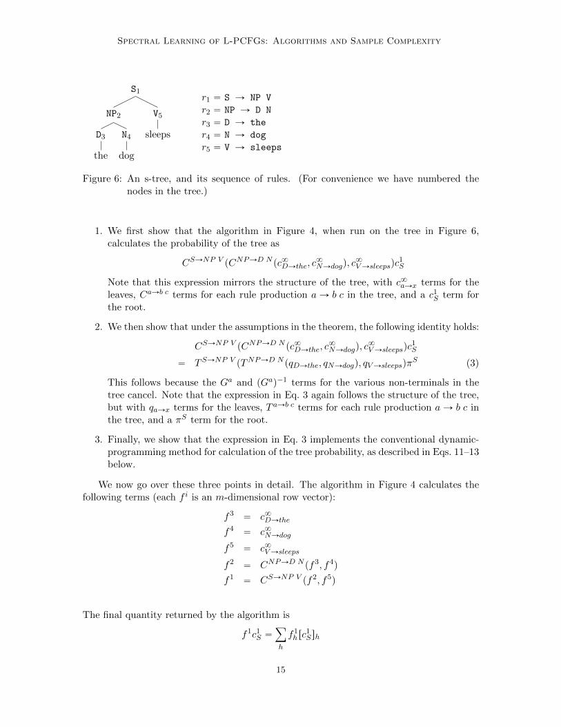
Spectral Learning of L-PCFGs: Algorithms and Sample Complexity
S1
NP2
D3
the
N4
dog
V5
sleeps
r1 “ S Ñ NP V
r2 “ NP Ñ D N
r3 “ D Ñ the
r4 “ N Ñ dog
r5 “ V Ñ sleeps
Figure 6: An s-tree, and its sequence of rules. (For convenience we have numbered thenodes in the tree.)
1. We first show that the algorithm in Figure 4, when run on the tree in Figure 6,calculates the probability of the tree as
CSÑNP V pCNPÑD N pc8DÑthe, c8NÑdogq, c
8VÑsleepsqc
1S
Note that this expression mirrors the structure of the tree, with c8aÑx terms for theleaves, CaÑb c terms for each rule production aÑ b c in the tree, and a c1
S term forthe root.
2. We then show that under the assumptions in the theorem, the following identity holds:
CSÑNP V pCNPÑD N pc8DÑthe, c8NÑdogq, c
8VÑsleepsqc
1S
“ TSÑNP V pTNPÑD N pqDÑthe, qNÑdogq, qVÑsleepsqπS (3)
This follows because the Ga and pGaq´1 terms for the various non-terminals in thetree cancel. Note that the expression in Eq. 3 again follows the structure of the tree,but with qaÑx terms for the leaves, T aÑb c terms for each rule production aÑ b c inthe tree, and a πS term for the root.
3. Finally, we show that the expression in Eq. 3 implements the conventional dynamic-programming method for calculation of the tree probability, as described in Eqs. 11–13below.
We now go over these three points in detail. The algorithm in Figure 4 calculates thefollowing terms (each f i is an m-dimensional row vector):
f3 “ c8DÑthe
f4 “ c8NÑdog
f5 “ c8VÑsleeps
f2 “ CNPÑD N pf3, f4q
f1 “ CSÑNP V pf2, f5q
The final quantity returned by the algorithm is
f1c1S “
ÿ
h
f1hrc
1Ssh
15
S. B. Cohen, K. Stratos, M. Collins, D. Foster and L. Ungar
Combining the definitions above, it can be seen that
f1c1S “ CSÑNP V pCNPÑD N pc8DÑthe, c
8NÑdogq, c
8VÑsleepsqc
1S
demonstrating that point 1 above holds.Next, given the assumptions in the theorem, we show point 2, that is, that
CSÑNP V pCNPÑD N pc8DÑthe, c8NÑdogq, c
8VÑsleepsqc
1S
“ TSÑNP V pTNPÑD N pqDÑthe, qNÑdogq, qVÑsleepsqπS (4)
This follows because the Ga and pGaq´1 terms in the theorem cancel. More specifically, wehave
f3 “ c8DÑthe “ qDÑthepGDq´1 (5)
f4 “ c8NÑdog “ qNÑdogpGN q´1 (6)
f5 “ c8VÑsleeps “ qVÑsleepspGV q´1 (7)
f2 “ CNPÑD N pf3, f4q “ TNPÑD N pqDÑthe, qDÑdogqpGNP q´1 (8)
f1 “ CSÑNP V pf2, f5q “ TSÑNP V pTNPÑD N pqDÑthe, qNÑdogq, qVÑsleepsqpGSq´1 (9)
Eqs. 5, 6, 7 follow by the assumptions in the theorem. Eq. 8 follows because by the assump-tions in the theorem
CNPÑD N pf3, f4q “ TNPÑD N pf3GD, f4GN qpGNP q´1
hence
CNPÑD N pf3, f4q “ TNPÑD N pqDÑthepGDq´1GD, qNÑdogpG
N q´1GN qpGNP q´1
“ TNPÑD N pqDÑthe, qNÑdogqpGNP q´1
Eq. 9 follows in a similar manner.It follows by the assumption that c1
S “ GSπS that
CSÑNP V pCNPÑD N pc8DÑthe, c8NÑdogq, c
8VÑsleepsqc
1S
“ TSÑNP V pTNPÑD N pqDÑthe, qNÑdogq, qVÑsleepsqpGSq´1GSπS
“ TSÑNP V pTNPÑD N pqDÑthe, qNÑdogq, qVÑsleepsqπS (10)
The final step (point 3) is to show that the expression in Eq. 10 correctly calculates theprobability of the example tree. First consider the term TNPÑD N pqDÑthe, qNÑdogq—thisis an m-dimensional row vector, call this b2. By the definition of the tensor TNPÑD N , wehave
b2h ““
TNPÑD N pqDÑthe, qNÑdogq‰
h
“ÿ
h2,h3
tpNP Ñ D N,h2, h3|h,NP q ˆ qpD Ñ the|h2, Dq ˆ qpN Ñ dog|h3, Nq(11)
16
Spectral Learning of L-PCFGs: Algorithms and Sample Complexity
By a similar calculation, TSÑNP V pTNPÑD N pqDÑthe, qNÑdogq, qVÑsleepsq—call this vectorb1—is
b1h “ÿ
h2,h3
tpS Ñ NP V, h2, h3|h, Sq ˆ b2h2 ˆ qpV Ñ sleeps|h3, V q (12)
Finally, the probability of the full tree is calculated as
ÿ
h
b1hπSh (13)
It can be seen that the expression in Eq. 4 implements the calculations in Eqs. 11, 12and 13, which are precisely the calculations used in the conventional dynamic programmingalgorithm for calculation of the probability of the tree.
7. Estimating the Tensor Model
A crucial result is that it is possible to directly estimate parameters CaÑb c, c8aÑx and c1a
that satisfy the conditions in Theorem 3, from a training sample consisting of s-trees (i.e.,trees where hidden variables are unobserved). We first describe random variables underlyingthe approach, then describe observable representations based on these random variables.
7.1 Random Variables Underlying the Approach
Each s-tree with N rules r1 . . . rN has N nodes. We will use the s-tree in Figure 1 as arunning example.
Each node has an associated rule: for example, node 2 in the tree in Figure 1 has therule NP Ñ D N. If the rule at a node is of the form aÑ b c, then there are left and rightinside trees below the left child and right child of the rule. For example, for node 2 we havea left inside tree rooted at node 3, and a right inside tree rooted at node 4 (in this case theleft and right inside trees both contain only a single rule production, of the form a Ñ x;however in the general case they might be arbitrary subtrees).
In addition, each node has an outside tree. For node 2, the outside tree isS
NP VP
V
saw
P
himThe outside tree contains everything in the s-tree r1 . . . rN , excluding the subtree belownode i.
Our random variables are defined as follows. First, we select a random internal node,from a random tree, as follows:
• Sample a full tree r1 . . . rN , h1 . . . hN from the PMF ppr1 . . . rN , h1 . . . hN q.
• Choose a node i uniformly at random from rN s.
If the rule ri for the node i is of the form aÑ b c, we define random variables as follows:
17
S. B. Cohen, K. Stratos, M. Collins, D. Foster and L. Ungar
• R1 is equal to the rule ri (e.g., NPÑ D N).
• T1 is the inside tree rooted at node i. T2 is the inside tree rooted at the left child ofnode i, and T3 is the inside tree rooted at the right child of node i.
• H1, H2, H3 are the hidden variables associated with node i, the left child of node i,and the right child of node i respectively.
• A1, A2, A3 are the labels for node i, the left child of node i, and the right child of nodei respectively. (E.g., A1 “ NP, A2 “ D, A3 “ N.)
• O is the outside tree at node i.
• B is equal to 1 if node i is at the root of the tree (i.e., i “ 1), 0 otherwise.
If the rule ri for the selected node i is of the form a Ñ x, we have random variablesR1, T1, H1, A1, O,B as defined above, but H2, H3, T2, T3, A2, and A3 are not defined.
We assume a function ψ that maps outside trees o to feature vectors ψpoq P Rd1
. Forexample, the feature vector might track the rule directly above the node in question, theword following the node in question, and so on. We also assume a function φ that mapsinside trees t to feature vectors φptq P Rd. As one example, the function φ might be anindicator function tracking the rule production at the root of the inside tree. Later we giveformal criteria for what makes good definitions of ψpoq and φptq. One requirement is thatd1 ě m and d ě m.
In tandem with these definitions, we assume projection matices Ua P Rpdˆmq and V a P
Rpd1ˆmq for all a P N . We then define additional random variables Y1, Y2, Y3, Z as
Y1 “ pUa1qJφpT1q Z “ pV
a1qJψpOq
Y2 “ pUa2qJφpT2q Y3 “ pU
a3qJφpT3q
where ai is the value of the random variable Ai. Note that Y1, Y2, Y3, Z are all in Rm.
7.2 Observable Representations
Given the definitions in the previous section, our representation is based on the followingmatrix, tensor and vector quantities, defined for all a P N , for all rules of the form aÑ b c,and for all rules of the form aÑ x respectively:
Σa “ ErY1ZJ|A1 “ as
DaÑb c “ E“
vR1 “ aÑ b cwZY J2 YJ
3 |A1 “ a‰
d8aÑx “ E“
vR1 “ aÑ xwZJ|A1 “ a‰
Assuming access to functions φ and ψ, and projection matrices Ua and V a, these quantitiescan be estimated directly from training data consisting of a set of s-trees (see Section 8).
Our observable representation then consists of:
CaÑb cpy1, y2q “ DaÑb cpy1, y2qpΣaq´1 (14)
c8aÑx “ d8aÑxpΣaq´1 (15)
c1a “ E rvA1 “ awY1|B “ 1s (16)
18
Spectral Learning of L-PCFGs: Algorithms and Sample Complexity
We next introduce conditions under which these quantities satisfy the conditions in Theo-rem 3.
The following definition will be important:
Definition 5 For all a P N , we define the matrices Ia P Rpdˆmq and Ja P Rpd1ˆmq as
rIasi,h “ ErφipT1q | H1 “ h,A1 “ as
rJasi,h “ ErψipOq | H1 “ h,A1 “ as
In addition, for any a P N , we use γa P Rm to denote the vector with γah “ P pH1 “ h|A1 “
aq.
The correctness of the representation will rely on the following conditions being satisfied(these are parallel to conditions 1 and 2 in Hsu et al. (2009)):
Condition 1 @a P N , the matrices Ia and Ja are of full rank (i.e., they have rank m).For all a P N , for all h P rms, γah ą 0.
Condition 2 @a P N , the matrices Ua P Rpdˆmq and V a P Rpd1ˆmq are such that the
matrices Ga “ pUaqJIa and Ka “ pV aqJJa are invertible.
We can now state the following theorem:
Theorem 6 Assume conditions 1 and 2 are satisfied. For all a P N , define Ga “ pUaqJIa.Then under the definitions in Eqs. 14-16:
1. For all rules aÑ b c, CaÑb cpy1, y2q “`
T aÑb cpy1Gb, y2Gcq˘
pGaq´1
2. For all rules aÑ x, c8aÑx “ qaÑxpGaq´1.
3. For all a P N , c1a “ Gaπa
Proof: The following identities hold (see Section A.2):
DaÑb cpy1, y2q “
´
T aÑb cpy1Gb, y2Gcq¯
diagpγaqpKaqJ (17)
d8aÑx “ qaÑxdiagpγaqpKaqJ (18)
Σa “ GadiagpγaqpKaqJ (19)
c1a “ Gaπa (20)
Under conditions 1 and 2, Σa is invertible, and pΣaq´1 “ ppKaqJq´1pdiagpγaqq´1pGaq´1.The identities in the theorem follow immediately.
This theorem leads directly to the spectral learning algorithm, which we describe in thenext section. We give a sketch of the approach here. Assume that we have a training setconsisting of skeletal trees (no latent variables are observed) generated from some under-lying L-PCFG. Assume in addition that we have definitions of φ, ψ, Ua and V a such that
19
S. B. Cohen, K. Stratos, M. Collins, D. Foster and L. Ungar
conditions 1 and 2 are satisfied for the L-PCFG. Then it is straightforward to use the train-ing examples to derive i.i.d. samples from the joint distribution over the random variablespA1, R1, Y1, Y2, Y3, Z,Bq used in the definitions in Eqs. 14–16. These samples can be usedto estimate the quantities in Eqs. 14–16; the estimated quantities CaÑb c, c8aÑx and c1
a canthen be used as inputs to the algorithms in Figures 4 and 5. By standard arguments, theestimates CaÑb c, c8aÑx and c1
a will converge to the values in Eqs. 14–16.The following lemma justifies the use of an SVD calculation as one method for finding
values for Ua and V a that satisfy condition 2, assuming that condition 1 holds:
Lemma 7 Assume that condition 1 holds, and for all a P N define
Ωa “ ErφpT1q pψpOqqJ|A1 “ as (21)
Then if Ua is a matrix of the m left singular vectors of Ωa corresponding to non-zero singularvalues, and V a is a matrix of the m right singular vectors of Ωa corresponding to non-zerosingular values, then condition 2 is satisfied.
Proof sketch: It can be shown that Ωa “ IadiagpγaqpJaqJ. The remainder is similar tothe proof of lemma 2 in Hsu et al. (2009).
The matrices Ωa can be estimated directly from a training set consisting of s-trees,assuming that we have access to the functions φ and ψ. Similar arguments to those of Hsuet al. (2009) can be used to show that with a sufficient number of samples, the resultingestimates of Ua and V a satisfy condition 2 with high probability.
8. Deriving Empirical Estimates
Figure 7 shows an algorithm that derives estimates of the quantities in Eqs 14, 15, and16. As input, the algorithm takes a sequence of tuples prpi,1q, tpi,1q, tpi,2q, tpi,3q, opiq, bpiqq fori P rM s.
These tuples can be derived from a training set consisting of s-trees τ1 . . . τM as follows:‚ @i P rM s, choose a single node ji uniformly at random from the nodes in τi. Define
rpi,1q to be the rule at node ji. tpi,1q is the inside tree rooted at node ji. If rpi,1q is of the form
aÑ b c, then tpi,2q is the inside tree under the left child of node ji, and tpi,3q is the insidetree under the right child of node ji. If rpi,1q is of the form aÑ x, then tpi,2q “ tpi,3q “ NULL.opiq is the outside tree at node ji. b
piq is 1 if node ji is at the root of the tree, 0 otherwise.Under this process, assuming that the s-trees τ1 . . . τM are i.i.d. draws from the distribu-
tion ppτq over s-trees under an L-PCFG, the tuples prpi,1q, tpi,1q, tpi,2q, tpi,3q, opiq, bpiqq are i.i.d.draws from the joint distribution over the random variables R1, T1, T2, T3, O,B defined inthe previous section.
The algorithm first computes estimates of the projection matrices Ua and V a: followingLemma 7, this is done by first deriving estimates of Ωa, and then taking SVDs of each Ωa.The matrices are then used to project inside and outside trees tpi,1q, tpi,2q, tpi,3q, opiq down tom-dimensional vectors ypi,1q, ypi,2q, ypi,3q, zpiq; these vectors are used to derive the estimatesof CaÑb c, c8aÑx, and c1
a. For example, the quantities
DaÑb c “ E“
vR1 “ aÑ b cwZY J2 YJ
3 |A1 “ a‰
d8aÑx “ E“
vR1 “ aÑ xwZJ|A1 “ a‰
20
Spectral Learning of L-PCFGs: Algorithms and Sample Complexity
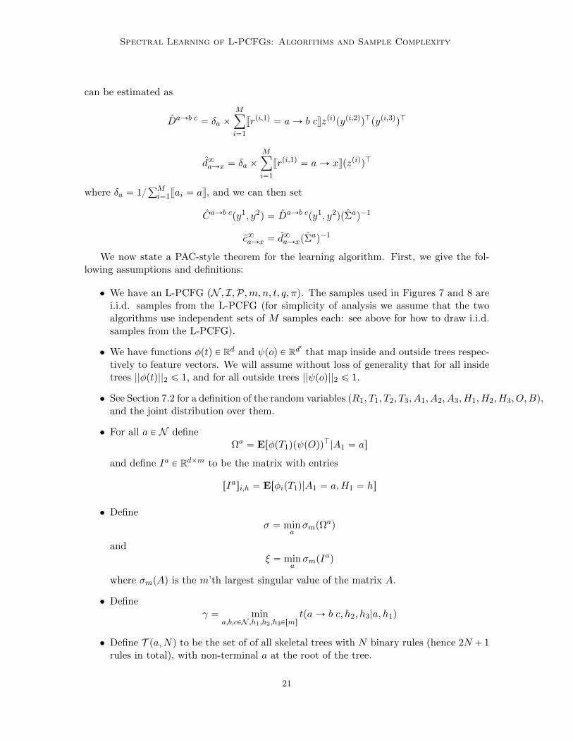
can be estimated as
DaÑb c “ δa ˆMÿ
i“1
vrpi,1q “ aÑ b cwzpiqpypi,2qqJpypi,3qqJ
d8aÑx “ δa ˆMÿ
i“1
vrpi,1q “ aÑ xwpzpiqqJ
where δa “ 1řMi“1vai “ aw, and we can then set
CaÑb cpy1, y2q “ DaÑb cpy1, y2qpΣaq´1
c8aÑx “ d8aÑxpΣaq´1
We now state a PAC-style theorem for the learning algorithm. First, we give the fol-lowing assumptions and definitions:
• We have an L-PCFG pN , I,P,m, n, t, q, πq. The samples used in Figures 7 and 8 arei.i.d. samples from the L-PCFG (for simplicity of analysis we assume that the twoalgorithms use independent sets of M samples each: see above for how to draw i.i.d.samples from the L-PCFG).
• We have functions φptq P Rd and ψpoq P Rd1
that map inside and outside trees respec-tively to feature vectors. We will assume without loss of generality that for all insidetrees ||φptq||2 ď 1, and for all outside trees ||ψpoq||2 ď 1.
• See Section 7.2 for a definition of the random variables pR1, T1, T2, T3, A1, A2, A3, H1, H2, H3, O,Bq,and the joint distribution over them.
• For all a P N defineΩa “ ErφpT1qpψpOqq
J|A1 “ as
and define Ia P Rdˆm to be the matrix with entries
rIasi,h “ ErφipT1q|A1 “ a,H1 “ hs
• Defineσ “ min
aσmpΩ
aq
andξ “ min
aσmpI
aq
where σmpAq is the m’th largest singular value of the matrix A.
• Defineγ “ min
a,b,cPN ,h1,h2,h3PrmstpaÑ b c, h2, h3|a, h1q
• Define T pa,Nq to be the set of of all skeletal trees with N binary rules (hence 2N ` 1rules in total), with non-terminal a at the root of the tree.
21
S. B. Cohen, K. Stratos, M. Collins, D. Foster and L. Ungar
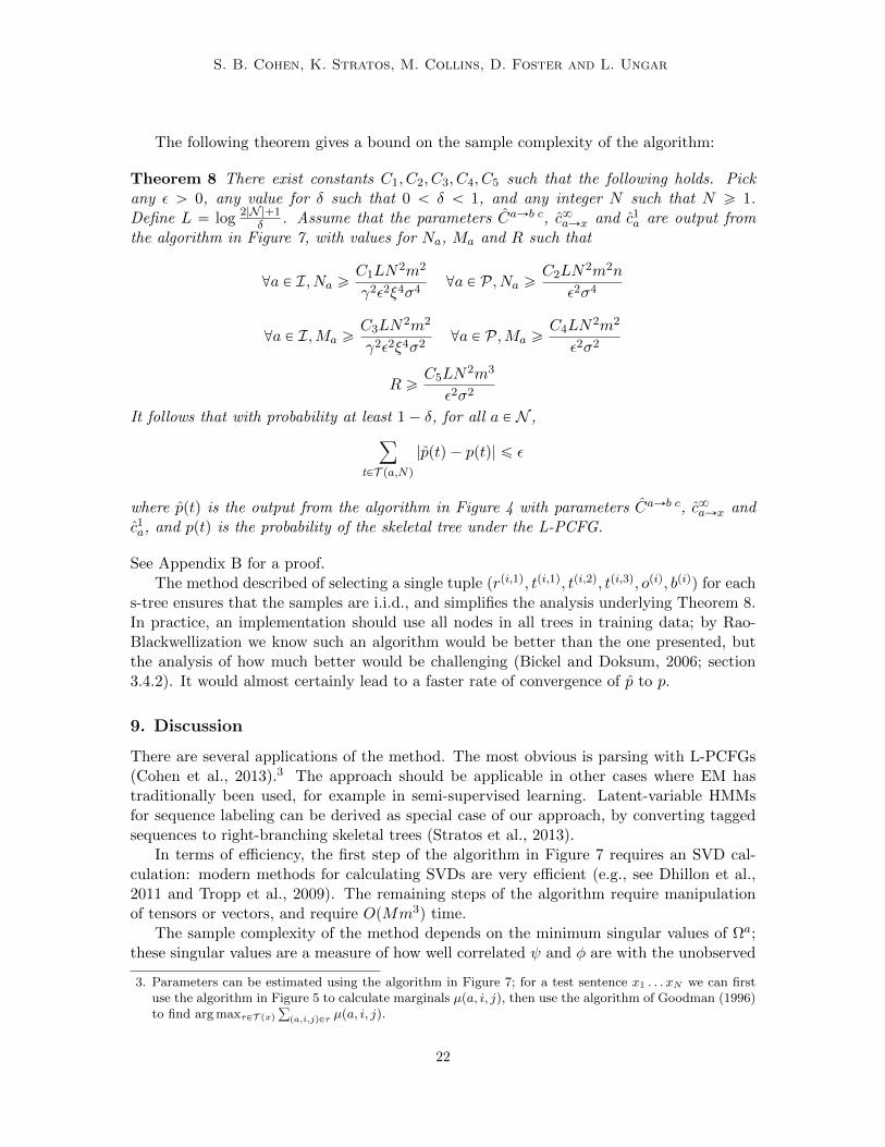
The following theorem gives a bound on the sample complexity of the algorithm:
Theorem 8 There exist constants C1, C2, C3, C4, C5 such that the following holds. Pickany ε ą 0, any value for δ such that 0 ă δ ă 1, and any integer N such that N ě 1.Define L “ log 2|N |`1
δ . Assume that the parameters CaÑb c, c8aÑx and c1a are output from
the algorithm in Figure 7, with values for Na, Ma and R such that
@a P I, Na ěC1LN
2m2
γ2ε2ξ4σ4@a P P, Na ě
C2LN2m2n
ε2σ4
@a P I,Ma ěC3LN
2m2
γ2ε2ξ4σ2@a P P,Ma ě
C4LN2m2
ε2σ2
R ěC5LN
2m3
ε2σ2
It follows that with probability at least 1´ δ, for all a P N ,
ÿ
tPT pa,Nq|pptq ´ pptq| ď ε
where pptq is the output from the algorithm in Figure 4 with parameters CaÑb c, c8aÑx andc1a, and pptq is the probability of the skeletal tree under the L-PCFG.
See Appendix B for a proof.The method described of selecting a single tuple prpi,1q, tpi,1q, tpi,2q, tpi,3q, opiq, bpiqq for each
s-tree ensures that the samples are i.i.d., and simplifies the analysis underlying Theorem 8.In practice, an implementation should use all nodes in all trees in training data; by Rao-Blackwellization we know such an algorithm would be better than the one presented, butthe analysis of how much better would be challenging (Bickel and Doksum, 2006; section3.4.2). It would almost certainly lead to a faster rate of convergence of p to p.
9. Discussion
There are several applications of the method. The most obvious is parsing with L-PCFGs(Cohen et al., 2013).3 The approach should be applicable in other cases where EM hastraditionally been used, for example in semi-supervised learning. Latent-variable HMMsfor sequence labeling can be derived as special case of our approach, by converting taggedsequences to right-branching skeletal trees (Stratos et al., 2013).
In terms of efficiency, the first step of the algorithm in Figure 7 requires an SVD cal-culation: modern methods for calculating SVDs are very efficient (e.g., see Dhillon et al.,2011 and Tropp et al., 2009). The remaining steps of the algorithm require manipulationof tensors or vectors, and require OpMm3q time.
The sample complexity of the method depends on the minimum singular values of Ωa;these singular values are a measure of how well correlated ψ and φ are with the unobserved
3. Parameters can be estimated using the algorithm in Figure 7; for a test sentence x1 . . . xN we can firstuse the algorithm in Figure 5 to calculate marginals µpa, i, jq, then use the algorithm of Goodman (1996)to find arg maxτPT pxq
ř
pa,i,jqPτ µpa, i, jq.
22
Spectral Learning of L-PCFGs: Algorithms and Sample Complexity
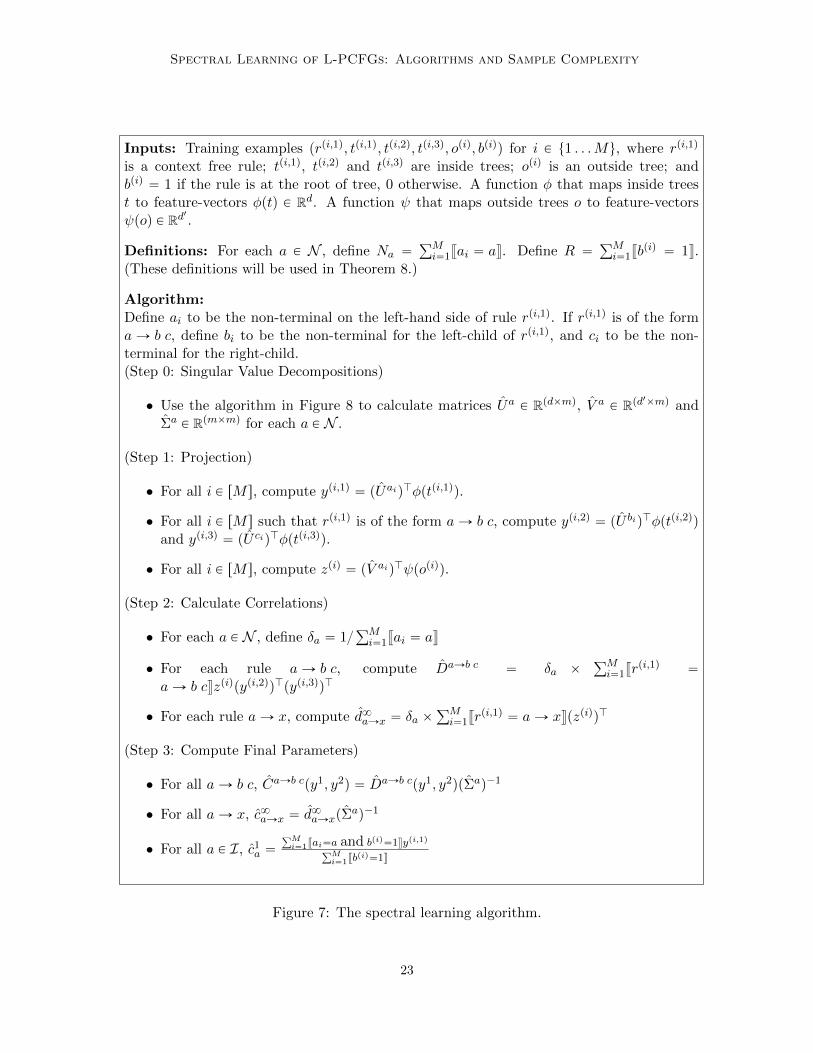
Inputs: Training examples prpi,1q, tpi,1q, tpi,2q, tpi,3q, opiq, bpiqq for i P t1 . . .Mu, where rpi,1q
is a context free rule; tpi,1q, tpi,2q and tpi,3q are inside trees; opiq is an outside tree; andbpiq “ 1 if the rule is at the root of tree, 0 otherwise. A function φ that maps inside treest to feature-vectors φptq P Rd. A function ψ that maps outside trees o to feature-vectorsψpoq P Rd
1
.
Definitions: For each a P N , define Na “řMi“1vai “ aw. Define R “
řMi“1vb
piq “ 1w.(These definitions will be used in Theorem 8.)
Algorithm:Define ai to be the non-terminal on the left-hand side of rule rpi,1q. If rpi,1q is of the formaÑ b c, define bi to be the non-terminal for the left-child of rpi,1q, and ci to be the non-terminal for the right-child.(Step 0: Singular Value Decompositions)
• Use the algorithm in Figure 8 to calculate matrices Ua P Rpdˆmq, V a P Rpd1ˆmq and
Σa P Rpmˆmq for each a P N .
(Step 1: Projection)
• For all i P rM s, compute ypi,1q “ pUaiqJφptpi,1qq.
• For all i P rM s such that rpi,1q is of the form aÑ b c, compute ypi,2q “ pU biqJφptpi,2qqand ypi,3q “ pU ciqJφptpi,3qq.
• For all i P rM s, compute zpiq “ pV aiqJψpopiqq.
(Step 2: Calculate Correlations)
• For each a P N , define δa “ 1řMi“1vai “ aw
• For each rule aÑ b c, compute DaÑb c “ δa ˆřMi“1vr
pi,1q “
aÑ b cwzpiqpypi,2qqJpypi,3qqJ
• For each rule aÑ x, compute d8aÑx “ δa ˆřMi“1vr
pi,1q “ aÑ xwpzpiqqJ
(Step 3: Compute Final Parameters)
• For all aÑ b c, CaÑb cpy1, y2q “ DaÑb cpy1, y2qpΣaq´1
• For all aÑ x, c8aÑx “ d8aÑxpΣaq´1
• For all a P I, c1a “
řMi“1vai“a and bpiq“1wypi,1q
řMi“1vb
piq“1w
Figure 7: The spectral learning algorithm.
23
S. B. Cohen, K. Stratos, M. Collins, D. Foster and L. Ungar
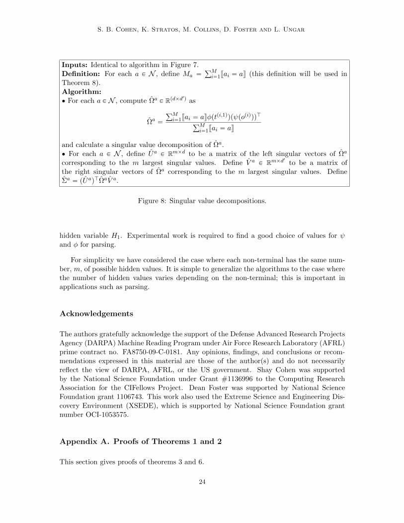
Inputs: Identical to algorithm in Figure 7.Definition: For each a P N , define Ma “
řMi“1vai “ aw (this definition will be used in
Theorem 8).Algorithm:‚ For each a P N , compute Ωa P Rpdˆd
1q as
Ωa “
řMi“1vai “ awφptpi,1qqpψpopiqqqJ
řMi“1vai “ aw
and calculate a singular value decomposition of Ωa.‚ For each a P N , define Ua P Rmˆd to be a matrix of the left singular vectors of Ωa
corresponding to the m largest singular values. Define V a P Rmˆd1
to be a matrix ofthe right singular vectors of Ωa corresponding to the m largest singular values. DefineΣa “ pUaqJΩaV a.
Figure 8: Singular value decompositions.
hidden variable H1. Experimental work is required to find a good choice of values for ψand φ for parsing.
For simplicity we have considered the case where each non-terminal has the same num-ber, m, of possible hidden values. It is simple to generalize the algorithms to the case wherethe number of hidden values varies depending on the non-terminal; this is important inapplications such as parsing.
Acknowledgements
The authors gratefully acknowledge the support of the Defense Advanced Research ProjectsAgency (DARPA) Machine Reading Program under Air Force Research Laboratory (AFRL)prime contract no. FA8750-09-C-0181. Any opinions, findings, and conclusions or recom-mendations expressed in this material are those of the author(s) and do not necessarilyreflect the view of DARPA, AFRL, or the US government. Shay Cohen was supportedby the National Science Foundation under Grant #1136996 to the Computing ResearchAssociation for the CIFellows Project. Dean Foster was supported by National ScienceFoundation grant 1106743. This work also used the Extreme Science and Engineering Dis-covery Environment (XSEDE), which is supported by National Science Foundation grantnumber OCI-1053575.
Appendix A. Proofs of Theorems 1 and 2
This section gives proofs of theorems 3 and 6.
24
Spectral Learning of L-PCFGs: Algorithms and Sample Complexity
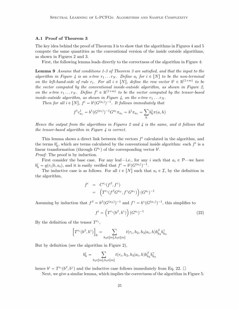
A.1 Proof of Theorem 3
The key idea behind the proof of Theorem 3 is to show that the algorithms in Figures 4 and 5compute the same quantities as the conventional version of the inside outside algorithms,as shown in Figures 2 and 3.
First, the following lemma leads directly to the correctness of the algorithm in Figure 4:
Lemma 9 Assume that conditions 1-3 of Theorem 3 are satisfied, and that the input to thealgorithm in Figure 4 is an s-tree r1 . . . rN . Define ai for i P rN s to be the non-terminalon the left-hand-side of rule ri. For all i P rN s, define the row vector bi P Rp1ˆmq to bethe vector computed by the conventional inside-outside algorithm, as shown in Figure 2,on the s-tree r1 . . . rN . Define f i P Rp1ˆmq to be the vector computed by the tensor-basedinside-outside algorithm, as shown in Figure 4, on the s-tree r1 . . . rN .
Then for all i P rN s, f i “ bipGpaiqq´1. It follows immediately that
f1c1a1 “ b1pGpa1qq´1Ga1πa1 “ b1πa1 “
ÿ
h
b1hπpa, hq
Hence the output from the algorithms in Figures 2 and 4 is the same, and it follows thatthe tensor-based algorithm in Figure 4 is correct.
This lemma shows a direct link between the vectors f i calculated in the algorithm, andthe terms bih, which are terms calculated by the conventional inside algorithm: each f i is alinear transformation (through Gai) of the corresponding vector bi.Proof: The proof is by induction.
First consider the base case. For any leaf—i.e., for any i such that ai P P—we havebih “ qpri|h, aiq, and it is easily verified that f i “ bipGpaiqq´1.
The inductive case is as follows. For all i P rN s such that ai P I, by the definition inthe algorithm,
f i “ Cripfβ, fγq
“
´
T ripfβGaβ , fγGaγ q¯
pGaiq´1
Assuming by induction that fβ “ bβpGpaβqq´1 and fγ “ bγpGpaγqq´1, this simplifies to
f i “´
T ripbβ, bγq¯
pGaiq´1 (22)
By the definition of the tensor T ri ,”
T ripbβ, bγqı
h“
ÿ
h2Prms,h3Prms
tpri, h2, h3|ai, hqbβh2bγh3
But by definition (see the algorithm in Figure 2),
bih “ÿ
h2Prms,h3Prms
tpri, h2, h3|ai, hqbβh2bγh3
hence bi “ T ripbβ, bγq and the inductive case follows immediately from Eq. 22.Next, we give a similar lemma, which implies the correctness of the algorithm in Figure 5:
25
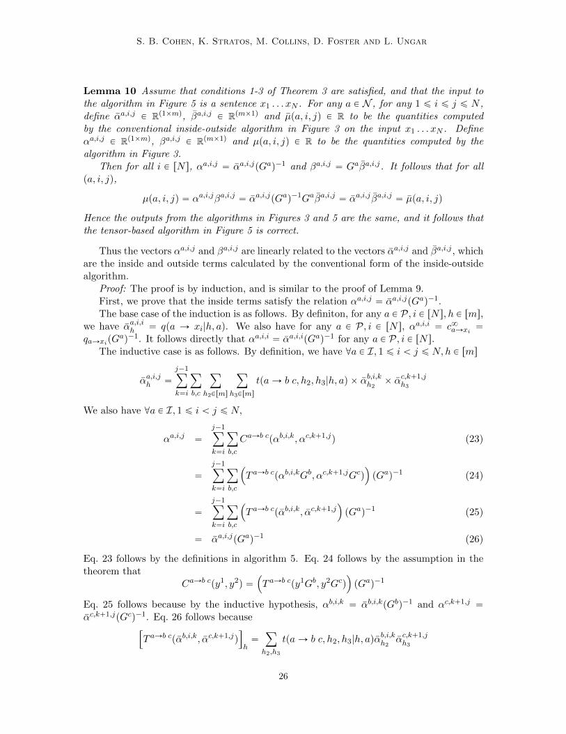
S. B. Cohen, K. Stratos, M. Collins, D. Foster and L. Ungar
Lemma 10 Assume that conditions 1-3 of Theorem 3 are satisfied, and that the input tothe algorithm in Figure 5 is a sentence x1 . . . xN . For any a P N , for any 1 ď i ď j ď N ,define αa,i,j P Rp1ˆmq, βa,i,j P Rpmˆ1q and µpa, i, jq P R to be the quantities computedby the conventional inside-outside algorithm in Figure 3 on the input x1 . . . xN . Defineαa,i,j P Rp1ˆmq, βa,i,j P Rpmˆ1q and µpa, i, jq P R to be the quantities computed by thealgorithm in Figure 3.
Then for all i P rN s, αa,i,j “ αa,i,jpGaq´1 and βa,i,j “ Gaβa,i,j. It follows that for allpa, i, jq,
µpa, i, jq “ αa,i,jβa,i,j “ αa,i,jpGaq´1Gaβa,i,j “ αa,i,j βa,i,j “ µpa, i, jq
Hence the outputs from the algorithms in Figures 3 and 5 are the same, and it follows thatthe tensor-based algorithm in Figure 5 is correct.
Thus the vectors αa,i,j and βa,i,j are linearly related to the vectors αa,i,j and βa,i,j , whichare the inside and outside terms calculated by the conventional form of the inside-outsidealgorithm.
Proof: The proof is by induction, and is similar to the proof of Lemma 9.First, we prove that the inside terms satisfy the relation αa,i,j “ αa,i,jpGaq´1.The base case of the induction is as follows. By definiton, for any a P P, i P rN s, h P rms,
we have αa,i,ih “ qpa Ñ xi|h, aq. We also have for any a P P, i P rN s, αa,i,i “ c8aÑxi “qaÑxipG
aq´1. It follows directly that αa,i,i “ αa,i,ipGaq´1 for any a P P, i P rN s.The inductive case is as follows. By definition, we have @a P I, 1 ď i ă j ď N,h P rms
αa,i,jh “
j´1ÿ
k“i
ÿ
b,c
ÿ
h2Prms
ÿ
h3Prms
tpaÑ b c, h2, h3|h, aq ˆ αb,i,kh2
ˆ αc,k`1,jh3
We also have @a P I, 1 ď i ă j ď N,
αa,i,j “
j´1ÿ
k“i
ÿ
b,c
CaÑb cpαb,i,k, αc,k`1,jq (23)
“
j´1ÿ
k“i
ÿ
b,c
´
T aÑb cpαb,i,kGb, αc,k`1,jGcq¯
pGaq´1 (24)
“
j´1ÿ
k“i
ÿ
b,c
´
T aÑb cpαb,i,k, αc,k`1,j¯
pGaq´1 (25)
“ αa,i,jpGaq´1 (26)
Eq. 23 follows by the definitions in algorithm 5. Eq. 24 follows by the assumption in thetheorem that
CaÑb cpy1, y2q “
´
T aÑb cpy1Gb, y2Gcq¯
pGaq´1
Eq. 25 follows because by the inductive hypothesis, αb,i,k “ αb,i,kpGbq´1 and αc,k`1,j “
αc,k`1,jpGcq´1. Eq. 26 follows because”
T aÑb cpαb,i,k, αc,k`1,jq
ı
h“
ÿ
h2,h3
tpaÑ b c, h2, h3|h, aqαb,i,kh2
αc,k`1,jh3
26
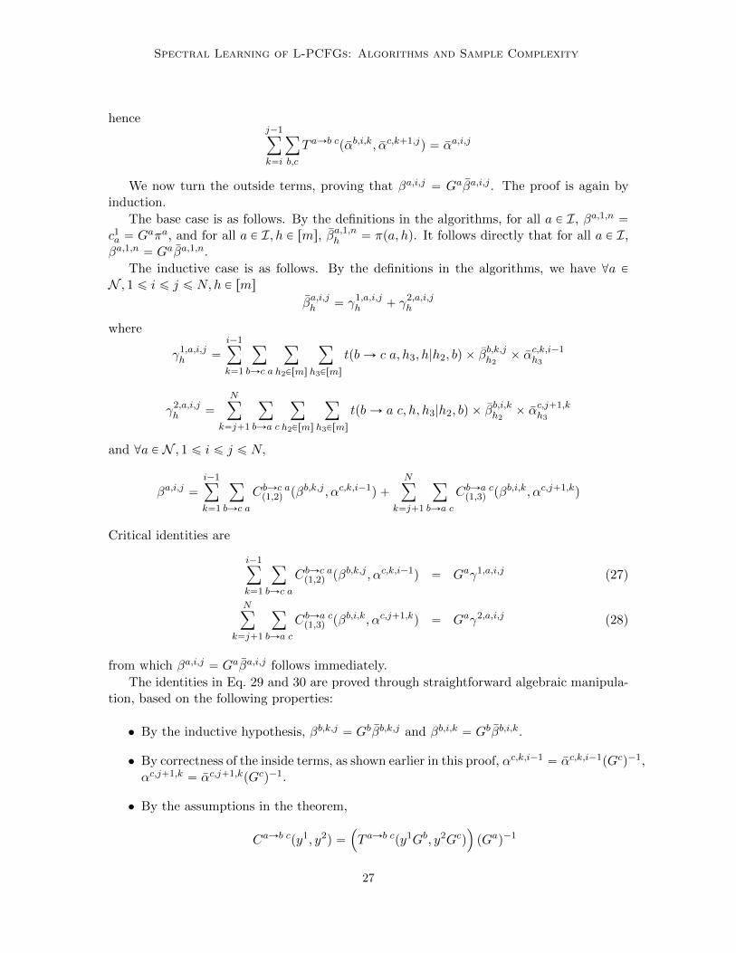
Spectral Learning of L-PCFGs: Algorithms and Sample Complexity
hencej´1ÿ
k“i
ÿ
b,c
T aÑb cpαb,i,k, αc,k`1,jq “ αa,i,j
We now turn the outside terms, proving that βa,i,j “ Gaβa,i,j . The proof is again byinduction.
The base case is as follows. By the definitions in the algorithms, for all a P I, βa,1,n “c1a “ Gaπa, and for all a P I, h P rms, βa,1,nh “ πpa, hq. It follows directly that for all a P I,βa,1,n “ Gaβa,1,n.
The inductive case is as follows. By the definitions in the algorithms, we have @a PN , 1 ď i ď j ď N,h P rms
βa,i,jh “ γ1,a,i,jh ` γ2,a,i,j
h
where
γ1,a,i,jh “
i´1ÿ
k“1
ÿ
bÑc a
ÿ
h2Prms
ÿ
h3Prms
tpbÑ c a, h3, h|h2, bq ˆ βb,k,jh2
ˆ αc,k,i´1h3
γ2,a,i,jh “
Nÿ
k“j`1
ÿ
bÑa c
ÿ
h2Prms
ÿ
h3Prms
tpbÑ a c, h, h3|h2, bq ˆ βb,i,kh2
ˆ αc,j`1,kh3
and @a P N , 1 ď i ď j ď N,
βa,i,j “i´1ÿ
k“1
ÿ
bÑc a
CbÑc ap1,2q pβb,k,j , αc,k,i´1q `
Nÿ
k“j`1
ÿ
bÑa c
CbÑa cp1,3q pβb,i,k, αc,j`1,kq
Critical identities are
i´1ÿ
k“1
ÿ
bÑc a
CbÑc ap1,2q pβb,k,j , αc,k,i´1q “ Gaγ1,a,i,j (27)
Nÿ
k“j`1
ÿ
bÑa c
CbÑa cp1,3q pβb,i,k, αc,j`1,kq “ Gaγ2,a,i,j (28)
from which βa,i,j “ Gaβa,i,j follows immediately.
The identities in Eq. 29 and 30 are proved through straightforward algebraic manipula-tion, based on the following properties:
• By the inductive hypothesis, βb,k,j “ Gbβb,k,j and βb,i,k “ Gbβb,i,k.
• By correctness of the inside terms, as shown earlier in this proof, αc,k,i´1 “ αc,k,i´1pGcq´1,αc,j`1,k “ αc,j`1,kpGcq´1.
• By the assumptions in the theorem,
CaÑb cpy1, y2q “
´
T aÑb cpy1Gb, y2Gcq¯
pGaq´1
27
S. B. Cohen, K. Stratos, M. Collins, D. Foster and L. Ungar
It follows (see Lemma 11) that
CbÑc ap1,2q pβb,k,j , αc,k,i´1q “ Ga
´
T bÑc ap1,2q ppGbq´1βb,k,j , αc,k,i´1Gcq
¯
“ Ga´
T bÑc ap1,2q pβb,k,j , αc,k,i´1q
¯
and
CbÑa cp1,3q pβb,i,k, αc,j`1,kq “ Ga
´
T bÑa cp1,3q pβb,i,k, αc,j`1,kq
¯
Finally, we give the following Lemma, as used above:
Lemma 11 Assume we have tensors C P Rmˆmˆm and T P Rmˆmˆm such that for anyy2, y3,
Cpy2, y3q “`
T py2A, y3Bq˘
D
where A,B,D are matrices in Rmˆm. Then for any y1, y2,
Cp1,2qpy1, y2q “ B
`
Tp1,2qpDy1, y2Aq
˘
(29)
and for any y1, y3,Cp1,3qpy
1, y3q “ A`
Tp1,3qpDy1, y3Bq
˘
(30)
Proof: Consider first Eq. 29. We will prove the following statement:
@y1, y2, y3, y3Cp1,2qpy1, y2q “ y3B
`
Tp1,2qpDy1, y2Aq
˘
This statement is equivalent to Eq. 29.First, for all y1, y2, y3, by the assumption that Cpy2, y3q “
`
T py2A, y3Bq˘
D,
Cpy2, y3qy1 “ T py2A, y3BqDy1
henceÿ
i,j,k
Ci,j,ky1i y
2j y
3k “
ÿ
i,j,k
Ti,j,kz1i z
2j z
3k (31)
where z1 “ Dy1, z2 “ y2A, z3 “ y3B.In addition, it is easily verified that
y3Cp1,2qpy1, y2q “
ÿ
i,j,k
Ci,j,ky1i y
2j y
3k (32)
y3B`
Tp1,2qpDy1, y2Aq
˘
“ÿ
i,j,k
Ti,j,kz1i z
2j z
3k (33)
where again z1 “ Dy1, z2 “ y2A, z3 “ y3B. Combining Eqs. 31, 32, and 33 gives
y3Cp1,2qpy1, y2q “ y3B
`
Tp1,2qpDy1, y2Aq
˘
thus proving the identity in Eq. 29.The proof of the identity in Eq. 30 is similar, and is omitted for brevity.
28
Spectral Learning of L-PCFGs: Algorithms and Sample Complexity
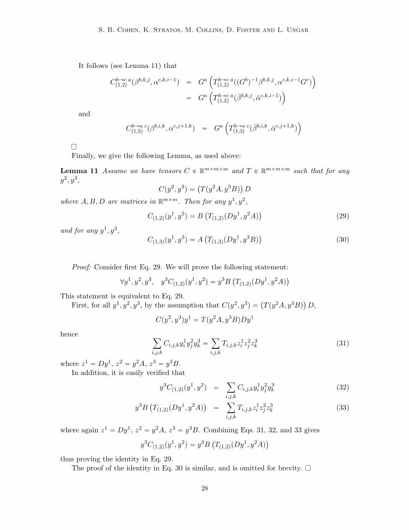
A.2 Proof of the Identity in Eq. 17
We now prove the identity in Eq. 17, repeated here:
DaÑb cpy1, y2q “
´
T aÑb cpy1Gb, y2Gcq¯
diagpγaqpKaqJ
Recall that
DaÑb c “ E“
vR1 “ aÑ b cwZY J2 YJ
3 |A1 “ a‰
or equivalently
DaÑb ci,j,k “ E rvR1 “ aÑ b cwZiY2,jY3,k|A1 “ as
Using the chain rule, and marginalizing over hidden variables, we have
DaÑb ci,j,k “ E rvR1 “ aÑ b cwZiY2,jY3,k|A1 “ as
“ÿ
h1,h2,h3Prms
ppaÑ b c, h1, h2, h3|aqE rZiY2,jY3,k|R1 “ aÑ b c, h1, h2, h3s
By definition, we have
ppaÑ b c, h1, h2, h3|aq “ γah1 ˆ tpaÑ b c, h2, h3|h1, aq
In addition, under the independence assumptions in the L-PCFG, and using the definitionsof Ka and Ga, we have
E rZiY2,jY3,k|R1 “ aÑ b c, h1, h2, h3s
“ E rZi|A1 “ a,H1 “ h1s ˆE rY2,j |A2 “ b,H2 “ h2s ˆE rY3,k|A3 “ c,H3 “ h3s
“ Kai,h1 ˆG
bj,h2 ˆG
ck,h3
Putting this all together gives
DaÑb ci,j,k “
ÿ
h1,h2,h3Prms
γah1 ˆ tpaÑ b c, h2, h3|h1, aq ˆKai,h1 ˆG
bj,h2 ˆG
ck,h3
“ÿ
h1Prms
γah1 ˆKai,h1 ˆ
ÿ
h2,h3Prms
tpaÑ b c, h2, h3|h1, aq ˆGbj,h2 ˆG
ck,h3
By the definition of tensors,
rDaÑb cpy1, y2qsi
“ÿ
j,k
DaÑb ci,j,k y1
j y2k
“ÿ
h1Prms
γah1 ˆKai,h1 ˆ
ÿ
h2,h3Prms
tpaÑ b c, h2, h3|h1, aq ˆ
˜
ÿ
j
y1jG
bj,h2
¸
ˆ
˜
ÿ
k
y2kG
ck,h3
¸
“ÿ
h1Prms
γah1 ˆKai,h1 ˆ
”
T aÑb cpy1Gb, y2Gcqı
h1(34)
29
S. B. Cohen, K. Stratos, M. Collins, D. Foster and L. Ungar
The last line follows because by the definition of tensors,”
T aÑb cpy1Gb, y2Gcqı
h1“
ÿ
h2,h3
T aÑb ch1,h2,h3
”
y1Gbı
h2
“
y2Gc‰
h3
and we have
T aÑb ch1,h2,h3 “ tpaÑ b c, h2, h3|h1, aq”
y1Gbı
h2“
ÿ
j
y1jG
bj,h2
“
y2Gc‰
h3“
ÿ
k
y2kG
ck,h3
Finally, the required identity
DaÑb cpy1, y2q “
´
T aÑb cpy1Gb, y2Gcq¯
diagpγaqpKaqJ
follows immediately from Eq. 34.
A.3 Proof of the Identity in Eq. 18
We now prove the identity in Eq. 18, repeated below:
d8aÑx “ qaÑxdiagpγaqpKaqJ
Recall that by definition
d8aÑx “ E“
vR1 “ aÑ xwZJ|A1 “ a‰
or equivalentlyrd8aÑxsi “ E rvR1 “ aÑ xwZi|A1 “ as
Marginalizing over hidden variables, we have
rd8aÑxsi “ E rvR1 “ aÑ xwZi|A1 “ as
“ÿ
h
ppaÑ x, h|aqErZi|H1 “ h,R1 “ aÑ xs
By definition, we have
ppaÑ x, h|aq “ γahqpaÑ x|h, aq “ γah rqaÑxsh
In addition, by the independence assumptions in the L-PCFG, and the definition of Ka,
ErZi|H1 “ h,R1 “ aÑ xs “ ErZi|H1 “ h,A1 “ as “ Kai,h
Putting this all together gives
rd8aÑxsi “ÿ
h
γah rqaÑxshKai,h
from which the required identity
d8aÑx “ qaÑxdiagpγaqpKaqJ
follows immediately.
30
Spectral Learning of L-PCFGs: Algorithms and Sample Complexity
A.4 Proof of the Identity in Eq. 19
We now prove the identity in Eq. 19, repeated below:
Σa “ GadiagpγaqpKaqJ
Recall that by definition
Σa “ ErY1ZJ|A1 “ as
or equivalently
rΣasi,j “ ErY1,iZj |A1 “ as
Marginalizing over hidden variables, we have
rΣasi,j “ ErY1,iZj |A1 “ as
“ÿ
h
pph|aqErY1,iZj |H1 “ h,A1 “ as
By definition, we have
γah “ pph|aq
In addition, under the independence assumptions in the L-PCFG, and using the definitionsof Ka and Ga, we have
ErY1,iZj |H1 “ h,A1 “ as “ ErY1,i|H1 “ h,A1 “ as ˆErZj |H1 “ h,A1 “ as
“ Gai,hKaj,h
Putting all this together gives
rΣasi,j “ÿ
h
γahGai,hK
aj,h
from which the required identity
Σa “ GadiagpγaqpKaqJ
follows immediately.
A.5 Proof of the Identity in Eq. 20
We now prove the identity in Eq. 19, repeated below:
c1a “ Gaπa
Recall that by definition
c1a “ E rvA1 “ awY1|B “ 1s
or equivalently
rc1asi “ E rvA1 “ awY1,i|B “ 1s
31
S. B. Cohen, K. Stratos, M. Collins, D. Foster and L. Ungar
Marginalizing over hidden variables, we have
rc1asi “ E rvA1 “ awY1,i|B “ 1s
“ÿ
h
P pA1 “ a,H1 “ h|B “ 1qE rY1,i|A1 “ a,H1 “ h,B “ 1s
By definition we have
P pA1 “ a,H1 “ h|B “ 1q “ πpa, hq
By the independence assumptions in the PCFG, and the definition of Ga, we have
E rY1,i|A1 “ a,H1 “ h,B “ 1s “ E rY1,i|A1 “ a,H1 “ hs
“ Gai,h
Putting this together gives
rc1asi “
ÿ
h
πpa, hqGai,h
from which the required identity
c1a “ Gaπa
follows.
Appendix B. Proof of Theorem 8
In this section we give a proof of Theorem 8. The proof relies on three lemmas:
• In Section B.1 we give a lemma showing that if estimates CaÑb c, caÑx and c1a are
close (up to linear transforms) to the parameters of an L-PCFG, then the distributiondefined by the parameters is close (in l1-norm) to the distribution under the L-PCFG.
• In Section B.2 we give a lemma showing that if the estimates Ωa, DaÑb c, d8aÑx andc1a are close to the underlying values being estimated, the estimates CaÑb c, caÑx andc1a are close (up to linear transforms) to the parameters of the underlying L-PCFG.
• In Section B.3 we give a lemma relating the number of samples in the estimationalgorithm to the errors in estimating Ωa, DaÑb c, d8aÑx and c1
a.
The proof of the theorem is then given in Section B.4.
B.1 A Bound on How Errors Propagate
In this section we show that if estimated tensors and vectors CaÑb c, c8aÑx and c1a are
sufficiently close to the underlying parameters T aÑb c, q8aÑx, and πa of an L-PCFG, thenthe distribution under the estimated parameters will be close to the distribution under theL-PCFG. Section B.1.1 gives assumptions and definitions; Lemma 12 then gives the mainlemma; the remainder of the section gives proofs.
32
Spectral Learning of L-PCFGs: Algorithms and Sample Complexity
B.1.1 Assumptions and Definitions
We make the following assumptions:
• Assume we have an L-PCFG with parameters T aÑb c P Rmˆmˆm, qaÑx P Rm, πa P Rm.Assume in addition that we have an invertible matrix Ga P Rmˆm for each a P N .For convenience define Ha “ pGaq´1 for all a P N .
• We assume that we have parameters CaÑb c P Rmˆmˆm, c8aÑx P R1ˆm and c1a P Rmˆ1
that satisfy the following conditions:
– There exists some constant ∆ ą 0 such that for all rules aÑ b c, for all y1, y2 P
Rm,||CaÑb cpy1Hb, y2HcqGa ´ T aÑb cpy1, y2q||8 ď ∆||y1||2||y
2||2
– There exists some constant δ ą 0 such that for all a P P, for all h P rms,ÿ
x
|rc8aÑxGash ´ rq
8aÑxsh| ď δ
– There exists some constant κ ą 0 such that for all a,
||pGaq´1c1a ´ π
a||1 ď κ
We give the following definitions:
• For any skeletal tree t “ r1 . . . rN , define biptq to be the quantities computed by thealgorithm in Figure 4 with t together with the parameters T aÑb c, q8aÑx, πa as input.Define f iptq to be the quantities computed by the algorithm in Figure 4 with t togetherwith the parameters CaÑb c, c8aÑx, c1
a as input. Define
ξptq “ b1ptq
andξptq “ f1ptqGa1
where as before a1 is the non-terminal on the left-hand-side of rule r1. Define pptq tobe the value returned by the algorithm in Figure 4 with t together with the parametersCaÑb c, c8aÑx, c1
a as input. Define pptq to be the value returned by the algorithm inFigure 4 with t together with the parameters T aÑb c, q8aÑx, πa as input.
• Define T pa,Nq to be the set of of all skeletal trees with N binary rules (hence 2N ` 1rules in total), with non-terminal a at the root of the tree.
• Define
Zpa, h,Nq “ÿ
tPT pa,Nqrξptqsh
Dpa, h,Nq “ÿ
tPT pa,Nq|rξptqsh ´ rξptqsh|
F pa, h,Nq “Dpa, h,Nq
Zpa, h,Nq
33
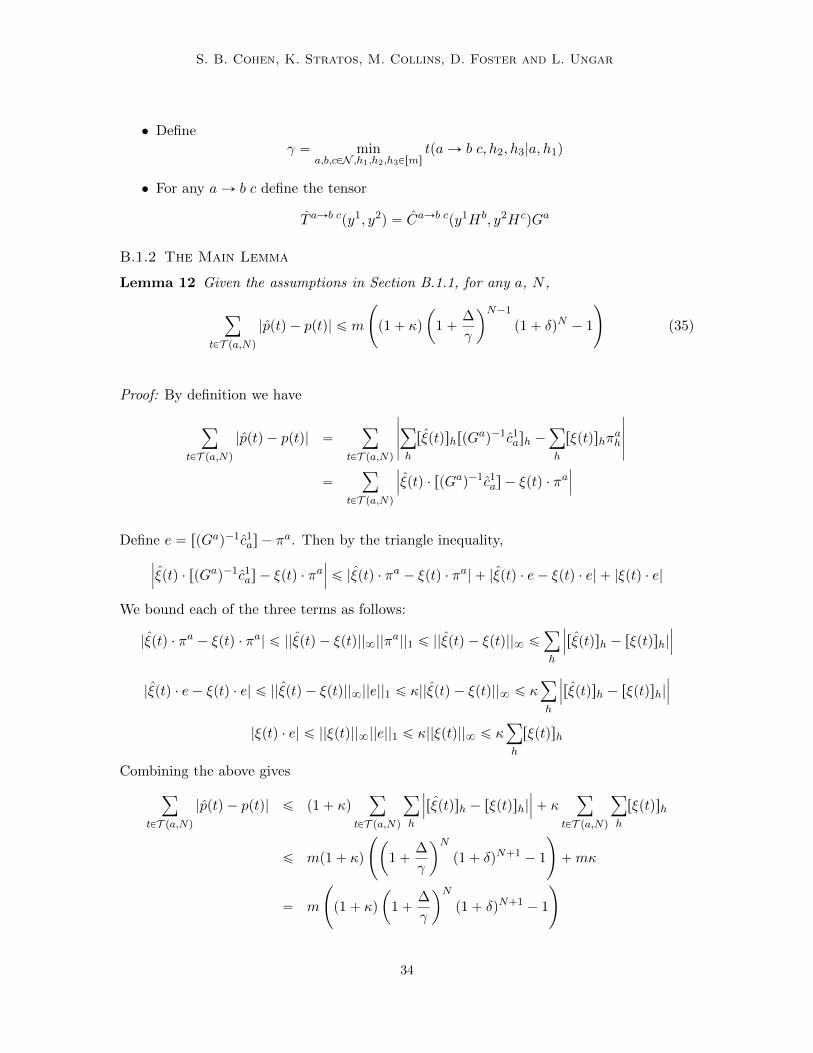
S. B. Cohen, K. Stratos, M. Collins, D. Foster and L. Ungar
• Defineγ “ min
a,b,cPN ,h1,h2,h3PrmstpaÑ b c, h2, h3|a, h1q
• For any aÑ b c define the tensor
T aÑb cpy1, y2q “ CaÑb cpy1Hb, y2HcqGa
B.1.2 The Main Lemma
Lemma 12 Given the assumptions in Section B.1.1, for any a, N ,
ÿ
tPT pa,Nq|pptq ´ pptq| ď m
˜
p1` κq
ˆ
1`∆
γ
˙N´1
p1` δqN ´ 1
¸
(35)
Proof: By definition we have
ÿ
tPT pa,Nq|pptq ´ pptq| “
ÿ
tPT pa,Nq
ˇ
ˇ
ˇ
ˇ
ˇ
ÿ
h
rξptqshrpGaq´1c1
ash ´ÿ
h
rξptqshπah
ˇ
ˇ
ˇ
ˇ
ˇ
“ÿ
tPT pa,Nq
ˇ
ˇ
ˇξptq ¨ rpGaq´1c1
as ´ ξptq ¨ πaˇ
ˇ
ˇ
Define e “ rpGaq´1c1as ´ π
a. Then by the triangle inequality,
ˇ
ˇ
ˇξptq ¨ rpGaq´1c1
as ´ ξptq ¨ πaˇ
ˇ
ˇď |ξptq ¨ πa ´ ξptq ¨ πa| ` |ξptq ¨ e´ ξptq ¨ e| ` |ξptq ¨ e|
We bound each of the three terms as follows:
|ξptq ¨ πa ´ ξptq ¨ πa| ď ||ξptq ´ ξptq||8||πa||1 ď ||ξptq ´ ξptq||8 ď
ÿ
h
ˇ
ˇ
ˇrξptqsh ´ rξptqsh|
ˇ
ˇ
ˇ
|ξptq ¨ e´ ξptq ¨ e| ď ||ξptq ´ ξptq||8||e||1 ď κ||ξptq ´ ξptq||8 ď κÿ
h
ˇ
ˇ
ˇrξptqsh ´ rξptqsh|
ˇ
ˇ
ˇ
|ξptq ¨ e| ď ||ξptq||8||e||1 ď κ||ξptq||8 ď κÿ
h
rξptqsh
Combining the above gives
ÿ
tPT pa,Nq|pptq ´ pptq| ď p1` κq
ÿ
tPT pa,Nq
ÿ
h
ˇ
ˇ
ˇrξptqsh ´ rξptqsh|
ˇ
ˇ
ˇ` κ
ÿ
tPT pa,Nq
ÿ
h
rξptqsh
ď mp1` κq
˜
ˆ
1`∆
γ
˙N
p1` δqN`1 ´ 1
¸
`mκ
“ m
˜
p1` κq
ˆ
1`∆
γ
˙N
p1` δqN`1 ´ 1
¸
34
Spectral Learning of L-PCFGs: Algorithms and Sample Complexity
where the second inequality follows becauseř
tPT pa,Nqř
hrξptqsh ď m, and because Lemma 13gives
ÿ
tPT pa,Nq
ÿ
h
ˇ
ˇ
ˇrξptqsh ´ rξptqsh|
ˇ
ˇ
ˇď m
˜
ˆ
1`∆
γ
˙N
p1` δqN`1 ´ 1
¸
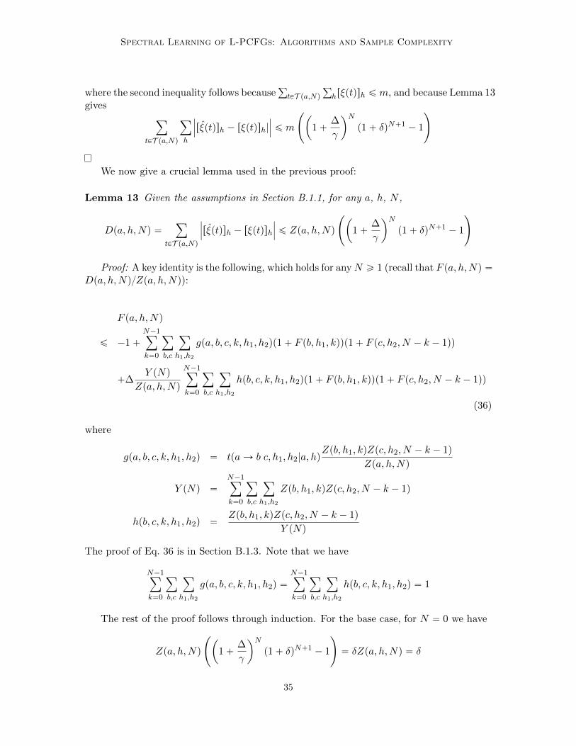
We now give a crucial lemma used in the previous proof:
Lemma 13 Given the assumptions in Section B.1.1, for any a, h, N ,
Dpa, h,Nq “ÿ
tPT pa,Nq
ˇ
ˇ
ˇrξptqsh ´ rξptqsh
ˇ
ˇ
ˇď Zpa, h,Nq
˜
ˆ
1`∆
γ
˙N
p1` δqN`1 ´ 1
¸
Proof: A key identity is the following, which holds for anyN ě 1 (recall that F pa, h,Nq “Dpa, h,NqZpa, h,Nq):
F pa, h,Nq
ď ´1`N´1ÿ
k“0
ÿ
b,c
ÿ
h1,h2
gpa, b, c, k, h1, h2qp1` F pb, h1, kqqp1` F pc, h2, N ´ k ´ 1qq
`∆Y pNq
Zpa, h,Nq
N´1ÿ
k“0
ÿ
b,c
ÿ
h1,h2
hpb, c, k, h1, h2qp1` F pb, h1, kqqp1` F pc, h2, N ´ k ´ 1qq
(36)
where
gpa, b, c, k, h1, h2q “ tpaÑ b c, h1, h2|a, hqZpb, h1, kqZpc, h2, N ´ k ´ 1q
Zpa, h,Nq
Y pNq “
N´1ÿ
k“0
ÿ
b,c
ÿ
h1,h2
Zpb, h1, kqZpc, h2, N ´ k ´ 1q
hpb, c, k, h1, h2q “Zpb, h1, kqZpc, h2, N ´ k ´ 1q
Y pNq
The proof of Eq. 36 is in Section B.1.3. Note that we have
N´1ÿ
k“0
ÿ
b,c
ÿ
h1,h2
gpa, b, c, k, h1, h2q “
N´1ÿ
k“0
ÿ
b,c
ÿ
h1,h2
hpb, c, k, h1, h2q “ 1
The rest of the proof follows through induction. For the base case, for N “ 0 we have
Zpa, h,Nq
˜
ˆ
1`∆
γ
˙N
p1` δqN`1 ´ 1
¸
“ δZpa, h,Nq “ δ
35
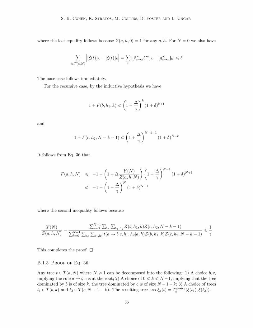
S. B. Cohen, K. Stratos, M. Collins, D. Foster and L. Ungar
where the last equality follows because Zpa, h, 0q “ 1 for any a, h. For N “ 0 we also have
ÿ
tPT pa,Nq
ˇ
ˇ
ˇrξptqsh ´ rξptqsh
ˇ
ˇ
ˇ“
ÿ
x
|rc8aÑxGash ´ rq
8aÑxsh| ď δ
The base case follows immediately.
For the recursive case, by the inductive hypothesis we have
1` F pb, h1, kq ď
ˆ
1`∆
γ
˙k
p1` δqk`1
and
1` F pc, h2, N ´ k ´ 1q ď
ˆ
1`∆
γ
˙N´k´1
p1` δqN´k
It follows from Eq. 36 that
F pa, h,Nq ď ´1`
ˆ
1`∆Y pNq
Zpa, h,Nq
˙ˆ
1`∆
γ
˙N´1
p1` δqN`1
ď ´1`
ˆ
1`∆
γ
˙N
p1` δqN`1
where the second inequality follows because
Y pNq
Zpa, h,Nq“
řN´1k“0
ř
b,c
ř
h1,h2Zpb, h1, kqZpc, h2, N ´ k ´ 1q
řN´1k“0
ř
b,c
ř
h1,h2tpaÑ b c, h1, h2|a, hqZpb, h1, kqZpc, h2, N ´ k ´ 1q
ď1
γ
This completes the proof.
B.1.3 Proof of Eq. 36
Any tree t P T pa,Nq where N ě 1 can be decomposed into the following: 1) A choice b, c,implying the rule aÑ b c is at the root; 2) A choice of 0 ď k ď N´1, implying that the treedominated by b is of size k, the tree dominated by c is of size N ´1´k; 3) A choice of treest1 P T pb, kq and t2 P T pc,N ´ 1´ kq. The resulting tree has ξhptq “ T aÑb ch pξpt1q, ξpt2qq.
36
Spectral Learning of L-PCFGs: Algorithms and Sample Complexity
Define dptq “ ξptq ´ ξptq. We then have the following:
ÿ
tPT pa,Nq|ξhptq ´ ξhptq|
“
N´1ÿ
k“0
ÿ
b,c
ÿ
t1PT pb,kq
ÿ
t2PT pc,N´1´kq
|T aÑb ch pξpt1q, ξpt2qq ´ TaÑb ch pξpt1q, ξpt2qq|
ď ∆N´1ÿ
k“0
ÿ
b,c
ÿ
t1PT pb,kq
ÿ
t2PT pc,N´1´kq
p||ξpt1q||2 ` ||dpt1q||2qp||ξpt2q||2 ` ||dpt2q||2q
`
N´1ÿ
k“0
ÿ
b,c
ÿ
t1PT pb,kq
ÿ
t2PT pc,N´1´kq
|T aÑb ch pξpt1q, dpt2qq|
`
N´1ÿ
k“0
ÿ
b,c
ÿ
t1PT pb,kq
ÿ
t2PT pc,N´1´kq
|T aÑb ch pdpt1q, ξpt2qq|
`
N´1ÿ
k“0
ÿ
b,c
ÿ
t1PT pb,kq
ÿ
t2PT pc,N´1´kq
|T aÑb ch pdpt1q, dpt2qq| (37)
The inequality follows because by Lemma 14,
|T aÑb ch pξpt1q, ξpt2qq ´ TaÑb ch pξpt1q, ξpt2qq|
ď ∆p||ξpt1q||2 ` ||dpt1q||2qp||ξpt2q||2 ` ||dpt2q||2q
`|T aÑb ch pξpt1q, dpt2qq| ` |TaÑb ch pdpt1q, ξpt2qq| ` |T
aÑb ch pdpt1q, dpt2qq|
We first derive an upper bound on the last three terms of Eq. 37. Note that we havethe identity
Zpa, h,Nq
“
N´1ÿ
k“0
ÿ
b,c
ÿ
h1,h2
tpaÑ b c, h1, h2|a, hqÿ
t1PT pb,kqξh1pt1q
ÿ
t2PT pc,N´1´kq
ξh2pt2q
“
N´1ÿ
k“0
ÿ
b,c
ÿ
h1,h2
tpaÑ b c, h1, h2|a, hqZpb, h1, kqZpc, h2, N ´ k ´ 1q
37
S. B. Cohen, K. Stratos, M. Collins, D. Foster and L. Ungar
It follows that
N´1ÿ
k“0
ÿ
b,c
ÿ
t1PT pb,kq
ÿ
t2PT pc,N´1´kq
`
|T aÑb ch pξpt1q, dpt2qq| ` |T
aÑb ch pdpt1q, ξpt2qq| ` |T
aÑb ch pdpt1q, dpt2qq|
˘
“
N´1ÿ
k“0
ÿ
b,c
ÿ
h1,h2
tpaÑ b c, h1, h2|a, hqÿ
t1PT pb,kq
ξpt1qh1
ÿ
t2PT pc,N´1´kq
|dpt2qh2|
`
N´1ÿ
k“0
ÿ
b,c
ÿ
h1,h2
tpaÑ b c, h1, h2|a, hqÿ
t1PT pb,kq
|dpt1qh1 |ÿ
t2PT pc,N´1´kq
ξpt2qh2
`
N´1ÿ
k“0
ÿ
b,c
ÿ
h1,h2
tpaÑ b c, h1, h2|a, hqÿ
t1PT pb,kq
|dpt1qh1|
ÿ
t2PT pc,N´1´kq
|dpt2qh2|
“
¨
˝
N´1ÿ
k“0
ÿ
b,c
ÿ
h1,h2
tpaÑ b c, h1, h2|a, hqÿ
t1PT pb,kq
ÿ
t2PT pc,N´1´kq
pξpt1qh1` |dpt1qh1
|qpξpt2qh2` |dpt2qh2
|q
˛
‚
´Zpa, h,Nq
“
˜
N´1ÿ
k“0
ÿ
b,c
ÿ
h1,h2
tpaÑ b c, h1, h2|a, hqpZpb, h1, kq `Dpb, h1, kqqpZpc, h2, N ´ k ´ 1q `Dpc, h2, N ´ k ´ 1qq
¸
´Zpa, h,Nq
“
˜
N´1ÿ
k“0
ÿ
b,c
ÿ
h1,h2
tpaÑ b c, h1, h2|a, hqZpb, h1, kqZpc, h2, N ´ k ´ 1qp1`Dpb, h1, kq
Zpb, h1, kqqp1`
Dpc, h2, N ´ k ´ 1q
Zpc, h2, N ´ k ´ 1q
¸
´Zpa, h,Nq
“ Zpa, h,Nq
˜
N´1ÿ
k“0
ÿ
b,c
ÿ
h1,h2
gpa, b, c, k, h1, h2qp1` F pb, h1, kqqp1` F pc, h2, N ´ k ´ 1qq
¸
´Zpa, h,Nq (38)
where gpa, b, c, k, h1, h2q “tpaÑb c,h1,h2|a,hqZpb,h1,kqZpc,h2,N´k´1q
Zpa,h,nq .
We next derive a bound on the first term as follows:
∆N´1ÿ
k“0
ÿ
b,c
ÿ
t1PT pb,kq
ÿ
t2PT pc,N´1´kq
p||ξpt1q||2 ` ||dpt1q||2qp||ξpt2q||2 ` ||dpt2q||2q
ď ∆N´1ÿ
k“0
ÿ
b,c
ÿ
t1PT pb,kq
ÿ
t2PT pc,N´1´kq
p||ξpt1q||1 ` ||dpt1q||1qp||ξpt2q||1 ` ||dpt2q||1q
“ ∆N´1ÿ
k“0
ÿ
b,c
ÿ
h1,h2
pZpb, h1, kq `Dpb, h1, kqqpZpc, h2, N ´ k ´ 1q `Dpc, h2, N ´ k ´ 1qq
“ ∆N´1ÿ
k“0
ÿ
b,c
ÿ
h1,h2
Zpb, h1, kqZpc, h2, N ´ k ´ 1qp1` F pb, h1, kqqp1` F pc, h2, N ´ k ´ 1qq
“ ∆Y pNqN´1ÿ
k“0
ÿ
b,c
ÿ
h1,h2
hpk, b, c, h1, h2qp1` F pb, h1, kqqp1` F pc, h2, N ´ k ´ 1qq (39)
38
Spectral Learning of L-PCFGs: Algorithms and Sample Complexity
where
hpk, b, c, h1, h2q “Zpb, h1, kqZpc, h2, N ´ k ´ 1q
Y pNq
and Y pNq “řN´1k“0
ř
b,c
ř
h1,h2Zpb, h1, kqZpc, h2, N ´ k ´ 1q.
Combining Eqs. 37, 38 and 39 gives the inequality in Eq. 36, repeated below:
F pa, h,Nq
ď ´1
`
N´1ÿ
k“0
ÿ
b,c
ÿ
h1,h2
gpa, b, c, k, h1, h2qp1` F pb, h1, kqqp1` F pc, h2, N ´ k ´ 1qq
`∆Y pNq
Zpa, h,Nq
N´1ÿ
k“0
ÿ
b,c
ÿ
h1,h2
hpb, c, k, h1, h2qp1` F pb, h1, kqqp1` F pc, h2, N ´ k ´ 1qq
The following lemma was used in the previous proof:
Lemma 14 Assume we have tensors T and T and that there is some constant ∆ such thatfor any y1, y2 P Rm,
||T py1, y2q ´ T py1, y2q||8 ď ∆||y1||2||y2||2
Then for any y1, y2, y1, y2, for any h, it follows that
|Thpy1, y2q ´ Thpy
1, y2q| ď ∆p||y1||2 ` ||d1||2qp||y
2||2 ` ||d2||2q
`|Thpy1, d2q| ` |Thpd
1, d2q| ` |Thpd1, y2q|
where d1 “ y1 ´ y1, and d2 “ y2 ´ y2.
Proof: Definegpy1q “ Thpy
1, y2q
gpy1q “ Thpy1, y2q
Define d1 “ py1 ´ y1q, d2 “ py2 ´ y2q. For any v P Rm,
|gpvq ´ gpvq| “ |Thpv, y2q ´ Thpv, y
2q|
ď |Thpv, y2q ´ Thpv, y
2q| ` |Thpv, d2q ´ Thpv, d
2q| ` |Thpv, d2q|
We can then derive the following bound:
|Thpy1, y2q ´ Thpy
1, y2q| “ |gpy1q ´ gpy1q|
ď |gpy1q ´ gpy1q| ` |gpd1q ´ gpd1q| ` |gpd1q|
ď |Thpy1, y2q ´ Thpy
1, y2q| ` |Thpy1, d2q ´ Thpy
1, d2q| ` |Thpy1, d2q|
`|Thpd1, y2q ´ Thpd
1, y2q| ` |Thpd1, d2q ´ Thpd
1, d2q| ` |Thpd1, d2q|
`|Thpd1, y2q|
ď ∆p||y1||2 ` ||d1||2qp||y
2||2 ` ||d2||2q
`|Thpy1, d2q| ` |Thpd
1, d2q| ` |Thpd1, y2q|
39
S. B. Cohen, K. Stratos, M. Collins, D. Foster and L. Ungar
B.2 Relating ∆, δ, κ to Estimation Errors
We now give a lemma that relates estimation errors in the algorithm to the values for ∆, δand κ as defined in the previous section.
Throughout this section, in addition to the estimates DaÑb c, d8aÑx, Σa, CaÑb c, c8aÑx,c1a computed by the algorithm in Figure 7, we define quantities
Σa “ ErY1ZJ|A1 “ as
DaÑb c “ E“
vR1 “ aÑ b cwZY J2 YJ
3 |A1 “ a‰
d8aÑx “ E“
vR1 “ aÑ xwZJ|A1 “ a‰
CaÑb cpy1, y2q “ DaÑb cpy1, y2qpΣaq´1
c8aÑx “ d8aÑxpΣaq´1
c1a “ E rvA1 “ awY1|B “ 1s
where
Y1 “ pUa1qJφpT1q Z “ pV
a1qJψpOq
Y2 “ pUa2qJφpT2q Y3 “ pU
a3qJφpT3q
Note that these definitions are identical to those given in Section 7.2, with the additionaldetail that the projection matrices used to define random variables Y1, Y2, Y3, Z are Ua andV a, that is, the projection matrices estimated in the first step of the algorithm in Figure 7.
The lemma is as follows:
Lemma 15 Assume that under a run of the algorithm in Figure 7 there are constantsε1Ω, ε
2Ω, εD, εd, επ such that
@a P P, ||Ωa ´ Ωa||F ď ε1Ω
@a P I, ||Ωa ´ Ωa||F ď ε2Ω
@aÑ b c, ||DaÑb c ´DaÑb c||F ď εD
@a P P,c
ÿ
x
||d8aÑx ´ d8aÑx||
22 ď εd
@a, ||c1a ´ c
1a||2 ď επ
Assume in addition that ε1Ω ď minaPPσmpΩaq
3 and ε2Ω ď minaPIσmpΩaq
3 . For all a define
Ga “ pUaqJIa and Ha “ pGaq´1. Then:
• For all a, Ga is invertible.
• For all y1, y2 P Rm, for all rules of the form aÑ b c
||CaÑb cpy1Hb, y2HcqGa ´ CaÑb cpy1Hb, y2HcqGa||8 ď ∆||y1||2||y2||2
where
∆ “16
3
1
σmpIbqσmpIcq
ˆ
ε2ΩσmpΩaq2
`εD
3σmpΩaq
˙
40
Spectral Learning of L-PCFGs: Algorithms and Sample Complexity
• For all a P P, for all h P rms,
ÿ
x
|rc8aÑxGash ´ rc
8aÑxG
ash| ď δ
where
δ “ 4
ˆ
ε1ΩσmpΩaq2
`εd?n
3σmpΩaq
˙
• For all a,
||pGaq´1c1a ´ pG
aq´1c1a||1 ď κ
where
κ “2?
3
?m
σmpΩaqεπ
B.2.1 Proof of Lemma 15
We first prove three necessary lemmas, then give a proof of Lemma 15.
Lemma 16 Assume we have vectors and matrices d P R1ˆm, Σ P Rmˆm, d P R1ˆm,Σ P Rmˆm, U P Rdˆm, I P Rdˆm. We assume that Σ, Σ, and pUJIq are invertible.
In addition define
c “ dΣ´1
c “ dΣ´1
Ga “ UJI
We assume:
• For h “ 1 . . .m, ||Ih||2 ď 1, where Ih is the h’th column of Ia.
• ||U ||2,o ď 1 where ||U ||2,o is the spectral norm of the matrix U .
• ||Σ´ Σ||2,o ď ε1
It follows that
||cGa ´ cGa||8 ď1`
?5
2
ε1||d||2
mintσmpΣq, σmpΣqu2`||d´ d||2σmpΣq
41
S. B. Cohen, K. Stratos, M. Collins, D. Foster and L. Ungar
Proof:
||cGa ´ cGa||8
“ ||pc´ cqUJI||8
(By definition Ga “ UJI)
ď ||pc´ cqUJ||2
(By ||Ih||2 ď 1)
ď ||c´ c||2
(By ||U ||2,o ď 1)
“ ||dΣ´1 ´ dΣ´1||2
(By definitions of c, c)
ď ||dpΣ´1 ´ Σ´1q||2 ` ||pd´ dqΣ´1||2
(By triangle inequality)
ď ||d||2||Σ´1 ´ Σ´1||2,o ` ||d´ d||2||Σ
´1||2,o
(By definition of ||.||2,o)
ď ||d||21`
?5
2
ε1
mintσmpΣq, σmpΣqu2`||d´ d||2σmpΣq
(By Lemma 23 of Hsu et al. (2009), and ||Σ´1||2,o “ 1σmpΣq)
Lemma 17 Assume we have vectors c, c P Rmˆ1, and we have a matrix Ga P Rmˆm thatis invertible. It follows that
||pGaq´1c´ pGaq´1c||1 ď
?m||c´ c||2σmpGaq
Proof:
||pGaq´1c´ pGaq´1c||1 ď?m||pGaq´1c´ pGaq´1c||2 ď
?m||c´ c||2σmpGaq
The first inequality follows because ||.||1 ď?m||.||2. The second inequality follows because
||pGaq´1||2,o “ 1σmpGaq.
Lemma 18 Assume we have matrices and tensors D P Rmˆmˆm, Σ P Rmˆm, D P Rmˆmˆm,Σ P Rmˆm, U P Rdˆm, I P Rdˆm, Gb P Rmˆm, Gc P Rmˆm. We assume that Σ, Σ, Gb, Gc,and UJI are invertible.
In addition define
Cpy1, y2q “ Dpy1, y2qΣ´1
Cpy1, y2q “ Dpy1, y2qΣ´1
Ga “ UJI
Hb “ pGbq´1
Hc “ pGcq´1
We assume:
42
Spectral Learning of L-PCFGs: Algorithms and Sample Complexity
• For h “ 1 . . .m, ||Ih||2 ď 1, where Ih is the h’th column of Ia.
• ||U ||2,o ď 1
• ||Σ´ Σ||2,o ď ε1
It follows that for any y1, y2 P Rm,
||Cpy1Hb, y2HcqGa ´ Cpy1Hb, y2HcqGa||8
ď||y1||2||y
2||2
σmpGbqσmpGcq
˜
1`?
5
2ˆ
ε1||D||F
mintσmpΣq, σmpΣqu2`||D ´D||FσmpΣq
¸
Proof:
||Cpy1Hb, y2HcqGa ´ Cpy1Hb, y2HcqGa||8
ď ||Dpy1Hb, y2Hcq||21`
?5
2
ε1
mintσmpΣq, σmpΣqu2`||Dpy1Hb, y2Hcq ´Dpy1Hb, y2Hcq||2
σmpΣq
(By Lemma 16, using d “ Dpy1Hb, y2Hcq, d “ Dpy1Hb, y2Hcq.)
ď ||y1Hb||2||y2Hc||2
˜
||D||F1`
?5
2
ε1
mintσmpΣq, σmpΣqu2`||D ´D||FσmpΣq
¸
(By ||Dpv1, v2q||2 ď ||D||F ||v1||2||v
2||2 for any tensor D, vectors v1, v2.)
ď||y1||2||y
2||2
σmpGbqσmpGcq
˜
||D||F1`
?5
2
ε1
mintσmpΣq, σmpΣqu2`||D ´D||FσmpΣq
¸
(By Hb “ pGbq´1 hence ||Hb||2,o “ 1σmpGbq. Similar for Hc.)
Proof of Lemma 15: By Lemma 9 of Hsu et al. (2009), assuming that εΩ ď minaσmpΩaq
3gives for all a
σmpΣaq ě
2
3σmpΩ
aq
σmpΣaq ě
?3
2σmpΩ
aq
σmpGaq ě
?3
2σmpI
aq
The condition that σmpIaq ą 0 implies that σmpG
aq ą 0 and hence Ga is invertible. Thevalues for ∆ and κ follow from lemmas 18 and and 17 respectively.
The value for δ is derived as follows. By Lemma 16 we have for any rule aÑ x, for anyh P rms,
|rc8aÑxGash ´ rc
8aÑxG
ash| ď1`
?5
2
ε1||d8aÑx||2
mintσmpΣaq, σmpΣaqu2`||d8aÑx ´ d
8aÑx||2
σmpΣaq(40)
By definition
d8aÑx “
˜
řMi“1vr
pi,1q “ aÑ xwřMi“1vai “ aw
¸
ˆ
˜
řMi“1vr
pi,1q “ aÑ xwpzpiqqJřMi“1vr
pi,1q “ aÑ xw
¸
43
S. B. Cohen, K. Stratos, M. Collins, D. Foster and L. Ungar
In addition zpiq “ pV aiqJψptpi,1qq and ||V ai ||2,o ď 1, ||ψptpi,1qq||2 ď 1, hence ||zpiq||2 ď 1, and
||d8aÑx||2 ď
řMi“1vr
pi,1q “ aÑ xwřMi“1vai “ aw
It follows thatÿ
x
||d8aÑx||2 ď 1 (41)
In addition we have
ÿ
x
||d8aÑx ´ d8aÑx||2 ď
?nc
ÿ
x
||d8aÑx ´ d8aÑx||
22 ď
?nεd (42)
Combining Eqs. 41, 42 and 40 gives for any a P P, for any h P rms,
ÿ
x
|rc8aÑxGash ´ rc
8aÑxG
ash| ď1`
?5
2
ε1
mintσmpΣaq, σmpΣaqu2`
?nb
ř
x ||d8aÑx ´ d
8aÑx||
22
σmpΣaq
from which the lemma follows.
B.3 Estimation Errors
The next lemma relates estimation errors to the number of samples in the algorithm inFigure 4:
Lemma 19 Consider the algorithm in Figure 7. With probability at least 1´δ, the followingstatements hold:
@a P I,d
ÿ
b,c
||DaÑb c ´DaÑb c||2F ď
c
1
Ma`
d
2
Malog
2|N | ` 1
δ
@a P P,c
ÿ
x
||d8aÑx ´ d8aÑx||
22 ď
c
1
Ma`
d
2
Malog
2|N | ` 1
δ
@a P N , ||Ωa ´ Ωa||F ď
c
1
Na`
d
2
Nalog
2|N | ` 1
δ
c
ÿ
a
||c1a ´ c
1a||
22 ď
c
1
R`
c
2
Rlog
2|N | ` 1
δ
44
Spectral Learning of L-PCFGs: Algorithms and Sample Complexity
B.3.1 Proof of Lemma 19
We first need the following lemma:
Lemma 20 Assume i.i.d. random vectors X1 . . . XN where each Xi P Rd, and for all i withprobability 1, ||Xi||2 ď 1. Define
q “ ErXis
for all i and
Q “
řNi“1Xi
N
Then for any ε ą 0,
Pp||Q´ q||2 ě 1?N ` εq ď e´Nε
22
Proof: The proof is very similar to the proof of proposition 19 of Hsu et al. (2009).Consider two random samples x1 . . . xn and y1 . . . yn where xi “ yi for all i ‰ k. define
q “
řNi“1 xiN
and
p “
řNi“1 yiN
Then
||q ´ q||2 ´ ||p´ q||2 ď ||q ´ p||2 “||xk ´ yk||2
Nď||xk||2 ` ||yk||2
Nď
2
N
It follows through McDiarmid’s inequality (McDiarmid, 1989) that
Prp||Q´ q||2 ě E||Q´ q||2 ` εq ď e´Nε22
45
S. B. Cohen, K. Stratos, M. Collins, D. Foster and L. Ungar
In addition,
E”
||Q´ q||2
ı
“ E
«
||
řNi“1Xi
N´ q||2
ff
“1
NE
«
||
Nÿ
i“1
pXi ´ qq||2
ff
ď1
N
g
f
f
eE
«
||
Nÿ
i“1
pXi ´ qq||22
ff
(By Jensen’s inequality)
“1
N
g
f
f
e
Nÿ
i“1
E“
||pXi ´ qq||22‰
(By independence of the Xi’s)
“1
N
g
f
f
e
Nÿ
i“1
E“
||Xi||22
‰
´N ||q||22
ď1
N
b
Np1´ ||q||22q
(By ||Xi||2 ď 1.)
ď1?N
which completes the proof.
Proof of Lemma 19: For each aÑ b c, i, j, k P rms, define a random variable
AaÑb ci,j,k “ vR1 “ aÑ b cwZiY2j Y
3k
It follows that
DaÑb ci,j,k “ ErAaÑb ci,j,k |A1 “ as
Note that
||Z||2 “ ||pVaqJψpOq||2 ď 1
because ||V a||2,o ď 1, and ||ψpOq||2 ď 1. Similarly ||Y 2||2 ď 1 and ||Y 3||2 ď 1.
In addition we have for all a P I,
ÿ
b,c
mÿ
i“1
mÿ
j“1
mÿ
k“1
|AaÑb ci,j,k |2 “ÿ
b,c
mÿ
i“1
mÿ
j“1
mÿ
k“1
|Zi|2|Y 2
j |2|Y 3
k |2vR1 “ aÑ b cw2
“ ||Z||22||Y2||22||Y
3||22pÿ
b,c
vR1 “ aÑ b cw2q ď 1
46
Spectral Learning of L-PCFGs: Algorithms and Sample Complexity
It follows by an application of Lemma 20 that for the definitions of DaÑb c and DaÑb c inFigure 7, for all a,
Pp
d
ÿ
b,c
ÿ
i,j,k
|DaÑb ci,j,k ´DaÑb c
i,j,k |2 ě 1a
Ma ` ε1q ď e´Maε212
or equivalently,
P
¨
˝
d
ÿ
b,c
||DaÑb c ´DaÑb c||2F ě1
?Ma
`
d
2
Malog
2|N | ` 1
δ
˛
‚ďδ
2|N | ` 1(43)
By a similar argument, if for each a P P, x P rns, i P rms we define the random variable
BaÑxi “ ZivR1 “ aÑ xw
then
d8aÑx “ ErBaÑxi |A1 “ as
andÿ
x
mÿ
i“1
|BaÑxi |2 “
ÿ
x
mÿ
i“1
|Zi|2vR1 “ aÑ xw2 ď 1
It follows by an application of Lemma 20 that for the definitions of d8aÑx and d8aÑx inFigure 7, for all a,
Pp
d
ÿ
x
ÿ
i
|rd8aÑxsi ´ rd8aÑxsi|
2 ě 1a
Na ` ε2q ď e´Maε222
or equivalently
P
˜
c
ÿ
x
||d8aÑx ´ d8aÑx||
22 ě
1?Ma
`
d
2
Malog
2|N | ` 1
δ
¸
ďδ
2|N | ` 1(44)
A similar argument can be used to show that for all a, for the definitions of Ωa and Ωa
in Figure 7,
Pp
d
ÿ
i,j
|Ωai,j ´ Ωa
i,j |2 ě 1
a
Na ` ε3q ď e´Naε232
or equivalently
P
˜
||Ωa ´ Ωa||F ě1
?Na
`
d
2
Nalog
2|N | ` 1
δ
¸
ďδ
2|N | ` 1(45)
Finally, if we define the random variable
F ai “ Y 1i vA1 “ aw
47
S. B. Cohen, K. Stratos, M. Collins, D. Foster and L. Ungar
thenÿ
a
ÿ
i
|F ai |2 “
ÿ
a
ÿ
i
|Y 1i |
2vA1 “ aw2 ď 1
In additionc1a “ ErF ai |B “ 1s
It follows by an application of Lemma 20 that for the definitions of c1a and c1
a in Figure 7,
Pp
d
ÿ
a
ÿ
i
|rc1asi ´ rc
1asi|
2 ě 1?R` ε4q ď e´Rε
242
or equivalently
P
˜
c
ÿ
a
||c1a ´ c
1a||
22 ě
1?R`
c
2
Rlog
2|N | ` 1
δ
¸
ďδ
2|N | ` 1(46)
Finally, applying the union bound to the 2|N | ` 1 events in Eqs. 43, 44, 45 and 46 provesthe theorem.
B.4 Proof of Theorem 8
Under the assumptions of the theorem, we have constants C1, C2, C3, C4 and C5 such that
@a P I, Na ě Lˆ
ˆ
C1N
γε
m
ξ2σ2
˙2
@a P P, Na ě Lˆ
ˆ
C2Nm
εσ2
˙2
@a P I,Ma ě Lˆ
ˆ
C3N
γε
m
ξ2σ
˙2
@a P P,Ma ě Lˆ
ˆ
C4Nm
?n
εσ
˙2
R ě Lˆ
ˆ
C5Nm
?m
εσ
˙2
It follows from Lemma 19 that with probability at least 1´ δ,
@a P I, ||Ωa ´ Ωa||F ď ε1Ω
@a P P, ||Ωa ´ Ωa||F ď ε2Ω
@aÑ b c, ||DaÑb c ´DaÑb c||F ď εD
@a P P,c
ÿ
x
||d8aÑx ´ d8aÑx||2 ď εd
@a, ||c1a ´ c
1a||2 ď επ
where
ε1Ω ď 3ˆ1
C2ˆ σ2 ˆ
ε
Nm
ε2Ω ď 3ˆ1
C1ˆ ξ2σ2 ˆ
γε
Nm
εD ď 3ˆ1
C3ˆ ξ2σ ˆ
γε
Nm
48
Spectral Learning of L-PCFGs: Algorithms and Sample Complexity
εd ď 3ˆ1
C4ˆ σ ˆ
ε?nNm
επ ď 3ˆ1
C5ˆ
σ?mˆ
ε
Nm
It follows from Lemma 15 that with suitable choices of C1 . . . C5, the inequalities in Lemma 15hold with values
∆ ďγε
4Nm
δ ďε
4Nm
κ ďε
4Nm
It follows from Lemma 12 that
ÿ
tPT pa,Nq|pptq ´ pptq| ď m
ˆ
´
1`ε
4Nm
¯2N´ 1
˙
ď ε
where the second inequality follows because p1` atqt ď 1` 2a for a ď 12.
References
S. Arora, R. Ge, Y. Halpern, D. M. Mimno, A. Moitra, D. Sontag, Y. Wu, and M. Zhu. Apractical algorithm for topic modeling with provable guarantees. In Proceedings of ICML,2013.
R. Bailly, A. Habrar, and F. Denis. A spectral approach for probabilistic grammaticalinference on trees. In Proceedings of ALT, 2010.
R. Bailly, Carreras P. X., F. M. Luque, and A. J. Quattoni. Unsupervised spectral learningof WCFG as low-rank matrix completion. In Proceedings of EMNLP, 2013.
J. Baker. Trainable Grammars for Speech Recognition. In Proceedings of ASA, 1979.
B. Balle, A. Quattoni, and X. Carreras. A spectral learning algorithm for finite statetransducers. In Proceedings of ECML, 2011.
P.J. Bickel and K.A. Doksum. Mathematical Statistics: Basic Ideas And Selected Topics.Mathematical Statistics: Basic Ideas and Selected Topics. Pearson Prentice Hall, 2006.
E. Charniak. Statistical Parsing with a Context-Free Grammar and Word Statistics. InProceedings of AAAI-IAAI, 1997.
S. B. Cohen and M. Collins. A provably correct learning algorithm for latent-variable pcfgs.In Proceedings of ACL, 2014.
S. B. Cohen, K. Stratos, M. Collins, D. P. Foster, and L. Ungar. Spectral learning oflatent-variable PCFGs. In Proceedings of ACL, 2012.
49
S. B. Cohen, K. Stratos, M. Collins, D. Foster and L. Ungar
S. B. Cohen, K. Stratos, M. Collins, D. P. Foster, and L. Ungar. Experiments with spectrallearning of latent-variable PCFGs. In Proceedings of NAACL, 2013.
M. Collins. Three generative, lexicalised models for statistical parsing. In Proceedings ofACL, 1997.
S. Dasgupta. Learning mixtures of Gaussians. In Proceedings of FOCS, 1999.
A. Dempster, N. Laird, and D. Rubin. Maximum likelihood estimation from incompletedata via the EM algorithm. Journal of the Royal Statistical Society B, 39:1–38, 1977.
P. Dhillon, D. Foster, and L. Ungar. Multi-view learning of word embeddings via CCA. InProceedings of NIPS, 2011.
P. Dhillon, J. Rodu, M. Collins, D. P. Foster, and L. H. Ungar. Spectral dependency parsingwith latent variables. In Proceedings of EMNLP, 2012.
D. P. Foster, J. Rodu, and L. H. Ungar. Spectral dimensionality reduction for HMMs.arXiv:1203.6130, 2012.
J. Goodman. Parsing algorithms and metrics. In Proceedings of ACL, 1996.
D. Hsu, S. M. Kakade, and T. Zhang. A spectral algorithm for learning hidden Markovmodels. In Proceedings of COLT, 2009.
H. Jaeger. Observable operator models for discrete stochastic time series. Neural Compu-tation, 12(6), 2000.
M. Johnson. PCFG Models of Linguistic Tree Representations. Computational Linguistics,24(4):613–632, 1998.
D. Klein and C.D. Manning. Accurate Unlexicalized Parsing. In Proceedings of ACL, pages423–430, 2003.
F. M. Luque, A. Quattoni, B. Balle, and X. Carreras. Spectral learning for non-deterministicdependency parsing. In Proceedings of EACL, 2012.
M.P. Marcus, B. Santorini, and M.A. Marcinkiewicz. Building a Large Annotated Corpusof English: The Penn Treebank. Computational Linguistics, 19(2):313–330, 1993.
T. Matsuzaki, Y. Miyao, and J. Tsujii. Probabilistic CFG with latent annotations. InProceedings of ACL, 2005.
C. McDiarmid. On the method of bounded differences. Surveys in Combinatorics, pages148–188, 1989.
A. Moitra and G. Valiant. Settling the polynomial learnability of mixtures of gaussians.IEEE Annual Symposium on Foundations of Computer Science, pages 93–102, 2010. ISSN0272-5428.
A. Parikh, L. Song, and E. P. Xing. A spectral algorithm for latent tree graphical models.In Proceedings of ICML, 2011.
50
Spectral Learning of L-PCFGs: Algorithms and Sample Complexity
S. Petrov, L. Barrett, R. Thibaux, and D. Klein. Learning accurate, compact, and inter-pretable tree annotation. In Proceedings of COLING-ACL, 2006.
S. Siddiqi, B. Boots, and G. Gordon. Reduced-rank hidden markov models. Journal ofMachine Learning Research, 9:741–748, 2010.
L. Song, B. Boots, S. M. Siddiqi, G. J. Gordon, and A. J. Smola. Hilbert space embeddingsof hidden Markov models. In Proceedings of ICML, 2010.
L. Song, A. P. Parikh, and E. P. Xing. Kernel embeddings of latent tree graphical models.In NIPS, pages 2708–2716, 2011.
K. Stratos, A. M. Rush, S. B. Cohen, and M. Collins. Spectral learning of refinementHMMs. In Proceedings of CoNLL, 2013.
S. A. Terwijn. On the learnability of hidden markov models. In Grammatical Inference: Al-gorithms and Applications (Amsterdam, 2002), volume 2484 of Lecture Notes in ArtificialIntelligence, pages 261–268, Berlin, 2002. Springer.
A. Tropp, N. Halko, and P. G. Martinsson. Finding structure with randomness: Stochasticalgorithms for constructing approximate matrix decompositions. In Technical Report No.2009-05, 2009.
L. Valiant. A theory of the learnable. Communications of the ACM, 27:1134–1142, 1984.
S. Vempala and G. Wang. A spectral algorithm for learning mixtures of distributions.Journal of Computer and System Sciences, 68(4):841–860, 2004.
51


