Download - OPTIMIZING MULTI-ITEM INVENTORY MANAGEMENT …

OPTIMIZING MULTI-ITEM INVENTORY
MANAGEMENT DECISIONS IN HEALTHCARE
FACILITIES
by
Nazanin Esmaili
Bachelor of Science, Sharif University of Technology, 2008
Master of Business Administration, Sharif University of Technology,
2011
Master of Science, University of Pittsburgh, 2013
Submitted to the Graduate Faculty of
the Swanson School of Engineering in partial fulfillment
of the requirements for the degree of
Doctor of Philosophy
University of Pittsburgh
2016

UNIVERSITY OF PITTSBURGH
SWANSON SCHOOL OF ENGINEERING
This dissertation was presented
by
Nazanin Esmaili
It was defended on
November 9, 2016
and approved by
Bryan A. Norman, PhD, Associate Professor, Industrial Engineering Department
Jayant Rajgopal, PhD, Professor, Industrial Engineering Department
Jerrold H. May, PhD, Professor, Joseph M. Katz Graduate School of Business
Oleg A. Prokopyev, PhD, Associate Professor, Industrial Engineering Department
Dissertation Co-Directors: Bryan A. Norman, PhD, Associate Professor, Industrial
Engineering Department,
Jayant Rajgopal, PhD, Professor, Industrial Engineering Department
ii

Copyright c© by Nazanin Esmaili
2016
iii

OPTIMIZING MULTI-ITEM INVENTORY MANAGEMENT DECISIONS
IN HEALTHCARE FACILITIES
Nazanin Esmaili, PhD
University of Pittsburgh, 2016
Healthcare costs in the United States continue to grow at a significant rate. In many
healthcare settings material supply and inventory management represent significant areas of
opportunity for managing healthcare costs more effectively. In this dissertation, we explore
three topics related to these areas.
In the first chapter, we propose methodologies to help clinicians store medications and
medical supplies optimally in space-constrained, decentralized Automated Dispensing Cab-
inets (ADCs) located on hospital patient floors. This is significant for many reasons: first,
locating and storing medical supplies and pharmaceutical products within automated dis-
pensing devices on patient floors is often not done efficiently and these devices are not utilized
optimally. The primary purpose of an ADC is to ensure ready access of pharmaceuticals
and medical supplies at floor locations within a hospital. However, the allocation of the
limited space within an ADC to these items is typically not planned systematically and this
often results in wasted staff effort as clinical personnel must expend effort in locating and
retrieving them from a hospital’s central pharmacy/storage location. A second major issue
in using these devices is human error associated with the selection of pharmaceuticals from
floor storage. These problems are addressed via two different mixed integer programming
(MIP) models. In the first model, we only focus on the tradeoff between storing many of a
few items and storing smaller quantities of many items and in the second model we also con-
sider how to reduce medication dispensing errors by designing appropriate storage layouts.
iv
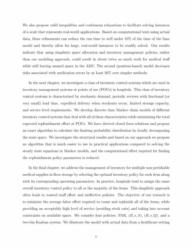
We also propose valid inequalities and continuous relaxations to facilitate solving instances
of a scale that represents real-world applications. Based on computational tests using actual
data, these refinements can reduce the run time to well under 10% of the time of the base
model and thereby allow for large, real-world instances to be readily solved. Our results
indicate that using simplistic space allocation and inventory management policies, rather
than our modeling approach, could result in about twice as much work for medical staff
while still leaving unused space in the ADC. The second (position-based) model decreases
risks associated with medication errors by at least 38% over simpler methods.
In the next chapter, we investigate a class of inventory control systems which are used in
inventory management systems at points of use (POUs) in hospitals. This class of inventory
control systems is characterized by stochastic demand, periodic reviews with fractional (or
very small) lead time, expedited delivery when stockouts occur, limited storage capacity,
and service level requirements. We develop discrete time Markov chain models of different
inventory control systems that deal with all of these characteristics while minimizing the total
expected replenishment effort at POUs. We have derived closed form solutions and propose
an exact algorithm to calculate the limiting probability distribution by locally decomposing
the state space. We investigate the structural results and based on our approach we propose
an algorithm that is much easier to use in practical applications compared to solving the
steady state equations in Markov models, and the computational effort required for finding
the replenishment policy parameters is reduced.
In the final chapter, we address the management of inventory for multiple non-perishable
medical supplies in floor storage by selecting the optimal inventory policy for each item along
with its corresponding operating parameters. In practice, hospitals tend to assign the same
overall inventory control policy to all or the majority of the items. This simplistic approach
often leads to wasted staff effort and ineffective policies. The objective of our research is
to minimize the average labor effort required to count and replenish all of the items, while
providing an acceptably high level of service (avoiding stock outs) and taking into account
constraints on available space. We consider four policies: PAR, (R, s, S), (R, s,Q), and a
two-bin Kanban system. We illustrate the model with actual data from a healthcare setting
v
and propose some practical insights and guidelines on how to choose a hybrid inventory
system based on demand and system characteristics.
Keywords: Mixed integer programming, computational optimization, two-staged two di-
mensional knapsack problem, valid inequalities, healthcare operations, automated dispensing
cabinets (ADCs), discrete time Markov chains, local decomposition, closed form solutions
hybrid inventory control system, periodic inventory policies, expedited deliveries, point of
use locations
vi

TABLE OF CONTENTS
PREFACE . . . . . . . . . . . . . . . . . . . . . . . . . . . . . . . . . . . . . . . . . xiv
1.0 INTRODUCTION . . . . . . . . . . . . . . . . . . . . . . . . . . . . . . . . . 1
2.0 SHELF-SPACE OPTIMIZATION MODELS IN DECENTRALIZED
AUTOMATED DISPENSING DEVICES . . . . . . . . . . . . . . . . . . 3
2.1 INTRODUCTION . . . . . . . . . . . . . . . . . . . . . . . . . . . . . . . . 3
2.2 LITERATURE REVIEW . . . . . . . . . . . . . . . . . . . . . . . . . . . . 8
2.3 MODEL DEVELOPMENT . . . . . . . . . . . . . . . . . . . . . . . . . . . 11
2.3.1 A Position-Free Paradigm . . . . . . . . . . . . . . . . . . . . . . . . . 15
2.3.2 A Position-Based Paradigm . . . . . . . . . . . . . . . . . . . . . . . . 18
2.4 TIGHTENING AND ENHANCING THE MIP FORMULATIONS . . . . . 22
2.5 COMPUTATIONAL ANALYSIS . . . . . . . . . . . . . . . . . . . . . . . . 27
2.5.1 Analysis of Valid Inequalities . . . . . . . . . . . . . . . . . . . . . . . 27
2.5.2 Benchmarking . . . . . . . . . . . . . . . . . . . . . . . . . . . . . . . 31
2.5.3 Contrasting MIP1 and MIP2 . . . . . . . . . . . . . . . . . . . . . . . 34
2.6 CONCLUSIONS . . . . . . . . . . . . . . . . . . . . . . . . . . . . . . . . . 37
vii
3.0 CLOSED-FORM SOLUTIONS FOR PERIODIC INVENTORY SYS-
TEMS WITH FRACTIONAL LEAD TIME, LOST SALES AND SER-
VICE LEVEL RESTRICTIONS . . . . . . . . . . . . . . . . . . . . . . . . 40
3.1 INTRODUCTION . . . . . . . . . . . . . . . . . . . . . . . . . . . . . . . . 40
3.2 LITERATURE REVIEW . . . . . . . . . . . . . . . . . . . . . . . . . . . . 41
3.3 MARKOV CHAIN MODEL FORMULATION . . . . . . . . . . . . . . . . 44
3.4 STRUCTURAL RESULTS . . . . . . . . . . . . . . . . . . . . . . . . . . . 50
3.4.1 Structural Results for the (R, s, S) Policy . . . . . . . . . . . . . . . . 54
3.4.2 Structural Results for the (R, s,Q) Policy . . . . . . . . . . . . . . . . 67
3.5 NUMERICAL ANALYSIS . . . . . . . . . . . . . . . . . . . . . . . . . . . . 76
3.5.1 Analyzing the Relationship Between Lead Time and Service Level . . 77
3.5.2 Trade-offs Between Replenishment Effort and Service Level for (R, s, S)
and (R, s,Q) Policies . . . . . . . . . . . . . . . . . . . . . . . . . . . 79
3.5.3 Reorder Points and Service Levels in the (R, s,Q) Policy . . . . . . . 80
3.5.4 Computational Effort and Problem Size . . . . . . . . . . . . . . . . . 84
3.5.5 Illustration of Algorithm 1 . . . . . . . . . . . . . . . . . . . . . . . . 85
3.6 CONCLUSIONS . . . . . . . . . . . . . . . . . . . . . . . . . . . . . . . . . 88
4.0 OPTIMAL SELECTION OF INVENTORY POLICIES IN A HEALTH-
CARE SETTING WITH SERVICE LEVEL AND SPACE CONSTRAINTS 89
4.1 INTRODUCTION . . . . . . . . . . . . . . . . . . . . . . . . . . . . . . . . 89
4.2 LITERATURE REVIEW . . . . . . . . . . . . . . . . . . . . . . . . . . . . 90
4.3 COMPARISON OF DIFFERENT INVENTORY POLICIES IN HOSPITALS 93
viii

4.4 MODEL AND ALGORITHM DEVELOPMENTS . . . . . . . . . . . . . . 97
4.5 OPTIMAL ALLOCATION MODELS BASED ON REPLENISHMENT EF-
FORT . . . . . . . . . . . . . . . . . . . . . . . . . . . . . . . . . . . . . . . 105
4.6 COMPUTATIONAL ANALYSIS . . . . . . . . . . . . . . . . . . . . . . . . 106
4.6.1 Trade-offs Between (R, s, S) and (R, s,Q) . . . . . . . . . . . . . . . . 106
4.6.2 Sensitivity Analysis for Service Level Across All Policies . . . . . . . . 111
4.6.3 Optimal Allocation Based on Changing Available Storage Space . . . 113
4.6.4 Tradeoffs Between Different Policies Considering Different Inventory
Control Parameter Settings . . . . . . . . . . . . . . . . . . . . . . . . 117
4.7 SUMMARY AND CONCLUSIONS . . . . . . . . . . . . . . . . . . . . . . . 123
5.0 CONCLUSIONS AND FUTURE WORK . . . . . . . . . . . . . . . . . . 124
APPENDIX A. LM MODEL ADOPTION TO MIP1 . . . . . . . . . . . . . . 130
APPENDIX B. EXAMPLE OF (R, S, S) AND (R, S,Q) PROBABILITY
TRANSITION MATRICES . . . . . . . . . . . . . . . . . . . . . . . . . . . 132
BIBLIOGRAPHY . . . . . . . . . . . . . . . . . . . . . . . . . . . . . . . . . . . . 134
ix

LIST OF TABLES
1 ADC transaction data set characteristics and number of medication pairs based
on different similarity factors . . . . . . . . . . . . . . . . . . . . . . . . . . . 28
2 Summary of valid inequalities effects for Model MIP2 considering different
percentages of nonadjacent medication pairs on and between shelves . . . . . 32
3 Comparison of heuristic versus optimal methods for MIP1 . . . . . . . . . . . 34
4 Medication categorical data: an example . . . . . . . . . . . . . . . . . . . . 37
5 Example of algorithm iterations . . . . . . . . . . . . . . . . . . . . . . . . . 86
6 Characteristics of the relevant literature in periodic review inventory system
in hospitals . . . . . . . . . . . . . . . . . . . . . . . . . . . . . . . . . . . . . 92
7 Summary of sets and indices used for the models . . . . . . . . . . . . . . . . 98
8 Parameters for deriving objective function coefficients . . . . . . . . . . . . . 99
9 Summary of parameters needed for the models . . . . . . . . . . . . . . . . . 103
10 Summary of service level for PAR and Kanban policy . . . . . . . . . . . . . 113
11 Optimal values from Model 2LBP . . . . . . . . . . . . . . . . . . . . . . . . . . 115
x
LIST OF FIGURES
1 (a) Tower module ADC (OmniRx one cell, courtesy of Omnicell company) (b)
Schematic figure of OmniRx (c) MIP model display. . . . . . . . . . . . . . . 12
2 (a) 24 compartment matrix drawer (b) General MIP model display (c) MIP
model display configuration . . . . . . . . . . . . . . . . . . . . . . . . . . . . 13
3 ADC transaction data set characteristics and number of medication pairs based
on different similarity factors . . . . . . . . . . . . . . . . . . . . . . . . . . . 29
4 Runtime with different combinations of valid inequalities, as a fraction of run-
time without valid inequalities (double column ADC) . . . . . . . . . . . . . 30
5 Performance profiles for MIP1 as percentages of those of the LM adaptation . 35
6 (a) A layout from MIP1 (LTE=3.5), (b) Layout after initial reordering (LTE=2.37),
(c) Layout after further reordering (LTE=1.17), (d) Layout from MIP2 (LTE=0.04) 38
7 The healthcare supply chain system of interest . . . . . . . . . . . . . . . . . 41
8 Sample path of on-hand inventory level in a periodic review system with lost
sales and fractional lead time. . . . . . . . . . . . . . . . . . . . . . . . . . . . 46
9 Comparison of (R, s, S) and (R, s,Q) policies service level whenD ∼ Poisson(µ =
10), and C = 15 and (a) L=0, (b)E[DL] = 1 (c)E[DL] = 7 in increasing order
of reorder points . . . . . . . . . . . . . . . . . . . . . . . . . . . . . . . . . . 78
xi
10 Inventory policy performance for L = 0, D ∼ Poisson(µ = 5), and C = 15 in
increasing order of reorder points . . . . . . . . . . . . . . . . . . . . . . . . . 79
11 Inventory policy performance for L = 0, D ∼ Poisson(µ = 10), and C = 15 in
increasing order of reorder points . . . . . . . . . . . . . . . . . . . . . . . . . 80
12 Inventory position analysis for L = 0, D ∼ Poisson(µ = 5), and C = 15 . . . . 82
13 Inventory position analysis for L = 0, D ∼ Poisson(µ = 10), and C = 15 . . . 83
14 Percentage reduction in matrix size by applying Theorem 5 . . . . . . . . . . 84
15 Schematic view of the transition matrix of the algorithm. Each color represents
a different value. . . . . . . . . . . . . . . . . . . . . . . . . . . . . . . . . . . 87
16 Comparison of (R, s, S) and (R, s,Q) policies (a) expected counting effort, (b)
expected reordering effort, and (c) α-service level when D ∼ Poisson(µ = 5),
L = 0, and C = 15 in increasing order of reorder points. . . . . . . . . . . . . 108
17 Comparison of (R, s, S) and (R, s,Q) policies (a) expected counting effort, (b)
expected reordering effort, and (c) service level when D ∼ Poisson(µ = 10),
L = 0, and C = 15 in increasing order of reorder points. . . . . . . . . . . . . 108
18 Comparison of (R, s, S) and (R, s,Q) policies (a) expected counting effort, (b)
expected reordering effort, and (c) service level when D ∼ Poisson(µ = 5),
E[DL] = 1, and C = 15 in increasing order of reorder points. . . . . . . . . . 109
19 Comparison of (R, s, S) and (R, s,Q) policies (a) expected counting effort, (b)
expected reordering effort, and (c) service level when D ∼ Poisson(µ = 10),
E[DL] = 1, and C = 15 in increasing order of reorder points. . . . . . . . . . 109
20 Limiting probabilities for different on-hand inventory levels; D ∼ Poisson(µ = 5)110
21 Limiting probabilities for different on-hand inventory levels; D ∼ Poisson(µ =
10) . . . . . . . . . . . . . . . . . . . . . . . . . . . . . . . . . . . . . . . . . 111
xii

22 Optimal reorder point for an (R, s, S) policy over different α service level
thresholds . . . . . . . . . . . . . . . . . . . . . . . . . . . . . . . . . . . . . 112
23 Optimal reorder point for an (R, s,Q) policy over different α service level
thresholds . . . . . . . . . . . . . . . . . . . . . . . . . . . . . . . . . . . . . 112
24 Optimal policy based on the number of shelves and item characteristics for a
sample of 20 items . . . . . . . . . . . . . . . . . . . . . . . . . . . . . . . . . 116
25 Randomly generated item bin size and demand data . . . . . . . . . . . . . . 118
26 Distribution of inventory systems when the number of shelves increases for (a)
setting 1 (b) setting 2 (c) setting 3 . . . . . . . . . . . . . . . . . . . . . . . . 119
27 Distribution of the maximum inventory on-hand when the number of shelves
increases for (a) setting 1 (b) setting 2 (c) setting 3 . . . . . . . . . . . . . . . 120
28 Total cost when the number of shelves increases for (a) setting 1 (b) setting 2
(c) setting 3 . . . . . . . . . . . . . . . . . . . . . . . . . . . . . . . . . . . . 121
xiii

PREFACE
Firstly, I would like to express my sincere gratitude to my advisors Professors Bryan
Norman and Jayant Rajgopal for the continuous support of my Ph.D. study, for their pa-
tience, motivation, and immense knowledge. None of this work would have been possible
without their guidance and constructive feedback. In addition to my advisors, I would like
to thank the other members of my dissertation committee, Professors Jerold May, and Oleg
Prokopyev, for their insightful comments and support.
I would like to extend my deepest gratitude to the chair of the Department of Industrial
Engineering, Professor Bopaya Bidanda for his unconditional support and advice throughout
my Ph.D. studies. I would also like to express my sincere appreciation to our wonderful
collaborator Mr. Robert Monte, for his kind support when it was needed.
I would like to express my genuine appreciation to Professor Jeffrey Kharoufeh for his
continuous support, time, and advice during my Ph.D. studies. I am also very thankful to
Professor Mor Harchol-Balter for her valuable suggestions, insights and time. Moreover, I
am grateful to Professor Jennifer Pazour for providing the data sets used for testing one of
my models.
Last but not least, I want to dedicate this dissertation to my parents, Giti and Abbas,
for loving me unconditionally, taking care of me even across the other side of the world and
for supporting every single decision that I have made. Above all, I would like to thank my
best friend, the love of my life, my husband, Pouyan for his unconditional love and support.
xiv
1.0 INTRODUCTION
Providing high quality and affordable health care is one of the greatest challenges facing
the nations of the world (Hall 2012). Since the 90s, the health care sector has changed
rapidly. Due to increased competition, and a stronger necessity to deliver health services in
a more efficient and effective way, many health care organizations have started projects in
the area of service quality, clinical pathways, information systems and logistics [Stock et al.
(2007)]. Nevertheless hospitals carry large amounts of a great variety of items, and health
care organizations have paid little attention to the management of inventories [Nicholson
et al. (2004)]. Studies performed in the past as well as more recent research suggest that
inventory costs in the health care sector are substantial and are estimated to be between
10% and 18% of net revenues (De Vries 2011). At the same time, hospitals are trying to
increase their internal service performance and this is another reason why a strong focus
on inventory management has become vital in many hospitals. It comes as no surprise,
therefore, that a large number of hospitals have initiated projects in the area of inventory
management in order to reduce costs and improve service levels. In short, logistics in health
care is important, including the specification of appropriate stock levels for medicines or
other clinical items.
Some of the reasons for health care organizations, especially hospitals, to effectively
manage their inventory include efficient use of space, providing protection against stock outs
and reduction of inventory control related staff effort. The advantages of having an effective
means to control inventory typically outweigh the costs associated with implementing an
inventory control system. An effective inventory management system allows the health care
1
organization to track the use and availability of these inventories and consequently reduces
the opportunity for loss and theft.
Despite the existence of well-documented evidence on the benefits of the introduction of
supply chain management practices and the resulting significant competitive advantage and
cost reduction, the health care sector has been extremely slow to embrace these practices
(McKone-Sweet et al. 2005). Although a multitude of publications in the field of hospital
inventory policy exists, this area remains promising for future research (Volland et al. 2015).
Only a few studies have addressed the question of how the design and implementation
of inventory systems in a health service setting takes place. This dissertation is dedicated
to improving the efficiency of health care by optimizing space allocation, choosing the best
inventory control system for every item, optimally selecting the associated inventory man-
agement parameters, and improving the allocation of health care resources to reduce med-
ication errors. All of the chapters demonstrate the importance of providing resources in
accordance with anticipated needs and making adjustments as needs change. In particular,
we demonstrate how mathematical modeling and optimization methods can improve health
care processes such as the space allocation in automated dispensing cabinets, inventory con-
trol with space limitations, and others. It is our hope that the knowledge and techniques
presented in this dissertation will help make quality health care accessible to more people.
The remainder of this dissertation is organized as follows. In the next chapter, we
propose shelf-space optimization models in decentralized automated dispensing devices. In
chapter 3, we investigate closed-form solutions for periodic inventory systems with fractional
lead time, lost sales and service level restrictions; two different periodic review inventory
control systems are analyzed and we propose algorithms for computing system parameters.
In chapter 4, we study the optimal selection of inventory policies in a healthcare setting with
space constraints. Finally, in the last chapter, we summarize our findings.
2
2.0 SHELF-SPACE OPTIMIZATION MODELS IN DECENTRALIZED
AUTOMATED DISPENSING DEVICES
2.1 INTRODUCTION
In this chapter, we propose a mixed integer programming (MIP) model to help clinicians
store medications and medical supplies optimally in space-constrained, decentralized Auto-
mated Dispensing Cabinets (ADCs) located on hospital patient floors. We also propose a
second MIP model that addresses human errors associated with the selection of pharma-
ceuticals from floor storage, and not only selects the best set of medications for storage
but also determines their optimal layout within the cabinet. To improve the computational
performance of these MIP models, we investigate several valid inequalities and relaxations
that allow us to solve large, real-world instances in reasonable times. These models are ap-
plicable to very general ADC. The models are illustrated using real-world data from ADCs
at hospitals. Our results indicate that using these models can significantly reduce the time
spent by clinical staff on routine logistical functions, while making efficient use of limited
space and decreasing risks associated with errors in the selection of medication.
The efficient storage and management of medical supplies and pharmaceutical products
is an important prerequisite for the smooth operation of a hospital system and for providing
high quality patient care. Typically, 30% to 40% of hospital expenses accrue from logistics
related activities, and inventory costs are estimated at between 10% and 18% of total revenues
(Nachtmann and Pohl 2009). Hospitals are generally structured around patient care units
(PCUs), which must have on-hand medical supplies and pharmaceutical products in storage
3

at these units in order to support patient care. To do so, hospitals use decentralized inventory
systems where the main inventory is stored in a central pharmacy/storage location that
orders products from distributors/manufacturers, while the floor storage units (located in
the PCUs) place their orders with this central location.
Landry and Beaulieu (2013) claim that inefficient or unnecessary logistics activities at
the various PCUs in a hospital tend to inflate the costs associated with hospital operations
and also have an adverse effect on patient care; e.g., nurses and other providers are often
interrupted in their work because medicines or supplies are not readily available. By some
estimates, clinical personnel spend more than 10% of their time on logistics tasks (Ferenc
2010). Moreover, clinical staff members typically have neither the expertise nor the resources
to manage logistics activities. Therefore, maintaining a high level of service and effective
inventory control and storage policies are essential objectives for health care systems seeking
to reduce administrative costs and provide good patient care.
Despite the importance of managing medical supplies and pharmaceutical products,
healthcare organizations have paid relatively little attention to this area and many health
systems and hospitals have not systematically addressed how these items are managed, sup-
plied, and used (Uthayakumar and Priyan 2013). In this chapter, we investigate the problem
of locating and storing such items within decentralized automated dispensing devices on pa-
tient floors. The goal is to ensure that items are available when needed and to minimize
the clinical staff (typically, nurses) effort if the PCU is out of stock. A second important
issue that we address is that of minimizing human errors associated with the selection of
pharmaceuticals from floor storage.
Automated dispensing devices or automated dispensing cabinets (ADCs) were introduced
in hospitals in the late 1980s. These decentralized medication distribution systems provide
storage, dispensing, and tracking of most unit-dose and many bulk medications, as well as
medical supplies at the point of care. Although adoption of the technology began slowly, as
of 2011, more than 89% of hospitals were moving to replace manual floor stock systems or
medication carts with ADC systems (Grissinger 2012).
4

ADC systems are designed for maximizing flexibility and space efficiency. Generally, they
are available in two main module types: drawer and tower. A drawer module is suitable for
unit doses while a tower module is commonly used for bulk medications and medical and
surgical supplies that will not fit within the drawer modules. Using adjustable dividers,
drawers and shelves are typically reconfigurable based on the sizes of the items being stored.
A capacity of up to 96 unique compartments might be possible for drawer modules although
typically, they tend to contain up to 24 compartments. The drawers can be open or can
have a locking mechanism (commonly used for controlled substances). The tower module
features both sliding and fixed shelves with solid bottoms that stop spills and reduce the
likelihood of supplies tipping. The slide-out shelves can be easily divided into many flexible
compartments (typically up to about 18). There is also a controller, often referred to as the
“brain.” This might be external to the ADC unit (or more likely) within the tower module,
in which case items cannot be stored in the space occupied by it. ADCs are also available
in mixed configurations of shelves and drawers. The models proposed in this chapter can be
applied to any type of ADC.
A major issue with an ADC is that it increases medication inventory in a PCU and
may increase the burden of medication delivery on the nurse or medical professionals who
work there (Holdford and Brown 2010). While ADCs offer advantages such as potentially
reducing labor costs by optimizing where inventory is located to facilitate servicing patients,
many hospitals unfortunately fail to accrue the full potential advantages of ADCs and may
actually incur a reduction in nurse productivity due to poor system design (Handfield 2007).
The reason for this is that to maximize the quality of patient care, medications and supplies
must be available whenever they are needed; otherwise expensive staff resources are wasted
in locating and retrieving the item from elsewhere, typically a central storage location or
other PCUs (Bijvank and Vis 2012b). Also, these cabinets are expensive and there is often
only enough physical space to have a limited number of them within each PCU. Therefore,
in addition to deciding on what items to store and in what quantities, they must also be
organized such that space is used efficiently and to allow for easy and quick retrievals in
response to item or medication requests. Finally, there are situations where we must also
5
address possible medication dispensing errors by designing an appropriate medication layout
within the ADC. This can be a major issue and we elaborate further on this below.
It is well known that storage of medication without careful planning can lead to errors at
the point of use, and ADCs are not immune to this challenge. To ensure patient safety and
reduce medication selection errors, the storage and operation of an ADC must be carefully
planned and implemented (Holdford and Brown 2010). Based on an the Institute for Safe
Medication Practices (ISMP) ADC survey in 2007, only 18% of hospitals verify medication
stock after stocking the ADC and only 29% double check when a nurse chooses to manually
override the ADC’s automatic features (Horsham (PA): Institute for Safe Medication Prac-
tices 2009). The Pennsylvania Patient Safety Reporting System (PA-PSRS) has received a
number of medication error reports that cite an ADC as the source of the medication, such
as wrong drug concentrations, wrong location (shelf/bin), errors in restocking or return to
inventory, item levels being too high, and bin overflow (PA-PSRS (2005)). Based on this
report, nearly 15% of all medication error reports cite ADCs as the source of the medication,
and 23% of these reports involve high-alert medications. Many of these reports describe
cases in which the design or use of an ADC has contributed to the errors. Unfortunately,
these errors are often not caught until the patient receives the incorrect medication.
The ISMP interdisciplinary guidelines (see (ISMP 2008)) note that decisions about types
and quantities of medications stocked and their placement are key considerations in the
operation of an ADC system. The ISMP also conducted a survey of more than 1, 000
nurses across the US in 2007 (Horsham (PA): Institute for Safe Medication Practices 2009,
Grissinger 2012) and the results of this survey reveal that 97% of nurses are concerned about
medication errors. They also believed that the design and/or use of ADCs have contributed
to errors and 60% of these errors are caused by similar drug names or appearance.
In general, storing medications with look-alike names and/or packaging next to each
other on the same drawer or shelf can contribute to stocking and retrieval errors (Oh et al.
2014), particularly when accessing medications in non-profiled ADCs, or when an override
function is invoked by a nurse in pharmacy-profiled ADCs (a system that needs pharmacy
6

permission for direct access to medications). Of those hospitals that used pharmacy-profiled
ADCs, it is estimated that 12% of medications are dispensed as overrides (Pedersen et al.
(2012)). In addition, medication dispensing errors also occur when ADCs with open drawers
and shelving are used, as they allow uncontrolled access to multiple medications (Holdford
and Brown 2010). 38% of hospitals use open (matrix) drawer configurations as the pre-
dominant ADC type (Pedersen et al. (2012)). A focus of this chapter is on open drawers
since their compartment layouts are reconfigurable and they have a large potential for er-
rors. Although overall rates of dispensing errors are generally low, further improvements in
pharmacy distribution systems are still important because pharmacies dispense such high
volumes of medications that even a low error rate can translate into a large number of errors
(Cheung et al. 2009).
Numerous studies have proposed guidelines for the design and use of ADCs for medical
supplies and pharmaceutical products. The principal guidelines are (1) assigning medica-
tions to devices based on the needs of the patient care unit, (2) taking advantage of flexible
drawer configurations to better use available space, (3) carefully considering both the selec-
tion and placement quantity of medications, and (4) separating sound-alike and look-alike
medications (ISMP 2008, Hyland et al. 2007, Holdford and Brown 2010). Currently, these
actions follow a manual process and are typically performed by a pharmacist or pharmacy
technician (Pazour and Meller 2012).
In this chapter we first propose a model, which we refer to as a position-free model,
that determines optimal allocations for an ADC by determining item types, quantities and
shelf/drawer configurations. This model addresses the first three guidelines mentioned above.
We then propose a second position-based model that explicitly addresses the last guideline
regarding item positions based on the use of an error coefficient between each medication
pair that measures the degree of undesirability associated with storing two items next to
each other.
The remainder of this chapter is organized as follows. Section 2.2 reviews the relevant
literature. Section 2.3 formulates the position-free and the position-based paradigms. Sec-
7

tion 2.4 presents model enhancements to improve computational performance, including the
use of valid inequalities and relaxations. Section 2.5 presents results from various compu-
tational tests for instances motivated by real world problems. Finally, Section 2.6 provides
concluding remarks and ideas for future research.
2.2 LITERATURE REVIEW
Researchers have used process improvement, lean principles and inventory management
techniques to address the challenges associated with the usage of ADCs in healthcare settings
(e.g., Opolon (2010), Arpit and Laura (2015), Uthayakumar and Priyan (2013)). However
to the best of our knowledge, there are very few technical papers that address shelf space or
layout optimization and item allocation for ADCs. One such paper is by Pazour and Meller
(2012) that addresses the layout of medications in ADCs with matrix drawer configurations,
where the drawer is divided into fixed, equal sized compartments. The assignment of medi-
cations to drawers is done so as to minimize the risk of selection errors based on the closeness
of similar medication pairs using a quadratic assignment model. Our proposed models differ
from (Pazour and Meller 2012) in several aspects. First, we determine not only which items
to store from a pool of items but also how many units of each item to store, instead of the
item type and amount being set a priori. Second, the size of the storage location needed for
each item varies based on the size, demand and quantity stored of the item and therefore
our models do not have the structure of a quadratic assignment problem. Third, we also
address the issue of reducing replenishment and retrieval times by storing items which are
more commonly used, while considering potential errors due to item similarities as model
constraints. Finally, we solve our models optimally rather than heuristically for realistically
sized problems.
A few publications in the literature address ADC item allocation based on minimizing
staff efforts. Kelle et al. (2012) determine the reorder point and order up to level (i.e., s and
S in an (s, S) inventory control system) that control an automated ordering system. These
8

parameters are based on a near-optimal allocation policy of cycle stock and safety stock
under a storage space constraint. They consider the ADC as a single large knapsack and do
not consider compartments or shelving. Rosales et al. (2014) optimize single item inventory
parameters to minimize both nurse time and inventory management staff for only medical
supplies while Rosales et al. (2015) minimize the amount of time nurses spend requesting
and getting items, to reduce nurse dissatisfaction and disruptions in patient care. However
none of these papers consider shelf space restrictions.
Although our problem is three dimensional in nature, if we assume that we store only one
item type in each lane, the problem may be viewed as a 2-stage two dimensional guillotine
cutting problem. In the context of our problem the first dimension with guillotine cuts
corresponds to the width of the cabinet and creates a set of “shelves” of different heights.
The second dimension corresponds to the individual compartments created by cuts along
an axis perpendicular to the first one. Many variants of two dimensional guillotine cutting
problem have been studied (Wascher et al. 2007). If there is a limit to the number of items
of each type that can be cut out of the sheet, the problem is said to be constrained, and
it is said to be unweighted if the profits of all items are not directly proportional to their
areas. For some limited cases, our problem could be considered as a constrained, unweighted,
2-stage two dimensional guillotine cutting problem, where we wish to maximize the sum of
the profits obtained from small rectangular pieces cut from several large rectangular plates,
where the number of each type that is cut cannot exceed a prescribed quantity. The 2-
stage two-dimensional guillotine constrained cutting problem has been also called a 2-stage
two-dimensional knapsack (2TDK) problem (Furini and Malaguti 2013). Lodi and Monaci
(2003) introduce models for 2TDK that are considered the best polynomial size formulations
in the literature (Furini and Malaguti (2013)). Our first model bears some resemblance to
the model of Lodi and Monaci, but in the setting addressed by this chapter our model has
fewer decision variables and constraints, which permits it to be solved more efficiently. It
should be noted that the ADC generally cannot be considered as a single large rectangular
sheet because of the brain and possibly, drawers between shelves. These aspects make our
problem similar to having multiple different sized rectangular sheets rather than a single one.
9

Unfortunately, if we attempt to adapt the 2TDK approaches to multiple sheets to solve our
problem, the number of integer and binary variables increase exponentially and the model
becomes very inefficient.
Another related line of research is the shelf space allocation problem (SSAP). In fact, the
SSAP is similar to a knapsack problem that incorporates some additional policy constraints
regarding shelving. The most well-known application of this class of problem is in retail
stores. The reader is referred to Hansen and Heinsbroek (1979) for more on this topic.
Recently, Geismar et al. (2015) used an MIP approach to maximize the revenue of retail
stores through two-dimensional shelf-space allocation. In general, the SSAP deals with
how to optimally allocate available shelf space to each item in order to maximize profit,
minimize inventory cost, or minimize wasted space. We generalize this with a model for the
simultaneous optimal selection of a subset of items from among a given set of items and the
allocation of shelf space to these items.
Our models also have some similarity to the forward-reserve problem found in warehous-
ing and distribution centers. To reduce labor-intensive and costly order picking activities,
many distribution centers are subdivided into a forward area and a reserve (or bulk) area;
in our problem the floor storage might be considered as the forward area, while the central
storage would be the reserve area. For example, Walter et al. (2013) consider the discrete
forward-reserve problem by allocating space, selecting products, and area sizing in forward
order picking. Subramanian (2013) improves the efficiency of warehouses that store small
items such as pharmaceuticals or cosmetic supplies by creating forward pick areas in which
many popular products are stored in a small area that is replenished from reserve storage.
Finally, picking errors due to item similarity has attracted attention in the human factors
literature. Storage assignment policies can be developed that consider the restriction that
similar items (e.g. in shape, color, weight or name) not be stored close to each other in
order to avoid confusing the order picker and thus reducing the chance of picking errors.
McCoy (2005) investigates confusion resulting from look-alike and sound-alike drug names
and shows how look-alike product packaging can result in potentially harmful medication
10
errors. In summary, while different aspects of our problem bear resemblance to classical
problems in the literature from optimization, planning and logistics, there is no prior work
that addresses the particular combinations of issues that we consider in our models.
2.3 MODEL DEVELOPMENT
ADCs come with a wide range of design options including flexible shelving, different-sized
drawers, and specialty storage options. For any configuration, the ADC has a rectangular
shape with dimensions characterized by height (H), width (W ), and depth (D). Drawers can
be single-deep or double deep and are usually divided into smaller rectangular compartments,
while shelves can be of different heights with each shelf being divided into several compart-
ments running along the width of the shelf. Shelves are typically used to stock medium/large
items or items that tend to have large demand, while smaller items are typically stored in
drawer modules henceforth we refer to both medications and medical supplies stored in an
ADC as items). We assume that items can be stored in either shelves or drawers but not
both.
We first describe shelf storage since drawer storage (which is more common with pharma-
ceuticals) can be viewed as a special case of this. When using shelves, items are stored either
individually or in plastic bins in dedicated compartments or “lanes” along the shelf. While
the depth of a lane is equal to that of of the ADC, we assume that each lane could have
a different width. Each shelf could have a different height; however, we define a minimum
shelf height h and any shelf is restricted to a height from the set (h, 2h, 3h, · · · ) and this
corresponds to physical locations where a shelf can be placed; a typical value for h might be
between 3.5 and 4.5 inches. Possible shelf positions are (vertically) numbered with position
s = 1 corresponding to the bottom of the cabinet, position s = 2 to a location h units above
the bottom, position s = 3 to a location 2h units above the bottom, etc. For example,
consider Figure 1 (a), which shows an ADC that is a combination of drawer and shelf units.
If we focus on the lowest shelf unit, it spans 5 positions. Thus it could accommodate as few
11
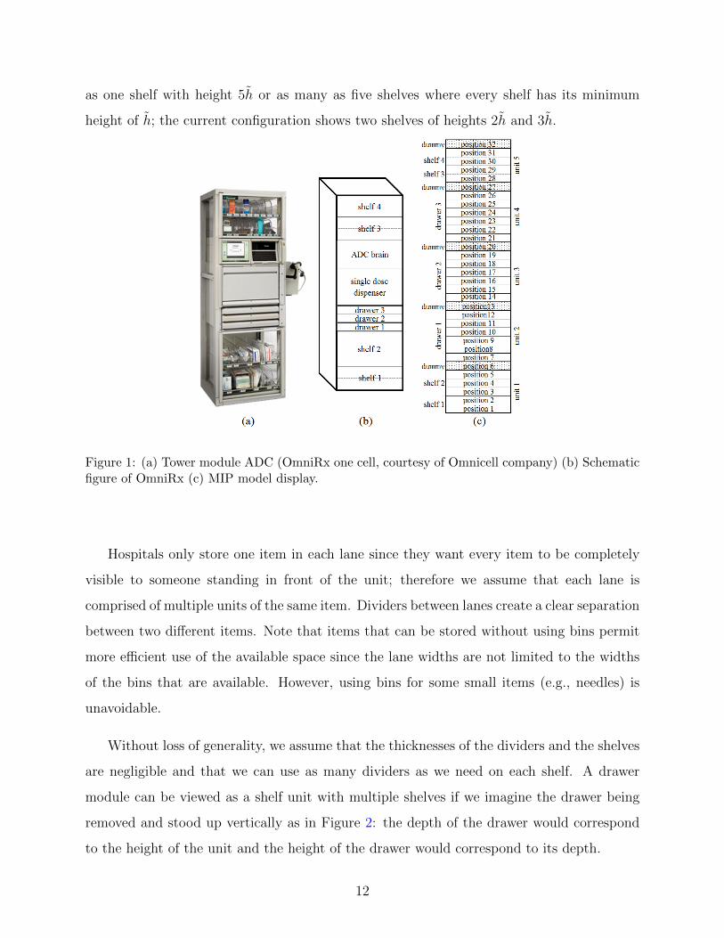
as one shelf with height 5h or as many as five shelves where every shelf has its minimum
height of h; the current configuration shows two shelves of heights 2h and 3h.
Figure 1: (a) Tower module ADC (OmniRx one cell, courtesy of Omnicell company) (b) Schematicfigure of OmniRx (c) MIP model display.
Hospitals only store one item in each lane since they want every item to be completely
visible to someone standing in front of the unit; therefore we assume that each lane is
comprised of multiple units of the same item. Dividers between lanes create a clear separation
between two different items. Note that items that can be stored without using bins permit
more efficient use of the available space since the lane widths are not limited to the widths
of the bins that are available. However, using bins for some small items (e.g., needles) is
unavoidable.
Without loss of generality, we assume that the thicknesses of the dividers and the shelves
are negligible and that we can use as many dividers as we need on each shelf. A drawer
module can be viewed as a shelf unit with multiple shelves if we imagine the drawer being
removed and stood up vertically as in Figure 2: the depth of the drawer would correspond
to the height of the unit and the height of the drawer would correspond to its depth.
12

Figure 2: (a) 24 compartment matrix drawer (b) General MIP model display (c) MIP model displayconfiguration
Finally we look at general ADC configurations such as the one shown in Figure 1 (a)
that could be comprised of multiple drawer, shelf or specialty sections/units. We handle
such systems by sequentially inserting a storage unit corresponding to each shelf section
and a storage unit for each drawer. A dummy position with a single shelf of height h is
inserted between different storage units. Our model ensures that nothing can be stored in
the dummy positions, which keeps each unit within the ADC distinct. When the “brain” is
an integral part of the cabinet or there are positions where items cannot be stored, these are
dropped altogether from the cabinet, and a dummy position is used to separate the storage
units above and below. We assume without loss of generality that each shelf unit and each
drawer “shelf” have the same minimum shelf height of h. Figure 1 (c) shows the schematic
representation of the cabinet shown in Figure 1 (a). Note that this cabinet has 2 shelf units
of heights 4h and 5h, and 3 drawer units each of “height” 6h. There are 5 dummy positions,
one at the top of each of the 5 storage units (we insert the dummy position at the top of the
upper-most unit for consistency and in case we have multiple cabinets). The overall height
of this cabinet is redefined to be (5 + 1 + 6 + 1 + 6 + 1 + 6 + 1 + 4 + 1)h = 32h units. Given
an ADC with K distinct storage sections (units) where unit c has height Hc, note that the
maximum possible number of shelf positions is M =∑C
c=1
⌊Hc
h
⌋+ C. In the remainder of
this chapter we will refer to all shelf heights in units of h.
We now provide the definition of a lane of item i on a shelf as follows:
Definition 1. A lane of item i is defined as a compartment on a shelf filled with at most ni
units of item i and has width wi, height hi, and depth D, where the height hi is the height
13

of item i in units of h, the width wi is either the width of item i or the width of the bin in
which it is stored, and D is the depth of the shelf. Units of an item are not stacked on top
of each other to fill the shelf space and the last lane of an item could be only partially filled
since filling it fully might cause the number of units of that item to exceed its upper bound.
Desired inventory values are commonly called “PAR levels” in hospital inventory man-
agement (Kelle et al. 2012); here PAR stands for Periodic Automatic Replenishment. A
common approach is to periodically review stock levels and reorder up to the PAR level
for each item. In the context of an ADC it is common to specify both a minimum and a
maximum PAR level (say, li and ui, respectively for an item i). We assume that an (s, S)
policy is used to manage ADC inventory, where s for an item i is set to the minimum PAR
level li and S can be freely chosen as long as it does not exceed the maximum PAR level ui.
The formulary is another important factor in pharmaceutical management on a patient
floor. A formulary refers to product variety and is a list of all medicines that might be
prescribed by physicians on a patient floor. Medication types and their max/min levels
within an ADC often require modifications over time due to changes in the composition of
the formulary level and dynamic demand characteristics (e.g., flu season, changes in drug
popularity). Given the limits on an ADC’s storage capacity, it cannot always contain all
patient care items, and regular assessments and periodic adjustments in its layout are needed.
In summary, we assume that at any given time there is a pool of items to choose from (the
formulary) along with a maximum and minimum PAR level for each. If an item is chosen
for storage in the ADC, the number of units stored must be at least its minimum PAR level.
However, we can choose the order-up-to level S based on the desirability of stocking the item
and to make efficient use of the limited storage space available, as long as this order-up-to
level S does not exceed the maximum PAR level.
Demand for items at the unit level differs by item, and item demands (Di) are in-
dependent random variables. Let the cumulative distribution function of Di be given by
Fi(d) = Pr(Di ≤ d). Our main goal is to pack a set of items into an ADC such that we
maximize the “value” of the set of items. The value of an item is defined in terms of the
14
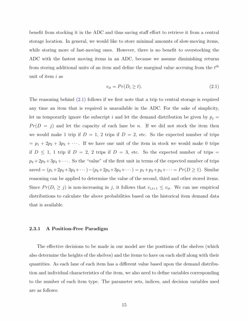
benefit from stocking it in the ADC and thus saving staff effort to retrieve it from a central
storage location. In general, we would like to store minimal amounts of slow-moving items,
while storing more of fast-moving ones. However, there is no benefit to overstocking the
ADC with the fastest moving items in an ADC, because we assume diminishing returns
from storing additional units of an item and define the marginal value accruing from the tth
unit of item i as
vit = Pr(Di ≥ t). (2.1)
The reasoning behind (2.1) follows if we first note that a trip to central storage is required
any time an item that is required is unavailable in the ADC. For the sake of simplicity,
let us temporarily ignore the subscript i and let the demand distribution be given by pj =
Pr(D = j) and let the capacity of each lane be n. If we did not stock the item then
we would make 1 trip if D = 1, 2 trips if D = 2, etc. So the expected number of trips
= p1 + 2p2 + 3p3 + · · · . If we have one unit of the item in stock we would make 0 trips
if D ≤ 1, 1 trip if D = 2, 2 trips if D = 3, etc. So the expected number of trips =
p2 + 2p3 + 3p4 + · · · . So the “value” of the first unit in terms of the expected number of trips
saved = (p1 +2p2 +3p3 +· · · )−(p2 +2p3 +3p4 +· · · ) = p1 +p2 +p3 +· · · = Pr(D ≥ 1). Similar
reasoning can be applied to determine the value of the second, third and other stored items.
Since Pr(Di ≥ j) is non-increasing in j, it follows that vi,t+1 ≤ vit. We can use empirical
distributions to calculate the above probabilities based on the historical item demand data
that is available.
2.3.1 A Position-Free Paradigm
The effective decisions to be made in our model are the positions of the shelves (which
also determine the heights of the shelves) and the items to have on each shelf along with their
quantities. As each lane of each item has a different value based upon the demand distribu-
tion and individual characteristics of the item, we also need to define variables corresponding
to the number of each item type. The parameter sets, indices, and decision variables used
are as follows:
15
Parameters
N : number of item types to store in the ADC
C: number of separate storage units in the ADC
Hc: height of section c ∈ {1, · · · , C}
M : maximum number of shelves possible in the ADC (i.e., M =∑C
c=1
⌊Hc
h
⌋+ C)
W : width of the ADC
vit: the marginal value of the tth unit of item i (as determined by equation (2.1))
ni: maximum number of item i that can be stored in one lane
li: minimum required number of item i if it is stored in the ADC
ui: maximum number of item i allowed to be stored in the ADC
wi: width of one lane of item i
hi: height of item i (in units of h)
ηc: maximum number of shelves possible in section c ∈ {1, · · · , C} i.e.,⌊Hc
h
⌋mi: maximum number of lanes of item i on one shelf, mi = min{
⌊Wwi
⌋,⌈uini
⌉}
Sets and Indices
I: index set of item types, i.e., I = {1, · · · , N}
H: index set of possible (vertical) shelf positions, i.e., H = {1, · · · ,M}
Hc: index set of possible (vertical) shelf positions in section c
H ′: index set of dummy (vertical) shelf positions
Si: index set of possible shelf positions along the height of the ADC for (a lane of) item i,
Ts: index set of possible items that can be stored on a shelf in vertical position s,
Li: the index set {1, · · · , ui}
Decision Variables
xis: number of lanes of item i located on shelf s (integer)
qi: = 1 if item i is stored in the ADC; 0 otherwise (binary)
zit: = 1 if there are at least t units of item i stored in the ADC; 0 otherwise (binary)
ys: = 1 if a shelf is located at position s; 0 otherwise (binary)
Note that there is a dummy position above each storage section so that H ′ = [η1 +
1, (η1 + η2) + 2, · · · ,∑c
j=1 ηc + c], and the index sets for shelves in the various sections are
16

given by H1 = {1, · · · , η1}, H2 = {η1 + 2, · · · , η1 + 1 + η2}, etc. Also note that Si =⋃Cc=1{c + (
∑c−1j=1 ηc), c + (
∑c−1j=1 ηc) + 1, · · · , c + (
∑cj=1 ηc) − hi} and we ensure that the top
most shelf location possible for item i in each section is such that there is sufficient height
to store it, while Ts (i.e., Ts = {i ∈ I : s ∈ Si}, where Ts ⊂ I) is the set of all items that
are not too tall for a shelf in position s. The idea behind defining these sets Si and Ts is to
reduce the number of integer and binary variables used in the formulations.
Model MIP1
max∑i∈I
∑t∈Li
vit zit, (2.2)
subject to:∑i∈Ts
wixis ≤ Wys ∀s ∈ H\H ′, (2.3)
∑t∈Li
zit ≤∑s∈Si
nixis ∀i ∈ I, (2.4)
liqi ≤∑t∈Li
zit ∀i ∈ I, (2.5)
miys + xir ≤ mi ∀s ∈ H\({1} ∪H ′),∀i ∈ Ts,∀r ∈ {max{1, s− hi + 1}, · · · , s− 1},
(2.6)
0 ≤ xis ≤ miqi, xis ∈ Z+ ∀i ∈ I, s ∈ Si, (2.7)
ys = 0, s ∈ H ′, ys ∈ {0, 1}, s ∈ H, (2.8)
zit ∈ {0, 1}, i ∈ I, t ∈ Li, qi ∈ {0, 1}, i ∈ I. (2.9)
The objective function (2.2) represents the total value across all lanes in the cabinet and
is the expected number of trips saved by a clinician not having to go to a central storage
location to retrieve a required item. Constraint set (2.3) ensures that the width constraint
for each shelf is satisfied. Constraint set (2.4) ensures that enough lanes are allocated for the
number of units of an item in the ADC and constraint set (2.5) ensures that if item i is stored
in the ADC then we store at least the minimum required number of that item. Constraint
set (2.6) ensures that no item on any lower shelf is tall enough to cause it to intrude into
the space occupied by the current shelf. Constraint set (2.7) ensures that if choose not to
17

stock an item in the ADC, no lanes are allocated for it and (2.8) ensures that we do not use
dummy shelves for storage.
Note that even though there might appear to be a large number of zit binary variables in
this formulation, we will prove (Proposition 1 in Section 2.4) that we can relax the integrality
of zit to simple lower and upper bounds of 0 and 1. Also, if the storage sections within an
ADC are not similar to each other (so that h varies by section), we can readily extend the
formulation by providing an additional subscript corresponding to each section c for h and
hi and slightly redefining ηc and Si as follows:
hc: minimum shelf height for section c
his: height of item i on shelf s ∈ Hc in units of hc
ηc: maximum number of shelves possible in section c ∈ {1, · · · , C} i.e.,⌊Hc
hc
⌋Si =
⋃Cc=1{c+ (
∑c−1j=1 ηc), c+ (
∑c−1j=1 ηc) + 1, · · · , c+ (
∑c−1j=1 ηc) + (ηc − his)}
2.3.2 A Position-Based Paradigm
We now propose a position-based model that addresses dispensing errors by selecting
and maintaining proper ADC inventory and also selecting appropriate ADC layouts. The
term LASA (look-alike, sound-alike) is used to refer to medications that have names that
have spelling similarities and/or similar phonetics. The ISMP recommends that LASA items
should not be stored next to each other. In addition, the FDA has published guidelines for
safety considerations with container labels and carton labeling designed to minimize medica-
tion errors. We integrate the ISMP and FDA information to determine potential interactions
between each pair of medications. Based on the literature and our data characteristics, we
define error coefficients based on medication categorical data, which may include LASA or
same medication names, package size and types (i.e., bottle, vial, box, ampule, etc), strength
and strength unit (mg, ml, gm, unit-dose, packet), form (tablet, capsule, liquid, powder, sup-
pository, patch, etc), and demand frequency (low, medium, high).
The error coefficient, eij, is defined for medication pair (i,j) based on the number of
factors in common relative to the maximum number of factors that are considered. A coef-
18

ficient value of 0 indicates that the medication pair has extremely dissimilar characteristics,
whereas a value closer to 1 indicates that the medication pair has very similar characteristics
and the items should not be located near one another. We define two thresholds for error
coefficients. We assume that if the error coefficient of a medication pair is greater than or
equal to ε (0 ≤ ε ≤ 1), they should not be stored next to each other on the same shelf and
at least one other item should be between them. If the error coefficient is greater than or
equal to ε′ (ε ≤ ε′ ≤ 1), they should not be stored on two consecutive shelves. The values of
ε and ε′ are decided by clinicians or other key hospital stakeholders.
It is important to note that each of the factors affecting the similarity of two items does
not have the same effect on the likelihood of inducing a picking error. For example, if a pair
of medications has LASA names then the chance of error is more than having just similar
package types or form. Therefore, in calculating an error coefficient between items i and
j, we assign a weight ωk to factor k, where the values of the weights are assigned by an
appropriately qualified individual. Suppose that there is a set K of factors that are relevant
when contrasting two items i and j. Suppose also that two items i and j are similar with
respect to some subset K ′ of these factors. Then the error coefficient between items i and j
can be computed as
eij =
∑k∈K′ ωk∑k∈K ωk
, (2.10)
To solve this second model more efficiently, we do some preprocessing to reduce the
number of binary variables required. We start by estimating the maximum number of lanes
we could have on a shelf, given that a single lane with some item i ∈ I has been assigned
to it. Let us denote this number by γmaxi for item i. To compute this value for a given i
we first sort all of the items in increasing order of their lane widths (with ties being broken
arbitrarily), along with corresponding estimates of the maximum number of lanes possible
in the cabinet for each item (=⌈ujnj
⌉for item j). To the existing lane of item i we then
start adding additional lanes starting at the top of this list (i.e., with the item having the
smallest lane width) one at a time, until we reach the upper limit on its number of lanes (at
which point, we move on to the next item on the list), or until adding the next lane would
cause us to exceed the width of the cabinet (W ); the corresponding number of lanes at that
19

point gives us the value of γmaxi . The sets, indices, parameters and decision variables that
are needed in addition to the ones already defined in Section 2.3.1 are as follows:
Parameters
eij: error coefficient between item i and j, 0 ≤ eij ≤ 1
ε: the maximum allowable error coefficient between two items stored next to each other on
the same shelf
ε′: the maximum allowable error coefficient between two items stored on two adjacent shelves
Sets and Indices
γi: index set of possible positions along a shelf for item i starting at the left, i.e., {1, · · · , γmaxi }
Λ: the index set {1, · · · ,maxi γmaxi }
∆l: set of possible items for horizontal position l, ∆l = {i ∈ I : l ∈ γi}, where ∆l ⊂ I
Decision Variables
xisl: = 1 if a lane of item i is located on shelf s in horizontal position l; 0 otherwise (binary)
Note that we number horizontal positions consecutively starting from the left end of the
shelf. How many such positions exist depends upon what items we store on the shelf; the
set γi indexes these positions (up to a maximum of γmaxi ) when we are given that one of
those positions is occupied by item i. The set ∆l ensures that we do not consider item i for
a position l if that position is not feasible for item i on the shelf. In general, the set ∆l will
only be limited for larger values of l, i.e., on the right side of the ADC.
20

Model MIP2
max∑i∈I
∑t∈Li
vit zit, (2.11)
subject to:∑i∈Ts
∑l∈γi
wixisl ≤ W ∀s ∈ H\H ′, (2.12)
∑i∈(Ts∩∆l)
xisl ≤ 1 s ∈ H\H ′, l ∈ Λ, (2.13)
xisl + xjrk ≤ 1 ∀i, ∀s ∈ Si,∀l ∈ γi,∀r ∈ {s+ 1, · · · , s+ hi − 1},∀j ∈ Tr,∀k ∈ γj,
(2.14)
xisl + xjsk −∑i′ 6=i,j
k−1∑l′=l+1
xi′sl′ ≤ 1 ∀s,∀i, j ∈ Ts 3 i 6= j, eij ≥ ε,∀l ∈ γi, k ∈ γj,
(2.15)
xisl + xjs+hik ≤ 1 ∀r 3 s, s+ hk ∈ Hr,∀i ∈ Ts, ∀j ∈ Ts+hi (2.16)
3 i 6= j, eij ≥ ε′,∀l ∈ γi, k ∈ γj (2.17)∑t∈Li
zit ≤∑s∈Si
∑l∈γi
nixisl ∀i ∈ I, (2.18)
liqi ≤∑t∈Li
zit ∀i ∈ I, (2.19)
xisl ≤ qi i ∈ I, s ∈ Si, l ∈ γi, xisl ∈ {0, 1} i ∈ I, s ∈ Si, l ∈ γi, (2.20)
zit ∈ {0, 1}, i ∈ I, t ∈ Li, qi ∈ {0, 1}, i ∈ I. (2.21)
The objective function (2.11) and constraint set (2.12) are similar to (2.2) and (2.3), respec-
tively. Constraint set (2.13) ensures that every horizontal position along a shelf is assigned
to a lane for at most one item. Constraint set (2.14) ensures that the height of a shelf is
determined by the height of the tallest item by ensuring that there is no shelf that would be
“running through” an item on the current shelf. Constraint set (2.15) prevents two items
i and j with an error coefficient more than ε from being next to each other on the same
shelf by ensuring that there is at least one other item in between these two items, while
(2.17) prevents two items with an error coefficient more than ε′ from being stored on adja-
cent shelves unless there is intervening empty space above the item in the lower shelf that
21
separates the two items. Constraint sets (2.18), (2.19) and (2.20) are similar to (2.4), (2.5)
and (2.7), respectively.
2.4 TIGHTENING AND ENHANCING THE MIP FORMULATIONS
In this section, we present several enhancements in the form of valid inequalities and re-
laxations for the models in Section 2.3 in order to improve their computational performance.
Later, in Section 2.5 we will discuss the efficacy of these enhancements using several test
instances.
Symmetries constitute one of the main problems when dealing with exact methods for
discrete optimization. Numerous authors have noted the importance of resolving this issue
when solving MIPs for combinatorial problems (e.g., Sherali and Smith (2001)). Formulations
of packing and layout problems in particular can result in considerable degeneracy due to
symmetry and redundant sequences. Removing such alternatives from a model can lead
to a dramatic reduction in computational effort because considerable effort is expended in
evaluating each of these. We address this issue through the addition of valid inequalities
using the theorems of this section.
In our first model, some symmetries are avoided since we do not need to explicitly
distinguish the position of an item on a shelf. However, the model does decide where a shelf
is positioned within the cabinet, and therefore, one of the symmetries to be resolved arises
from the permutations of shelves. We propose a class of valid inequalities in Theorem 1
that sorts the shelves from the tallest to the shortest, starting at the bottom. These valid
inequalities are defined separately for each storage section c of an ADC.
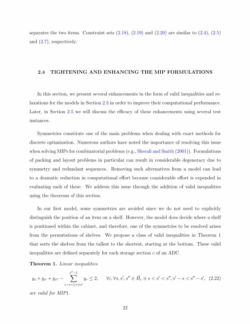
Theorem 1. Linear inequalities
ys + ys′ + ys′′ −s′′−1∑
r=s+1,r 6=s′yr ≤ 2, ∀c, ∀s, s′, s′′ ∈ Hc 3 s < s′ < s′′, s′ − s < s′′ − s′, (2.22)
are valid for MIP1.
22
Proof. Suppose that an optimal solution of MIP1 violates one of the inequalities in (2.22),
say for s = a, s′ = b, s′′ = c. This implies that there are three consecutive shelves at
positions a, b and c and the shelf at a higher location b is taller (s′′ − s′) than the shelf
below it at location a (s′− s). However, it is always possible to swap the order of shelves at
locations a and b by moving the shelf at position b (along with its contents) to position a,
and moving the shelf at position a (along with its contents) to position a + (c− b) without
altering any other aspect of the optimal solution. Therefore these inequalities are valid for
MIP1.
Another issue that is unique to the problem that we consider is the fact that several
items that are stored in ADCs have very similar size and demand, and therefore contribute
the same or similar amounts to the objective for the first model while consuming the same or
similar amounts of space. For example, based on actual data, we have observed that different
concentrations of the same medication often have the same size and similar demand. This
can cause our model to expend considerable effort in choosing between items that are the
same or very similar when limited space is to be assigned to one (or a subset) of such items.
To address this we first introduce the following definition.
Definition 2. ψik =∑min{kni,ui}
t=(k−1)ni+1 vit
To interpret this definition, the quantity kni represents the total number of units of item
i in the ADC if we fill k lanes with units of this item. Note that once we decide to store an
item, there is no reason to not fill the last lane entirely, unless doing so exceeds the upper
bound (ui) on the number of units allowed. This is true because by doing so the objective
function can be improved while none of the constraints are affected. Then ψik represents the
value of the total number of units of item i that we can store in lane k.
In a preprocessing step, we first index our items in decreasing order of their heights,
breaking ties arbitrarily. The following theorem proposes a class of valid inequalities that
removes dominated cases by choosing one item over another when it takes up less space while
also adding more value. These inequalities also breaks ties in those cases where two items
23
require the same amount of space and have the same demand, based on our indexing scheme.
Also, for notational convenience, let us refer to⌈lini
⌉and
⌈uini
⌉as Li and Ui, respectively.
Note that Li and Ui represent the number of lanes needed to store the minimum required
and maximum allowable amounts (li and ui, respectively) of an item i selected for storage.
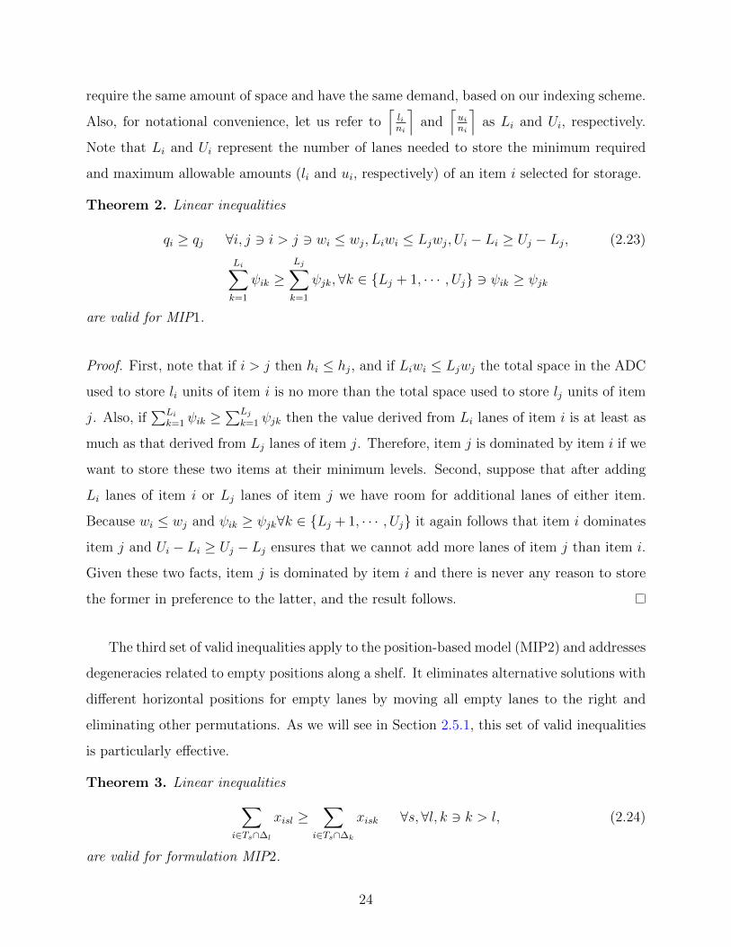
Theorem 2. Linear inequalities
qi ≥ qj ∀i, j 3 i > j 3 wi ≤ wj, Liwi ≤ Ljwj, Ui − Li ≥ Uj − Lj, (2.23)
Li∑k=1
ψik ≥Lj∑k=1
ψjk,∀k ∈ {Lj + 1, · · · , Uj} 3 ψik ≥ ψjk
are valid for MIP1.
Proof. First, note that if i > j then hi ≤ hj, and if Liwi ≤ Ljwj the total space in the ADC
used to store li units of item i is no more than the total space used to store lj units of item
j. Also, if∑Li
k=1 ψik ≥∑Lj
k=1 ψjk then the value derived from Li lanes of item i is at least as
much as that derived from Lj lanes of item j. Therefore, item j is dominated by item i if we
want to store these two items at their minimum levels. Second, suppose that after adding
Li lanes of item i or Lj lanes of item j we have room for additional lanes of either item.
Because wi ≤ wj and ψik ≥ ψjk∀k ∈ {Lj + 1, · · · , Uj} it again follows that item i dominates
item j and Ui − Li ≥ Uj − Lj ensures that we cannot add more lanes of item j than item i.
Given these two facts, item j is dominated by item i and there is never any reason to store
the former in preference to the latter, and the result follows.
The third set of valid inequalities apply to the position-based model (MIP2) and addresses
degeneracies related to empty positions along a shelf. It eliminates alternative solutions with
different horizontal positions for empty lanes by moving all empty lanes to the right and
eliminating other permutations. As we will see in Section 2.5.1, this set of valid inequalities
is particularly effective.
Theorem 3. Linear inequalities∑i∈Ts∩∆l
xisl ≥∑
i∈Ts∩∆k
xisk ∀s,∀l, k 3 k > l, (2.24)
are valid for formulation MIP2.
24
Proof. Suppose that in an optimal solution of MIP2, an inequality in (2.24) is violated for
some particular l, k. This implies that position l is empty but a position k to its right is
occupied. However, we can shift all items in positions l + 1 through k one position to the
left and move the empty space to position k to obtain an equivalent optimal solution such
that all inequalities (2.24) are satisfied. The result follows.
When we use inequality set (2.24), we can replace (2.15) with the following constraint
set, because all of the empty shelves has been pushed to the right side of the shelf; this
results in a smaller number of constraints as well as a sparser coefficient matrix:
xisl + xjs,l+1 ≤ 1 ∀s,∀i, j ∈ Ts 3 i 6= j, eij ≥ ε,∀l ∈ γi, l + 1 ∈ γj (2.25)
Another way to enhance computational performance is to relax the integrality restriction
on binary variables that are guaranteed to be either 0 or 1 at the optimum. In our formula-
tions, a critical result is that we can replace the binary restrictions for zit with 0 ≤ zit ≤ 1.
The following proposition shows that this relaxation is valid as long as vit is strictly positive.
Proposition 1. There exist optimal solutions (x∗,y∗, q∗, z∗) to model MIP1 and (x∗, q∗, z∗)
of model MIP2 with the relaxations 0 ≤ z ≤ 1, with all elements of the vector z∗ havig binary
values.
Proof. Suppose we have an optimal solution (x∗,y∗, q∗, z) with fractional values for elements
of z in model MIP1 with the z variables relaxed. The two constraints that are relevant are
(2.4) and (2.5). Note that the LHS of (2.4) and (2.5) are both integers. For notational ease,
let us use Qi to denote the integer∑
s∈Sinix
∗is, so that (2.4) and (2.5) reduce to
liqi ≤∑t∈Li
zit ≤ Qi (2.26)
25

Case 1: Qi ≥ ui
Define z∗it = 1 for all t ∈ Li, i.e., t = 1, · · · , ui. This satisfies (2.26) since∑
t∈Liz∗it = ui.
Also, since zit ≤ z∗it for all t it follows that∑
t∈Livitzit ≤
∑t∈Li
vitz∗it =
∑t∈Li
vit and since
z is optimal it follows that it cannot have any fractional components.
Case 2: li ≤ Qi < ui
Define z∗it = 1 for t = 1, 2, · · · , Qi, and z∗it = 0 for t = Qi + 1, Qi + 2, · · · , ui. Again, it is
clear that z∗ satisfies (2.26) and item i contributes∑Qi
t=1 vitz∗it =
∑Qi
t=1 vit to the objective
function. So this is a lower bound to the contribution from item i to the objective with
the vector z. Now, with the vector z, item i contributes∑Qi
t=1 vitzit +∑ui
t=Qi+1 vitzit to the
objective. Consider zit for t ≤ Qi; if all these values are 1 then we cannot have zit positive for
any t > Qi (otherwise (2.26) would be violated). So zit for some t ≤ Qi has to be fractional.
Consequently, at least one zit > 0 for some t > Qi because otherwise the contribution of item
i to the objective would be smaller than the lower bound of∑Qi
t=1 vit and thus the vector z
could not be optimal. We could then reduce zit for one or more of these values of t > Qi and
increase the (fractional) value for t ≤ Qi by the same amount and obtain a solution that is
at least as good, since vit is non-increasing in t. Since the most that we could increase any
value of zit for each t ≤ Qi is to the point where each of them is equal to 1 (at which point
every zit for t > Qi must be zero) the upper bound on the contribution we can get from
item i in the optimal objective is∑Qi
t=1 vit. Thus the vector with z∗it as defined above must
be optimal.
The proof for Model MIP2 is similar and is omitted. In general, this proposition tells us
that we can solve the relaxation and we will either obtain a binary solution (case 1) or if we
obtain a fractional z vector we can use the x vector to redefine a new binary z vector that
yields the same optimum value.
26

2.5 COMPUTATIONAL ANALYSIS
In this section, we illustrate our models using numerical examples based on real data
derived from drawer module ADC transactions at ten ADC stations across multiple hospitals
within a healthcare system in Pennsylvania, each with several hundred beds. We name these
data sets PA1, · · · , PA10. Table 1 displays some information for each of the ten data sets:
the upper section shows statistical information about items, and the lower section displays
the number of unique medication pairs that are similar with respect to the pertinent factor
corresponding to that row.
The computations are all done using a standard solver (CPLEX 12.4) with up to eight
threads on three machines using the same hardware specifications (Intel Xeon Processor E5−
2690). We set the symmetry breaking parameter in CPLEX at the “extremely aggressive”
level since our model has many symmetries. In general, we impose a 10 hour run time limit
for the numerical examples, but for some of the harder problems thus increases this to 24
hours (all CPU times given in seconds).
We report results from three types of numerical studies. In Section 2.5.1, we evaluate the
relative effectiveness of the valid inequalities introduced in Section 2.4. In Section 2.5.2, we
do some benchmarking. First, we compare the performance of our approach with heuristic
techniques described in the literature that can be adapted to our problem and that represent
what might be commonly done in practice. We then also compare our simpler model (MIP1)
with one of the best MIP models in the literature for some limited cases where the latter
model can be adapted to our problem. Finally, in Section 2.5.3, we compare and contrast
MIP1 and MIP2.
2.5.1 Analysis of Valid Inequalities
While we can eliminate many of the redundancies resulting from symmetry by using the
valid inequalities presented in Sections 2.4, we have to balance this against the increase in
27

Table 1: ADC transaction data set characteristics and number of medication pairs based on differentsimilarity factors
Factors PA1 PA2 PA3 PA4 PA5 PA6 PA7 PA8 PA9 PA10
no. of item types 105 98 97 127 111 104 125 86 93 90
max. no. of items 1333 1483 887 1100 975 915 1101 902 954 834
mean demand 11.6 13.2 7.57 8.90 8.91 7.27 9.43 8.83 9.03 9.31
mean size (in3) 60.1 60.7 104.0 91.8 90.0 97.3 84.9 48.9 69.2 67.4
name 86 83 51 59 52 54 43 71 60 41
unit 2170 2266 1950 2405 1881 2380 1659 2294 1882 1627
dosage 850 535 1002 890 800 1270 863 942 722 580
package 371 221 436 382 298 563 308 407 296 227
strength & unit 142 159 132 188 112 162 149 148 148 98
the number of constraints, which in general can cause the run time to increase. We consider
a single and double column tower module ADC (Pyxis Medstation ES) where each column
has size 79.5 × 31.0 × 28.0 in3 (i.e., H ×W ×D) with at most 18 shelves of height 4.4 in.
We compare the base version of model MIP1 with versions that have different combinations
of the valid inequalities defined by (2.22) and (2.23) for both column configurations of the
ADC.
The charts in Figures 3 and 4 provide a graphical view of the results for the single and
double column configurations, respectively. The three bars on each chart for a given problem
correspond to the cases with (a) inequality set (2.22), (b) inequality set (2.23) and (c) both
sets of valid inequalities. When the problem could be solved using the base model we plot
the value of time for versiontime for base model
, i.e., the version’s run time as a fraction of the base model’s run
time. In cases where the problem could not be solved by the base model we plot the value
of time for versionallowed time limit
if the version in question could solve the problem, and 1.0 otherwise.
28

Figure 3: ADC transaction data set characteristics and number of medication pairs based ondifferent similarity factors
For the problems where the version with both (2.22) and (2.23) took more than 5 hours,
we allowed the other versions to run for a maximum of 24 hours instead of 10 hours (e.g.,
PA3, PA4, PA5 and PA7 with the double column ADC). For instances where the base model
(without any valid inequalities) took under one minute, there is clearly no need for valid
inequalities and we do not study these further (e.g., PA8 and PA10 with the double column
ADC).
Figures 3 shows that for the single module ADC the reductions in run time from the
base model by using (2.22) and (2.23) are more than 90% in most cases. We also see that
inequality set (2.22) is more effective when the average size of items in our list is smaller
(PA1, PA8, PA9); inequality set (2.23) tends to be more effective when the average size
of items on our list is smaller and the demand is also higher (PA1, PA2); and using both
inequality sets (2.22) and (2.23) has the most effect when the number of item types increases
(PA4, PA6). Figure 4 indicates that problems with the double column ADC are harder to
solve because of the increased search space (larger feasible region), except when there is
enough room to store all items at their upper limit (e.g., PA8, PA9 and PA10), and that it
is not possible to solve our problems without having both sets of valid inequalities.
29

Figure 4: Runtime with different combinations of valid inequalities, as a fraction of runtime withoutvalid inequalities (double column ADC)
In summary, adding both classes of valid inequalities allows us to solve all of our problem
instances and also produces a significant reduction in run time. Of the eighteen instances
analyzed there were five that could be solved by the base version and across these five
instances, the average CPU time for the version with both valid inequalities is around 16%
of the base model’s time. For the remaining thirteen instances, the CPU time is at most 22%
of the base model’s time; the actual values are likely to be lower. The results from using the
valid inequalities defined by (2.24) along with MIP2 are similar. We tested the effectiveness
of these inequalities using instance PA1 with different combinations of ε and ε′ for different
ADC sizes. We choose ε and ε′ in such a way that a% of the item pairs are precluded from
being stored next to each other and b% of the pairs are precluded from being stored on
adjacent shelves, resulting in three combinations: (a, b) = {(0%, 0%), (25%, 0), (25%, 8%)}.
We also define the different ADC sizes as a function of the number of drawers, p, and the
number of compartments in each drawer, q, and explore combinations of p ∈ {1, 2, 3, 4, 5} and
q ∈ {6, 12, 24, 48}. Across all of the different ADC size combinations, the average reductions
in CPU time by using (2.24) for MIP2 for the (25%, 0) and (25%, 8%) cases are 94% and 76%,
respectively. Recall that this set of valid inequalities is related to permutations of items on
shelves, and therefore, when we have restrictions only on the shelves (i.e., case (25%, 0%)),
30
the effectiveness of this set of valid inequalities is more evident. Detailed results are shown
in Table 2. For larger instances with 12 or more compartments per drawer, the base MIP2
model was not able to obtain solutions within the ten hour limit when at least one of either
ε and ε′ is not zero, while using the valid inequalities enabled all problems to be solved.
2.5.2 Benchmarking
In this section, we compare the results from our model with those obtained by adapting
some common heuristic procedures that might be plausibly implemented in practice, and
also with an efficient 2TDK IP model from the literature. Note that there are sophisticated
heuristics for shelf-space allocation that could be adapted to our problem, but due to the
complexity of their implementation these could take just as much (or more) effort than using
our model. In order to estimate the likely real benefits of our approach, we therefore chose
to compare it with the heuristics in Jylanki (2010) that are similar to the simple rules used
in practice . Each method represents a combination of a sequencing rule to determine which
item to select next, and a greedy heuristic to determine how to allocates items to shelves.
The general approach is as follows:
1. Sequencing: Choose one of the following ranking rules to obtain a sorted list of items (in
all cases, ties are broken arbitrarily).
− R1: non-increasing order of item value of the first unit of the item, i.e., vi1
− R2: non-increasing order of the value of the first lane of an item, i.e.,∑
t∈{1,··· ,ni} vit
− R3: non-increasing order of the value of the first unit of its lane surface area, i.e., vi1hiwi
− R4: non-decreasing order of lane height, i.e., hi
− R5: non-decreasing order of lane volume, i.e., hi × wi × di2. Heuristic selection: Choose a space allocation heuristic from the following:
− Shelf First Fit (SFF): store items in the first feasible location starting from the first
shelf
− Shelf Best Width Fit (SBWF): store items to minimize unused width
− Shelf Best Height Fit (SBHF): store items to minimize unused height
31

Table 2: Summary of valid inequalities effects for Model MIP2 considering different percentages ofnonadjacent medication pairs on and between shelves
(a,b)=(0%,0%) (a,b)=(23%,0%) (a,b)=(23%,8%)
# p(q)CPU seconds CPU seconds CPU seconds
MIP2 MIP2+VI MIP2 MIP2+VI MIP2 MIP2+VI
1 1(6) 2.529 1.763 10.34 2.200 13.40 5.398
2 2(6) 3.480 2.512 49.51 4.493 31.86 8.362
3 3(6) 4.512 3.198 67.02 7.738 1,097 882.3
4 4(6) 4.791 3.869 313.5 9.376 14,000 950.7
5 5(6) 6.165 5.507 590.7 15.62 584.8 224.4
6 1(12) 3.151 3.026 597.5 62.59 1,138 87.50
7 2(12) 4.181 4.134 * 1,051 * 27,156
8 3(12) 9.422 5.990 * 62.23 * 1,556
9 4(12) 10.45 7.847 * 128.4 * 411.8
10 5(12) 15.10 9.656 * 192.3 * 3,601
11 1(24) 4.087 3.931 * 7,201 * 3,916
12 2(24) 10.14 9.188 * 232.5 * 296.6
13 3(24) 17.74 16.49 * 179.2 * 1,851
14 4(24) 25.59 23.24 * 673.1 * 570.8
15 5(24) 15.77 14.20 3557.65 68.19 * 279.8
16 1(48) 34.43 11.70 * 1,505 * 33,983
17 2(48) 114.9 32.00 * 731.1 * 1,136
18 3(48) 189.4 56.49 * 1,893 * 20,688
19 4(48) 158.0 48.20 * 1,882 * 2,939
20 5(48) 115.5 41.50 * 236.2 * 834.9
*: after 10 hours, the code was still running
32

− Shelf Best Area Fit (SBAF): store items to minimize unused surface area
3. Initial allocation: Allocate items to their minimum levels starting with the first item on
the list; if there is not enough space to store an item at its minimum level, then don’t store
that item at all and go to the next item. Continue until the end of the list is reached.
4. Final allocation: If there is space still available on one or more shelves, choose sequentially
from items already stored (at their minimum levels) and try to store additional units up to
the item’s maximum level using the heuristic selected in step 2. If there is not enough space
available to store the item to its upper limit, store as much as possible and go on to the next
item.
We ran all combinations of sequencing rules and heuristics for all ten data sets. For all
problems we computed the ratio of the solution obtained and the optimum solution. These
were then averaged across all ten test problems and the results are shown in the left half of
Table 3. The right half of Table 3 shows the ratio of the space utilization for the heuristic
versus that of the optimal solution (again, averaged across the ten test problems). It is clear
that none of the heuristics are particularly efficient. In general, the combination of SFF
and R5 appear to the best. On average, across all cases considered and across all ten data
sets (200 instances), the objective value and space utilization with the heuristics are 50%
and 82% of the corresponding optimum values, which suggests that simplistic methods could
result in about twice as much work for medical staff while still leaving unused space in the
ADC.
We also contrast model MIP1 with that of Lodi and Monaci (2003), which is considered
to be the best polynomial size model in the 2TDK literature (Furini and Malaguti (2013));
henceforth, we will refer to their model as the LM Model. The LM model is directly adaptable
to our problem only for the specific case where we have a single, continuous storage section
in the ADC (an example might be the the tower module Pyxis MedStation ES). In such
instances, the section might be viewed as a single “sheet” from which pieces are to be cut
out using guillotine cuts. The corresponding adaptation to our problem may be found in
the Appendix. We perform the comparison for various sizes of the tower module ADC
considered, resulting in 28 different test instances. To benchmark the performance of MIP1
33
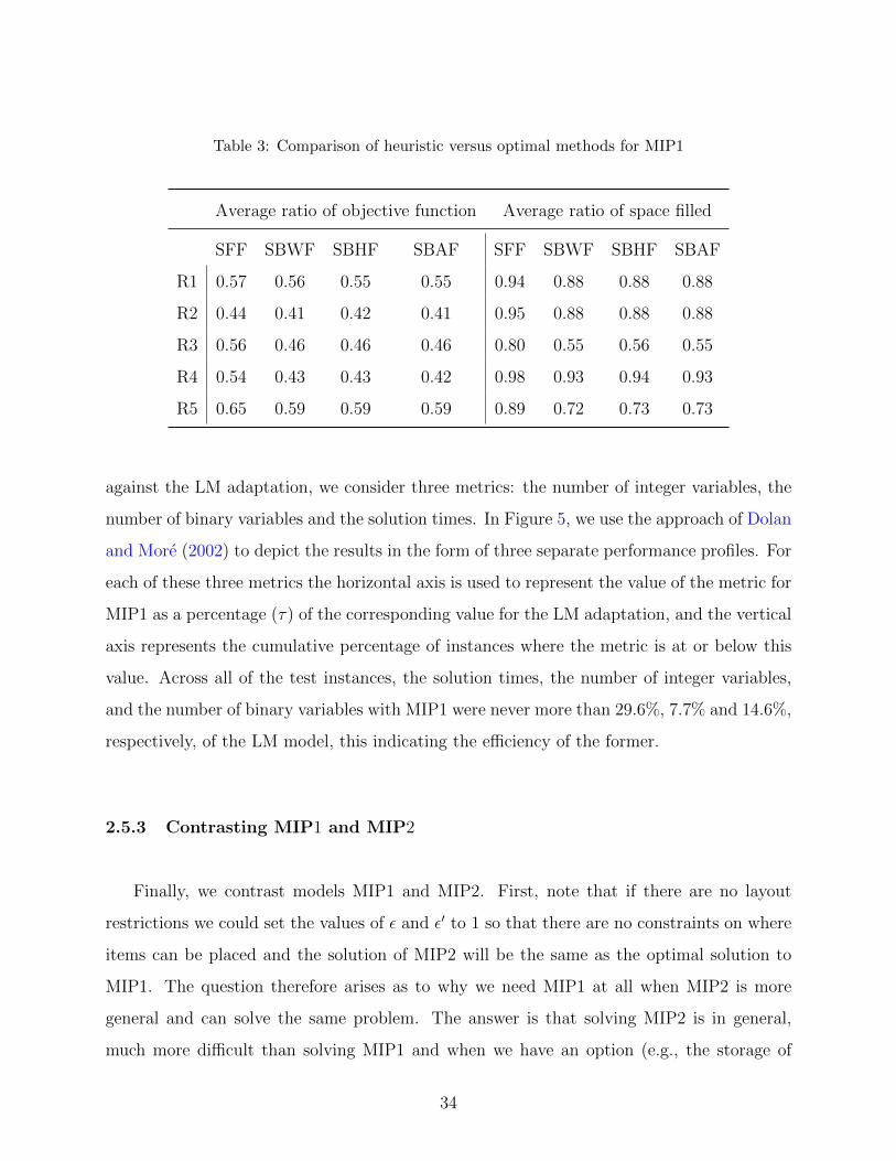
Table 3: Comparison of heuristic versus optimal methods for MIP1
Average ratio of objective function Average ratio of space filled
SFF SBWF SBHF SBAF SFF SBWF SBHF SBAF
R1 0.57 0.56 0.55 0.55 0.94 0.88 0.88 0.88
R2 0.44 0.41 0.42 0.41 0.95 0.88 0.88 0.88
R3 0.56 0.46 0.46 0.46 0.80 0.55 0.56 0.55
R4 0.54 0.43 0.43 0.42 0.98 0.93 0.94 0.93
R5 0.65 0.59 0.59 0.59 0.89 0.72 0.73 0.73
against the LM adaptation, we consider three metrics: the number of integer variables, the
number of binary variables and the solution times. In Figure 5, we use the approach of Dolan
and More (2002) to depict the results in the form of three separate performance profiles. For
each of these three metrics the horizontal axis is used to represent the value of the metric for
MIP1 as a percentage (τ) of the corresponding value for the LM adaptation, and the vertical
axis represents the cumulative percentage of instances where the metric is at or below this
value. Across all of the test instances, the solution times, the number of integer variables,
and the number of binary variables with MIP1 were never more than 29.6%, 7.7% and 14.6%,
respectively, of the LM model, this indicating the efficiency of the former.
2.5.3 Contrasting MIP1 and MIP2
Finally, we contrast models MIP1 and MIP2. First, note that if there are no layout
restrictions we could set the values of ε and ε′ to 1 so that there are no constraints on where
items can be placed and the solution of MIP2 will be the same as the optimal solution to
MIP1. The question therefore arises as to why we need MIP1 at all when MIP2 is more
general and can solve the same problem. The answer is that solving MIP2 is in general,
much more difficult than solving MIP1 and when we have an option (e.g., the storage of
34

Figure 5: Performance profiles for MIP1 as percentages of those of the LM adaptation
hospital supplies where picking errors are not serious) it is definitely preferable to use the
simpler model. To compare the ease of solving the same problem via MIP1 and MIP2 (with
ε and ε′ set to 1), we consider two data sets (PA1 and PA10) and test both models along
with their valid inequalities for different ADC sizes such as p ∈ {1, 2, 3, 4, 5} drawers and
q ∈ {6, 12, 24, 48, 96} compartments per drawer. In all cases the run times for MIP1 are lower
than those for MIP2, with the average reduction in run time from MIP2 to MIP1 being 73%
and 81% for PA1 and PA10, respectively. More importantly, the relative effort required for
MIP2 starts to grow as the problems become larger (more storage compartments). For 9 of
the 50 instances tested the run time with MIP2 hits the ten-hour threshold. These results
indicate that if items being stored are not similar or if item-picking errors do not constitute
a significant issue, it is much more efficient to use the simpler MIP1 model.
Conversely, when the layout is critical we require MIP2. A question that might arise is
whether one could just use MIP1 for a problem while ignoring layout restrictions to easily
obtain the optimal value, and then manually find a layout that is feasible with respect to the
35

layout restrictions. Unfortunately, this is generally not a viable approach, and we do require
MIP2 for problems requiring layout consideration. We use a simple example to illustrate
this point. Consider the 10 different medications shown in Table 4 that have various degrees
of similarity; e.g., medication pairs (1, 3), (2, 3), (4, 9), (4, 10) and (7, 8) are LASA pairs
based on the ISMP and FDA lists. We choose K = 8 using factors such as name, dosage,
package type, strength, unit, demand, size, and the combination of strength and unit with
corresponding ωk values of 1.0, 0.2, 0.3, 0.2, 0.1, 0.1, 0.2, and 0.3 based on expert opinion.
Consider the relatively easy case where ε = 0.04 and ε′ = 1. We chose ε = 0.04 because this
is the smallest value for which MIP1 and MIP2 both yield the same optimal value. Suppose
that we attempt to manually configure the layout after solving MIP1. Figure 6 illustrates
(a) a layout that is randomly generated from the set of optimal solutions to MIP1, (b) an
improved layout obtained by manually rearranging items within the same shelf (shelves 1
and 4), (c) a further improvement obtained by exchanging items between shelves (shelves
1 and 3), and (d) the layout obtained from MIP2 (note that all have the same value for
the objective). The value of the sum of the error coefficients eij (which we call the layout
total error, LTE) for these four cases are 3.5, 2.37, 1.17 and 0.04, respectively. Note that
the changes in going from (a) to (b) are what one might typically expect from clinical staff,
while going from (b) to (c) would be far more difficult. Yet, even this is not satisfactory
compared to the layout from MIP2. This reinforces why MIP2 is essential in many cases.
To study the effectiveness of MIP2 in reducing LTE versus MIP1, we run numerical results
for all ten data sets, i.e., PA1, PA2, · · · , PA10, and for ten ADC sizes, i.e., p ∈ {1, · · · , 5},
and q ∈ {6, 12}. We chose ε in a way that an average of approximately 18% of the item
pairs are prohibited from being stored next to each other and the optimal objective function
value remains the same in both MIP1 and MIP2. When compared to a layout randomly
selected from the set of optimal solutions of MIP1, the average reduction in the LTE value
from MIP2 across the 100 problems tested was approximately 38%. Thus MIP2 can be used
to significantly reduce the likelihood of picking errors.
36
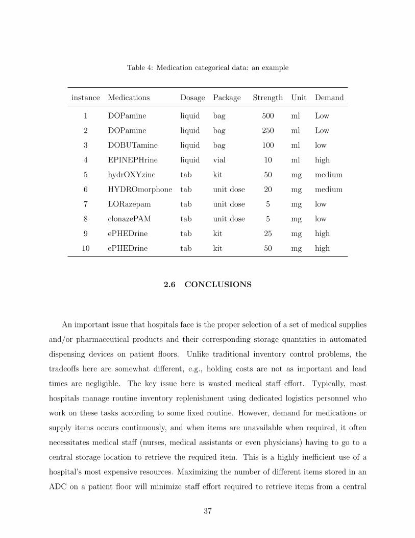
Table 4: Medication categorical data: an example
instance Medications Dosage Package Strength Unit Demand
1 DOPamine liquid bag 500 ml Low
2 DOPamine liquid bag 250 ml Low
3 DOBUTamine liquid bag 100 ml low
4 EPINEPHrine liquid vial 10 ml high
5 hydrOXYzine tab kit 50 mg medium
6 HYDROmorphone tab unit dose 20 mg medium
7 LORazepam tab unit dose 5 mg low
8 clonazePAM tab unit dose 5 mg low
9 ePHEDrine tab kit 25 mg high
10 ePHEDrine tab kit 50 mg high
2.6 CONCLUSIONS
An important issue that hospitals face is the proper selection of a set of medical supplies
and/or pharmaceutical products and their corresponding storage quantities in automated
dispensing devices on patient floors. Unlike traditional inventory control problems, the
tradeoffs here are somewhat different, e.g., holding costs are not as important and lead
times are negligible. The key issue here is wasted medical staff effort. Typically, most
hospitals manage routine inventory replenishment using dedicated logistics personnel who
work on these tasks according to some fixed routine. However, demand for medications or
supply items occurs continuously, and when items are unavailable when required, it often
necessitates medical staff (nurses, medical assistants or even physicians) having to go to a
central storage location to retrieve the required item. This is a highly inefficient use of a
hospital’s most expensive resources. Maximizing the number of different items stored in an
ADC on a patient floor will minimize staff effort required to retrieve items from a central
37

Figure 6: (a) A layout from MIP1 (LTE=3.5), (b) Layout after initial reordering (LTE=2.37), (c)Layout after further reordering (LTE=1.17), (d) Layout from MIP2 (LTE=0.04)
pharmacy/storage location when they are unavailable. However, the total storage space in
an ADC is constrained and units of different items take up different amounts of the available
space. In addition, the demand characteristics of items are different and also vary by location
within the hospital. One must consider all of these factors when selecting the right set of
items for storage. A related issue that is often just as important is the layout of the selected
items within storage, given that there is flexibility in how an ADC is configured. This is
especially true with storage of pharmaceutical supplies when picking errors can have very
serious consequences. In this case one must also determine how items are actually distributed
among the shelves or compartments of a cabinet. It is also worth mentioning that hospitals
update the items stored on patient floors approximately once every three months and thus
these questions might need to be answered on an ongoing basis.
We address all these issues with two different MIP models. In both models the objective
is to minimize the expected staff effort to retrieve items that are unavailable when required.
The first model uses what we refer to as a position-free paradigm. It is simpler and easier
to solve and can be used when the layout of items within the ADC is not critical (e.g.,
with routine medical supplies). This model determines what items to store and how many
units of each, along with the overall shelf configuration of the ADC. However, it does not
specifically address how items selected for a shelf are stored on it, and it also does not
38
consider any restrictions on what items can be stored alongside or close to another. The
second (and more complex) model, uses what we refer to as a position-based paradigm to
address these issues, and can be used when we have constraints on how items are stored
within an ADC because of the possibility of item selection errors (e.g., with medications
or pharmaceutical supplies). This model simultaneously selects the best set of items, the
optimal ADC configuration and the optimal layout of items within the ADC. Comparisons
between the two models show that when either one could be used the first model (MIP1) is
generally preferable. However, when layout is important, solutions from this model cannot
be adapted in a straightforward fashion to meet the additional constraints, and a simplistic
shelf layout selection could result in unacceptably high error coefficients. In these cases we
must use MIP2. For both models, we propose valid inequalities and relaxations to facilitate
solving large instances. Based on computational tests using actual data, these refinements
can reduce the run time to well under 10% of the time for the base model and thereby allow
for large, real-world instances to be readily solved.
We also compare our approach with simple heuristics or rules of thumb representative
of those that tend to be common in practice, and our analysis shows that these simplistic
approaches lead to poor solutions and very inefficient utilization of available space. There is
no prior model in the literature that directly addresses the general problem that we examine;
however, in certain limited cases we could consider our problem to be a two dimensional
cutting stock problem with guillotine cuts. For these limited instances we compare our
approach with the best MIP formulation reported in the literature (with respect to run times,
and the number of binary and integer variables), and show that for the data characteristics
associated with the specific types of problems that we address herein, our formulation is
more efficient along all these dimensions.
39

3.0 CLOSED-FORM SOLUTIONS FOR PERIODIC INVENTORY
SYSTEMS WITH FRACTIONAL LEAD TIME, LOST SALES AND
SERVICE LEVEL RESTRICTIONS
3.1 INTRODUCTION
In this chapter we consider a class of inventory systems characterized by stochastic de-
mand, periodic review with fractional replenishment lead times (i.e., lead times that are
smaller than the review interval), limited storage capacity, and pre-specified service level
requirements. This type of system has several applications, and this work in particular, is
motivated by an application in inventory management systems at points-of-use (POUs) in
hospitals, which are served by a central warehouse that has sufficient capacity to meet the
demand at the POUs. Our system of interest is shown in Figure 7 and we will emphasize
the inventory management that occurs at the local storage locations and their interaction
with the central storage location. If a required item is not available in the right quantity
at a specific POU the original demand for the item is considered to be lost; in practice, a
substitute product is used or an emergency delivery is performed (e.g., from another POU
location or central warehouse).
Frequent expedited deliveries are extremely undesirable because they imply reduced clin-
ician time with patients as clinical staff have to attend to logistics-related activities and this
can result in compromised patient care. Moreover, such situations are also costly because
time associated with clinical professionals is expensive and using this time for non-clinical
activities is very inefficient. Therefore, we define the service level as the fraction of demand
40

Figure 7: The healthcare supply chain system of interest
to be satisfied directly from stock on hand (i.e., item fill rate). Note that this definition does
not include the fraction of demand that is satisfied due to a substitution or an emergency
delivery in case of a stock out such as in Bijvank and Vis (2012a).
In an effort to make the presentation very general, from this point forward, we explain
our model in an abstract setting, and then discuss the connection and relevance to the
medical applications motivating our work in the numerical results and future work sections.
The material here applies broadly to logistics, supply chains, and inventory management,
and in particular is very relevant to hospital operations. The structure of this chapter is as
follows: We start with a review of the literature in the next section. We describe the model
in Section 3.3 and then investigate the structural results from this model in Section 3.4. We
present numerical analysis in Section3.4 and finally we discuss conclusions in Section 3.6.
3.2 LITERATURE REVIEW
Lost sales inventory control systems are more challenging computationally to analyze
when compared to backorder inventory control systems because the on-hand inventory level
cannot be negative in this class of inventory systems (Bijvank and Vis 2012b). The challeng-
ing structure of lost sales inventory control systems has attracted significant interest over the
41

last few decades. Nonetheless, a well-performing heuristic doesn’t exist even for the simplest
setting of this class of inventory systems (Levi et al. 2008). Lost sales inventory control
systems have numerous applications including inventory management systems at POUs in
hospitals, retail stores, and forward pick areas in warehouses. From the application stand-
point, lost sales systems are similar to an inventory control system with expedited delivery
or emergency orders in the event of a stockout.
Recently, lost sales models with lead time greater than the length of the review interval
have received significant attention (i.e., Goldberg et al. (2016)) in the literature, while frac-
tional lead time models have not been as extensively studied (Bijvank and Vis 2012b). In
this paper, we assume that lead time is strictly less than the length of the review interval;
this is commonly the case at POUs within a hospital. For more information on lost sales
inventory control systems theory and its different settings the reader is referred to the survey
paper by Bijvank and Vis (2012b).
Lost sales models are studied in two main different settings that differ in how they address
the lost demand. In the first setting, it is assumed that there is a penalty associated with lost
sales, and as a result, an expedited delivery is needed. In this setting, the number of these
expedited deliveries should be minimized (Bijvank and Vis 2012a). In the second setting, the
objective function is some other measure of performance (not minimizing expedited delivery),
and an upper bound is imposed for the lost sales (Bijvank and Vis 2012b). In this setting,
the customer has a required service level criterion which the supplier needs to meet.
In this chapter, we consider a periodic review inventory control system in the context
of this second setting under stochastic demand, fractional lead times, and limited storage
capacity. The same setting is investigated in other papers such as Kapalka et al. (1999),
Janakiraman and Muckstadt (2004), Bijvank and Vis (2012b), Bijvank and Johansen (2012),
and the main modeling approaches in the literature use discrete time Markov chains (DTMC)
or constrained dynamic programming (CDP). The reader is referred to Kapalka et al. (1999)
for the first approach and to Bijvank and Vis (2012b) for the second one. We choose to use a
DTMC to model this problem, similar to Kapalka et al. (1999), to both avoid issues related
42

to Lagrangian relaxation approximation that arise from having a service level criterion and to
avoid the curse of dimensionality. Kapalka et al. (1999) also explain in detail why a DTMC is
a better modeling approach than a CDP. Utilizing heuristics and approximation procedures
or using asymmetric approximations of lost demand and considering an upper bound on the
optimal order size are the main methods used in the literature to deal with the complexity
of the structure of this class of inventory systems (see Bijvank and Vis (2012b), Bijvank
and Johansen (2012), Kapalka et al. (1999)). To the best of our knowledge, no closed form
solutions for the limiting probabilities are proposed even for the simplest problem variations.
The mathematical details of the basis of our model are very similar to Kapalka et al.
(1999) with the difference that our model is more general because we consider both (R, s, S)
and (R, s,Q) periodic review inventory control policies. In order to solve the problem opti-
mally, they propose a search procedure to locate an optimal policy. This search procedure
heuristically examines different policies for optimality and in every step updates transition
probabilities and then solves the balance equations to derive the limiting probability distri-
bution. This means that at every step, not only does one need to calculate a part of the
transition matrix, but one also needs to solve a system of equations in S unknowns to get
the new limiting probability distribution. The computational effort to solve such a system
grows exponentially with S.
In this paper, we investigate the structure of the transition probabilities for all settings
for periodic review inventory systems, and we show that for a given item with a stochastic
demand we never need to explicitly compute the transition matrix at all to find the limiting
probability distribution. Rather, we just need a one-time computation of S+1 simple discrete
probabilities. As opposed to Kapalka et al. (1999) we also propose closed form solutions
for the limiting probabilities and an exact recursive algorithm for some problem classes
to calculate the limiting probability distribution directly without the need to update the
transition probability matrix. Therefore, there is no need to solve a system of simultaneous
equations. To the best of our knowledge, no prior work creates closed form expressions for
the limiting probability distribution. In the following paragraphs, we review the literature
associated with the method that we use to derive these.
43

In order to derive the limiting probability distribution, prior research has studied the
structure of the transition probabilities so as to simplify the solution of what could potentially
be a very large system of balance equations. Reducing the number of these equations or
finding closed form solutions have been the main goal in these studies. Finding closed form
solutions for limiting probability distributions has been studied in the queueing literature
when the transition probability matrix has multiple rows with the same values. The most
well-known queueing system with this property is the M/G/1 queue Zhao and Li (1997).
For the case where the transition probabilities pij are zero for all i > j + 1, a closed form is
derived by Zhao and Li (1997). A square matrix with these characteristics is called upper
Hessenberg.
A second important structural feature of a transition probability matrix is the ability
to decompose the matrix into two independent parts and solve each part locally to derive
product form solutions. Although a lot of probability theorists mention this method as a
solution approach (see Bolch et al. (2006)) it is not precisely defined and is still considered
as a part of bag of tricks for probaility theorists Harchol-Balter (2013). In fact, the author
indicates that there is no general algorithm in the literature to decompose the transition
probability matrix into independent parts and derive product form solutions; therefore, she
refers to this method as an art form that can be derived by trial and error. A major
contribution of this chapter is that we derive exact closed form solutions for the (R, s, S)
policy and we reduce the number of equations at least in half for the (R, s,Q) policy by
locally decomposing the state space under a specific setting of the class of inventory systems
considered herein. We will discuss our methodology in Section 3.4 after describing the model
in the next section.
3.3 MARKOV CHAIN MODEL FORMULATION
In this section, we determine the optimal inventory control policy for each item in a
set of items along with the corresponding parameters in a periodic review setting, i.e., order
44
up-to-levels (S) or order quantities (Q), and reorder points (s), such that they satisfy certain
capacity and service level constraints. We introduce the notation to model a general periodic
review inventory control system for a single item as a Markov chain. Subsequently, we adapt
our general model to policies that are commonly used in healthcare settings which provided
the motivation for our work (i.e., (R, s, S), (R, s,Q), PAR and 2-BK). Readers interested in
the mathematical details of the basis of our model are referred to Kapalka et al. (1999) and
references therein.
We consider an infinite horizon, discrete time, periodic review, single item, and single
echelon inventory control system. On-hand inventory level is reviewed at discrete periodic
points that are exactly R units of time apart (e.g., one day, one week). We refer to the time
between two consecutive review points as the review period (of length R) and the on-hand
inventory level at review point t (equivalently, at the end of the previous review period from
t−1 through t) as Xt. It is assumed that the review takes place at the beginning of a review
period and an order can then be placed with an external supplier with infinite capacity at
each review point and is delivered after exactly L units of time (the lead time). We refer to
the time when an order is delivered as the order delivery point. We assume that L < R, so
that L is a fraction of the review interval R; this is referred to as fractional lead time in the
literature (Duclos 1993, Kapalka et al. 1999, Bijvank and Vis 2012a). Thus, the number of
outstanding orders at any point in time is either one or zero.
We assume that any demand that cannot be satisfied from on-hand inventory is lost with
no penalty. This assumption is valid for systems where unmet demand is satisfied from an
alternative source at no extra cost. For example, in a hospital environment, demand that
cannot be met from a clinical or floor-level storage unit is satisfied via expedited/special
deliveries from a central store. Thus, there are no backorders and the inventory position
does not decrease if the system is out of stock. As a result, the on-hand inventory level at
the order delivery point does not simply equal the on-hand inventory level at review minus
the demand during the lead time, and unlike with backorder models, the on-hand inventory
level cannot be used as the main indicator of the inventory status when excess demand is
lost. Similar to traditional lost-sales models, our model has to keep track of the available
45

Figure 8: Sample path of on-hand inventory level in a periodic review system with lost sales andfractional lead time.
inventory on hand and whether an order was placed at the previous review point. Figure
8 shows a sample path followed by on-hand inventory in this system. Our objective is to
minimize the long run average expected cost (e.g., time, effort, salary, etc.) of performing
inventory review and order placement by staff at each review point, subject to capacity and
service level constraints. These costs include a fixed ordering processing effort at those review
points where an order is placed, and counting effort proportional to on-hand inventory at
every review point for each item. It is assumed that these efforts take significantly less time
than the lead time (� L).
We assume that capacity is limited because (1) available storage space might be limited,
and (2) there might be lower and upper bounds for the desirable quantity of an item. There-
fore, these capacity constraints determine the maximum on-hand inventory-level possible
with the type of policy selected. We refer to this value as C; note that it is equal to S for
the (R, s, S) policy, and s + Q for the (R, s,Q) policy, respectively. A second constraint in
our model is on the desired service level. We define the service level as the probability of not
stocking out during a review period. This is often referred to as the α-service level in the
46

literature (Schneider 1978). The service level is assumed to be specified at a suitably high
value (α) and α determines the reorder point, s for a given C. We also define the fill rate or
β-service level as the long-run fraction of demand satisfied directly from inventory on-hand.
We assume that demand is stochastic, with the demand over the lead time L being
described by a random variable DL and the demand over the remainder of the review period
R−L being described by another random variable DR−L, and also assume that DL and DR−L
are independent. The sum of these two random variables constitutes the total demand over
the review period R and is denoted by DR (of course, when L=0 we have DR=DR−L.) We
assume thatDL andDR−L could have their own probability distributions and are independent
of each other. Let Xn be the on-hand inventory level at a review point n; therefore {Xn} is a
discrete-time stochastic process on state-space S = {0, 1, 2, · · · , C}. The following equation
shows the relationship between the values of the random variable Xn at two successive points
of this process.
Xn+1 =
((Xn −DL)+ +Qn −DR−L)+, Xn ≤ s,
(Xn −DR)+, Xn > s,(3.1)
Here Qn is the order quantity at review point n and depends on the policy type and its
associated parameters. Assuming C is specified, Qn is equal to C− s or C−Xn for (R, s,Q)
and (R, s, S) policies, respectively. In addition to the type of policy selected, the random
variable Xn+1 only depends upon Xn and the demand during review period n.
Let us use l as an identifier for the two policies considered, so that l is one of (R, s,Q) or
(R, s, S). Then the transition matrix P (l) for a policy l is defined by the stationary one-step
transition probabilities, where pi,j(l) is the probability of having j units at the next review
point given that there were i units at the current review point. For the case where i ≤ s, we
47

have:
pi,j(l) =
∑i−1k=0 Pr(DR−L ≥ i+ qi(l)− k) Pr(DL = k)
+ Pr(DR−L ≥ qi(l))Pr(DL ≥ i), j = 0,∑i−1k=0 Pr(DR−L = i+ qi(l)− (j + k)) Pr(DL = k)
+ Pr(DR−L = qi(l)− j) Pr(DL ≥ i), 0 < j ≤ qi(l),∑qi(l)−(j−i)k=0 Pr(DR−L = i+ qi(l)− (j + k)) Pr(DL = k), qi(l) < j ≤ qi(l) + i,
0, otherwise,
(3.2)
where, qi(l) is the order quantity for policy l when we have an on-hand amount of i at
the review point.
qi(l) =
C − i, i ≤ s, l = (R, s, S),
C − s, i ≤ s, l = (R, s,Q),
0, otherwise.
(3.3)
Note that (3.2) is for values of i that require us to place an order. The first equation covers
the case where the total demand over R = L + (R − L) is equal to i + qi(l) or more (so
that we are left with zero units). The second and third equations cover the case where this
demand is exactly equal to i+ qi(l)− j (so that we are left with exactly j units): the second
equation applies when what we are left with at the end of the period (= j) is less than or
equal to the order quantity (i.e., the total demand in the period is at least i), while the third
applies when j is more than the order quantity (i.e., the total demand in the period is less
than i). Finally, j can never exceed i + qi(l) and this corresponds to the value of 0 above.
For the case where i > s (so that qi(l) = 0), we have a simpler relationship:
pij(l) =
Pr(DR ≥ i), j = 0,
Pr(DR = i− j), 0 < j ≤ i,
0, i < j ≤ C.
(3.4)
Corresponding to the transition matrix above let the limiting probability distribution be
defined via the probability πi that we are in state i. We next define several performance
measures to derive structural results and compare different policies later in the chapter. Note
48

that qi(l), pij(l) and all of the following performance measures are a function of the policy
type l that is selected. However, for ease of exposition, we drop the policy identifier l below;
we will add these later when we want to compare two policies.
Lost sales Bi is the probability of being out-of-stock during a review period, given that
there were i units at the beginning of the period; note that this could happen during the
first interval of length L or during the second interval of length R− L.
Bi =
Pr(DR > i), i > s,
Pr(DL > i) +∑i
k=0 Pr(DR−L > qi + i− k) Pr(DL = k), 0 ≤ i ≤ s.(3.5)
α service level is the probability of not being out-of-stock during a review period.
α = 1−∑i
Biπi (3.6)
β service level is the long-run proportion of total demand that is satisfied.
β =expected demand satisfied per review period
expected demand per review period(3.7)
Expected counting effort E[H] is the expected number of units counted per review pe-
riod.
E[H] =∑i
iπi (3.8)
Expected reorder effort E[R] is the expected number of reorders per review period.
E[R] =s∑i=0
πi (3.9)
Total expected replenishment effort E[C] is the total expected effort to control the
inventory at each review point,
E[C] = hE[H] + rE[R], (3.10)
where h and r are total effort required to count an item and to place an order for a batch
of the item respectively.
49

3.4 STRUCTURAL RESULTS
We define the following row vector a of order C, which will be used to develop the results
in this section.
aj = Pr(DR = j), ∀j ∈ {0, 1, · · · , C − 1}. (3.11)
For ease of notation, besides a, we also define the row vector a of order C and the column
vector b of order C via
a = [aC−1, aC−2, · · · , a1, a0]. (3.12)
bi = Pr(DR ≥ C − i) = 1−C−(i+1)∑j=0
aj, ∀i ∈ {0, 1, · · · , C − 1}. (3.13)
In order to compare the same measures for different policy types, we now add the policy
identifier l, where l ∈ {(R, s, S), (R, s,Q)} to all measures. Now consider this transition
matrix given by
P (l) =
p0,0 p0,1 . . . p0,s p0,s+1 . . . p0,C−1 p0,C
p1,0 p1,1 . . . p1,s p1,s+1 . . . p1,C−1 p1,C
......
. . ....
.... . .
......
ps,0 ps,1 . . . ps,s ps,s+1 . . . ps,C−1 ps,C
ps+1,0 ps+1,1 . . . ps+1,s ps+1,s+1 . . . ps+1,C−1 ps+1,C
......
. . ....
.... . .
......
pC−1,0 pC−1,1 . . . pC−1,s pC−1,s+1 . . . pC−1,C−1 pC−1,C
pC,0 pC,1 . . . pC,s pC,s+1 . . . pC,C−1 pC,C
(3.14)
Proposition 2. The transition matrix P (l) when the lead time is zero (i.e., L = 0) can be
written using just the vector a as given by (3.11).
50
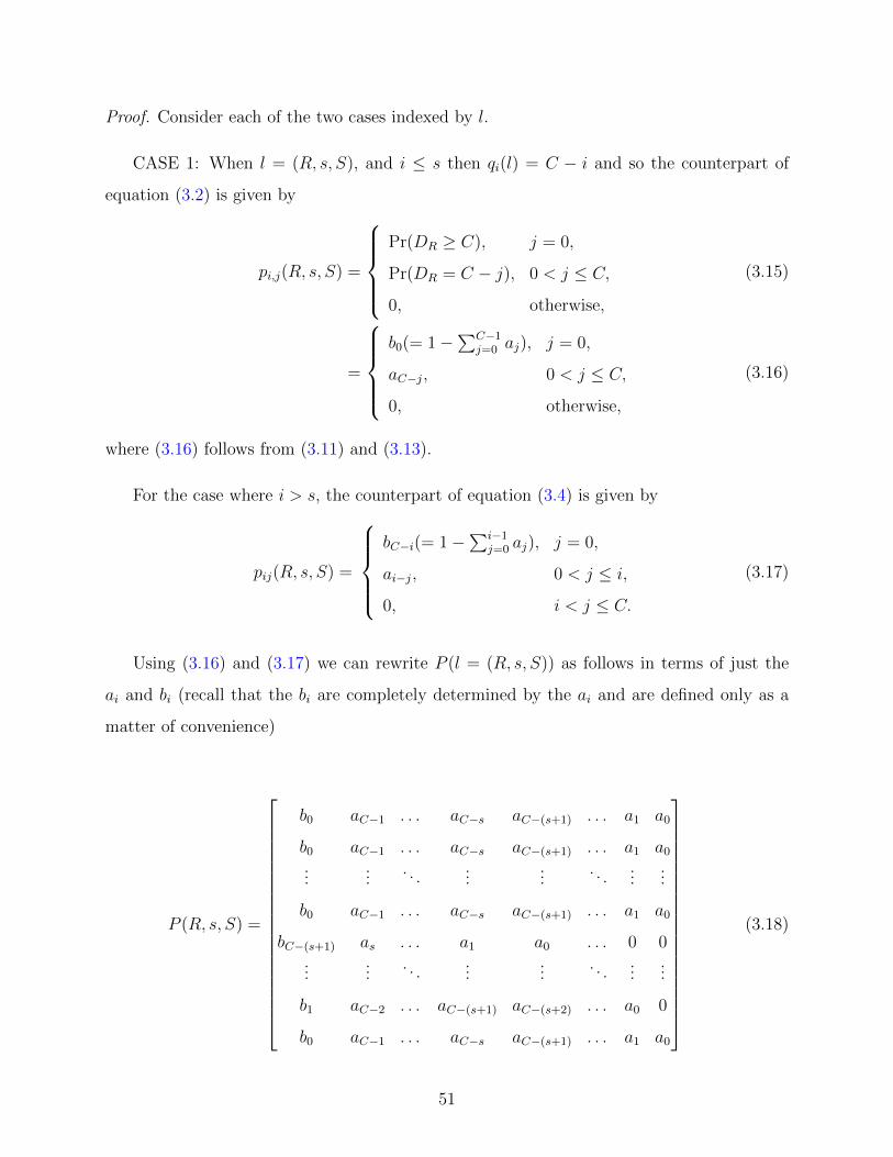
Proof. Consider each of the two cases indexed by l.
CASE 1: When l = (R, s, S), and i ≤ s then qi(l) = C − i and so the counterpart of
equation (3.2) is given by
pi,j(R, s, S) =
Pr(DR ≥ C), j = 0,
Pr(DR = C − j), 0 < j ≤ C,
0, otherwise,
(3.15)
=
b0(= 1−
∑C−1j=0 aj), j = 0,
aC−j, 0 < j ≤ C,
0, otherwise,
(3.16)
where (3.16) follows from (3.11) and (3.13).
For the case where i > s, the counterpart of equation (3.4) is given by
pij(R, s, S) =
bC−i(= 1−
∑i−1j=0 aj), j = 0,
ai−j, 0 < j ≤ i,
0, i < j ≤ C.
(3.17)
Using (3.16) and (3.17) we can rewrite P (l = (R, s, S)) as follows in terms of just the
ai and bi (recall that the bi are completely determined by the ai and are defined only as a
matter of convenience)
P (R, s, S) =
b0 aC−1 . . . aC−s aC−(s+1) . . . a1 a0
b0 aC−1 . . . aC−s aC−(s+1) . . . a1 a0
......
. . ....
.... . .
......
b0 aC−1 . . . aC−s aC−(s+1) . . . a1 a0
bC−(s+1) as . . . a1 a0 . . . 0 0...
.... . .
......
. . ....
...
b1 aC−2 . . . aC−(s+1) aC−(s+2) . . . a0 0
b0 aC−1 . . . aC−s aC−(s+1) . . . a1 a0
(3.18)
51

CASE 2: When l = (R, s,Q), and i ≤ s then qi(l) = C − s and so the counterpart of
equation (3.2) is given by
pi,j(R, s,Q) =
Pr(DR ≥ i+ C − s), j = 0,
Pr(DR = i+ C − s− j), 0 < j ≤ i+ C − s,
0, otherwise,
(3.19)
=
bs−i(= 1−
∑C−(s−i+1)j=0 aj), j = 0,
ai+C−s−j, 0 < j ≤ C − s+ i,
0, otherwise,
(3.20)
(3.20) follows from (3.11) and (3.13).
For the case where i > s, the counterpart of equation (3.4) is given by
pij(R, s,Q) =
bC−i(= 1−
∑i−1j=0 aj), j = 0,
ai−j, 0 < j ≤ i,
0, i < j ≤ C.
(3.21)
Similar to the first case, using (3.20) and (3.21) we can rewrite P (l = (R, s,Q)) in terms of
just the ai and bi:
P (R, s,Q) =
bs aC−(s+1) . . . aC−2s aC−2s−1 . . . 0 0
bs−1 aC−s . . . aC−2s+1 aC−2s . . . 0 0...
.... . .
......
. . ....
...
b0 aC−1 . . . aC−s aC−(s+1) . . . a1 a0
bC−(s+1) as . . . a1 a0 . . . 0 0...
.... . .
......
. . ....
...
b1 aC−2 . . . aC−(s+1) aC−(s+2) . . . a0 0
b0 aC−1 . . . aC−s aC−(s+1) . . . a1 a0
(3.22)
Note that because (3.17) and (3.21) are identical, the sub-matrix in rows s+ 1 and higher is
the same for either policy. This should be intuitively clear because if we are not placing an
order at the current review point then the state of the process at the next review point will
only depend on the total demand during the current review period and not on the policy in
use or the lead time.
52

Matrices for (R, s = 4, S = 12) and (R, s = 4, Q = 8) are added to the appendix B as an
example.
Corollary 1. The transition probability matrix P has the following characteristics:
1. The last row of the transition matrix for any policy with any lead time is always a
2. When s = 0, all rows of P except for the first row (corresponding to i = 0) are identical
across all policies.
3. When L = 0 and we are using an (R, s, S) policy, the transition probabilities for all states
less than or equal to the reorder point s are identical and given by a.
4. When s = C − 1 in the (R, s, S) policy, all rows of the transition matrix are identical
and given by a; therefore, we can conclude that its limiting probability distribution is also
given by a.
5. With the (R, s, S) policy, all elements of b only appear once for s = 0.
Proof. 1. The entry in column j of the last row is pCj. If i = C then regardless of the policy
in use we will not place an order at the current review point and so the probability of
being in state j at the next review point depends only on the total demand in the current
review period as given by aj and is independent of the policy or the lead time.
2. If s = 0, then for all i > 0, the identical equations (3.17) and (3.21) are used to calculate
transition probabilities, and this does not depend on L, s or the policy type.
3. All transition probabilities in P (R, s, S) when i ≤ s are derived from equation (3.16),
which is identical for every i.
4. Follows from clauses (1) and (3); note that this is the so-called PAR policy that is
commonly used in many hospital settings.
5. Follows from clause (3).
In order to exactly compute the limiting probability distribution, we need to show that
our DTMC is ergodic. In the following lemma, we prove that this is true for both policies
considered.
53
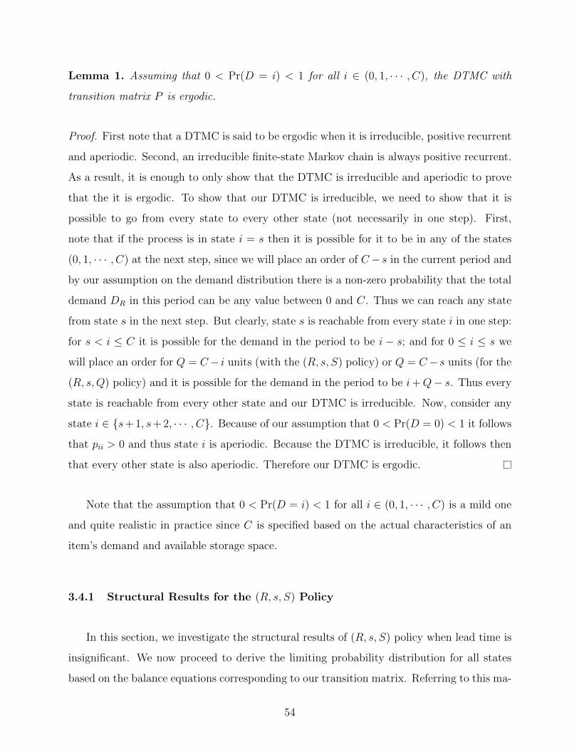
Lemma 1. Assuming that 0 < Pr(D = i) < 1 for all i ∈ (0, 1, · · · , C), the DTMC with
transition matrix P is ergodic.
Proof. First note that a DTMC is said to be ergodic when it is irreducible, positive recurrent
and aperiodic. Second, an irreducible finite-state Markov chain is always positive recurrent.
As a result, it is enough to only show that the DTMC is irreducible and aperiodic to prove
that the it is ergodic. To show that our DTMC is irreducible, we need to show that it is
possible to go from every state to every other state (not necessarily in one step). First,
note that if the process is in state i = s then it is possible for it to be in any of the states
(0, 1, · · · , C) at the next step, since we will place an order of C− s in the current period and
by our assumption on the demand distribution there is a non-zero probability that the total
demand DR in this period can be any value between 0 and C. Thus we can reach any state
from state s in the next step. But clearly, state s is reachable from every state i in one step:
for s < i ≤ C it is possible for the demand in the period to be i − s; and for 0 ≤ i ≤ s we
will place an order for Q = C− i units (with the (R, s, S) policy) or Q = C−s units (for the
(R, s,Q) policy) and it is possible for the demand in the period to be i+Q− s. Thus every
state is reachable from every other state and our DTMC is irreducible. Now, consider any
state i ∈ {s+ 1, s+ 2, · · · , C}. Because of our assumption that 0 < Pr(D = 0) < 1 it follows
that pii > 0 and thus state i is aperiodic. Because the DTMC is irreducible, it follows then
that every other state is also aperiodic. Therefore our DTMC is ergodic.
Note that the assumption that 0 < Pr(D = i) < 1 for all i ∈ (0, 1, · · · , C) is a mild one
and quite realistic in practice since C is specified based on the actual characteristics of an
item’s demand and available storage space.
3.4.1 Structural Results for the (R, s, S) Policy
In this section, we investigate the structural results of (R, s, S) policy when lead time is
insignificant. We now proceed to derive the limiting probability distribution for all states
based on the balance equations corresponding to our transition matrix. Referring to this ma-
54

trix (18), the corresponding equation for j = 0 and for each j ∈ {0, 1, · · · s} are respectively
given by
π0 = b0
(s∑i=0
πi
)+
C∑i=s+1
bC−iπi (3.23)
πj =∑i
πiPij,
=∑i≤s
Pijπi +∑i>s
Pijπi,
= aC−j
(s∑i=0
πi
)+
C∑i=s+1
ai−jπi (3.24)
Now consider the balance equations corresponding to a state j ∈ {s + 1, s + 2, · · ·C}. This
is given by
πj = Pjjπj +∑i 6=j
πiPij,
= Pjjπj +∑i≤s
Pijπi +∑
i>s,i 6=j
Pijπi,
= a0πj + aC−j
(∑i≤s
πi
)+
C∑i=j+1
ai−jπi (3.25)
Note that (3.25) follows from the fact that for i > s, the value of Pij is equal to 0 for i < j,
and equal to a0 for i = j. It now follows that
(1− a0)πj = aC−j
(∑i≤s
πi
)+
C∑i=j+1
ai−jπi, (3.26)
⇒ πj∑i≤s πi
=aC−j
1− a0
+C∑
i=j+1
ai−j1− a0
(πi
(∑
i≤s πi)
)(3.27)
As a matter of notational convenience, let us define the following:
Definition 3.
γj =πj∑i≤s πi
, j ∈ {s+ 1, · · · , C} (3.28)
ρi =ai
1− a0
, i ∈ {0, · · · , C} (3.29)
55
Thus, equations (3.27) for j ∈ {s+ 1, s+ 2, · · · , C} can be rewritten as
γj = ρC−j +C∑
i=j+1
ρi−jγi (3.30)
We now state and prove the main proposition in this section, which provides a closed-form
for the values of γs+1, γs+2, · · · , γC that uses just the vector a as given by (3.11) (as we
will show subsequently, these values can in turn be used to determine a closed-form for the
limiting probability vector π). The approach is based on decomposing the set of states into
two mutually exclusive subsets: (1) j ∈ {0, 1, · · · , s}, and (2) j ∈ {s+ 1, · · · , C}, i.e., values
smaller than or equal to the reorder point and values larger than the reorder point. We will
focus initially on the second subset.
To motivate the development of this proposition, consider the application of (3.30) for
values of j = C,C − 1, ....
γC = ρ0
=a0
1− a0
γC−1 = ρ1 + ρ1γC
= ρ1(1 + γC)
= ρ1(1
1− a0
)
=1
(1− a0)(1!
1!)ρ1
γC−2 = ρ2(1 + γC) + ρ1γC−1
=ρ2
1− a0
+ρ2
1
1− a0
=1
(1− a0)
((1!
1!)ρ2 + (
2!
2!)ρ2
1
)=
1
(1− a0)
((1!
1!)ρ0
1ρ12 + (
2!
2!)ρ2
1ρ02
)
=1
(1− a0)
∑n∈Z2
+|n1+2n2=2
(n1 + n2)!
n1!n2!ρn1
1 ρn22
56

γC−3 = ρ3(1 + γC) + ρ1γC−2 + ρ2γC−1
=ρ3
1− a0
+ ρ1(ρ2 + ρ2
1)
1− a0
+ ρ2ρ1
1− a0
=1
(1− a0)(ρ3 + 2ρ1ρ2 + ρ3
1)
=1
(1− a0)
((1!
1!)ρ3 + (
2!
1!1!)ρ1ρ2 + (
3!
3!)ρ3
1
)=
1
(1− a0)
((1!
1!)ρ0
1ρ02ρ
13 + (
2!
1!1!)ρ1
1ρ12ρ
03 + (
3!
3!)ρ3
1ρ02ρ
03
)
=1
(1− a0)
∑n∈Z3
+|n1+2n2+3n3=3
(n1 + n2 + n3)!
n1!n2!n3!ρn1
1 ρn22 ρ
n33
γC−4 = ρ4(1 + γC) + ρ1γC−3 + ρ2γC−2 + ρ3γC−1
=ρ4
1− a0
+ ρ1(ρ3 + 2ρ1ρ2 + ρ3
1)
1− a0
+ ρ2(ρ2 + ρ2
1)
1− a0
+ ρ3ρ1
1− a0
=1
(1− a0)(ρ4 + 2ρ1ρ3 + ρ2
2 + 3ρ21ρ2 + ρ4
1)
=1
(1− a0)
((1!
1!)ρ4 + (
2!
1!1!)ρ1ρ3 + (
2!
2!)ρ2
2 + (3!
2!1!)ρ2
1ρ2 + (4!
4!)ρ4
1
)=
1
(1− a0)
((1!
1!)ρ0
1ρ02ρ
03ρ
14 +
((
2!
1!1!)ρ1
1ρ02ρ
13ρ
04 + (
2!
2!)ρ0
1ρ22ρ
03ρ
04
)+ (
3!
2!1!)ρ2
1ρ12ρ
03ρ
04 + (
4!
4!)ρ4
1ρ02ρ
03ρ
04
)
=1
(1− a0)
∑n∈Z4
+|∑4
k=1 knk=4
(∑4
k=1 nk)!∏4k=1 nk!
4∏k=1
ρnkk
Observing the pattern above, we may now generalize this to the following proposition.
Proposition 3. The values of γC−d =πC−d∑i≤s πi
are given by
γC =a0
(1− a0); d ∈ {0} (3.31)
and
γC−d =1
(1− a0)
∑n∈Zd
+|∑d
k=1 knk=d
(∑d
k=1 nk)!∏dk=1 nk!
d∏k=1
ρnkk
; d ∈ {1, 2, · · · , C − (s+ 1)} (3.32)
57

Proof. Our focus is on states j ∈ {s+ 1, · · · , C}, i.e., we consider values of d = 0, 1, · · · , C−
(s + 1) to find γC−d. First, note that (3.31) corresponding to d = 0 follows trivially from
(3.30) and (3.29). For d = 1, 2, · · · , C − (s + 1) we will prove (3.32) using strong induction
on d. Consider the base case with d = 1. Using (3.30) we have
γC−1 = ρ1 + ρ1γC
= ρ1(1 + γC)
= ρ1(1
1− a0
)
=1
(1− a0)(1!
1!)ρ1
This shows that equation (3.32) holds for d = 1. Now consider some arbitrary m ∈
{2, 3, · · · , C − (s + 2)}, and for the strong induction step, suppose that ((3.32)) holds for
d = 1, 2, · · · ,m. It suffices to prove that (3.32) also holds for d = m + 1. Note that based
on its definition in (3.28), γj is not defined for values of j < s+ 1 or equivalently γC−d is not
defined for values of d > C − (s+ 1). Corresponding to m we have
γC−m =1
(1− a0)
∑n∈Zm
+ |∑m
k=1 knk=m
(∑m
k=1 nk)!∏mk=1 nk!
m∏k=1
ρnkk
(3.33)
Now consider equation (3.30) for j = C − (m+ 1)
γC−(m+1) = ρm+1 +C∑
i=C−m
ρ(i−C+m+1)γi (3.34)
It is easily seen that this may be re-indexed and rewritten as
γC−(m+1) = ρm+1 +m∑i=0
ρ(m+1−i) γC−i (3.35)
Based on the strong induction assumption let us substitute the values for γC−d; d ∈ {1, 2, · · · , C−
m} obtained from equation (3.32) and for γC from ((3.31)), into equation (3.35). This yields
γC−(m+1) = ρm+1 + ρm+1a0
1− a0
+1
(1− a0)
m∑i=1
ρm+1−i
∑n∈Zi
+|∑i
k=1 knk=i
(∑i
k=1 nk)!∏ik=1 nk!
i∏k=1
ρnkk
=
1
1− a0
ρm+1 +1
(1− a0)
m∑i=1
ρm+1−i
∑n∈Zi
+|∑i
k=1 knk=i
(∑i
k=1 nk)!∏ik=1 nk!
i∏k=1
ρnkk
(3.36)
58

Now consider the vectors n ∈ Zi+ |∑i
k=1 knk = i that determine the domain for the in-
ner summation in (3.36) above. Noting that i ≤ m, we can instead write this domain as
n ∈ Zm+ |∑m
k=1 knk = i, because any n ∈ Zm+ that satisfies n1 + 2n2 + ...ini + ...mnm = i
must have ni+1 = ni+2 = · · · = nm = 0. The quantity within the summation is of course
unaffected by this because ρ0k = 1 and 0! = 1. This allows us to rewrite (3.36) as
γC−(m+1) =1
1− a0
ρm+1 +1
(1− a0)
m∑i=1
ρm+1−i
∑n∈Zm
+ |∑m
k=1 knk=i
(∑m
k=1 nk)!∏mk=1 nk!
m∏k=1
ρnkk
(3.37)
Now consider the expression within the outer summation:
ρm+1−i
∑n∈Zm
+ |∑m
k=1 knk=i
(∑m
k=1 nk)!∏mk=1 nk!
m∏k=1
ρnkk
=∑
n∈Zm+ |
∑mk=1 knk=i
(∑m
k=1 nk)!∏mk=1 nk!
ρm+1−i
m∏k=1
ρnkk
Since 1 ≤ i ≤ m in this summation, we also have 1 ≤ (m+1−i) ≤ m. In other words ρm+1−i
also appears in the product∏m
k=1 ρnkk , and if ρ(m+1−i) were to be pulled into the product it
would have an exponent of 1 + nm+1−i. For ease of notation let us define
nm+1−i = 1 + nm+1−i;nk = nk, k 6= (m+ 1− i) (3.38)
This allows us to rewrite
ρm+1−i
m∏k=1
ρnkk =
m∏k=1
ρnkk (3.39)
In order to also restate the(∑m
k=1 nk)!∏mk=1 nk!
portion (so that the summation can now be all in terms
of n) we will use some basic algebra. If
m∑k=1
knk = i
59

then
(m+ 1− i) +m∑k=1
knk = i+ (m+ 1− i)
(m+ 1− i) + (m+ 1− i)nm+1−i +m∑
k=1,k 6=m+1−i
knk = m+ 1
(m+ 1− i)(1 + nm+1−i) +m∑
k=1,k 6=m+1−i
knk = m+ 1
m∑k=1
knk = m+ 1 (3.40)
Also, using some simple algebra
(∑m
k=1 nk)!∏mk=1 nk!
=(n1 + · · ·+ nm+1−i + · · ·+ nm)!
n1! · · ·nm+1−i! · · ·nm!(3.41)
=(n1 + · · ·+
(nm+1−i + 1
)+ · · ·+ nm)!
1 +∑m
k=1 nk
nm+1−i + 1
n1! · · ·(nm+1−i + 1
)! · · ·nm!
=
(n(m+1−i)∑m
k=1 nk
)(∑m
k=1 nk)!∏mk=1 nk!
(3.42)
Using (3.39), (3.40) and (3.42) in equation (3.37), we have
γC−(m+1) =1
1− a0
ρm+1 +1
(1− a0)
m∑i=1
∑n∈Zm
+ |∑m
k=1 knk=m+1
(n(m+1−i)∑m
k=1 nk
)(∑m
k=1 nk)!∏mk=1 nk!
m∏k=1
ρnkk
Changing the order of the summation in the RHS this yields
γC−(m+1) =1
1− a0
ρm+1 +1
(1− a0)
∑n∈Zm
+ |∑m
k=1 knk=m+1
(m∑i=1
n(m+1−i)∑mk=1 nk
)(∑m
k=1 nk)!∏mk=1 nk!
m∏k=1
ρnkk
=
1
1− a0
ρm+1 +1
(1− a0)
∑n∈Zm
+ |∑m
k=1 knk=m+1
1 · (∑m
k=1 nk)!∏mk=1 nk!
m∏k=1
ρnkk
=
1
1− a0
1!
1!ρm+1 +
∑n∈Zm
+ |∑m
k=1 knk=m+1
(∑m
k=1 nk)!∏mk=1 nk!
m∏k=1
ρnkk
=
1
1− a0
∑n∈Zm
+ |∑m
k=1 knk=m+1
(∑m+1
k=1 nk)!∏m+1k=1 nk!
m+1∏k=1
ρnkk
(3.43)
This completes the proof.
60

Note that the coefficient for∏
k ρk is the so-called multinomial coefficient and using the
notation that is common for the latter, could be denoted as follows:
(∑m+1
k=1 nk)!∏m+1k=1 nk!
=
( ∑m+1k=1 nk
n1, n2, · · · , nm+1
)(3.44)
Let us use Proposition 3 to compute γj for all j ∈ {s+1, s+2, · · · , C}, and in particular, the
sum of these values. Then we can directly compute the exact value of the limiting probability
πj for j ∈ {0, 1, · · · , C} using the very simple formulas in the following two propositions;
the first computes values of πj for j ∈ {s + 1, s + 2, · · · , C} and the second uses these to
compute values of πj for j ∈ {0, 1, · · · , s}.
Proposition 4. The values of the limiting probability πj for j ∈ {s + 1, s + 2, · · · , C} are
given by
πj =γj
1 +∑C
i=s+1 γi(3.45)
Proof. First note that we can rewrite∑C
j=0 πj = 1 as
s∑j=0
πj +C∑
j=s+1
πj = 1
∑sj=0 πj∑sj=0 πj
+
∑Cj=s+1 πj∑sj=0 πj
=1∑sj=0 πj
1 +C∑
j=s+1
πj∑si=0 πi
=1∑sj=0 πj
1 +C∑
j=s+1
γj =1∑sj=0 πj
s∑i=0
πi =1
1 +∑C
j=s+1 γj(3.46)
But from (3.28) in Definition 3 we had πj = γj∑s
i=0 πi. Then it follows that
πj =γj
1 +∑C
i=s+1 γi(3.47)
This completes the proof.
61

Proposition 5. The values of the limiting probability πj for j = 0 and j ∈ {1, · · · , s} are
given respectively, by
π0 = b0
(1
1 +∑C
i=s+1 γi
)+
C∑i=s+1
bC−iπi (3.48)
and
πj = aC−j
(1
1 +∑C
i=s+1 γi
)+
C∑i=s+1
ai−jπi (3.49)
Proof. Follows directly from (3.46), (3.23) and (3.24).
Before proceeding to develop an efficient algorithm for computing the exact limiting prob-
ability distribution for various values of s, let us use πj(s) to denote the limiting probability
corresponding to state j, given that we are using an (R, s, S) policy with s as its reorder
point. Let us also use γj(s) in a similar fashion to denote the value of γj corresponding to
a given s. We introduce two new lemmas now. The first establishes the fact that we can
re-use values of γj computed for some reorder point when we need these values for smaller
reorder points.
Lemma 2. Suppose s1 and s2, where s1 > s2, correspond to two different reorder points for
the same (R, s, S = C) system. The the following equation holds for all j ∈ {s1 + 1, · · · , C},
γj(s1) = γj(s2) (3.50)
Proof. The results follow directly from Proposition 3; (3.31) and (3.32) are identically defined
for both s1 and s2 when d ∈ {0, 1, · · · , C − (s1 + 1)}.
The second lemma establishes a relationship between the limiting distributions for adja-
cent values of the reorder point that can be exploited in a recursive algorithm.
Lemma 3. In an (R, s, S) system with zero lead time, the following equation holds:∑s−1i=0 πi(s− 1)∑si=0 πi(s)
= 1− πs(s− 1)
62

Proof. Using Lemma 2 with s1 = s and s2 = s− 1 and (3.28) we have for all j ∈ {s+ 1, s+
2, · · · , C}
πj(s− 1)∑s−1i=0 πi(s− 1)
=πj(s)∑si=0 πi(s)
, (3.51)
Therefore
C∑j=s+1
πj(s− 1)∑s−1i=0 πi(s− 1)
=C∑
j=s+1
πj(s)∑si=0 πi(s)
,
∑Ci=s+1 πi(s− 1)∑s−11=0 πi(s− 1)
=
∑Ci=s+1 πi(s)∑si=0 πi(s)
(3.52)
Now, consider the limiting probabilities for the (R, s− 1, S = C) system.
C∑i=0
πi(s− 1) = 1,
s−1∑i=0
πi(s− 1) +C∑
i=s+1
πi(s− 1) = 1− πs(s− 1),
s−1∑i=0
πi(s− 1)
(1 +
∑Ci=s+1 πi(s− 1)∑s−1i=0 πi(s− 1)
)= 1− πs(s− 1), (3.53)
Substituting from (3.52) in equation (3.53) we obtain
s−1∑i=0
πi(s− 1)
(1 +
∑Ci=s+1 πi(s)∑si=0 πi(s)
)= 1− πs(s− 1), (3.54)
s−1∑i=0
πi(s− 1)
(∑si=0 πi(s) +
∑Ci=s+1 πi(s)∑s
i=0 πi(s)
)= 1− πs(s− 1),∑s−1
i=0 πi(s− 1)∑si=0 πi(s)
= 1− πs(s− 1),
where the last equation follows from the fact that the sum in the numerator of the fraction
in the penultimate equation is∑C
i=0 πi(s) = 1.
We now derive the following theorem using Lemmas 2 and 3; this theorem forms the basis
for an efficient recursive algorithm that starts with the limiting distribution for s = C − 1
and proceeds to compute the limiting distributions for s = C − 2, C − 3, · · · , 0.
63

Theorem 4. Given an (R, s, S) system with L = 0 and the limiting probability distribution
π(s) corresponding to some s, the limiting probability distribution π(s− 1) corresponding to
s− 1 may be computed as follows:
For j ∈ {s, · · · , C}
πj(s− 1) =
πs(s)
1− a0 + πs(s)if j = s,
(1− a0)πj(s)
1− a0 + πs(s)if s < j ≤ C,
(3.55)
For j ∈ {1, · · · , s− 1}
πj(s− 1) = aC−j +C∑k=s
(ak−j − aC−j)πk(s− 1) (3.56)
Proof. We start with j ∈ {s, · · · , C}. Consider the balance equation for πs(s − 1) (when
j = s) in the form given by equation (3.27) and then apply equation (3.51) to obtain
πs(s− 1)∑i≤s−1 πi(s− 1)
=aC−s
1− a0
+C∑
i=s+1
ai−s1− a0
(πi(s− 1)
(∑
i≤s−1 πi(s− 1))
)
(1− a0)πs(s− 1)∑s−1i=0 πi(s− 1)
= aC−s +C∑
i=s+1
ai−sπi(s− 1)∑s−1i=0 πi(s− 1)
(1− a0)πs(s− 1)∑s−1i=0 πi(s− 1)
= aC−s +C∑
i=s+1
ai−sπi(s)∑si=0 πi(s)
, (3.57)
Now consider (3.24) corresponding to j = s for the (R, s, S = C) system. If we divide both
sides of (3.24) by∑s
i=0 πi(s) the RHS is identical to the RHS of (3.57) above. Thus we may
rewrite (3.57) as
(1− a0)πs(s− 1)∑s−1i=0 πi(s− 1)
=πs(s)∑si=0 πi(s)
,
(1− a0)πs(s− 1) = πs(s)
∑s−1i=0 πi(s− 1)∑si=0 πi(s)
(3.58)
64

Applying Lemma 3 to equation (3.58) then yields
(1− a0)πs(s− 1) = πs(s)(
1− πs(s− 1)),
πs(s− 1) =πs(s)
1− a0 + πs(s)(3.59)
This completes the proof for j = s. Now consider some j > s. We start by using Lemma 2
and (3.28) to obtain
πj(s− 1)∑s−1i=0 πi(s− 1)
=πj(s)∑si=0 πi(s)
,
πj(s− 1) = πj(s)(∑s−1
i=0 πi(s− 1)∑si=0 πi(s)
)
Now, first applying Lemma 3 to the expression within parentheses in the RHS, and then
applying (3.59) for the value of πs(s− 1) we obtain
πj(s− 1) = πi(s)(
1− πs(s− 1))
πj(s− 1) =(1− a0)πj(s)
1− a0 + πs(s)(3.60)
This completes the proof for j ∈ {s+ 1, s+ 2, · · · , C}. To compute the limiting probabilities
for j ∈ {1, 2, · · · , s− 1} consider the balance equation for πj as given by (3.24).
πj(s− 1) = aC−j
(s−1∑i=0
πi(s− 1)
)+
C∑i=s
ai−jπi(s− 1)
= aC−j
(1−
C∑i=s
πi(s− 1)
)+
C∑i=s
ai−jπi(s− 1)
= aC−j +C∑i=s
(ai−j − aC−j)πi(s− 1)
65

The limiting probabilities corresponding to any given s may be computed by using Propo-
sitions 4 and 5. However, these require the computation of the closed-form for γj as given by
Proposition 3. While this is easy to do when values of s are close to C it becomes increas-
ingly difficult for values of s that are significantly smaller than C. Note that enumerating all
vectors n ∈ Zk+ that satisfy n1 +2n2 + · · ·+knk = k is a combinatorial problem, and as C−s
increases, the value of k also increases and makes this task more difficult. We therefore take
an alternative approach and propose an algorithm that starts by computing π(C−1), which
is trivial to do, and then uses Theorem 4 to recursively compute π(C − 2),π(C − 3), · · · .
This algorithm is very efficient and only requires the values of the the vectors a and b as
given by (3.11) and (3.13) respectively, which is a simple one-time calculation. Moreover,
the algorithm provides us with the limiting probability distribution corresponding to every
value of s between 0 and C − 1.
Algorithm 1. The following steps may be used to find the limiting probability distributions
π(s) for s ∈ {C − 1, C − 2, · · · , 0}:
1. Set s = C − 1, and compute πj(C − 1) = aC−j, ∀j ∈ {1, · · · , C} and π0(C − 1) =
1−∑C−1
i=0 ai = b0; this yields π(C − 1).
2. Find πj(s− 1), for all j ∈ {s, · · · , S} using the previously computed values of π(s) and
equation (3.55) from Theorem 4.
3. Using the results of the previous step, find πj(s− 1) for 1 ≤ j < s − 1 using equation
(3.56) from Theorem 4 and then π0(s − 1) = 1 −∑C
j=1 πj; the end of this step yields
π(s− 1).
4. If s = 0, exit the algorithm; otherwise, if s = C − 1 set s = s− 2, else set s = s− 1 and
return to step 2.
In Step 1 we use Propositions 4 and 5 with the value of γC−1 computed via Proposition 3.
In steps 2 and 3 we use Theorem 4 to recursively compute the values of π(C−2), π(C−3) · · ·
using π(C − 1), π(C − 2) · · · , respectively. Also, note that the first time we execute Step 4,
s = C − 1 and we already have the value of π(s − 1 = C − 2) so we decrement s by 2 to
next find π(C − 3); at subsequent iterations we decrement it by 1.
66
3.4.2 Structural Results for the (R, s,Q) Policy
We now turn to the (R, s,Q) system. With a maximum limit on the amount of inventory
(C) we can have at any one time the order quantity we will use is determined by the reorder
point s via Q = C − s. In this system, having a large value for s along with a small order
quantity can result in poor service. For example, consider an extreme case where s = C − 1
so that Q = 1. In this instance orders will be placed in almost every cycle. However,
since the order quantity is equal to 1, there will be many cycles where we start with much
fewer than C items and eventually there will be many cycles where we stock out. Given
that service levels are specified as fairly high values, we therefore make the assumption that
the reorder point is smaller than C2
, so that the order quantity Q is larger thanC
2. Other
researchers have also set similar limits for s with an (R, s,Q) policy (e.g., Bijvank and Vis
(2012b) and Bijvank and Vis (2012a)). In order for this policy to be stable, one approach is
to set the difference between the reorder point and C to be greater than reorder point. So
this requirement that C − s > s leads to s < C2
.
We now proceed to derive the limiting probability distribution for all states based on the
balance equations corresponding to our transition matrix for (R, s,Q) as given by (3.22),
starting with s < j ≤ C. Referring to the structure of this matrix and given our assumption
that s < C2
, the corresponding equations will be described separately for values of j such
that s < j < C − s and j such that C − s ≤ j ≤ C.
We consider the latter case first, i.e., C − s ≤ j ≤ C. Note that for such j, as a result of
our assumption that s < C2
it follows that j > s. The corresponding steady-state equation
is given by
πj =∑i
πiPij,
=s∑i=0
Pijπi +C∑
i=s+1
Pijπi,
Note that in the first summation, where i ≤ s (3.20) applies and Pij = 0 if j > i + C − s,
i.e., when i < s− (C − j). So this summation ranges from s− (C − j) to s. Similarly, in the
67

second summation where (3.21) applies, Pij = 0 when i < j, so that this summation ranges
from j to C. Therefore we may rewrite the above equation as
πj =s∑
i=s−(C−j)
Pijπi +C∑i=j
Pijπi, (3.61)
=s∑
i=s−(C−j)
a(C−j)−(s−i) πi +C∑i=j
ai−jπi,
We now make a change in the index for the first summation from i to i− (C − s); therefore
for the lower and upper bounds of the summation we have:
s− (C − j) ≤ i ≤ s,
s− (C − j) + (C − s) ≤ i+ (C − s) ≤ s+ (C − s),
j ≤ i+ (C − s) ≤ C
It follows then that
πj =C∑i=j
ai−j πs−(C−i) +C∑i=j
ai−j πi, (3.62)
=C∑i=j
ai−j(πs−(C−i) + πi), (3.63)
= a0(πs−(C−j) + πj) +C∑
i=j+1
ai−j(πs−(C−i) + πi)
Rearranging this we obtain
(1− a0)πj = a0(πs−(C−j)) +C∑
i=j+1
ai−j(πs−(C−i) + πi),
πj =a0
1− a0
(πs−(C−j)) +C∑
i=j+1
ai−j1− a0
(πs−(C−i) + πi), (3.64)
= ρ0(πs−(C−j)) +C∑
i=j+1
ρi−j(πs−(C−i) + πi), (3.65)
68

Now consider the equation for j such that s+ 1 ≤ j < C − s.
πj =∑i
πiPij,
=s∑i=0
Pijπi +C∑
i=s+1
Pijπi,
Once again, note that in the second summation where (3.21) applies, Pij = 0 when i < j, so
that it only ranges from j to C; we further break this up into two parts: from j to C−(s+1)
and from (C − s) to C, and apply an index change as with the previous case. Thus
πj =s∑i=0
Pijπi +
C−(s+1)∑i=j
Pijπi +C∑
i=C−s
Pijπi, (3.66)
=s∑i=0
a(C−j)−(s−i) πi +
C−(s+1)∑i=j
ai−jπi +C∑
i=C−s
ai−jπi,
=C∑
i=C−s
a(i−j) πs−(C−i) +
C−(s+1)∑i=j
ai−jπi +C∑
i=C−s
ai−jπi,
=
C−(s+1)∑i=j
ai−jπi +C∑
i=C−s
ai−j(πs−(C−i) + πi), (3.67)
= a0πj +
C−(s+1)∑i=j+1
ai−jπi +C∑
i=C−s
ai−j(πs−(C−i) + πi),
Rearranging this we obtain
(1− a0)πj =
C−(s+1)∑i=j+1
ai−jπi +C∑
i=C−s
ai−j(πs−(C−i) + πi),
πj =
C−(s+1)∑i=j+1
ai−j1− a0
πi +C∑
i=C−s
ai−j1− a0
(πs−(C−i) + πi), (3.68)
=
C−(s+1)∑i=j+1
ρi−j πi +C∑
i=C−s
ρi−j (πs−(C−i) + πi), (3.69)
Before introducing the next proposition we revisit γj, j ∈ {s + 1, s + 2, · · · , C} as defined
by (3.28) in Definition 3 for which we derived the closed-forms given by (3.31) and (3.32)
in Proposition 3 when discussing the (R, s, S) system. For the rest of the discussion in this
section we will use these same values of γj. Note that the values computed using (3.31) and
69
(3.32) also satisfy (3.28) for the (R, s, S) system. However, these closed form expressions
themselves are independent of s, S and Q and are functions only of the aj values (recall
that the ρj in the closed form are functions of only the aj and are given by (3.29)). While
these values were derived for the (R, s, S) system we will also use them for deriving limiting
probabilities in the (R, s,Q) system. In effect, for the remainder of this section we may view
these values derived for the (R, s, S) system (and that follow all the relationships in the prior
section) as constants.
We now state and prove the following proposition.
Proposition 6. Assuming that s < C2
, we can compute the values of πC , πC−1, · · · , πs+1 via
πC−d =
min{s,d}∑i=0
γC−(d−i) πs−i; d ∈ {0, 1, · · · , C − (s+ 1)} (3.70)
Proof. Let us think of d as the distance of j from C, i.e., d = C − j. We divide the proof
into two parts: (i for all j such that C − s ≤ j ≤ C (i.e., 0 ≤ d ≤ s) and (ii), for all j such
that s+ 1 ≤ j ≤ C − (s+ 1) (i.e., s+ 1 ≤ d ≤ C − (s+ 1).
Part 1 : Here we consider states j ∈ {C − s, · · · , C}, i.e., values of d = 0, 1, · · · , s. We
will find each πC−d as a function of πs, πs−1, · · · , πs−d. The proof will use strong induction
on d. Consider the base case with d = 0. Using (3.65), 3.29 and 3.31 it then follows that
πC = ρ0πs
=a0
1− a0
πs (3.71)
= γC πs, (3.72)
Thus equation (3.70) holds for d = 0. Now consider some arbitrary m ∈ {1, 2, · · · , s − 1},
and for the strong induction step, suppose that (3.70) also holds for d = 1, 2, · · · ,m. It
suffices for the first part to prove that (3.70) also holds for d = m + 1. Corresponding to
i ∈ {1, 2, · · · ,m} we have
πC−i =i∑
k=0
γC−(i−k) πs−k (3.73)
70
Now consider equation (3.65) for j = C − (m+ 1)
πC−(m+1) = ρ0(πs−(m+1)) +C∑
i=C−m
ρi−(C−(m+1)(πs−(C−i) + πi) (3.74)
Noting that ρ0 = γC and re-indexing the summation we can rewrite this as
πC−(m+1) = γC(πs−(m+1)) +m∑i=0
ρm+1−i(πs−i + πC−i) (3.75)
Based on the strong induction assumption let us substitute the values for πC−i; i ∈ {1, · · · ,m}
obtained from equation (3.73) and for πC from ((3.72)), into equation (3.75). This yields
πC−(m+1) = γC(πs−(m+1)) +m∑i=0
ρm+1−i(πs−i +i∑
k=0
γC−(i−k) πs−k), (3.76)
= γC(πs−(m+1)) +m∑i=0
ρm+1−i πs−i +m∑i=0
i∑k=0
(ρm+1−i γC−(i−k)) πs−k, (3.77)
= γC(πs−(m+1)) +m∑i=0
ρm+1−i πs−i +m∑i=0
(m−i∑k=0
ρm+1−(k+i) γC−k
)πs−i, (3.78)
= γC(πs−(m+1)) +m∑i=0
(ρm+1−i +
m−i∑k=0
ρm+1−(k+i) γC−k
)πs−i, (3.79)
where equation (3.78) is re-indexed and rewritten from equation (3.77) in a way that the π’s
do not depend on k and only depend on i. We may rewrite equation (3.30) as the following,
γC−d = ρd +d−1∑k=0
ρ(d−k) γC−k. (3.80)
If we write equation (3.80) for d = (m+ 1− i), so we will have:
γC−(m+1−i) = ρm+1−i +m−i∑i=0
ρm+1−(k+i) γC−k. (3.81)
Now by using equations (3.78) and (3.81), we have
πC−(m+1) = γC(πs−(m+1)) +m∑i=0
γC−(m+1−i)πs−i, (3.82)
πC−(m+1) =m+1∑i=0
γC−(m+1−i)πs−i, (3.83)
71

and (3.83) completes the Part 1 of the proof.
Part 2 : We next look at states j ∈ {s + 1, · · · , C − (s + 1)}, i.e., we consider values of
d = s+ 1, · · · , C − (s+ 1). We will find each πC−d as a function of π0, π1, · · · , πs. Note that
min{s, d} = s in equation (3.70). Again, the proof will use strong induction on d. Consider
the base case with d = s+ 1. Using (3.69), we have
πC−(s+1) =C∑
i=C−s
γi−(C−(s+1)) (πs−(C−i) + πi), (3.84)
=s∑i=0
γs+1−i(πs−i + πC−i), (3.85)
=s∑i=0
γs+1−i(πs−i +i∑
k=0
γC−(i−k) πs−k), (3.86)
where, equation (3.85) is derived by re-indexing equation (3.84) and equation (3.86) follows
from the results of the first part of the proof. Now, by using the same approach that we used
to derive the summation in equation (3.82) from the summation in (3.76), we can reduce
equation (3.86) to the following:
πC−(s+1) =s∑i=0
γC−(s+1−i)πs−i. (3.87)
Thus (3.70) holds for the base case of d = s + 1. Now consider some arbitrary m ∈ {s +
2, · · · , C − (s + 2)}, and for the strong induction step, suppose that (3.70) also holds for
d ∈ {s+ 2, · · · ,m− 1,m}, i.e., corresponding to i ∈ {s+ 2, · · · ,m} we have
πC−i =s∑
k=0
γC−(i−k) πs−k. (3.88)
It suffices to prove that equation (3.70) also holds for d = m + 1. We first re-index and
rewrite equation (3.69) as follows:
πC−d =d−1∑k=s+1
ρd−k πC−k +s∑
k=0
ρd−k (πs−k + πC−k) (3.89)
Now consider equation(3.89) for d = (m+ 1):
πC−(m+1) =m∑
k=s+1
ρm+1−k πC−k +s∑
k=0
ρm+1−k (πs−k + πC−k) (3.90)
72
Now by using the strong induction assumption, we substitute the values for πC−k; i ∈
{s + 2, · · · ,m} obtained from equation (3.88) and for πC−(s+1) from (3.87), into the first
summation in the above equation. Similarly, in the the second summation, we substitute
the values of πC−k, k = 0, 1, · · · , s obtained in the first part of the proof. This yields the
following:
πC−(m+1) =m∑
k=s+1
ρm+1−k
s∑i=0
γC−(k−i) πs−i +s∑
k=0
ρm+1−k (πs−k +k∑i=0
γC−(k−i) πs−i)
=s∑
k=0
ρm+1−k πs−k +s∑
k=0
k∑i=0
ρm+1−kγC−(k−i) πs−i +m∑
k=s+1
s∑i=0
ρm+1−k γC−(k−i) πs−i
=s∑
k=0
ρm+1−k πs−k +s∑
k=0
( s−k∑i=0
ρm+1−(i+k)γC−i
)πs−k +
s∑k=0
( m∑i=s+1
ρm+1−k γC−(i−k)
)πs−k
=s∑
k=0
(ρm+1−k +
s−k∑i=0
ρm+1−(i+k)γC−i +m∑
i=s+1
ρm+1−k γC−(i−k)
)πs−k
=s∑
k=0
(ρm+1−k +
s−k∑i=0
ρm+1−(i+k)γC−i +m−k∑
i=s−k+1
ρm+1−(i+k) γC−i
)πs−k
=s∑
k=0
(ρm+1−k +
m−k∑i=0
ρm+1−(i+k)γC−i
)πs−k (3.91)
Now using equation (3.80) with d = m + 1− k for the expression within parentheses above
we obtain
=s∑
k=0
γC−(m+1−k) πs−k (3.92)
This completes the proof.
Next, let us first re-index equation (3.24) as follows:
πC−d = ad
(s∑i=0
πi
)+
C−(s+1)∑i=0
ad−iπC−i (3.93)
As a matter of notational convenience, let us extend the definition for γ in Definition 3 to
all j ∈ {0, · · · , s}. We may thus rewrite (3.93) as
γC−d = ad +
C−(s+1)∑i=0
ad−i γC−i (3.94)
73
Also, let us define the following:
Definition 4.
ζj =πjπ0
, j ∈ {0, · · · , C} (3.95)
Thus ζ0 = 1 and let us correspondingly redefine equation (3.70) using this new definition
as follows:
ζC−d =
min{s,d}∑i=0
ζC−(d−i) πs−i; d ∈ {0, 1, · · · , C − (s+ 1)} (3.96)
Recall that from our assumption, s < C2
. Therefore, the number of equations is no more
than half the total number of states when deriving the limiting probability distribution for
values of j between 0 and s. In the following, we will provide the final theorem for this
section which specifies the balance equations to be solved.
Proposition 7. Assuming that s < C2
, we can compute the values of ζ1, ζ2, · · · , ζs by solving
the following set of s equations:
ζC−d = γC−(d−s) +s−1∑i=0
γC−(d−i)ζs−i; d ∈ {C − s, · · · , C − 1}. (3.97)
Proof. We will use Proposition 6 to prove this theorem. We start by writing balance equations
for all C−d where d ∈ {C−s, · · · , C−1} based on the corresponding matrix that we defined
at the beginning of the section.
πC−d =s∑
k=0
ad−k πs−k +
C−(s+1)∑k=s+1
ad−kπC−k +s∑
k=0
ad−kπC−k,
=s∑
k=0
ad−k πs−k +
C−(s+1)∑k=s+1
ad−k
( s∑i=0
γC−(k−i) πs−i
)+
s∑k=0
ad−k
( k∑i=0
γC−(k−i) πs−i
),
=s∑
k=0
ad−k πs−k +s∑
k=0
( C−(s+1)∑i=s+1
ad−i γC−(i−k)
)πs−k +
s∑k=0
( k∑i=0
ad−kγC−(k−i) πs−i
),
=s∑
k=0
ad−k πs−k +s∑
k=0
( C−(s+1)∑i=s+1
ad−i γC−(i−k)
)πs−k +
s∑k=0
( s−k∑i=0
ad−(i+k)γC−i
)πs−k,
(3.98)
74

Re-indexing the inner summations, we get
πC−d =s∑
k=0
ad−k πs−k +s∑
k=0
( C−(s+k)−1∑i=s−k+1
ad−(i+k) γC−i
)πs−k +
s∑k=0
( s−k∑i=0
ad−(i+k)γC−i
)πs−k,(3.99)
=s∑
k=0
ad−k πs−k +s∑
k=0
( C−(s+k)−1∑i=0
ad−(i+k)γC−i
)πs−k,
=s∑
k=0
(ad−k +
C−(s+k)−1∑i=0
ad−(i+k)γC−i
)πs−k,
=s∑
k=0
γC−(d−k)πs−k (3.100)
where the final equation is obtained by applying equation (3.94). If we now divide equation
(3.100) by π0 we obtain ζC−d as the following:
ζC−d =s∑
k=0
γC−(d−k)ζs−k,
= γC−(d−s) +s−1∑k=0
γC−(d−k)ζs−k. (3.101)
Theorem 5. The values of the limiting probability πj for j = 0 and j ∈ {1, · · · , C} are
given respectively, by
π0 =1
1 +∑C
i=1 ζi(3.102)
and
πj = π0ζj (3.103)
75

Proof. First note that we can rewrite∑C
j=0 πj = 1 as
π0 +C∑j=1
πj = 1
π0
π0
+
∑Cj=1 πj
π0
=1
π0
1 +C∑j=1
πjπ0
=1
π0
1 +C∑j=1
ζj =1
π0
π0 =1
1 +∑C
j=1 ζj(3.104)
The values of ζC−d for all d ∈ {C− s, · · · , C− 1} where d = C− j such as j ∈ {1, · · · , s} are
derived by Proposition 7. By substituting these values into equation (3.96), we can derive
values of ζC−d for all d ∈ {0, · · · , C − (s+ 1)} where d = C − j such as j ∈ {s+ 1, · · · , C}.
By substituting these values into equation (3.104), π0 is derived. From definition 4 we had
πj = ζjπ0 and this completes the proof.
3.5 NUMERICAL ANALYSIS
In this section, we have five different subsections. First, we illustrate the intuitive fact
that when lead time is high, service level will be low and that when lead times are small
the performance of a policy is very close to the performance of a policy with L = 0. This
holds with both (R, s, S) and (R, s,Q) policies. Next, we illustrate the fact that determining
whether (R, s, S) or (R, s,Q) is better in a particular setting is not a trivial task and depends
on the relative magnitudes of the costs associated with replenishment and counting. Third,
we illustrate that for the (R, s,Q) policy, when the reorder point is high the service level is
low (recall that we discussed this when deriving structural results for this policy). Fourth,
we show how our structural results enable us to reduce the computational effort required
76
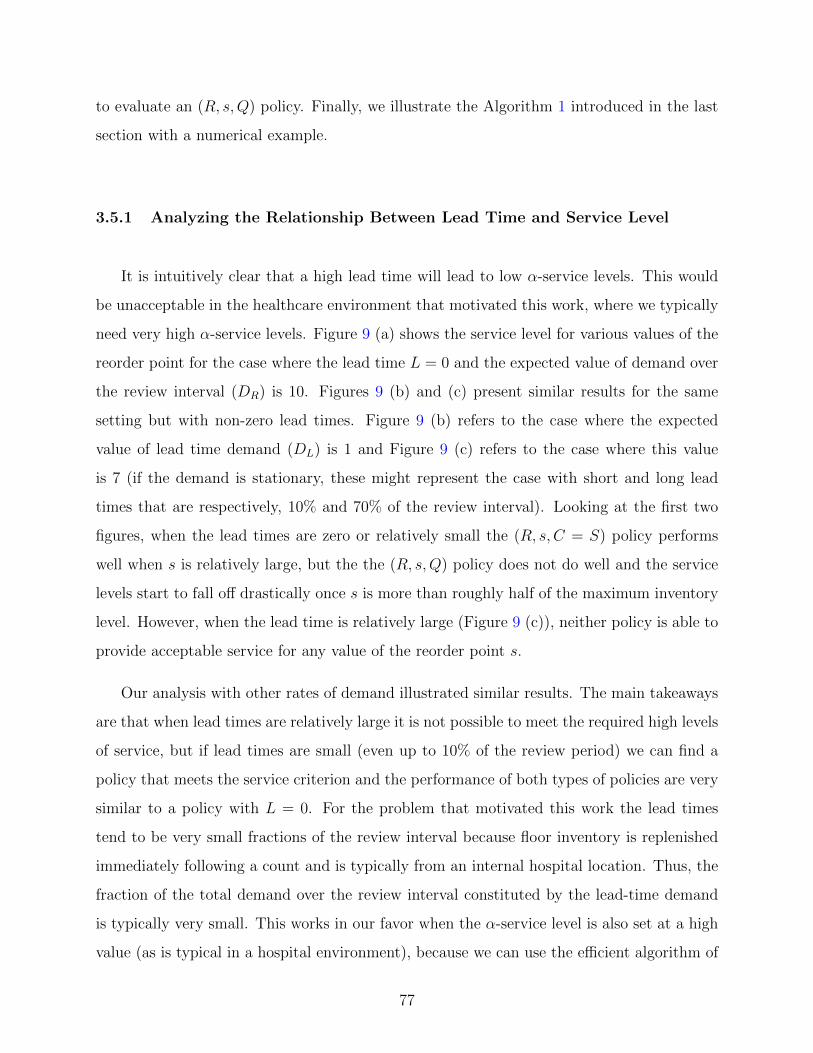
to evaluate an (R, s,Q) policy. Finally, we illustrate the Algorithm 1 introduced in the last
section with a numerical example.
3.5.1 Analyzing the Relationship Between Lead Time and Service Level
It is intuitively clear that a high lead time will lead to low α-service levels. This would
be unacceptable in the healthcare environment that motivated this work, where we typically
need very high α-service levels. Figure 9 (a) shows the service level for various values of the
reorder point for the case where the lead time L = 0 and the expected value of demand over
the review interval (DR) is 10. Figures 9 (b) and (c) present similar results for the same
setting but with non-zero lead times. Figure 9 (b) refers to the case where the expected
value of lead time demand (DL) is 1 and Figure 9 (c) refers to the case where this value
is 7 (if the demand is stationary, these might represent the case with short and long lead
times that are respectively, 10% and 70% of the review interval). Looking at the first two
figures, when the lead times are zero or relatively small the (R, s, C = S) policy performs
well when s is relatively large, but the the (R, s,Q) policy does not do well and the service
levels start to fall off drastically once s is more than roughly half of the maximum inventory
level. However, when the lead time is relatively large (Figure 9 (c)), neither policy is able to
provide acceptable service for any value of the reorder point s.
Our analysis with other rates of demand illustrated similar results. The main takeaways
are that when lead times are relatively large it is not possible to meet the required high levels
of service, but if lead times are small (even up to 10% of the review period) we can find a
policy that meets the service criterion and the performance of both types of policies are very
similar to a policy with L = 0. For the problem that motivated this work the lead times
tend to be very small fractions of the review interval because floor inventory is replenished
immediately following a count and is typically from an internal hospital location. Thus, the
fraction of the total demand over the review interval constituted by the lead-time demand
is typically very small. This works in our favor when the α-service level is also set at a high
value (as is typical in a hospital environment), because we can use the efficient algorithm of
77

Figure 9: Comparison of (R, s, S) and (R, s,Q) policies service level when D ∼ Poisson(µ = 10),and C = 15 and (a) L=0, (b)E[DL] = 1 (c)E[DL] = 7 in increasing order of reorder points
the previous section for the case where lead time is zero, when L > 0 as long as L is small.
For an (R, s, S) policy we can examine a range of values for s while for an (R, s,Q) policy
we must restrict ourselves to relatively small values of s (say less thanC
2as assumed in the
previous section).
In summary, in order to calculate the limiting probability of an inventory policy with
small lead times relative to the review interval and the α service level criterion, Propositions
4 and 5 and Algorithm 1 in the previous section can be used for the (R, s, S) policy and
Theorem 5 can be used for the (R, s,Q) policy.
78
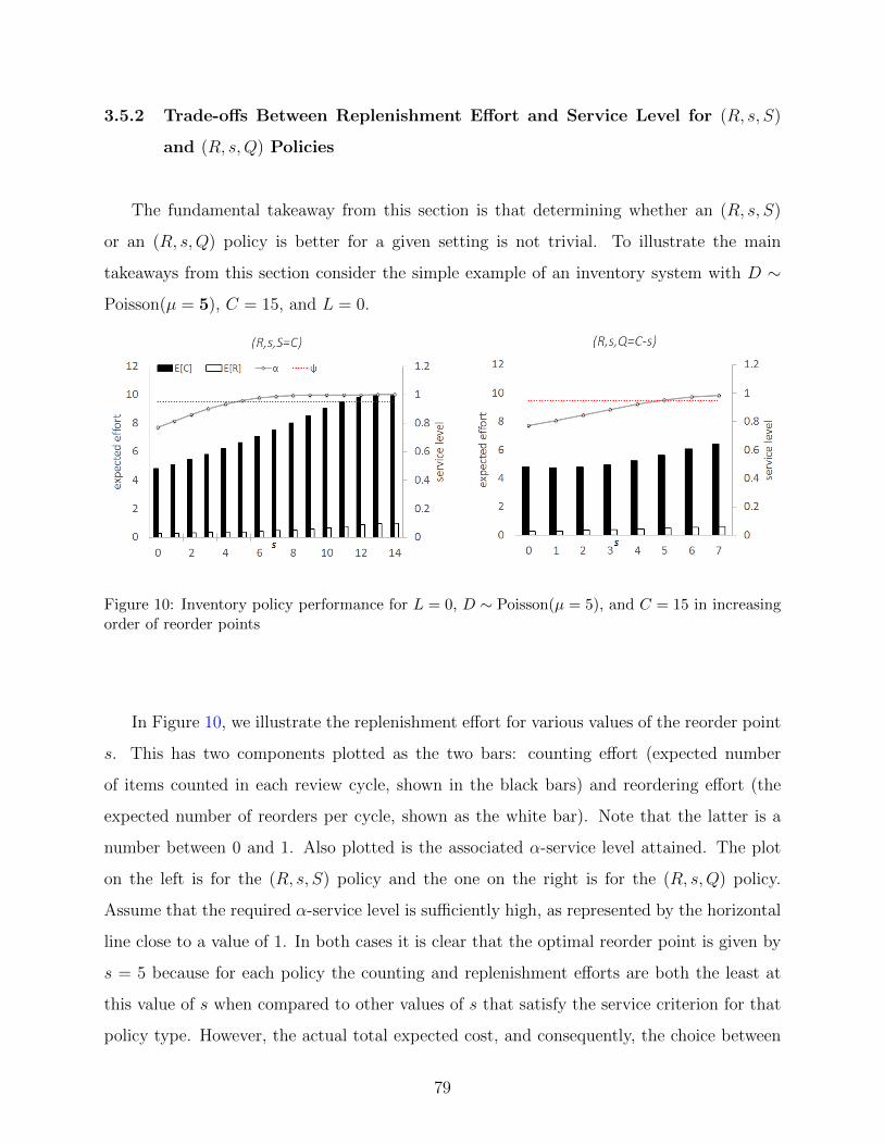
3.5.2 Trade-offs Between Replenishment Effort and Service Level for (R, s, S)
and (R, s,Q) Policies
The fundamental takeaway from this section is that determining whether an (R, s, S)
or an (R, s,Q) policy is better for a given setting is not trivial. To illustrate the main
takeaways from this section consider the simple example of an inventory system with D ∼
Poisson(µ = 5), C = 15, and L = 0.
Figure 10: Inventory policy performance for L = 0, D ∼ Poisson(µ = 5), and C = 15 in increasingorder of reorder points
In Figure 10, we illustrate the replenishment effort for various values of the reorder point
s. This has two components plotted as the two bars: counting effort (expected number
of items counted in each review cycle, shown in the black bars) and reordering effort (the
expected number of reorders per cycle, shown as the white bar). Note that the latter is a
number between 0 and 1. Also plotted is the associated α-service level attained. The plot
on the left is for the (R, s, S) policy and the one on the right is for the (R, s,Q) policy.
Assume that the required α-service level is sufficiently high, as represented by the horizontal
line close to a value of 1. In both cases it is clear that the optimal reorder point is given by
s = 5 because for each policy the counting and replenishment efforts are both the least at
this value of s when compared to other values of s that satisfy the service criterion for that
policy type. However, the actual total expected cost, and consequently, the choice between
79

an (R, s, S) and (R, s,Q) policy will depend on the specific values of the cost parameters h
and r which we defined in section 3.3 and which translate expected effort into expected cost.
Note that for the (R, s,Q) policy, as before we do not consider values of s greater thanC
2because these do not provide satisfactory service. In fact, as Figure 11 shows, it is possible
that even with the assumption that s <C
2, the (R, s,Q) policy might be infeasible.
Figure 11: Inventory policy performance for L = 0, D ∼ Poisson(µ = 10), and C = 15 in increasingorder of reorder points
In summary, there is no obvious way of picking one policy over the other in this case and
we need to study this system further to determine specific settings where one policy might
dominate the other. We will investigate some of this further in the next chapter of this
dissertation. Moreover, it is also possible that for a different value of the α-service level the
optimal values of s for the two policies might also be different from each other. In summary,
determining whether (R, s, S) or (R, s,Q) is better in the same setting is in general not
trivial and depends on the α-service level, and the values of h and r.
3.5.3 Reorder Points and Service Levels in the (R, s,Q) Policy
In this section, we focus specifically on the (R, s,Q) policy and turn our attention to the
behavior of the α service level when the reorder point increases. As Figure 9 indicates, the
80

α service level from an (R, s,Q) policy does not follow a monotonic pattern, but one thing
that appears to be consistent between these graphs and the graphs for other values of mean
demand that we studied is that with zero or small lead times, the service level reaches its
maximum around approximatelyC
2. The reason for this is that when we have a maximum
limit on what the inventory level can be, the order quantity (i.e., Q) for the (R, s,Q) policy
is not independent of s and is always fixed at Q = C − s; the closer s is to C, the smaller
the order quantity. For example, consider two cases with the same problem settings where s
equalsC
4in one and s equals
3C
4in the other (so that the corresponding order quantities Q
are given by3C
4and
C
4, respectively). The second policy orders more frequently but in small
quantities and the inventory level at the beginning of a cycle will most often be well below
its maximum value, while in the first policy the order quantities are larger and the average
inventory level at the beginning of a cycle will be closer to C. In a given problem setting,
this will lead to the first policy having better service than the second, especially when the
expected value of demand increases. The following figures show the values of the limiting
probability for each possible state (inventory level at the beginning of a cycle) corresponding
to various reorder points between 0 and C − 1. The problem setting corresponds to when
C = 15, L = 0, and we consider two cases for the mean demand:(a) µ = 5 and (b) µ = 10.
Focusing on the case where j = 0 (which corresponds to the case where at the end of the
previous cycle there was no inventory and probably resulted in a shortage), the probability
of being in this state is quite high at higher values of s, indicating that in steady state,
many cycles will experience a stock-out. In both cases this value reaches its minimum in the
vicinity ofC
2and for the case where µ = 5 we can still meet the service requirements, with
µ = 10 we cannot. Concomitantly, it can be seen that the probabilities of finishing a cycle
with large amounts on the shelf (i.e., for larger values of j) are almost zero. In summary,
when the reorder point is high with an (R, s,Q) policy the service level drops off rapidly.
As discussed in the previous section this point has been made previously in the literature
associated with the (R, s,Q) policy in settings similar to ours, and the reorder point is often
assigned a suitable upper bound (e.g., S − µ).
81

Figure 12: Inventory position analysis for L = 0, D ∼ Poisson(µ = 5), and C = 15
82

Figure 13: Inventory position analysis for L = 0, D ∼ Poisson(µ = 10), and C = 15
83

3.5.4 Computational Effort and Problem Size
In Section 3.4, we demonstrated that with L = 0 and an (R, s, S) policy we can use
Algorithm 1 to calculate the limiting probability distribution very efficiently by using a re-
cursive procedure starting with s = C and successively finding the probabilities for each
smaller value of s, without ever having to use the closed-form solution which involves the
computation of the γ values with many factorial coefficients. The procedure is easily im-
plemented within a spreadsheet and the limiting probability distribution can be calculated
in less than a second for any practical size of C. This is significant because as C increases,
the computational time for the traditional approach of solving the balance equations will
increase significantly as the size of the transition probability matrix increases. Moreover,
by using Algorithm 1, and then using Propositions 4 and 5 for the (R, s, S) policy, we are
able to calculate the γ values and use them in any setting, including with an (R, s,Q) policy
(recall that the closed forms for γ show that these values are independent of the policy and
its associated policy parameters).
Figure 14: Percentage reduction in matrix size by applying Theorem 5
Turning to the (R, s,Q) policy, via Theorem 5 we can reduce the size of the coefficient
matrix for the system of linear equations that needs to be solved to derive the limiting
84

probability distribution by at least 75% as illustrated in the following figure, where the
percentage reduction in size is plotted against values of s ∈ {0, 1, · · · , C − 1} for several
different values of C.
Without Theorem 5, if we want to calculate the limiting probability distribution for
the entire state space, we would need to solve a set of C equations simultaneously for the
(R, s,Q) policy. However, we are now able to solve only s equations simultaneously and
because by our assumption s is at most C2− 1, our reduction in matrix size will be C2s2
C2 .
3.5.5 Illustration of Algorithm 1
We illustrate the application of Algorithm 1 described at the end of Section 3.4 when
S = C = 15 and µ = 5 with Poisson demands. The table below shows the first few iterations
of the algorithms where the limiting probabilities are computed and shown for values of
s = 14, 13, 12 and 11. Initially the values of ai for i ∈ {0, 1, · · · , 14} are computed (second
column). Then we start with s = C − 1 = 14.
• In Step 1 we find the values of πj = aC−j for j = 1, 2, · · · , 15 and finally the value of
π0 = 0.00023 by subtracting the sum of these values from 1. This yields the column of
values for s = 14.
• Next, in Step 2 we move on to the column for s = 13 and find the values of πj for j = 14, 15
(the last two entries in the column) using equation (80). Thus π14 = (0.03369)/(1 −
0.00674+0.03369) = 0.03281, and π15 = (1−0.03369)∗(0.00674)/(1−0.00674+0.03369) =
0.00652.
• Then in Step 3, we find the values of πj for j = 1, 2, · · · , 13 using equation (81), e.g.,
π1 = a14 + (a13− a14)(π14 = 0.00047 + (0.00132− 0.00047) ∗ (0.03281) = 0.00050. Finally
we subtract the sum of the πj values just found from 1 to obtain π0 = 0.00024
Steps 2 and 3 are repeated to obtain π(s) for s = 12, 11, · · · , 0. With s = 12 we first find
π13, π14, π15, then π1, · · · , π12, and then π0; with s = 11 we first find π12, π13, π14, π15, then
85
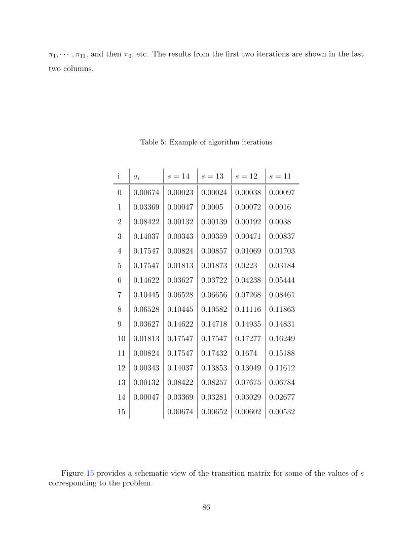
π1, · · · , π11, and then π0, etc. The results from the first two iterations are shown in the last
two columns.
Table 5: Example of algorithm iterations
i ai s = 14 s = 13 s = 12 s = 11
0 0.00674 0.00023 0.00024 0.00038 0.00097
1 0.03369 0.00047 0.0005 0.00072 0.0016
2 0.08422 0.00132 0.00139 0.00192 0.0038
3 0.14037 0.00343 0.00359 0.00471 0.00837
4 0.17547 0.00824 0.00857 0.01069 0.01703
5 0.17547 0.01813 0.01873 0.0223 0.03184
6 0.14622 0.03627 0.03722 0.04238 0.05444
7 0.10445 0.06528 0.06656 0.07268 0.08461
8 0.06528 0.10445 0.10582 0.11116 0.11863
9 0.03627 0.14622 0.14718 0.14935 0.14831
10 0.01813 0.17547 0.17547 0.17277 0.16249
11 0.00824 0.17547 0.17432 0.1674 0.15188
12 0.00343 0.14037 0.13853 0.13049 0.11612
13 0.00132 0.08422 0.08257 0.07675 0.06784
14 0.00047 0.03369 0.03281 0.03029 0.02677
15 0.00674 0.00652 0.00602 0.00532
Figure 15 provides a schematic view of the transition matrix for some of the values of scorresponding to the problem.
86

Figure 15: Schematic view of the transition matrix of the algorithm. Each color represents adifferent value.
87

3.6 CONCLUSIONS
In this chapter, we develop comprehensive discrete time Markov chain models for the
two most common periodic review systems, namely (R, s, S) and (R, s,Q) systems, that deal
with all of the aforementioned characteristics while minimizing the total expected replenish-
ment effort. We investigate the structural results and point out the tradeoffs of performance
measures of interest for different periodic review policies. We develop the transition prob-
abilities for different systems and propose an approach that only needs to calculate these
transition probabilities one time for any system regardless of its parameters; there is no need
to update these transition probabilities when changing inventory policy parameters in order
to optimize the performance measure of interest while comparing different systems. In fact,
our algorithm does not even directly use the transition probability matrix; rather, it only
needs a one-time computation of a set of simple probabilities.
We also derive closed form solutions for the limiting probability distribution of on-hand
inventory at the beginning of a review interval for several settings of interest, by using
nontrivial and novel methods. For such settings, we also propose an exact algorithm to
calculate the limiting probability distribution by locally decomposing the state space. In
this method, there is no need to explicitly solve the balance equations to find the limiting
probability distribution for any state. The derived closed form expressions and the proposed
algorithm are much easier to implement in practical applications compared to traditional
methods of solving Markov models, and the computational effort required for finding the
replenishment policy parameters is reduced tremendously. Our approach is new and has
never been used in the literature for design and analysis of the types of inventory control
systems considered here.
88
4.0 OPTIMAL SELECTION OF INVENTORY POLICIES IN A
HEALTHCARE SETTING WITH SERVICE LEVEL AND SPACE
CONSTRAINTS
4.1 INTRODUCTION
Up to 45% of a hospitals operating budget could be tied up in materials management,
which indicates that hospitals may face industry-specific inventory-related problems not ex-
perienced elsewhere (Kowalski (1991), De Vries (2011)). Higher than both the manufacturing
and distribution industries, it has been estimated that 48% of materials management costs
could be avoided with better logistical processes (Landry and Philippe 2004).
Since investment in a continuous review framework is not always cost effective, inventory
is generally reviewed at set periodic intervals (Bijvank and Vis 2012a). In practice, hospitals
tend to assign the same overall periodic inventory control policy to all or the majority of
items. This simplistic approach often leads to wasted staff effort, ineffective use of storage
space and other inefficiencies. Furthermore, the inventory policy at points of use (POU)
may cause central storage to incorrectly interpret demand consumption and interfere with
the performance of the entire supply chain.
In this chapter, we address the management of inventory for multiple non-perishable
routine use items in a healthcare setting. A PAR level approach (this was defined and
discussed in Chapter 2.3) is often used as the primary inventory control system, and this
results in operational procedures that are often inefficient and time consuming. We propose
89

a model that allows for exploration of a range of alternatives and chooses the best solution,
given space and inventory control policy constraints. The objective is to minimize the average
labor effort required to count and replenish all of the items, while providing an acceptably
high level of service (avoiding stock outs) and taking into account the available space. We
present a mixed-integer programming model for selecting the best periodic review inventory
control system for each item and the best associated storage option considering space and
item size constraints. Parameters including the dimensions of items and bins, available
inventory policies, width and depth of the shelves, and the order-up-to amount of each item,
are assumed to be given as inputs to the model. We optimize the order-up-to amount of
each item for each inventory policy separately as a preprocessing step to the model using
the results of the previous chapter. The objective is to minimize the total average effort
to replenish items over a suitable interval of time, subject to limits on the storage space
available. We consider (R, s, S), (R, s,Q), PAR level (i.e., (R, S)) and two-bin Kanban
policies (these are described further in the Section 4.3), and we jointly optimize space and
policy allocation for multiple items and optimally allocate medical items to shelves in a
storage area within a hospital by selecting the optimal inventory policy for each item along
with its corresponding operating parameters. We illustrate the model with actual data from
a Veteran’s Administration hospital in the Pittsburgh area.
The remainder of this chapter is organized as follows: Section 4.2 reviews the related
literature, Section 4.3 reviews different inventory policies considered here and their tradeoffs
while section 4.4 describes the model. Section 4.5 proposes a mixed integer programming
model while Section 4.6 presents computational test results motivated by an actual setting.
Finally, Section 4.7 provides concluding remarks.
4.2 LITERATURE REVIEW
Although most hospitals currently employ a periodic review inventory system as their
primary approach to managing inventories, seeking effective inventory management policies
90

and approaches to ensure the availability of medical and surgical supplies at the lowest
inventory control cost has consistently been a critical objective for hospital materials man-
agement and applications of operations research in health care (Little and Coughlan 2008).
Presently, in most hospital internal supply inventory management practices, nurses and staff
members use personal experience or heuristic rules to determine the timing and quantity
when replenishing inventory stock (Nicholson et al. 2004).
Multi-item inventory control gives rise to many challenging problems, and a number of
contributions have been made in the design of multi-item inventory control systems since
1960. Many of the papers in this area consider joint replenishment since ordering multiple
items independently results in a large number of small orders. Such an approach is suitable
for many systems, e.g., when we have a very large number of items, when fixed ordering
costs are very high, or when group discounts might be available. Much of the prior research
emphasizes quantitative fundamentals of inventory control systems. A huge body of litera-
ture exists on determining how to group items in such a way that all items from the same
group have the same order cycle. However, this approach is not suitable for the hospital
context since group discounts are not available and a fixed order cost is not applied to the
items considered for this study due to the fact that hospitals usually use a local warehouse.
Our main objective is to minimize the expected time that inventory staff spend to count
and replenish the items when placing orders with the hospital’s internal central warehouse
during every review period.
Other researchers have investigated multi-item inventory models incorporating other
costs or constraints. Typically, these constraints are on the budget and/or space avail-
able. Space-constrained inventory models occur naturally in the retail domain. However,
the primary retail objective is maximizing profit, which is not the case in hospitals. Much
work has also been done on optimizing a specific inventory control policy’s parameters. For
example, Golany and Lev-Er (1992) construct a multi-item, multi-period fixed quantity in-
ventory policy considering items with variable demand and determine the optimal order
quantity (Q) and reorder point (s) for each item to maximize the profit for a pharmaceutical
distributor while considering several constraints. Additionally, a wide range of optimization
91

methodologies have been used to model these problems, and due to the complexity of multi-
item inventory systems, different types of heuristic methods have also been utilized in the
literature ( Kelle et al. (2012), and Bijvank and Vis (2012a)). Much of the literature on
multi-item inventory control systems cannot easily translate to healthcare settings because
these are more focused on either very large numbers of items or very high fixed ordering
costs ( Downs et al. (2001)).
Table 6: Characteristics of the relevant literature in periodic review inventory system in hospitals
Study Demand Excess L Policy No. of SL Cap. Obj.
process demand items
Kelle et al. (2012) stoch lost int (R, s, S) multi yes yes cost
Bijvank and Vis (2012a) stoch lost frac (R, s,Q) multi yes no service
Little and Coughlan (2008) stoch back 0 (R, S) multi yes no service
Lapierre and Ruiz (2007) det back int (R, s,Q) multi yes no cost
Nicholson et al. (2004) stcoh back 0 (R, S) single no no cost
Dellaert and van de Poel (1996) stoch back 0 (R, s,Q) multi no no cost
Vincent and Ranton (1984) det back int (R, s,Q) single yes no cost
This chapter stoch lost frac (R, s, S) multi yes yes cost
(R, s,Q)
(R, S)
Kanban
Table 6 presents a summary of several important studies in the hospital inventory man-
agement literature’ this is an expanded version of the table in Bijvank and Vis (2012a) with
additional rows and columns. The key characteristics addressed in the table include whether
the demand process is deterministic (det) or stochastic (stoch); whether excess demand is
back-ordered (back) or lost; whether the lead time (L) is integral (int), fractional (frac) or
zero (0); whether the replenishment policy (Policy) is (R, s, S), (R, S), (R, s,Q), Kanban, or
(s,Q); whether there are multiple items (multi) or a single item; whether capacity limitation
92
(Cap) exist (yes) or not (no); service level limitations (SL), and the objective function (cost
or service).
In this chapter, we study a multi-item inventory control system. The inventory control
policies that we consider are the PAR level or (R, S), (R, s, S), (R, s,Q), and two-bin Kanban
systems, and we do so while imposing shelf-space constraints. To our knowledge, no prior
research has considered comparing these four inventory control policies on the aforementioned
problem.
4.3 COMPARISON OF DIFFERENT INVENTORY POLICIES IN
HOSPITALS
In its most basic form, inventory management is control over the flow of entities into
and out of a stock of different items. The tradeoffs associated with holding inventories in a
hospital are clear. More inventory means that more demand can be met and consequently,
the hospital provides better service to its patients and reduces expediting time, energy and
costs. On the other hand, holding a large volume of items means that a large amount of
space is required to store inventory. Storage space in hospitals is scattered around many
locations and usually tends to be limited; it is not uncommon to see all manner of ad hoc
storage arrangements in place. Moreover, hospital storage systems require hospital staff to
categorize, organize, count, and replenish items; these handling and administrative costs
are the most important economic factors considered in this chapter. Another problem with
holding large amounts of inventory in hospitals is that some items can have a limited shelf-
life or deteriorate over time; in this chapter we do not consider these situations. We consider
only disposable, non-perishable items within a storage area where there are typically less
than one hundred different items.
To have a good inventory control system, it is necessary to have a clear understanding of
how different inventory control policies work and are influenced by hospital characteristics.
93
There are two broad types of inventory review policies, continuous and periodic. Because
the setup cost of a monitoring system for a continuous review policy is relatively high, it
is usually utilized in hospitals mostly for critical or expensive items. In a periodic review
system, the inventory position is monitored at fixed points in time and if necessary, an order
is placed only at these times. In a hospital setting this tends to be the system of choice for
a large number of items. In particular, for the items we consider in this chapter that are
not expensive or critical, periodic review is typically used. In hospitals, the review interval
(i.e., the amount of time that elapses between two consecutive reviews of inventory in the
stockroom) is usually one day, but for some locations it could be longer and up one week for
the types of items that we consider.
The inventory policy used by most health systems defines the stocking quantity (within
a minimum and maximum value for the PAR levels) for each item based on average usage
and the desired number of days supply, e.g., an overall average of 14 days of supply for
items, and a desired fill rate of at least 98.5%. Wang et al. (2015) use a fixed order inventory
control policy model for health inventory system which uses these PAR levels as parameters
for this policy. Also, clinics sometimes set their inventory levels at a days worth of demand
with minimal safety stock (Wilson et al. (2015)).
Stressing hospitals’ need for simplicity and ease of usage is an important potential future
research area. As staff dealing with logistics activities in hospitals often do not have the same
technical background and knowledge as their counterparts in manufacturing, implementation
of sophisticated inventory systems may be difficult in hospitals. The PAR inventory method
involves a supply staff member scanning all the supplies with a hand-held scanning device
or manually counting them and entering data onto a piece of paper attached to a clip board
and possibly transcribing these into a computer system later on. The supply clerk notes any
nursing supplies that need to be replenished, or “brought up to PAR”, and then refills the
bins on a separate trip, usually later the same day. If the supply for some item runs out during
the day because of a higher usage rate than expected, the material management department
is notified in order to have an expedited delivery of the item. In a worse scenario that is not
uncommon, a clinical staff member might have to go to the central storage location and pick
94

up the item. Our model is based on ensuring that this happens with very low probability
and for very few items.
The two-bin Kanban policy has also become popular in healthcare. Here inventory is
stored in two identical bins and when the first bin is exhausted, it signals the need to reorder
a full bin. Consistent with the service level requirement of the PAR level system we set
bin capacity to s. In a continuous review context, the second bin may be viewed as reserve
stock for use during the lead-time interval, so the capacity of each bin is such that there is
enough to meet expected demand over the lead time plus some safety stock. In our periodic
review context with short lead times the capacity of each bin should be enough to meet
demand until the next review point with very high probability and thus we set this capacity
to s once again. There are numerous benefits to using the two-bin Kanban supply system
over a PAR system, including a decrease in the number of resupply trips, eliminating daily
inventory counts, and a reduction in supply shortages. A PAR system requires significant
effort for counting and replenishment and also leads to staff members taking shortcuts in
the process, which in turn leads to inaccuracies and poor service, and replenishment during
almost every review period requires significant labor. On the other hand, a Kanban system
doesn’t necessitate daily counting, eliminates “guesstimating” of supply quantities, creates
a standardized supply replenishment process, and allows for more frequent replenishment
cycles without increasing material handling costs. As a two-bin Kanban policy is much
easier to use from an operational perspective, it has been widely used for material supply in
manufacturing, and more recently the healthcare industry has been increasingly considering
the Kanban approach as an alternative to the PAR policy on the basis of efficiency, accuracy,
compliance levels, and cost savings. A recent article by Landry and Beaulieu (2013) provides
a very good chronicle of inventory systems in healthcare.
Many studies like Rosales et al. (2015) show that changing from a PAR system to a
two-bin Kanban system is an excellent move for hospitals in terms of reducing the total cost
of counting and replenishment per review cycle. However, none of these emphasize the fact
that although a two-bin Kanban system is simpler and reduces operational costs, it also has
several limitations. First, unless we can use a card separator within a single bin, we are
95
restricted to using two separate bins. With the other policies it might be possible to store
everything needed in a single bin. Thus we generally need more shelf space. Moreover, we
need to consider both bins as one item since the bins should be stored together. With this
restriction, we are less flexible when optimizing the allocation of space. Second, we generally
have more inventory; e.g., with the PAR system we have a maximum inventory of s+ 1 but
here we could have as many as 2s units (with the other two systems it would depend on the
values of S and Q). Third, this policy may not be suitable for all items. For example, si
units of a larger item i may not fit in any of the available bins. Also, we can only store 2si of
an item i with a two-bin Kanban system, and sometimes this might not be optimal because
we might want to store more of an item.
As mentioned earlier, a PAR system could result in orders for an item being placed in
every review cycle (especially items with high usage levels). Therefore in the context of
medical inventory, an alternative and more general approach is to use a system that allows a
range of desired inventory values. Here the inventory level of an item i is never allowed to fall
below some minimum value (LBi) or exceed some maximum value (UBi). The value of LBi
is based on some minimum level of service (fill-rate or probability of not stocking out) that
is to be provided over the review interval (although, based on our experience in numerous
hospital settings, this is done based on clinician experience as opposed to any rigorous
statistical methodology). The value of UBi is set based on some conservative estimate of
the maximum possible demand for the item over the review period, or possibly, based on
space considerations. When these values are specified and a PAR system is in use, the PAR
level must be chosen to be within this desired range. It is common in some hospital settings
to use the terms minimum PAR and maximum PAR to denote these desired minimum and
maximum levels, even when the actual system in use is not a PAR system. We adopt the
more general notation of LBi and UBi since the terms minimum PAR and maximum PAR
are not meaningful when used with inventory control strategies that do not follow a PAR
system. Moreover, all four policies we consider can be implemented within the constraints
of LBi and UBi. Specifically, we consider
96

• (R, s, S | S = C) policy: LBi ≤ s < C ≤ UBi
• (R, s,Q | Q = C − s) policy: LBi ≤ s < C ≤ UBi
• (R, S | S = C) policy: LBi ≤ C − 1 < C ≤ UBi
• (R, s,Q | s = Q = bC2c) policy: LBi ≤ C
2< C ≤ UBi
Note that in order to be stable and have a reasonable service level, the reorder point should
satisfy the following two conditions, s < C − µ and s < C2
, for an (R, s,Q) policy where
µ is the expected value of the stochastic demand for all policies. Consequently, (R, s, S) or
Kanban policies might not be even feasible for an item because of this condition regardless of
the desired service level. In the following section, we describe the model for choosing which
inventory control policy to use for an item and compare some of the structural properties of
the different policies.
4.4 MODEL AND ALGORITHM DEVELOPMENTS
We begin with several modeling assumptions. First, we assume the items are stored on
standard steel shelving units and the dimension of each shelving unit is H ×W ×D. There
are a total of N items, where item i is a rectangular solid of dimensions hi × wi × di and
there are B different bin types where bin type l can store nil units of item i. We assume
that the amount of time to count an item (h) is the same for all items, as are the amounts
of time to replenish each item (r). We summarize our assumptions as follows:
• space in patient-unit storage rooms is limited
• shelving units have standard rectangular shapes
• all items are stored in bins
• there is a limited set of bin sizes
• a single bin size is used for any item
• only one item type is allowed to be stored in a lane of bins
97

• there is no bin stacking
• two equal-sized bins (or card-separated bin sections) are used if a Kanban policy is used
• the summation of the widths of all the bins used for a given item is less than the width
of a shelving unit
Note that, in this chapter we use the same inventory control settings and notation as in the
previous chapter. For ease of notation, we will henceforth index and refer to the (R, s, S),
(R, s,Q), PAR, and Kanban policies as Policies 1, 2, 3, and 4, respectively. We summarize
the sets and indices that we use in the following table.
Table 7: Summary of sets and indices used for the models
Set/Index Explanation
i index for item type, i ∈ I, where I = {1, 2, · · · , N}
j index for policy type, j ∈ Ji where Ji ⊆ {1, 2, 3, 4}
l index for bin type, l ∈ {1, 2, · · · , B}
Kji set of possible values for the maximum inventory level as-
sociated with item i when it uses policy j, i.e., Kji =
{LBi, · · · , UBi}
k the value of the maximum inventory level considered for a
policy j to use with with item i; k ∈ Kji ,
Next, we redefine equations (3.8), (3.9), and (3.10) from the previous chapter in order to
make them be a function of the policy, and its related parameters. In general there are two
parameters: s, which represents the reorder point as before and k, which is the value of
C ∈ {LBi, · · · , UBi}
98

Table 8: Parameters for deriving objective function coefficients
Parameter Explanation
Hji (s, k) expected counting effort: the expected number of units counted per review
period for item i with policy j and corresponding parameters s and k
Rji (s, k) expected reorder effort: the expected number of reorders per review period for
item i with policy j and corresponding parameters s and k
T ji (s, k) total expected replenishment effort: the total expected effort to control the
inventory at each review point for item i with policy j and corresponding
parameters s and k
αji (s, k) service level: the probability of not being out-of-stock during a review period
for item i with policy j and corresponding parameters s and k
∆ji (k) feasible reorder point set: a set of all feasible reorder points for item i with
policy j and corresponding parameter k where the system is stable and meets
the service criterion
ϕ service level threshold: the lower bound for the α-service level
We define T ji (s, k) as
T ji (s, k) = hHji (s, k) + rRj
i (s, k), (4.1)
and ∆ji (C)for ∀j ∈ {1, 2, 3, 4} separately as,
∆1i (k) = {s | 0 ≤ s < k − 1, α1
i (s, k) ≥ ϕ}, ∀i, (4.2)
∆2i (k) = {s | 0 ≤ s < min{k − µ, k
2}, α2
i (s, k) ≥ ϕ}, ∀i, (4.3)
∆3i (k) = {s | s = k − 1, α3
i (k − 1, k) ≥ ϕ}, ∀i, (4.4)
∆4i (k) = {s | s =
k
2, α4
i (k
2, k) ≥ ϕ}, ∀i. (4.5)
If ∆ji (k) = ∅, then the corresponding policy j is infeasible for item i and will not be
contained in Ji. For a given item i we consider each policy j ∈ Ji and each value of parameter
k ∈ Kji for the maximum inventory level, and find the optimal value of the reorder point
99

(s∗) that minimizes total expected replenishment cost. We denote the corresponding total
expected cost in one review period by f ji (k), i.e., this is the cost if item i uses policy j with
maximum inventory level C = k. Thus
f ji (k) = min{T ji (s, k) | s ∈ ∆ji (k)}, (4.6)
It is obvious that the reorder point for the PAR and Kanban policies are fixed once k is
specified; therefore, we do not need(4.6) to optimize the reorder point. As a result, assuming
that s = k − 1 ∈ ∆3i (k) and s = k
2∈ ∆4
i (k) are feasible for the PAR and Kanban policies
respectively, we will have,
f 3i (k) = T 3
i (k − 1, k), ∀i (4.7)
f 4i (k) = T 4
i (bk2c, k), ∀i (4.8)
Finally, we also select the best policy j∗ for a given item i and a given maximum inventory
level C = k and specify the corresponding cost via
j∗ ∈ arg minj{fji (k)} (4.9)
fi(k) = f j∗
i (k) (4.10)
Let us define s∗i (j, k) as the optimal reorder point for item i with policy j when we use
parameter value k for the maximum inventory level permitted (C). In the following corollary,
we investigate the behavior of parameters of interest in the (R, s, S) policy (i.e., with j = 1)
Corollary 2. The following statements are true for the (R, s, S) policy with item i,
1. For any k, Rji (k), Hj
i (k), and αji (k), are increasing in s,
2. s∗i (1, k) = arg min {s|αji (k) > ϕ}.
100

Proof. Consider an item i and two (R, s, S) policies with different reorder points si(1, k) and
s′i(1, k) for a given value of S = k, where si(1, k) < s′i(1, k). Let us denote by X and Y
(respectively) the on-hand inventory levels at the beginning of some arbitrary review cycle
for these two policies. If X and Y are both less than si(1, k), or greater than s′i(1, k) then the
decision is the same for both cases, and the inventory levels at the beginning of the next cycle
will differ by the same amount as they currently do. However, when si(1, k) < X, Y ≤ s′i(1, k)
then we need to reorder for the system that has reorder point s′i(1, k) but not for the one that
has si(1, k). In particular, we are adding an amount k − Y > 0, which makes the on-hand
inventory level higher for the second system at the beginning of the next review cycle. In
addition, we are also reordering more frequently because of the reorder point being higher.
So, the counting and replenishment efforts are both higher with reorder point s′i(1, k) and
this proves clause (1). Clause (2) follows directly from the results of clause (1).
The following corollary indicates that for the same value k for the maximum inventory
level allowed, the PAR system has higher counting and replenishment effort but provides
better service.
Corollary 3. The following statements are true when comparing the (R, s, S) and PAR
policies,
1. H1i (s, k) ≤ H3
i (k − 1, k),
2. R1i (s, k) ≤ R3
i (k − 1, k),
3. α1i (s, k) ≤ α3
i (k − 1, k).
Proof. Recognizing that the PAR policy is equivalent to the (R, s, S = k) policy with s =
k − 1, the result follows directly from Corollary 2
Using the results of Corollary 2 and after running several examples and observing the
behavior of the optimal reorder point for high service levels, we propose the following two
algorithms (one for each of the (R, s, S), and (R, s,Q) policies) to calculate the optimal re-
order point with a service constraint. This is more efficient for finding f ji (k) than calculating
101

T ji (s, k) for all s ∈ ∆ji (k) for the (R, s, S) and (R, s,Q) policies. The algorithms are simple
search methods that begin with an initial guess of E[D] for the value of s. We then search
among successively higher values if this is not feasible, and if it is not feasible, then we search
among successively lower values for the smallest feasible value.
Algorithm 2. For an item i and parameter value k, the optimal reorder point, s∗i (1, k) for
an (R, s, S) policy may be found as follows.
1. We start with s = E[D], and calculate the α-service level; if α1i (s, k) ≥ ϕ, then go to the
next step, otherwise go to step 3.
2. If s = 0, then s∗i (1, k) = 0 and go to step 5, otherwise reduce s by 1, and calculate the
α-service level. If α1i (s, k) ≥ ϕ, repeat this step, otherwise s∗i (1, s) = s+ 1 and go to step
5.
3. If s = k, then go to the next step; otherwise, increase s by 1, and calculate the α-service
level; If α1i (s, k) ≥ ϕ, s∗i (1, k) = s and go to step 5, otherwise, repeat this step.
4. Report that the problem is infeasible with the current α-service level and go to the next
step.
5. Terminate the algorithm.
Algorithm 3. For an item i and parameter value k the optimal reorder point, s∗i (2, k) for
an (R, s,Q) policy may be found as follows:
1. We start with s = E[D],and calculate the α-service level; if α2i (s, k) ≥ ϕ, then go to the
next step, otherwise go to step 3.
2. If s = 0, then s∗i (2, k) = 0 and go to step 5, otherwise reduce s by 1, and calculate the
α-service level; If α2i (s, k) ≥ ϕ repeat this step, otherwise s∗i (2, k) = s+ 1 and go to step
5.
3. If s ≥ min{k − E[X], bk2c} go to step 4, otherwise, increase s by 1, and calculate the
α-service level; If α2i (s, k) ≥ ϕ, s∗i (2, k) = s and go to step 5, otherwise, repeat this step.
4. Report that the problem is infeasible with the current α-service level and go to the next
step.
102

5. Terminate the algorithm.
We tested 100 different instances for these two algorithms and also enumerated across
all possible values of s. In all of the instances, these two algorithms are able to either find
the optimal s or determine if the problems is infeasible.
The following table contains a summary of the notation that we have either already used
or wish to use in order to derive the parameters of interest for our mathematical programming
model, which will choose the best combination of policies across our set of items. Up until
this point, we have focused on deriving the objective function coefficients and now, we discuss
how to assign the optimal bin size to item i and policy j with corresponding parameter value
k.
Table 9: Summary of parameters needed for the models
Parameters Explanation
N number of item types
B number of bin types
A number of shelving units
nil capacity of bin l to store item i
hl × wl × dl dimensions of bin l
H ×W ×D dimensions of available shelf space (all shelving units) with corresponding volume
V
vji (k) required volume to store item i using policy j with its associated parameter value
k
wji (k) required width to store item i using policy j with its associated parameter value
k
hji (k) required height to store item i using policy j with its associated parameter value
k
103

Now for every item and its corresponding feasible policy set (i.e., Ji), we iteratively check
different numbers of possible bins in this set for every bin type, i.e., {⌊LBi
nil
⌋, · · · ,
⌈UBi
nil
⌉}. For
different permutations of bin type and possible numbers of that bin, we test for each item
and policy to see at first whether it is feasible and second, to determine the optimal k
for each permutation of bin type and number. We update Kji accordingly and remove those
parameter values for the maximum storage level that are not optimal for a given bin size and
possible bin number. Then, we review the results for each bin size and compare the results
across different policies for that size with dominated policies being removed. Therefore, for
each bin size and value of k only one policy can be assigned: the space requirement is the
same and the policy with the least cost will be assigned to that specific item for that specific
bin type and associated number of bins. Next, we review the different bin sizes and if a larger
bin results in higher cost, then the corresponding parameter value associated with that bin
is also removed from Kji because it is dominated. Finally, based on the components of Kj
i ,
we update wji (k) ,hji (k),and vji (k).
Now, let Γik = j∗ from (4.9) denote the optimal policy for item i when we use corre-
sponding parameter value k. In the next section, we will use this definition to create the
shelf space allocation model. Because we don’t need the index j (we can find the optimal j
via (4.9) if we know its corresponding parameter value k), we drop the index j and for ease
of notation, we redefine vi(k) = vΓik
i (k), hi(k) = hΓiki (k), and wi(k) = w
Γik
i (k).
Note that in the worst case scenario, we end up with a maximum value of⌈UBi
nil
⌉−⌊LBi
nil
⌋+1
for the size of the parameter value set Kji for each combination of item and policy. As this
process is very straightforward, we do not write a formal algorithm for it and treat it as a
preprocessing procedure. In the next section, we define the space allocation models based
on the derivation within this section.
104
4.5 OPTIMAL ALLOCATION MODELS BASED ON REPLENISHMENT
EFFORT
In this section we define a two-dimensional level bin packing (2LBP) model. We formulate
a model that minimizes the total expected counting and replenishment time subject to
constraints on storage area, item and bin dimensions and available inventory control policies.
The objective of the model is to select exactly one candidate for each item i along with its
associated value of k, as well as to decide on how the item should be assigned to the available
shelf space. We assume that all required units of an item are on a single shelf in order to
facilitate easy access to the item when it is needed. Shelves in shelving units at POU can
only have discrete height values as the number of bin sizes is limited. We assume that each
shelf can have a different height but that it is a multiple of some base unit height h (i.e.,
the possible heights are h, 2h, 3h, · · · ). Using this idea we divide a shelving unit into a set
of shelves that are arranged vertically with a height that is a multiple of h. We also update
the values of hi(k) and H correspondingly. Let us define the index l ∈ {1, · · · , H}.
In the next page, we redefine MIP1 for this problem, and call it the 2LBP model. The
objective function (4.11) represents the total expected cost of counting and replenishment.
Constraint set (4.12) ensures that the width constraint for each shelf is not violated. Con-
straint set (4.13) ensures that the relationships between the x and z variables are correct,
and constraint set (4.14) ensures that each item is stored with exactly one policy with one
associated parameter value. Constraint set (4.15) ensures that no item on any lower shelf is
tall enough to cause it to intrude into the space occupied by a higher shelf.
Decision Variables
xlik: = 1 if item i with parameter k is located on a shelf at height position l; 0 otherwise
(binary)
yl: = 1 if a shelf is located at position l; 0 otherwise (binary)
105

Model 2LBP
min∑i
∑k
fi(k) zik, (4.11)
subject to:∑i
∑k
wi(k)xlik ≤ Wyl ∀l, (4.12)
zik ≤∑l
xlik ∀i, k (4.13)
∑k
zik = 1 ∀i, (4.14)
yl + xrik ≤ 1 ∀l, i, k,∀r ∈ {max{1, l − hi(k) + 1}, · · · , l − 1}, (4.15)
zik ∈ {0, 1}, ∀i, k, xlik ∈ {0, 1}, ∀i, k, l. (4.16)
4.6 COMPUTATIONAL ANALYSIS
In this section, we have four different subsections. First, we compare (R, s, S) and
(R, s,Q) policies and examine their tradeoffs which leads to a conjecture and discussion
about that conjecture. Second, we perform sensitivity analysis for the service level across all
four policies and show how the optimal reorder point changes when we change the service
level. Then, using real data from a healthcare setting we illustrate the behavior of a hybrid
inventory control policy when we change the available storage space. We also provide some
guidelines and insights based on this real example. Finally, we generate data to test the
performance of our model and to consider the tradeoffs between different policies across
different inventory policy parameter settings.
4.6.1 Trade-offs Between (R, s, S) and (R, s,Q)
In this section, we compare different policies regarding their expected counting or order-
ing efforts, and the service level. In Conjecture 1, we compare (R, s, S) and (R, s,Q) policies
106
based on the computational results from the inventory system that we consider.
Conjecture 1. Given i, s and k, the following statements are true for comparing (R, s, S)
and (R, s,Q) policies when lead time is insignificant,
1. H1i (s, k) ≥ H2
i (s, k),
2. R1i (s, k) ≤ R2
i (s, k),
3. α1i (s, k) ≥ α2
i (s, k).
The order quantity (i.e., Q) for an (R, s,Q) policy is fixed (i.e., Q(j = 2) = k − s),
regardless of the on-hand inventory level (i.e., equation (3.1)) at the reorder point. Therefore
only when inventory on-hand equals s will our order quantity be k−s and we might be at our
maximum capacity, k, when the order arrives. But in an (R, s, S) policy, Q(j = 1) = k − i,
and no matter how much inventory is on-hand at the reorder point, there is a chance that we
will order and hence that we will be at our maximum capacity, k, when the order arrives. As
we noted while proving Corollary 2, in an (R, s, S) policy the expected inventory on-hand at
the beginning of any review interval is more than in an (R, s,Q) policy. We will demonstrate
our conjecture above with several examples.
The first four sets of figures below compare for a single item the counting and reordering
effort associated with the two policies for two different demand rates of µ = 5 and µ = 10,
with (a) zero lead time and (b) a positive but relatively small lead time where the mean lead
time demand is either 10% (µ = 10) or 20% (µ = 5) of the mean demand over the review
interval. There are several takeaways. First, as per our conjecture, the counting effort for the
(R, s, S) policy is always higher while the reorder effect is always lower when compared to
the (R, s,Q) policy when we have a constraint on the maximum inventory allowed. Second,
the behavior of the cost elements in the presence of a positive but small lead time is quite
similar to that with zero lead time. Third, the (R, s,Q) policy is often unable to provide the
required service level when demand rates are high.
107

Figure 16: Comparison of (R, s, S) and (R, s,Q) policies (a) expected counting effort, (b) expectedreordering effort, and (c) α-service level when D ∼ Poisson(µ = 5), L = 0, and C = 15 in increasingorder of reorder points.
Figure 17: Comparison of (R, s, S) and (R, s,Q) policies (a) expected counting effort, (b) expectedreordering effort, and (c) service level when D ∼ Poisson(µ = 10), L = 0, and C = 15 in increasingorder of reorder points.
108

Figure 18: Comparison of (R, s, S) and (R, s,Q) policies (a) expected counting effort, (b) expectedreordering effort, and (c) service level when D ∼ Poisson(µ = 5), E[DL] = 1, and C = 15 inincreasing order of reorder points.
Figure 19: Comparison of (R, s, S) and (R, s,Q) policies (a) expected counting effort, (b) expectedreordering effort, and (c) service level when D ∼ Poisson(µ = 10), E[DL] = 1, and C = 15 inincreasing order of reorder points.
109

In order to further clarify the logic behind our conjecture, consider the limiting probabil-
ity of being in a particular state j, where 0 ≤ j ≤ C = 15 for a given value of s. Suppose we
compute this probability for every possible value of s and then sum these values up. While
this sum has no physical interpretation, larger values for a particular j would imply that
across all possible reorder points, that value of j is more likely for the state of the system
(the inventory level at the beginning of a review interval). In the figures below we plot these
values as a stacked sum for (R, s, S) and (R, s,Q) for various values of j. Figures 20 and
21 correspond to two different values of the expected demand of 5 and 10, respectively. As
both figures show, when we consider larger values of j, the sum of the limiting probabilities
across all reorder points with the (R, s, S) policy is generally higher when compared to the
sum for the (R, s,Q) policy. This implies that an (R, s, S) policy will generally have higher
inventory levels when counting is done and this results in higher counting effort. However, it
will also provide better service because of the higher inventory level. We also notice a pattern
with the (R, s, S) policy. The sum of these limiting probabilities for a given j appears to
be directly related to Pr(D = C − j), the probability that the demand is equal to C − j.
We also plot this probability for each j for the (R, s, S) policy in the figures below. In this
policy, the highest limiting probabilities are close to values of C − E[D] corresponding to
which Pr(D = C − j) is at a maximum as well.
Figure 20: Limiting probabilities for different on-hand inventory levels; D ∼ Poisson(µ = 5)
110

Figure 21: Limiting probabilities for different on-hand inventory levels; D ∼ Poisson(µ = 10)
4.6.2 Sensitivity Analysis for Service Level Across All Policies
In this section, we change the threshold for the service level and investigate the effect of
this change on the optimal reorder point. In Figures 22 (R, s, S) and 23 (R, s,Q), we study
the behavior of the reorder point as the threshold for the service level increases, for two
different values of expected demand and three different values of the maximum inventory
level allowed. Note that if the policy is infeasible based on the threshold, we remove the point
for that value of the threshold from the graph. We did not perform this particular analysis
for PAR and Kanban policies because the reorder point is fixed with these two policies. We
may summarize our takeaways from these plots as follows:
• the optimal reorder point with the (R, s, S) policy is non-decreasing in the service thresh-
old, as long as it is not infeasible
• the behavior of the optimal reorder point depends on the expected demand as well as
the maximum allowable inventory level
• our algorithm to determine the value ofs has better performance for the (R, s, S) policy
but in both, it is able to find the optimal value
• the behavior of the optimal value for the (R, s,Q) policy is inconsistent because it depends
on r and h
111
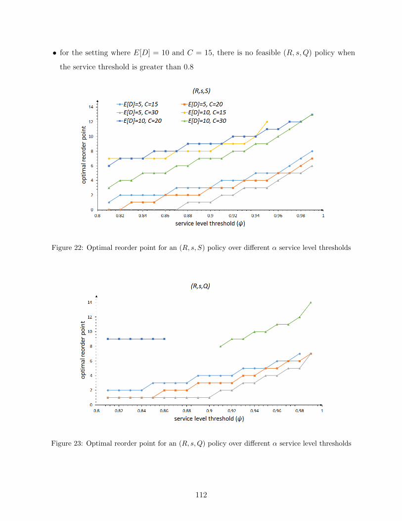
• for the setting where E[D] = 10 and C = 15, there is no feasible (R, s,Q) policy when
the service threshold is greater than 0.8
Figure 22: Optimal reorder point for an (R, s, S) policy over different α service level thresholds
Figure 23: Optimal reorder point for an (R, s,Q) policy over different α service level thresholds
112

For the PAR policy and Kanban policy the service level results are as follows for the
aforementioned settings:
Table 10: Summary of service level for PAR and Kanban policy
Setting PAR Kanban
E[D] = 5, C = 14 0.9998 0.9763
E[D] = 5, C = 20 1.0000 0.9991
E[D] = 5, C = 30 1.0000 1.0000
E[D] = 10, C = 14 0.9165 infeasible
E[D] = 10, C = 20 0.9984 0.8068
E[D] = 10, C = 30 1.0000 0.9960
instead of C = 15, we consider C = 14 for the Kanban policy.
4.6.3 Optimal Allocation Based on Changing Available Storage Space
In this section, we illustrate the proposed IP formulation using actual data from a hos-
pital. We select a subset of 100 items with diverse characteristics, stored in a stockroom
with multiple standard steel shelving units each with height 70 in., width 30 in. and depth
21 in. There are 8 different bin types corresponding to all combinations of height = 4 or
8 inches, depth = 6 or 12 inches and width = 12 or 24 inches. The review interval is one
week long and the optimal reorder point is computed for each item i using a 99th percentile
service level.
In Table 11, we report the optimal value for the proposed IP model across several in-
stances. We use the maximum number of shelves as a key problem size factor for all instances
to see what happens when we limit space, assuming that the fixed cost per replenishment
is fifty times the unit counting cost (r = 50, h = 1). The average daily replenishment and
counting effort for each item is obtained by using the limiting probabilities derived by the
113
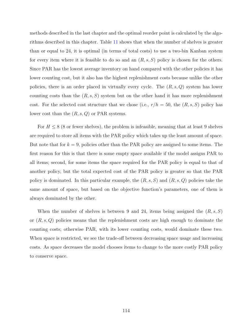
methods described in the last chapter and the optimal reorder point is calculated by the algo-
rithms described in this chapter. Table 11 shows that when the number of shelves is greater
than or equal to 24, it is optimal (in terms of total costs) to use a two-bin Kanban system
for every item where it is feasible to do so and an (R, s, S) policy is chosen for the others.
Since PAR has the lowest average inventory on hand compared with the other policies it has
lower counting cost, but it also has the highest replenishment costs because unlike the other
policies, there is an order placed in virtually every cycle. The (R, s,Q) system has lower
counting costs than the (R, s, S) system but on the other hand it has more replenishment
cost. For the selected cost structure that we chose (i.e., r/h = 50, the (R, s, S) policy has
lower cost than the (R, s,Q) or PAR systems.
For H ≤ 8 (8 or fewer shelves), the problem is infeasible, meaning that at least 9 shelves
are required to store all items with the PAR policy which takes up the least amount of space.
But note that for k = 9, policies other than the PAR policy are assigned to some items. The
first reason for this is that there is some empty space available if the model assigns PAR to
all items; second, for some items the space required for the PAR policy is equal to that of
another policy, but the total expected cost of the PAR policy is greater so that the PAR
policy is dominated. In this particular example, the (R, s, S) and (R, s,Q) policies take the
same amount of space, but based on the objective function’s parameters, one of them is
always dominated by the other.
When the number of shelves is between 9 and 24, items being assigned the (R, s, S)
or (R, s,Q) policies means that the replenishment costs are high enough to dominate the
counting costs; otherwise PAR, with its lower counting costs, would dominate these two.
When space is restricted, we see the trade-off between decreasing space usage and increasing
costs. As space decreases the model chooses items to change to the more costly PAR policy
to conserve space.
114
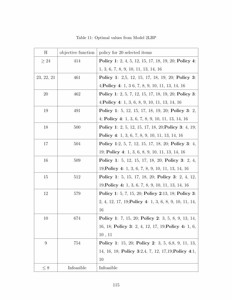
Table 11: Optimal values from Model 2LBP
H objective function policy for 20 selected items
≥ 24 414 Policy 1: 2, 4, 5, 12, 15, 17, 18, 19, 20; Policy 4:
1, 3, 6, 7, 8, 9, 10, 11, 13, 14, 16
23, 22, 21 461 Policy 1: 2,5, 12, 15, 17, 18, 19, 20; Policy 3:
4;Policy 4: 1, 3 6, 7, 8, 9, 10, 11, 13, 14, 16
20 462 Policy 1: 2, 5, 7, 12, 15, 17, 18, 19, 20; Policy 3:
4;Policy 4: 1, 3, 6, 8, 9, 10, 11, 13, 14, 16
19 491 Policy 1: 5, 12, 15, 17, 18, 19, 20; Policy 3: 2,
4; Policy 4: 1, 3, 6, 7, 8, 9, 10, 11, 13, 14, 16
18 500 Policy 1: 2, 5, 12, 15, 17, 18, 20;Policy 3: 4, 19;
Policy 4: 1, 3, 6, 7, 8, 9, 10, 11, 13, 14, 16
17 504 Policy 1:2, 5, 7, 12, 15, 17, 18, 20; Policy 3: 4,
19; Policy 4: 1, 3, 6, 8, 9, 10, 11, 13, 14, 16
16 509 Policy 1: 5, 12, 15, 17, 18, 20; Policy 3: 2, 4,
19;Policy 4: 1, 3, 6, 7, 8, 9, 10, 11, 13, 14, 16
15 512 Policy 1: 5, 15, 17, 18, 20; Policy 3: 2, 4, 12,
19;Policy 4: 1, 3, 6, 7, 8, 9, 10, 11, 13, 14, 16
12 579 Policy 1: 5, 7, 15, 20; Policy 2:13, 18; Policy 3:
2, 4, 12, 17, 19;Policy 4: 1, 3, 6, 8, 9, 10, 11, 14,
16
10 674 Policy 1: 7, 15, 20; Policy 2: 3, 5, 8, 9, 13, 14,
16, 18; Policy 3: 2, 4, 12, 17, 19;Policy 4: 1, 6,
10 , 11
9 754 Policy 1: 15, 20; Policy 2: 3, 5, 6,8, 9, 11, 13,
14, 16, 18; Policy 3:2,4, 7, 12, 17,19;Policy 4:1,
10
≤ 8 Infeasible Infeasible
115
Figure 24: Optimal policy based on the number of shelves and item characteristics for a sample of20 items
In figure 24, we show the characteristics of sample items from a prosthetics POU for a
VA hospital in Pittsburgh. We multiply demand for an item by the volume of that item
and then order the items in decreasing order of this measure. In the following, we discuss
some general guidelines and rules of thumb for hospitals by considering the results of this
section and based on studying the transition between different policies for items with different
characteristics and in different settings. By different characteristics, we mean demand (low,
high), size (small, large) and by different settings, we mean replenishment and reordering
effort and required service level. We summarize our findings as follows:
• (R, s, S) policy
– when item is small and demand is high
– when replenishment cost is high
– when service level is high
116
• (R, s,Q) policy
– when item is small and demand is low
– when counting cost is high
– when service level is not extremely high
• PAR policy
– when item is large and demand is high
– when replenishment cost is low
– when service level is extremely high
• Kanban policy
– when item is small and demand is low
– when counting cost is very high
– when service level is not extremely high
Note that guidelines stated above are very general and not universally true; for a partic-
ular combination of items that need to be stored, a hospital would need to run our model to
arrive at the best set of policies and the associated storage scheme.
4.6.4 Tradeoffs Between Different Policies Considering Different Inventory Con-
trol Parameter Settings
In this section we investigate the tradeoffs between the different inventory policies and
test the performance of our model. To do this, we randomly generated expected item demand
and associated bin size data for a set of 185 items. The data is depicted in Figure 25,
with expected demands ranging between 1 and 50 as displayed along the x-axis, and the
corresponding width of the bin (which can contain an amount equal to the expected demand)
as displayed along the y-axis. We assume that the height of each bin is the same and that we
have 20 different bin widths ranging between 1 and 20 units. This set of items was then used
with our model in three different settings with the following combinations of the required α
service level and values for the costs of counting (r) and replenishment (h):
117

1. α = 0.95, r = 50, h = 1
2. α = 0.95, r = 1, h = 1
3. α = 0.9, r = 1, h = 1
For each setting we ran our algorithm with different numbers of available shelves, up to
a maximum of 30 shelves.
Figure 25: Randomly generated item bin size and demand data
The run time varies from a few seconds to one minute. Figures 26 (a), (b), and (c) display
for the above settings (respectively), the number of items (out of 185) that are assigned a
particular policy for each given value of the number of shelves available for storage. With
fewer than 10 shelves, the problem is infeasible and the optimal value remains unchanged
when we go beyond 23 shelves. Figures 27 (a), (b) and (c) that follow provide for the three
settings (respectively) a display of how the maximum inventory of the 185 items in storage
with the optimum policy is distributed among the items for different numbers of available
shelves. The items are divided into groups having maximum inventory levels equal to 2,
3, 4, 5 or 6 times the expected demand rate at the optimum, and the number of items in
each group is depicted. Finally, Figures 28 (a), (b) and (c) display for the three settings
(respectively), the total cost across all 185 items when we select the best policy for each
item, plotted as a function of the number of shelves available for storage.
118

Figure 26: Distribution of inventory systems when the number of shelves increases for (a) setting1 (b) setting 2 (c) setting 3
119

Figure 27: Distribution of the maximum inventory on-hand when the number of shelves increasesfor (a) setting 1 (b) setting 2 (c) setting 3
120
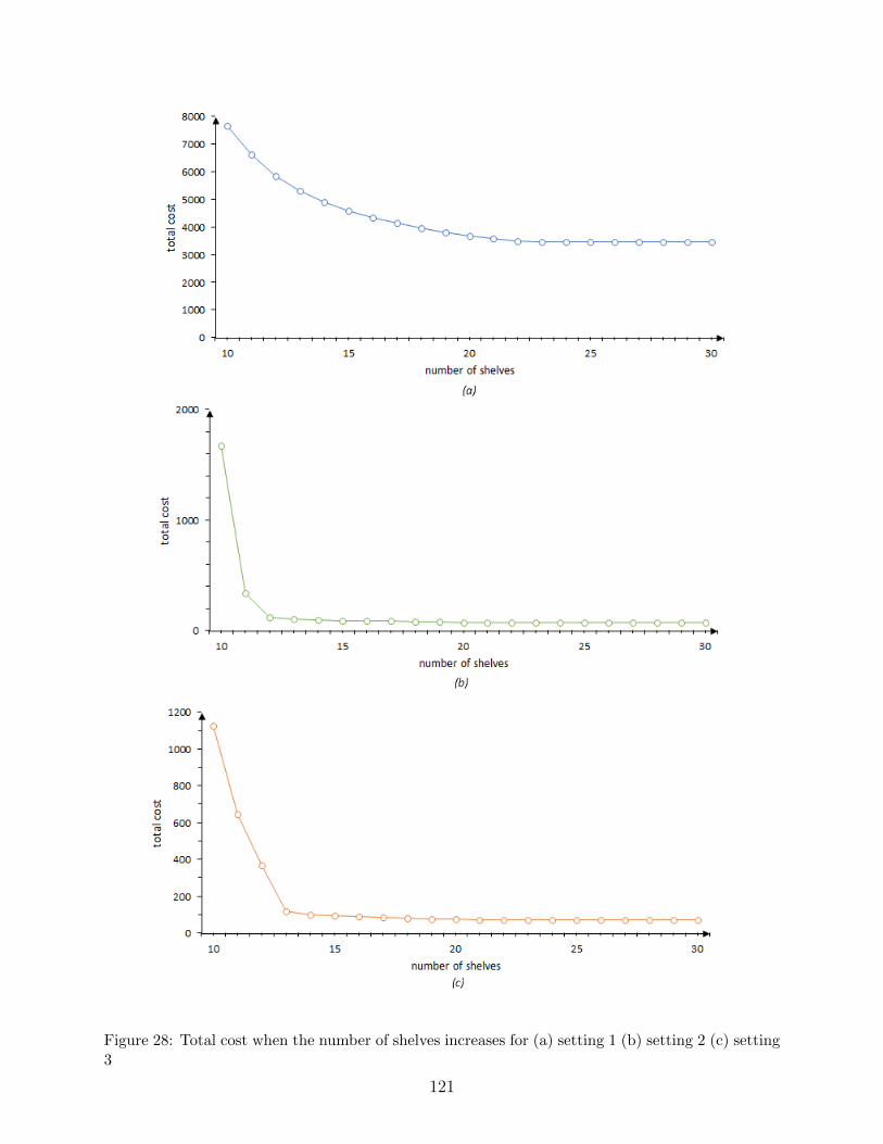
Figure 28: Total cost when the number of shelves increases for (a) setting 1 (b) setting 2 (c) setting3
121

We summarize takeaways as the following:
• In the first setting, only the Kanban and (R, s, S) policies are chosen and when we
decrease the reorder costs relative to counting cost (in setting 1 it is 50 times the counting
cost and in settings 2 and 3 it is equal to the counting cost), the PAR policy is also chosen
for a few items. This is because the frequent ordering with the PAR policy does not add
as much to the cost any more. The (R, s,Q) policy is very rarely selected for an item.
• Sometimes, even when sufficient space is available for an item with the Kanban policy
(using the bin size that was assigned to the item), the (R, s, S) policy is chosen. This
happens because an (R, s, S) policy can have less frequent ordering than a Kanban policy
and if the reorder costs are relatively high, the former policy can be more attractive than
the latter one.
• As the optimal policy differs for items with different bin widths it is not trivial to deter-
mine how the final policy for an item is changed when we change the ratior
h.
• The change in total cost when we increase the number of shelves is monotone non-
increasing.
• The change in total cost when we change the ratior
his not linear.
• In general, Kanban and (R, s, S) are dominating the other policies.
• We observe in setting 3 that when the required α service level decreases, the (R, s,Q)
policy is used instead of the Kanban policy. Recall that we assume that the optimal
reorder point in the (R, s,Q) policy is less thanC
2which reduces both the counting effort
and the reordering effort compared to when the reorder point equalsC
2. Therefore, we
can conclude that in those cases when the (R, s,Q) policy is selected instead of a Kanban
policy, these reduction are large enough that the reordering cost with the Kanban policy
is greater than the sum of the counting and reordering costs with the (R, s,Q) policy.
• Because the counting cost is considered to be zero in the Kanban policy, the Kanban
policy dominates the (R, s,Q) policy most of the time.
• Generally, the total cost decreases when the ratior
hdecreases (Figure 28 (a) vs. Figures
28 (b) and (c)). However, the behavior of the cost curve is somewhat different for the
two cases. In both cases attaining the minimum possible cost for each of the settings
122

requires 23 shelves. However, with the lowerr
hvalue the cost drops quite rapidly as we
start increasing the number of shelves from the minimum required value of 10, and we are
able get quite close to this minimum cost with relatively few shelves (around 14). Whenr
his high the decrease in costs as the number of shelves increases is much more gradual.
This is because whenr
h= 1 the counting cost is very high relative to the reordering
cost, so that the Kanban policy quickly becomes very attractive (this is also validated by
Figures 26 (b) and (c)) and so as soon as there is shelf space available the items choose
the Kanban policy and quickly approach the minimum cost policy. Generally, the total
cost decreases when the α service level decreases (Figure 28 (b) vs. Figure 28 (c)).
• Generally, the maximum inventory on-hand decreases when the α service level decreases
(Figures 27 (b) vs. (c)).
• Generally, the maximum inventory on-hand decreases when the reordering cost decreases
(Figure 27 (a) vs. Figures 27 (b) and (c)).
4.7 SUMMARY AND CONCLUSIONS
In this chapter, we consider a specific storage area or stockroom at a POU location that
is restocked from a central location within the hospital. The major cost drivers are the
effort to monitor and replenish inventory for the items in the storage location as opposed
to the holding cost, which is incurred irrespective of where in the system the item is stored.
We study a multi-item system with shelf space constraints, where any of several different
inventory policies such as (R, s, S), (R, s,Q), PAR, and Kanban can be used for an item.
We assume a fractional lead time, stochastic demand, and a service level constraint as well
as space restrictions. We propose a shelf space allocation approach using a 2LBP approach.
The results indicate that the more shelves we have the more we tend to use a Kanban policy
and the less shelving space we have we utilize an (R, s, S) policy and perhaps the PAR
system.
123

5.0 CONCLUSIONS AND FUTURE WORK
This dissertation addresses inventory control and logistics challenges related to pharma-
ceuticals as well as medical and surgical supplies within a hospital and how to optimally solve
these problems to minimize hospital staff effort. Despite the existence of well-documented
evidence on the benefits of the introduction of good supply chain management practices
and the resulting cost reduction, the health care sector has been extremely slow to embrace
these practices. Regardless of having some rather unique characteristics, only a few studies
have addressed the question of how the design and implementation of inventory systems in a
health service setting takes place. This dissertation is dedicated to improving the efficiency
of health care by optimizing space allocation in healthcare facilities that are typically very
space constrained, choosing the best inventory control system for different items and improv-
ing the allocation of health care resources to reduce medication errors and staff effort needed
to manage inventory. All of the chapters of this dissertation demonstrate the importance of
providing resources by anticipating needs and making adjustments as needs change.
Decentralized ADCs can be an integral component of distribution systems within phar-
macy departments across the hospital. There are significant challenges associated with man-
aging ADC inventory optimally while minimizing labor and capital resources. The role of
enhanced inventory control functionality is not fully defined for these devices. The aim of
one chapter of this dissertation is to improve ADC inventory management by leveraging
dynamic inventory parameters. To do so, we optimally determine what items and how many
of each should be stored in decentralized ADCs within a patient unit, while simultaneously
determining the storage layout within the ADC. The approach considers each item’s demand
124
and inventory control parameters, as well as its size. There are two main goals associated
with our approach. First, when supplies are not immediately available, it typically means
that a nurse, medical assistant or other clinician needs to retrieve out-of-stock items from
central storage. This is expensive and disruptive, and our goal is to minimize such oc-
currences. Second, we also aim to minimize possible errors that might arise from storing
look-alike and/or sound-alike (LASA) medications next to each other. We use a novel MIP
approach to maximize the benefits from stocking items in decentralized ADCs located at
POUs, as measured by expected reductions in time spent by clinical personnel in manag-
ing expedited deliveries. We investigate both position-free and position-based paradigms to
allocate shelf space optimally and design appropriate layouts that reduce the likelihood of
potentially serious human errors from selecting the wrong medication.
In the first model, we focus on only assigning items to an ADC in an efficient way with re-
gard to the space required. We also propose valid inequalities, upper-bounds, and continuous
relaxations to facilitate solving large, practically sized instances. Based on computational
tests using actual data, these refinements can reduce the run time to well under 10% of the
time for the base model and thereby allow for large, real-world instances to be readily solved.
We show that our approach is better than other methods from the literature with regard to
computational time.
In the second model, we also aim to minimize possible errors that might arise from storing
similar medications next to each other. To do so, we present a grid-based position paradigm
to control errors due to storing medications with similar names and/or packaging next to
each other. The model reduces selection errors by designing a layout that assigns medications
with high similarity ratings to storage locations that are sufficiently nonadjacent within an
ADC. Our results indicate that simplistic space allocation and inventory management could
result in about twice as much work for medical staff while still leaving unused space in the
ADC, while the second (position-based) model decreases risks associated with medication
errors by at least 38% for the data set we considered.
125

Next, we develop discrete time Markov chain models of inventory control systems which
are used at POUs. These systems are characterized by limited storage capacity, stochastic
demand, periodic reviews with fractional lead times, expedited delivery when stocking out,
and very high service level requirements. We have derived closed form solutions and propose
an exact algorithm to calculate the limiting probability distribution by locally decomposing
the state space. We decompose the transition probabilities into independent parts, and then
we solve each part locally to derive product form solutions. As there is no precise algorithm
in the literature to derive such closed form solutions, probability theorists still refer to this
approach as a ”bag of tricks” and note that the application of this method is an art form
that is derived by trial and error. A major contribution of this chapter is that we derive
exact closed-form solutions for an (R, s, S) policy and we reduce the number of equations at
least in half for an (R, s,Q) policy by locally decomposing the state space for the specific
class of inventory systems considered herein.
Also for the (R, s, S) policy, by using the derived closed form structure, we propose an
algorithm which recursively solves the problem from s = C−1 to get the limiting probability
distribution for every possible value of the reorder point. This algorithm is very easy to
implement and can even be implemented in a spreadsheet. By using this algorithm, not
only do we not need to update the transition probability matrix required to calculate the
inventory control policy each time we consider a new reorder point, but we also don’t need
to solve a set of simultaneous linear equations to get the results for the limiting probability
distribution. In fact, using this method, there is no need to even calculate coefficients in
the form of factorials (product-form) and the computational time is negligible for a problem
of any realistic size. For an (R, s,Q) policy, we reduce the number of equations that need
to be solved simultaneously to a maximum of s < C2
equations. This contribution leads
to a reduction in the number of equations of at least 50% and the size of the transition
matrix reduces by at least 75%. In the numerical results, we also show that even when
lead time is greater than zero the results from when the lead time equals zero are a very
good approximation, as long as the lead time is small. In summary, the main contribution
of this section of the dissertation the derivation of closed-form expressions for the limiting
126

distribution, and an algorithm that is very easy to implement in practical applications and
entails far less effort than solving steady-state equations for Markov models. The overall
computational effort required for finding the optimal replenishment policy parameters is
thus significantly reduced.
Finally, in the last chapter we investigate the tradeoffs between standard inventory con-
trol policies used at POUs such as PAR, (R,s, S), (R,s, Q), and two-bin Kanban systems. We
optimally allocate medical and surgical items to shelves in a storage area within a hospital by
selecting the optimal inventory policy for each item along with its corresponding operating
parameters. In practice, hospitals tend to assign the same overall inventory control policy to
all or the majority of the items. This simplistic approach often leads to wasted staff effort
and ineffective policies. Our objective is to pick policies for items that reduce replenishment
and counting effort by hospital staff.
To do so, by using the results of the previous chapter, we propose two algorithms to find
the optimal reorder point for the different items. We show that the optimal reorder point
for an (R, s, S) policy doesn’t depend on the counting and reordering unit effort. Using this
result, we propose an efficient algorithm that can find the optimal reorder point for an item in
a few steps. By solving several instances for the (R, s,Q) policy and looking at the patterns
in those instances, we propose another algorithm to find the (R, s,Q) optimal reorder point.
The algorithm for (R, s,Q) can also find the reorder point in a reasonable number of steps.
Finally, by using a 2-dimensional level bin packing approach, we simultaneously select the
inventory policy for each item along with its corresponding operating parameters as well as
assign those items to shelving units at POU locations. We illustrate the model with actual
data from a healthcare setting and offer some practical insights and guidelines on how to
choose a hybrid inventory system based on demand and system characteristics.
Also, there are several directions for future research in this area. We now explain poten-
tial future work and extensions for the material in Chapters 2, 3 and 4. For the first chapter,
an initial thought is to examine further ways to reduce the computation times for our formu-
lations. It may be possible to insert additional valid inequalities or to reformulate portions
127

of the model. Second, one could explore creating heuristics that can be easily applied. The
effectiveness of the heuristics can be compared with the results from the optimization model.
Third, one could also consider analyzing the problem for various performance metrics while
explicitly considering different inventory policies that might be used for the items (e.g.,
(R, s, S), (R, s,Q) or two-bin Kanban). Fourth, one could also extend this to develop a joint
location-allocation formulation that examines the issue of how to optimally locate a given
set of ADCs within different patient units or floors of a hospital, along with the storage
and configuration of each, so as to minimize overall staff effort. A fifth idea relates to the
formulation of MIP1, where one possible extension might be reformulating the model as a
robust optimization model. Finally, for MIP2 one can consider other approaches for defining
the error coefficient and then comparing the results for this new definition with respect to
the optimal values found using the original and new definitions.
For the work in Chapter 3 , the first set of extensions would continue to address the
zero lead time case described in this work but focus on the (R, s,Q) system. One extension
would entail finding an algorithm to reduce the number of balance equations when s ≥ C2
for this policy. This in turn could lead to the development of a more efficient algorithm,
similar to the one used for the (R, s, S) policy, for determining the corresponding policy
parameters. A second and more challenging set of extensions would consider non-zero lead
times. Corresponding transition matrices would need to be defined for these cases (for both
(R, s, S) and (R, s,Q) policies) and these would then be used to develop structural results
for both classes of inventory systems along the lines of what was done in for zero lead times
in this work. These results could then be used to develop suitable algorithms for the case
with non-zero lead times as well, similar to what we did in Chapter 4. would focus more on
t Finally, further study is required to determine the threshold values of non-zero lead time,
up to which we can still reasonably approximate the results by using the results for the case
where lead time equals zero.
For the last chapter, the first possible extension is to investigate finding closed form
solutions for the optimal reorder point for both the (R, s, S) and (R, s,Q) policies. A second
extension would be to conduct extensive numerical data analyses using different data sets
128

form different hospitals to compare different policies with different item sizes and reorder
and counting coefficients in order to draw more general conclusions regarding when to use
which type of inventory management policy.
129

APPENDIX A
LM MODEL ADOPTION TO MIP1
We describe an adaptation of the LM Model for our problem. In a preprocessing step,
items are first arranged based on decreasing order of their heights (with ties being broken
arbitrarily). Then, each lane of an item is considered as a possible shelf position (i.e.,
there are M =∑
i∈I ui possible shelf positions). Item i can be located on shelves 1 to
Ai =∑ui
s=1 us, while shelf s can store items with indices in the range Bs to N , where
βs = {min k : 1 ≤ k ≤ N, αk ≥ s,∀s ∈ (1, · · · , M)}. Instead of x and y, we define two sets
of new decision variables (x, y). Other decision variables and all parameters remain the
same.
Decision Variables
xis: number of (additional) lanes of item i located on shelf s (integer)
ys: = 1 if shelf s is used (binary)
130
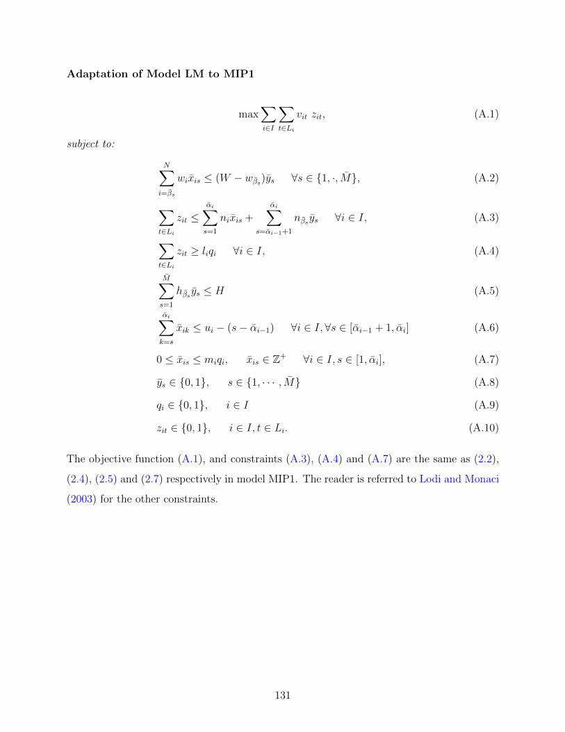
Adaptation of Model LM to MIP1
max∑i∈I
∑t∈Li
vit zit, (A.1)
subject to:
N∑i=βs
wixis ≤ (W − wβs)ys ∀s ∈ {1, ·, M}, (A.2)
∑t∈Li
zit ≤αi∑s=1
nixis +
αi∑s=αi−1+1
nβs ys ∀i ∈ I, (A.3)
∑t∈Li
zit ≥ liqi ∀i ∈ I, (A.4)
M∑s=1
hβs ys ≤ H (A.5)
αi∑k=s
xik ≤ ui − (s− αi−1) ∀i ∈ I,∀s ∈ [αi−1 + 1, αi] (A.6)
0 ≤ xis ≤ miqi, xis ∈ Z+ ∀i ∈ I, s ∈ [1, αi], (A.7)
ys ∈ {0, 1}, s ∈ {1, · · · , M} (A.8)
qi ∈ {0, 1}, i ∈ I (A.9)
zit ∈ {0, 1}, i ∈ I, t ∈ Li. (A.10)
The objective function (A.1), and constraints (A.3), (A.4) and (A.7) are the same as (2.2),
(2.4), (2.5) and (2.7) respectively in model MIP1. The reader is referred to Lodi and Monaci
(2003) for the other constraints.
131

APPENDIX B
EXAMPLE OF (R, S, S) AND (R, S,Q) PROBABILITY TRANSITION
MATRICES
The following matrices are for (R, s = 4, S = 12) and (R, s = 4, Q = 8) respectively.
Note that C = 12 for both policies.
P (R, 4, 12) =
b0 a11 a10 a9 a8 a7 a6 a5 a4 a3 a2 a1 a0
b0 a11 a10 a9 a8 a7 a6 a5 a4 a3 a2 a1 a0
b0 a11 a10 a9 a8 a7 a6 a5 a4 a3 a2 a1 a0
b0 a11 a10 a9 a8 a7 a6 a5 a4 a3 a2 a1 a0
b0 a11 a10 a9 a8 a7 a6 a5 a4 a3 a2 a1 a0
b7 a4 a3 a2 a1 a0 0 0 0 0 0 0 0
b6 a5 a4 a3 a2 a1 a0 0 0 0 0 0 0
b5 a6 a5 a4 a3 a2 a1 a0 0 0 0 0 0
b4 a7 a6 a5 a4 a3 a2 a1 a0 0 0 0 0
b3 a8 a7 a6 a5 a4 a3 a2 a1 a0 0 0 0
b2 a9 a8 a7 a6 a5 a4 a3 a2 a1 a0 0 0
b1 a10 a9 a8 a7 a6 a5 a4 a3 a2 a1 a0 0
b0 a11 a10 a9 a8 a7 a6 a5 a4 a3 a2 a1 a0
132
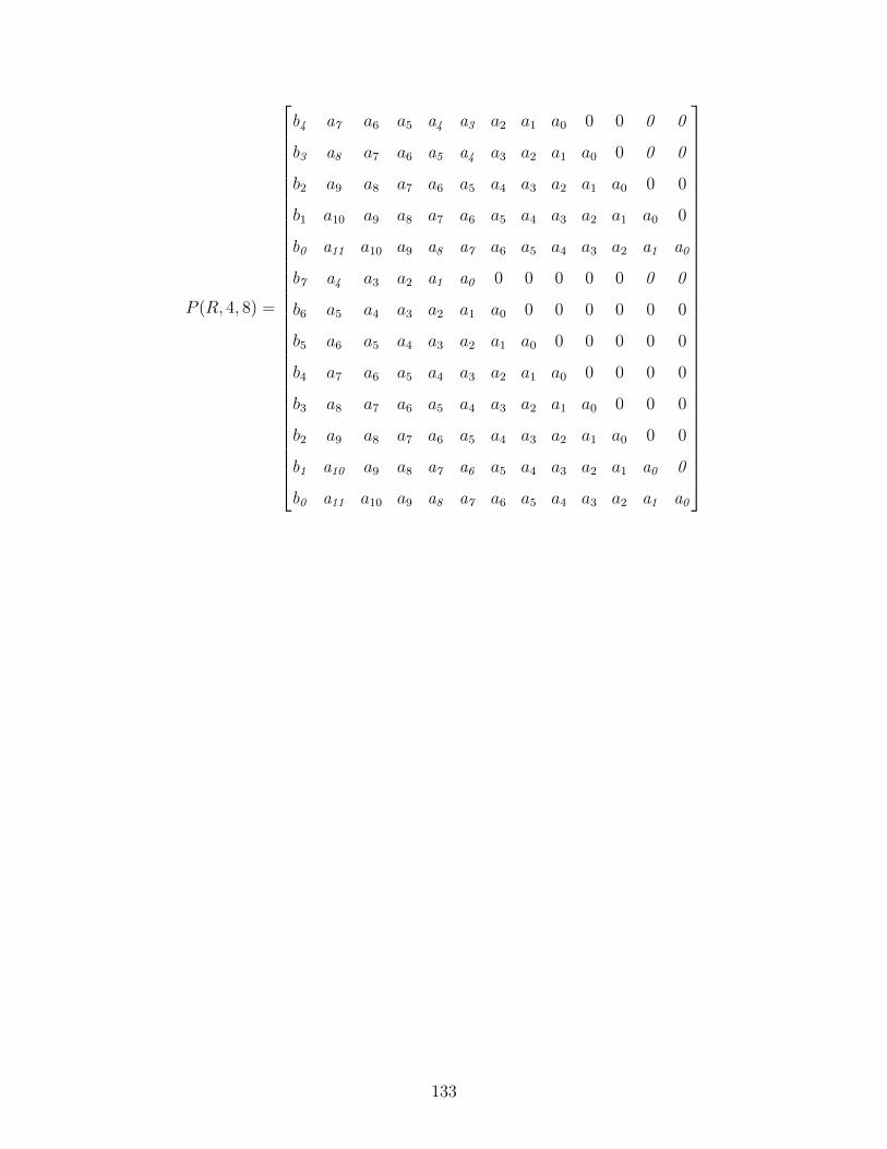
P (R, 4, 8) =
b4 a7 a6 a5 a4 a3 a2 a1 a0 0 0 0 0
b3 a8 a7 a6 a5 a4 a3 a2 a1 a0 0 0 0
b2 a9 a8 a7 a6 a5 a4 a3 a2 a1 a0 0 0
b1 a10 a9 a8 a7 a6 a5 a4 a3 a2 a1 a0 0
b0 a11 a10 a9 a8 a7 a6 a5 a4 a3 a2 a1 a0
b7 a4 a3 a2 a1 a0 0 0 0 0 0 0 0
b6 a5 a4 a3 a2 a1 a0 0 0 0 0 0 0
b5 a6 a5 a4 a3 a2 a1 a0 0 0 0 0 0
b4 a7 a6 a5 a4 a3 a2 a1 a0 0 0 0 0
b3 a8 a7 a6 a5 a4 a3 a2 a1 a0 0 0 0
b2 a9 a8 a7 a6 a5 a4 a3 a2 a1 a0 0 0
b1 a10 a9 a8 a7 a6 a5 a4 a3 a2 a1 a0 0
b0 a11 a10 a9 a8 a7 a6 a5 a4 a3 a2 a1 a0
133
BIBLIOGRAPHY
Arpit, M. and M. Laura (2015). Using lean principles to optimize adc stock. Pharmacy purchasingand product 12 (5), 4.
Bijvank, M. and S. G. Johansen (2012). Periodic review lost-sales inventory models with compoundpoisson demand and constant lead times of any length. European Journal of OperationalResearch 220 (1), 106–114.
Bijvank, M. and I. F. Vis (2012a). Inventory control for point-of-use locations in hospitals. Journalof the Operational Research Society 63 (4), 497–510.
Bijvank, M. and I. F. Vis (2012b). Lost-sales inventory systems with a service level criterion.European Journal of Operational Research 220 (3), 610–618.
Bolch, G., S. Greiner, H. de Meer, and K. S. Trivedi (2006). Queueing networks and Markov chains:modeling and performance evaluation with computer science applications. John Wiley & Sons.
Cheung, K.-C., M. L. Bouvy, and P. A. De Smet (2009). Medication errors: the importance of safedispensing. British journal of clinical pharmacology 67 (6), 676–680.
De Vries, J. (2011). The shaping of inventory systems in health services: A stakeholder analysis.International Journal of Production Economics 133 (1), 60–69.
Dellaert, N. and E. van de Poel (1996). Global inventory control in an academic hospital. Interna-tional Journal of Production Economics 46, 277–284.
Dolan, E. D. and J. J. More (2002). Benchmarking optimization software with performance profiles.Mathematical programming 91 (2), 201–213.
Downs, B., R. Metters, and J. Semple (2001). Managing inventory with multiple products, lags indelivery, resource constraints, and lost sales: A mathematical programming approach. Man-agement Science 47 (3), 464–479.
Duclos, L. K. (1993). Hospital inventory management for emergency demand. International Journalof Purchasing and Materials Management 29 (3), 29–38.
Ferenc, J. (2010). Time well spent? assessing nursing-supply chain activities. Materials managementin health care 19 (2), 12–16.
134

Furini, F. and E. Malaguti (2013). Models for the two-dimensional two-stage cutting stock problemwith multiple stock size. Computers & Operations Research 40 (8), 1953–1962.
Geismar, H. N., M. Dawande, B. Murthi, and C. Sriskandarajah (2015). Maximizing revenuethrough two-dimensional shelf-space allocation. Production and Operations Management .
Golany, B. and A. Lev-Er (1992). Comparative analysis of multi-item joint replenishment inventorymodels. The International Journal Of Production Research 30 (8), 1791–1801.
Goldberg, D. A., D. A. Katz-Rogozhnikov, Y. Lu, M. Sharma, and M. S. Squillante (2016). Asymp-totic optimality of constant-order policies for lost sales inventory models with large lead times.Mathematics of Operations Research.
Grissinger, M. (2012). Safeguards for using and designing automated dispensing cabinets. Pharmacyand Therapeutics 37 (9), 490.
Hall, R. W. (2012). Handbook of Healthcare System Scheduling. Springer.
Handfield, R. (2007). New trends in medical dispensing technology: reducing the total cost ofpatient care, white paper, supply chain resource cooperative. Ph. D. thesis, North CarolinaState University.
Hansen, P. and H. Heinsbroek (1979). Product selection and space allocation in supermarkets.European journal of operational research 3 (6), 474–484.
Harchol-Balter, M. (2013). Performance Modeling and Design of Computer Systems: QueueingTheory in Action. Cambridge University Press.
Holdford, D. A. and T. R. Brown (2010). Introduction to hospital and health-system pharmacypractice. ASHP.
Horsham (PA): Institute for Safe Medication Practices (2009). Ismp medication safety self-assessment for automated dispensing cabinets. http://www.ismp.org/selfassessments/
ADC/survey.pdf.
Hyland, S., C. Koczmara, B. Salsman, E. L. S. Musing, and J. Greenall (2007). Optimizing theuse of automated dispensing cabinets. The Canadian Journal of Hospital Pharmacy 60 (5).
ISMP (2008). Guidance on the interdisciplinary safe use of automated dispensing cabinets. http://www.ismp.org/Tools/guidelines/ADC_Guidelines_Final.pdf.
Janakiraman, G. and J. A. Muckstadt (2004). Periodic review inventory control with lost salesand fractional lead times. School of Operations Research and Industrial Engineering, CornellUniversity .
Jylanki, J. (2010). A thousand ways to pack the bin-a practical approach to two-dimensionalrectangle bin packing. retrived from http://clb. demon. fi/files/RectangleBinPack. pdf .
135

Kapalka, B. A., K. Katircioglu, and M. L. Puterman (1999). Retail inventory control with lost sales,service constraints, and fractional lead times. Production and operations management 8 (4),393–408.
Kelle, P., J. Woosley, and H. Schneider (2012). Pharmaceutical supply chain specifics and inventorysolutions for a hospital case. Operations Research for Health Care 1 (2), 54–63.
Kowalski, J. C. (1991). Inventory to go: can stockless deliver efficiency? Healthcare financialmanagement: journal of the Healthcare Financial Management Association 45 (11), 21–2.
Landry, S. and M. Beaulieu (2013). The challenges of hospital supply chain management, fromcentral stores to nursing units. In Handbook of Healthcare Operations Management, pp. 465–482. Springer.
Landry, S. and R. Philippe (2004). How logistics can service healthcare. In Supply Chain Forum:an International Journal, Volume 5, pp. 24–30. Taylor & Francis.
Lapierre, S. D. and A. B. Ruiz (2007). Scheduling logistic activities to improve hospital supplysystems. Computers & Operations Research 34 (3), 624–641.
Levi, R., G. Janakiraman, and M. Nagarajan (2008). A 2-approximation algorithm for stochasticinventory control models with lost sales. Mathematics of Operations Research 33 (2), 351–374.
Little, J. and B. Coughlan (2008). Optimal inventory policy within hospital space constraints.Health Care Management Science 11 (2), 177–183.
Lodi, A. and M. Monaci (2003). Integer linear programming models for 2-staged two-dimensionalknapsack problems. Mathematical Programming 94 (2-3), 257–278.
McCoy, L. K. (2005). Look-alike, sound-alike drugs review: include look-alike packaging as anadditional safety check. Joint Commission Journal on Quality and Patient Safety 31 (1),47–53.
McKone-Sweet, K. E., P. Hamilton, and S. B. Willis (2005). The ailing healthcare supply chain: aprescription for change. Journal of Supply Chain Management 41 (1), 4–17.
Nachtmann, H. and E. A. Pohl (2009). The state of healthcare logistics. Cost and quality improve-ment opportunities.
Nicholson, L., A. J. Vakharia, and S. Selcuk Erenguc (2004). Outsourcing inventory manage-ment decisions in healthcare: Models and application. European Journal of Operational Re-search 154 (1), 271–290.
Oh, H. C., J. A. Wong, and M. C. Tan (2014). Enhancement of patient and staff experienceat outpatient pharmacy via optimization of drug–shelf reallocation. Operations Research forHealth Care 3 (1), 15–21.
Opolon, D. C. (2010). Improving product availability in hospitals: the role of inventory inaccuracies.Ph. D. thesis, Massachusetts Institute of Technology.
136

PA-PSRS (2005). Pennsylvania patient safety authority problems associated with automated dis-pensing cabinets. 2 (3), 21–23.
Pazour, J. A. and R. D. Meller (2012). A multiple-drawer medication layout problem in automateddispensing cabinets. Health care management science 15 (4), 339–354.
Pedersen, C. A., P. J. Schneider, and D. J. Scheckelhoff (2012). Ashp national survey of pharmacypractice in hospital settings: dispensing and administration-2011. American Journal of Health-System Pharmacy 69 (9), 768.
Rosales, C. R., M. Magazine, and U. Rao (2014). Point-of-use hybrid inventory policy for hospitals.Decision Sciences 45 (5), 913–937.
Rosales, C. R., M. Magazine, and U. Rao (2015). The 2bin system for controlling medical suppliesat point-of-use. European Journal of Operational Research 243 (1), 271–280.
Schneider, H. (1978). Methods for determining the re-order point of an (s, s) ordering policy whena service level is specified. Journal of the Operational Research Society 29 (12), 1181–193.
Sherali, H. D. and J. C. Smith (2001). Improving discrete model representations via symmetryconsiderations. Management Science 47 (10), 1396–1407.
Stock, G. N., K. L. McFadden, and C. R. Gowen (2007). Organizational culture, critical suc-cess factors, and the reduction of hospital errors. International Journal of Production Eco-nomics 106 (2), 368–392.
Subramanian, S. (2013). Managing space in forward pick areas of warehouses for small parts.
Uthayakumar, R. and S. Priyan (2013). Pharmaceutical supply chain and inventory managementstrategies: Optimization for a pharmaceutical company and a hospital. Operations Researchfor Health Care 2 (3), 52–64.
Vincent, V. and M. Ranton (1984). Hospital pharmacy inventory management: economic orderquantity model with space limitation. Hospital materiel management quarterly 5 (3), 82.
Volland, J., A. Fugener, J. Schoenfelder, and J. O. Brunner (2015). Material logistics in hospitals:A literature review. Available at SSRN 2611917 .
Walter, R., N. Boysen, and A. Scholl (2013). The discrete forward–reserve problem–allocating space,selecting products, and area sizing in forward order picking. European Journal of OperationalResearch 229 (3), 585–594.
Wang, Y., S. W. Wallace, B. Shen, and T.-M. Choi (2015). Service supply chain management: Areview of operational models. European Journal of Operational Research 247 (3), 685–698.
Wascher, G., H. Haußner, and H. Schumann (2007). An improved typology of cutting and packingproblems. European Journal of Operational Research 183 (3), 1109–1130.
Wilson, K. J., R. Hodge, and D. Bivens (2015). Reducing stockouts in a cancer centers ambulatorycare clinics. Engineering Management Journal 27 (3), 99–108.
137

Zhao, Y. Q. and S. X. Li (1997). Stationary probabilities of markov chains with upper hessenbergtransition matrices. INFOR: Information Systems and Operational Research 35 (3), 197–207.
Arpit, M. and M. Laura (2015). Using lean principles to optimize adc stock. Pharmacy purchasingand product 12 (5), 4.
Bijvank, M. and S. G. Johansen (2012). Periodic review lost-sales inventory models with compoundpoisson demand and constant lead times of any length. European Journal of OperationalResearch 220 (1), 106–114.
Bijvank, M. and I. F. Vis (2012a). Inventory control for point-of-use locations in hospitals. Journalof the Operational Research Society 63 (4), 497–510.
Bijvank, M. and I. F. Vis (2012b). Lost-sales inventory systems with a service level criterion.European Journal of Operational Research 220 (3), 610–618.
Bolch, G., S. Greiner, H. de Meer, and K. S. Trivedi (2006). Queueing networks and Markov chains:modeling and performance evaluation with computer science applications. John Wiley & Sons.
Cheung, K.-C., M. L. Bouvy, and P. A. De Smet (2009). Medication errors: the importance of safedispensing. British journal of clinical pharmacology 67 (6), 676–680.
De Vries, J. (2011). The shaping of inventory systems in health services: A stakeholder analysis.International Journal of Production Economics 133 (1), 60–69.
Dellaert, N. and E. van de Poel (1996). Global inventory control in an academic hospital. Interna-tional Journal of Production Economics 46, 277–284.
Dolan, E. D. and J. J. More (2002). Benchmarking optimization software with performance profiles.Mathematical programming 91 (2), 201–213.
Downs, B., R. Metters, and J. Semple (2001). Managing inventory with multiple products, lags indelivery, resource constraints, and lost sales: A mathematical programming approach. Man-agement Science 47 (3), 464–479.
Duclos, L. K. (1993). Hospital inventory management for emergency demand. International Journalof Purchasing and Materials Management 29 (3), 29–38.
Ferenc, J. (2010). Time well spent? assessing nursing-supply chain activities. Materials managementin health care 19 (2), 12–16.
Furini, F. and E. Malaguti (2013). Models for the two-dimensional two-stage cutting stock problemwith multiple stock size. Computers & Operations Research 40 (8), 1953–1962.
Geismar, H. N., M. Dawande, B. Murthi, and C. Sriskandarajah (2015). Maximizing revenuethrough two-dimensional shelf-space allocation. Production and Operations Management .
Golany, B. and A. Lev-Er (1992). Comparative analysis of multi-item joint replenishment inventorymodels. The International Journal Of Production Research 30 (8), 1791–1801.
138

Goldberg, D. A., D. A. Katz-Rogozhnikov, Y. Lu, M. Sharma, and M. S. Squillante (2016). Asymp-totic optimality of constant-order policies for lost sales inventory models with large lead times.Mathematics of Operations Research.
Grissinger, M. (2012). Safeguards for using and designing automated dispensing cabinets. Pharmacyand Therapeutics 37 (9), 490.
Hall, R. W. (2012). Handbook of Healthcare System Scheduling. Springer.
Handfield, R. (2007). New trends in medical dispensing technology: reducing the total cost ofpatient care, white paper, supply chain resource cooperative. Ph. D. thesis, North CarolinaState University.
Hansen, P. and H. Heinsbroek (1979). Product selection and space allocation in supermarkets.European journal of operational research 3 (6), 474–484.
Harchol-Balter, M. (2013). Performance Modeling and Design of Computer Systems: QueueingTheory in Action. Cambridge University Press.
Holdford, D. A. and T. R. Brown (2010). Introduction to hospital and health-system pharmacypractice. ASHP.
Horsham (PA): Institute for Safe Medication Practices (2009). Ismp medication safety self-assessment for automated dispensing cabinets. http://www.ismp.org/selfassessments/
ADC/survey.pdf.
Hyland, S., C. Koczmara, B. Salsman, E. L. S. Musing, and J. Greenall (2007). Optimizing theuse of automated dispensing cabinets. The Canadian Journal of Hospital Pharmacy 60 (5).
ISMP (2008). Guidance on the interdisciplinary safe use of automated dispensing cabinets. http://www.ismp.org/Tools/guidelines/ADC_Guidelines_Final.pdf.
Janakiraman, G. and J. A. Muckstadt (2004). Periodic review inventory control with lost salesand fractional lead times. School of Operations Research and Industrial Engineering, CornellUniversity .
Jylanki, J. (2010). A thousand ways to pack the bin-a practical approach to two-dimensionalrectangle bin packing. retrived from http://clb. demon. fi/files/RectangleBinPack. pdf .
Kapalka, B. A., K. Katircioglu, and M. L. Puterman (1999). Retail inventory control with lost sales,service constraints, and fractional lead times. Production and operations management 8 (4),393–408.
Kelle, P., J. Woosley, and H. Schneider (2012). Pharmaceutical supply chain specifics and inventorysolutions for a hospital case. Operations Research for Health Care 1 (2), 54–63.
Kowalski, J. C. (1991). Inventory to go: can stockless deliver efficiency? Healthcare financialmanagement: journal of the Healthcare Financial Management Association 45 (11), 21–2.
139
Landry, S. and M. Beaulieu (2013). The challenges of hospital supply chain management, fromcentral stores to nursing units. In Handbook of Healthcare Operations Management, pp. 465–482. Springer.
Landry, S. and R. Philippe (2004). How logistics can service healthcare. In Supply Chain Forum:an International Journal, Volume 5, pp. 24–30. Taylor & Francis.
Lapierre, S. D. and A. B. Ruiz (2007). Scheduling logistic activities to improve hospital supplysystems. Computers & Operations Research 34 (3), 624–641.
Levi, R., G. Janakiraman, and M. Nagarajan (2008). A 2-approximation algorithm for stochasticinventory control models with lost sales. Mathematics of Operations Research 33 (2), 351–374.
Little, J. and B. Coughlan (2008). Optimal inventory policy within hospital space constraints.Health Care Management Science 11 (2), 177–183.
Lodi, A. and M. Monaci (2003). Integer linear programming models for 2-staged two-dimensionalknapsack problems. Mathematical Programming 94 (2-3), 257–278.
McCoy, L. K. (2005). Look-alike, sound-alike drugs review: include look-alike packaging as anadditional safety check. Joint Commission Journal on Quality and Patient Safety 31 (1),47–53.
McKone-Sweet, K. E., P. Hamilton, and S. B. Willis (2005). The ailing healthcare supply chain: aprescription for change. Journal of Supply Chain Management 41 (1), 4–17.
Nachtmann, H. and E. A. Pohl (2009). The state of healthcare logistics. Cost and quality improve-ment opportunities.
Nicholson, L., A. J. Vakharia, and S. Selcuk Erenguc (2004). Outsourcing inventory manage-ment decisions in healthcare: Models and application. European Journal of Operational Re-search 154 (1), 271–290.
Oh, H. C., J. A. Wong, and M. C. Tan (2014). Enhancement of patient and staff experienceat outpatient pharmacy via optimization of drug–shelf reallocation. Operations Research forHealth Care 3 (1), 15–21.
Opolon, D. C. (2010). Improving product availability in hospitals: the role of inventory inaccuracies.Ph. D. thesis, Massachusetts Institute of Technology.
PA-PSRS (2005). Pennsylvania patient safety authority problems associated with automated dis-pensing cabinets. 2 (3), 21–23.
Pazour, J. A. and R. D. Meller (2012). A multiple-drawer medication layout problem in automateddispensing cabinets. Health care management science 15 (4), 339–354.
Pedersen, C. A., P. J. Schneider, and D. J. Scheckelhoff (2012). Ashp national survey of pharmacypractice in hospital settings: dispensing and administration-2011. American Journal of Health-System Pharmacy 69 (9), 768.
140

Rosales, C. R., M. Magazine, and U. Rao (2014). Point-of-use hybrid inventory policy for hospitals.Decision Sciences 45 (5), 913–937.
Rosales, C. R., M. Magazine, and U. Rao (2015). The 2bin system for controlling medical suppliesat point-of-use. European Journal of Operational Research 243 (1), 271–280.
Schneider, H. (1978). Methods for determining the re-order point of an (s, s) ordering policy whena service level is specified. Journal of the Operational Research Society 29 (12), 1181–193.
Sherali, H. D. and J. C. Smith (2001). Improving discrete model representations via symmetryconsiderations. Management Science 47 (10), 1396–1407.
Stock, G. N., K. L. McFadden, and C. R. Gowen (2007). Organizational culture, critical suc-cess factors, and the reduction of hospital errors. International Journal of Production Eco-nomics 106 (2), 368–392.
Subramanian, S. (2013). Managing space in forward pick areas of warehouses for small parts.
Uthayakumar, R. and S. Priyan (2013). Pharmaceutical supply chain and inventory managementstrategies: Optimization for a pharmaceutical company and a hospital. Operations Researchfor Health Care 2 (3), 52–64.
Vincent, V. and M. Ranton (1984). Hospital pharmacy inventory management: economic orderquantity model with space limitation. Hospital materiel management quarterly 5 (3), 82.
Volland, J., A. Fugener, J. Schoenfelder, and J. O. Brunner (2015). Material logistics in hospitals:A literature review. Available at SSRN 2611917 .
Walter, R., N. Boysen, and A. Scholl (2013). The discrete forward–reserve problem–allocating space,selecting products, and area sizing in forward order picking. European Journal of OperationalResearch 229 (3), 585–594.
Wang, Y., S. W. Wallace, B. Shen, and T.-M. Choi (2015). Service supply chain management: Areview of operational models. European Journal of Operational Research 247 (3), 685–698.
Wascher, G., H. Haußner, and H. Schumann (2007). An improved typology of cutting and packingproblems. European Journal of Operational Research 183 (3), 1109–1130.
Wilson, K. J., R. Hodge, and D. Bivens (2015). Reducing stockouts in a cancer centers ambulatorycare clinics. Engineering Management Journal 27 (3), 99–108.
Zhao, Y. Q. and S. X. Li (1997). Stationary probabilities of markov chains with upper hessenbergtransition matrices. INFOR: Information Systems and Operational Research 35 (3), 197–207.
141


